


Languages
Pages
Legal


Intermediate Goods Trade, Technology Choice and Productivity
Shin-Kun Peng
Academia Sinica and National Taiwan University
Raymond Riezman
University of Iowa, GEP, and Ces-ifo
Ping Wang
Washington University in St. Louis and NBER
January 2012
Abstract: We develop a dynamic model of intermediate goods trade in which the pattern andthe extent of intermediate goods trade are endogenous. We consider a small open economy whose�nal good production employs an endogenous array of intermediate goods, from low technology(high cost) to high technology (low cost). The underlying intermediate goods technology evolvesover time. We allow for endogenous markups and consider the e¤ect of trade policy on both theintensive and extensive margins. The existence of trade barriers means that there is a nondegeneraterange of intermediate goods that are nontraded. The ranges of imports, exports and nontradedintermediate goods, as well as the entire range of intermediate products used are all endogenouslydetermined. The responses of these ranges, markups and productivity to domestic and foreigntrade liberalization are then analyzed.
Keywords: Intermediate Goods Trade, Technology Choice.
JEL Classi�cation Numbers: D92, F12, O24, O33.
Acknowledgment: Financial support from Academia Sinica and National Science Council (NSC99-2410-H-001-013-MY3) to enable this international collaboration is gratefully acknowledged.
Correspondence: Raymond Riezman, Department of Economics, University of Iowa, Iowa City, IA52242; 319-335-1956 (Fax); [email protected] (E-mail).

1 Introduction
Over the past sixty years there has been a dramatic increase in the volume of international trade.
Two main causes of this have been identi�ed. First, trade policy has been liberalized through the
WTO process, via regional trade agreements and by unilateral policy change. Second, technology
has dramatically lowered transportation costs. There is recent work documenting the bene�ts of
this increased trade. The availability of micro data sets in many countries has enabled scholars to
conclude that trade liberalization leads to productivity improvement and faster economic growth.1
In addition to the overall increase in trade the role of intermediate goods trade has increased.
In fact, the empirical evidence suggests that reductions in intermediate good tari¤s generate larger
productivity gains than �nal good tari¤ reductions.2 3 Speci�cally, Keller (2000) shows empirically
that the bene�t of technology can be transferred through intermediate goods trade. In addition,
there have been many other closely related empirical �ndings: (i) more substantial productivity
gains are found in �rms using newly imported intermediate inputs (see Goldberg, Khandelwal,
Pavcnik and Topalova 2011 for the case of India); (ii) trade liberalization results in lower mark-ups
and greater competition (see Krishna and Mitra 1998 for the case of India), (iii) �rms facing greater
competition incur signi�cantly larger productivity gains (see Amiti and Konings 2007 for the case
of Indonesia).
In this paper, we develop a dynamic model of intermediate goods trade that can be used to
assess the impact of tari¤ liberalization on intermediate goods trade to address the aforementioned
empirical facts. In a seminal work, Ethier (1982) argues that the expansion of the use of intermediate
goods is crucial for improving the productivity of �nal goods production. This has become known
as the variety e¤ect. We depart from the Ethier framework in several signi�cant aspects. First, we
account for endogenous technology choice in order to highlight the role of intermediate good trade
as suggested by Keller (2000). Second, we allow for endogenous markups to allow them to respond
to trade liberalization. Finally, we build a tractable framework that is used to analyze the e¤ect of
1For example, after trade liberalization in the 1960s (Korea and Taiwan), 1970s (Indoesia and Chile), 1980s
(Colombia) and 1990s (Brazil and India), the economic growth over the decade is mostly 2% or more higher than the
previous decades. Sizable productivity gain resulting from trade liberalization is documented for the cases of Korea
(Kim 2000), Indonesia (Amiti and Konings 2007), Chile (Pavcnik 2002), Colombia (Fernandes 2007), Brazil (Ferreira
and Rossi 2003) and India (Krishna and Mitra 1998; Topalova and Khandelwal 2011).2As documented by Hummels, Ishii and Yi (2001), the intensity of intermediate goods trade measured by the VS
index has risen from below 2% in the 1960s to over 15% in the 1990s.3The larger e¤ects of intermediate input tari¤s have been found in Colombia (Fernandes 2007), Indonesia (Amiti
and Konings 2007) and India (Topalova and Khandelwal 2011).
1
trade liberalization on both the intensive and extensive margins of exports and imports.
Consider a small open economy whose �nal good production employs an endogenous array of
intermediate goods, in which the pattern and the extent of intermediate goods trade are endogenous.
De�ne intermediate goods from low technology (high cost) to high technology (low cost), where
intermediate goods technology endogenously evolves over time. The small open economy is assumed
to be less advanced in intermediate goods production in the following sense. It imports intermediate
goods that are produced using more advanced technology while exporting those using less advanced
technology. To allow for endogenous markups and endogenous ranges of exports and imports in
a tractable manner, we depart from CES aggregators, and instead use a generalized quadratic
production technology that extends the earlier work by Peng, Thisse and Wang (2006).
The existence of trade barriers means that there may be a range of intermediate goods that
are nontraded. The ranges of imports, exports and nontraded intermediate goods, as well as the
entire range of intermediate products used are all endogenously determined. The responses of these
ranges and aggregate productivity to domestic and foreign trade liberalization are then analyzed.
Here are the main �ndings. Although domestic trade liberalization increases imported inter-
mediate inputs on the intensive margin, �nal goods producers react to it by shifting imports to
lower technology intermediate inputs to minimize production cost, thereby reducing the overall
length of the production line. Such an e¤ect via the extensive margin of import demand plays an
important role in our results. Foreign trade liberalization also results in a decrease in the overall
length of the production line, but the underlying mechanism is di¤erent. A lower foreign tari¤
increases exports on the intensive margin, which reduces intermediate goods available for domestic
use and encourages �nal goods producers to shift to lower types of intermediate inputs. When the
e¤ect via the extensive margin is strong, a decrease in either the domestic or foreign tari¤ reduces
the range of exports. Moreover, either type of trade liberalization narrows the range of domestic
intermediate goods production. Since both the range of domestic production and the overall length
of the production line decrease, the e¤ect of trade protection on the range of imports is generally
ambiguous. Furthermore, with a su¢ ciently strong extensive margin e¤ect on import demand,
trade liberalization reduces intermediate producer markups and increases average productivity in
additon to increasing productivity for newly imported intermediate inputs. Finally, if the technol-
ogy gradient is not too �at, trade liberalization results in lower aggregate and average technology
for �nal goods producers. These �ndings are consistent with the empirical work cited above.
We compute some numerical examples and �nd that, within reasonable ranges of parameters,
the e¤ects via the extensive margin are dominant. Under the benchmark parametrization, the range
2

of imports increases slightly when domestic tari¤s are reduced but narrows slightly in response to
foreign trade liberalization. In response to a lower domestic tari¤, the total volume of exports falls
but the total volume of imports increases. A lower foreign tari¤ causes both the total volume of
exports and the total volume of imports to go down. Under WTO type trade liberalization with
lower domestic and foreign tari¤s, intermediate goods trade yields large bene�ts to �nal goods
producers. As a result, not only the �nal good output but also the measured productivity rise
sharply.
Related Literature
On the empirical side, in addition to those cited above, the reader is referred to two useful
survey articles by Dornbusch (1992) and Edwards (1993).
On the theoretical side, Yi (2002) and Peng, Thisse and Wang (2006) also examine the pattern
of intermediate goods trade, but the range of intermediate products and the embodied technologies
are exogenous. While Ethier (1982) determines the endogenous range of intermediate products
with embodied technologies, there is no trade in intermediate goods. Flam and Helpman (1987)
construct a North-South model of �nal goods trade in which the North produces an endogenous
range of high quality goods and South produces an endogenous range of low quality goods. Although
their methodology is similar to ours, their focus is on �nal goods trade. In contrast with these
papers, our paper determines endogenously both the pattern and the extent of intermediate goods
trade with endogenous technology choice. Moreover, we characterize intermediate good producer
markups and the productivity gains from trade liberalization on both the intensive and extensive
margins.
2 The Model
We consider a small country model in which the home (or domestic) country is less advanced
technically than the large foreign country (Rest of the World.) Both the home and foreign country
(ROW) consists of two sectors: an intermediate sector that manufactures a variety of products
and a �nal sector that produces a single nontraded good using a basket of intermediate goods as
inputs. All foreign (ROW) variables are labelled with the superscript �. We focus on the e¢ cient
production of the �nal good using either self-produced or imported intermediate goods. Whether to
produce or import depends on the home country�s technology choice decision and the international
intermediate good markets.
Since our focus is on the e¢ cient production of the �nal good using a basket of intermediate
goods, we ignore households�intertemporal consumption-saving decisions and labor-market equi-
3
librium. Thus, both the rental rate and the wage rate are exogenously given. Assume that the �nal
good price is normalized to one.
2.1 The Final Sector
The output of the single �nal good at time t is produced using a basket of intermediate (capital)
goods of measure Mt, where each variety requires � units of labor. The more varieties used in
producing the �nal good the more labor is required to coordinate production. Hence, denoting the
mass of labor for production-line coordination at time t as Dt, we have:
Mt =1
�Dt (1)
Thus, M measures the length of the production line. Each unit of labor is paid at a market wage
w > 0.
The production technology of the �nal good at time t is given by:
Yt = �
MtZ0
xt(i)di�� � 2
MtZ0
[xt(i)]2 di�
2
24MtZ0
xt(i)di
352 (2)
where xt(i) measures the amount of intermediate good i that is used and � > 0, � > . Therefore,
Yt displays strictly decreasing returns. In this expression, � measures �nal good productivity,
whereas � > means that the level of production is higher when the production process is more
sophisticated. We thus refer to �� > 0 as the production sophistication e¤ect, which measures thepositive e¤ect of the sophistication of the production process on the productivity of the �nal good.
For a given value of �, the parameter measures the complementarity/substitutability between
di¤erent varieties of the intermediate goods: > (resp., <) 0 means that intermediate good inputs
are Pareto substitutes (resp., complements).
It is important to note that, with the conventional Spence-Dixit-Stiglitz-Ethier setup, ex post
symmetry is imposed to get closed form solutions. In our analysis it is crucial to allow di¤erent
intermediate goods in the production line to have di¤erent technologies. A bene�t of using this pro-
duction function is that even without imposing symmetry, we can still solve the model analytically.
Moreover, under this production technology, intermediate producer markups become endogenous,
varying across di¤erent �rms.
2.2 The Intermediate Sector
Each variety of intermediate goods is produced by a single intermediate �rm that has local monopoly
power as long as varieties are not perfect substitutes. Consider a Ricardian technology in which
4

production of one unit of each intermediate good yt(i) requires � units of nontraded capital (e.g.,
building and infrastructure) to be produced:
kt(i) = �yt(i) (3)
where i 2 I that represents the domestic production range (to be endogenously determined).In addition to capital inputs, each intermediate �rm i 2 I also employs labor, both for manu-
facturing and for R&D purposes. Denote its production labor as Lt(i) and R&D labor as Ht(i).
Thus, an intermediate �rm i�s total demand for labor is given by,
Nt(i) = Lt(i) +Ht(i) (4)
With the required capital, each intermediate �rm�s production function is speci�ed as:
yt(i) = At(i)Lt(i)� (5)
where At(i) measures the level of technology and � 2 (0; 1). By employing R&D labor, the inter-mediate �rm can improve the production technology according to,
At+1(i) = (1� �)At(i) + t(i)Ht(i)� (6)
where t(i) measures the e¢ cacy of investment in technological improvement, � represents the
technology obsolescence rate, and � 2 (0; 1). To ensure decreasing returns, we impose: � + � < 1.
3 Optimization
When a particular intermediate good is produced domestically but not exported to the world market
(to be endogenously determined), such an intermediate producer has local monopoly power. Thus,
we will �rst solve for the �nal sector�s demand for intermediate goods and then each intermediate
�rm�s supply and pricing decisions for the given demand schedule. Throughout the paper, we
assume the �nal good sector and the intermediate good sector devoted to producing the industrial
good under consideration is a small enough part of the entire economy that they take all factor
prices as given.
3.1 The Final Good Sector
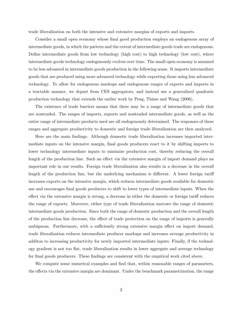
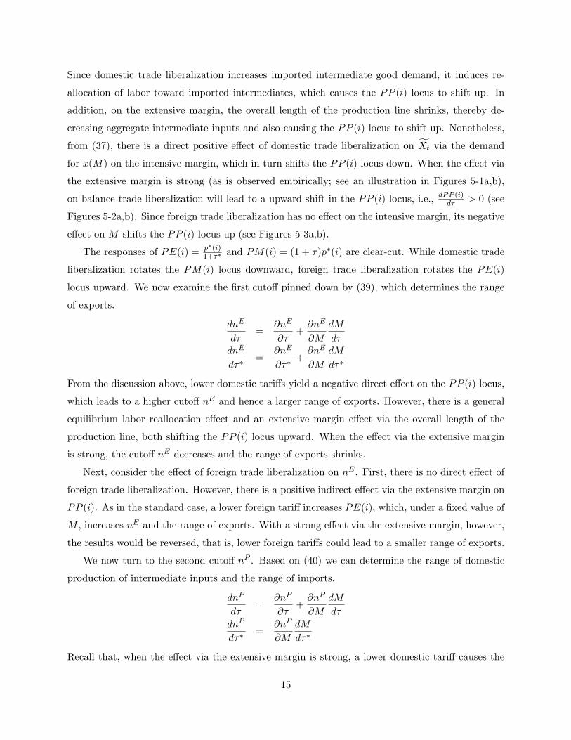
For now, assume that the home country produces all intermediate goods in the range�0; nPt
�and
they export intermediates in the range�0; nEt
�where nEt � nPt while intermediates in the range
5

�nPt ;Mt
�are imported (see Figure 1 for a graphical illustration). We will later verify this assertion
and solve for nEt , npt , and Mt endogenously.
The �rm that produces the �nal good has the following �rst-order condition with respect to
intermediate goods demand xt(i) given by,
dYtdxt(i)
= �� (� � )xt(i)�
24MtZ0
xt(i0)di
0
35 = pt(i), 8 i 2 [0;Mt] (7)
or,
pt(i) =
8>>><>>>:PEt(i) � p�t (i)
1+�� , 8 i 2 [0; nEt ]
PPt(i) � �� �xt(i)� eX�it = �� (� � )xt(i)� eXt, 8 i 2 [nEt ; nPt ]
PMt(i) � (1 + �)p�t (i), 8 i 2 [nPt ;Mt]
(8)
where fXt � Z Mt
0xt(i
0)di
0, eX�i
t, �Ri0 6= i xt(i
0)di
0= fXt � x(i). One can think of fXt as a measure of
aggregate intermediate good usage. This implies the following Proposition.
Proposition 1: (Demand for Intermediate Goods) Within the nontraded range [nEt ; nPt ], the de-
mand for intermediate good is downward sloping. If intermediate goods are Pareto substitutes
( > 0), then the larger aggregate intermediate goods is (higher eXt), the less individual intermedi-ate good demand will be.
Using Leibniz�s rule, the �nal �rm�s �rst-order condition with respect to the length of the
production line (Mt) can be derived as:4
dYtdMt
=
��� � �
2xt(Mt)� fXt�xt(Mt) = w�+ pt(Mt)xt(Mt) (9)
Manipulating these expressions yields the relative inverse demands for intermediate goods and the
demand for the M th intermediate good:
pt(i)� pt(i0) =
8>>><>>>:1
1+�� [p�t (i)� p�t (i
0)], 8 i; i0 2 [0; nEt ]
�(� � )[xt(i)� xt(i0)], 8 i; i0 2 [nEt ; nPt ]
(1 + �)[p�t (i)� p�t (i0)], 8 i; i0 2 [nPt ;Mt]
(10)
From (9), we have:
� � 2
[xt(Mt)]2 � [�� fXt � (1 + �)p�t (Mt)]xt(Mt) + w� = 0 (11)
Given � > , the solution to relative demand exists if [�� fXt � (1 + �)p�t (Mt)]2 > 2(� � )w�.
4 It is assumed there is a very large M� being produced in the world so that any local demand for M can be met
with imports from the rest of the world.
6

Proposition 2: (Relative Demand for Intermediate Goods) Within the nontraded range [nEt ; nPt ],
the relative demand for intermediate goods is downward sloping. Additionally, the stronger the
production sophistication e¤ect is (higher � � ), the less elastic the relative demand will be.Next, we determine how the intermediate goods sector works.
3.2 The Intermediate Sector
With local monopoly power, each intermediate �rm can jointly determine the quantity of interme-
diate good to supply and the associated price. By utilizing (3) and (4), its optimization problem is
described by the following Bellman equation:
V (At(i))8 i2[nEt ;nPt ]
= maxpt(i); yt(i); Lt(i); Ht(i)
[(pt(i)� �)yt(i)]� wt [Lt(i) +Ht(i)] +1
1 + �V (At+1(i)) (12)
s.t. (5), (6) and (8)
Before solving the intermediate �rm�s optimization problem, it is convenient to derive marginal
revenue:
d[(pt(i)� �)yt(i)]dyt(i)
= pt(i)� � + yt(i)dpt(i)
dyt(i)
= pt(i)� � � �yt(i)
= pt(i)� � � �At(i)Lt(i)� (13)
where pt(i) can be substituted out with (8).
Now we solve for the value functions for both nontraded intermediate goods i 2 [nEt ; nPt ] andexported intermediate goods i 2 [0; nEt ]. The �rst-order conditions with respect to the two labordemand variables is,
[pt(i)� � � �At(i)Lt(i)�]�At(i)Lt(i)��1 = wt 8 i 2 [nEt ; nPt ] (14)
�
1 + �VAt+1(i) t(i)Ht(i)
��1 = wt 8 i 2 [nEt ; nPt ] (15)
The Benveniste-Scheinkman condition with respect to the state variable At(i) is given by,
VAt = [pt(i)� � � �At(i)Lt(i)�]Lt(i)� +1� �1 + �
At+1(i) 8 i 2 [nEt ; nPt ] (16)
Similarly, we have the value function for i 2 [0; nEt ], as
V (At(i))8 i2[0;nEt ]
= maxpt(i); yt(i); Lt(i); Ht(i)
�[p�t (i)
1 + ��� �]At(i)Lt(i)� � wt [Lt(i) +Ht(i)]
+1
1 + �Vt+1[(1� �)At(i) + t(i)Ht(i)�]
�(17)
7

where we have used (6) and (8) for i 2 [0; nEt ]. We can obtain the �rst-order conditions with respectto Lt(i) and Ht(i), respectively, as follows:
�[p�t (i)
1 + ��� �]At(i)Lt(i)��1 = wt, 8 i 2 [0; nEt ] (18)
�
1 + �VAt+1(i) t(i)Ht(i)
��1 = wt, 8 i 2 [0; nEt ] (19)
The Benveniste-Scheinkman condition with respect to the state variable At(i) is given by,
VAt = [p�t (i)
1 + ��� �]Lt(i) +
1� �1 + �
VAt+1(i) = 0, 8 i 2 [0; nEt ] (20)
We now turn to solving the system for a steady state.
4 Steady-State Equilibrium
Since our focus is on e¢ cient production of the �nal good using a basket of intermediate goods,
we ignore households� intertemporal consumption-saving decision and labor-market equilibrium.
Thus, both the rental rate and the wage rate are exogenously given in our model economy. These
assumptions simplify our analysis of labor allocation and technology choice.
4.1 Labor Allocation
In steady-state equilibrium, all endogenous variables are constant over time. Thus, (6) implies:
H (i) =
��A (i)
(i)
� 1�
, i 2 [0; nP ] (21)
We can also rewrite (19) as:
VA =(1 + �)wH(i)1��
� (i), i 2 [0; nP ]
which can then be plugged into (20) to obtain:
(�+ �)wH(i)1��
� (i)
��A (i)
(i)
� 1���
= [p�(i)
1 + ��� �]L (i)� , 8 i 2 [0; nE ]
Using (18) and (21) to simplify the above expression, we have:
A (i) = A (i)L (i)� , 8 i 2 [0; nP ] (22)
where
A � 1
�1��
��
�(�+ �)
��> 0:
8

One can think of A as the technology scaling factor and (i) as the technology gradient that
measures how quickly technology improves as i increases.
Next, we substitute (8) and (22) into (18) to eliminate p (i) and A (i), yielding the following
expression in L(i) alone:
�[p�(i)
1 + ��� �]A (i)LE(i)�+��1 = w, 8 i 2 [0; nE ] (23)
which can be used to derive labor demand for i 2 [0; nE ]: LE(i) = f �w [p�(i)1+�� � �]A (i)g
11���� .
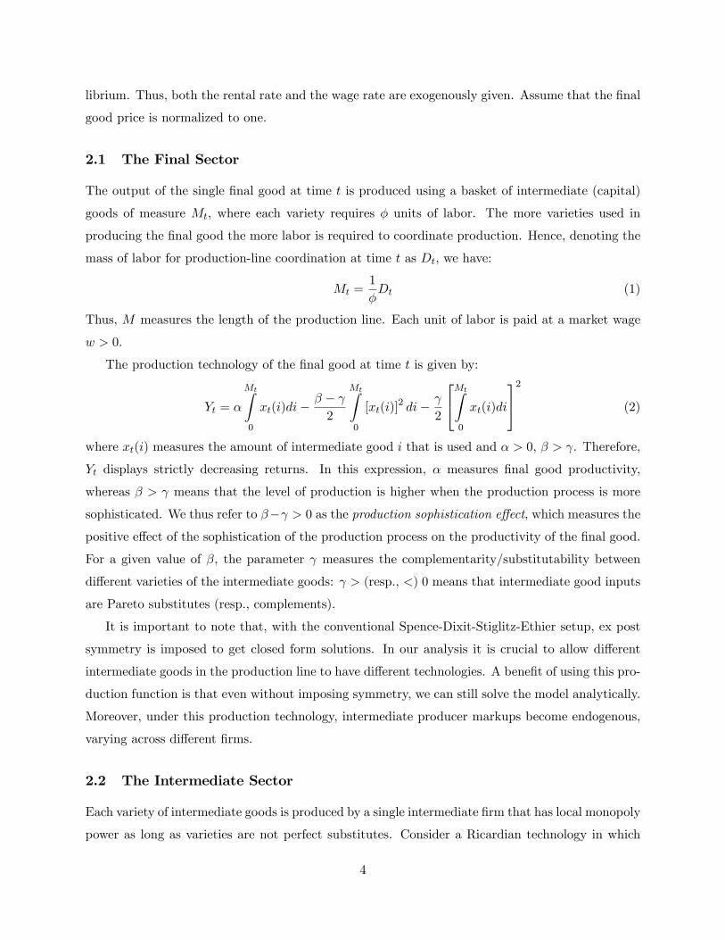
MPL(i)8 i2[nE ;nP ]
= �A (i)LP (i)�(1����) [�� � � eX�i � 2�A (i)LP (i)�+�] = w (24)
It is clear thatMPL(i) is strictly decreasing in L (i) with limL(i)�!0MPL(i) �!1 and limL(i)�!Lmax
MPL(i) = 0, where
Lmax �"�� � � eX�i
2�A (i)
# 1�+�
Figure 2 depicts the MPL(i) locus, which intersects w to pin down labor demand in steady-state
equilibrium (point E). It follows that dL(i)dw < 0 and dL(i)d� > 0, dL(i)d� < 0, dL(i)d� < 0 and dL(i)
d < 0.
That is, an increase in the �nal good productivity (�), or a decrease in the unit capital require-
ment (�), the magnitude of variety bias (�), or the degree of substitutability between intermediate
good varieties ( ) increases the intermediate �rm�s demand for labor. Note that the direct e¤ect of
improved e¢ ciency of investment in intermediate good production technology ( (i)) is to increase
the marginal product of labor and induce higher labor demand by intermediate �rms. This we call
the induced demand e¤ect. However, there is also a labor saving e¤ect. Under variable monopoly
markups, a better technology enables the intermediate �rm to supply less and extract a higher
markup which will save labor inputs. Thus, the overall e¤ect is generally ambiguous. Finally,
and also most interestingly, when �nal good production becomes more sophisticated (larger M),
it is clear that the eX�i will rise, thereby shifting the MPL(i) locus downward and lowering each
variety�s labor demand for a given wage rate. Summarizing these results we have:
Proposition 3: (Labor Demand for Intermediate Goods Production) Within the nontraded range
[nE ; nP ], labor demand is downward sloping. Moreover, an increase in �nal good productivity (�)
or a decrease in the overall length of the �nal good production line (M), the unit capital requirement
( �), the magnitude of variety bias (�), or the degree of substitutability between intermediate good
varieties ( ) increases the intermediate �rm�s demand for labor in the steady state.
Next, we can use (4), (21) and (23) to derive R&D labor demand and total labor demand by
9

each intermediate �rm as follows:
H(i) =��A� 1� L(i), 8 i 2 [0; nE ] (25)
N(i) = L(i) +H(i) =h1 +
��A� 1�
iL(i), 8 i 2 [0; nE ] (26)
Combining the supply of and the demand for the M th intermediate good, (5) with i = nP and (6),
we have
y(i) = A (i)L (i)�+� , i 2 [0; nP ] (27)
In equilibrium, we can re-write the supply of intermediate good i as:
y(i) =
8>>><>>>:x(i) + z�(i) > x(i),
x(i),
x(i) = z(i) > 0
if
i 2 [0; nE ]
i 2 [nE ; nP ]
i 2 [nP ;M ]
(28)
where z�(i) is home country exports of intermediate good i and z(i) is home country imports of
intermediate good i. Substituting (27) into (8), we have:
z�(i) = y(i)� x(i)
= A (i)L (i)�+� ��� eX � p�(i)
1+��
� � , 8i 2 [0; nE ] (29)
From (8) and (23), we can derive aggregate intermediate good usage as:
eX =
nPZ0
A (i)L (i)�+� di+
MZnP
z(i)di�nEZ0
z�(i)di (30)
The aggregate labor demand is given by,
N = �M +h1 +
��A� 1�
i264nPZ0
L(i)di
375 (31)
We assume that labor supply in the economy is su¢ ciently large to ensure the demand is met.
4.2 Technology Choice and Pattern of Production and Trade
The local country�s technology choice with regards to intermediate goods production depends cru-
cially on whether local production of a particular variety is cheaper than importing it. For con-
venience, we arrange the varieties of intermediate goods from the lowest technology to highest
technology. Without loss of generality, it is assumed that
(i) = (1 + � � i); �(i) = �(1 + �� � i) (32)
10

where 0 � �0 and � < ��.
From (7) and (8), we have:
x (i) =
8>>><>>>:xE(i) � �� eX� p�(i)
1+����
xP (i) � A (i)L (i)�+�
xM(i) � �� eX�(1+�)p�(i)��
if
i 2 [0; nE ]
i 2 [nE ; nP ]
i 2 [nP ;M ]
(33)
where L(i), i 2 [nE ; nP ], is pinned down by (23). Thus, the value of net exports of intermediategoods is:
E =1
1 + ��
nEZ0
p�(i)xE(i)di� (1 + �)MZnP
p�(i)xM(i)di (34)
Trade balance therefore implies that domestic �nal good consumption is given by,
C = Y + E (35)
That is, when the intermediate goods sector runs a trade surplus, the �nal good sector will have a
trade de�cit.
Notice that p(i) is decreasing in (i), which implies that better technology corresponds to lower
costs and hence lower intermediate good prices. As a result, it is expected that dp(i)di < 0; that is,
the intermediate good price function is downward-sloping in ordered varieties (i). Thus, we have
the following proposition.
Proposition 4: (Producer Price Schedule) Within the nontraded range [nE ; nP ], the steady-state
intermediate good price schedule is downward sloping in ordered varieties ( i).
This can then used to compute aggregate intermediate goods:
eX =
nPZ0
A (i)L (i)�+� di+
MZnP
z(i)di�nEZ0
z�(i)di
=
nPZ0
A (i)L (i)�+� di+
MZnP
�� eX � (1 + �)p�(i)� � di
�nEZ0
"A (i)L (i)�+� �
�� eX � p�(i)1+��
� �
#di
= A
nPZnE
(i)L (i)�+� di� 1
� �
264(1 + �) MZnP
p�(i)di+1
1 + ��
nEZ0
p�(i)di
375+�� eX� � (M + nE � nP )
11

or,
eX =
A
Z nP
nE (i)L (i)�+� di+ �
�� (M + nE � nP )� 1��
"(1 + �)
Z M
nPp�(i)di+ 1
1+��
Z nE
0p�(i)di
#1 +
�� (M + nE � nP )(36)
which we call the intermediate-good aggregation (XX) locus. In addition, by substituting (33) into
(11), we can get the boundary condition at M :
�� eX � (1 + �)p�(M) =p2(� � )w� (37)
which will be referred to as the production-line trade-o¤ (MM) locus.
Before characterizing the relationship between M and eX, it is important to check the second-order condition with respect to the length of the production line. From (11), and (36), we can
derive the second-order condition as:
Mx(M)
(1 + �)p�(M)> � M
p�(M)
dp�(M)
dM
Under the following world price speci�cation:
p�(i) = p� b � i
the second-order condition becomes:
Condition S: b < 1+�
q2w��� .
Thus, it is necessary to assume that intermediate goods are Pareto substitutes in producing the
�nal good ( > 0), which we shall impose throughout the remainder of the paper.
The next condition to check is the nonnegative pro�t condition for the intermediate-good �rms.
For i 2 [nE ; nP ], we have:
�(i) = [�� eX�i � � � �x(i)]A (i)L (i)�+� � wL(i)[1 + (�A)1� ] = �(i)wN(i) (38)
where the markup is de�ned as �(i) � p(i)���[1+(�A)1=�][p(i)����x(i)] � 1. For i 2 [0; n
E ], we have:
�(i) = [p�(i)
1 + ��� �]A (i)L (i)�+� � wL(i)[1 + (�A)
1� ]
= A (i)L (i)�+� [p�(i)
1 + ��� �]f1� �[1 + (�A)
1� ]g
Therefore, to ensure nonnegative pro�t, we must impose p(i)��p(i)����x(i) > �[1+(�A)
1� ] (i.e., �(i) > 0)
for i 2 [nE ; nP ] and �[1 + (�A)1� ] < 1 for i 2 [0; nE ]. Since the latter condition always implies the
former, we can simply specify the following condition to ensure positive pro�tability:
12

Condition N: �[1 + (�A)1� ] < 1.
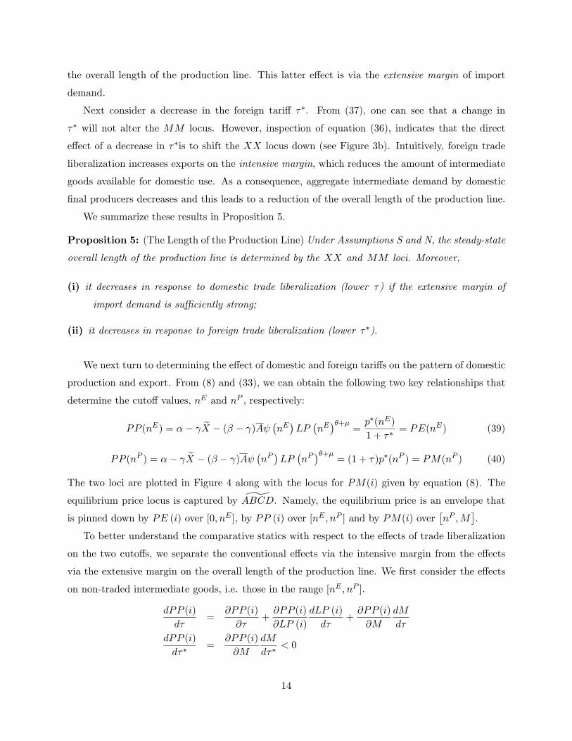
The MM and XX loci are drawn in Figure 3. The MM locus (equation (37)) and the XX
locus (equation (36)) are the loci that relate eX to M are both positively sloped. First, consider
the MM locus. Notice that since intermediate goods are Pareto substitutes, the direct e¤ect of an
increase in aggregate intermediate goods, eX, is to reduce the demand for each intermediate good.As M increases, the price of the intermediate good at the boundary, p�(M), falls, as does the cost
of using this intermediate good. This encourages the demand for x(M) and, to restore equilibrium
in (37), one must adjust eX upward, implying that the MM locus is upward sloping. The intuition
underlying the XX locus is more complicated. For illustrative purposes, let us focus on the direct
e¤ects. As indicated by (36), the direct e¤ect of a more sophisticated production line (higherM) is
to raise the productivity of manufacturing the �nal good as well as the cost of intermediate inputs.
While the productivity e¤ect increases aggregate demand for intermediate goods, the input cost
e¤ect reduces it. On balance, it is not surprising that the positive e¤ect dominates as long as such
an operation is pro�table. Nonetheless, due to the con�icting e¤ects, the positive response of eX to
M is not too large and, as a result, the XX locus is �atter than the MM locus. The equilibrium
is illustrated in Figure 3 by point E.
4.3 Trade Liberalization
4.3.1 E¤ects on Pattern of Production and Trade
We now consider the e¤ects of trade liberalization. We begin by determining the e¤ect of trade
liberalization on the overall length of the production line. Consider �rst a decrease in the domestic
tari¤ (�). This decrease in domestic protection lowers the domestic cost of imported intermediate
inputs i, (1 + �)p�(i) and hence increases demand. This causes the MM locus to shift up (see
Figure 3a). The e¤ect on the XX locus is, however, ambiguous. While there is a direct positive
e¤ect of domestic trade liberalization on eX, there are many indirect channels via the endogenouscuto¤s, nE and nP . While we will return to this later, our numerical results show that the shift of
the XX locus is small compared to the shift in the MM locus. Therefore, in this case one expects
the net e¤ect of domestic trade liberalization to decrease the overall length of the production line
(lower M) as seen in Figure 3a. This suggests that although domestic trade liberalization increases
imported intermediate inputs on the intensive margin, �nal producers react to it by shifting away
from imports of higher types to the cheaper lower type intermediate inputs, thereby decreasing
13
the overall length of the production line. This latter e¤ect is via the extensive margin of import
demand.
Next consider a decrease in the foreign tari¤ ��. From (37), one can see that a change in
�� will not alter the MM locus. However, inspection of equation (36), indicates that the direct
e¤ect of a decrease in ��is to shift the XX locus down (see Figure 3b). Intuitively, foreign trade
liberalization increases exports on the intensive margin, which reduces the amount of intermediate
goods available for domestic use. As a consequence, aggregate intermediate demand by domestic
�nal producers decreases and this leads to a reduction of the overall length of the production line.
We summarize these results in Proposition 5.
Proposition 5: (The Length of the Production Line) Under Assumptions S and N, the steady-state
overall length of the production line is determined by the XX and MM loci. Moreover,
(i) it decreases in response to domestic trade liberalization (lower �) if the extensive margin of
import demand is su¢ ciently strong;
(ii) it decreases in response to foreign trade liberalization (lower ��).
We next turn to determining the e¤ect of domestic and foreign tari¤s on the pattern of domestic
production and export. From (8) and (33), we can obtain the following two key relationships that
determine the cuto¤ values, nE and nP , respectively:
PP (nE) = �� eX � (� � )A �nE�LP
�nE��+�
=p�(nE)
1 + ��= PE(nE) (39)
PP (nP ) = �� eX � (� � )A �nP�LP
�nP��+�
= (1 + �)p�(nP ) = PM(nP ) (40)
The two loci are plotted in Figure 4 along with the locus for PM(i) given by equation (8). The
equilibrium price locus is captured by ABCD. Namely, the equilibrium price is an envelope that
is pinned down by PE (i) over [0; nE ], by PP (i) over [nE ; nP ] and by PM(i) over�nP ;M
�.
To better understand the comparative statics with respect to the e¤ects of trade liberalization
on the two cuto¤s, we separate the conventional e¤ects via the intensive margin from the e¤ects
via the extensive margin on the overall length of the production line. We �rst consider the e¤ects
on non-traded intermediate goods, i.e. those in the range [nE ; nP ].
dPP (i)
d�=
@PP (i)
@�+@PP (i)
@LP (i)
dLP (i)
d�+@PP (i)
@M
dM
d�
dPP (i)
d��=
@PP (i)
@M
dM
d��< 0
14
Since domestic trade liberalization increases imported intermediate good demand, it induces re-
allocation of labor toward imported intermediates, which causes the PP (i) locus to shift up. In
addition, on the extensive margin, the overall length of the production line shrinks, thereby de-
creasing aggregate intermediate inputs and also causing the PP (i) locus to shift up. Nonetheless,
from (37), there is a direct positive e¤ect of domestic trade liberalization on fXt via the demandfor x(M) on the intensive margin, which in turn shifts the PP (i) locus down. When the e¤ect via
the extensive margin is strong (as is observed empirically; see an illustration in Figures 5-1a,b),
on balance trade liberalization will lead to a upward shift in the PP (i) locus, i.e., dPP (i)d� > 0 (see
Figures 5-2a,b). Since foreign trade liberalization has no e¤ect on the intensive margin, its negative
e¤ect on M shifts the PP (i) locus up (see Figures 5-3a,b).
The responses of PE(i) = p�(i)1+�� and PM(i) = (1 + �)p�(i) are clear-cut. While domestic trade
liberalization rotates the PM(i) locus downward, foreign trade liberalization rotates the PE(i)
locus upward. We now examine the �rst cuto¤ pinned down by (39), which determines the range
of exports.
dnE
d�=
@nE
@�+@nE
@M
dM
d�dnE
d��=
@nE
@��+@nE
@M
dM
d��
From the discussion above, lower domestic tari¤s yield a negative direct e¤ect on the PP (i) locus,
which leads to a higher cuto¤ nE and hence a larger range of exports. However, there is a general
equilibrium labor reallocation e¤ect and an extensive margin e¤ect via the overall length of the
production line, both shifting the PP (i) locus upward. When the e¤ect via the extensive margin
is strong, the cuto¤ nE decreases and the range of exports shrinks.
Next, consider the e¤ect of foreign trade liberalization on nE . First, there is no direct e¤ect of
foreign trade liberalization. However, there is a positive indirect e¤ect via the extensive margin on
PP (i). As in the standard case, a lower foreign tari¤ increases PE(i), which, under a �xed value of
M , increases nE and the range of exports. With a strong e¤ect via the extensive margin, however,
the results would be reversed, that is, lower foreign tari¤s could lead to a smaller range of exports.
We now turn to the second cuto¤ nP . Based on (40) we can determine the range of domestic
production of intermediate inputs and the range of imports.
dnP
d�=
@nP
@�+@nP
@M
dM
d�dnP
d��=
@nP
@M
dM
d��
Recall that, when the e¤ect via the extensive margin is strong, a lower domestic tari¤ causes the
15

PP (i) locus to shift up. In addition, the PM(i) locus rotates downward. Both result in a lower
cuto¤ nP and hence a smaller range of domestic production. Should the overall length M be
unchanged, the range of imports would increase. But, since M shrinks, the net e¤ect on the range
of imports is generally ambiguous.
In response to a lower foreign tari¤, the only change is the upward shift in the PP (i) locus
via the shrinkage of M on the extensive margin. It is therefore, unambiguous to have a lower
cuto¤ nP and a smaller range of domestic production. This e¤ect is absent in the conventional
trade literature. To summarize, foreign trade liberalization does not a¤ect the range of domestic
imports. Again, since M shrinks, the range of imports need not increase.
We illustrate these comparative statics in Figures 5-1a,b and 5-2a,b and summarize the results
in Proposition 6.
Proposition 6: (The Range of Exports, Domestic Production and Imports) Under Assumptions S
and N, the steady-state pattern of international trade features exporting over the range�0; nE
�and
importing over the range�nP ;M
�where the range
�nE ; nP
�is nontraded. Moreover, the steady-
state equilibrium possesses the following properties:
(i) in response to domestic trade liberalization (lower �),
a. the import price PM(i) falls whereas the domestic producer price PP (i) increases if the
e¤ect via the extensive margin is strong;
b. both the range of exports�0; nE
�and the range of domestic production
�0; nP
�shrink if
the e¤ect via the extensive margin is strong;
(ii) in response to foreign trade liberalization (lower ��),
a. while the export price PE(i) always increases, the domestic producer price PP (i) also
increases if the e¤ect via the extensive margin is strong;
b. while the range of domestic production�0; nP
�always shrinks, the range of exports
�0; nE
�shrinks if the e¤ect via the extensive margin is strong;
(iii) in response to either domestic or foreign trade liberalization, the range of imports is generally
ambiguous.
16

4.3.2 Markups, Productivity and Technology
We next turn to consideration of the e¤ect of trade liberalization on markups. In the domestic
exporting range�0; nE
�, an intermediate �rm�s markup becomes trivial, depending positively on
foreign tari¤. That is, foreign trade liberalization will reduce domestic markups. In the nontraded
range i 2 [nE ; nP ], we can see from (38) that markups will respond endogenously to trade policy. Asshown in Proposition 6, in response to a reduction in the domestic tari¤ � , the domestic producer
price PP (i) rises when the e¤ect via the extensive margin is strong. Moreover, there is a shift
from domestic to imported intermediate inputs and hence x(i) falls. Both lead to lower markups
received by domestic intermediate good �rms. Thus, we have:
Proposition 7: (Markups) Under Assumptions S and N, domestic intermediate �rms�markups
in the steady-state equilibrium always decrease in response to foreign trade liberalization (lower ��)
and fall in response to domestic trade liberalization (lower �) if the e¤ect via the extensive margin
is strong.
We turn to determining how trade liberalization a¤ects productivity and technology. It can be
seen from Proposition 6 that under domestic trade liberalization, the range of domestic production�0; nP
�shrinks if the e¤ect via the extensive margin is strong. Thus, some higher technology
intermediate goods are now imported, which are produced in the North with lower costs, thereby
resulting in unambiguous productivity gains. The e¤ect on average productivity is, however, not
obvious. De�ne the aggregate technology used by domestic producers as eA =
Z nP
0A (i;M) di.
Utilizing (22), we can write:
eA = A
nPZ0
(i)LP (i)� di (41)
Consider the benchmark case where the extensive margin of import demand is su¢ ciently strong.
Then, domestic trade liberalization (lower �) will reduce the overall length of the production line
as well as the range of domestic production. While the latter decreases aggregate technology, the
former raises individual labor demand and hence individual technology used for each intermediate
good employed by the domestic �nal producer (recall Proposition 3). Thus, to domestic producers,
when the extensive margin of import demand is strong, domestic trade liberalization can reduce
average technologyeAnPas long as the technology gradient (i) is not too �at. Nonetheless, average
productivity measured by YeX will increase due to the use of more advanced imported intermediate
inputs with a su¢ ciently strong extensive margin. Applying Proposition 6, we can see that foreign
17

trade liberalization will lead to a similar outcome in average technology and average productivity.
These results can be summarized in the following proposition.
Proposition 8: (Productivity) Under Assumptions S and N with a su¢ ciently strong extensive
margin of import demand, domestic trade liberalization results in productivity gains for newly im-
ported intermediate goods as well as an increase in average productivity. Moreover, foreign trade
liberalization also leads to higher average productivity. If, in addition, the technology gradient is
not too �at, both aggregate and average technology by domestic producers are lower in response to
domestic or foreign trade liberalization (lower � or ��).
This result is interesting because it points out that productivity and technology do not always
move together. In this model, trade liberalization leads to higher productivity because input prices
fall. This fall in input prices leads to a lower level of technology being chosen in equilibrium as
lower productivity inputs are used more intensively while the range of intermediate goods used
decreases. This latter e¤ect means that a lower level of technology is used by producers.
5 Numerical Analysis
Since some of the theoretical results are ambiguous we present some numerical examples to illustrate
how trade liberalization might work. For our baseline economy we set the time preference rate as
� = 7:5% and the technology obsolescence rate as � = 25%. We select the intermediate sector
production parameters as � = 0:5 and � = 0:2, which satis�es the requirement for decreasing
returns to scale, � + � < 1. We choose the �nal sector production parameters as � = 10, � = 0:2
and = 0:1, satisfying the requirements, � � > 0. Normalize � = 1 and set � = 0:05. The
technology and world price schedules are given by: (i) = 5 (1 + 0:1 � i) and p�(i) = 2:5 � 0:05 � i.Letting w = 50, this insures that both Conditions S and N are satis�ed. Finally, we choose
� = 7:5% > �� = 5%.
The computed ranges of exports, nontraded intermediate goods and imports turn out to be:
[0; nE ] = [0; 9:04], [nE ; nP ] = [9:04; 12:05] and [np;M ] = [12:05; 21:62], respectively. The average
markup of domestic non-exporting producers is:~�
nP�nE �
Z nP
nE
�(i)di
nP�nE = 0:768. While aggregate
intermediate goods turns out to be eX = 77:68, aggregate and average technology used by domes-
tic producers are eA = 963:94 andeAnP
= 80:00, respectively. The computed �nal good output is
Y = 301:84 and the corresponding productivity measure is YeX = 3:89. By including the domestic
tari¤ revenue R = �
Z M
nPp�(i)x(i)di, the augmented productivity measure becomes Y+ReX = 3:99.
18

Moreover, total values of intermediate goods exports and imports are 172:47 and 120:65, respec-
tively, and net exports are 51:81, implying that the �nal good is imported import for balanced
trade. Per capita �nal good consumption turns out to be 0:0311. In this benchmark economy, the
extensive margin of import demand is su¢ ciently strong for the overall length of the production
line to play a dominant role.
Now consider domestic trade liberalization in the form of a one percentage point decrease in the
domestic tari¤ which lowers � to 6:5%. The overall length of the production line M shrinks from
21:62 to 20:66. Again, with strong e¤ects viaM on the extensive margin, both the range of exports
and the range of domestic production decrease. In particular, the computed range of exports falls
to [0; nE ] = [0; 7:78]. The range of nontraded intermediate goods is [nE ; nP ] = [7:78; 10:95] which
means the range increases from 3:01 to 3:17, however, the overall range of home produced goods
shrinks. The range of imports is now [np;M ] = [10:95; 20:66] which is a slightly increased range. So
trade liberalization increases the range of non-traded and imported goods, but the range of exports
decreases by a large amount leading to a smaller range of intermediate goods used to produce
the �nal good. Aggregate intermediate goods usage falls slightly to eX = 77:31 indicating that the
increase in the intensive margin does not quite compensate for the decrease in the extensive margin.
Since in our benchmark economy, the technology gradient is not too �at, aggregate and average
technology used by domestic producers actually fall to eA = 782:35 and eAnP= 71:47. Moreover, the
average markup of domestic non-exporting producers decreases sharply to~�
nP�nE = 0:711. What
happens to output and productivity? Both of them increase signi�cantly. Computed �nal good
output increases to Y = 357:53 and productivity increases to YeX = 4:62. Including the domestic
tari¤ revenue, augmented productivity measure increases to Y+ReX = 4:72. Exports decrease to
148:94 while imports increase slightly to 125:09, thereby causing intermediate goods net export to
fall to 23:85. In this case, per consumption rises sharply to 0:0444.
Next, starting from our benchmark equilibrium, consider foreign trade liberalization, in the
form of a one percentage point decrease in the foreign tari¤ to �� = 4%. The overall length of the
production line M shrinks from 21:62 to 19:84. Again, with strong e¤ects via M on the extensive
margin, both the range of exports and the range of domestic production decrease. Moreover, the
range of imports is also narrowed slightly. In aggregate quantities, both total exports and total
imports drop whereas net export of intermediate goods shrinks sharply from 51:81 to 5:63. As
a result of the reduced length of the production line, aggregate intermediate goods fall, but, not
surprisingly, the reduced tari¤ distortion causes �nal good output to increase to Y = 397:50 and
measured productivity to rise sharply to YeX = 5:18. Moreover, the average markup of domestic non-
19

exporting producers falls to 0:681, the average technology used by domestic producers decreases to
62:80, whereas per capita consumption increases to 0:0603.
We have done several other numerical exercises but will only report one additional experiment.
Speci�cally, we consider an environment with global trade liberalization such as WTO or bilat-
eral/multilateral trade agreements, say, with both domestic and foreign tari¤ falling by 10%. In
this case, both the �nal good output and the measured productivity rise sharply, from Y = 301:84
and YeX = 3:89, to Y = 391:11 and YeX = 5:09, respectively, despite a reduction in average technology
used by domestic producers and average markup of domestic non-exporting producers. Notably, a
moderate 10% reduction in trade costs globally can lead to large production and e¢ ciency gains
where both aggregate output and average productivity rise by about 30%.
6 Concluding Remarks
We have constructed a dynamic model of intermediate goods trade to determine both the pattern
and the extent of intermediate goods trade. We have established that, although domestic trade
liberalization increases imported intermediate inputs on the intensive margin, �nal goods producers
react to it by shifting imports to lower types of intermediate inputs to lower the production cost.
This decreases the overall length of the production line.
When such an e¤ect via the extensive margin is strong, both domestic and foreign trade lib-
eralization lead to a reduction of the ranges of export and domestic production, but their e¤ects
on the range of imports are generally ambiguous. We have shown that, when the extensive margin
e¤ect of import demand is su¢ ciently strong, domestic trade liberalization leads to lower markups
and greater competition and results in productivity gains. If, in addition, the technology gradi-
ent is not too �at, then such productivity gains from trade liberalization can be associated with
lower aggregate and average technology by domestic intermediate goods producers. We have also
established numerically that trade liberalization (lower domestic and foreign tari¤s) can yield large
bene�ts to �nal goods producers, resulting in sharp increases in both the �nal good output and
measured productivity.
20

References
[1] Amiti, Mary and Jozef Konings (2007), �Trade Liberalization, Intermediate Inputs, and Pro-
ductivity: Evidence from Indonesia,�American Economic Review 97, 1611-1638.
[2] Ethier, Wilfred (1982), �National and International Returns to Scale in the Modern Theory
of International Trade,�American Economic Review 73, 389-405.
[3] Dornbusch, Rudiger (1992), �The Case for Trade Liberalization in Developing Countries,�
Journal of Economic Perspectives 6, 69-85.
[4] Edwards, Sebastian (1993), �Trade Liberalization, and Growth in Developing Countries,�Jour-
nal of Economic Literature 31, 1358-1393.
[5] Fernandes, Ana M. (2007), �Trade Policy, Trade Volumes and Plant-Level Productivity in
Colombian Manufacturing Industries,�Journal of International Economics 71, 52-71.
[6] Ferreira, Pedro Cavalcanti, and José Luiz Rossi (2003), �New Evidence from Brazil on Trade
Liberalization and Productivity Growth,�International Economic Review 44, 1383-1405.
[7] Flam, Harry and Elhanan Helpman (1987), �Vertical Product Di¤erentiation and North-South
Trade,�American Economic Review 77, 810-822.
[8] Goldberg, Pinelopi, Amit Khandelwal, Nina Pavcnik, and Petia Topalova (2011), �Imported
Intermediate Inputs and Domestic Product Growth: Evidence from India,�Quarterly Journal
of Economics, forthcoming.
[9] Hummels, David, Jun Ishii, and Kei-Mu Yi (2001), �The Nature and Growth of Vertical
Specialization in World Trade,�Journal of International Economics 54, 75�96.
[10] Keller, Wolfgang (2000), �Do Trade Patterns and Technology Flows A¤ect Productivity
Growth?�World Bank Economic Review 14, 17-47.
[11] Khandelwal Amit and Petia Topalova (2011), �Trade Liberalization and Firm Productivity:
The Case of India,�Review of Economics and Statistics 93, 995-1009.
[12] Kim Euysung (2000), �Trade Liberalization and Productivity Growth in Korean Manufactur-
ing Industries: Price Protection, Market Power, and Scale E¢ ciency,�Journal of Development
Economics 62, 55-83.
[13] Pavcnik, Nina (2002), �Trade Liberalization, Exit, and Productivity Improvements: Evidence
from Chilean Plants,�Review of Economic Studies 69, 245-276.
21

[14] Peng, Shin-Kun, Jacques-F. Thisse and Ping Wang (2006), �Economic Integration and Ag-
glomeration in a Middle Product Economy,�Journal of Economic Theory 131, 1-25.
[15] Yi, Kei-Mu (2003), �Can Vertical Specialization Explain the Growth of World Trade?�Journal
of Political Economy 111, 52-102.
22
Figure 1. Determination of Intermediate Goods Allocation
produced import
︷︷produced import
Etn P
tn tMexport

Figure 2. Labor Allocation
MPL(i)
M↓, τ↓, τ*↓
( )
ww
E E'
)( )(iLL

Figure 3. Determination of Length of Production Line
( )(a) X~
E XX
MM
''E
'E
↓
MM'M ''M
(b)
XX
MM
E
X~
*
E
'E ↓
M'M M

Figure 4. Technology Choice and Trade in Intermediate Goods
)(),( * ipip
p)1(
p
)(iPM
A
B
*1 p
)(iPE
)(iPP
)(ip
C
D
0 iMexport
d
Pnb
pEn
D
produceimport

Figure 5. Determination of Technology and Trade Pattern
1 ( ) 1 (b)PP(i),PE(i)
PP(i) PM(i)1-(a) 1-(b)
E
'E
PP(i),PE(i)
E
'E
)(iPM
PP(i),PM(i)
iiEn
)( iPP
)(iPE
)(iPP
E
Pn
tt XM~
EniPP )(◎ Direct effect :
◎ Indirect effect :
)(,)(~ PP
t nPPniPPXM
PE nn MPL (i)↑ PP (i)↓
2-(b)2-(a) PP(i),PE(i)
'E
)(iPE
PP(i),PM(i)
'E
)(iPM
i
E
)(iPP
i
E
)(iPP
( ) , PPM i n↓ ↓◎ Direct effect :
◎ Indirect effect :
)(iPE
◎
◎ no change
( ) ( )X MPL i PP i ↓ ↓ ↑ ( )X PP i ↓ ↑
τ↓ τ↓
iEn Pn

3-(a) 3-(b) PP(i),PE(i)
PP(i),PM(i)
)(iPM
E
E
'E
)(iPP
)(iPE
i i
E
)(iPP
pP
'E
* ↓Direct effect :
( if the direct effect is dominant )
* ↓PP (i) ↑, PM (i) no change, ↓
PE (i) ↑,PP (i) ↑ En ↓
Enb
pPn
Pn
Top Related