


Languages
Pages
Legal


Innovation and Product Reallocation in the Great Recession
David Argente
University of Chicago
Munseob Lee
University of Chicago
Sara Moreira
Northwestern University
April 2017[Link to the latest version]
Abstract
We exploit detailed product- and firm-level data to study the sources of innovation andthe patterns of productivity growth in the consumer goods sector over the period 2007-2013.Using a dataset that contains information on the product portfolio of each firm, we documentseveral new facts on product reallocation, a concept closely tied to several theories of growth.First, we calculate that every quarter around 8 percent of products are reallocated in theeconomy, and entry and exit of products is prevalent among di↵erent types of firms. Second,we find that most reallocation of products occurs within the boundaries of the firm. Entryand exit of firms have only a small contribution in the overall creation and destruction ofproducts. Third, we document that product reallocation is strongly procyclical and declinedby more than 30 percent during the Great Recession. This cyclical pattern is almost entirelyexplained by a decline in within firm reallocation. Motivated by these facts, we study thecauses and consequences of reallocation within incumbent surviving firms. As predicted bySchumpeterian growth theories, the rate of product reallocation strongly depends on theinnovation e↵orts of the firms and has important implications for revenue growth, productquality improvements, and productivity dynamics. Our estimates suggest that the declinein product reallocation through these margins contributed importantly to the slow growthexperienced after the Great Recession.
JEL Classification Numbers: E3, O3, O4.
Keywords: Innovation, Reallocation, Productivity, Great Recession
This paper is currently in preparation for the Carnegie-Rochester-NYU Conference Series on Public Policy.Email: [email protected]. Address: 1126 E. 59th Street, Chicago, IL 60637.Email: [email protected]. Address: 1126 E. 59th Street, Chicago, IL 60637.Email: [email protected]. Address: 2211 Campus Drive, Evanston, IL 60208.

1 Introduction
For decades, economists have identified product entry and exit as the key mechanism through
which product innovation translates into economic growth (Aghion and Howitt, 1992; Grossman
and Helpman, 1991; Aghion, Akcigit and Howitt, 2014). But despite the important theoretical
implications of product innovation, little is known empirically about the processes of creation and
destruction of products, and how these processes di↵er across di↵erent types of firms. In this paper
we study product reallocation across and within producers and how it evolved during the Great
Recession. What is the role of product reallocation on output growth and quality improvements
in the recent decade? How sensitive is innovation by new firms, small incumbents, and large
incumbents to changes in aggregate economic conditions? New evidence on these questions will
help understand how resources are allocated to their best use within an economy and inform the
recent debate on the sources of productivity slowdown in the U.S. (Davis and Haltiwanger, 2014;
Decker, Haltiwanger, Jarmin and Miranda, 2014).
We begin by assessing the magnitude of product creation and destruction in the consumer
goods sector over the period 2007Q1–2013Q4. We exploit detailed product- and firm-level data
at the barcode level to find that new products are systematically displacing existing products
in the market. Every quarter more than 10 percent of products are reallocated in the economy
with almost equal contribution of product entering and exiting the market. This is particularly
relevant for large and well-diversified firms, those that sell products in several product categories.
Consistent with several theories of creative destruction, we find that firms expanding, as well as
firms contracting, contribute to the overall destruction of products. This source of dynamism in
the U.S. economy occurs within the boundaries of the firm, and as a result of entry and exit of
new firms. We find that most product reallocation is made by surviving incumbent firm that add
or drop products in their portfolio.
After documenting that magnitude and pervasiveness of reallocation of products, we evaluate
the evolution during and post the great recession. We find that product reallocation is strongly
procyclical; the quarterly reallocation rate declined by more than 30 percent during the Great
Recession. To better understand the sources of the cyclicality in the reallocation rate we decompose
it in a within and a between firms component. We find that the cyclical pattern is overwhelmingly
a consequence of within firm reallocation. In particular, most of the decline in reallocation within
firms resulted from the decline in the creation of products during the recession.
In the second part of the paper we provide evidence that the decline in dynamism in the product
market a↵ected economic growth and the recovery after the Great Recession. Schumpeterian
growth models have traditionally linked the speed of product reallocation to the innovation e↵orts
of the firms and to subsequent gains in productivity. To uncover the causes and consequences
of the reallocation slowdown, we begin by establishing that the speed of product reallocation is
strongly related to the innovation e↵orts of the firms as captured by their expenditures on research
1

and development. This is consistent with theories featuring creative destruction where new and
better varieties replace obsolete ones.
The paper then establishes the relationship between product reallocation, as measured in our
dataset, and several innovation outputs such as revenue growth, product quality improvements,
and productivity growth. To do so, we follow Akcigit and Kerr (2010) and distinguish between
two di↵erent types of innovation from the perspective of the firms: incremental innovations and
extensions. Incremental innovations, represent new products within the existent product lines of
the firms, where they can exploit their capabilities and resources and benefit from economies of
scale or scope. Extensions, represent products beyond the main lines of business of the firms.
They are less common than incremental innovations because they represent larger innovations,
which are likely to be more costly to develop in the first place. We document that incremental
innovations have an immediate large impact on revenue. Extensions, on the other hand, are
in general more innovative new products launched with higher average quality and have higher
impact on the total factor productivity of the firm. In a similar way, we divide product exits in
two types: products that are more likely to be terminated due to creative destruction (replaced
by new products within the same product category) and those that were phased out due to the
scaling down firms’ operations (products without replacement). Consistent with Schumpeterian
theories1, exits due to creative destruction are correlated with gains in total factor productivity.
Overall, we find that firms that have higher reallocation rates grow faster, launch products with
higher average quality, and experience larger gains in productivity. Our evidence suggests that
the decline of reallocation experienced during the recession can explain around 15% of the drop in
aggregate productivity in this period and had substantial implications for economic growth in the
years that followed.
For most of our analysis, we rely primarily on the Nielsen Retail Measurement Services (RMS)
scanner dataset. It consists of more than 100 billion observations of weekly prices, quantities,
and store information of approximately 1.4 million products identified at the barcode level. We
combine information of prices with the weight and volume of the product to compute unit values
in order to approximate the quality of each product. In addition, we identify the firm owning
each UPC by obtaining information from GS1, the single o�cial source of barcodes in the United
States. The GS1 data contains the list of all U.S. barcodes along with information on the firms
that own them. Our combined dataset allows us to have revenue, price, quantity, and quality for
each product of a firm’s portfolio and allow us to study how the within and between margin of
product entry and exit evolve over time. Finally, we complement our dataset with Compustat to
obtain measures of total factor productivity and research and development expenses. To the best
of our knowledge, our paper is the first one to link the product level information available in the
Nielsen RMS with firm level observables available in other datasets.
Our paper contributes to several active research areas. Despite the vast theoretical implications
1See Aghion, Akcigit and Howitt (2014) for more details.
2

of product reallocation, the empirical analysis on the aggregate behavior of product reallocation
lags far behind its theoretical counterpart due to data limitations. The extant literature on real-
location has focused on the input markets using establishment and labor market data (Davis and
Haltiwanger, 1992; Foster, Haltiwanger and Krizan, 2001, 2006). By contrast, we focus on reallo-
cation in output markets. Importantly, our dataset allows us to study the relative contribution of
incumbents to the aggregate reallocation rate without inferring it from their job flows information.
Few papers have studied the degree of product reallocation directly. Bernard, Redding and
Schott (2010) study the extent of product switching within firms using production classification
codes (five-digit SIC codes). Given the level of aggregation of their data, in their work several
firms could produce the same product. We substantially improve on this by measuring products
at a much finer level using scanner data. This allows us to explore the dynamics of each firms’
unique portfolio of products as opposed to study the dynamics of their product lines. Our work is
also closely related to Broda and Weinstein (2010) who study the patterns of product entry and
exit using a similar dataset to ours but collected from consumers rather than stores. Collecting
data at the store level o↵ers the advantage of observing, for the categories available, the entire
universe of products for which a transaction is recorded in a given week rather than the products
consumed by a sample of households. Therefore, our dataset allows us to cover less frequently
consumed goods and provides less noisy measures of entry and exit of products. Our paper builds
on their work by examining between and within firm reallocation separately and examining the
contribution of each of these components during the Great Recession. Moreover, we examine the
reallocation patterns of firms subdividing them in several di↵erent dimensions: according to their
size, their level of diversification (i.e. firms selling in a single product category versus firms selling
in multiple product categories) and whether they are expanding or contracting at a given point in
time.
Furthermore, by studying the connection between reallocation and di↵erent measures of inno-
vation, our work links studies on reallocation, which focus mainly on moving resources from less to
more e�cient uses to enhance productivity growth, to the parallel literature on innovation (Klette
and Kortum, 2004; Lentz and Mortensen, 2008; Akcigit and Kerr, 2010; Acemoglu, Akcigit, Bloom
and Kerr, 2013; Garcia-Macia, Hsieh and Klenow, 2016). Although we examine only the retail
sector of the economy, to the best of our knowledge, our paper is the first to establish empirically
the relationship between product entry and exit and the innovation activities of the firms. In
particular, our matched dataset allows us to test and validate empirically several predictions of
Schumpeterian growth models; prediction that have been hard to examine in the past due to data
availability issues.
Lastly, our work is related to literature in firm dynamics that studies the propagation of ag-
gregate shocks after large contractions in output (Caballero and Hammour, 1994; Moreira, 2016).
We document that both the reallocation rate and the entry rate of products su↵ered a persistent
decline after the Great Recession. The decline of product creation had consequences in terms of
3
revenue for the firms in the short-run. But, more importantly, this missing generation of prod-
ucts, in the spirit of Gourio and Siemer (2014), combined with the evidence we provide on the
relationship between reallocation and productivity growth, have substantial implications for the
slow recovery experienced by the U.S economy in the years following the Great Recession.
The rest of the paper is organized as follows. Section 2 presents the data and describes our
procedure to link our product level dataset with firm level information available in Compustat.
In section 3, we define reallocation and provide several decompositions to explore the relative
contributions of the between and within margins. In this section we also provide an interpretation
of the magnitudes of the reallocation rate we observe and describe its evolution during the Great
Recession. In section 5 we examine the possible determinants of rellocation. We examine its
relationship with R&D and define incremental innovations and extensions along with exits due
to creative destruction and terminations due to firms scaling down their operations. Section 6
tests and validates the predictions of models involving creative destruction and documents the
relationship between reallocation and revenue growth, quality improvements, and productivity
dynamics. Section 7 concludes. We include several robustness tests and additional empirical
findings in the Appendix.
2 Data Description
2.1 Baseline Product-Level Dataset
We rely primarily on the Nielsen Retail Measurement Services (RMS) scanner dataset, which is
provided by the Kilts-Nielsen Data Center at the University of Chicago Booth School of Business.
The RMS consists of more than 100 billion unique observations at the week ⇥ store ⇥ UPC level.2
Each individual store reports weekly prices and quantities sold for every UPC code that had any
sales volume during the week.
The data is generated by point-of-sale systems and contains approximately 40,000 distinct stores
from 90 retail chains across 371 MSAs and 2,500 counties between January 2006 and December
2014. The data set includes around 12 billion transactions per year worth, on average, 220 billion.
Over our sample period the total sales across all retail establishments are worth approximately
2 trillion and represent 53% of all sales in grocery stores, 55% in drug stores, 32% in mass
merchandisers, 2% in convenience stores, and 1% in liquor stores.
The baseline data consist of approximately 1.64 million distinct products identified by a unique
UPC. The data is organized into 1,070 detailed product modules, aggregated into 114 product
groups, which are then grouped into 10 major departments.3 For example, a 7-ounce bag of Pringles
2A Universal Product Code (UPC) is a code consisting of 12 numerical digits that is uniquely assigned to eachspecific item.
3The ten major departments are: Health and Beauty aids (e.g. cosmetics, pain remedies), Dry Grocery (e.g.baby food, canned vegetables), Frozen Foods, Dairy (e.g. cheese, yogurt), Deli, Packaged Meat, Fresh Produce,
4
Select Potato Crisps, Bold Crunch Jalapeno Ranch has UPC 037000213758 is produced by Procter
& Gamble and it is mapped to product module ”Potato Chips” in product group ”Snacks”, which
belongs to the ”Dry Grocery” department.4 Each UPC contains information on the brand, size,
packaging, and a rich set of product features including the weight and the volume of the product
which we use to compute unit values.
Our data set combines all sales at the national and quarterly level; although we also conduct
some exercises at the annual frequency given that some firm level observables are only available at
that frequency. For each product j in quarter t, we define revenue r
jt
as total revenue across all
stores and weeks of the quarter. Likewise, quantity q
jt
is defined as total quantities sold across all
stores and weeks of the quarter. Price p
jt
is defined by the ratio of revenue to quantity, which is
equivalent to quantity weighted average price.
For each product we use the panel structure to measure the entry and exit periods.5 We follow
Broda and Weinstein (2010) and Argente and Yeh (2016) to use the UPC as the main product
identifier. This is because it is rare that a meaningful quality change occurs without resulting
in a UPC change. Two concerns may arise from this assumption. Chevalier, Kashyap and Rossi
(2003) notes that some UPCs might get discontinued only to have the same product appear with
a new UPC. This is not a concern in our data set because Nielsen detects these UPCs and assigns
them their prior UPC. The second concern is that companies could recycle UPCs and use them for
di↵erent products. Nielsen also identifies these UPCs and assigns them a di↵erent UPC version,
which we use to identify products.
We define entry as the first quarter of sales of a product and exit as the first quarter after we
last observe a product being sold.6 To study the entry- and exit rates patterns we use information
for all products in the period 2007Q1–2013Q4, that include cohorts born from 2007Q1 to 2013Q4
Non-Food Grocery (e.g. detergent, pet care), Alcohol and General Merchandise (e.g. batteries/flashlights, com-puter/electronic).
4In the product group ”Snacks” several product modules include: dips, potato chips, tortilla chips, meat, pretzels,popcorn, crackers, trail mix, and health bars.
5A critical part of our analysis is the identification of entries and exits. In comparison to other scanner datasetscollected at the store level, the RMS has a much wider coverage of products and stores. Table I shows that incomparison to the IRI Symphony dataset, a similar dataset widely used in the academic literature, the RMS coversmore 14 times the number of products in a given year. In terms of revenue the RMS represents roughly 2 percentof total household consumption whereas the IRI Symphony is 30 times smaller. In comparison to scanner datasetscollected at the household level, the RMS has also a wider coverage of products because it reflects the universeof transactions for the categories it covers as opposed to the purchases of a sample of households. The NielsenHomescan, for example, which contains information on the purchases of 40,000-60,000 U.S households covers lessthan 60% of the products the RMS covers in a given year.
6A product is first observed in the RMS dataset when a store sells it for the first time. Firms often do notintroduce goods in di↵erent stores at the same time, and thus, when we first observe a new UPC it may take sometime until it is disseminated across stores. Likewise, firms may stop producing a good in a certain time and wecan still see some transactions after that, as stores may still have some inventories. In the Appendix, we consideralternative definitions, where entry is defined as the second quarter of sales of a good, and exit as the second quarterto the last that we observe a product being sold. Relative to the definition of entry (exit) as the first (last) quarterwhere sales are registered, this last measure is more likely to represent a full quarter of sales, instead of just a fewweeks.
5
and cohorts born before that period, from whom we cannot determine the cohort and age.7 In
addition, given that our estimates of product entry and exit may be a↵ected by the entry and exit
of stores in the sample, we consider only a balanced sample of stores during our sample period.
Our final sample is described in Table III. Every year, on average more than 600,000 distinct
UPCs are present in our sample sold in a total of 33,056 stores. Most products have revenue of
less than 500 dollars per year but almost 5% of the products make more than 50 million dollars.
A product module contains approximately 582 products, a product group 5,459 products, and a
department 62,236 products on average. The table shows that these numbers remain very stable
before, during and after the Great Recession.
In order to minimize concerns of potential measurement error in the calculation of product
entry and exit, our baseline sample excludes private label products, considers products with at
least one transaction per quarter after entering, and excludes products in the Alcohol and General
Merchandise departments. We exclude private label goods because, in order to protect the identity
of the retailer, Nielsen alters the UPCs associated with private label goods. As a result, multiple
private label items are mapped to a single UPC making it di�cult to interpret the entry and
exit patterns of these items since it is not possible to determine the producer of these goods. We
consider products without missing quarters in order to rule out the possibility that our results are
driven by seasonal products, promotional items, or products with very small revenue. And, finally,
we exclude the two departments for which the coverage in our data is smaller and less likely to be
representative.
Nonetheless, all the results that follow are robust to using the full sample of products available
in the RMS. We present these results in Appendix D. Lastly, Appendix D also includes results
where, instead of using the barcode as the main product identifier, we identify products using
a broader definition using the product attributes provided by Nielsen as in Kaplan and Menzio
(2014). Under this alternative definition, a good is the same if it shares the same observable
features, the same size, and the same brand, but may have di↵erent UPCs. We use this definition
to minimize the concern that new products, when identified by their barcodes, represent only
marginal innovations from the perspective of the firms. Under this definition, each new entry
represents at least a new product line for the firm. Appendix D shows that the results we describe
below on the aggregate reallocation rate and on the impact of product reallocation on several
innovation outputs remain very similar under this specification.
7Note that we excluded the first four and last four quarters of the sample. Because we define entry as the firstquarter of sales of a product and exit as the first quarter after we last observe a product being sold, we may identifyan abnormally high entry in the first quarters and abnormally high exit in the last quarters. Our procedure ensuresthat we only classify as entrant a product that was not observed for at least for a full year before, and as exiter aproduct that we no longer observe for at least a full year past exit.
6

2.2 Matching Firm and Products
We link companies and products using information obtained from GS1 US, the single o�cial source
of barcodes. In order to obtain a barcode, companies must first obtain a GS1 Company Prefix. The
prefix is a 5-10 digits number that identifies companies and their products in over 100 countries
where GS1 is present. The number of digits in a Company Prefix indicates di↵erent capacities for
companies to create barcodes. For example, a 10 digits Company Prefix allows firms to create 10
unique barcodes and a 6 digits prefix allows them to create up to 100,000 unique items.8 Although
the majority of companies own a single prefix, it is not rare to find that some own several. Small
firms, for example, often obtain a larger prefix first, which is usually cheaper, before expanding
and requesting a shorter prefix.9 Larger firms, on the other hand, usually own several Company
Prefixes due to past mergers and acquisitions activities. For example, Procter & Gamble owns the
prefixes that used to belong to firms it acquired such as Old Spice, Folgers, and Gillete. Our GS1
data accounts for all mergers and acquisitions that occurred before October 2013. For consistency,
in what follows we perform the analysis at the parent company level.
Given that the GS1 US data contains the universe Company Prefixes generated in the US, we
combine these prefixes with those present in each UPC code in the RMS.10 Our combined data set
allows us to compute revenue, price, quantity, and quality for each product in a firm’s portfolio
and allow us to study how the within and between margins of product creation and destruction
evolve over time.
Table IV describes the characteristics of the firms in our data. We have a yearly average of
22,356 firms with slightly more firms present after the recession. Similar to the size-distribution
of products, the size distribution of firms is fat-tailed. Table II shows the top 20 firms in terms of
revenue in our data; the top 10 firms alone account for approximately 28% of the total revenue.
In addition, most firms are well diversified: 26% of the firms own a single product, 28% are multi-
product firms that belong to a single module, 12% are multi-module firms that belong to a single
product group, 16% sell in multiple product groups but in a single department, and 17% are
multi-department firms.
2.3 Matching Nielsen RMS and Compustat
For the later analysis, we obtain firm level characteristics from Compustat. To combine the
Nielsen data with the Compustat database, we matched the names provided by the GS1 to those
in Compustat using the string matching algorithm described in Schoenle (2016). After applying
8See Figure 1 for examples of di↵erent Company Prefixes.9Previous studies including Broda and Weinstein (2010) have assumed that the first six digits of the UPC identify
the manufacturer firm. This assumption is valid for 93% of the products in our sample.10Less than 5 percent of the UPCs belong to prefixes not generated in the US. We were not able to find a firm
identifier for these products.
7
the algorithm we matched 435 publicly traded companies over our sample period.11 Our matched
sample represents 26% of the total sales in Compustat and 39% of the total revenue in the RMS.
Approximately 17% of the total number of products in the data belong to publicly traded firms.
Table V presents summary statistics of both the Compustat data and our matched sample for a
number of firm characteristics. Our matched sample mainly consists of large major U.S. companies
with mean annual sales of 10.8 billion. These firms are on average more productive, have higher
credit rating, and have less leverage. Nonetheless, the merged data set represents well publicly
traded firms in many dimensions such as: market power (price to margin ratio), volatility of
demand and costs, share of labor expenses, research and development expenses, and financial
variables such as cash flows and dividends. We describe in detail the construction of this variables
in Appendix C.
3 Reallocation of Products
In this section we document several new stylized facts on the level and evolution of product cre-
ation, destruction, and reallocation in the U.S. consumer goods sector. First, we find that the
product creation and destruction rates are remarkably large. Over a typical twelve-month inter-
val, about one in five new products are created in these sectors, and a comparable number are no
longer available. Second, we show that firm-specific rates of product creation and destruction dis-
play substantial heterogeneity. While the majority of product reallocation in this sector is made
by surviving incumbents firms with high revenue levels and highly diversified, smaller and less
diversified firms are also quite dynamic in making changes to their small portfolio. Third, we doc-
ument that product reallocation is strongly procyclical and declined by around 30 percent during
the Great Recession, and the evolution of entry and exit of firms have only a small contribution in
the overall creation and destruction of products. The cyclical pattern is almost entirely explained
by a decline in within firm reallocation among surviving incumbent firms.
3.1 Measurement of reallocation
We start this section with a description of the measures that we use to identify the aggregate
levels and cyclical patterns of reallocation of products. Most product entries and exits do not
necessarily translate into entry and exit of firms because the majority of products is produced by
multi product firms (Table IV). In order to study the degree of heterogeneity in this sector, we
also compute firm-specific reallocation rates of products. We mainly focus on the overall average
of entry and exit of products, and on the averages among broad heterogenous types of firms. In
later sections, we show how firm-specific rates relate to firms specific outcomes.
11A few public firms in our sample are conglomerates combining more than one independent corporations. Forthe later analysis, we combine their information into a single firm to perform our reduced form analysis at thepublic corporation level.
8

Aggregate reallocation: To capture the importance of entry and exit of products, we use
information on the number of new products, exit of products, and total products by each firm i
over time t, and define aggregate entry and exit rates as follows:
n
t
=
Pi
N
itPi
T
it
(1)
x
t
=
Pi
X
itPi
T
it�1
(2)
where Nit
, Xit
, and T
it
are number of entrant products, exit products, and total products, respec-
tively. The entry rate is defined as the number of new products in period t as a share of the total
number of products in period t. The exit rate is defined as the number of products that exited in
period t (i.e. last time we observe a transaction was in t � 1) as a share of the total number of
products in period t� 1.12,13
Two simple and important relationships link these concepts: the net growth rate of the stock
of available products equals the entry rate minus the exit rate; the overall change in the portfolio
of products available to consumers can be capture by the summation of the entry and exit rates.
We refer to this last concept as product reallocation rate, in particular:
r
t
= n
t
+ x
t
(3)
This measure allows us to measure the extent of changes in status of products in our data, either
from the entry or the exit margin.
Average within firm reallocation: Using information on the number of new products, exit
products, and total products by each firm i over time t, we can define the average reallocation of
products by firms as the (unweighted) mean entry rate and exit rate across all firms as follows:
n
t
=1
�
t
X
i=1
n
it
(4)
x
t
=1
�
t�1
X
i=1
x
it
(5)
where n
it
= NitTit
, xit
= XitTit�1
, and �
t
is the number of firms active in t. The average reallocation
rate of firms is then defined as:
r
t
= n
t
+ x
t
(6)12The main advantage of assigning a product exit to the quarter following the last observed transaction of a
product is that we can define relative changes in the stock of products as the di↵erence between entry and exit rate.13Note that also call these measures product creation and destruction, respectively.
9

Aggregated and average within firm reallocation: The aggregate level of reallocation and
the average level within can be easily related following an Olley and Pakes decomposition. The
aggregate reallocation rate is composed by the average reallocation and a component that measures
the covariance between market share and reallocation rates:
r
t
= r
t
+X
i2�t
(rit
� r
t
)(tit
� t
t
) (7)
where t
it
= TitPi Tit
measures the product share of firm i in t, tit
� 0 and sums to 1, and �t
is
the set of active firms in t. The second component of the decomposition captures whether firms
with more products are more likely to be among firms with high or low reallocation rates.
3.2 Magnitude and heterogeneity of product reallocation
The rates of aggregate product creation and destruction are remarkably large. Table VII shows
that, on average, eight percent of products are reallocated every quarter in the period 2007–2013.
This means that about one in three products are either destroyed or created over a typical twelve-
month interval. This simple fact highlights the remarkable fluidity in the consumer goods sector.
The level of reallocation depends on the product definition that we defined in Section 2. In
our baseline sample, products are defined at the barcode level for a set of the consumer goods
industries that excludes generics and general merchandise. In the alternative sample, where both
generics and general merchandise are included, we observe an average quarterly reallocation rate
of 7.7 percent, which is very close to the 8.0 percent that we observe in the baseline sample. The
alternative sample, for the same universe of goods, but for the more coarse definition of product
(as defined at the level of di↵erent module and brand), we still find a average quarterly reallocation
rate of 5.1 percent.14 This means that while there some addictions and destructions of products
may involve small changes in the characteristics of their characteristics, a big share of reallocation
happens with the introduction and elimination of new brands.15
Our measures of product reallocation can be compared with measures of reallocation at the
production unit level and input level. Using data from Business Dynamics Statistics, we compute
analogous measures of firm reallocation using information on entry and exit of establishments. We
find that, during the same period, entry and exit of establishments are about 20 percent of total
establishments, over a one-year period. Reallocation of establishments weighted by employment
was about 9 per cent per year.
14See Table X in Appendix. Although not explicitly mentioned, another source of di↵erence between our baselinesample and the larger sample, is that we exclude products that do no appear every quarter after being introduced.This exclusion mainly excludes seasonal products. Less than two percent of the products are products that reappearafter being destroyed. In value terms, these products compose less than 0.2 percent of the sample. If we dropproducts that reenter after a period of being out of our sample from our calculation, the creation and destructionmeasures are e↵ectively unchanged.
15In Section 5 we discuss this issue in more detail.
10

In our dataset, we observe entry and exit of firms of about 16 percent over a one-year pe-
riod (Table IV), which is similar to the whole economy reallocation of firms. Foster, Grim and
Haltiwanger (2016) document the evolution of job reallocation, computed as defined by Davis,
Haltiwanger and Schuh (1996), pointing to an average level of about 13 percent on a quarter level
over the period 2006-2012, on a universe of around 150 million jobs.16
Over the 2007–2013 period, the quarterly entry rate of products was 4.5 percent, and the
quarterly exit rate of products was 3.5 percent. This means, that over a typical twelve-month
interval, about one in five new products are created in these sectors, and about one in six are no
longer available (Table VII). Overall, this implies that while the growth rate of products in the
consumer goods sector increased almost one percent per quarter over this period, both the entry
and exit margins are important in explaining the changes in the portfolio of products available to
consumers.
To better understand the sources of reallocation, we explore the degree of heterogeneity of the
firm-specific reallocation of products. Table X shows the average quarterly reallocation, entry, and
exit rates for the period 2007–2013.17 On average, firms in the consumer good industry add or
drop about 10.7 percent of the products in their portfolio. The fact that this rate is larger than the
aggregate reallocation rate implies a negative covariance between reallocation rates and product
shares, i.e. firms producing a lower number of products have, on average, higher reallocation rates.
This negative covariance is driven entirely by entry and exit of firms. Most products are produced
by multi-product firms, and thus the entry and exit of firms only account for a small share of
product reallocation (Table IX shows that only 1 out of 20 products are added and destroyed by
entrants or exit firms). Figure 4 plots the evolution of the average reallocation rate for the set
of all firms, the subset of incumbent firms, and compares these series with the aggregate product
reallocation rate.18 The fact that the average reallocation among incumbent surviving firms is
larger than the aggregate reallocation rate, implies that among incumbent firms, firms that have
more products on average, have higher rates of product reallocation.
Over the 2007–2013 period, the average firm-specific quarterly entry rate of products was 5.8
percent, and the average quarterly exit rate of products was 5.2 percent. We classify firms by
their net creation of products (expanding, contracting and unchanged), and access to the market
(entrant, exit, incumbent).19 Overall, most addition of products is made expanding firms and most
product destruction is made by contracting establishments. Table X shows that expanding firms
add around 1 product out of every 3 (1 out of every 4 if we exclude entrant firms). As expected,
firms that are reducing the total number of products on net, are adding products at a smaller rate
16Product reallocation is on average 8.0 percent on a universe of around 400 million products.17Computed as defined in equations 4, 5, and 6, respectively.18Note that firm-specific entry and exit rates vary from 0 to 100 percent, and thus reallocation rates can vary
from 0 to up to 200 percent. For firms entering and exiting this sector, these rates are by definition 100 percentrespectively, while for single-product surviving firms, these rates are zero percent. Table X in Appendix shows thedescriptive statistics for the firm-specific reallocation rates.
19Appendix B provides details on the disaggregation.
11
(only about 1.1 percent, on average). Expanding firms destroy products at a rate of about 2.0
per cent, while firms that are destroying products on net, phase out about 32.0 percent of their
products (22.4 percent when we exclude exiting firms).
There is substantial heterogeneity in the size of firms that produce consumer goods products.
We classify firms by their quartile of revenue and we measure the contribution of each group to the
aggregate reallocation. The average reallocation rates among incumbents firms by revenue quartile
are slightly larger among high revenue firms, which hold several products on average, and thus an
overwhelmingly large share of products added or destroyed every quarter are originated in firms
in the top quartile of the distribution of revenue.
Another important source of heterogeneity in this industry is the degree of diversification of
products between firms (Table IV). Single-product firms have higher rates of product realloca-
tion because they are also more likely to be new entrants or exiting firms. When we exclude
single-product firms, diversified firms (in particular, multi-department firms) have slightly larger
average rates of reallocation, and thus diversified firms have a higher contribution in the aggregate
reallocation of products (Table X).
3.3 Evolution of product reallocation in the Great Recession
After examining the sources of heterogeneity in the product reallocation rates, we analyze the
evolution of our product reallocation measures over the business cycle. The main takeaway from
this analysis is that the reallocation of products in the period under analysis is very procyclical.
The share of products that were added or eliminated was approximately 9.4 percent on average
during 2007, dropping to about 6.8 percent on average during 2010, and recovering to 8.2 per cent
three years later (Table VII and Figure 2).
A significant fraction of this cyclical component is explained by the variation in the number
of new products that were created during the Great Recession. The quarterly entry rate declines
from around 5.2 percent to about 3.8 percent in the period 2007–2010, followed by a full recovery
by 2013. The aggregate exit rate trends downwards during this period and the deviations from
trend are also procylical. The aggregate quarterly exit rate varies from 4.2 percent to 3.0 percent
from 2007 to 2010, followed by a very tepid recovery until the end on 2013.
This evolution contrasts with the evidence documented in Broda and Weinstein (2010). Their
period under analysis includes the 2001 recession and they find that the aggregate creation of prod-
ucts is procyclical, while aggregate product destruction is countercyclical, although the magnitude
of the latter is quantitatively less important. This pattern implied that product reallocation was
only slightly pro-cyclical. We find the same strong pro-cyclicality in the entry of new products but
we do not find any evidence of counter-cyclicalty in the exit rate. Our findings of a strong decline
in the product reallocation during the Great Recession and subsequent slow recovery is similar
to the evolution of job creation and destruction documented in Foster, Haltiwanger and Krizan
12

(2001). In the Great Recession, job creation fell by as much or more than the increase in job
destruction. In this respect, the Great Recession was not a time of increased reallocation. These
patterns also contrast with the responsiveness of job creation and destruction in prior recessions.
In prior recessions, periods of economic contraction exhibit a sharp increase in job destruction and
mild decrease in job creation.20
The aggregate cyclical patterns of the product reallocation rates are pervasive across di↵erent
types of firms. We find that during our period of analysis, the strong decline in the reallocation
rates during the Great Recession is present across all type of firms. Nonetheless, we also find
some evidence of systematic heterogeneity as some firms are more procyclical than others. The
decline in average reallocation in 2008 and 2009 was larger among firms that reduced their stock
of products; such decline results from decreases in both entry rates and exit rates (Table VIII).
When we sort all firms based on quartiles of revenue, we find that all quartiles experience a decline
in product reallocation during the Great Recession that is mostly explained by the evolution of
the rate at which firms add products. The decline in reallocation was particularly large among
low revenue firms and resulted from both the decline in entry rates and in exit rates. We also
find, however, that after the Great Recession the product reallocation rates of the lower quartile
of revenue shows a greater rebound. The cyclical evolution of the product reallocation rates for
both diversified and undiversified firms is similar over the period, and does not exhibit substantial
di↵erences.
4 Decomposition of Reallocation
Next, we apply decomposition methods to shed further light on the evolution of our product
reallocation measures and explain what economic forces drive the evolution of this rate. The ex-
tant literature examining the aggregate productivity in the economy has developed decomposition
methods to investigate the sources of productivity change. Aggregate productivity is typically
computed as a weighted average of productivity at the producer level (firm or establishment). Be-
cause the productivity levels of producers are heterogenous, aggregate productivity changes over
time can reflect both shifts in the distribution of producer-level productivity or changes in the
composition of firms. In turn, changes in the composition of firms in the economy can result not
only from changes in market shares among surviving firms, but also from the entry of new produc-
ers and the exit of old ones. These three sources of changes in the composition are often named
the e↵ect of reallocation of producers in the economy.
We borrow from the aforementioned literature and we apply these methods to our setting.
Our goal is to decompose changes in the aggregate rate of product reallocation between changes
in the reallocative behavior of firms and changes in the distribution of firms. The idea is that
20As highlighted in Davis, Haltiwanger and Schuh (1996), the greater responsiveness of job destruction relativeto job creation in these earlier cyclical downturns meant that recessions are times of increased reallocation.
13
product reallocation can evolve both because the surviving incumbent firms change their behavior
or because firms entry and exit markets. In our case, incumbent firms can increase the rate at
which they add or destroy products, while their share of products varies over time, i.e. firms
that reallocate more may be gaining or losing overall market share.21 In this case, all components
measure reallocation of resources although some within firms and others between them. We exploit
these methods to identify the main sources explaining the decline in reallocation during the Great
Recession and in the post-recession period.
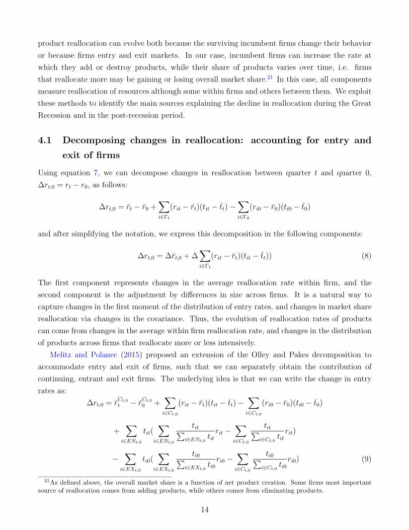
4.1 Decomposing changes in reallocation: accounting for entry and
exit of firms
Using equation 7, we can decompose changes in reallocation between quarter t and quarter 0,
�r
t,0 = r
t
� r0, as follows:
�r
t,0 = r
t
� r0 +X
i2�t
(rit
� r
t
)(tit
� t
t
)�X
i2�0
(ri0 � r0)(ti0 � t0)
and after simplifying the notation, we express this decomposition in the following components:
�r
t,0 = �r
t,0 +�X
i2�t
(rit
� r
t
)(tit
� t
t
)) (8)
The first component represents changes in the average reallocation rate within firm, and the
second component is the adjustment by di↵erences in size across firms. It is a natural way to
capture changes in the first moment of the distribution of entry rates, and changes in market share
reallocation via changes in the covariance. Thus, the evolution of reallocation rates of products
can come from changes in the average within firm reallocation rate, and changes in the distribution
of products across firms that reallocate more or less intensively.
Melitz and Polanec (2015) proposed an extension of the Olley and Pakes decomposition to
accommodate entry and exit of firms, such that we can separately obtain the contribution of
continuing, entrant and exit firms. The underlying idea is that we can write the change in entry
rates as:
�r
t,0 = r
Ct,0
t
� r
Ct,0
0 +X
i2Ct,0
(rit
� r
t
)(tit
� t
t
)�X
i2Ct,0
(ri0 � r0)(ti0 � t0)
+X
i2ENt,0
t
it
(X
i2ENt,0
t
itPi2ENt,0
t
it
r
it
�X
i2Ct,0
t
itPi2Ct,0
t
it
r
it
)
�X
i2EXt,0
t
i0(X
i2EXt,0
t
i0Pi2EXt,0
t
i0
r
i0 �X
i2Ct,0
t
i0Pi2Ct,0
t
i0
r
i0) (9)
21As defined above, the overall market share is a function of net product creation. Some firms most importantsource of reallocation comes from adding products, while others comes from eliminating products.
14
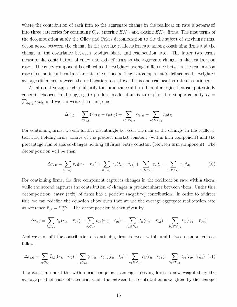
where the contribution of each firm to the aggregate change in the reallocation rate is separated
into three categories for continuing C
t,0, entering EN
t,0 and exiting EX
t,0 firms. The first terms of
the decomposition apply the Olley and Pakes decomposition to the the subset of surviving firms,
decomposed between the change in the average reallocation rate among continuing firms and the
change in the covariance between product share and reallocation rate. The latter two terms
measure the contribution of entry and exit of firms to the aggregate change in the reallocation
rates. The entry component is defined as the weighted average di↵erence between the reallocation
rate of entrants and reallocation rate of continuers. The exit component is defined as the weighted
average di↵erence between the reallocation rate of exit firms and reallocation rate of continuers.
An alternative approach to identify the importance of the di↵erent margins that can potentially
generate changes in the aggregate product reallocation is to explore the simple equality r
t
=P
i2�tr
it
t
it
, and we can write the changes as
�r
t,0 =X
i2Ct,0
(rit
t
it
� r
i0ti0) +X
i2ENt,0
r
it
t
it
�X
i2EXt,0
r
i0ti0
For continuing firms, we can further disentangle between the sum of the changes in the realloca-
tion rate holding firms’ shares of the product market constant (within-firm component) and the
percentage sum of shares changes holding all firms’ entry constant (between-firm component). The
decomposition will be then:
�r
t,0 =X
i2Ct,0
t
i0(rit � r
i0) +X
i2Ct,0
r
it
(tit
� t
i0) +X
i2ENt,0
r
it
t
it
�X
i2EXt,0
r
i0ti0 (10)
For continuing firms, the first component captures changes in the reallocation rate within them,
while the second captures the contribution of changes in product shares between them. Under this
decomposition, entry (exit) of firms has a positive (negative) contribution. In order to address
this, we can redefine the equation above such that we use the average aggregate reallocation rate
as reference r0,t =r0+rt
2. The decomposition is then given by
�r
t,0 =X
i2Ct,0
t
it
(rit
� r0,t)�X
i2Ct,0
t0,t(ri0 � r
t0) +X
i2ENt,0
t
it
(rit
� r0,t)�X
i2EXt,0
t
i0(ri0 � r0,t)
And we can split the contribution of continuing firms between within and between components as
follows
�r
t,0 =X
i2Ct,0
t
i,0t(rit�r
i0)+X
i2Ct,0
(ri,0t� r0,t)(tit�t
i0)+X
i2ENt,0
t
it
(rit
� r0,t)�X
i2EXt,0
t
i0(ri0� r0,t) (11)
The contribution of the within-firm component among surviving firms is now weighted by the
average product share of each firm, while the between-firm contribution is weighted by the average
15
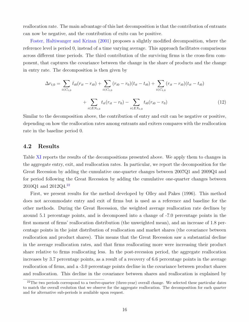
reallocation rate. The main advantage of this last decomposition is that the contribution of entrants
can now be negative, and the contribution of exits can be positive.
Foster, Haltiwanger and Krizan (2001) proposes a slightly modified decomposition, where the
reference level is period 0, instead of a time varying average. This approach facilitates comparisons
across di↵erent time periods. The third contribution of the surviving firms is the cross-firm com-
ponent, that captures the covariance between the change in the share of products and the change
in entry rate. The decomposition is then given by
�r
t,0 =X
i2Ct,0
t
i0(rit � r
i0) +X
i2Ct,0
(ri0 � r0)(tit � t
i0) +X
i2Ct,0
(rit
� r
i0)(tit � t
i0)
+X
i2ENt,0
t
it
(rit
� r0)�X
i2EXt,0
t
i0(ri0 � r0) (12)
Similar to the decomposition above, the contribution of entry and exit can be negative or positive,
depending on how the reallocation rates among entrants and exiters compares with the reallocation
rate in the baseline period 0.
4.2 Results
Table XI reports the results of the decompositions presented above. We apply them to changes in
the aggregate entry, exit, and reallocation rates. In particular, we report the decomposition for the
Great Recession by adding the cumulative one-quarter changes between 2007Q1 and 2009Q4 and
for period following the Great Recession by adding the cumulative one-quarter changes between
2010Q1 and 2012Q4.22
First, we present results for the method developed by Olley and Pakes (1996). This method
does not accommodate entry and exit of firms but is used as a reference and baseline for the
other methods. During the Great Recession, the weighted average reallocation rate declines by
around 5.1 percentage points, and is decomposed into a change of -7.0 percentage points in the
first moment of firms’ reallocation distribution (the unweighted mean), and an increase of 1.8 per-
centage points in the joint distribution of reallocation and market shares (the covariance between
reallocation and product shares). This means that the Great Recession saw a substantial decline
in the average reallocation rates, and that firms reallocating more were increasing their product
share relative to firms reallocating less. In the post-recession period, the aggregate reallocation
increases by 3.7 percentage points, as a result of a recovery of 6.6 percentage points in the average
reallocation of firms, and a -3.0 percentage points decline in the covariance between product shares
and reallocation. This decline in the covariance between shares and reallocation is explained by
22The two periods correspond to a twelve-quarter (three-year) overall change. We selected these particular datesto match the overall evolution that we observe for the aggregate reallocation. The decomposition for each quarterand for alternative sub-periods is available upon request.
16
the rebound of entry rates within firms followed by an even greater recovery in their exit rates.
Next, we implement the Melitz and Polanec (2015) methodology to further understand the
contributions of entry and exit of firms to product reallocation rates. The results suggest that
the decline of 5.1 percentage points in the weighted average product reallocation rate during the
Great Recession is partially accounted by a 1.4 percentage points increase in reallocation rate from
net entry of firms (which in its turn is further decomposed into 2.2 percentage points stemming
from the entry of products by entering firms, and -0.8 percentage points explained by the exit of
products by exiting firms). In the period following the Great Recession, net entry contributed 0.9
percentage points for the total 3.7 percentage points recovery in the aggregate product reallocation
rates.23 The decline in the importance of the net entry of firms in the post-recovery period indicates
that the recovery in reallocation was mainly driven by surviving incumbents firms, which seems
to be the group that was more dynamic in adjusting their reallocative behavior.
When we adapt the within and between decompositions of Griliches and Regev (1995) and
Foster, Haltiwanger and Krizan (2001) to the product reallocation rate, we obtain similar results for
the impact of entry and exit of firms. Moreover, we find relatively small di↵erences in the magnitude
of the within versus between components when we examine the impact of surviving incumbent
firms. Furthermore, we find that using these decomposition methods, reallocation by surviving
firms accounts for -6.4 percentage points of the decline in the weighted average reallocation rate
during the Great Recession, whereas the reallocation by surviving firms explains 2.8 percentage
points of the increase in reallocation rates in the post-recession period. The Griliches and Regev
(1995) decomposition shows that the decline in reallocation in the recession period resulted -7.9
percentage points from declines in the rate of product reallocation within surviving firms and 1.5
percentage points from variation between surviving firms. This decomposition suggests that among
surviving firms, the market share of high reallocation firms increased. The Foster, Haltiwanger
and Krizan (2001) decomposition assigns a larger negative contribution to the within component
(-10.8 percentage points), a negative component to the between firms reallocation (-1.4 percentage
points), and a sizable positive cross e↵ect (5.8 percentage points). This decomposition allows a
clear counterfactual exercise where changes in reallocation rates are calculated holding constant
product shares at their initial levels. Therefore, the above findings suggest that positive e↵ect of
between firms variation in explaining the decline in reallocation (obtained in all decompositions
with exception of Foster, Haltiwanger and Krizan (2001)) can result from the cross-term, i.e. the
relation between the change in shares and the change in reallocation rates.
Overall, the findings from this section show that the aggregate reallocation rate is largely
explained by the decisions to create and destroy products by incumbents firms, followed by the
contribution of entering and exiting firms. Moreover, the decompositions show that the decline in
23It is worth pointing out that the sign of the contribution of entry is always positive and the size of exit isalways negative, given that the reallocation rates of entering and exiting firms is by definition equal to 1, while forsurviving firms is closer to the level of 0.1.
17

reallocation result largely from declines in reallocation within surviving firms regardless of whether
we consider the recession or post-recession period. Finally, it is also clear from the Table XI, that
these results are not sensitive to the choice of decomposition method.
These results motivate us to better understand the consequences of reallocation within incum-
bent firms. We interpret these empirical facts as evidence that some of the variation of productivity
and growth within surviving firms documented in Foster, Haltiwanger and Syverson (2008) is re-
lated to how they manage heterogenous multi-product portfolios that are comprised of winners
(high revenue and high productivity products) and losers (low revenue and low productivity). In
section 6, we provide some suggestive evidence that the actions of firms to manage and reallocated
their product portfolio are associated with their subsequent productivity and revenue growth.
5 Product Reallocation and Innovation
What does product reallocation represent? In most models of creative destruction, output reallo-
cation plays an important role to determine productivity dynamics. These models emphasize that
adopting new products inherently involves the destruction of the old ones and that the pace at
which this takes place depends crucially on the innovation activities of the firm.24
In this section we establish that there is a positive relationship between product reallocation
and innovation. We implement two strategies to document that the addition and destruction of
products includes products that are truly innovative. First, we distinguish between two di↵erent
types of entry and exit – incremental and extensions– and document their evolution in the recession
and post recession period. We show that product extensions have characteristics that constitute
innovations within the firm. Second, we exploit the relationship between product creation and
destruction in the Nielsen data and R&D expenses available in Compustat. We show that firms
that invest more heavily in R&D present higher levels of reallocation. Both pieces of evidence
suggest that the measures of product entry and exit developed in the paper can be used as alter-
native proxies of innovation, with potential implications in testing the theories of how innovation
contributes to growth and cyclicality in the economy.
5.1 Exploring heterogeneous types of entry and exit
The results of the previous section do not distinguish products being added or destroyed in what
regards to how innovative they are. When we observe an entry of a new bar code, it may result
from a good that is very similar to others that the firms already has in its portfolio, or a good
that is truly unique and innovative. As discussed in Section 2 defining a product as an unique
barcode may rise some measurement concerns. In our dataset, small changes in packing or volume
24For example, in Aghion and Howitt (1992) firms get monopoly rents for their innovations until the next inno-vation arrives. In this case, the incentives for investing in innovation are substantial.
18
will likely result in a new bar code.25 This type of new products are not what researchers have
in mind when developing models of the e↵ect of innovation in reallocation. We address this issue
in two ways. First, we distinguish between two di↵erent types of innovation – incremental and
extensions– and we document their evolution in the recession and post recession period. Second,
we show that the results reported in the previous sections do not qualitatively change when we
consider coarser definitions of products.26
Under the first approach, our goal is to distinguish entry into new products within the main
product line of the firms, and new products beyond the main line of business of the firm. New
products that constitute only marginal changes in the stock of existing product, such as changes in
volume, and other minor characteristics of the products, are unlikely to involve a lot of resources
when developed and impact the outcomes of the firm in a significant way. On the contrary, new
products that are not within the core business of the firm, are likely to involve substantial changes
in the production technology with sizable consequences in the outcomes of the firm. We implement
a distinction between types of product by using the classification system of the Nielsen dataset. In
particular, we classify a new product in t as an improvement if the firm already has other products
of that type, i.e. if the firm in t � 1 already produces goods of the same module of the product
being created. We classify a new product as an extension if the new product is in a new module
to the firm.
We apply the same principle to classify exits by type. Exits are classified as improvements if the
firm maintain operations in that module. Exits are classified as extensions if they correspond to a
cessation of activity in that module. The distinction can help us understand if some products may
be terminated due to creative destruction (re- placed by new products within the same product
category) and those that were phased out due to the scaling down firms operations (products
without replacement).
Tables XII and XIII present the decomposition of aggregated and average entry and exit rate
by type over the period under analysis. For comparison, we also show the share of new and
exit products introduced by entrant and exit firms. As expected, most changes in barcode occur
within the same product module: around 80 percent of new barcodes and exit barcodes. Product
extensions correspond to 11 percent of all entries, exit extensions correspond to 14 percent of all
exits. Over the period under analysis, we observe that product extensions and shut downs of
product lines are more only slightly more cyclical than the entrants and exits of within firm’s
product lines. We interpret this as evidence that over the business cycle, firms change the rate at
which they make marginal changes in their stock of products, as well as the introduction of new
product lines.
25Broda and Weinstein (2010) also acknowledge that the their measures of product creation and destructioninclude changes in characteristics that may be secondary, and use information on the bar code characteristics fileto show that only a small part result from changes in size and flavor. We follow and alternative approach, more fitto our overall goal.
26See Section 2 for details.
19

Under the alternative definition of product, a good is the same if it shares the same brand within
the same product type (as defined by product module). Under this definition, we only identify
entry and exits that are clearly significant innovations from the perspective of the consumers.
Appendix D shows that the results we describe above on the aggregate reallocation rate and on
the impact of product reallocation on several innovation outputs remain very similar under this
specification.
5.2 Research and Development Expenses
In order to further understand the relation between firms’ innovation activities on the reallocation
of their products, we use the various measures of product creation and destruction described in the
previous section along with information of R&D expenses available in Compustat. This measure
is particularly relevant because, as it is defined by Compustat, it encompasses all planned search
aimed at the discovery of new knowledge that could lead to new products or the improvement of
the existing ones.
We begin by verifying that our Compustat-RMS sample represents well the various measures
of product entry and exit described in the previous section. Table VI shows that the entry rate,
reallocation rate, and exit rate are extremely close in both data sets. The firms in our matched
sample, nonetheless, sell on average more products and generate more revenue per year. To rule
out the possibility that firm size or other type of heterogeneity drives our results, in the analysis
that follows we control for an extended set of observables at the firm level. Given that our main
interest is to explore the determinants of reallocation within incumbent firms, we focus on studying
firms present in every period in our sample.27 Our specification is the following:
r
f,t+1 = ↵ + �R&Df,t
+ �Xf,t
+ µ
f
+ �
t
+ ✏
f,t
(13)
where rf,t
represents the reallocation rate of firm f in year t. R&D represents the ratio of research
and development expenses to total assets for firm f at time t. Our main focus is on � which
captures the direct impact of R&D on product reallocation. Xf,t
is a vector of firm level controls
that vary over time. All our specifications include year-e↵ects, �t
, to control for possible trends
and firm fixed e↵ects, µf
, to control for other types of heterogeneity.
Table XIV reports our results. Column (1) shows that R&D expenditures have a large positive
impact on reallocation after controlling for firm size; larger firms tend to engage in more R&D
activities. Next, we add a wide range of controls to disentangle the e↵ect of R&D from potentially
confounding firm-level factors. In column (2) we include the price cost margin and in column (3)
a control for firm idiosyncratic volatility. Our results do not vary under these specifications or if
measures of financial constraints are included (column (4)).28 This is not surprising given that even
27Our results are very similar if we study an unbalanced sample of firms and are available upon request.28The magnitude of the point estimate for � and its significance is not sensitive to including other measures of
20
without any time varying control the inclusion of both firm and time e↵ects account for more than
72% of all possible variation. In all cases the point estimates are large and statistically significant;
a hypothetical increase in R&D expenditures relative to sales of 1 percentage point increases the
reallocation rate by 1-1.5 percentage points. This is equivalent to an increase of close to 15% in
the reallocation rate.29
6 Reallocation and Growth of Firm
Our findings so far strongly suggest that the innovation e↵orts of the firms are associated with
higher reallocation rates. The second key prediction of Schumpeterian growth models to test is
whether increases in the reallocation rate of products lead to larger growth rates of firms and
improvements in the products they produce.
6.1 Reallocation and Revenue Growth
We first confirm the prediction on revenue growth by estimating the following equation in the data:
Revenuef,t+1 = ↵ + � r
f,t
+ �Xf,t
+ µ
f
+ �
t
+ ✏
f,t
(14)
where Revenuef,t
is the sum of the revenue of all products in the firm’s portfolio at time t. As
before, all our specifications include both firm and time fixed e↵ects and consider only a balanced
sample of firms.30 Furthermore, given that in order to run this specification we only require the
information available in the RMS, equation 14 is estimated using quarterly data.
Column (1) in table XVI shows that �, our coe�cient of interest, is both economically and
statistically significant. This is after controlling for revenue in the previous period. The table also
shows that, not surprisingly, most of the revenue growth due to reallocation of products comes
from the entry margin. The exit rate on the other hand is negatively related to the revenue growth
in the next quarter.
At the entry margin, entry of products in the module where a firm operated before, Column
(3) in the table, and entry of products in a new module, Column (4), are associated with revenue
growth by similar magnitudes. At the exit margin, closing down a product module completely,
Column (7), is more strongly correlated with revenue growth, compared to destructing products in
the module they keep operating (related to the idea of Creative Destruction), Column (6). We get
financial constraints such as the firm’s S&P long-term issuer rating.29When we study the entry and exit rates separately, we find that most of the correlation comes from the entry
margin. However, consistent with the prediction of Schumpeterian growth models, R&D is strongly correlated withboth entry and exit when we examine their patterns within the main product module of the firm; exactly where weexpect to see older varieties being replaced by newer and better products.
30Summary statistics of quarterly firm-level revenue for the balanced sample is reported in Table XV
21

consistent results with two other specifications, i) with full sample and ii) using brands as product,
as shown in Table A.XII and A.XIII.
6.2 Reallocation and Quality Improvements
A similar analysis can be done to explore whether higher reallocation rates lead to increases in the
average quality of firms’ portfolios. Several growth models, such as those in Klette and Kortum
(2004) and Lentz and Mortensen (2008), predict that higher quality versions of a product are the
outcome of the innovation activities of the firms. To study these predictions we use three di↵erent
measures to approximate product quality: relative prices, a percentile-based measure, and per-
ceived quality measure.
Benchmark Quality To measure quarterly firm-level average product quality, we use prices
as proxy for quality as Argente and Lee (2016). This measure is similar to those used in the
international trade literature where, if a sector or firm in country is able to export a large volume
at a high price, then it must be producing high-quality goods (Hummels and Klenow, 2005; Hallak
and Schott, 2011; Kugler and Verhoogen, 2012). As a benchmark measure, we proxy product
quality by the average relative price of the barcode-level good within each product category. First,
we measure the log-di↵erence between the price of good j and the median price for category c in
quarter t.
R
benchmarkjt
= logP
jt
P
ct
where R
benchmarkjt
is the relative price and P
ct
is the median price of category c. Therefore, if the
price of a high quality type of milk, say organic milk, is much higher than the median price of
milk, then R
benchmarkjt
is positive and high.
We then calculate firm-level average quality by combining information on product-level quality
and product portfolio of each firm. The average product quality of firm f is:
Q
benchmarkft
=X
jf
!
jft
R
benchmarkjt
where !
jft
is a revenue weight. Q
benchmarkft
captures how far the prices of the products produced
by firm f are from the median price level in each of their categories at time t.
Percentile-based Quality Measure Since the cross-sectional distribution of prices in a given
category is fat-tailed, a cardinal measure of quality may be noisy and thus problematic. For this
reason, we also define a percentile-based measure of quality as follows:
22

R
percentilejt
=1
N
ct
(njct
� 1
2)
where N
jt
is total number of products in category c at quarter t and n
jt
is an ordinal rank of
product j. Q
percentileft
can be defined as before by aggregating the product portfolio of each firm
using revenue weights.
Perceived Quality Measure from Demand Estimation (work in progress)
The estimation of our final quality measure begins with the demand specification in Hottman,
Redding and Weinstein (2016). We then estimate the elasticity of substitution using an instrumen-
tal variable approach and back out the product specific perceived quality from system (Gervais,
2015; Piveteau and Smagghue, 2015; Fieler, Eslava and Xu, 2016). We derive the following equation
from the nested constant elasticity of substitution utility system described in Appendix D.
� log(Cufmct
) = �
fmct
� �� log(Pufmct
) + (� � 1)'u
+ ✏
ufmct
(15)
where Pufmct
is an average price of product u of firm f in module m at local market c at time t. To
address the standard simultaneity concern that taste shocks in the error term are correlated with
observed price changes, we follow Beraja, Hurst and Ospina (2016) and Fally and Faber (2017)
and instrument for local consumer price changes across products � logPufmct
with national-level
leave-out mean price changes: 1N�1
⌃j 6=c
� logPufmjt
.
In the current version of the paper, we estimate an elasticity of substitution � for each product
module, using a smaller version of the scanner data, the Nielsen Homescan Panel data (HMS).
Table XVII reports the estimated elasticities of substitution. For 80 percent of modules, our
IV estimates are statistically significant at the 1 percent level. On average, the module specific
elasticity of substitution is 3.62; we find the OLS estimates to be upward biased. Furthermore,
we find our perceived quality measures to be positively correlated with our benchmark quality
measure.31
Using these quality measures, we now test association between our measure of product reallo-
cation and firm-level average product quality improvement. We use the following specification:
Q
f,t+1 = ↵ + � r
f,t
+ �Xf,t
+ µ
f
+ �
t
+ ✏
f,t
(16)
where f is the firm, and t is the quarter. Our main focus is on � which captures the direct impact
of reallocation on firm-level average product quality in the next quarter. X
f,t
is a vector of firm
level controls, µf
represents firm fixed e↵ects and �
t
represents time e↵ects. By construction, the
benchmark quality measure is centered at 0 and the percentile-based quality measure is center at
31Mean correlation is 0.54 with standard deviation 0.21. In a subsequent version of the paper, we plan to estimateperceived quality measures using the RMS and check the robustness of our regression results that follow.
23
50.32 Table XVIII reports the relationship between our reallocation measures and our benchmark
quality measure, Qbenchmarkf,t+1 . We again keep balanced panel of firms to investigate the importance
of reallocation among surviving firms. An increase in reallocation is associated with quality im-
provements in the following quarter. This correlation is mainly driven by the entry margin of
products. Large firms tend to produce higher quality products on average. Furthermore, as shown
in columns (3)-(4), quality improves more for product extensions beyond the module than for
incremental innovations. Our results are consistent in two other specifications, with full sample,
or using brands as product, shown in Table A.XIV and A.XV.33
6.3 Reallocation and Productivity
The remaining central implication of models with creative destruction to be tested is whether the
reallocation of products is a major source of productivity growth. This prediction has been hard
to examine directly in the data given the lack of availability of datasets combining both product
and firm level information.34
We begin by computing total factor productivity in the Compustat data relying primarily
on the methodology developed by Imrohoroglu and Tuzel (2014). We then regress the natural
logarithm of TFP on the annual reallocation rate as follows:
TFP
f,t+1 = ↵ + � r
f,t
+ �Xf,t
+ µ
f
+ �
t
+ ✏
f,t
(17)
where as before f is the firm, and t is the year. Our main focus is once again on � which captures
the direct impact of reallocation on firm productivity. Table XIX reports our results. Column (1)
shows that both variables are strongly correlated even after controlling for the size of the firm. This
is important because in general larger firms have higher productivity and, as we have shown, they
also have higher rate of reallocation. Column (2) includes controls for market power by including
the price-to-cost margin as control. Column (3) includes the standard deviation of sales to control
for the possibility that firms with faster sales growth have higher rates of product entry and exit.
Lastly, in column (4) we control for di↵erences in financial constraints across firms by including
the Kaplan-Zingales index. Our estimates of � remain very similar across specifications and show
that, on average, an increase of 5 percentage points in reallocation increases TFP between 0.9 and
1%.
When we examine the contribution of entries and exits separately, we find that the contribution
of reallocation to TFP mainly comes from exits. But, interestingly, when we explore improvements
32As shown in Table XV, a balanced sample of firms has an average benchmark quality above 0 and an averagepercentile-based quality of above 50. This is because short-lived firms in our sample are on average low-qualityproducers.
33The results are also robust to a percentile based quality measure, which is available upon request.34This question has been, nonetheless, explored in other contexts such as the reallocation of establishments
(Bartelsman and Doms, 2000; Foster, Haltiwanger and Krizan, 2001; Foster, Grim and Haltiwanger, 2016). In bothcases, a large share of productivity growth can be explained by the reallocation of resources.
24
and extensions separately. We find that product extensions, those products who are more likely
to involve a larger innovation but are less common in our data, have a positive and significant
contribution to TFP. On the other hand, exits within the main module of the firm, those that are
more likely to come from replacing outdated products for better products, contribute positively
and significantly to TFP.
6.4 Summary of Results and Implications
The importance of product reallocation has been central in models of creative destruction for
decades but, as the theoretical literature has evolved, the lack of data availability made many of its
central implications hard to be tested. Our calculations validate many predictions of these models.
First, we find that faster innovation-led growth is associated with higher rates of reallocation of
products (Aghion, Akcigit and Howitt, 2014). Product reallocation is positively related to R&D
and to revenue growth. Second, although both entrants and incumbents innovate (Bartelsman and
Doms, 2000), most growth appears to come from incumbents improving existing varieties (Garcia-
Macia, Hsieh and Klenow, 2016; Acemoglu and Cao, 2015). Third, small firms and new entrants
have a comparative advantage for achieving major innovations or, as we called them within the
context of the consumer goods sector, extensions (Akcigit and Kerr, 2010). And, lastly, a more
innovative firm has higher levels of productivity (Lentz and Mortensen, 2008).
How much of the decrease in aggregate productivity can be attributed to changes in the product
reallocation? Our baseline estimate of column 1 in Table XIX suggests that total factor productiv-
ity increases by approximately 0.2 percent for every 1 percentage point increase in reallocation.35
Given that the reallocation rate decreased by more than 4 percentage points during the recession
and that TFP declined almost 5% from 2007 to 2010 in our data, product reallocation can explain
15-20% of the total decline in total factor productivity. This suggests that a significant drop in
aggregate productivity was driven by firms slowing down their innovation activities during this
period. This, in turn, decreased the dynamism in which they replaced older products for improved
products decreasing the pace of quality improvements and ultimately economic growth.
7 Conclusion
This paper describes the extent of product innovation and reallocation in the consumer good sector
over the period 2006-2014. We find 30 percent decline in product reallocation during the Great
Recession, and investigate the impact of this drop on firm-level outcomes such as revenue, product
quality, and total productivity. The analysis provides several findings. First, product reallocation
35The interpretation of our results should consider the fact that they were computed using a sample of largepublicly traded firms. Moreover, although within firm reallocation is by far the most important component of theoverall reallocation rate, our estimates in section 6.3 ignore the contribution of firm entry and exit.
25

is strongly pro-cyclical and the cyclical pattern is overwhelmingly a consequence of within firm
reallocation. Second, the rate of product reallocation is strongly related to the innovation e↵orts
of the firms. Third, firms that have higher reallocation rates grow faster, launch higher quality
goods, and experience larger gains in productivity.
Given that higher reallocation activities lead firms to grow both quantitatively and qualitatively,
the fact that its pace su↵ered an important drop had substantial implications for aggregate growth
in this period. More importantly, the fact that the reallocation rate took so long to return to its
pre-recession level suggests it was an important factor in the slow recovery the economy experienced
after the Great Recession. Our findings also suggest that industrial and innovation policies aimed
at increasing economic growth should contemplate the relative importance of the product-mix
decisions. This is particularly relevant for incumbent firms as they account to the majority of the
decline in dynamism in the retail sector that ultimately led to important declines in total factor
productivity.
26

References
Acemoglu, Daron and Dan Cao, “Innovation by entrants and incumbents,” Journal of Economic
Theory, 2015, 157, 255–294.
, Ufuk Akcigit, Nicholas Bloom, and William R Kerr, “Innovation, Reallocation and Growth,”
NBER Working Paper No. 18993, 2013.
Aghion, Philippe and Peter Howitt, “A Model of Growth through Creative Destruction,” Econo-
metrica, 1992, 60 (2), 323–351.
, Ufuk Akcigit, and Peter Howitt, “What Do We Learn from Schumpeterian Growth Theory?,”
in Philippe Aghion and Steven N Durlauf, eds., Handbook of Economic Growth, Vol. 2, Oxford:
North Holland, 2014, chapter 1, pp. 515–563.
Akcigit, Ufuk andWilliam R Kerr, “Growth Through Heterogeneous Innovations,” NBER Working
Paper No. 16443, 2010.
Argente, David and Chen Yeh, “Price-Setting under Uncertain Demand: A Menu Cost Model with
Price Experimentation,” 2016.
and Munseob Lee, “Cost of Living Inequality during the Great Recession,” 2016.
Bartelsman, Eric J and Mark Doms, “Understanding productivity: Lessons from longitudinal
microdata,” Journal of Economic literature, 2000, 38 (3), 569–594.
Beraja, Martin, Erik Hurst, and Juan Ospina, “The Aggregate Implications of Regional Business
Cycles,” NBER Working Paper No. 21956, 2016.
Bernard, Andrew B, Stephen J Redding, and Peter K Schott, “Multiple-Product Firms and Prod-
uct Switching,” American Economic Review, 2010, 100 (1), 70–97.
Broda, Christian and David E Weinstein, “Product Creation and Destruction: Evidence and Price
Implications,” American Economic Review, 2010, 100 (3), 691–723.
Caballero, Ricardo J and Mohamad L Hammour, “The Cleansing E↵ect of Recessions,” American
Economic Review, 1994, 84 (5), 1350–68.
Chevalier, Judith A, Anil K Kashyap, and Peter E Rossi, “Why Don’t Prices Rise During Periods
of Peak Demand? Evidence from Scanner Data,” American Economic Review, 2003, 93 (1),
15–37.
Davis, Steven J and John Haltiwanger, “Gross Job Creation, Gross Job Destruction, and Employ-
ment Reallocation,” Quarterly Journal of Economics, 1992, 107 (3), 819–863.
27

and , “Labor Market Fluidity and Economic Performance,” NBER Working Paper No. 20479,
2014.
, John C Haltiwanger, and Scott Schuh, “Job creation and destruction,” MIT Press Books, 1996.
Decker, Ryan, John Haltiwanger, Ron Jarmin, and Javier Miranda, “The Role of Entrepreneurship
in U.S. Job Creation and Economic Dynamism,” Journal of Economic Perspectives, 2014, 28
(3), 3–24.
Fally, Thibault and Benjamin Faber, “Firm Heterogeneity in Consumption Baskets: Evidence from
Home and Store Scanner Data,” NBER Working Paper No. 23101, 2017.
Fieler, Ana Cecılia, Marcela Eslava, and Daniel Yi Xu, “Trade, Quality Upgrading, and Input
Linkages: Theory and Evidence from Colombia,” 2016.
Foster, Lucia, Cheryl Grim, and John Haltiwanger, “Reallocation in the Great Recession: Cleans-
ing or Not?,” Journal of Labor Economics, 2016, 34 (S1), S293–S331.
, John Haltiwanger, and Chad Syverson, “Reallocation, firm turnover, and e�ciency: Selection
on productivity or profitability?,” American economic review, 2008, 98 (1), 394–425.
, , and Cornell J Krizan, “Aggregate Productivity Growth. Lessons from Microeconomic
Evidence,” in “New Developments in Productivity Analysis,” University of Chicago Press, 2001,
pp. 303–372.
, , and , “Market Selection, Reallocation, and Restructuring in the U.S. Retail Trade Sector
in the 1990s,” Review of Economics and Statistics, 2006, 88 (4), 748–758.
Garcia-Macia, Daniel, Chang-Tai Hsieh, and Peter J Klenow, “How Destructive is Innovation?,”
2016.
Gervais, Antoine, “Product quality and firm heterogeneity in international trade,” Canadian Jour-
nal of Economics, 2015, 48 (3), 1152–1174.
Gorodnichenko, Yuriy and Michael Weber, “Are sticky prices costly? Evidence from the stock
market,” American Economic Review, 2016, 106 (1), 165–199.
Gourio, Francois and Michael Siemer, “A Missing Generation of Firms? Aggregate E↵ects of the
Decline in New Business Formation,” 2014.
Griliches, Zvi and Haim Regev, “Firm Productivity in Israeli Industry 1979–1988,” Journal of
Econometrics, 1995, 65 (1), 175–203.
Grossman, Gene M and Elhanan Helpman, “Quality ladders in the theory of growth,” The Review
of Economic Studies, 1991, 58 (1), 43–61.
28
Hallak, Juan Carlos and Peter K Schott, “Estimating Cross-Country Di↵erences in Product Qual-
ity,” Quarterly Journal of Economics, 2011, 126 (1), 417–474.
Hottman, Colin J, Stephen J Redding, and David E Weinstein, “Quantifying the sources of firm
heterogeneity,” Quarterly Journal of Economics, 2016, 131 (3), 1291–1364.
Hummels, David and Peter J Klenow, “The Variety and Quality of a Nation’s Exports,” American
Economic Review, 2005, 95 (3), 704–723.
Imrohoroglu, Ayse and Selale Tuzel, “Firm-level productivity, risk, and return,” Management
Science, 2014, 60 (8), 2073–2090.
Kaplan, Greg and Guido Menzio, “The Morphology of Price Dispersion,” NBER Working Paper
No. 19877, 2014.
Kaplan, Steven N and Luigi Zingales, “Do investment-cash flow sensitivities provide useful mea-
sures of financing constraints?,” Quarterly Journal of Economics, 1997, 112 (1), 169–215.
Klette, Tor Jakob and Samuel Kortum, “Innovating Firms and Aggregate Innovation,” Journal of
Political Economy, 2004, 112 (5).
Kugler, Maurice and Eric Verhoogen, “Prices, Plant Size, and Product Quality,” Review of Eco-
nomic Studies, 2012, 79 (1), 307–339.
Lentz, Rasmus and Dale T Mortensen, “An empirical model of growth through product innova-
tion,” Econometrica, 2008, 76 (6), 1317–1373.
Melitz, Marc J and Saso Polanec, “Dynamic Olley-Pakes Productivity Decomposition with Entry
and Exit,” Rand Journal of Economics, 2015, 46 (2), 362–375.
Moreira, Sara, “Firm Dynamics, Persistent E↵ects of Entry Conditions, and Business Cycles,”
2016.
Olley, G. Steven and Ariel Pakes, “The Dynamics of Productivity in the Telecommunications
Equipment Industry,” Econometrica, 1996, 64 (6), 1263–1297.
Piveteau, Paul and Gabriel Smagghue, “Estimating Firm Product Quality using Trade Data,”
2015.
Schoenle, Raphael, “International Menu Costs and Price Dynamics,” Review of International Eco-
nomics, 2016.
29
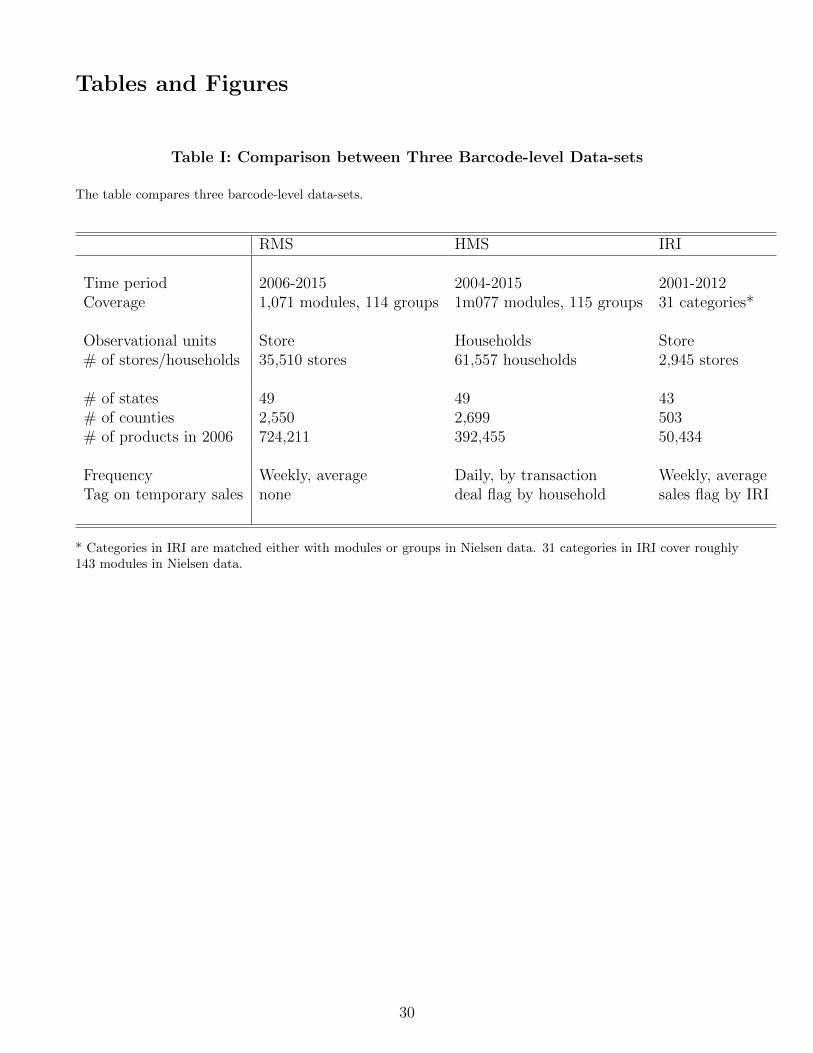
Tables and Figures
Table I: Comparison between Three Barcode-level Data-sets
The table compares three barcode-level data-sets.
RMS HMS IRI
Time period 2006-2015 2004-2015 2001-2012Coverage 1,071 modules, 114 groups 1m077 modules, 115 groups 31 categories*
Observational units Store Households Store# of stores/households 35,510 stores 61,557 households 2,945 stores
# of states 49 49 43# of counties 2,550 2,699 503# of products in 2006 724,211 392,455 50,434
Frequency Weekly, average Daily, by transaction Weekly, averageTag on temporary sales none deal flag by household sales flag by IRI
* Categories in IRI are matched either with modules or groups in Nielsen data. 31 categories in IRI cover roughly143 modules in Nielsen data.
30

Table II: Top 20 Firms in Total Revenue
The table reports top 20 firms in total revenue for 2006-2014. The total revenue is in billion USD.
Ranking Name of Firm Total Revenue
1 Procter & Gamble Company 87.172 General Mills, Inc. 34.093 Kraft Foods, Inc. 33.684 Nestle USA Inc. 29.485 Frito-Lay Company 29.336 Coca-Cola USA Operations 27.367 Philip Morris USA/Tobacco Products 25.908 Pepsi-Cola North America Inc. 24.559 Kimberly-Clark/Household Products Div. 18.8210 Anheuser-Busch InBev 17.0211 Kellogg Company 16.7012 Unilever Home and Personal Care USA 16.2713 The Hershey Company 15.4114 Nabisco Biscuit Company 14.8915 ConAgra Foods Inc. 14.8916 Campbell Soup Company 14.6017 Produce Marketing Association Inc. 13.9718 Dr. Pepper/Seven Up, Inc. 12.3019 Oscar Mayer Foods Corp. 12.1820 Nestle Purina PetCare Company 11.67
31

Table III: Summary Statistics of Products
The table shows summary statistics of products.
2007-2013 2007 2010 2013
Number of products 251032 227249 241811 296527
By status (share of products)Entrants 0.019 0.052 0.032 0.042Exits 0.014 0.035 0.035 0.046
By diversification (average)Per module 284 587 575 593Per group 2770 5506 5397 5559Per department 31856 62769 61526 63376
By Revenue (share of products)[0,104[ 0.600 0.617 0.598 0.629[104,105[ 0.220 0.228 0.233 0.216[105,106[ 0.131 0.130 0.139 0.130>=106 0.049 0.025 0.029 0.025
32

Table
IV:Summary
StatisticsofFirmsin
theData
Thetable
show
ssummarystatistics
offirm
sin
thedata.
Byrevenu
e,wereportshareof
continuingfirm
s.
2007-2013
2007
2010
2013
Number
offirm
s(average)
14068
13952
13611
15305
Bystatus(shareof
firm
s)Entrants
0.022
0.028
0.017
0.026
Exits
0.018
0.021
0.015
0.019
Con
tinu
ersExp
anding
0.129
0.134
0.115
0.147
Con
tinu
ersCon
tracting
0.125
0.136
0.120
0.119
Bydiversification
SingleProduct
Shareof
firm
s0.259
0.275
0.257
0.246
MultiProduct
&SingleMod
ule
Shareof
firm
s0.260
0.255
0.261
0.261
Meannu
mber
ofproducts
5.7
5.6
5.6
5.7
Mediannu
mber
ofproducts
33
33
MultiMod
ule
&SingleGroup
Shareof
firm
s0.123
0.118
0.124
0.127
Meannu
mber
ofproducts
13.6
12.8
13.8
14.1
Mediannu
mber
ofproducts
77
77
MultiGroup&
SingleDepartm
ent
Shareof
firm
s0.197
0.193
0.197
0.200
Meannu
mber
ofproducts
25.3
23.2
25.4
27.7
Mediannu
mber
ofproducts
1010
1110
MultiDepartm
ent
Shareof
firm
s0.162
0.160
0.161
0.167
Meannu
mber
ofproducts
58.5
54.1
58.1
61.9
Mediannu
mber
ofproducts
1615
1617
ByRevenue(shareof
firm
s)[0,104[
0.443
0.459
0.433
0.451
[104,105[
0.266
0.260
0.271
0.263
[105,106[
0.190
0.187
0.192
0.184
>=10
60.102
0.094
0.104
0.102
33
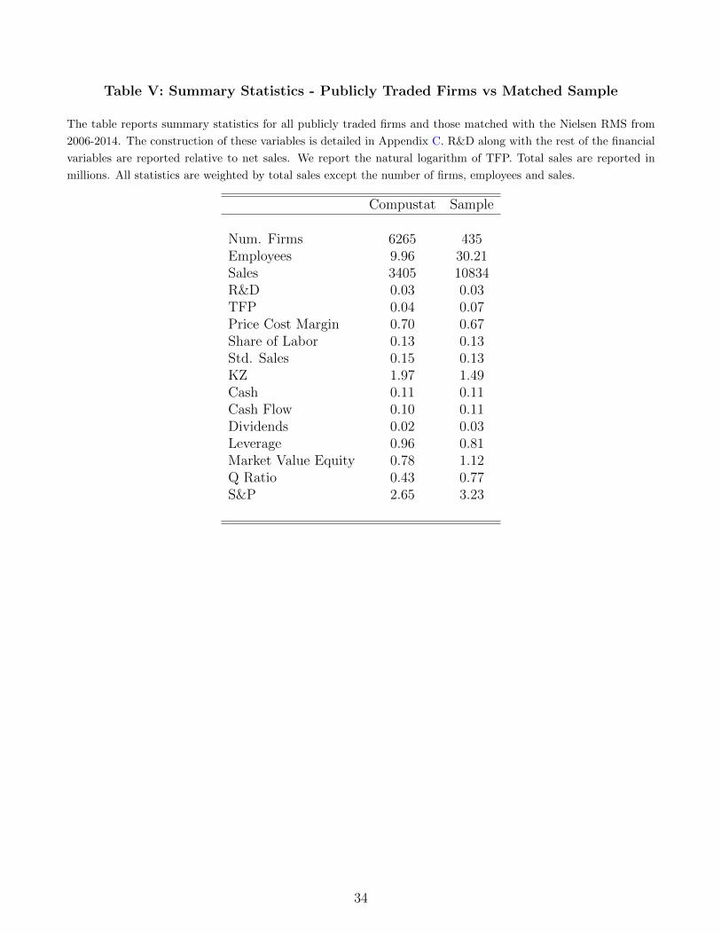
Table V: Summary Statistics - Publicly Traded Firms vs Matched Sample
The table reports summary statistics for all publicly traded firms and those matched with the Nielsen RMS from
2006-2014. The construction of these variables is detailed in Appendix C. R&D along with the rest of the financial
variables are reported relative to net sales. We report the natural logarithm of TFP. Total sales are reported in
millions. All statistics are weighted by total sales except the number of firms, employees and sales.
Compustat Sample
Num. Firms 6265 435Employees 9.96 30.21Sales 3405 10834R&D 0.03 0.03TFP 0.04 0.07Price Cost Margin 0.70 0.67Share of Labor 0.13 0.13Std. Sales 0.15 0.13KZ 1.97 1.49Cash 0.11 0.11Cash Flow 0.10 0.11Dividends 0.02 0.03Leverage 0.96 0.81Market Value Equity 0.78 1.12Q Ratio 0.43 0.77S&P 2.65 3.23
34
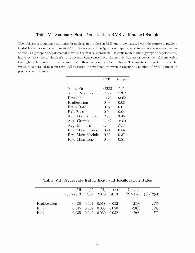
Table VI: Summary Statistics - Nielsen RMS vs Matched Sample
The table reports summary statistics for all firms in the Nielsen RMS and those matched with the sample of publicly
traded firms in Compustat from 2006-2014. Average modules (groups or departments) indicates the average number
of modules (groups or departments) in which the firm sells products. Revenue main module (groups or departments)
indicates the share of the firm’s total revenue that comes from the module (groups or departments) from which
the highest share of its revenue comes from. Revenue is reported in millions. The construction of the rest of the
variables is detailed in main text. All statistics are weighted by revenue except the number of firms, number of
products and revenue.
RMS Sample
Num. Firms 37282 505Num. Products 16.99 213.2Revenue 1.170 33.62Reallocation 0.08 0.08Entry Rate 0.07 0.07Exit Rate 0.04 0.04Avg. Departments 2.78 3.45Avg. Groups 12.62 18.50Avg. Modules 42.96 57.11Rev. Main Group 0.71 0.55Rev. Main Module 0.52 0.37Rev. Main Dept. 0.88 0.81
Table VII: Aggregate Entry, Exit, and Reallocation Rates
All (1) (2) (3) Change2007-2013 2007 2010 2013 (2)/(1)-1 (3)/(2)-1
Reallocation 0.080 0.094 0.068 0.082 -28% 21%Entry 0.045 0.052 0.038 0.050 -28% 32%Exit 0.035 0.042 0.030 0.032 -29% 7%
35
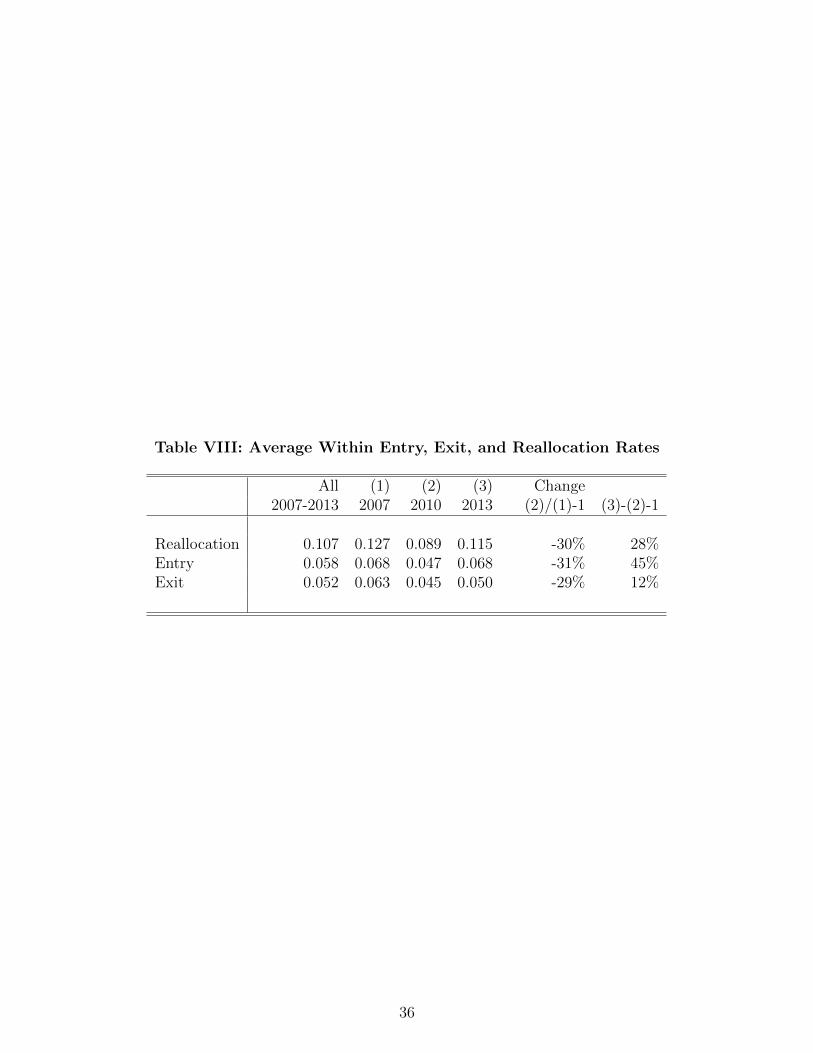
Table VIII: Average Within Entry, Exit, and Reallocation Rates
All (1) (2) (3) Change2007-2013 2007 2010 2013 (2)/(1)-1 (3)-(2)-1
Reallocation 0.107 0.127 0.089 0.115 -30% 28%Entry 0.058 0.068 0.047 0.068 -31% 45%Exit 0.052 0.063 0.045 0.050 -29% 12%
36

Table IX: Aggregate Reallocation by Types of Firms
All (1) (2) (3) Change2007-2013 2007 2010 2013 (2)/(1)-1 (3)-(2)-1
ReallocationExpanding Entrant 0.003 0.004 0.002 0.003 -45% 52%Expanding Incumbent 0.045 0.049 0.037 0.051 -25% 37%Contracting Exit 0.001 0.002 0.001 0.001 -37% 32%Contracting Incumbent 0.027 0.035 0.025 0.023 -30% -8%Unchanged Incumbent 0.004 0.004 0.003 0.004 -33% 29%
EntryExpanding Entrant 0.003 0.004 0.002 0.003 -45% 52%Expanding Incumbent 0.036 0.038 0.030 0.040 -22% 36%Contracting Incumbent 0.005 0.008 0.005 0.004 -42% -7%Unchanged Incumbent 0.002 0.002 0.001 0.002 -33% 28%
ExitExpanding Incumbent 0.010 0.011 0.007 0.010 -34% 42%Contracting Exit 0.001 0.002 0.001 0.001 -37% 32%Contracting Incumbent 0.022 0.027 0.020 0.019 -26% -8%Unchanged Incumbent 0.002 0.002 0.001 0.002 -33% 31%
ReallocationQ1 revenue 0.005 0.008 0.003 0.005 -55% 58%Q2 revenue 0.006 0.007 0.005 0.007 -31% 48%Q3 revenue 0.011 0.013 0.009 0.011 -32% 28%Q4 revenue 0.057 0.065 0.049 0.056 -24% 15%
Q1 revenue only incumbents 0.002 0.002 0.001 0.002 -44% 74%Q2 revenue only incumbents 0.004 0.005 0.003 0.004 -43% 31%Q3 revenue only incumbents 0.009 0.012 0.008 0.008 -35% 6%Q4 revenue only incumbents 0.049 0.058 0.042 0.047 -27% 12%
EntryQ1 revenue 0.002 0.003 0.002 0.003 -47% 100%Q2 revenue 0.003 0.004 0.003 0.005 -33% 77%Q3 revenue 0.006 0.007 0.005 0.007 -36% 48%Q4 revenue 0.032 0.036 0.028 0.033 -24% 21%
Q1 revenue only incumbents 0.001 0.001 0.001 0.001 -33% 106%Q2 revenue only incumbents 0.002 0.003 0.001 0.002 -48% 59%Q3 revenue only incumbents 0.005 0.007 0.004 0.005 -41% 16%Q4 revenue only incumbents 0.028 0.032 0.024 0.027 -27% 17%
ExitQ1 revenue 0.002 0.004 0.002 0.002 -61% 18%Q2 revenue 0.003 0.003 0.002 0.003 -28% 16%Q3 revenue 0.005 0.005 0.004 0.004 -26% 5%Q4 revenue 0.024 0.028 0.021 0.023 -25% 6%
Q1 revenue only incumbents 0.001 0.001 0.001 0.001 -53% 36%Q2 revenue only incumbents 0.002 0.002 0.001 0.001 -36% 4%Q3 revenue only incumbents 0.004 0.005 0.004 0.004 -27% -4%Q4 revenue only incumbents 0.021 0.026 0.019 0.020 -27% 6%
ReallocationSingle-product 0.002 0.003 0.002 0.002 -43% 14%Single-Module 0.007 0.008 0.005 0.007 -30% 23%Single-Group 0.008 0.009 0.007 0.007 -19% 1%Single-Department 0.020 0.023 0.017 0.022 -26% 28%Multi-department 0.040 0.047 0.034 0.040 -29% 19%
EntrySingle-product 0.001 0.002 0.001 0.001 -49% 37%Single-Module 0.003 0.004 0.003 0.004 -33% 41%Single-Group 0.004 0.005 0.004 0.004 -13% 3%Single-Department 0.011 0.012 0.009 0.013 -19% 37%Multi-department 0.022 0.026 0.018 0.024 -30% 32%
ExitSingle-product 0.001 0.002 0.001 0.001 -38% -5%Single-Module 0.003 0.004 0.003 0.003 -26% 5%Single-Group 0.004 0.004 0.003 0.003 -25% -2%Single-Department 0.009 0.011 0.008 0.009 -33% 18%Multi-department 0.018 0.021 0.016 0.016 -27% 5%
37
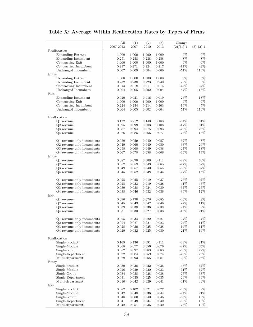
Table X: Average Within Reallocation Rates by Types of Firms
All (1) (2) (3) Change2007-2013 2007 2010 2013 (2)/(1)-1 (3)-(2)-1
ReallocationExpanding Entrant 1.000 1.000 1.000 1.000 0% 0%Expanding Incumbent 0.251 0.258 0.238 0.258 -8% 8%Contracting Exit 1.000 1.000 1.000 1.000 0% 0%Contracting Incumbent 0.237 0.271 0.224 0.217 -17% -3%Unchanged Incumbent 0.007 0.009 0.004 0.009 -57% 116%
EntryExpanding Entrant 1.000 1.000 1.000 1.000 0% 0%Expanding Incumbent 0.232 0.238 0.223 0.240 -6% 8%Contracting Incumbent 0.014 0.018 0.011 0.015 -42% 37%Unchanged Incumbent 0.004 0.005 0.002 0.004 -57% 116%
ExitExpanding Incumbent 0.020 0.021 0.016 0.019 -26% 18%Contracting Exit 1.000 1.000 1.000 1.000 0% 0%Contracting Incumbent 0.224 0.254 0.214 0.203 -16% -5%Unchanged Incumbent 0.004 0.005 0.002 0.004 -57% 116%
ReallocationQ1 revenue 0.172 0.212 0.140 0.183 -34% 31%Q2 revenue 0.095 0.099 0.083 0.108 -17% 31%Q3 revenue 0.087 0.094 0.075 0.093 -20% 23%Q4 revenue 0.076 0.085 0.066 0.077 -23% 18%
Q1 revenue only incumbents 0.050 0.059 0.040 0.057 -32% 43%Q2 revenue only incumbents 0.049 0.060 0.040 0.050 -33% 26%Q3 revenue only incumbents 0.058 0.068 0.049 0.058 -27% 18%Q4 revenue only incumbents 0.067 0.078 0.058 0.066 -26% 14%
EntryQ1 revenue 0.087 0.098 0.069 0.111 -29% 60%Q2 revenue 0.052 0.059 0.043 0.065 -27% 52%Q3 revenue 0.049 0.057 0.040 0.055 -30% 37%Q4 revenue 0.045 0.052 0.038 0.044 -27% 15%
Q1 revenue only incumbents 0.025 0.025 0.019 0.037 -25% 97%Q2 revenue only incumbents 0.025 0.033 0.019 0.028 -41% 43%Q3 revenue only incumbents 0.030 0.038 0.024 0.030 -37% 25%Q4 revenue only incumbents 0.038 0.046 0.032 0.036 -30% 12%
ExitQ1 revenue 0.096 0.130 0.078 0.085 -40% 8%Q2 revenue 0.045 0.043 0.042 0.046 -2% 11%Q3 revenue 0.039 0.038 0.036 0.039 -4% 8%Q4 revenue 0.031 0.033 0.027 0.033 -16% 21%
Q1 revenue only incumbents 0.025 0.034 0.022 0.021 -37% -4%Q2 revenue only incumbents 0.024 0.027 0.021 0.023 -24% 11%Q3 revenue only incumbents 0.028 0.030 0.025 0.028 -14% 11%Q4 revenue only incumbents 0.029 0.032 0.025 0.030 -21% 16%
ReallocationSingle-product 0.109 0.136 0.091 0.111 -33% 21%Single-Module 0.068 0.077 0.056 0.076 -27% 35%Single-Group 0.082 0.097 0.068 0.083 -30% 22%Single-Department 0.072 0.084 0.059 0.074 -29% 26%Multi-department 0.079 0.093 0.065 0.081 -30% 25%
EntrySingle-product 0.030 0.038 0.022 0.036 -43% 67%Single-Module 0.026 0.029 0.020 0.033 -31% 62%Single-Group 0.034 0.038 0.028 0.038 -25% 33%Single-Department 0.031 0.035 0.025 0.035 -29% 39%Multi-department 0.036 0.042 0.029 0.041 -31% 43%
ExitSingle-product 0.082 0.102 0.071 0.077 -30% 9%Single-Module 0.042 0.048 0.036 0.044 -24% 21%Single-Group 0.048 0.060 0.040 0.046 -33% 15%Single-Department 0.041 0.049 0.034 0.040 -30% 16%Multi-department 0.042 0.051 0.036 0.040 -28% 10%
38
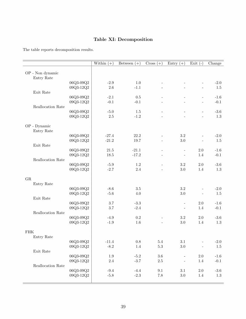
Table XI: Decomposition
The table reports decomposition results.
Within (+) Between (+) Cross (+) Entry (+) Exit (-) Change
OP - Non dynamicEntry Rate
06Q3-09Q2 -2.9 1.0 - - - -2.009Q3-12Q2 2.6 -1.1 - - - 1.5
Exit Rate06Q3-09Q2 -2.1 0.5 - - - -1.609Q3-12Q2 -0.1 -0.1 - - - -0.1
Reallocation Rate06Q3-09Q2 -5.0 1.5 - - - -3.609Q3-12Q2 2.5 -1.2 - - - 1.3
OP - DynamicEntry Rate
06Q3-09Q2 -27.4 22.2 - 3.2 - -2.009Q3-12Q2 -21.2 19.7 - 3.0 - 1.5
Exit Rate06Q3-09Q2 21.5 -21.1 - - 2.0 -1.609Q3-12Q2 18.5 -17.2 - - 1.4 -0.1
Reallocation Rate06Q3-09Q2 -5.9 1.2 - 3.2 2.0 -3.609Q3-12Q2 -2.7 2.4 - 3.0 1.4 1.3
GREntry Rate
06Q3-09Q2 -8.6 3.5 3.2 - -2.009Q3-12Q2 -5.6 4.0 3.0 - 1.5
Exit Rate06Q3-09Q2 3.7 -3.3 - 2.0 -1.609Q3-12Q2 3.7 -2.4 - 1.4 -0.1
Reallocation Rate06Q3-09Q2 -4.9 0.2 - 3.2 2.0 -3.609Q3-12Q2 -1.9 1.6 - 3.0 1.4 1.3
FHKEntry Rate
06Q3-09Q2 -11.4 0.8 5.4 3.1 - -2.009Q3-12Q2 -8.2 1.4 5.3 3.0 - 1.5
Exit Rate06Q3-09Q2 1.9 -5.2 3.6 - 2.0 -1.609Q3-12Q2 2.4 -3.7 2.5 - 1.4 -0.1
Reallocation Rate06Q3-09Q2 -9.4 -4.4 9.1 3.1 2.0 -3.609Q3-12Q2 -5.8 -2.3 7.8 3.0 1.4 1.3
39

Table XII: Summary Statistics for Aggregate Entry and Exit Rates by Types
The table reports summary statistics for within firms by types.
All (1) (2) (3) Change2007-2013 2007 2010 2013 (2)/(1)-1 (3)-(2)-1
EntryImprovement 0.038 0.042 0.032 0.041 -25% 29%Extension 0.005 0.006 0.004 0.005 -36% 42%Firm 0.003 0.004 0.003 0.003 -45% 52%
ALL 0.0045 0.052 0.038 0.050 -28% 32%
ExitImprovement 0.029 0.035 0.025 0.026 -27% 5%Extension 0.005 0.006 0.004 0.004 -35% 17%Firm 0.001 0.002 0.001 0.001 -37% 32%
ALL 0.035 0.042 0.030 0.032 -29% 7%
Table XIII: Summary Statistics for Within Entry and Exit Rates by Types
The table reports summary statistics for within firms by types.
All (1) (2) (3) Change2007-2013 2007 2010 2013 (2)/(1)-1 (3)-(2)-1
EntryImprovement 0.026 0.028 0.021 0.030 -24% 44%Extension 0.010 0.011 0.008 0.011 -28% 45%Firm 0.022 0.029 0.018 0.026 -39% 47%
ALL 0.058 0.068 0.047 0.068 -31% 45%
ExitImprovement 0.019 0.021 0.017 0.018 -22% 11%Extension 0.015 0.021 0.013 0.012 -37% -6%Firm 0.018 0.021 0.015 0.019 -30% 30%
ALL 0.052 0.063 0.045 0.050 -29% 12%
40
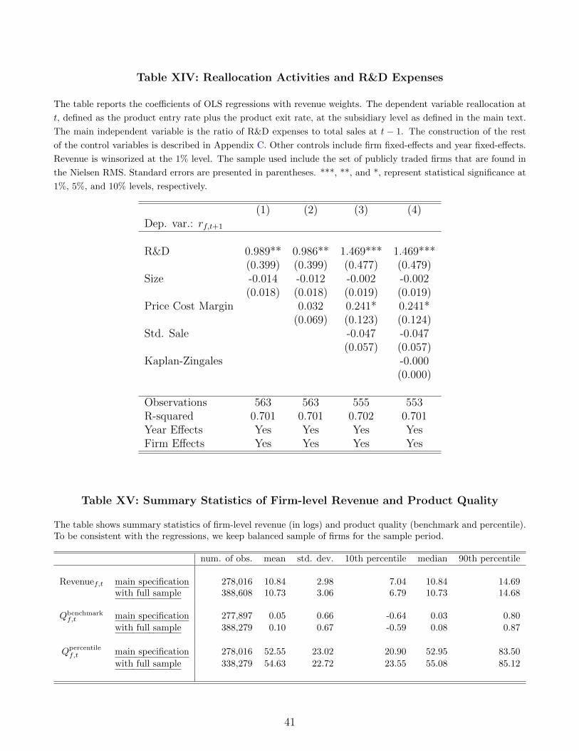
Table XIV: Reallocation Activities and R&D Expenses
The table reports the coe�cients of OLS regressions with revenue weights. The dependent variable reallocation at
t, defined as the product entry rate plus the product exit rate, at the subsidiary level as defined in the main text.
The main independent variable is the ratio of R&D expenses to total sales at t � 1. The construction of the rest
of the control variables is described in Appendix C. Other controls include firm fixed-e↵ects and year fixed-e↵ects.
Revenue is winsorized at the 1% level. The sample used include the set of publicly traded firms that are found in
the Nielsen RMS. Standard errors are presented in parentheses. ***, **, and *, represent statistical significance at
1%, 5%, and 10% levels, respectively.
(1) (2) (3) (4)Dep. var.: r
f,t+1
R&D 0.989** 0.986** 1.469*** 1.469***(0.399) (0.399) (0.477) (0.479)
Size -0.014 -0.012 -0.002 -0.002(0.018) (0.018) (0.019) (0.019)
Price Cost Margin 0.032 0.241* 0.241*(0.069) (0.123) (0.124)
Std. Sale -0.047 -0.047(0.057) (0.057)
Kaplan-Zingales -0.000(0.000)
Observations 563 563 555 553R-squared 0.701 0.701 0.702 0.701Year E↵ects Yes Yes Yes YesFirm E↵ects Yes Yes Yes Yes
Table XV: Summary Statistics of Firm-level Revenue and Product Quality
The table shows summary statistics of firm-level revenue (in logs) and product quality (benchmark and percentile).To be consistent with the regressions, we keep balanced sample of firms for the sample period.
num. of obs. mean std. dev. 10th percentile median 90th percentile
Revenuef,t main specification 278,016 10.84 2.98 7.04 10.84 14.69with full sample 388,608 10.73 3.06 6.79 10.73 14.68
Q
benchmarkf,t main specification 277,897 0.05 0.66 -0.64 0.03 0.80
with full sample 388,279 0.10 0.67 -0.59 0.08 0.87
Q
percentilef,t main specification 278,016 52.55 23.02 20.90 52.95 83.50
with full sample 338,279 54.63 22.72 23.55 55.08 85.12
41
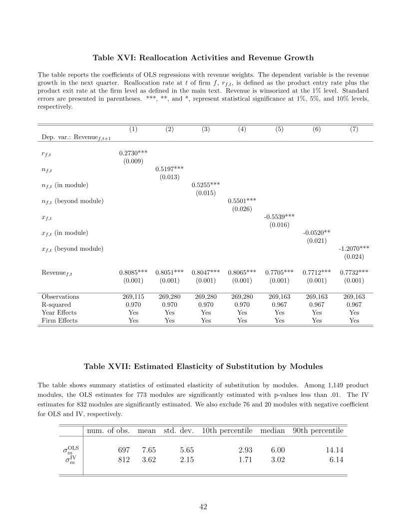
Table XVI: Reallocation Activities and Revenue Growth
The table reports the coe�cients of OLS regressions with revenue weights. The dependent variable is the revenuegrowth in the next quarter. Reallocation rate at t of firm f , rf,t, is defined as the product entry rate plus theproduct exit rate at the firm level as defined in the main text. Revenue is winsorized at the 1% level. Standarderrors are presented in parentheses. ***, **, and *, represent statistical significance at 1%, 5%, and 10% levels,respectively.
(1) (2) (3) (4) (5) (6) (7)Dep. var.: Revenuef,t+1
rf,t 0.2730***(0.009)
nf,t 0.5197***(0.013)
nf,t (in module) 0.5255***(0.015)
nf,t (beyond module) 0.5501***(0.026)
xf,t -0.5539***(0.016)
xf,t (in module) -0.0520**(0.021)
xf,t (beyond module) -1.2070***(0.024)
Revenuef,t 0.8085*** 0.8051*** 0.8047*** 0.8065*** 0.7705*** 0.7712*** 0.7732***(0.001) (0.001) (0.001) (0.001) (0.001) (0.001) (0.001)
Observations 269,115 269,280 269,280 269,280 269,163 269,163 269,163R-squared 0.970 0.970 0.970 0.970 0.967 0.967 0.967Year E↵ects Yes Yes Yes Yes Yes Yes YesFirm E↵ects Yes Yes Yes Yes Yes Yes Yes
Table XVII: Estimated Elasticity of Substitution by Modules
The table shows summary statistics of estimated elasticity of substitution by modules. Among 1,149 product
modules, the OLS estimates for 773 modules are significantly estimated with p-values less than .01. The IV
estimates for 832 modules are significantly estimated. We also exclude 76 and 20 modules with negative coe�cient
for OLS and IV, respectively.
num. of obs. mean std. dev. 10th percentile median 90th percentile
�
OLSm
697 7.65 5.65 2.93 6.00 14.14�
IVm
812 3.62 2.15 1.71 3.02 6.14
42

Table XVIII: Reallocation Activities and Benchmark Quality Improvement
The table reports the coe�cients of OLS regressions with revenue weights. The dependent variable is the benchmarkquality improvement in the next quarter. Reallocation rate at t of firm f , rf,t, is defined as the product entry rateplus the product exit rate at the firm level as defined in the main text. Revenue is winsorized at the 1% level.Standard errors are presented in parentheses. ***, **, and *, represent statistical significance at 1%, 5%, and 10%levels, respectively.
(1) (2) (3) (4) (5) (6) (7)Dep. var.: Qbenchmark
f,t+1
rf,t 0.0162***(0.003)
nf,t 0.0274***(0.004)
nf,t (in module) 0.0250***(0.005)
nf,t (beyond module) 0.0345***(0.009)
xf,t 0.0040(0.005)
xf,t (in module) -0.0183***(0.007)
xf,t (beyond module) 0.0327***(0.008)
Revenuef,t 0.0064*** 0.0061*** 0.0061*** 0.0062*** 0.0063*** 0.0062*** 0.0062***(0.000) (0.000) (0.000) (0.000) (0.000) (0.000) (0.000)
Observations 269,007 269,171 269,171 269,171 269,055 269,055 269,055R-squared 0.923 0.923 0.923 0.923 0.923 0.923 0.923Year E↵ects Yes Yes Yes Yes Yes Yes YesFirm E↵ects Yes Yes Yes Yes Yes Yes Yes
43
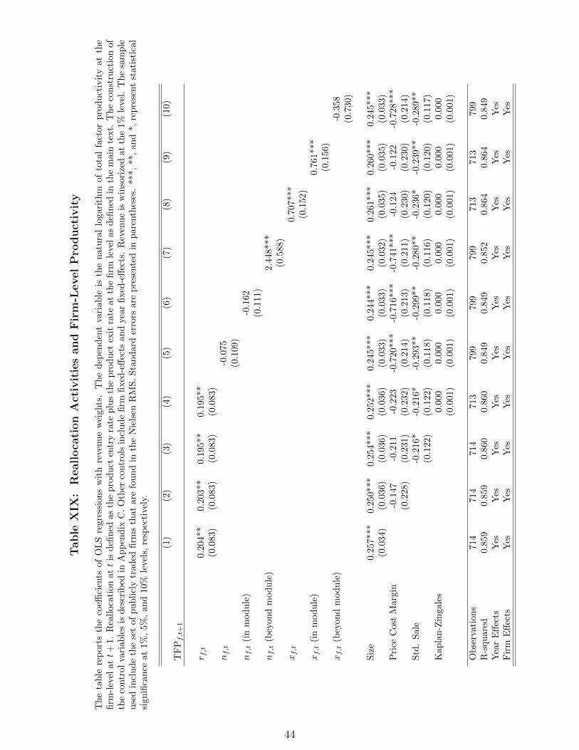
Table
XIX
:Realloca
tion
Activitiesand
Firm-L
evelPro
ductivity
Thetable
reports
thecoe�
cients
ofOLSregression
swithrevenu
eweigh
ts.Thedep
endentvariab
leis
thenaturallogarithm
oftotalfactor
productivityat
the
firm
-level
att+1.
Reallocationat
tisdefined
astheproduct
entryrate
plustheproduct
exitrate
atthefirm
levelas
defined
inthemaintext.Theconstructionof
thecontrolvariab
lesisdescribed
inAppendix
C.Other
controlsincludefirm
fixed-e↵ects
andyear
fixed-e↵ects.Revenueiswinsorizedat
the1%
level.Thesample
usedincludethesetof
publiclytrad
edfirm
sthat
arefoundin
theNielsen
RMS.Standarderrors
arepresented
inparentheses.***,
**,an
d*,
represent
statistical
sign
ificance
at1%
,5%
,an
d10%
levels,respectively.
(1)
(2)
(3)
(4)
(5)
(6)
(7)
(8)
(9)
(10)
TFPf,t+1
r
f,t
0.204**
0.203**
0.195**
0.195**
(0.083)
(0.083)
(0.083)
(0.083)
n
f,t
-0.075
(0.109)
n
f,t(inmod
ule)
-0.162
(0.111)
n
f,t(beyon
dmod
ule)
2.448***
(0.588)
x
f,t
0.707***
(0.152)
x
f,t(inmod
ule)
0.761***
(0.156)
x
f,t(beyon
dmod
ule)
-0.358
(0.730)
Size
0.257***
0.250***
0.254***
0.252***
0.245***
0.244***
0.245***
0.261***
0.260***
0.245***
(0.034)
(0.036)
(0.036)
(0.036)
(0.033)
(0.033)
(0.032)
(0.035)
(0.035)
(0.033)
Price
CostMargin
-0.147
-0.211
-0.223
-0.720***
-0.716***
-0.741***
-0.124
-0.122
-0.728***
(0.228)
(0.231)
(0.232)
(0.214)
(0.213)
(0.211)
(0.230)
(0.230)
(0.214)
Std.Sale
-0.216*
-0.216*
-0.293**
-0.299**
-0.280**
-0.236*
-0.239**
-0.289**
(0.122)
(0.122)
(0.118)
(0.118)
(0.116)
(0.120)
(0.120)
(0.117)
Kap
lan-Zingales
0.000
0.000
0.000
0.000
0.000
0.000
0.000
(0.001)
(0.001)
(0.001)
(0.001)
(0.001)
(0.001)
(0.001)
Observations
714
714
714
713
799
799
799
713
713
799
R-squ
ared
0.859
0.859
0.860
0.860
0.849
0.849
0.852
0.864
0.864
0.849
YearE↵ects
Yes
Yes
Yes
Yes
Yes
Yes
Yes
Yes
Yes
Yes
Firm
E↵ects
Yes
Yes
Yes
Yes
Yes
Yes
Yes
Yes
Yes
Yes
44
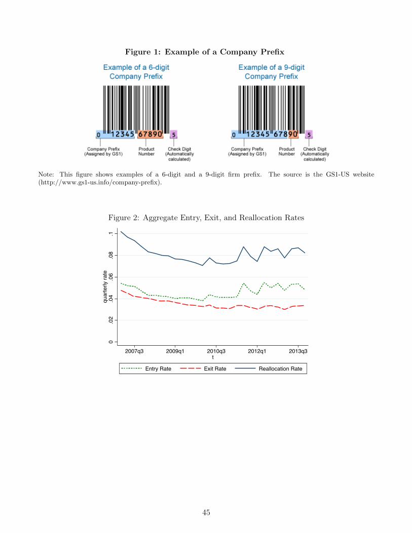
Figure 1: Example of a Company Prefix
Note: This figure shows examples of a 6-digit and a 9-digit firm prefix. The source is the GS1-US website(http://www.gs1-us.info/company-prefix).
Figure 2: Aggregate Entry, Exit, and Reallocation Rates
0.0
2.0
4.0
6.0
8.1
quar
terly
rate
2007q3 2009q1 2010q3 2012q1 2013q3t
Entry Rate Exit Rate Reallocation Rate
45

Figure 3: Within-firm Entry, Exit, and Reallocation Rates
.03
.06
.09
.12
.15
quar
terly
rate
2006q3 2008q3 2010q3 2012q3 2014q3t
Entry Rate Exit Rate Reallocation Rate
Figure 4: Aggregated and Within Reallocation
.04
.06
.08
.1.1
2.1
4qu
arte
rly ra
te
2006q3 2008q3 2010q3 2012q3 2014q3t
Average within reallocation rate (including entrant and exit firms)Average within reallocation rate among continuing firmsAggregated reallocation rate
46
A Firm Dataset
Using the product level dataset and the information on the firm, we construct a dataset with the
following information for each firm per quarter:
type of firm �it
is defined as 1 if it is the first time we see the firm (or all products of the
firm are entrants products), -1 if the last period we saw the firms was in t (or all products
of the firm are exit products), and 0 otherwise.
total number of entrant products Nit
=P
j
N
jit
number of exit products Xit
=P
j
X
jit
number of continuing products Cit
=P
j
C
jit
number of all products
– (i) Tit
computed as number of observations of products of firm i in t, defined as defined
as Nit
+ C
it
– (ii) T2it
computed as number of observations of products of firm i in t�1 plus the changes
in the number of products as defined in �T2it
, i.e. T2it�1+�T2
it
with T
i06Q1 = T2i06Q1
change in the number of products
– (i) �T
it
computed as number of products in t minus number of products in t� 1
– (ii) �T2it
computed as number of entrants in t minus number of exits in t, i.e. change
in products is defined as Nit
�X
it
entry rate n
it
= N
it
/T
it
and n2it
= N
it
/T2it
exit rate x
it
= X
it
/T
it�1 and n2it
= N
it
/T2it�1
reallocation within firm r
it
= n
it
+ x
it
and r
it
= n2it
+ x2it
total revenue of all products revit
total revenue of entrant a products revNit
total revenue of entrant b products revNa
it
total revenue of entrant c products revNb
it
total revenue of entrant d products revNc
it
total revenue of entrant d products revNd
it
47

total revenue of entrant e products revNd
it
total revenue of exit products revXit
dummy variable to indicate if is a multi-product firm (i.e. if number of products >1) multi
it
number of di↵erent modules modules
it
dummy variable to indicate if is a multi-module firm (i.e. if number of module>1)multimodules
it
number of di↵erent groups groupsit
dummy variable to indicate if is a multi-group firm (i.e. if number of group >1)multigroups
it
number of di↵erent departments departments
it
dummy variable to indicate if is a multi-department firm (i.e. if number of depart. >1)
multidepartments
it
main module (defined as the module that generates more revenue) mainmodule
it
share of revenue in main module revmainmodule
it
main group (defined as the group that generates more revenue) maingroup
it
share of revenue in main group revmaingroup
it
main department (defined as the department that generates more revenue)maindepartment
it
share of revenue in main department revmaindepartment
it
simple average quality of all products (using the variable quality0 to quality7 in the original
dataset) q0it
q1it
q2it
q3it
q4it
q5it
q6it
q7it
simple average quality of all exit products q0it
q1it
q2it
q3it
q4it
q5it
q6it
q7it
48
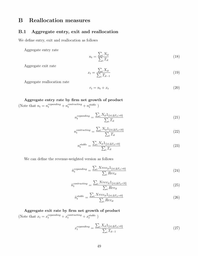
B Reallocation measures
B.1 Aggregate entry, exit and reallocation
We define entry, exit and reallocation as follows
Aggregate entry rate
n
t
=
Pi
N
itPi
T
it
(18)
Aggregate exit rate
x
t
=
Pi
X
itPi
T
it�1
(19)
Aggregate reallocation rate
r
t
= n
t
+ x
t
(20)
Aggregate entry rate by firm net growth of product
(Note that nt
= n
expanding
t
+ n
contracting
t
+ n
stable
t
)
n
expanding
t
=
Pi
N
it
1{i2�Tit>0}Pi
T
it
(21)
n
contracting
t
=
Pi
N
it
1{i2�Tit<0}Pi
T
it
(22)
n
stable
t
=
Pi
N
it
1{i2�Tit=0}Pi
T
it
(23)
We can define the revenue-weighted version as follows
n
expanding
t
=
Pi
Nrev
it
1{i2�Tit>0}Pi
Rev
it
(24)
n
contracting
t
=
Pi
Nrev
it
1{i2�Tit<0}Pi
Rev
it
(25)
n
stable
t
=
Pi
Nrev
it
1{i2�Tit=0}Pi
Rev
it
(26)
Aggregate exit rate by firm net growth of product
(Note that xt
= x
expanding
t
+ x
contracting
t
+ x
stable
t
)
x
expanding
t
=
Pi
X
it
1{i2�Tit>0}Pi
T
it�1
(27)
49
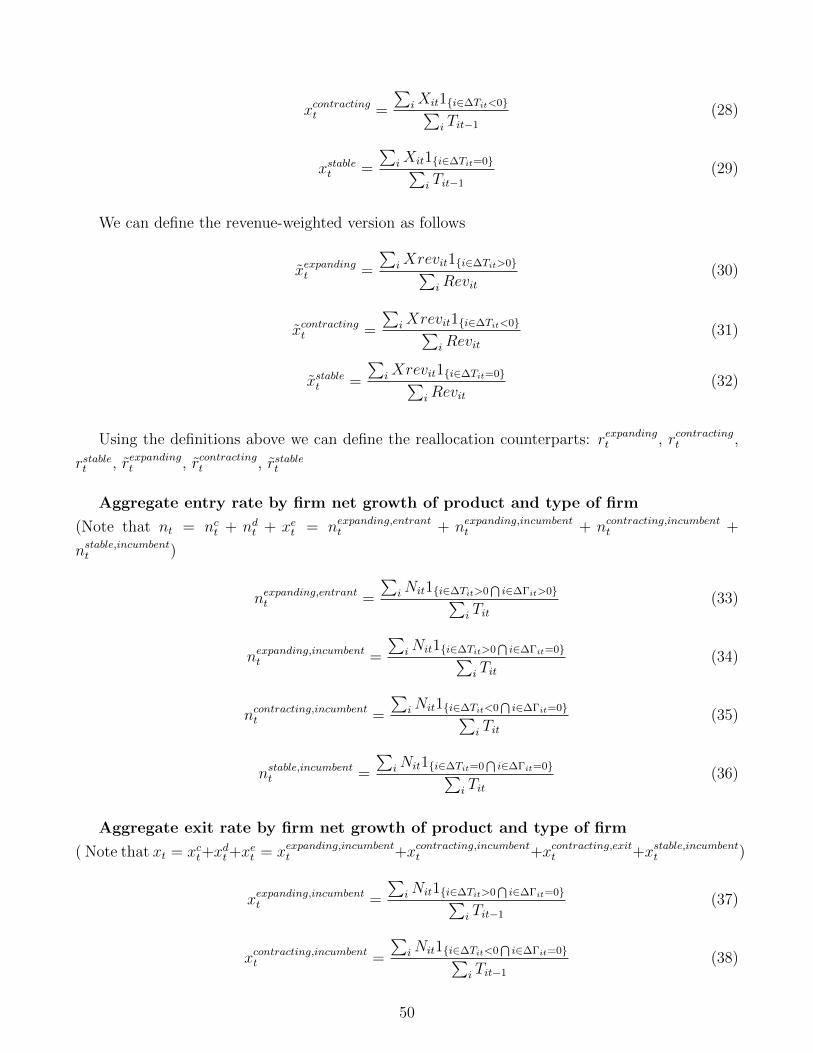
x
contracting
t
=
Pi
X
it
1{i2�Tit<0}Pi
T
it�1
(28)
x
stable
t
=
Pi
X
it
1{i2�Tit=0}Pi
T
it�1
(29)
We can define the revenue-weighted version as follows
x
expanding
t
=
Pi
Xrev
it
1{i2�Tit>0}Pi
Rev
it
(30)
x
contracting
t
=
Pi
Xrev
it
1{i2�Tit<0}Pi
Rev
it
(31)
x
stable
t
=
Pi
Xrev
it
1{i2�Tit=0}Pi
Rev
it
(32)
Using the definitions above we can define the reallocation counterparts: r
expanding
t
, rcontractingt
,
r
stable
t
, rexpandingt
, rcontractingt
, rstablet
Aggregate entry rate by firm net growth of product and type of firm
(Note that n
t
= n
c
t
+ n
d
t
+ x
e
t
= n
expanding,entrant
t
+ n
expanding,incumbent
t
+ n
contracting,incumbent
t
+
n
stable,incumbent
t
)
n
expanding,entrant
t
=
Pi
N
it
1{i2�Tit>0T
i2��it>0}Pi
T
it
(33)
n
expanding,incumbent
t
=
Pi
N
it
1{i2�Tit>0T
i2��it=0}Pi
T
it
(34)
n
contracting,incumbent
t
=
Pi
N
it
1{i2�Tit<0T
i2��it=0}Pi
T
it
(35)
n
stable,incumbent
t
=
Pi
N
it
1{i2�Tit=0T
i2��it=0}Pi
T
it
(36)
Aggregate exit rate by firm net growth of product and type of firm
( Note that xt
= x
c
t
+x
d
t
+x
e
t
= x
expanding,incumbent
t
+x
contracting,incumbent
t
+x
contracting,exit
t
+x
stable,incumbent
t
)
x
expanding,incumbent
t
=
Pi
N
it
1{i2�Tit>0T
i2��it=0}Pi
T
it�1
(37)
x
contracting,incumbent
t
=
Pi
N
it
1{i2�Tit<0T
i2��it=0}Pi
T
it�1
(38)
50
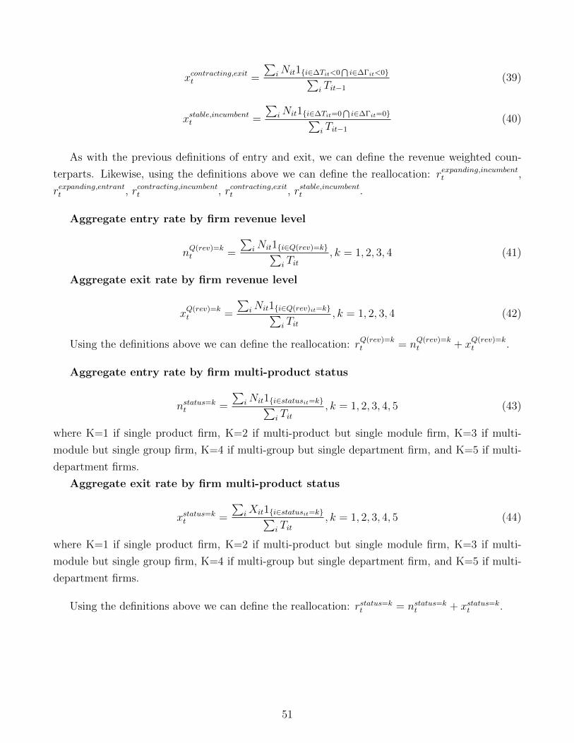
x
contracting,exit
t
=
Pi
N
it
1{i2�Tit<0T
i2��it<0}Pi
T
it�1
(39)
x
stable,incumbent
t
=
Pi
N
it
1{i2�Tit=0T
i2��it=0}Pi
T
it�1
(40)
As with the previous definitions of entry and exit, we can define the revenue weighted coun-
terparts. Likewise, using the definitions above we can define the reallocation: r
expanding,incumbent
t
,
r
expanding,entrant
t
, rcontracting,incumbent
t
, rcontracting,exitt
, rstable,incumbent
t
.
Aggregate entry rate by firm revenue level
n
Q(rev)=k
t
=
Pi
N
it
1{i2Q(rev)=k}Pi
T
it
, k = 1, 2, 3, 4 (41)
Aggregate exit rate by firm revenue level
x
Q(rev)=k
t
=
Pi
N
it
1{i2Q(rev)it=k}Pi
T
it
, k = 1, 2, 3, 4 (42)
Using the definitions above we can define the reallocation: rQ(rev)=k
t
= n
Q(rev)=k
t
+ x
Q(rev)=k
t
.
Aggregate entry rate by firm multi-product status
n
status=k
t
=
Pi
N
it
1{i2statusit=k}Pi
T
it
, k = 1, 2, 3, 4, 5 (43)
where K=1 if single product firm, K=2 if multi-product but single module firm, K=3 if multi-
module but single group firm, K=4 if multi-group but single department firm, and K=5 if multi-
department firms.
Aggregate exit rate by firm multi-product status
x
status=k
t
=
Pi
X
it
1{i2statusit=k}Pi
T
it
, k = 1, 2, 3, 4, 5 (44)
where K=1 if single product firm, K=2 if multi-product but single module firm, K=3 if multi-
module but single group firm, K=4 if multi-group but single department firm, and K=5 if multi-
department firms.
Using the definitions above we can define the reallocation: rstatus=k
t
= n
status=k
t
+ x
status=k
t
.
51
C Construction of Variables: Compustat
We use the Compustat fundamental annual data from 2006 to 2014. Our sample consists of all
firms that have positive data on sales that do not belong to the finance or real estate sectors
(SIC classification between 6010 and 6800). To compute total factor productivity (TFP) we
follow the methodology of Imrohoroglu and Tuzel (2014). TFP is estimated using the semi-
parametric method by Olley and Pakes (1996). We supplement the Compustat data with output
and investment deflators from the Bureau of Economic Analysis and wage data from the Social
Security Administration.
We compute R&D as the ratio of research and development expenses (Compustat item XRD)
to net sales (Compustat item SALE). We winsorize the variable at the 1% level and use the one-
year lagged value of in our regressions. Size is the natural logarithm of total sales. Given that
total sta↵ expenses (Compustat item XLR) is mostly missing in our data, we define labor share as
the ratio of the number of employees (Compustat item EMP) times the national wage (obtained
from the Social Security Administration) over net sales. Std Sale is defined as the volatility of
annual growth of sales on a quarterly basis winsorized at the 1% level.
We follow Gorodnichenko and Weber (2016) to construct the rest of our control variables.
Specifically, Price to cost margin (PCM) is the ratio of net sales minus costs of goods sold (Com-
pustat item COGS) to net sales. Rating (Rat) is the S&P domestic long term issuer credit rating
(Compustat item SPLTICRM) where the highest rating category, AAA, is assigned a value of 4.33,
decreasing by 1/8 with every rating notch. We use the one-year lagged value of the mean ratings
within the year. In order to control for financial constraints, we include the Kaplan-Zingales index
(KZ, Kaplan and Zingales (1997)) defined as follows:
KZ
i,t
= 1.002CF
i,t
AT
i,t1
� 39.368Div
i,t
AT
i,t�1
� 1.315C
i,t
AT
i,t1
+ 3.139Levi,t
+ 0.283Qi,t
(45)
where cash flow (CF) is the sum of income before extraordinary items (Compustat item IB) and
depreciation and amortization, dividends (Div) are measured as common and preferred dividends
(Compustat items DVC and DVP), C is cash and short term investments (Compustat item CHE),
leverage (Lev) is the ratio of long term debt and debt in current liabilities (Compustat items DLTT
and DLC) to stockholders equity (Compustat item SEQ), and Q is the market value of equity from
CRSP as of fiscal year end minus the bookvalue of equity and deferred taxes (Compustat items
CEQ and TXDB) to total assets. The first three variables are normalized by lagged total assets.
We winsorize all variables at the 1% level before calculating the index and use one-year lagged
values of the index in our regressions.
52
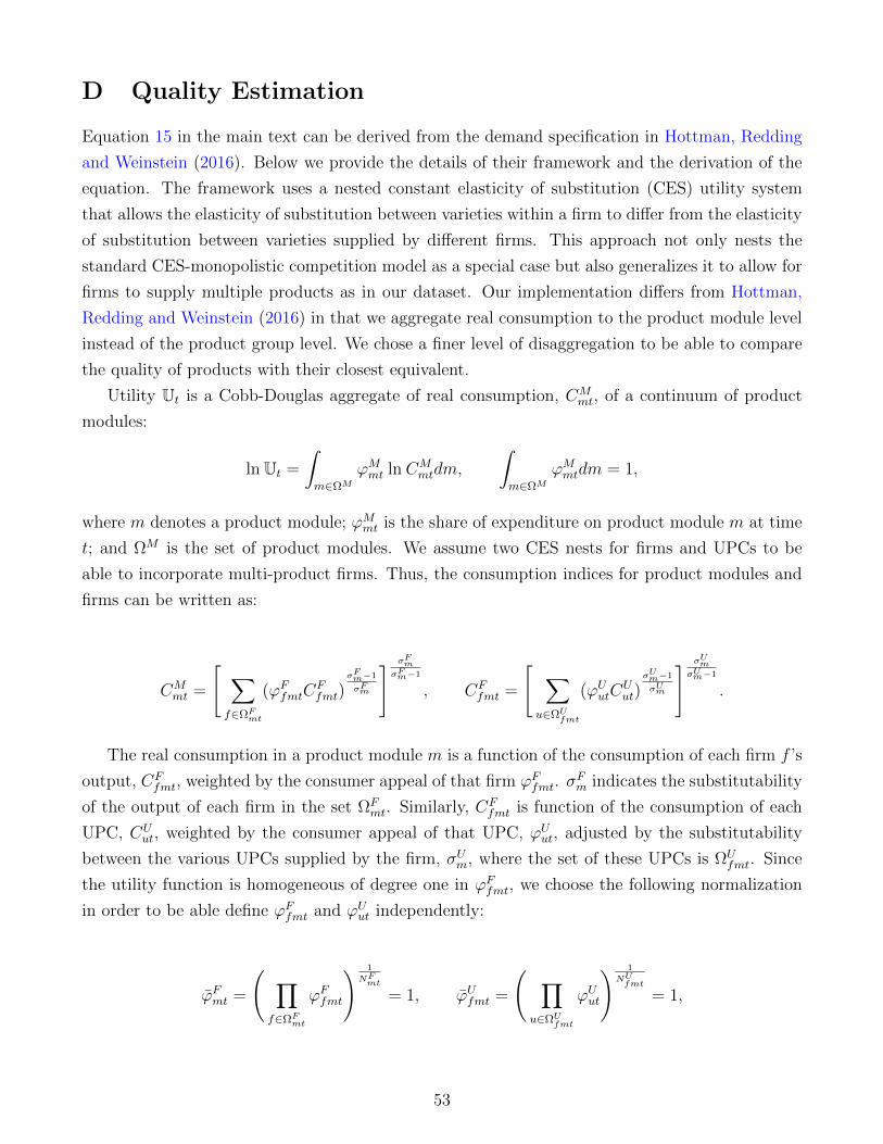
D Quality Estimation
Equation 15 in the main text can be derived from the demand specification in Hottman, Redding
and Weinstein (2016). Below we provide the details of their framework and the derivation of the
equation. The framework uses a nested constant elasticity of substitution (CES) utility system
that allows the elasticity of substitution between varieties within a firm to di↵er from the elasticity
of substitution between varieties supplied by di↵erent firms. This approach not only nests the
standard CES-monopolistic competition model as a special case but also generalizes it to allow for
firms to supply multiple products as in our dataset. Our implementation di↵ers from Hottman,
Redding and Weinstein (2016) in that we aggregate real consumption to the product module level
instead of the product group level. We chose a finer level of disaggregation to be able to compare
the quality of products with their closest equivalent.
Utility Ut
is a Cobb-Douglas aggregate of real consumption, CM
mt
, of a continuum of product
modules:
ln Ut
=
Z
m2⌦M
'
M
mt
ln C
M
mt
dm,
Z
m2⌦M
'
M
mt
dm = 1,
where m denotes a product module; 'M
mt
is the share of expenditure on product module m at time
t; and ⌦M is the set of product modules. We assume two CES nests for firms and UPCs to be
able to incorporate multi-product firms. Thus, the consumption indices for product modules and
firms can be written as:
C
M
mt
=
"X
f2⌦Fmt
('F
fmt
C
F
fmt
)�Fm�1
�Fm
# �Fm
�Fm�1
, C
F
fmt
=
"X
u2⌦Ufmt
('U
ut
C
U
ut
)�Um�1
�Um
# �Um
�Um�1
.
The real consumption in a product module m is a function of the consumption of each firm f ’s
output, CF
fmt
, weighted by the consumer appeal of that firm '
F
fmt
. �F
m
indicates the substitutability
of the output of each firm in the set ⌦F
mt
. Similarly, CF
fmt
is function of the consumption of each
UPC, CU
ut
, weighted by the consumer appeal of that UPC, 'U
ut
, adjusted by the substitutability
between the various UPCs supplied by the firm, �U
m
, where the set of these UPCs is ⌦U
fmt
. Since
the utility function is homogeneous of degree one in '
F
fmt
, we choose the following normalization
in order to be able define '
F
fmt
and '
U
ut
independently:
'
F
mt
=
Y
f2⌦Fmt
'
F
fmt
! 1
NFmt
= 1, '
U
fmt
=
Y
u2⌦Ufmt
'
U
ut
! 1
NUfmt
= 1,
53

where N
F
mt
is the number of firms in module m at time t and N
U
fmt
is the number of UPCs
supplied by firm f within module m at time t. The product module price index and the firm price
index are:
P
G
mt
=
"X
f2⌦Fmt
P
F
fmt
'
F
fmt
!1��
F# 11��F
, P
F
fmt
=
"X
u2⌦Ufmt
P
U
ut
'
U
ut
!1��
U# 11��U
.
Under this specification, the demand for the output of UPC u supplied by firm f within product
module m is therefore:
C
U
ut
= ('F
fmt
)�F�1(P F
fmt
)�U��
FE
G
mt
(PM
mt
)�F�1(PU
ut
)��
U('U
ut
)�U�1
We model 'U
ut
as the product of a fixed component '
U
u
, which captures persistent di↵erences
across products in terms of perceived quality, and ⌘
U
ut
which measures idiosyncratic variation in the
preferences for each UPC u. Taking logs and substituting with �
fmt
the firm-specific components
(in logs), we can write:
ln(CU
ut
) = �
fmt
� �
U
ln(PU
ut
) + (�U � 1)'U
u
+ (�U � 1)⌘Uut
(46)
Equation 46 suggests that product quality '
U
u
can be estimated from the data in a regression
of quantity demanded on price and firm-module-time fixed e↵ects. Nonetheless, it is well known
that estimating equation 46 using OLS will deliver biased estimates for �
U , the module-specific
elasticity of substitution, and for '
U
u
, the UPC specific quality. In order to solve the standard
simultaneity concern, we use the estimation procedure described in Fally and Faber (2017), which
relies on instrumenting for local consumer price changes using regional variation. Given that each
UPC u belongs to a single firm f , product module m, and is sold in city c, we can rewrite equation
46 as:
ln(Cufmct
) = �
fmct
� �ln(Pufmct
) + (� � 1)'u
+ ✏
ufmct
(47)
which is the analog of equation 15 in the main text.
54

Appendix Tables and Figures (FOR ONLINE PUBLICA-
TION)
Table A.I: Summary Statistics of Products (with Full Sample)
The table shows summary statistics of products.
06Q3 2007 2010 2013
Number of products 608368 605139 610356 602407
By status (share of products)Entrants 0.039 0.052 0.032 0.042Exits 0.038 0.035 0.035 0.046
By diversification (average)Per module 565 587 575 593Per group 5300 5506 5397 5559Per department 60422 62769 61526 63376
By Revenue (share of products)[0,104[ 0.676 0.698 0.695 0.693[104,105[ 0.187 0.192 0.191 0.191[105,106[ 0.096 0.095 0.098 0.100>=106 0.041 0.015 0.016 0.016
55
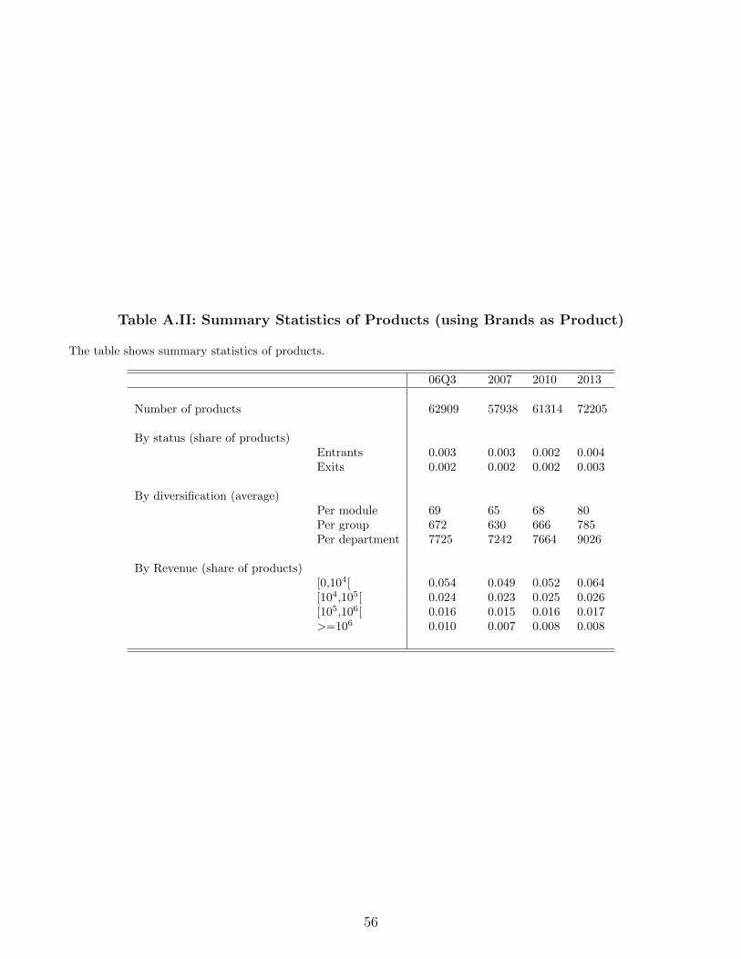
Table A.II: Summary Statistics of Products (using Brands as Product)
The table shows summary statistics of products.
06Q3 2007 2010 2013
Number of products 62909 57938 61314 72205
By status (share of products)Entrants 0.003 0.003 0.002 0.004Exits 0.002 0.002 0.002 0.003
By diversification (average)Per module 69 65 68 80Per group 672 630 666 785Per department 7725 7242 7664 9026
By Revenue (share of products)[0,104[ 0.054 0.049 0.052 0.064[104,105[ 0.024 0.023 0.025 0.026[105,106[ 0.016 0.015 0.016 0.017>=106 0.010 0.007 0.008 0.008
56
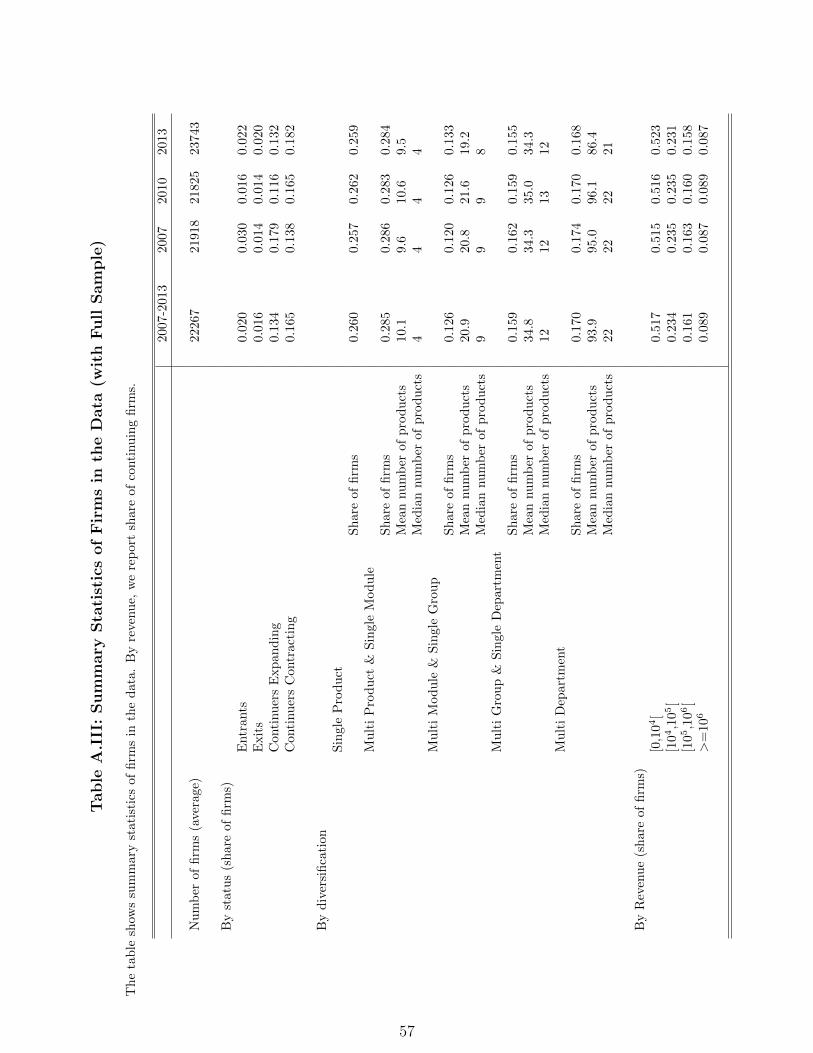
Table
A.III:Summary
StatisticsofFirmsin
theData
(with
Full
Sample)
Thetable
show
ssummarystatistics
offirm
sin
thedata.
Byrevenu
e,wereportshareof
continuingfirm
s.
2007-2013
2007
2010
2013
Number
offirm
s(average)
22267
21918
21825
23743
Bystatus(shareof
firm
s)Entrants
0.020
0.030
0.016
0.022
Exits
0.016
0.014
0.014
0.020
Con
tinu
ersExp
anding
0.134
0.179
0.116
0.132
Con
tinu
ersCon
tracting
0.165
0.138
0.165
0.182
Bydiversification
SingleProduct
Shareof
firm
s0.260
0.257
0.262
0.259
MultiProduct
&SingleMod
ule
Shareof
firm
s0.285
0.286
0.283
0.284
Meannu
mber
ofproducts
10.1
9.6
10.6
9.5
Mediannu
mber
ofproducts
44
44
MultiMod
ule
&SingleGroup
Shareof
firm
s0.126
0.120
0.126
0.133
Meannu
mber
ofproducts
20.9
20.8
21.6
19.2
Mediannu
mber
ofproducts
99
98
MultiGroup&
SingleDepartm
ent
Shareof
firm
s0.159
0.162
0.159
0.155
Meannu
mber
ofproducts
34.8
34.3
35.0
34.3
Mediannu
mber
ofproducts
1212
1312
MultiDepartm
ent
Shareof
firm
s0.170
0.174
0.170
0.168
Meannu
mber
ofproducts
93.9
95.0
96.1
86.4
Mediannu
mber
ofproducts
2222
2221
ByRevenue(shareof
firm
s)[0,104[
0.517
0.515
0.516
0.523
[104,105[
0.234
0.235
0.235
0.231
[105,106[
0.161
0.163
0.160
0.158
>=10
60.089
0.087
0.089
0.087
57

Table
A.IV:Summary
StatisticsofFirmsin
theData
(usingBra
ndsasPro
duct)
Thetable
show
ssummarystatistics
offirm
sin
thedata.
Byrevenu
e,wereportshareof
continuingfirm
s.
2007-2013
2007
2010
2013
Number
offirm
s(average)
13431
13094
13016
14810
Bystatus(shareof
firm
s)Entrants
0.021
0.025
0.017
0.026
Exits
0.016
0.020
0.013
0.016
Con
tinu
ersExp
anding
0.057
0.061
0.051
0.068
Con
tinu
ersCon
tracting
0.045
0.051
0.041
0.044
Bydiversification
SingleProduct
Shareof
firm
s0.462
0.476
0.458
0.450
MultiProduct
&SingleMod
ule
Shareof
firm
s0.062
0.060
0.063
0.062
Meannu
mber
ofproducts
2.6
2.6
2.6
2.7
Mediannu
mber
ofproducts
22
22
MultiMod
ule
&SingleGroup
Shareof
firm
s0.120
0.114
0.122
0.124
Meannu
mber
ofproducts
3.8
3.6
3.8
3.8
Mediannu
mber
ofproducts
33
33
MultiGroup&
SingleDepartm
ent
Shareof
firm
s0.197
0.195
0.198
0.199
Meannu
mber
ofproducts
6.8
6.5
6.9
7.0
Mediannu
mber
ofproducts
44
44
MultiDepartm
ent
Shareof
firm
s0.159
0.155
0.159
0.165
Meannu
mber
ofproducts
14.3
13.8
14.3
14.5
Mediannu
mber
ofproducts
66
66
ByRevenue(shareof
firm
s)[0,104[
0.422
0.431
0.411
0.440
[104,105[
0.272
0.266
0.276
0.267
[105,106[
0.197
0.198
0.202
0.188
>=10
60.109
0.105
0.112
0.106
58
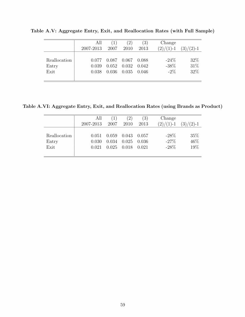
Table A.V: Aggregate Entry, Exit, and Reallocation Rates (with Full Sample)
All (1) (2) (3) Change2007-2013 2007 2010 2013 (2)/(1)-1 (3)/(2)-1
Reallocation 0.077 0.087 0.067 0.088 -24% 32%Entry 0.039 0.052 0.032 0.042 -38% 31%Exit 0.038 0.036 0.035 0.046 -2% 32%
Table A.VI: Aggregate Entry, Exit, and Reallocation Rates (using Brands as Product)
All (1) (2) (3) Change2007-2013 2007 2010 2013 (2)/(1)-1 (3)/(2)-1
Reallocation 0.051 0.059 0.043 0.057 -28% 35%Entry 0.030 0.034 0.025 0.036 -27% 46%Exit 0.021 0.025 0.018 0.021 -28% 19%
59
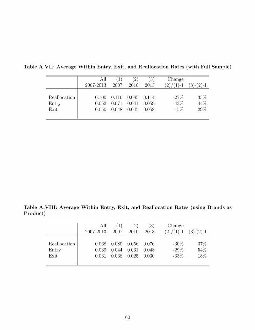
Table A.VII: Average Within Entry, Exit, and Reallocation Rates (with Full Sample)
All (1) (2) (3) Change2007-2013 2007 2010 2013 (2)/(1)-1 (3)-(2)-1
Reallocation 0.100 0.116 0.085 0.114 -27% 35%Entry 0.052 0.071 0.041 0.059 -43% 44%Exit 0.050 0.048 0.045 0.058 -5% 29%
Table A.VIII: Average Within Entry, Exit, and Reallocation Rates (using Brands asProduct)
All (1) (2) (3) Change2007-2013 2007 2010 2013 (2)/(1)-1 (3)-(2)-1
Reallocation 0.068 0.080 0.056 0.076 -30% 37%Entry 0.039 0.044 0.031 0.048 -29% 54%Exit 0.031 0.038 0.025 0.030 -33% 18%
60
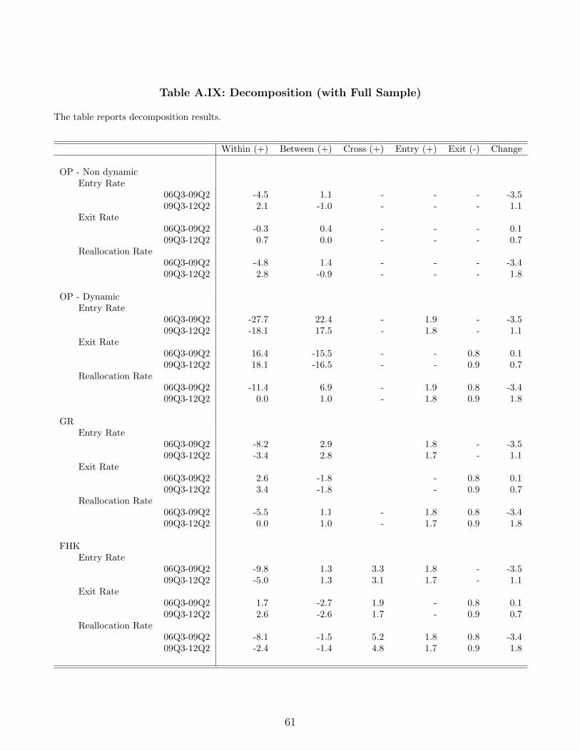
Table A.IX: Decomposition (with Full Sample)
The table reports decomposition results.
Within (+) Between (+) Cross (+) Entry (+) Exit (-) Change
OP - Non dynamicEntry Rate
06Q3-09Q2 -4.5 1.1 - - - -3.509Q3-12Q2 2.1 -1.0 - - - 1.1
Exit Rate06Q3-09Q2 -0.3 0.4 - - - 0.109Q3-12Q2 0.7 0.0 - - - 0.7
Reallocation Rate06Q3-09Q2 -4.8 1.4 - - - -3.409Q3-12Q2 2.8 -0.9 - - - 1.8
OP - DynamicEntry Rate
06Q3-09Q2 -27.7 22.4 - 1.9 - -3.509Q3-12Q2 -18.1 17.5 - 1.8 - 1.1
Exit Rate06Q3-09Q2 16.4 -15.5 - - 0.8 0.109Q3-12Q2 18.1 -16.5 - - 0.9 0.7
Reallocation Rate06Q3-09Q2 -11.4 6.9 - 1.9 0.8 -3.409Q3-12Q2 0.0 1.0 - 1.8 0.9 1.8
GREntry Rate
06Q3-09Q2 -8.2 2.9 1.8 - -3.509Q3-12Q2 -3.4 2.8 1.7 - 1.1
Exit Rate06Q3-09Q2 2.6 -1.8 - 0.8 0.109Q3-12Q2 3.4 -1.8 - 0.9 0.7
Reallocation Rate06Q3-09Q2 -5.5 1.1 - 1.8 0.8 -3.409Q3-12Q2 0.0 1.0 - 1.7 0.9 1.8
FHKEntry Rate
06Q3-09Q2 -9.8 1.3 3.3 1.8 - -3.509Q3-12Q2 -5.0 1.3 3.1 1.7 - 1.1
Exit Rate06Q3-09Q2 1.7 -2.7 1.9 - 0.8 0.109Q3-12Q2 2.6 -2.6 1.7 - 0.9 0.7
Reallocation Rate06Q3-09Q2 -8.1 -1.5 5.2 1.8 0.8 -3.409Q3-12Q2 -2.4 -1.4 4.8 1.7 0.9 1.8
61
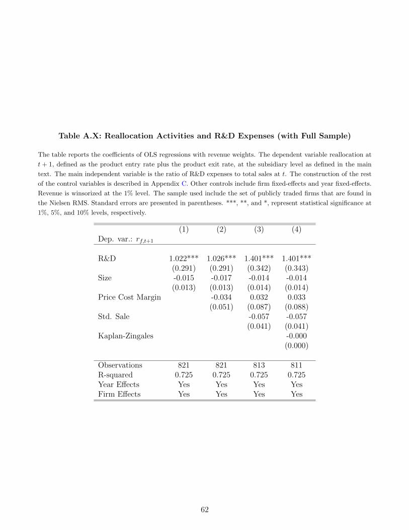
Table A.X: Reallocation Activities and R&D Expenses (with Full Sample)
The table reports the coe�cients of OLS regressions with revenue weights. The dependent variable reallocation at
t + 1, defined as the product entry rate plus the product exit rate, at the subsidiary level as defined in the main
text. The main independent variable is the ratio of R&D expenses to total sales at t. The construction of the rest
of the control variables is described in Appendix C. Other controls include firm fixed-e↵ects and year fixed-e↵ects.
Revenue is winsorized at the 1% level. The sample used include the set of publicly traded firms that are found in
the Nielsen RMS. Standard errors are presented in parentheses. ***, **, and *, represent statistical significance at
1%, 5%, and 10% levels, respectively.
(1) (2) (3) (4)Dep. var.: r
f,t+1
R&D 1.022*** 1.026*** 1.401*** 1.401***(0.291) (0.291) (0.342) (0.343)
Size -0.015 -0.017 -0.014 -0.014(0.013) (0.013) (0.014) (0.014)
Price Cost Margin -0.034 0.032 0.033(0.051) (0.087) (0.088)
Std. Sale -0.057 -0.057(0.041) (0.041)
Kaplan-Zingales -0.000(0.000)
Observations 821 821 813 811R-squared 0.725 0.725 0.725 0.725Year E↵ects Yes Yes Yes YesFirm E↵ects Yes Yes Yes Yes
62
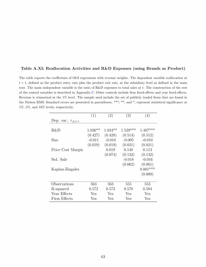
Table A.XI: Reallocation Activities and R&D Expenses (using Brands as Product)
The table reports the coe�cients of OLS regressions with revenue weights. The dependent variable reallocation at
t + 1, defined as the product entry rate plus the product exit rate, at the subsidiary level as defined in the main
text. The main independent variable is the ratio of R&D expenses to total sales at t. The construction of the rest
of the control variables is described in Appendix C. Other controls include firm fixed-e↵ects and year fixed-e↵ects.
Revenue is winsorized at the 1% level. The sample used include the set of publicly traded firms that are found in
the Nielsen RMS. Standard errors are presented in parentheses. ***, **, and *, represent statistical significance at
1%, 5%, and 10% levels, respectively.
(1) (2) (3) (4)Dep. var.: r
f,t+1
R&D 1.026** 1.024** 1.529*** 1.487***(0.427) (0.428) (0.514) (0.512)
Size -0.011 -0.010 -0.005 -0.010(0.019) (0.019) (0.021) (0.021)
Price Cost Margin 0.019 0.148 0.113(0.074) (0.132) (0.132)
Std. Sale -0.018 -0.016(0.062) (0.061)
Kaplan-Zingales 0.001***(0.000)
Observations 563 563 555 553R-squared 0.572 0.572 0.578 0.584Year E↵ects Yes Yes Yes YesFirm E↵ects Yes Yes Yes Yes
63

Table A.XII: Reallocation Activities and Revenue Growth (with Full Sample)
The table reports the coe�cients of OLS regressions with revenue weights. The dependent variable is the revenuegrowth in the next quarter. Reallocation rate at t of firm f , rf,t, is defined as the product entry rate plus theproduct exit rate at the firm level as defined in the main text. Revenue is winsorized at the 1% level. Standarderrors are presented in parentheses. ***, **, and *, represent statistical significance at 1%, 5%, and 10% levels,respectively.
(1) (2) (3) (4) (5) (6) (7)Dep. var.: Revenuef,t+1
rf,t 0.0774***(0.012)
nf,t 0.7734***(0.016)
nf,t (in module) 0.8595***(0.019)
nf,t (beyond module) 0.6970***(0.037)
xf,t -1.2398***(0.020)
xf,t (in module) -0.2674***(0.026)
xf,t (beyond module) -2.8147***(0.033)
Revenuef,t 0.6896*** 0.6869*** 0.6862*** 0.6892*** 0.6766*** 0.6773*** 0.6847***(0.001) (0.001) (0.001) (0.001) (0.001) (0.001) (0.001)
Observations 376,243 376,433 376,433 376,433 376,274 376,274 376,274R-squared 0.944 0.944 0.944 0.944 0.943 0.943 0.944Year E↵ects Yes Yes Yes Yes Yes Yes YesFirm E↵ects Yes Yes Yes Yes Yes Yes Yes
64
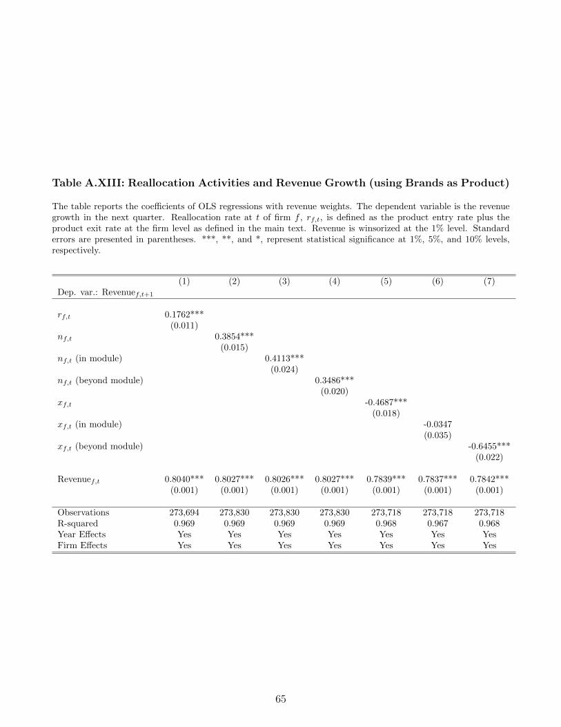
Table A.XIII: Reallocation Activities and Revenue Growth (using Brands as Product)
The table reports the coe�cients of OLS regressions with revenue weights. The dependent variable is the revenuegrowth in the next quarter. Reallocation rate at t of firm f , rf,t, is defined as the product entry rate plus theproduct exit rate at the firm level as defined in the main text. Revenue is winsorized at the 1% level. Standarderrors are presented in parentheses. ***, **, and *, represent statistical significance at 1%, 5%, and 10% levels,respectively.
(1) (2) (3) (4) (5) (6) (7)Dep. var.: Revenuef,t+1
rf,t 0.1762***(0.011)
nf,t 0.3854***(0.015)
nf,t (in module) 0.4113***(0.024)
nf,t (beyond module) 0.3486***(0.020)
xf,t -0.4687***(0.018)
xf,t (in module) -0.0347(0.035)
xf,t (beyond module) -0.6455***(0.022)
Revenuef,t 0.8040*** 0.8027*** 0.8026*** 0.8027*** 0.7839*** 0.7837*** 0.7842***(0.001) (0.001) (0.001) (0.001) (0.001) (0.001) (0.001)
Observations 273,694 273,830 273,830 273,830 273,718 273,718 273,718R-squared 0.969 0.969 0.969 0.969 0.968 0.967 0.968Year E↵ects Yes Yes Yes Yes Yes Yes YesFirm E↵ects Yes Yes Yes Yes Yes Yes Yes
65
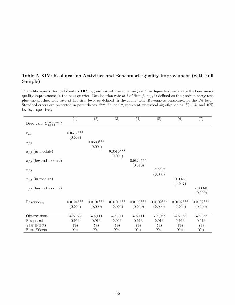
Table A.XIV: Reallocation Activities and Benchmark Quality Improvement (with FullSample)
The table reports the coe�cients of OLS regressions with revenue weights. The dependent variable is the benchmarkquality improvement in the next quarter. Reallocation rate at t of firm f , rf,t, is defined as the product entry rateplus the product exit rate at the firm level as defined in the main text. Revenue is winsorized at the 1% level.Standard errors are presented in parentheses. ***, **, and *, represent statistical significance at 1%, 5%, and 10%levels, respectively.
(1) (2) (3) (4) (5) (6) (7)Dep. var.: Qbenchmark
f,t+1
rf,t 0.0312***(0.003)
nf,t 0.0580***(0.004)
nf,t (in module) 0.0510***(0.005)
nf,t (beyond module) 0.0823***(0.010)
xf,t -0.0017(0.005)
xf,t (in module) 0.0022(0.007)
xf,t (beyond module) -0.0080(0.009)
Revenuef,t 0.0104*** 0.0101*** 0.0101*** 0.0103*** 0.0102*** 0.0102*** 0.0102***(0.000) (0.000) (0.000) (0.000) (0.000) (0.000) (0.000)
Observations 375,922 376,111 376,111 376,111 375,953 375,953 375,953R-squared 0.913 0.913 0.913 0.913 0.913 0.913 0.913Year E↵ects Yes Yes Yes Yes Yes Yes YesFirm E↵ects Yes Yes Yes Yes Yes Yes Yes
66

Table A.XV: Reallocation Activities and Benchmark Quality Improvement (usingBrands as Product)
The table reports the coe�cients of OLS regressions with revenue weights. The dependent variable is the benchmarkquality improvement in the next quarter. Reallocation rate at t of firm f , rf,t, is defined as the product entry rateplus the product exit rate at the firm level as defined in the main text. Revenue is winsorized at the 1% level.Standard errors are presented in parentheses. ***, **, and *, represent statistical significance at 1%, 5%, and 10%levels, respectively.
(1) (2) (3) (4) (5) (6) (7)Dep. var.: Qbenchmark
f,t+1
rf,t 0.0213***(0.004)
nf,t 0.0440***(0.005)
nf,t (in module) 0.0341***(0.009)
nf,t (beyond module) 0.0546***(0.007)
xf,t -0.0088(0.006)
xf,t (in module) -0.0111(0.012)
xf,t (beyond module) -0.0079(0.008)
Revenuef,t 0.0036*** 0.0035*** 0.0035*** 0.0035*** 0.0035*** 0.0035*** 0.0035***(0.000) (0.000) (0.000) (0.000) (0.000) (0.000) (0.000)
Observations 273,609 273,745 273,745 273,745 273,633 273,633 273,633R-squared 0.916 0.916 0.916 0.916 0.916 0.916 0.916Year E↵ects Yes Yes Yes Yes Yes Yes YesFirm E↵ects Yes Yes Yes Yes Yes Yes Yes
67

Table
A.X
VI:
Realloca
tion
Activitiesand
Firm-L
evelPro
ductivity(w
ith
Full
Sample)
Thetable
reports
thecoe�
cients
ofOLSregression
swithrevenu
eweigh
ts.Thedep
endentvariab
leis
thenaturallogarithm
oftotalfactor
productivityat
the
firm
-level
att+1.
Reallocationat
tisdefined
astheproduct
entryrate
plustheproduct
exitrate
atthefirm
levelas
defined
inthemaintext.Theconstructionof
thecontrolvariab
lesisdescribed
inAppendix
C.Other
controlsincludefirm
fixed-e↵ects
andyear
fixed-e↵ects.Revenueiswinsorizedat
the1%
level.Thesample
usedincludethesetof
publiclytrad
edfirm
sthat
arefoundin
theNielsen
RMS.Standarderrors
arepresented
inparentheses.***,
**,an
d*,
represent
statistical
sign
ificance
at1%
,5%
,an
d10%
levels,respectively.
(1)
(2)
(3)
(4)
(5)
(6)
(7)
(8)
(9)
(10)
TFPf,t+1
r
f,t
0.258***
0.256***
0.243***
0.242***
(0.087)
(0.087)
(0.087)
(0.087)
n
f,t
-0.028
(0.109)
n
f,t(inmod
ule)
-0.128
(0.111)
n
f,t(beyon
dmod
ule)
2.982***
(0.602)
x
f,t
0.647***
(0.147)
x
f,t(inmod
ule)
0.675***
(0.149)
x
f,t(beyon
dmod
ule)
0.058
(0.726)
Size
0.231***
0.226***
0.230***
0.228***
0.236***
0.235***
0.238***
0.230***
0.229***
0.237***
(0.029)
(0.030)
(0.030)
(0.030)
(0.027)
(0.027)
(0.027)
(0.030)
(0.030)
(0.027)
Price
CostMargin
-0.118
-0.169
-0.182
-0.668***
-0.659***
-0.670***
-0.066
-0.061
-0.670***
(0.205)
(0.205)
(0.206)
(0.190)
(0.190)
(0.188)
(0.207)
(0.207)
(0.190)
Std.Sale
-0.240**
-0.239**
-0.323***
-0.332***
-0.319***
-0.266**
-0.262
**-0.321***
(0.105)
(0.105)
(0.101)
(0.101)
(0.099)
(0.104)
(0.104)
(0.100)
Kap
lan-Zingales
0.000
0.000
0.000
0.000
0.000
0.000
0.000
(0.001)
(0.001)
(0.001)
(0.001)
(0.001)
(0.001)
(0.001)
Observations
1,024
1,024
1,024
1,023
1,147
1,147
1,147
1,023
1,023
1,147
R-squ
ared
0.843
0.843
0.844
0.845
0.834
0.834
0.838
0.847
0.847
0.834
YearE↵ects
Yes
Yes
Yes
Yes
Yes
Yes
Yes
Yes
Yes
Yes
Firm
E↵ects
Yes
Yes
Yes
Yes
Yes
Yes
Yes
Yes
Yes
Yes
68

Table
A.X
VII:
Realloca
tion
Activitiesand
Firm-L
evelPro
ductivity(u
singBra
ndsasPro
duct)
Thetable
reports
thecoe�
cients
ofOLSregression
swithrevenu
eweigh
ts.Thedep
endentvariab
leis
thenaturallogarithm
oftotalfactor
productivityat
the
firm
-level
att+1.
Reallocationat
tisdefined
astheproduct
entryrate
plustheproduct
exitrate
atthefirm
levelas
defined
inthemaintext.Theconstructionof
thecontrolvariab
lesisdescribed
inAppendix
C.Other
controlsincludefirm
fixed-e↵ects
andyear
fixed-e↵ects.Revenueiswinsorizedat
the1%
level.Thesample
usedincludethesetof
publiclytrad
edfirm
sthat
arefoundin
theNielsen
RMS.Standarderrors
arepresented
inparentheses.***,
**,an
d*,
represent
statistical
sign
ificance
at1%
,5%
,an
d10%
levels,respectively.
(1)
(2)
(3)
(4)
(5)
(6)
(7)
(8)
(9)
(10)
TFPf,t+1
r
f,t
0.425***
0.427***
0.425***
0.425***
(0.081)
(0.081)
(0.080)
(0.081)
n
f,t
0.440***
(0.116)
n
f,t(inmod
ule)
0.300**
(0.134)
n
f,t(beyon
dmod
ule)
0.963***
(0.246)
x
f,t
0.373***
(0.121)
x
f,t(inmod
ule)
0.463***
(0.147)
x
f,t(beyon
dmod
ule)
0.182
(0.211)
Size
0.255***
0.245***
0.249***
0.249***
0.245***
0.245***
0.252***
0.254***
0.249***
0.251***
(0.033)
(0.035)
(0.035)
(0.035)
(0.032)
(0.033)
(0.032)
(0.036)
(0.035)
(0.033)
Price
CostMargin
-0.207
-0.270
-0.269
-0.825***
-0.806***
-0.721***
-0.205
-0.174
-0.750***
(0.223)
(0.225)
(0.226)
(0.211)
(0.214)
(0.210)
(0.230)
(0.231)
(0.213)
Std.Sale
-0.222*
-0.222*
-0.257**
-0.280**
-0.248**
-0.252**
-0.257
**-0.288**
(0.119)
(0.120)
(0.117)
(0.117)
(0.117)
(0.121)
(0.121)
(0.118)
Kap
lan-Zingales
-0.000
-0.000
-0.000
-0.000
0.000
0.000
0.000
(0.001)
(0.001)
(0.001)
(0.001)
(0.001)
(0.001)
(0.001)
Observations
714
714
714
713
799
799
799
713
713
799
R-squ
ared
0.864
0.864
0.865
0.865
0.851
0.849
0.851
0.861
0.861
0.848
YearE↵ects
Yes
Yes
Yes
Yes
Yes
Yes
Yes
Yes
Yes
Yes
Firm
E↵ects
Yes
Yes
Yes
Yes
Yes
Yes
Yes
Yes
Yes
Yes
69
Top Related