


Languages
Pages
Legal

The INL is a U.S. Department of Energy National Laboratory operated by Battelle Energy Alliance
INL/EXT-12-27350
Initial Coupling of the RELAP-7 and PRONGHORN Applications
Javier Ortensi Avery A. Bingham David Andrs Richard C. Martineau
October 2012

INL/EXT-12-27350
Initial Coupling of the RELAP-7 and PRONGHORN Applications
Javier Ortensi Avery A. Bingham
David Andrs Richard C. Martineau
October 2012
Idaho National Laboratory Idaho Falls, Idaho 83415
http://www.inl.gov
Prepared for the U.S. Department of Energy Office of Nuclear Energy
Under DOE Idaho Operations Office Contract DE-AC07-05ID14517

Issued by the Idaho National Laboratory, operated for the United States Department of Energyby Battelle Energy Alliance.
NOTICE: This report was prepared as an account of work sponsored by an agency of the UnitedStates Government. Neither the United States Government, nor any agency thereof, nor anyof their employees, nor any of their contractors, subcontractors, or their employees, make anywarranty, express or implied, or assume any legal liability or responsibility for the accuracy,completeness, or usefulness of any information, apparatus, product, or process disclosed, or rep-resent that its use would not infringe privately owned rights. Reference herein to any specificcommercial product, process, or service by trade name, trademark, manufacturer, or otherwise,does not necessarily constitute or imply its endorsement, recommendation, or favoring by theUnited States Government, any agency thereof, or any of their contractors or subcontractors.The views and opinions expressed herein do not necessarily state or reflect those of the UnitedStates Government, any agency thereof, or any of their contractors.
Printed in the United States of America. This report has been reproduced directly from the bestavailable copy.
DEP
ARTMENT OF ENERGY
• •UN
ITED
STATES OF AM
ERIC
A
2
INL/EXT-12-27350
Unlimited Release
Printed October 2012
Initial Coupling of the RELAP-7 and PRONGHORNApplications
Javier Ortensi
Reactor Physics Analysis and Design
Idaho National Laboratory
P.O. Box 1625
Idaho Falls, ID 83415-3840
David Andrs
Fuel Modeling and Simulation
Idaho National Laboratory
P.O. Box 1625
Idaho Falls, ID 83415-3840
Avery A Bingham
Fuel Modeling and Simulation
Idaho National Laboratory
P.O. Box 1625
Idaho Falls, ID 83415-3840
Richard C Martineau
Fuel Modeling and Simulation
Idaho National Laboratory
P.O. Box 1625
Idaho Falls, ID 83415-3840
3
Abstract
Modern nuclear reactor safety codes require the ability to solve detailed coupled neutronics
and thermal fluids problems. For larger cores, this implies fully coupled higher dimensional-
ity spatial dynamics with appropriate feedback models that can provide enough resolution to
accurately compute core heat generation and removal during steady and unsteady conditions.
In this work, the reactor analysis code PRONGHORN is coupled to RELAP-7 as a first step
to extend RELAPs current capabilities. This report details the mathematical models, the type
of coupling, and the testing results from the integrated system. RELAP-7 is a MOOSE-based
application that solves the continuity, momentum, and energy equations in 1-D for a com-
pressible fluid. The pipe and joint capabilities enable it to model parts of the power conversion
unit. The PRONGHORN application, also developed on the MOOSE infrastructure, solves
the coupled equations that define the neutron diffusion, fluid flow, and heat transfer in a full
core model. The two systems are loosely coupled to simplify the transition towards a more
complex infrastructure. The integration is tested on a simplified version of the OECD/NEA
MHTGR-350 Coupled Neutronics-Thermal Fluids benchmark model.
4

ContentsNomenclature . . . . . . . . . . . . . . . . . . . . . . . . . . . . . . . . . . . . . . . . . . . . . . . . . . . . . . . . . . . . . . . . . . . . . . . 7
1 Introduction . . . . . . . . . . . . . . . . . . . . . . . . . . . . . . . . . . . . . . . . . . . . . . . . . . . . . . . . . . . . . . . . . . . . . 9
2 Governing Equations . . . . . . . . . . . . . . . . . . . . . . . . . . . . . . . . . . . . . . . . . . . . . . . . . . . . . . . . . . . . . 10
2.1 RELAP-7 Model . . . . . . . . . . . . . . . . . . . . . . . . . . . . . . . . . . . . . . . . . . . . . . . . . . . . 10
2.2 Pronghorn Model . . . . . . . . . . . . . . . . . . . . . . . . . . . . . . . . . . . . . . . . . . . . . . . . . . . . 11
3 Geometry Description . . . . . . . . . . . . . . . . . . . . . . . . . . . . . . . . . . . . . . . . . . . . . . . . . . . . . . . . . . . . 14
3.1 Pronghorn Geometry and Data . . . . . . . . . . . . . . . . . . . . . . . . . . . . . . . . . . . . . . . . . 14
3.2 RELAP-7 Geometry . . . . . . . . . . . . . . . . . . . . . . . . . . . . . . . . . . . . . . . . . . . . . . . . . . 14
4 Numeric Method . . . . . . . . . . . . . . . . . . . . . . . . . . . . . . . . . . . . . . . . . . . . . . . . . . . . . . . . . . . . . . . . . 17
5 Finite Element Discretization . . . . . . . . . . . . . . . . . . . . . . . . . . . . . . . . . . . . . . . . . . . . . . . . . . . . . . 18
5.1 RELAP-7 Model . . . . . . . . . . . . . . . . . . . . . . . . . . . . . . . . . . . . . . . . . . . . . . . . . . . . 18
5.2 Pronghorn Model . . . . . . . . . . . . . . . . . . . . . . . . . . . . . . . . . . . . . . . . . . . . . . . . . . . . 18
6 System Integration . . . . . . . . . . . . . . . . . . . . . . . . . . . . . . . . . . . . . . . . . . . . . . . . . . . . . . . . . . . . . . . 20
6.1 Direct Coupling with Boundary Conditions . . . . . . . . . . . . . . . . . . . . . . . . . . . . . . . 20
6.2 Helium Circulator . . . . . . . . . . . . . . . . . . . . . . . . . . . . . . . . . . . . . . . . . . . . . . . . . . . 21
7 System Testing . . . . . . . . . . . . . . . . . . . . . . . . . . . . . . . . . . . . . . . . . . . . . . . . . . . . . . . . . . . . . . . . . . 22
7.1 Pronghorn Testing . . . . . . . . . . . . . . . . . . . . . . . . . . . . . . . . . . . . . . . . . . . . . . . . . . . 22
7.2 RELAP-7 Testing . . . . . . . . . . . . . . . . . . . . . . . . . . . . . . . . . . . . . . . . . . . . . . . . . . . . 24
7.3 Integrated System Testing . . . . . . . . . . . . . . . . . . . . . . . . . . . . . . . . . . . . . . . . . . . . . 25
8 Conclusion . . . . . . . . . . . . . . . . . . . . . . . . . . . . . . . . . . . . . . . . . . . . . . . . . . . . . . . . . . . . . . . . . . . . . . 31
9 Future Work . . . . . . . . . . . . . . . . . . . . . . . . . . . . . . . . . . . . . . . . . . . . . . . . . . . . . . . . . . . . . . . . . . . . . 32
References . . . . . . . . . . . . . . . . . . . . . . . . . . . . . . . . . . . . . . . . . . . . . . . . . . . . . . . . . . . . . . . . . . . . . . . . . . 33
5

Figures1 Simplified R-Z MHTGR-350 MW Reactor Geometry . . . . . . . . . . . . . . . . . . . . . . . 15
2 Relap-7 Plant System Layout . . . . . . . . . . . . . . . . . . . . . . . . . . . . . . . . . . . . . . . . . . 16
3 Spatial Convergence of the k-Eigenvalue for First and Second Order Lagrange
Functions . . . . . . . . . . . . . . . . . . . . . . . . . . . . . . . . . . . . . . . . . . . . . . . . . . . . . . . . . . 22
4 Relative Error of Selected Parameters compared to a Fully Coupled Thermal Fluid-
Neutronics PRONGHORN Calculation as a function of Newton Iterations . . . . . . . 23
5 Thermal-Physical Results from a RELAP7 System Calculation with a Null Tran-
sient . . . . . . . . . . . . . . . . . . . . . . . . . . . . . . . . . . . . . . . . . . . . . . . . . . . . . . . . . . . . . . 24
6 Convergence Pattern of the Coupled Calculation . . . . . . . . . . . . . . . . . . . . . . . . . . . 25
7 PRONGHORN Coupled Calculation Results . . . . . . . . . . . . . . . . . . . . . . . . . . . . . . 26
8 RELAP-7 Coupled Calculation Results . . . . . . . . . . . . . . . . . . . . . . . . . . . . . . . . . . 27
9 Neutronics Results From the Final PRONGHORN Core Calculation . . . . . . . . . . . 28
10 Thermal Physical Results from the Final PRONGHORN Core Calculation . . . . . . 29
11 RELAP-7 Distributions from the Coupled Calculation . . . . . . . . . . . . . . . . . . . . . . 30
6

Nomenclature
ε = material porosity
ρ f = density of the fluid
μ = dynamic viscosity of the fluid
K = permeability
P = static pressure
W = isotropic friction coefficient
φg = neutron flux for group g
�g = gravity
�u = intrinsic phase averaged velocity vector
ε�u = superficial averaged or Darcy velocity vector
T = temperature
R = gas constant
Cp = specific heat at constant pressure
Cv = specific heat at constant volume
γ = ratio of specific heats (Cp/Cv)
e = internal energy
〈 f ,Ψ〉Γ = surface integral of f Ψ
(�f ,∇Ψ) = volume integral of �f ·∇Ψ over the whole domain
dh = hydraulic diameter
n̂x = the x-component of the “outward unit normal” of the domain
E = total energy
β = delayed neutron fraction
χg = fraction of fission neutrons born in energy group g
λk = decay coefficient for delayed neutron precursor group k
Dg = diffusion coefficient for neutron energy group g
7

ΣRg = removal cross section for neutron energy group g
Σ f g = fission cross section for neutron energy group g
Σg′→gs = scattering cross section from neutron energy group g′ to group g
αp = steady state core power
ke f f = dominant eigenvalue for the neutron diffusion k-eigenvalue problem
8

1 Introduction
The RELAP-7 code is part of the next generation of nuclear reactor system safety analysis codes
being developed at the Idaho National Laboratory (INL). The current capabilities of RELAP-7
include single phase fluid flow in 1-D pipes and joints. The pipe is the fundamental component of
the RELAP-7 code, and all problems modeled with RELAP-7 consist of networks of these pipes.
For non-isothermal cases, three equations are solved: continuity, momentum and energy equations
(continuity and momentum only, if isothermal). Wall friction factors and convective heat transfer
coefficients are calculated through closure laws or provided by user inputs. The effect of gravity
is taken into account through pipe orientation and flow direction. The latest model includes heat
removal from a fixed power distribution [1]. However, the current version of RELAP-7 does not
contain a nuclear reactor module to perform the necessary coupled core power generation and heat
removal computations. The next step in the evolution of the code is the addition of thermal-fluid
feedback from a full core coupled neutronics-thermal fluids solver.
The PRONGHORN code, which was initially developed to model gas cooled pebble bed reactors
[2], is being extended for the modeling of prismatic high temperature reactors. The code solves the
neutron diffusion equation, with a Darcy fluid flow model, and a conjugate heat transfer model for
solid and fluid energy transfer. Some of the improvements in PRONGHORN include an extension
to 3-D geometry and the use of a homogenized stationary two-phase flow model (extended Hazen-
Depuit-Darcy).
Both RELAP-7 and PRONGHORN are applications developed on the MOOSE system. MOOSE
(Multiphysics Object-Oriented Simulation Environment) is a framework for solving computa-
tional engineering problems in a well-planned, managed, and coordinated way. By leveraging
open source software packages, such as PETSC [3] (a nonlinear solver developed at Argonne Na-
tional Laboratory) and LibMesh [4] (a Finite Element Analysis package developed at University
of Texas), MOOSE significantly reduces the expense and time required to develop new applica-
tions. Numerical integration methods and mesh management for parallel computation are pro-
vided by MOOSE. Therefore, RELAP-7 and PRONGHORN code developers only need to focus
on physics and user experience. By using the MOOSE development framework, the RELAP-7 and
PRONGHORN codes can take advantage of all contributions made to MOOSE by other applica-
tion developers which follows the paradigm for efficient modern software design. Multiphysics
and multiple dimensional analyses capabilities can be obtained by coupling RELAP-7 and other
MOOSE based applications and by leveraging with capabilities developed by other DOE programs
such as PRONGHORN. These capabilities strengthen the focus of RELAP-7 to systems analysis-
type simulations and gives priority to retain and significantly extend RELAP5s capabilities.
9

2 Governing Equations
2.1 RELAP-7 Model
A simplified flow model for compressible flow is used in this work as an initial step towards more
complex models. The equations for an non-isothermal fluid in a one-dimensional pipe are
• Fluid Continuity Equation
∂ρ∂ t
+∂ (ρu)
∂x= 0 (1)
• Momentum Equation
∂ (ρu)∂ t
+∂ (ρu2 +PEOS)
∂x−ρgx + f
ρ2dh
|u|u = 0 (2)
where gx is the component of the gravity vector in the x-direction and f is a dimensionless
friction factor. An equation of state (EOS) of the general form PEOS = P(ρ,ρu) completes
the definition of the model.
• Energy Conservation Equation
∂ (ρE)∂ t
+∂ (ρuH)
∂x+Hwaw(T −Tw)+u
(f
ρ2dh
|u|u−ρgx
)= 0 (3)
where H ≡ E + PEOSρ is the total enthalpy, and Hw, aw are generic heat-transfer coefficients
intended to model heat loss/addition along the length of the one-dimensional pipe. The total
energy E ≡ e+ u2
2 , where e is the internal energy of the fluid. The equation of state is required
to close the system.
For this initial work, the ideal gas equation of state should suffice and produce reasonable results.
This can be enhanced in the future by adding a compressibility factor or using a more sophisticated
equation of state, like Redlich-Kwong. The following EOS was implemented in the RELAP-7
application:
• Equation of State
PEOS = (γ −1)ρe (4)
The correlation between temperature and internal energy is
T =e
Cv(5)
10

2.2 Pronghorn Model
The Pronghorn multi-physics equation set includes: 1) a Darcy fluid flow model, 2) a conjugate
model for heat transfer, and 3) a neutron diffusion model for neutron interactions.
The conservation of fluid mass with no phase change and a single fluid species in a homogenized
porous medium is expressed by [5]
• Fluid Continuity Equation
∂ερ f
∂ t+∇ · (ερ f�u
)= 0, (6)
The Darcy flow model is a currently accepted engineering representation of flow in HTGRs [6,
2]. The Darcy-law assumes the fluid momentum is proportional to a gradient of pressure. This
assumption holds when changes in momentum develop rapidly in response to changes in pressure.
Darcy’s Law or viscous drag term is represented by an empirical friction factor W . The governing
equation for momentum in the Darcy flow model with a gravitational term is presented as
• Darcy Momentum Equation
ε∇P− ερ f�g+Wρ f�u = 0, (7)
The governing equation for pressure in the Darcy flow model is obtained by solving Eq. (7) for
ρ f�u and substituting into Eq. (6):
• Pressure Poisson Equation
∂ερ f
∂ t+∇ ·
(ε2
W(−∇P+ρ f�g)
)= 0 (8)
The ideal gas law is then used to substitute the gas density and obtain an equation in terms of
pressure. The resulting equation is a special form of the pressure Poisson equation
1
R∂∂ t
(εPTf
)−∇ · ε2
W∇P+∇ · ε2
WRP�gTf
= 0. (9)
The governing equations for heat transfer in the fluid:
• Fluid Energy Equation
∂∂ t
[ερ f cp f Tf
]+∇ · (ερ f cp f�uTf )−∇ · εκ f ∇Tf +α(Tf −Ts) = 0, (10)
11

The governing equation for heat transfer in the solid medium
• Solid Energy Equation
∂∂ t
[(1− ε)ρscpsTs]−∇ · (κs,eff∇Ts)+α(Ts −Tf )−Q = 0, (11)
The governing equations for time dependent neutron diffusion:
• Neutron Diffusion Equation
1
vg
∂φg
∂ t−∇ ·Dg∇φg +ΣRgφg −Qg = 0, (12)
where
Qg =− (1−β )χg ∑g′
νΣ f g′φg′ − ∑g′,g′ �=g
Σg′→gs φg′ −∑
kχdg,kλkCk
The governing equation for the kth delayed neutron precursor
• Delayed Neutron Precursor Equation
∂Ck
∂ t+λkCk −∑
g′βk,g′νΣ f g′φg′ = 0 (13)
Before we can solve the time dependent system we need a reference steady state solution. A nu-
clear reactor operating at steady state is said to be critical meaning that the neutron population that
is consumed due to absorption or leaked out of the system is identically replaced either fission.
Since design of a perfectly critical reactor is both physically and numerically impossible, the mul-
tiplication factor or critical Eigenvalue ke f f is introduced into the mathematically “steady state”
diffusion equation shown here
• Neutron Diffusion Eigenvalue Equation
−∇ ·Dg∇φg +ΣRgφg − χg
ke f f∑g′
νΣ f g′φg′
− ∑g′,g′ �=g
Σg′→gs φg′ = 0. (14)
12
Solving 14 for the fundamental mode gives the relative shape of the neutron fluxes and the domi-
nant Eigenvalue. In order to smoothly couple to other physics the flux solutions are normalized by
the neutron fission source such that:
∫V
dV κgΣ f gφg = 1 (15)
This formulation allows the heat source term to be independent of the neutron flux scaling by
enforcing the steady state reactor power level
P =∫V
dV αpκgΣ f gφg
= αp
∫V
dV Σ f gφg, (16)
where αp is the core power in MWth.
The neutron diffusion approximation Eq.(14) is implicitly coupled to the heat conduction equation
Eq.(11) through the material properties which are functions of temperature. Additionally, the
normalized fission heat sourced calculated from the neutron diffusion eigenvalue problem is scaled
by the steady state core power and is the source term for the solid temperature equation.
13

3 Geometry Description
The original testing plan [7] specified the use of the OECD/NEA Coupled Neutronics-Thermal
Fluids Benchmark model [8] for PRONGHORN. Significant modifications to the original model
were required to perform this initial coupling study due to the complexity of the benchmark and
shortcomings in both PRONGHORN and the RELAP-7 applications. It is worth noting that these
applications are still in the early stages of development. The simplified models retains the essential
features of the General Atomics MHTGR-350 MWth design.
3.1 Pronghorn Geometry and Data
The original benchmark provides a full specification including a set of 26 neutron energy group
and temperature dependent cross sections in addition to temperature, burn-up, and fluence depen-
dent thermophysical properties. Instead, a 2 neutron energy group binary library was developed by
collapsing the 26 group structure from the benchmark. The collapsed cross sections were calcu-
lated using the fluxes provided in the benchmark cross section file for each cross section set. With
two groups there is a loss of accuracy in the neutronic calculations for HTRs unless neutron leak-
age corrections are employed. Leakage corrections are currently not available in PRONGHORN.
The expected error is near 2000 pcm (per cent mil), nevertheless, the lower number of groups de-
creases the calculation time by a factor of ten or more and greatly simplifies debugging, which is
the primary focus of this initial coupling .
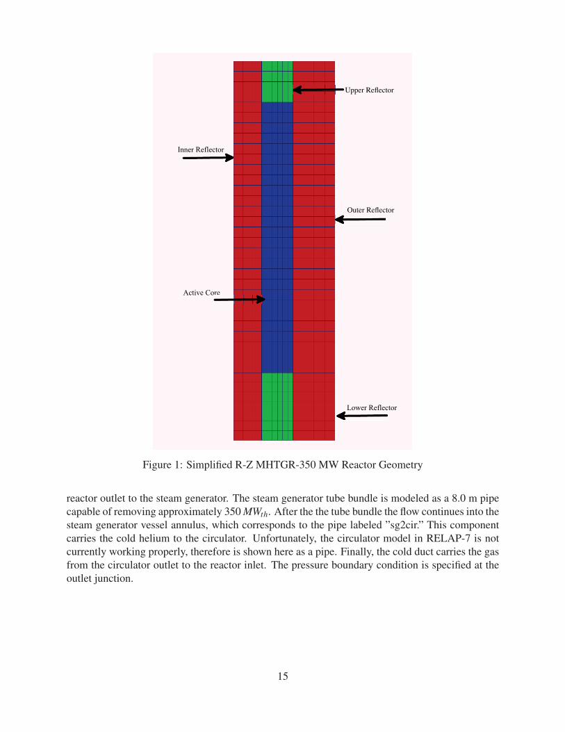
The original 3-D geometry with 1/3rd core symmetry was also simplified to a 2-D cylindrical
(R-Z) model. The layout of this simplified MHTGR-350 model is shown in Figure 1. The core
includes an inner reflector region, annular active core, top and bottom reflectors, and an outer
reflector region. The model is 11.1 m tall and 2.97 m in radius. The active core measures 7.9 m
in height and radially 0.92 m for the annular region width. The coolant flows directly into the top
reflector, followed by the active core, and, finally, the bottom reflector. Non-local heating effects
and radiation heat transfer are neglected.
From the pronghorn perspective the simulation entails a multi-physics steady state problem. There-
fore, given a set of boundary conditions from RELAP-7 the code solves a non-linear eigenvalue
problem. The cross sections for this model include the effects of the variations in fuel and mod-
erator temperature. The tracked parameters include: system pressure, core inlet temperature, core
outlet temperature, core fuel temperature distribution, core moderator temperature distribution,
core fluid temperature distribution, core power distribution, and local static pressure distribution.
3.2 RELAP-7 Geometry
The RELAP-7 model is entirely based on 1-D pipes and junctions. Figure 2 shows an schematic
of the system. The boundary conditions for temperature and velocity (or momentum) are specified
at the inlet junction. This is followed by the 5 m hot duct which carries the hot helium from the
14
Inner Reflector
������������
� ���������
Lower Reflector
Active Coreore
Figure 1: Simplified R-Z MHTGR-350 MW Reactor Geometry
reactor outlet to the steam generator. The steam generator tube bundle is modeled as a 8.0 m pipe
capable of removing approximately 350 MWth. After the the tube bundle the flow continues into the
steam generator vessel annulus, which corresponds to the pipe labeled ”sg2cir.” This component
carries the cold helium to the circulator. Unfortunately, the circulator model in RELAP-7 is not
currently working properly, therefore is shown here as a pipe. Finally, the cold duct carries the gas
from the circulator outlet to the reactor inlet. The pressure boundary condition is specified at the
outlet junction.
15

Figure 2: Relap-7 Plant System Layout
16

4 Numeric Method
The method of weighted residuals (or Galerkin procedure) is used to obtain the approximation
to the integral form of the PDEs. The weighted residual form of the equations is derived by
multiplying each term of the differential equations by a test function Ψ and integrating over the
volume. The final weak formulation is obtained by trading differentiation with the product rule.
The method of weighted residuals is used to formulate a nonlinear system of the form
F(U) = 0. (17)
This system is then solved iteratively via the JFNK method [9, 10]. The JFNK method is a com-
bination of the quadratically convergent Newton method and a Krylov subspace iterative method.
The first-order Taylor expansion of Eq. (17) about Um gives the following linear system,
JmδUm =−F(Um), (18)
where Jmi, j ≡ ∂Fi(Um)
∂Umj
is the i, j element of Jacobian matrix for the mth Newton iteration. The linear
system (18) is solved using a Krylov subspace method and the solution is updated as
Um+1 = Um +dδUm, (19)
where 0 < d ≤ 1 is a scalar damping parameter chosen adaptively to avoid unphysical solutions.
Because Krylov methods merely require matrix-vector products, a Jacobian-Free Newton-Krylov
(JFNK) method can be used to alleviate the explicit formation of the expensive Jacobian matrix.
In JFNK the matrix-vector product is approximated by the finite difference form,
Jv ≈ F(U+hv)−F(U)
h, (20)
where h is the perturbation parameter and v is provided by the Krylov method.
In PRONGHORN, the JFNK method is used to replace the upscattering iterations (the thermal and
fast neutron flux vectors are solved simultaneously), additionally a nonlinear Eigenvalue solver is
implemented in Pronghorn. This solver is “pre-conditioned” with the power iteration method in
which the fission source and Eigenvalue are fixed during the Krylov iterations. Previous work used
JFNK to treat coupled neutronics and thermal fluids problems or to solved the nonlinear scattering
problem in neutronics [11, 12].
17

5 Finite Element Discretization
5.1 RELAP-7 Model
The weak formulation that is associated with the RELAP-7 Model ( (1), (2), and (3)) leads to the
following nonlinear residual functions:
• Fluid Continuity Nonlinear Residual Function
Fρ (UUU) =
(∂ρ∂ t
,Ψ)−(
ρu,∂Ψ∂x
)+ 〈ρun̂x,Ψ〉Γ (21)
• Momentum Nonlinear Residual Function
Fρu (UUU) =
(∂ (ρu)
∂ t,Ψ
)− (ρgx,Ψ)+
(f
ρ2dh
|u|u,Ψ)−(
ρu2,∂Ψ∂x
)+
(P,
∂Ψ∂x
)+⟨ρu2n̂x,Ψ
⟩Γ + 〈Pn̂x,Ψ〉Γ (22)
• Energy Conservation Nonlinear Residual Function
Substituting ρuH = ρu(E + Pρ ) = u(ρE +P) in (3) and applying the Galerkin procedure
yields
FρE (UUU) =
(∂ (ρE)
∂ t,Ψ
)+(Hwaw(T −Tw),Ψ)+
(f
ρ2dh
|u|u2,Ψ)− (uρgx,Ψ) (23)
−(
ρuE,∂Ψ∂x
)−(
uP,∂Ψ∂x
)+ 〈ρuEn̂x,Ψ〉Γ + 〈uPn̂x,Ψ〉Γ
where
F = nonlinear residual function
U = (ρ,ρu,ρE)T
Ψ is a scalar test function
5.2 Pronghorn Model
The weak formulation that is associated with the Pronghorn equation set is obtained by applying
the method of weighted residuals to equations (7), (9), (10), (11), (12), and (13), respectively.
• Momentum Nonlinear Residual Function
Fρ�u(UUU) = (ε∇P,Ψ)− (ερ f�g,Ψ
)+(Wρ f�u,Ψ
)(24)
18

• Pressure Poisson Nonlinear Residual Function
FP(UUU) =
(∂∂ t
(εPRTf
),Ψ
)+
(ε2
W∇P,∇Ψ
)−(
ε2
Wρ f�g,∇Ψ
)
−⟨
ε2
W∇P,Ψ
⟩+
⟨ε2
Wρ f�g,Ψ
⟩(25)
• Fluid Energy Nonlinear Residual Function
FTf (UUU) =
(∂ερ f cp f Tf
∂ t,Ψ
)− (
ερ f cp f�uTf ,∇Ψ)+(εκ f ∇Tf ,∇Ψ
)+(α(Tf −Ts),Ψ
)+⟨ερ f cp f�uTf ,Ψ
⟩−⟨εκ f ∇Tf ,Ψ
⟩(26)
• Solid Energy Nonlinear Residual Function
FTs(UUU) =
(∂ (1− ε)ρscpsTs
∂ t,Ψ
)+(κse f f ∇Ts,∇Ψ
)+(α(Ts −Tf ),Ψ
)− (Q,Ψ)−⟨κse f f ∇Ts,Ψ
⟩(27)
• Neutron Diffusion Nonlinear Residual Function
Fφg(UUU) =
(1
vg
∂φg
∂ t,Ψ
)+(Dg∇φg,∇Ψ)−⟨
Dg∇φg,Ψ⟩+(Σrφg,Ψ)
−((1−β )χg ∑
g′νΣ f g′φg′ ,Ψ
)−(
∑g′,g′ �=g
Σg′→gs φg′ ,Ψ
)−(
∑k
χdg,kλkCk,Ψ
)(28)
• Delayed Neutron Precursor Nonlinear Residual Function
FCk(UUU) =
(∂Ck
∂ t,Ψ
)+(λkCk,Ψ)−
(∑g′
βk,g′νΣ f g′φg′ ,Ψ
)(29)
where
F = nonlinear residual function
U = (ρ�u,P,Tf ,Ts,φg,Ck)T
Ψ is a scalar test function
19

6 System Integration
6.1 Direct Coupling with Boundary Conditions
The integration of RELAP-7 and PRONGHORN is based on a loose coupling of the system,
whereby each application will use an independent mesh. A data exchange will be implemented
to couple the codes. This type of direct coupling has been successfully used in the past with the
TINTE time dependent core solver and the Flownex systems code[13, 14, 15]. To determine the
required parameters for the exchange we will look at the fluid boundary terms.
For the RELAP-7 model the coupling arises from the boundary terms of the fluid continuity, mo-
mentum, and fluid energy equations
〈ρun̂x,Ψ〉Γ⟨ρu2n̂x,Ψ
⟩Γ + 〈Pn̂x,Ψ〉Γ
〈ρuEn̂x,Ψ〉Γ + 〈uPn̂x,Ψ〉Γ
The corresponding boundary conditions for the RELAP-7 fluid medium are expressed as
P = PPHinlet ∈ ΓR7outlet
�n ·[− ε
W∇P+
ερ f�gW
]= (�n ·ρ�u)PHoutlet
∈ ΓR7inlet
Tf = TPHoutlet ∈ ΓR7inlet
where
PPHinlet is the inlet pressure pressure computed in PRONGHORN that will be imposed on the
RELAP-7 outlet boundary , ΓR7outlet
a fixed, uniform mass flow rate condition is set at the inlet boundary, ΓR7inlet
a fixed, uniform temperature from the PRONGHORN model, TPHoutlet , is set at the RELAP-7
inlet boundary, ΓR7inlet
For the PRONGHORN model the coupling arises from the boundary terms of the fluid pressure
and fluid energy equations
⟨ε2
W ∇P,Ψ⟩+⟨
ε2
W ρ f�g,Ψ⟩
⟨ερ f cp f�uTf ,Ψ
⟩−⟨εκ f ∇Tf ,Ψ
⟩20
Note that the momentum equation in the PRONGHORN model does not contain any boundary
terms. The conditions for this equation are imposed via the pressure Poisson equation. The corre-
sponding boundary conditions for the fluid medium are expressed as
P = PR7inlet ∈ ΓPHoutlet
�n ·[− ε
W∇P+
ερ f�gW
]= (�n ·ρ�u)R7outlet
∈ ΓPHinlet
Tf = TR7outlet ∈ ΓPHinlet
where
PR7inlet is the inlet pressure computed in RELAP-7 that will be imposed on the PRONGHORN
outlet boundary, ΓPHoutlet
a fixed, uniform mass flow rate condition is set at the inlet boundary, ΓPHinlet
a fixed, uniform temperature from RELAP-7 model, TR7out , is set at the inlet boundary,
ΓPHinlet
6.2 Helium Circulator
A helium circulator model is necessary to maintain system flow rate. Unfortunately, RELAP-7
does not currently include a circulator model. A simplified circulator was modeled by modifying
the boundary conditions.
The direct coupling boundary conditions for pressure in RELAP-7 are modified to
P =PPHinlet
CR∈ ΓR7outlet
where CR is the compression ratio of the helium circulator.
The direct coupling boundary conditions for temperature and inlet mass flow rate in PRONGHORN
are modified to
�n ·[− ε
W∇P+
ερ f�gW
]Ap = (�n ·ρ�u)R7outlet
Ap ∈ ΓPHinlet
Tf = TR7outletCRγ−1/γ ∈ ΓPHinlet
where
Ap is the cross sectional area of the pipe at the pronghorn inlet
γ =CpCv
, the ratio of specific heats
21
7 System Testing
7.1 Pronghorn Testing
Testing for the PRONGHORN calculation was done by solving for each physics (neutronics, heat
conduction, pressure and momentum, and fluid energy) separately. This was done by holding the
coupled values for the independent physics constant for each calculation. Once adequate con-
vergence behavior was achieved the convergence behavior of the tightly coupled problem was
examined. The final mesh and the order of the Lagrange shape functions used in the coupled
RELAP-7/PRONGHORN calculation were chosen such that reasonable spatial convergence of the
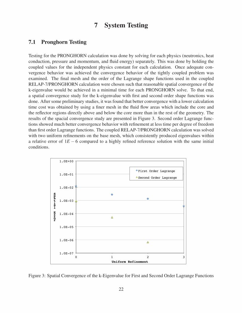
k-eigenvalue would be achieved in a minimal time for each PRONGHORN solve. To that end,
a spatial convergence study for the k-eigenvalue with first and second order shape functions was
done. After some preliminary studies, it was found that better convergence with a lower calculation
time cost was obtained by using a finer mesh in the fluid flow areas which include the core and
the reflector regions directly above and below the core more than in the rest of the geometry. The
results of the spacial convergence study are presented in Figure 3. Second order Lagrange func-
tions showed much better convergence behavior with refinement at less time per degree of freedom
than first order Lagrange functions. The coupled RELAP-7/PRONGHORN calculation was solved
with two uniform refinements on the base mesh, which consistently produced eigenvalues within
a relative error of 1E − 6 compared to a highly refined reference solution with the same initial
conditions.
1.0E-07�
1.0E-06�
1.0E-05�
1.0E-04�
1.0E-03�
1.0E-02�
1.0E-01�
1.0E+00�
0� 1� 2� 3�
Spatial
Error�
Uniform Refinement�
First Order Lagrange�
Second Order Lagrange�
Figure 3: Spatial Convergence of the k-Eigenvalue for First and Second Order Lagrange Functions
22
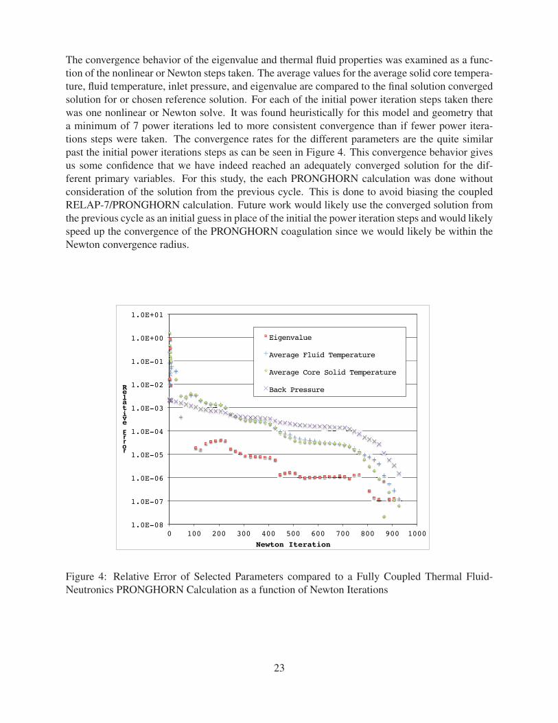
The convergence behavior of the eigenvalue and thermal fluid properties was examined as a func-
tion of the nonlinear or Newton steps taken. The average values for the average solid core tempera-
ture, fluid temperature, inlet pressure, and eigenvalue are compared to the final solution converged
solution for or chosen reference solution. For each of the initial power iteration steps taken there
was one nonlinear or Newton solve. It was found heuristically for this model and geometry that
a minimum of 7 power iterations led to more consistent convergence than if fewer power itera-
tions steps were taken. The convergence rates for the different parameters are the quite similar
past the initial power iterations steps as can be seen in Figure 4. This convergence behavior gives
us some confidence that we have indeed reached an adequately converged solution for the dif-
ferent primary variables. For this study, the each PRONGHORN calculation was done without
consideration of the solution from the previous cycle. This is done to avoid biasing the coupled
RELAP-7/PRONGHORN calculation. Future work would likely use the converged solution from
the previous cycle as an initial guess in place of the initial the power iteration steps and would likely
speed up the convergence of the PRONGHORN coagulation since we would likely be within the
Newton convergence radius.
1.0E-08�
1.0E-07�
1.0E-06�
1.0E-05�
1.0E-04�
1.0E-03�
1.0E-02�
1.0E-01�
1.0E+00�
1.0E+01�
0� 100� 200� 300� 400� 500� 600� 700� 800� 900� 1000�
Relative�������
Newton Iteration�
Eigenvalue�
Average Fluid Temperature�
Average Core Solid Temperature�
Back Pressure�
Figure 4: Relative Error of Selected Parameters compared to a Fully Coupled Thermal Fluid-
Neutronics PRONGHORN Calculation as a function of Newton Iterations
23

7.2 RELAP-7 Testing
A null transient (steady state) solution was obtained in RELAP-7 to ensure the proper function
of the various components, including the circulator, which is modeled via the pressure boundary
condition. The equation of state was also checked out with this first case. A fluid temperature of
862 K and a velocity 48 m/s were fixed at the inlet. The system pressure was fixed at the outlet
to 6.42 MPa and the compression ratio for the circulator was set to 1.01422. Results from this
simulation are included in Figure 5.
(a) Coolant Temperature [K] (b) Coolant Pressure [Pa]
(c) Coolant Density[
kgm3
](d) Coolant Velocity
[ms
]
Figure 5: Thermal-Physical Results from a RELAP7 System Calculation with a Null Transient
24
A simulation time of 1.07 seconds was more than necessary to achieve the steady state condition.
The execution time was 141 seconds on 7 processors. The fluid temperature remains constant until
it reaches the steam generator section after which it drops to 525 K. The system pressure, which
was set to 6.42 MPa at the boundary is decreased by the circulator model to 6.33E6. The pressure
drop across the loop, from the inlet to the circulator, is 0.13 MPa. The density reaches its peak in
the cold duct with a value of 5.83 kg/m3. The fluid velocity slows in the steam generator as the
fluid is cooled, but experiences a sudden increase in the cold duct section, due to the change in the
pipe area.
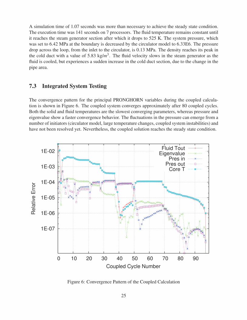
7.3 Integrated System Testing
The convergence pattern for the principal PRONGHORN variables during the coupled calcula-
tion is shown in Figure 6. The coupled system converges approximately after 80 coupled cycles.
Both the solid and fluid temperatures are the slowest converging parameters, whereas pressure and
eigenvalue show a faster convergence behavior. The fluctuations in the pressure can emerge from a
number of initiators (circulator model, large temperature changes, coupled system instabilities) and
have not been resolved yet. Nevertheless, the coupled solution reaches the steady state condition.
1E-07
1E-06
1E-05
1E-04
1E-03
1E-02
0 10 20 30 40 50 60 70 80 90
Rel
ativ
e E
rror
Coupled Cycle Number
Fluid ToutEigenvalue
Pres inPres out
Core T
Figure 6: Convergence Pattern of the Coupled Calculation
25

Figure 7 includes the PRONGHORN results as a function of coupled cycle and Figure 8 shows
the RELAP-7 results as a function of simulation time. The final eigenvalue is 0.983616 with an
average core temperature of 849 K. The strong negative feedback of the reactor can be seen in
the first cycles where the average core temperature increases and, consequently, produces a sharp
decrease in the core eigenvalue. The calculated temperature coefficient of reactivity for these first
cycles is −5x10⁻⁵Δk/k/oC, which is consistent with that of the MHTGR design at the end of
equilibrium cycle [16]. The average fluid temperature exiting the core is low, 860 K, and probably
due to low heat transfer coefficients. The RELAP-7 pressure plot in Figure 8(c) seems to indicate
that the sudden temperature increase in the early cycles induces an oscillation in the pressure
solution in the system. The oscillation dampens over time and the system finally reaches a stable
point.
0.9832
0.9834
0.9836
0.9838
0.984
0.9842
0.9844
0.9846
0.9848
0.985
0 10 20 30 40 50 60 70 80 90
K-e
ffect
ive
Coupled Cycle Number
(a) Eigenvalue
830
835
840
845
850
855
860
865
870
0 10 20 30 40 50 60 70 80 90
Tem
pera
ture
[K]
Coupled Cycle Number
Fluid outlet Average core
(b) Coolant and Core Temperatures [K]
6.4235
6.424
6.4245
6.425
6.4255
6.426
6.4265
6.427
6.4275
6.428
0 10 20 30 40 50 60 70 80 90
Inle
t Flu
id P
ress
ure
[MP
a]
Coupled Cycle Number
(c) Coolant Inlet Pressure [MPa]
3.56
3.58
3.6
3.62
3.64
3.66
3.68
3.7
0 10 20 30 40 50 60 70 80 90
Out
let F
luid
Den
sity
[kg/
m3 ]
Coupled Cycle Number
(d) Coolant Outlet Density[
kgm3
]
Figure 7: PRONGHORN Coupled Calculation Results
The flux and heat source distributions are included in Figure 9. The fast flux in Figure 9(a) is
mainly constraint near the active core region whereas the thermal flux in Figure 9(b) displays the
typical double radial hump, that is characteristics of the MHTGR’s annular core with inner and
26

(a) Coolant Outlet Temperature [K] (b) Coolant Inlet Pressure [Pa]
(c) Coolant Outlet Momentum[
kgm2s
]
Figure 8: RELAP-7 Coupled Calculation Results
outer reflectors. The fission heat source in Figure 9(c) shows a peak near the inner reflector, which
corresponds to the large thermal flux peak in the reactor core caused by the inner reflector region.
In addition, the flux and fission heat source distributions display a top peaked shape that is driven
by the temperature distribution (shown in 10(b)). Since the flow in the reactor originates at the top
and proceeds down through the core it creates a cooler fuel region in upper portion of the core.
Other relevant thermo-physical distributions of the MHTGR R-Z core model are shown in Figure
10. As previously mentioned, the coolant temperature distribution is low for the reactor design.
The pressure drop across the reactor 40 kPa, which is 15 percent higher than the nominal 34 kPa.
The RELAP-7 time dependent results are included in Figure 8. The plots show similar patterns to
those in PRONGHORN. All of the coupling variables (outlet temperature, inlet pressure and outlet
momentum) appear to stabilize. The RELAP-7 distributions shown in Figure 11 are very similar
to those obtained with the original null transient problem used during stand alone testing.
27

(a) Scaled Fast Flux (b) Scaled Thermal Flux
(c) Normalized Fission Heat Source
Figure 9: Neutronics Results From the Final PRONGHORN Core Calculation
28

(a) Coolant Temperature [K] (b) Homogenized Solid Temperature [K]
(c) Coolant Density[
kgm3
](d) Coolant Pressure [Pa]
Figure 10: Thermal Physical Results from the Final PRONGHORN Core Calculation
29

(a) Coolant Temperature [K] (b) Coolant Pressure [Pa]
(c) Coolant Density[
kgm3
](d) Coolant Velocity
[ms
]
Figure 11: RELAP-7 Distributions from the Coupled Calculation
30
8 Conclusion
The RELAP-7 and PRONGHORN applications have been successfully coupled using an opera-
tor split approach. The results show that the coupled system correctly converges to the steady
state condition. All final distributions contain the characteristics of the MHTGR design. The con-
vergence pattern shows good behavior for the exception of some initial pressure oscillations that
eventually dampen. The source of the oscillations is currently undetermined, but various possibil-
ities have been identified. There were significant difficulties with the modeling of a circulator in
RELAP-7 and the effects of the component were simulated by use of modified boundary conditions
in the coupled system.
31

9 Future Work
The successful coupling of RELAP-7 and PRONGHORN code was possible because of the use of
the MOOSE framework. However, the code used to couple RELAP7 and PRONGHORN is cur-
rently available only as a prototype which demonstrates how to tie the codes together and exchange
the information between them. More work is required to turn this prototype into a production code,
which is possible given available funds and personnel within a short period of time.
32

References
[1] D. Andrs, R. Berry, D. Gaston, R. Martineau, J. Peterson, H. Zhang, H. Zhao, and L. Zou.
Relap-7 level 2 milestone report: Demonstration of a steady state single phase pwr simlula-
tion with relap-7. Technical report, Idaho National Laboratory, 2012.
[2] H. Park, D.A. Knoll, D.R. Gaston, and R.C. Martineau. Toghly coupled multiphysics algo-
rithms for pebble bed reactors. Nuclear Engineering and Design, 166:118–133, April 2010.
[3] Satish Balay, Kris Buschelman, Victor Eijkhout, William D. Gropp, Dinesh Kaushik,
Matthew G. Knepley, Lois Curfman McInnes, Barry F. Smith, and Hong Zhang. PETSc
users manual. Technical Report ANL-95/11 - Revision 2.1.5, Argonne National Laboratory,
2004.
[4] Benjamin S. Kirk, John W. Peterson, Roy H. Stogner, and Graham F. Carey. libMesh: a C++
library for parallel adaptive mesh refinement/coarsening simulations. Eng Comput-Germany,
22(3-4):237–254, January 2006.
[5] Shijie Liu and Jacob H. Masliyah. Handbook of Porous Media. Taylor & Francis, Boca
Rotan, Florida, 2005.
[6] F Reitsma, K Ivanov, T Downar, H de Hass, S Sen, G Strydom, R Mphahlele, B Tyobeka,
V Seker, H Gougar, and H Lee. PBMR coupled neutronics/thermal hydraulics transient
benchmark the PBMR-400 core design. Technical Report NEA/NSC/DOC(2007) Draft-V07,
OECD/NEA/NSC, 2007.
[7] J. Ortensi, D. Andrs, A.A. Bingham, R. Martineau, and J. Peterson. Relap-7 and pronghorn
initial integration plan. Technical Report INL/EXT-12-26016, Idaho National Laboratory,
May 2012.
[8] J. Ortensi. Prismatic core coupled transient benchmark. Trans. Amer. Nuc. Soc., June 2011.
[9] P. N. Brown and Y. Saad. Hybrid krylov methods for nonlinear systems of equations. SIAMJ. Sci. Stat. Comput., 11(3):450, 1990.
[10] D.A. Knoll and D.E. Keyes. Jacobian-free newtown-krylov methods: A survey of approaches
and applications. J. Comput. Phys., 193(2):357, 2004.
[11] D.F. Gill and Y.Y. Azmy. A Jacobian–free Newton–Krylov iterative scheme for criticality
calculations based on the neutron diffusion equation. In American Nuclear Society 2009International Conference on Advances in Mathematics, Computational Methods, and ReactorPhysics, Saratoga Springs, NY, May 3–7 2009.
[12] V. Mahadevan and J. Ragusa. Novel hybrid scheme to compute several dominant eigenmodes
for reactor analysis problems. In International Conference on the Physics of Reactors, Inter-
laken, Switzerland, September 14–19 2008.
33

[13] H. Gerwin, W. Scherer, A. Lauer, and I. Clifford. Tinte – nuclear calculation theory de-
scription report. Technical Report ISSN 0944-2952, Institute For Energy Reseach, January
2010.
[14] P.G. Rousseau, C.G. Du Toit, and W.A. Landman. Validation of a transient thermal-fluid
systems cfd model for a packed bed high temperature gas-cooled nuclear reactor. NuclearEngineering and Design, 236:555–564, 2006.
[15] D. Marais. Validation of the point kinetic neutronic model of the pbmr. Master’s thesis,
North-West University, 53 Borcherd Street, Potchefstroom, 2531, South Africa, May 2007.
[16] R.F. Turner, A.M. Baxter, O.M. Stansfield, and R.E. Vollman. Annular core for the modular
high-temperature gas-cooled reactor (mhtgr). Nuclear Engineering and Design, (109):27–
231, 1988.
[17] A. Narasimhan and J L. Lage. Modified hazen-dupuit-darcy model for forced convection of a
fluid with temperature dependent viscoisty. Journal of Heat Transfer, 123(38):31–38, 2000.
34

Top Related