


Languages
Pages
Legal

NREL is a national laboratory of the U.S. Department of Energy, Office of Energy Efficiency and Renewable Energy, operated by the Alliance for Sustainable Energy, LLC.
Infrastructure Analysis Tools: A Focus on Cash Flow Analysis
Marc Melaina, Michael PenevNational Renewable Energy Laboratory
Presented at the Hydrogen Infrastructure MeetingInternational Council for Clean Transportation (ICCT) Breakthrough Technologies Institute (BTI)Toronto, 5 June 2012
NREL/PR‐5600‐55563
This presentation does not contain any proprietary, confidential, or otherwise restricted information
2
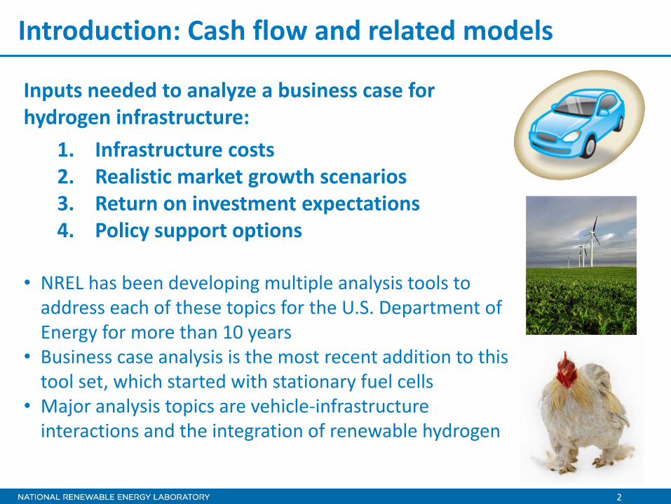
Introduction: Cash flow and related models
Inputs needed to analyze a business case for hydrogen infrastructure:
1. Infrastructure costs2. Realistic market growth scenarios3. Return on investment expectations4. Policy support options
• NREL has been developing multiple analysis tools to address each of these topics for the U.S. Department of Energy for more than 10 years
• Business case analysis is the most recent addition to this tool set, which started with stationary fuel cells
• Major analysis topics are vehicle‐infrastructure interactions and the integration of renewable hydrogen

3
Main models supporting cash flow analysis
Hydrogen Analysis (H2A) models • Production, Delivery, and Fuel Cells• Discounted cash flow framework • Models are transparent and public
http://www.hydrogen.energy.gov/h2a_analysis.html
Scenario Evaluation and Regionalization Analysis (SERA) Model• Optimizes spatial‐temporal infrastructure in response to hydrogen demand
• Runs have optimized on least cost $/kg• H2A cost models “plug in” to SERA• Optimization across all pathway options• Developed over ~7 years• Sub‐models explore finance options
Fuel cell vehicle market projections (ADOPT, MA3T, other models)• Based upon consumer preferences and vehicle attributes• Market share models haven’t been integral to SERA runs

4
1. Determining infrastructure costs Combining unit costs with detailed geographic constraints improves the realism of infrastructure cost estimates• Methodologically, this is done by ingesting H2A unit costs into the spatial‐temporal optimization routine within SERA
KEY MODELING FACTORS TO CONSIDERFull supply chain costs • Multiple production, storage and delivery options (H2A)• Resource availability and cost (wind, biomass, etc.)
(based upon multiple data sources)• Natural gas pathways tend to dominate (H2A‐SERA)
Station costs • Station types are coupled to delivery options (H2A)• Coverage is based upon station numbers and size
distribution (SERA)• Coverage evolves on a city‐by‐city basis, requiring a
detailed geographic cost model (SERA)Discounted cash flow framework (H2A‐SERA)• H2A framework assumes 10% IRR to calculate a
“profited cost” (H2A)• SERA financial analysis is more flexible and business‐
oriented (SERA)
Pathway combinations in SERA
Example of SERAdeliveryresults

5
2. Realistic market growth scenarios• Steady‐state infrastructure costs are relatively simple to analyze; rollout dynamics are much more complex
• For early market growth dynamics and interactions, NREL analysts have incorporated guidance from: • Stakeholder workshops (Greene et al. 2008)• Early market coordination activities such as the Hawaii Hydrogen Initiative (H2I), EIN, and CaFCP
• Initial discussions with CCAT• Station rollout is explicit at any level of detail• SERA offers a consistent framework to incorporate regional infrastructure rollout scenarios
Bay Area,
CA
Chicago, IL
Station sizes
New FCEV sales Annual cash flow @ $8/kg
6
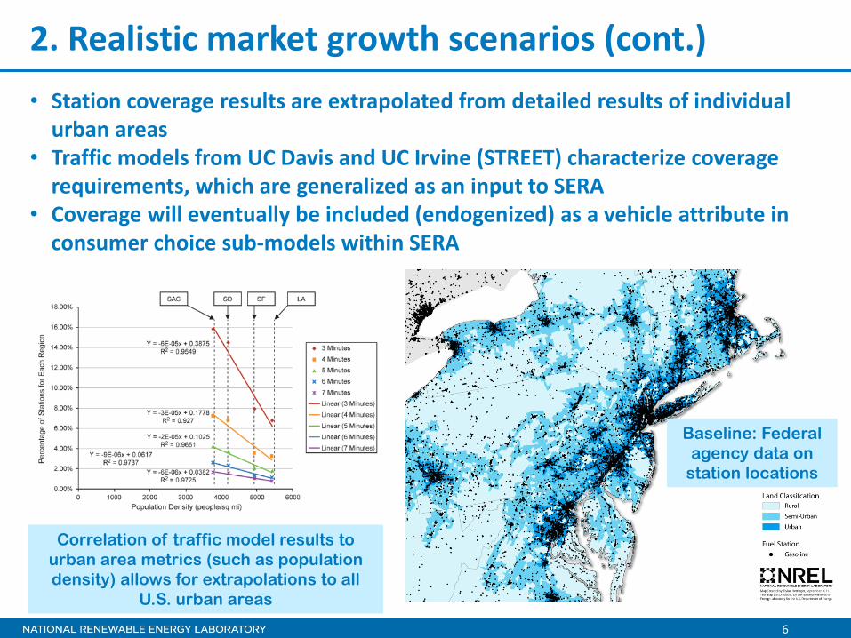
2. Realistic market growth scenarios (cont.)• Station coverage results are extrapolated from detailed results of individual urban areas
• Traffic models from UC Davis and UC Irvine (STREET) characterize coverage requirements, which are generalized as an input to SERA
• Coverage will eventually be included (endogenized) as a vehicle attribute in consumer choice sub‐models within SERA
Baseline: Federal agency data on
station locations
Correlation of traffic model results to urban area metrics (such as population density) allows for extrapolations to all
U.S. urban areas

7
Basic national cash flow results from SERA• Break‐even year is a function of assumed market price ($/kg)• Cash flows determined nationally, by state, by city, or per station
Zero cumulative cash flow is achieved between 2018 and 2025 if hydrogen is priced at
$11.00/kg or $6.75/kg

8
More elaborate and detailed cash flows
• Developed in response to partner/stakeholder requirements in H2I and discussions with EIN/CaFCP
• Hydrogen price assumed to be equal to gasoline price on a per‐mile‐driven basis (need mpg assumptions to determine)
• Short‐fall results from high fixed costs and underutilization of infrastructure in early years
$‐
$1
$2
$3
$4
$5
Millions
Financing
Maintenance
Labor
Utilities
Feedstock
Revenue
Mon
thly Cash Flow
s
Analysis Period
Expenses & Revenue Projections vs. Year
$‐
$1
$2
$3
$4
$5
Millions
Financing
Maintenance
Labor
Utilities
Feedstock
Revenue
Mon
thly Cash Flow
s
Analysis Period
Expenses & Revenue Projections vs. Year
Revenue short‐fall (barrier to market entry)
9
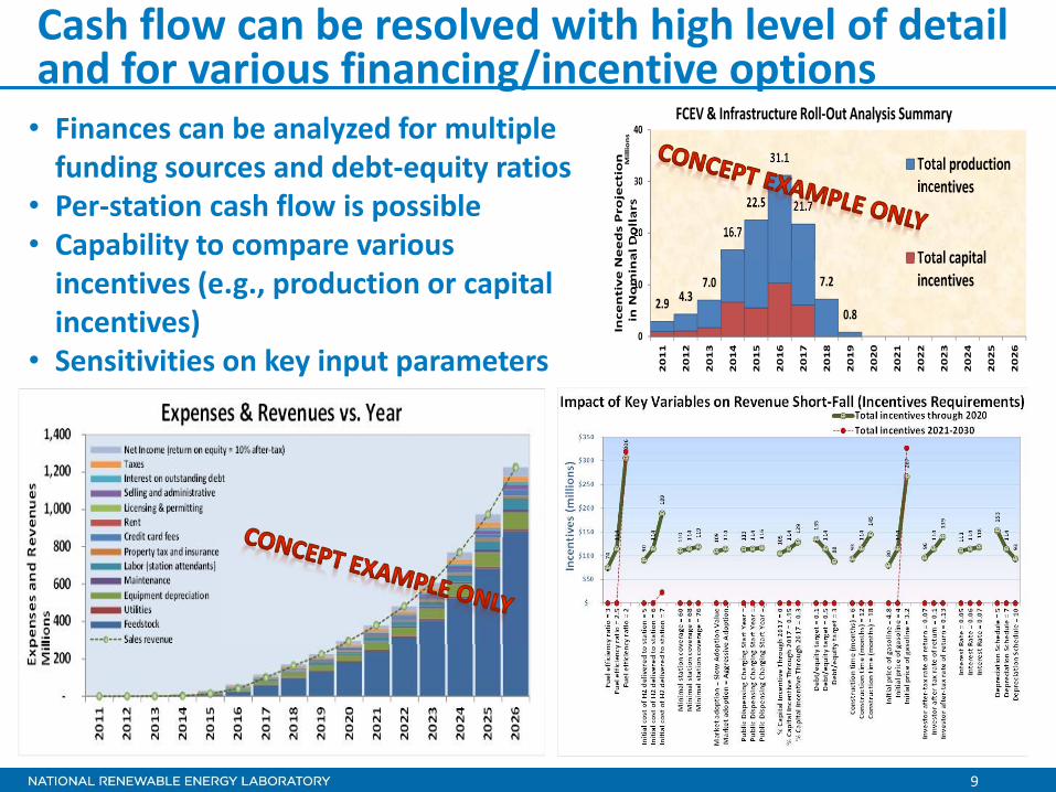
Cash flow can be resolved with high level of detail and for various financing/incentive options
2.9 4.37.0
16.7
22.5
31.1
21.7
7.2
0.80
10
20
30
40
2011
2012
2013
2014
2015
2016
2017
2018
2019
2020
2021
2022
2023
2024
2025
2026
Millions
Total productionincentives
Total capitalincentives
IncentiveNeeds Projection
in Nominal Dollars
FCEV & Infrastructure Roll‐Out Analysis Summary• Finances can be analyzed for multiple funding sources and debt‐equity ratios
• Per‐station cash flow is possible• Capability to compare various incentives (e.g., production or capital incentives)
• Sensitivities on key input parameters
10
SummaryNREL models• NREL has developed and maintains a variety of infrastructure analysis models for the U.S. Department of Energy
• Business case analysis has recently been added to this tool set
Cash flow analysis• Cash flows depend upon infrastructure costs, optimized spatially and temporally, and assumptions about financing and revenue
• Detailed metrics have been incorporated on financing/incentives
Next steps in modeling• Continue to collect feedback on regional/local infrastructure development activities and “roadmap” dynamics
• Incorporate consumer preference assumptions on infrastructure to provide direct feedback between vehicles and station rollout

12
Additional Slides

13
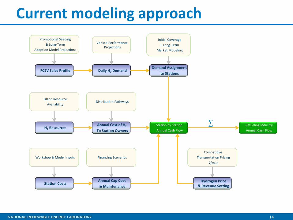
SERA overview The SERA Model integrates assumptions and data from multiple sources and related modeling efforts
14
Current modeling approach
FCEV Sales Profile Daily H2 Demand
Vehicle Performance Projections
Demand Assignment to Stations
Promotional Seeding& Long‐Term
Adoption Model Projections
Initial Coverage+ Long‐Term
Market Modeling
Station by Station Annual Cash Flow
H2 Resources
Island ResourceAvailability
Annual Cost of H2
To Station Owners
Distribution Pathways
Station Costs
Workshop & Model Inputs
Annual Cap Cost & Maintenance
Financing Scenarios
Refueling IndustryAnnual Cash Flow
∑
Hydrogen Price& Revenue Setting
Competitive Transportation Pricing
¢/mile

15
On‐going effort
FCEV Sales Profile Daily H2 Demand
Vehicle Performance Projections
Demand Assignment to Stations
Promotional Seeding& Long‐Term
Adoption Model Projections
Initial Coverage+ Long‐Term
Market Modeling
Station by Station Annual Cash Flow
H2 Resources
Island ResourceAvailability
Annual Cost of H2
To Station Owners
Distribution Pathways
Station Costs
Workshop & Model Inputs
Annual Cap Cost & Maintenance
Financing Scenarios
Refueling IndustryAnnual Cash Flow
∑
Hydrogen Price& Revenue Setting
Competitive Transportation Pricing
¢/mile
Introduce sales projectionsbased on:• Station coverage• Fueling costs• Vehicle prices• Vehicle size• Vehicle acceleration

16
Station roll‐out in support of FCEV
Station size and distribution modeled statistically to comply to gasoline demand distributionLarge stations as much 4,500 kg/day will be needed by 2025 as demand density grows

17
Sensitivity analysis74
114
306
90
114
189
110
114
119
109
114
113
114
116
105 114 129 135
114
88 93
114
145
80
114
267
96
114 13
9
111
114
118
153
114
93
$‐
$50
$100
$150
$200
$250
$300
$350Fuel efficiency ratio
= 3
Fuel efficiency ratio
= 2.5
Fuel efficiency ratio
= 2
Initial cost o
f H2 de
livered
to statio
n = 5
Initial cost o
f H2 de
livered
to statio
n = 6
Initial cost o
f H2 de
livered
to statio
n = 7
Minim
al statio
n coverage
= 60
Minim
al statio
n coverage
= 68
Minim
al statio
n coverage
= 76
Market a
doption = Slow
Ado
ption Va
lue
Market a
doption = Ag
gressive Ado
ption…
Public Dispe
nsing Ch
arging
Start Year =
…Pu
blic Dispe
nsing Ch
arging
Start Year =
…Pu
blic Dispe
nsing Ch
arging
Start Year =
…
% Cap
ital Incen
tive Th
roug
h 20
17 = 0
% Cap
ital Incen
tive Th
rough 20
17 = 0.15
% Cap
ital Incen
tive Th
roug
h 20
17 = 0.3
Deb
t/eq
uity ta
rget = 0.1
Deb
t/eq
uity ta
rget = 0.5
Deb
t/eq
uity ta
rget = 3
Constructio
n tim
e (m
onths) = 6
Constructio
n tim
e (m
onths) = 12
Constructio
n tim
e (m
onths) = 18
Initial pric
e of gasoline = 4.8
Initial pric
e of gasoline = 4
Initial pric
e of gasoline = 3.2
Investor after‐tax ra
te of return = 0.07
Investor after‐tax ra
te of return = 0.1
Investor after‐tax ra
te of return = 0.13
Interest Rate = 0.05
Interest Rate = 0.06
Interest Rate = 0.07
Dep
reciation Sche
dule = 5
Dep
reciation Sche
dule = 7
Dep
reciation Sche
dule = 10
Total incentives through 2020Total incentives 2021‐2030
Incentives
(millions)
Impact of Key Variables on Revenue Short‐Fall (Incentives Requirements)
Most important controllable variable: vehicle fuel economy‐ High fuel economy = lower infrastructure investment‐ High fuel economy = higher revenue per kg H2‐ High fuel economy = effective production resource utilization

18
0
1000000
2000000
3000000
4000000
15 20 25 30 40 50
Annu
al Sales
Fuel Economy (MPG)
Sales By MPG(listed by max in bin)
Actual
Model
0.0%
5.0%
10.0%
15.0%
20.0%
Actual Model
Percent HEV Sales
ADOPT matches historical sales
0
1000000
2000000
3000000
4000000
5000000
12 9 7
Annu
al Sales
Max Bin Accel Time (secs 0‐60 MPH)
Sales By Acceleration
Actual
Model0
1000000200000030000004000000
Annu
al Sales
Vehicle Price (MSRP)
Sales By MSRP (listed by max in bin)
Actual
Model0
5000001000000150000020000002500000
Annu
al Sales
Sales By Class
Actual
Model
0%
20%
40%
60%
80%
100%
National Model
HEV Buyers with Income Over $100k
$‐
$50,000
$100,000
$150,000
National Model
Average Income of HEV Buyers
• ADOPT has been calibrated for U.S. markets• Model predicts historical sales with a relatively high degree of accuracy• Range of FCEV sizes and performances will be modeled to provide wide variety of market choices
19
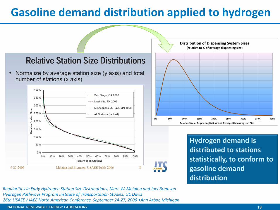
Gasoline demand distribution applied to hydrogen
Regularities in Early Hydrogen Station Size Distributions, Marc W. Melaina and Joel BremsonHydrogen Pathways Program Institute of Transportation Studies, UC Davis26th USAEE / IAEE North American Conference, September 24‐27, 2006 •Ann Arbor, Michigan
0% 50% 100% 150% 200% 250% 300% 350% 400%
Distribution of Dispensing System Sizes(relative to % of average dispensing size)
Relative Size of Dispensing Unit as % of Average Dispensing Unit Size
0% 50% 100% 150% 200% 250% 300% 350% 400%
Distribution of Dispensing System Sizes(relative to % of average dispensing size)
Relative Size of Dispensing Unit as % of Average Dispensing Unit Size
Hydrogen demand is distributed to stations statistically, to conform to gasoline demand distribution
Top Related