


Languages
Pages
Legal

ISSN: 2277-9655
[Thamer* et al., 5(12): December, 2016] Impact Factor: 4.116
IC™ Value: 3.00 CODEN: IJESS7
http: // www.ijesrt.com © International Journal of Engineering Sciences & Research Technology
[613]
IJESRT INTERNATIONAL JOURNAL OF ENGINEERING SCIENCES & RESEARCH
TECHNOLOGY
INFLUENCE OF MOVING LOADS ON CURVED BRIDGES Thamer A. Z*, Jabbbar S. A
* Collage of Engineering, Basrah University, Civil Engineering Department
Collage of Engineering, Basrah University, Civil Engineering Department
DOI: 10.5281/zenodo.205871
ABSTRACT The behavior of a curved slab bridge decks with uniform thickness under moving load is investigated in this study.
Three radii of curvature "R" are used (25, 50 and 75m) along with the straight bridge, R = ∞. The decks are simply
supported or clamped along the radial edges and free at the circular edges. The AASHTO[1] standard axle load
of the truck H20-44 is used and assumed to move in three track positions on the bridge. The finite element method
is employed for the analysis and the ANSYS 5.4 computer program is used for modelling and solving the cases
studied. Six different velocities (with a time required to pass the bridge ranging from 0.4 to 2.4 of the natural
period of the bridge) are used to investigate the velocity effect of the selected truck on the behavior of the bridge.
All the results obtained (stresses and vertical displacements) at mid-span are normalized to the corresponding
results of the static load. Results show that the maximum effect reached when the load crossing the bridge in a
time (66% to 80%) of the natural period of the bridge. The increase in central displacement due to a combined
effect of curvature and velocity is up to 1.75 times the static displacement, while a higher increase obtained for
shear stresses.
KEYWORDS: curved Bridge, moving load, finite element, AASHTO standard load, load velocity effect, ANSYS
program.
INTRODUCTION Horizontally curved bridges are commonly used in highway interchange areas. The increase in usage of such
structures is due to economical, aesthetical, architectural and engineering limitations. Bridge structures have been
mainly designed to prevent failure under static loads. The static response of bridge structure can be obtained quite
satisfactorily by different analysis techniques. The dynamic response of bridges due to moving loads is not easy
to predict. Most of existing design codes, such as AASHTO, take the dynamic effect into account by increasing
the static design loads by an impact factor "I", which is a function of span length only[1,2]. Different studied cases
on bridge's dynamic response showed that the real dynamic effect differs from that obtained by multiplying the
static effect by a dynamic impact factor "I" [8].
The dynamic study of bridge-vehicle interaction has been conducted theoretically and experimentally for many
years due to its importance and difficulty. The existence of moving mass makes the problem more difficult because
of the fact that acting forces varies in time and space. The investigation of this problem results in a large number
of publications.
Dey and Balascbramanian (1982) [10], investigated the dynamic response of horizontally curved bridge decks with
orthotropic elastic properties and simply supported along the radial edges under the action of a moving vehicle by
using a finite strip method. Dynamic deflections and moments were presented for the mid-point of the bridge
deck.
Lee, Duen, and Chung (1987)[12] ,carried out both static and dynamic tests on an old reinforced concrete bridge
prior to its demolition. The purpose of the static test was to calibrate the mathematical model used in the structural
analysis. The revised mathematical model was used to calculate the natural frequencies of the bridge deck. The
results compared reasonably well with the measured frequencies from the dynamic test. The study demonstrated
that within the design load range, the moment of inertia of a reinforced concrete bridge deck can be taken as that
ISSN: 2277-9655
[Thamer* et al., 5(12): December, 2016] Impact Factor: 4.116
IC™ Value: 3.00 CODEN: IJESS7
http: // www.ijesrt.com © International Journal of Engineering Sciences & Research Technology
[614]
of the plain concrete section. The effect of steel reinforcement and concrete cracking tend to compensate each
other and may therefore be ignored.
Austin and Lin (1996) [4] ,used three-dimensional finite element model to analyze a two-span highway bridge with
one end hinged support and the other end roller support. The influence line of mid-span displacements caused by
a 1000kip concentrated moving load along the outer girders was computed.
Barefoot et al (1997) [5], investigated the validation of the finite element models by ANSYS 5 program to predict
the static and dynamic response of steel girder bridges through comparison with field test data of a typical bridge.
A well accepted comparable results were obtained.
Challal and Shahawy (1998)[7], provided a state of the art review on dynamic testing procedure for bridges with
special emphasis on experimental evaluation of the dynamic amplification factor (DAF). The evaluation of (DAF)
was also provided in terms of different parameters like fundamental frequency, damping characteristics of the
bridge, road way roughness, vehicle speed, bridge geometry, construction materials and wheel dynamic load
measurement. Very stiff bridges were more influenced by vehicle mechanical properties than most modern less
stiff highway bridges.
Broquet (1999) [6], describes a parametric study to investigate the distribution of the dynamic amplification factors
throughout a bridge deck slab, based on the simulation of bridge-vehicle interaction. A three dimensional finite
element model was employed to represent the bridge structure. And the vehicle was represented by a system of
lumped masses. For the simulation of the dynamic effects, vehicle speed was varied between 40 and 120 km/h.
with trajectories either centered on, or at the edge of the deck slab. The dynamic amplification factor was higher
in the first span of a continuous bridge. An increase in vehicle weights led to a decrease in (DAF).
Martin et al (2000)[13], developed a finite element model of a typical bridge structure by using ANSYS program.
The relative influence of various design and load parameters was investigated using element model of a section
of an actual bridge. Mid-span displacement of the bridge was calculated and normalized with respect to the static
displacement. The most important factors affecting dynamic response were the basic flexibility of the structure
and more specifically, the relationship between the natural frequency of the structure and the exciting frequency
of the vehicle.
Jawad (2005) [11], studied the dynamic behavior of concrete bridge decks due to moving vehicles. Three
dimensional models of bridge decks were implemented within the finite element method using ANSYS 5.4
computer program. Dynamic amplification factors were evaluated at certain locations on the bridge for vertical
displacement, normal stress in longitudinal direction and shear stress in the transverse direction. Numerical results
showed a general trend for higher values than those specified by the AASHTO design code.
Dakheel (2007) [9], used the finite element method and thin plate theory to analyze a skew bridges (with different
skew angles) subjected to moving loads. The bridges structures were modeled using ANSYS 5.4 computer
program. The effects of single and dual wheel loads were studied by taking different load velocities. It was found
that increasing the skew angle of the bridge lead to reduction in the calculated deflection and bending stresses and
increase in the shear stresses. Increasing load speed resulted in increasing the dynamic amplification factor (DAF).
In the current research, the thin plate theory is employed to represent the curved bridge deck and analyzed for the
effect of the variation of the truck load in location and speed on the deflection and stresses of the bridge deck.
FINITE ELEMENT MODELING The bridge deck is simulated by using the shell 93 element which is an eight nodes quadrilateral shell element
with both bending and membrane capabilities [2]. The element has six degrees of freedom at each node: translations
in nodal x, y, and z directions and rotations about the nodal x, y, and z axes. The H20-44, truck design loading
contained in the Standard American Association of State Highway and Transportation Officials (AASHTO)
specification is used to simulate the moving vehicle. It represents two axels truck with total weight of 20 U.S.
tones (180 kN)[1]. The front axle is assumed to carry 20% of the weight and the rear axle the remaining 80%. The
truck and its configuration are shown in figure 1.

ISSN: 2277-9655
[Thamer* et al., 5(12): December, 2016] Impact Factor: 4.116
IC™ Value: 3.00 CODEN: IJESS7
http: // www.ijesrt.com © International Journal of Engineering Sciences & Research Technology
[615]
Figure (1): H20-44 AASHTO standard truck.
A programming capability in ANSYS called (the parametric design language) is implemented to simulate the load
movement from node to the next node.
CASES STUDIED The dynamic response of curved bridges with different radii of curvatures (R= 25, 50, and 75m) are studied. The
plan view of the bridge is shown in figure (2). To investigate the effects of curvature on the displacements and
stresses in the bridge, the resulted displacements and stresses from the analyses of the curved bridges are compared
to those of a right bridge having similar width and central length. Also, two cases of boundary conditions are
considered (simply supported or fixed) on both radial sides while the other sides are free. Moving axle load is
applied in the study with different velocities (V) and track positions to evaluate the effect of these parameters on
the results (displacements and stresses). The velocities are ranged between 20km/h to 120km/h ( V/Vf = 0.4 to 2.5
where V is the velocity of the vehicle and Vf is the velocity of the vehicle when crossing the bridge in a time
equals to the bridge natural period ) , the track positions are as shown in figure (3).
Figure 2: Plan view of curved bridge.
1- At the inner quarter line (2m from and parallel to the center line of the curved bridge.
2- At the center line of the curved bridge.
3- At the outer quarter line (2m from and parallel to the center line of the curved bridge).
All results are normalized to those of static load (applied at mid-span, same track) to evaluate the effect
of velocities of the load on the bridge at five points lie on the mid-span of the curved bridge, denoted by Pi where
i=1, 2,3,4,5 as shown in figure (3).
Figure 3: Positions of a- load tracks, b- points where the effects (displacements and stresses) are calculated.
The material properties used for the bridge slab in the analysis are listed in Table 1.
ISSN: 2277-9655
[Thamer* et al., 5(12): December, 2016] Impact Factor: 4.116
IC™ Value: 3.00 CODEN: IJESS7
http: // www.ijesrt.com © International Journal of Engineering Sciences & Research Technology
[616]
Table (1): Properties of the material of the bridge
Property Value
Density of concrete 2380kg/m3
Modulus of elasticity of concrete
(based on the ACI formula Ec = 4730√f' for
normal weight concrete)
21.52x10³ MPa
Poisson's ratio 0.25
Damping ratio 2%
ANALYSIS AND RESULTS To predict the effects of thickness on the response of the bridge, three thickness of the bridge slab are studied
(40cm, 60cm, and 80cm) which resulted in a thickness to length ratios of (0.033, 0.05, and 0.066).
The analysis implemented in three steps, in the first step the load is applied statically to evaluate the static effect
at mid-span. In the second step, the modal analysis of the structure is conducted to evaluate the fundamental
natural periods and use them for the third step. The third step is done by applying the moving loads on the bridge.
The fundamental periods (Tf) and the velocity of the axel load (Vf) that would pass the bridge in time Tf for the
slab with thickness 40cm are listed in Table 2.
Table (2): Fundamental periods for bridge models, plate thickness = 40cm. simply supported bridge.
Radius (m) Fundamental
period Tf (sec.)
Velocity Vf
km/h
25 0.9 47.92
50 0.85 50.84
75 0.84 51.44
∞ 0.83 51.95
The results of the analysis are given in the following figures:
1- The effect of truck velocity and location on the normal displacement of the bridge at mid-span (point 3) is given
in figure 4 (radii of curvature 25m)
2- The effect of truck velocity and location on the transverse stress (Sx) of the bridge at mid-span (point 3) is
given in figure 5 (radii of curvature 25m).
3- The effect of truck velocity and location on the longitudinal stress (Sy) of the bridge at mid-span (point 3) is
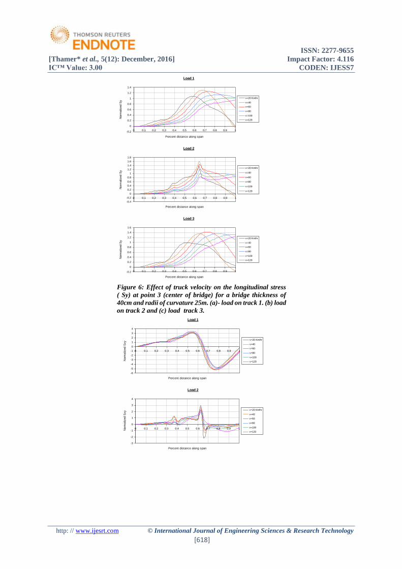
given in figure 6 (radii of curvature 25m)
4- The effect of truck velocity and location on the shear stress of the bridge (Sxy) at mid-span (point 3) is given
in figure 7 (radii of curvature 25m).
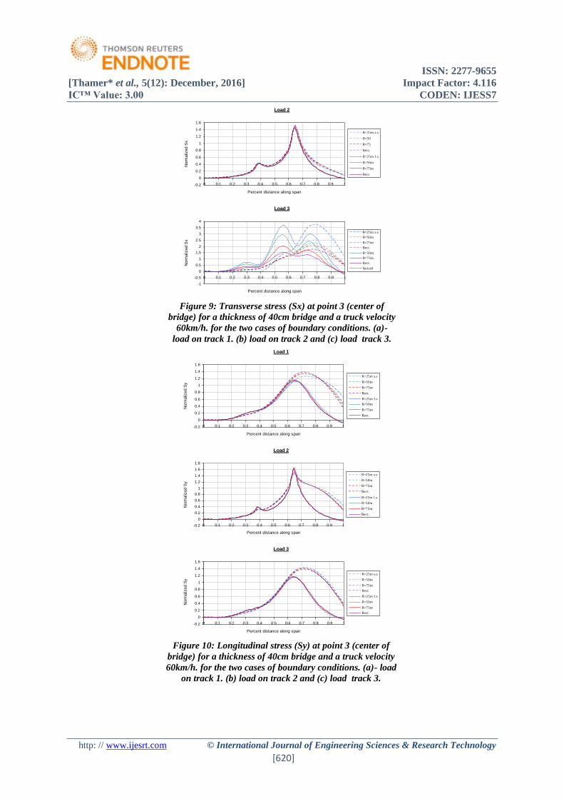
5- The effect of the type of the radial boundary conditions on the central displacement, transverse stress (Sx),
longitudinal stress (Sy) and shear stress (Sxy) of the bridge (for a vehicle velocity of 60km/h) on the three radii
of curvatures 25,50 and are given in figures 8,9,10 and 11 respectively.
6- The effect of the bridge slab thickness on the displacement and stresses are given in figure 12.
7- Comparisons of the maximum displacement along the center of span for all bridge radii are given in figure 13.
Load 1
-0.5
0
0.5
1
1.5
2
0 0.1 0.2 0.3 0.4 0.5 0.6 0.7 0.8 0.9 1
Percent distance alonge span
No
rma
lize
d d
isp
. v=20 Km/hr
v=40
v=60
v=80
v=100
v=120
ISSN: 2277-9655
[Thamer* et al., 5(12): December, 2016] Impact Factor: 4.116
IC™ Value: 3.00 CODEN: IJESS7
http: // www.ijesrt.com © International Journal of Engineering Sciences & Research Technology
[617]
Figure 4: Effect of truck velocity on the displacement at point
3 (center of bridge) for a bridge thickness of 40cm and radii
of curvature 25m. (a)- load on track 1. (b) load on track 2 and
(c) load track 3.
Figure 5: Effect of truck velocity on the transverse stress (
Sx) at point 3 (center of bridge) for a bridge thickness of
40cm and radii of curvature 25m. (a)- load on track 1. (b)
load on track 2 and (c) load track 3.
Load 2
-0.5
0
0.5
1
1.5
2
0 0.1 0.2 0.3 0.4 0.5 0.6 0.7 0.8 0.9 1
Percent distance along span
Norm
aliz
ed d
isp. v=20 Km/hr
v=40
v=60
v=80
v=100
v=120
Load 3
-0.5
0
0.5
1
1.5
2
0 0.1 0.2 0.3 0.4 0.5 0.6 0.7 0.8 0.9 1
Percent distance along span
Norm
aliz
ed d
isp. v=20 Km/hr
v=40
v=60
v=80
v=100
v=120
Load 1
-0.2
0
0.2
0.4
0.6
0.8
1
1.2
1.4
1.6
0 0.1 0.2 0.3 0.4 0.5 0.6 0.7 0.8 0.9 1
Percent distance along span
Norm
aliz
ed S
x
v=20Km/hr
v=40
v=60
v=80
v=100
v=120
Load 2
-0.2
0
0.2
0.4
0.6
0.8
1
1.2
1.4
1.6
1.8
0 0.1 0.2 0.3 0.4 0.5 0.6 0.7 0.8 0.9 1
Percent distance along span
Norm
aliz
ed S
x
v=20 Km/hr
v=40
v=60
v=80
v=100
v=120
Load 3
-2
-1
0
1
2
3
4
5
0 0.1 0.2 0.3 0.4 0.5 0.6 0.7 0.8 0.9 1
Percent distance along span
Norm
aliz
ed S
x
v=20 Km/hr
v=40
v=60
v=80
v=100
v=120
ISSN: 2277-9655
[Thamer* et al., 5(12): December, 2016] Impact Factor: 4.116
IC™ Value: 3.00 CODEN: IJESS7
http: // www.ijesrt.com © International Journal of Engineering Sciences & Research Technology
[618]
Figure 6: Effect of truck velocity on the longitudinal stress
( Sy) at point 3 (center of bridge) for a bridge thickness of
40cm and radii of curvature 25m. (a)- load on track 1. (b) load
on track 2 and (c) load track 3.
Load 1
-0.2
0
0.2
0.4
0.6
0.8
1
1.2
1.4
0 0.1 0.2 0.3 0.4 0.5 0.6 0.7 0.8 0.9 1
Percent distance along span
Norm
aliz
ed S
y
v=20 Km/hr
v=40
v=60
v=80
v=100
v=120
Load 2
-0.4
-0.2
0
0.2
0.4
0.6
0.8
1
1.2
1.4
1.6
1.8
0 0.1 0.2 0.3 0.4 0.5 0.6 0.7 0.8 0.9 1
Percent distance along span
Norm
aliz
ed S
y
v=20 Km/hr
v=40
v=60
v=80
v=100
v=120
Load 3
-0.2
0
0.2
0.4
0.6
0.8
1
1.2
1.4
1.6
0 0.1 0.2 0.3 0.4 0.5 0.6 0.7 0.8 0.9 1
Percent distance along span
Norm
aliz
ed S
y
v=20 Km/hr
v=40
v=60
v=80
v=100
v=120
Load 1
-6
-5
-4
-3
-2
-1
0
1
2
3
4
0 0.1 0.2 0.3 0.4 0.5 0.6 0.7 0.8 0.9 1
Percent distance along span
Norm
aliz
ed S
xy
v=20 Km/hr
v=40
v=60
v=80
v=100
v=120
Load 2
-3
-2
-1
0
1
2
3
4
0 0.1 0.2 0.3 0.4 0.5 0.6 0.7 0.8 0.9 1
Percent distance along span
Norm
aliz
ed S
xy v=20 Km/hr
v=40
v=60
v=80
v=100
v=120

ISSN: 2277-9655
[Thamer* et al., 5(12): December, 2016] Impact Factor: 4.116
IC™ Value: 3.00 CODEN: IJESS7
http: // www.ijesrt.com © International Journal of Engineering Sciences & Research Technology
[619]
Figure 7: Shear stress (Sxy) at point 3 (center of bridge) for
a thickness of 40cm bridge and a truck velocity 60km/h. for
the two cases of boundary conditions. (a)- load on track 1.
(b) load on track 2 and (c) load track 3.
Figure 8: Displacement at point 3 (center of bridge) for
thickness of bridge slab 40cm and truck velocity 60km/h. for
the two cases of boundary conditions. (a)- load on track 1,
(b)- load on track 2 and (c) load on track 3.
Load 3
-4
-3
-2
-1
0
1
2
3
4
0 0.1 0.2 0.3 0.4 0.5 0.6 0.7 0.8 0.9 1
Percent distance along span
Norm
aliz
ed S
xy v=20 Km/hr
v=40
v=60
v=80
v=100
v=120
Load 1
-0.2
0
0.2
0.4
0.6
0.8
1
1.2
1.4
1.6
0 0.1 0.2 0.3 0.4 0.5 0.6 0.7 0.8 0.9 1
Percent distance along span
Norm
aliz
ed d
isp.
R=25m s.s.
R=50m
R=75m
Rect.
R=25m f.s.
R=50m
R=75m
Rect.
Load 2
-0.2
0
0.2
0.4
0.6
0.8
1
1.2
1.4
1.6
0 0.1 0.2 0.3 0.4 0.5 0.6 0.7 0.8 0.9 1
Percent distance along span
Norm
aliz
ed d
isp.
R=25m s.s.
R=50m
R=75m
Rect.
R=25m f.s
R=50
R=75
Rect.
Load 3
-0.2
0
0.2
0.4
0.6
0.8
1
1.2
1.4
1.6
0 0.1 0.2 0.3 0.4 0.5 0.6 0.7 0.8 0.9 1
Percent distance along span
Norm
aliz
ed d
isp.
R=25m s.s.
R=50m
R=75m
Rect.
R=25m f.s.
R=50m
R=75m
Rect.
Load 1
-0.5
0
0.5
1
1.5
2
0 0.1 0.2 0.3 0.4 0.5 0.6 0.7 0.8 0.9 1
Percent distance along span
Norm
aliz
ed S
x
R=25m s.s.
R=50m
R=75m
Rect.
R=25m f.s.
R=50m
R=75m
Rect.
ISSN: 2277-9655
[Thamer* et al., 5(12): December, 2016] Impact Factor: 4.116
IC™ Value: 3.00 CODEN: IJESS7
http: // www.ijesrt.com © International Journal of Engineering Sciences & Research Technology
[620]
Figure 9: Transverse stress (Sx) at point 3 (center of
bridge) for a thickness of 40cm bridge and a truck velocity
60km/h. for the two cases of boundary conditions. (a)-
load on track 1. (b) load on track 2 and (c) load track 3.
Figure 10: Longitudinal stress (Sy) at point 3 (center of
bridge) for a thickness of 40cm bridge and a truck velocity
60km/h. for the two cases of boundary conditions. (a)- load
on track 1. (b) load on track 2 and (c) load track 3.
Load 2
-0.2
0
0.2
0.4
0.6
0.8
1
1.2
1.4
1.6
0 0.1 0.2 0.3 0.4 0.5 0.6 0.7 0.8 0.9 1
Percent distance along span
Norm
aliz
ed S
x
R=25m s.s.
R=50
R=75
Rect.
R=25m f.s.
R=50m
R=75m
Rect.
Load 3
-1
-0.5
0
0.5
1
1.5
2
2.5
3
3.5
4
0 0.1 0.2 0.3 0.4 0.5 0.6 0.7 0.8 0.9 1
Percent distance along span
Norm
aliz
ed S
x
R=25m s.s.
R=50m
R=75m
Rect.
R=50m
R=75m
Rect.
Series9
Load 1
-0.2
0
0.2
0.4
0.6
0.8
1
1.2
1.4
1.6
0 0.1 0.2 0.3 0.4 0.5 0.6 0.7 0.8 0.9 1
Percent distance along span
Norm
aliz
ed S
y
R=25m s.s
R=50m
R=75m
Rect.
R=25m f.s.
R=50m
R=75m
Rect.
Load 2
-0.2
0
0.2
0.4
0.6
0.8
1
1.2
1.4
1.6
1.8
0 0.1 0.2 0.3 0.4 0.5 0.6 0.7 0.8 0.9 1
Percent distance along span
Norm
aliz
ed S
y
R=25m s.s.
R=50m
R=75m
Rect.
R=25m f.s.
R=50m
R=75m
Rect.
Load 3
-0.2
0
0.2
0.4
0.6
0.8
1
1.2
1.4
1.6
0 0.1 0.2 0.3 0.4 0.5 0.6 0.7 0.8 0.9 1
Percent distance along span
Norm
aliz
ed S
y
R=25m s.s.
R=50m
R=75m
Rect.
R=25m f.s.
R=50m
R=75m
Rect.

ISSN: 2277-9655
[Thamer* et al., 5(12): December, 2016] Impact Factor: 4.116
IC™ Value: 3.00 CODEN: IJESS7
http: // www.ijesrt.com © International Journal of Engineering Sciences & Research Technology
[621]
Figure 11: Shear stress (Sxy) at point 3 (center of bridge)
for a thickness of 40cm bridge and a truck velocity 60km/h.
for the two cases of boundary conditions. (a)- load on track
1. (b) load on track 2 and (c) load track 3.
Figure 12: Effect of bridge thickness on the central
displacement of the bridge for all radii of curvatures and
load on track 2 (simply supported case).
Load 1
-6
-5
-4
-3
-2
-1
0
1
2
3
4
0 0.1 0.2 0.3 0.4 0.5 0.6 0.7 0.8 0.9 1
Percent distance along span
Norm
aliz
ed S
xy
R=25m s.s.
R=50m
R=75m
Rect.
R=25m f.s.
R=50m
R=75m
Rect.
Load 2
-5
-4
-3
-2
-1
0
1
2
3
4
5
6
0 0.1 0.2 0.3 0.4 0.5 0.6 0.7 0.8 0.9 1
Percent distance along span
No
rma
lize
d S
xy
R=25m s.s.
R=50
R=75
Rect.
R=25m f.s.
R=50m
R=75m
Rect.
Load 3
-4
-3
-2
-1
0
1
2
3
0 0.1 0.2 0.3 0.4 0.5 0.6 0.7 0.8 0.9 1
Percent distance along span
Norm
aliz
ed S
xy
R=25m s.s.
R=50m
R=75m
Rect.
R=25m f.s.
R=50m
R=75m
Rect.
R=25 m
-0.2
0
0.2
0.4
0.6
0.8
1
1.2
1.4
1.6
0 0.1 0.2 0.3 0.4 0.5 0.6 0.7 0.8 0.9 1
Percent distance along span
Norm
aliz
ed d
isp.
40cm Thic. 60cm 80cm
R=50 m
-0.2
0
0.2
0.4
0.6
0.8
1
1.2
1.4
1.6
0 0.1 0.2 0.3 0.4 0.5 0.6 0.7 0.8 0.9 1
Percent distance along span
Norm
aliz
ed d
isp.
40cm Thic. 60cm 80cm
R=75m
-0.2
0
0.2
0.4
0.6
0.8
1
1.2
1.4
1.6
0 0.1 0.2 0.3 0.4 0.5 0.6 0.7 0.8 0.9 1
Percent distance along span
Norm
aliz
ed d
isp.
40cm Thic. 60cm 80cm
Rect.
-0.2
0
0.2
0.4
0.6
0.8
1
1.2
1.4
1.6
0 0.1 0.2 0.3 0.4 0.5 0.6 0.7 0.8 0.9 1
Percent distance along span
Norm
aliz
ed d
isp.
40cm Thic. 60cm 80cm

ISSN: 2277-9655
[Thamer* et al., 5(12): December, 2016] Impact Factor: 4.116
IC™ Value: 3.00 CODEN: IJESS7
http: // www.ijesrt.com © International Journal of Engineering Sciences & Research Technology
[622]
Figure 13: Normalized displacements at the span center
of the bridge for all radii of curvatures (a) load on track
1, (b) load on track 2 and (c) load on track 3
DISCUSSION The results indicate that the velocity of the truck (load) has a clear magnification effect on the results (normalized
displacements and stresses) at the center of the bridge span. This effect is ranging between 1.2 to 1.75 for the
displacements, 1.35 to 4.5 for the transverse stress (Sx), 1.3 to 1.6 for the longitudinal stress (Sy) and between 3
to 5 for the shear stress (Sxy). The highest effects obtained when the truck speed (V) is ranging between (1.25 to
1.5 of Vf ).
The position of the load application has a great influence on the results, Figures 4 and 5 shows that the maximum
effect on the displacements and transverse stress (Sx) obtained when the load is applied on the outer track. Figure
6 shows that the maximum effect on the longitudinal stress (Sy) obtained when the load is applied on the middle
track. While figure 7 shows that the maximum effect on the shear stress (Sxy) obtained when the load is applied
on the inner track.
Figures 8 to 11 clarifies the effect of boundary conditions on the results (normalized displacements and stresses),
as shown in the figures the results are greater for the case of simply supported bridge and the time for the maximum
results are also greater in the case of simply supported bridge (as the fundamental period of the fixed supported
bridge is less than that of the simply supported bridge).
Figure 12 clarifies the effect of the bridge slab thickness on the maximum resulted normalized displacements for
all the radii of curvatures, it is clear that increasing the thickness reduces the normalized displacements and the
time for the maximum effect which is mainly due to the reduction in the fundamental period of the bridge with
the increase of the thickness.
Load 1
0
0.2
0.4
0.6
0.8
1
1.2
1.4
1.6
0 1 2 3 4 5 6
Points through the cross section
Norm
aliz
ed d
isp.
R=25m
R=50
R=75
Load 2
0
0.2
0.4
0.6
0.8
1
1.2
1.4
1.6
1.8
0 1 2 3 4 5 6
Points through the cross section
Norm
aliz
ed d
isp.
R=25m
R=50
R=75
Load 3
0
0.2
0.4
0.6
0.8
1
1.2
1.4
1.6
1.8
2
0 1 2 3 4 5 6
Percent distance along span
Norm
aliz
ed d
isp.
R=25m
R=50
R=75

ISSN: 2277-9655
[Thamer* et al., 5(12): December, 2016] Impact Factor: 4.116
IC™ Value: 3.00 CODEN: IJESS7
http: // www.ijesrt.com © International Journal of Engineering Sciences & Research Technology
[623]
The effect of radii of curvature of the bridge on the resulted normalized displacements is well clarified in figure
13. It is clear that increasing the curvature increases the variance in the normalized displacement across the width
of the bridge and creates negative results on the inner side. The highest positive increase gained when the load
moves near the outer edge while the highest negative increase gained when the load moves near the inner edge of
the bridge with the highest curvature. The absolute variance between the inner normalized displacement and the
outer one is 2, 1.4 and 1.3 for the bridges with radii of curvatures 25m, 50m and 75m respectively.
CONCLUSIONS To study the influence of moving loads on the curved bridges, a finite element idealization of the problem is
implemented and the ANSYS 5.4 soft-ware is used for the solution. Five different variables are considered and
its effects are studied (the radius of curvature of the bridge, the velocity of the load and its movement location on
the bridge, the boundary conditions along the radial directions of the bridge and the bridge thickness). The
following conclusions can be drawn from the analysis results:-
1. The magnification of displacement at mid-span of bridge due to moving load and bridge curvature varies
from 1.2 to 1.75. The maximum effect measured when the velocity of the load is about 1.25 to 1.5 from
the velocity required by the load to cross the bridge in a time equal to the fundamental period of the
bridge. For higher velocities of the load, the magnification of effects decreases as the load on the bridge
is for a short time.
2. The magnification in transverse stresses (Sx) increases with increasing the curvature of the bridge and
the maximum effect appeared when the load moves near the inner edge. The resulted magnification
ranges from 1.3 to 4.5.
3. The resulted magnification due to moving load and curvature of the bridge is up to 1.6 and 5 in
longitudinal stress (Sy) and shear stress (Sxy) respectively. And the maximum magnification in shear
occurs when the load moves near the outer edge of the curved bridge.
4. The fixed support reduces the resulted effects as compared to the simple support by up to 25%.
5. Increasing the thickness/span ratio from 3.3% to 6.7% decreases the maximum effects (displacements
and stresses) by 20%.
6. Some of the magnification values obtained exceeds that specified by AASHTO.
REFERENCES [1] AASHO (1969). "Standard Specifications for Highway Bridges". 10th Edition, American Association of
State Highway Officials, Washington, D.C.
[2] ANSYS (1997). "Element Reference." Release 5.4, Swanson Analysis Systems, Inc.
[3] ASCE (1931). "Impact on Highway Bridges". Final Report of the Special Committee on the Impact in
Highway Bridges, Transactions, ASCE, Vol. 95, pp. 1089-1117.
[4] Austin, M., & Lin, W. J. (1996). "Finite Element Analysis of a Two-Span Highway Bridge." Department
of Civil Engineering, University of Maryland.
[5] Barefoot, J.B, Barton, F.W., Baber, T.T., & McKeel, W.T. (1997). "Development of Finite Element
Models to Predict Dynamic Bridge Response." (VTRC Report No. 98-R8). Virginia Transportation
Research Council, Charlottesville, Virginia.
[6] Broquet, C., Bailey, S.F., Brohwiler, E., & Fafard, M. (1999). "Dynamic amplification factors in deck
Slabs of Concrete Road Bridges." International Conference on Dynamic Analysis of Bridges, Budapest,
Hungary.
[7] Challal, O., & Shahawy, M. (1998). "Experimental Evaluation of Dynamic Amplification for Evaluation
of Bridge Performance." Technical Report No. ETS. DRSR.98.11, Department of Construction
Engineering, University of Quebec.
[8] Cusens, A.R., & Pama, R.P. (1979). "Bridge Deck Analysis." John Wiley & Sons, London.
[9] Dakheel, Sh. (2007). "Linear Analysis of Skew Slabs under the Effect of Moving Loads Using Finite
Element Method." A thesis submitted to The University of Basrsh, Iraq, in Partial Fulfillment of the
Requirements for the Degree of Master of Science in Civil Engineering.
[10] Dey, S. S., & Balasubramanian, N. (1989). "Dynamic Response of Orthotropic Curved Bridge Decks
Due to Moving Loads." Journal of Computers and Structures Division, Vol. 18, No. 1, PP. 27-32.
[11] Jawad, D.A.M. (2005). "Dynamic Analysis of Concrete Bridge Decks by Linear Finite Elements." Ph.D.
Thesis, Basrah, Iraq.
[12] Lee, P. K. K., Duen Ho, & Chung, H. W. (1987). "Static and Dynamic Tests of Concrete Bridge." Journal
of Structural Engineering, ASCE, Vol. 113, No. 1, pp. 61-73.

ISSN: 2277-9655
[Thamer* et al., 5(12): December, 2016] Impact Factor: 4.116
IC™ Value: 3.00 CODEN: IJESS7
http: // www.ijesrt.com © International Journal of Engineering Sciences & Research Technology
[624]
[13] Martin, T.M., Barton, F.W., McKeel, W.T., Gomez, J.P., & Massarelli, P. J. (2000). "Effect of Design
Parameters on the Dynamic Response of Bridges." (VTRC Report No. 00-R23). Virginia Transportation
Research Council, Charlottesville, Virginia.
Top Related