


Languages
Pages
Legal

Inequality in Germany: Myths, Facts, and Policy Implications
Michele Battisti Gabriel Felbermayr
Sybille Lehwald
Ifo Working Paper No. 217
June 2016
An electronic version of the paper may be downloaded from the Ifo website www.cesifo-group.de.
Ifo Institute – Leibniz Institute for Economic Research at the University of Munich
Ifo Working Paper No. 217
Inequality in Germany: Myths, Facts, and Policy Implications
Abstract
In this paper we try to provide an overview of a series of simple descriptive facts on recent trends in economic inequality in Germany. We believe that it is important to be precise in the way in which we define the inequality measure and the sample we use, to avoid generating vague messages that fail to properly inform policy makers and the public. Using mostly administrative data from the IAB and panel survey data from SOEP, we show that some of the conventional wisdom on recent trends on income inequality in Germany does not seem to find strong support in the data. In particular, we find that current low levels of unemployment are likely to imply higher levels of measured inequality among the employed, but are likely to diminish inequality among the working-age population as a whole. Our paper also discusses the importance to carefully distinguish between inequality at the individual and household levels, and separate the role of the welfare state. Finally, while admitting data limitations we briefly analyse recent trends in wealth inequality in Germany, and discuss the possible role of recent macroeconomic policies on wealth inequality.
JEL Code: D31, D63. Keywords:. Income inequality in Germany; Gini coefficient; Recentered Influence Function decomposition; compositional effects.
Michele Battisti Ifo Institute – Leibniz Institute for
Economic Research at the University of Munich
Poschingerstr. 5 81679 Munich, Germany
Phone: +49(0)89/9224-1324 [email protected]
Sybille Lehwald Ifo Institute – Leibniz Institute for
Economic Research at the University of Munich
Poschingerstr. 5 81679 Munich, Germany
Phone: +49(0)89/9224-1250 [email protected]
Gabriel Felbermayr Ifo Institute – Leibniz Institute for
Economic Research at the University of Munich,
University of Munich, CESifo, GEP Nottingham
Poschingerstr. 5 81679 Munich, Germany
Phone: +49(0)89/9224-1428 [email protected]

2
Table of contents
1. Introduction 5
2. Perceptions and reality of inequality in Germany 7
3. Inequality in labour income among employed individuals 10
4. Inequality among the working age population 16
5. Unemployment rates and inequality in the 2000s 18
6. Inequality at the household level 21
7. Compositional effects: not all inequality is the same 25
8. Taxation and net inequality 38
9. Germany and other OECD countries 40
10. Relative efficiency of government redistribution 44
11. The role of public goods 48
12. Wealth inequality and measurement issues 52
13. ECB policy and inequality 60
14. Discussion and policy implications 62
References 65

3
Figures
Figure 1 Inequality in Germany: perceptions and reality ............................................... 8
Figure 2 Inequality of labour income for employed individuals .................................. 10
Figure 3 Wage growth across the wage distribution, 2000-2010 ................................. 12
Figure 4 Wage growth for cohort of individuals aged 25 in 2000 ............................... 13
Figure 5 Wage growth for cohort of individuals aged 35 in 2000 ............................... 14
Figure 6 Wage growth for cohort of individuals aged 45 in 2000 ............................... 14
Figure 7 Inequality in labour income, for employed and for working-age population 17
Figure 8 Inequality among the working age population and unemployment ............... 18
Figure 9 Unemployment rates by educational attainment, East Germany ................... 19
Figure 10 Unemployment rates by educational attainment, West Germany .................. 20
Figure 11 Inequality in individual and household labour incomes ................................ 22
Figure 12 Household types, 2000 and 2012 ................................................................... 23
Figure 13 Part time and full time employment, 2003 and 2013 ..................................... 26
Figure 14 Educational attainments among 25-65 year olds, 2003 and 2013 .................. 27
Figure 15 Relative importance of different age groups, 2000 and 2013 ........................ 28
Figure 16 Average effective age of retirement in Germany 2000-2014......................... 29
Figure 17 Inequality of household income before and after taxes ................................. 38
Figure 18 Gini coefficient, selected OECD countries .................................................... 40
Figure 19 Before and after tax Gini coefficients, sorted by market income .................. 41
Figure 20 Before and after tax Gini coefficients, sorted by net income ......................... 42
Figure 21 Size of government and redistribution ........................................................... 44
Figure 22 Highest marginal tax rate and redistribution .................................................. 47
Figure 23 Gini Coefficient based on Net Households Income ....................................... 49
Figure 29 Gini coefficients of wealth inequality, individuals aged 60-70 ..................... 58
Figure 30 Gini coefficients of real and financial assets .................................................. 59

4
Tables
Table 1 Summary statistics by group, 2000 and 2010 30
Table 2 Shares and standard deviations across education groups 31
Table 3 Shares and standard deviations across age groups 32
Table 4 Shares and standard deviations across tasks 32
Table 5 Shares and standard deviations across sectors 33
Table 6 Variance decomposition 2000-2010 (SIAB) 35
Table 7 Recentered Influence Function Decomposition 36
Table 8 The distribution of wealth in the HFCS 53
Table 9 Wealth and income in the HFCS 54
Table 10 Asset ownership across wealth classes 55
Table 11 Debt across wealth classes 56
Table 12 Asset classes across wealth groups 56

5
1. Introduction
Over the last few years, there has been a large debate about inequality in Germany and
elsewhere, because it is an important issue for voters and also polarizes in discussions.
However, while the topic is important and has been discussed heavily, we feel that the
discussion about income inequality is incomplete and misleading at times. There is
some evidence that the public is largely misinformed about this issue. Inequality
measures reflect different aspects on how an economy and a society work, and it is im-
portant to understand some of the tradeoffs involved, as well as the way in which differ-
ent policy measures may affect different aspects of inequality.
Most economists agree that the economic well-being is well measured by consumption
along the life cycle. To the extent that we care about the distribution of consumption
between different individuals inside a society, we should then focus on inequality in
consumption. Once we start looking at the measurement, however, we notice that life-
cycle consumption inequality is typically not available. We then need to agree on what
the most suitable proxy is, and there is much less agreement on that. Different concepts
of inequality are sometimes confused, and one forgets that the implications of different
types of inequality differ. There is often relatively little precision about this, however.
For example, an increase in the minimum wage is likely to decrease wage inequality
(this is almost mechanically true), which refers to those who are employed. However, its
effects on income or consumption inequality are a lot more complex and may not go in
the same direction.
Below, we present a series of novel findings concerning wage inequality as well as in-
come and wealth inequality. Concerning wage inequality among the employed, the main
data sources that have been used are registry data from the IAB. However, as we exten-
sively discuss below, looking at employed individuals is incomplete. We then use the
latest version of the SOEP, because we need to have information on the structure of
households and of course we need to include people who do not work in the analysis.
We structure our report around a series of observations, which we believe can at least
partially contribute to the broad debate about inequality in Germany. First, we present
some evidence that perceptions on inequality are important for policy preferences, but
are often quite far away from the actual facts. We believe that the prevalence of impre-
cise perceptions motivates the urgency of further analysis on inequality. We then move
on to analysing gross inequality, first for employed individuals, and then for the work-
ing age population as a whole.

6
Next, we look at the role of selection into employment for how we understand inequali-
ty over time, observing that there are processes that are likely to increase inequality
among the working population, but at the same time may decrease inequality in the
population as a whole. We then investigate the role of compositional effects and house-
hold formation for the inequality measures that are more frequently cited in the public
debate, and find that some of the compositional effects that play an important role for
inequality trends are likely to be either positive developments (such as an aging popula-
tion, and an increased participation of women in the labour force), or developments that
are likely to be beyond the control of the German government, such as the decreased
importance of manufacturing as share of employment and the increase in services, and
the increased substitutability of some of the tasks performed by workers by technology
and offshoring.
While gross inequality is important, ultimately individuals’ consumption patterns will
depend on after tax incomes. We therefore investigate the role of taxation on inequality,
first in Germany and then internationally. We find that the German welfare state redis-
tributes more than most other OECD countries, despite the overall size of the govern-
ment and marginal tax rates being lower than many comparable countries. The effect of
the welfare state on inequality, however, does not solely take place though a direct re-
distribution of resources. Instead, the government uses tax revenues to provide some
public goods to the population. Since precise data on the distribution of these public
goods in the population do not exist, we provide some crude estimates that overall ine-
quality in household incomes is likely to depend quite strongly on public good provi-
sion, which also makes direct cross-country comparisons problematic. In the last part of
our report, we focus on wealth inequality, on the limits in measuring it accurately, and
on the redistributive consequences of macroeconomic policies, in particular focusing on
the possible roles of a long period of extremely low interest rates on the distribution of
wealth among German households. We believe that it is useful to investigate the role of
non-tradable assets for our measures of wealth. For example, individuals with large ex-
pected public pensions might need to save less in private, but still maintain a higher
consumption level after they exit the labour force.
7
2. Perceptions and reality of inequality in Germany
Despite the fact that inequality is a topic that one reads about very frequently in the me-
dia, it is not at all obvious that the public debate is based upon reasonable facts. The
decision on how much a welfare state should support those with lower incomes is obvi-
ously a normative one, which is related to political and moral views about which we
cannot comment. However, it is important for that decision to be based on empirical
facts rather than conjectures.
There is mounting evidence that a large share of the population in Germany perceives
inequality as a problem and views current inequality as excessive. According to data
from the Eurobarometer from 2009, over 60 percent of respondents in Germany “totally
agree” with the statement “Nowadays income differences between people are far too
large”. In addition, according to European Social Survey data from 2014 show that
around 70 percent of respondents in Germany either “agree” or “agree strongly” that the
“Government should reduce differences in income levels”. As discussed below, what is
less clear is that all of these individuals possess good information on actual inequality
when making these assessments.
A survey by Allensbach (which is also discussed in Economist 2013) finds that almost
two thirds of respondents in Germany believe that inequality has increased in recent
years, when in reality it did not.1 This is not the only piece of evidence that individuals
tend to overestimate the extent of inequality in society. Niehues (2014) uses data from
the International Social Survey Programme to investigate inequality perceptions and
preferences for redistribution, across several countries.
She states that in Germany it is the common believe that the majority of the population
belongs to the bottom of the income distribution. Kuhn (2013) finds this general believe
to be even more pronounced in Eastern Germany. These tendencies are also similar in
other countries, but often less pronounced. For example, in Switzerland and Scandinavia
the majority believes that most of society lives in the middle of the income distribution,
which is true in reality. Below, we offer evidence of the difference between perceptions
on the income distribution in Germany compared to actual data.2
1 As we discuss extensively below, the Gini coefficient has not increased. Individuals may have different heuristics
or measure in mind, which means that comparing perceptions and reality concerning inequality is not straightfor-ward.
2 We have added the actual income levels to this chart. This is not a piece of information that was provided to the respondents, who had more qualitative labels such as “Low”, “Medium”, “High” levels of income.

8
Figure 1 Inequality in Germany: perceptions and reality
Source: Niehues (2014), ISSP, EU-SILC. Respondents only had access to a scale, not to specific levels of household
income.
Averaging all responses,3 the perceived type of income distribution differs very strongly
from the actual income distribution in Germany. People perceive both the share of poor
and the share of rich people in society to be much larger than they actually are, and un-
derestimate the size of the middle class heavily. If we calculate the Gini coefficient for
each of the distribution, we find that the Gini coefficient on perceived income is around
0.36, while the one that is based on the actual income distribution is around 0.29. The
difference between these two values is large, about the same as the difference between
the Gini based on net household incomes in Germany and in the United States.
There is evidence that the difference between these distorting perceptions and the reality
might be important, in the sense that as one would expect perceptions about inequality
drive policy preferences. To partially evaluate this issue, Niehues (2014) tries to explain
cross country differences in the share of individuals stating that “income differences are
3 These responses refer to the year 2009, which is the last time that the ISSP dataset includes information on people’s
inequality perceptions.
0
5
10
15
20
25
30
Density
Household Income
0
5
10
15
20
25
30
Density
Household Income

9
too large”. While actual inequality of disposable incomes can only explain 7 percent of
this cross country differences (and the relationship between the two is statistically insig-
nificant), perceptions about income inequality can explain 65 percent of the cross coun-
try differences in the share of people that perceive current inequality as too large (the
relationship between the two variables is strongly statistically significant). These find-
ings are perhaps not too surprising, but nevertheless reveal that the individuals’ prefer-
ence for inequality would be very different if information about actual levels of inequal-
ity was more wide-spread. Currently, evidence from the International Social Survey
Programme suggest that views on whether inequality should be reduced seem to be
driven by perceived levels of income inequality, which in turn, have very little to do
with actual levels of income inequality. This discussion suggests that while there seems
to be a huge debate on inequality, researchers have not been able to convey the basic
facts about income inequality to the public in a correct way.

10
3. Inequality in labour income among employed individuals
In this section of our study, we use the SOEP and the IAB dataset to investigate recent
trends of inequality among employed individuals in Germany. In order to investigate
changes in inequality delivered primarily by market forces, we solely focus on gross
incomes. We will move on to after tax income concepts later in the study. The chart
below plots Gini coefficients over time calculated from labour incomes using SOEP.4
The Gini coefficient increases through time from 2000 until around 2005. After 2005,
inequality in labour income remains roughly flat until the end of the period of our anal-
ysis.5
Figure 2 Inequality of labour income for employed individuals
Source: own calculations from GSOEP v30, for individuals aged 16-65. Gini based on gross annual labour income of
employed individuals.
4 Bartels and Schröder (2016) discuss development of high incomes in Germany since 2001. They investigate recent
patterns of top incomes in Germany comparing the results from SOEP with those from tax returns, after having de-veloped comparable income measures and samples. Figure 2-4 from their study show that the self-reported income measures of SOEP are remarkably similar to the patterns that are there in the tax returns dataset. The only excep-tion are trends for the top 1-percent, where income shares in SOEP are significantly smaller than those of the tax returns (figure 2). Tax returns data for the top 1 percent show that this population saw their income share increase between 2003 and 2008, followed by a slight decline during the recession. Figure 3 and 4, which focus on the 95-99 and 90-95 percentiles show that SOEP income variables are very accurate. They show that since 2001 there has been a steady but small increase in the share of gross income that is held by the top 10-percent of observations.
5 Unfortunately, at the time in which we are writing this study the latest available version of the GSOEP was carried out in 2013, asking for previous-year incomes.
0,42
0,425
0,43
0,435
0,44
0,445
0,45
2000 2001 2002 2003 2004 2005 2006 2007 2008 2009 2010 2011 2012
Gini coefficient
11
As will be confirmed in other charts below, it seems that around 2005-2006 there has
been some event that may have changed a long term trend in income inequality in Ger-
many. When focusing on labour income for employed individuals only, one can argue
that the SOEP is not the ideal dataset. The SIAB dataset collects a sample from social
security archives of the Bundesagentur für Arbeit. Wages are therefore better measured,
and sample size is much larger. The drawback for the current analysis is that the current
version of the SIAB only includes observations up to 2010.
Using the most recent SIAB dataset, we calculate growth in real gross wages since
1992.6 Below, we present evidence concerning wage growth at different points in the
wage distribution. While Dustmann et al. (2014 look at West Germany only, use a
slightly different sample until 2008, our main message is very much similar to that of
Figure 2 in Dustmann et al. (2014) and to that of figure 1 (looking at men only) of Card,
Heining, and Kline (2013). The increase in wage inequality in the figure below clearly
documents an increase in wage inequality, driven largely by decreasing real wages at
the bottom of the wage distribution, especially after 2003. Median wages also tend to
fall in the period 2003-2008. These trends have been discussed in several influential
papers including Dustmann, Ludsteck, and Schönberg (2009) and Antonczyk,
Fitzenberger, and Sommerfeld (2010). Fuchs-Schuendeln, Krueger, and Sommer (2010)
offer a comprehensive description of different types of inequality in Germany using
several data sources. Whereas, the wage measure of the SIAB is a measure of daily
gross wages, and therefore cannot be directly compared to total yearly labour income,
which is the variable we use for the Gini patterns we presented above using the SOEP.
On this chart it is clear that the level of the 20th percentile real wage has fallen rather
dramatically between 2003 and 2010. These results seem perhaps extreme, but are
roughly in line with Card, Heining, and Kline (2013b) and Fitzenberger (2012), who
perform similar calculations. The median wage has fallen as well, by around 4 percent-
age points in real terms between 2003 and 2010. This implies that the wage earned by
workers at the 20-percentile wage level is lower. In addition, there seems to be a struc-
tural change in 2004. Between 2000 and 2003 we observe an increase in wage inequali-
ty across the wage distribution, mostly driven by wage growth at the median and at the
top and little movement at the bottom. This tendency changes quite dramatically from
2004 onwards. Now there is very little movement at the top and a large decrease of the
wages earned by the 20th percentile of the wage distribution. The most recent version of
the SIAB dataset only goes to 2010, so we are not able to construct our analysis for
6 For all of the analysis using SIAB, we look at full time workers (employees subject to social security contributions)
only, aged 25-65 (for most of the analysis), living in Germany (including former GDR) in any economic sector. Consistent with most comparable studies, we exclude marginally employed workers and apprentices.

12
more recent years. However, very recently, Möller (2016) uses internal IAB data to look
at wage inequality until 2014. He finds some preliminary evidence that between 2011
and 2014 wage inequality (which he measures as the p85/p15 ratio) actually flattened
out in West Germany and decreased in Eastern Germany, especially for women. These
are interesting findings, albeit it is not clear yet what mechanisms are behind these
changes. In the future, we plan to investigate this further, once these data are publicly
available.
Figure 3 Wage growth across the wage distribution, 2000-2010
Source: own calculation from SIAB dataset. Full time employees aged 25-65, gross real wages indexed to
year 2000.
However, time tables such as the one below are interpreted incorrectly, and misleading
implications are then derived. In particular, one cannot stress enough that the table
above calculates moments from the wage distribution in each year with the full sample
of full-time workers from that year. It does not follow the same workers over time, and
so it can lead to misleading interpretations when the sample of full time workers chang-
es over time. To the extent that individuals entering the labour market are different from
the average employed person, the patterns of the table above will reflect, at least in part,
selection into employment. Once the labour market adjusted to the newly introduced
Hartz reforms, employment rates increased substantially in Germany. To a large extent,
this is driven by individuals that earn relatively low wages once they work, and are like-
ly to be an important driver of the patterns of the 20th percentile (and to some extent the
50th percentile) wages that we observed in the previous chart.
‐0,1
‐0,08
‐0,06
‐0,04
‐0,02
0
0,02
0,04
0,06
2000 2001 2002 2003 2004 2005 2006 2007 2008 2009 2010
p20 p50 p80
13
While we will comment on this further below, we believe that this is an interesting pat-
tern, which is consistent with the idea that the decrease in wages at lower percentile is
not driven by existing workers being paid gradually less, but rather by an increase in
employment, with the marginal workers that are employed from 2004 onwards more
likely to be in part time employment, low wage sectors, lower earning potential, or a
combination of them. As we will discuss below, income inequality behaves very differ-
ently from wage inequality in Germany in the last decade, which provides further evi-
dence in favour of our thesis that results concerning wages are at least in part driven by
selection into employment than to actual changes in retribution of workers over time.
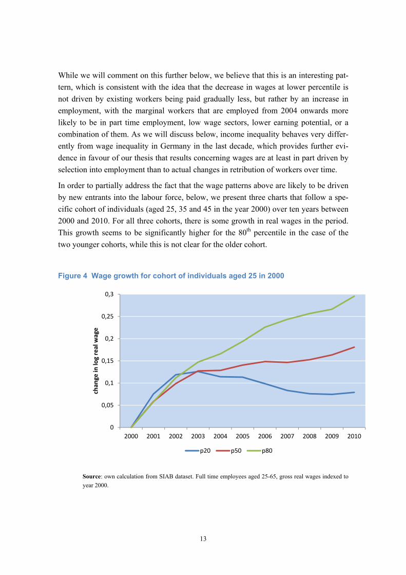
In order to partially address the fact that the wage patterns above are likely to be driven
by new entrants into the labour force, below, we present three charts that follow a spe-
cific cohort of individuals (aged 25, 35 and 45 in the year 2000) over ten years between
2000 and 2010. For all three cohorts, there is some growth in real wages in the period.
This growth seems to be significantly higher for the 80th percentile in the case of the
two younger cohorts, while this is not clear for the older cohort.
Figure 4 Wage growth for cohort of individuals aged 25 in 2000
Source: own calculation from SIAB dataset. Full time employees aged 25-65, gross real wages indexed to
year 2000.
0
0,05
0,1
0,15
0,2
0,25
0,3
2000 2001 2002 2003 2004 2005 2006 2007 2008 2009 2010
chan
ge in
log real wage
p20 p50 p80

14
Figure 5 Wage growth for cohort of individuals aged 35 in 2000
Source: own calculation from SIAB dataset. Full time employees aged 25-65, gross real wages indexed to
year 2000.
Figure 6 Wage growth for cohort of individuals aged 45 in 2000
Source: own calculation from SIAB dataset. Full time employees aged 25-65, gross real wages indexed to
year 2000.
0
0,05
0,1
0,15
0,2
0,25
0,3
2000 2001 2002 2003 2004 2005 2006 2007 2008 2009 2010
chan
ge in
log real wage
p20 p50 p80
0
0,05
0,1
0,15
0,2
0,25
0,3
2000 2001 2002 2003 2004 2005 2006 2007 2008 2009 2010
chan
ge in
log real wage
p20 p50 p80

15
A large part of the fall in real wages at the 20th percentile of the gross wage distribution
is related to new entrants into the labour market during this period of time. This sug-
gests that looking at employed individuals cannot provide a complete picture of inequal-
ity, because it will deliver lower measures of inequality (for the employed) when more
people are unemployed. Next, we move to inequality measures for the working popula-
tion as a whole.

16
4. Inequality among the working age population
By definition, wage inequality concerns workers (and in particular, employees subject
to social security, in the SIAB dataset). However, one may rather be interested in the
trends concerning income inequality at the household level. A recent report by the DIW
(Goebel, Grabka, and Schröder 2015) presents a series of statistics constructed using the
latest version of the SOEP dataset.
If one used only information on employed workers, an important pattern would be miss-
ing. In this sense, it is also important to keep in mind that how one can evaluate differ-
ent policy interventions depends on the goal of those policies. For example, let us con-
sider the introduction of a minimum wage. To the extent that any worker may be paid
less than the minimum wage before its introduction, a minimum wage will bring about
lower inequality among those who work. First of all, because of the increase in the wage
of those directly affected by it, and second, a minimum wage may mean that firms will
have to pay less to higher-wage workers. As a matter of fact, if our only goal was the
Gini coefficient among the employed, we should always want a higher minimum wage.
However, this is not at all the case if our goal is to lower income inequality among all
individuals, including those who do not work. The introduction of the minimum wage
may make it harder for those with skills that are less valuable on the labour market to
start working. But even in the absence of such forces, increasing the income of some
workers may in itself increase income inequality, depending on initial conditions. Re-
form that increase labour market flexibility (which has been argued to have increased in
Germany as a result of the Hartz reforms) may increase wage inequality while decreas-
ing income inequality once we include people who do not work.
The chart below reports Gini coefficients calculated from gross labour income, using
the SOEP dataset. We calculate labour income for employed individuals only (as before,
red line on the chart) as well as for all working-age individuals (blue line). Individuals
who do not work are now coded as having zero labour market income.

17
Figure 7 Inequality in labour income, for employed and for working-age population
Source: own calculations from GSOEP v30, for individuals aged 16-65.
Up until around 2005, the two lines follow similar trends. After 2005, on the other hand,
the Gini coefficient based on labour income that includes all individuals in the working
age population decreases strongly, and after 2008 it is lower than its level in 2000.
These diverging patterns are due to increased labour market participation, which means
that a lower share of the working age population has zero non-labour income. The large
difference between the two lines stresses that labour market participation is extremely
important for labour income inequality among the working-age population. This implies
among other things, that binding minimum wages, while helping some workers, do run
the risk of increasing inequality, once we take non-employed individuals into account.
0,41
0,415
0,42
0,425
0,43
0,435
0,44
0,445
0,45
0,455
0,55
0,555
0,56
0,565
0,57
0,575
0,58
0,585
0,59
0,595
2000 2001 2002 2003 2004 2005 2006 2007 2008 2009 2010 2011 2012
Gini coefficient of the employed
Gini coefficient of all
Labour income of all Labour income of the employed

18
5. Unemployment rates and inequality in the 2000s
The chart below plots the Gini coefficient based upon labour market incomes, which we
calculated for the full population ages 18 - 65. We also plot the unemployment rate in
Germany for the same years. The correlation coefficient is 0.94, which clearly indicates
a strong positive correlation between the two lines. If we believe that inequality in gross
labour income is important, then by far the most important driver of it is the extensive
margin of the labour market. In particular, after 2005 (when the Hartz reforms came in
full effect) as unemployment strongly decreased and more people entered the labour
market, the inequality of before tax labour income decreased strongly as well.
Figure 8 Inequality among the working age population and unemployment
Source: own calculations from SOEP and Destatis data.
We believe that this observation is not only important to understand the development of
inequality among the working-age population as a whole, but also to shed light on the
fact that unemployed individuals are not likely to have average characteristics, similar
to the ones of the working population as a whole. A large increase in employment, such
as the one we observe in Germany between 2005 and 2010, is likely to be largely driven
0,555
0,56
0,565
0,57
0,575
0,58
0,585
0,59
0,595
6
7
8
9
10
11
12
2000 2001 2002 2003 2004 2005 2006 2007 2008 2009 2010 2011 2012
Gini coefficient
Unemploym
ent Rates
Unemployment Rates Gini individual labour income (of all)

19
by individuals who have lower educational attainments compared to the average. This
illustrates a more general point: looking at statistics for employed individuals only may
be misleading if one does not also consider selection into employment, which is typical-
ly such that individuals with higher earning potentials are more likely to be employed.
Respectively, as unemployment rates decrease the pool of the employed becomes more
heterogeneous. This is likely to result in larger heterogeneity in their labour market out-
comes as well.7 Focusing on registered unemployed directly, we present some evidence
from official statistics on unemployment rates by qualification of the workers. The next
two charts look at Eastern Germany and Western Germany separately. In both West and
East Germany, at around 2005 we see a change in the trend by which unemployment
rates decrease overall, and this decrease is disproportionally driven by individuals with
low qualifications leaving unemployment. These are trends that denote an improvement
in labour market opportunities for individuals that have relatively low potential wages
and shows once again that solely looking at wage inequality can be misleading.
Figure 9 Unemployment rates by educational attainment, East Germany
7 Several papers, including M. M. Grabka, Goebel and Schupp (2012), Schmid and Stein (2013) and Adam (2014)
make similar arguments, stressing the importance of strong employment gains since 2006 on the change in the in-creasing trend in income inequality since 2005.
0
10
20
30
40
50
60
2000 2001 2002 2003 2004 2005 2006 2007 2008 2009 2010 2011 2012
Unemploym
ent Rates (percentages)
Overall unemployment rate (East Germany)
Unemployment rate, high school and professional education
Unemployment rate, tertiary education
Unemployment rate, less than high school education

20
Figure 10 Unemployment rates by educational attainment, West Germany
Source: Unemployment rates by qualification, IAB 2013.
0
5
10
15
20
25
30
2000 2001 2002 2003 2004 2005 2006 2007 2008 2009 2010 2011 2012
Unemploym
ent Rates (percentages)
Overall unemployment rate (West Germany)
Unemployment rate, high school and professional education
Unemployment rate, tertiary education
Unemployment rate, less than high school education

21
6. Inequality at the household level
So far, we have focused on inequality across individuals. In fact, much of the literature
on income inequality presents primarily evidence that is calculated at the level of the
households. There are at least two good reasons to focus on households. First, individu-
al incomes are likely to be shared among individuals within the same households, and
decisions are made within the households that affect individual incomes. For example, a
couple may decide for one of them to work part time, and the consequences of that in
terms of individual incomes may not reflect differences in consumption inequality,
which is what we ultimately care about. Secondly, we are interested in investigating the
role of a redistributive welfare state for inequality. In Germany, after tax income con-
cepts only exist at the household level, which is the basic unit for taxation.
Below, we plot Gini coefficients for individual labour income (red line) and for total
household income, both before taxes and transfers. When sharing within the household
is assumed, there is clear evidence that the household provides a strong inequality-
decreasing mechanism: many individuals who have no labour income might live in a
household where others work. This means both that Gini coefficients based on house-
hold labour income are much lower, and also that they are less variable over time. This
is simply because more than one labour income will be combined at the household lev-
el.

22
Figure 11 Inequality in individual and household labour incomes
Source: GSOEP, v30, own calculations for individuals aged 16-65.
There is a large literature showing that sharing within the household in not perfect, in
that sense that who earns a certain income within the household matters for consump-
tion patterns. Even ignoring these considerations and assuming, strongly, that there is
perfect sharing among households’ members and no sharing across households, another
important issue remains: the composition and characteristics of households changes
over time. Peichl, Pestel, and Schneider (2012) investigate exactly this issue, and the
authors state that firm household size plays an important role in the way we can inter-
pret changes in inequality in Germany. Their analysis, which uses data up to 2007,
stresses those changes in household formation. Ignoring taxes and transfers, they find
that as much as 78 percent of the changes in inequality can be explained with changes in
household structure. Because of large redistribution, this share falls to 22 percent if we
consider after tax incomes. Because changes in the distribution and prevalence of
households of different types is part of a long term trend, and at least to some extent
may be related to different choices made by individuals, as pointed out by Sinn (2008),
they should be treated different from changes in inequality that arise from within-group
changes in inequality.
0,38
0,39
0,4
0,41
0,42
0,43
0,44
0,555
0,56
0,565
0,57
0,575
0,58
0,585
0,59
2000 2001 2002 2003 2004 2005 2006 2007 2008 2009 2010 2011 2012
Gini coefficient: Household labour income
Gini coefficient: In
dividual labour income
Individual labour income Household labour income
23
Fessler, Lindner, and Segalla (2014) investigate the role of households’ structure on net
wealth measures across countries, using the HFCS dataset. They find cross country dif-
ferences across households to be important for how we think of relative net wealth lev-
els across countries. What is important to point out is that household size itself may de-
pend on income and wealth, for example to the extent that divorce may be less costly (in
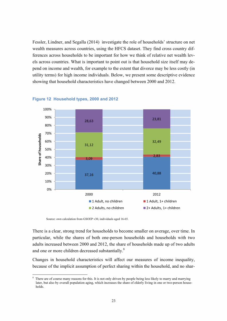
utility terms) for high income individuals. Below, we present some descriptive evidence
showing that household characteristics have changed between 2000 and 2012.
Figure 12 Household types, 2000 and 2012
Source: own calculation from GSOEP v30, individuals aged 16-65.
There is a clear, strong trend for households to become smaller on average, over time. In
particular, while the shares of both one-person households and households with two
adults increased between 2000 and 2012, the share of households made up of two adults
and one or more children decreased substantially.8
Changes in household characteristics will affect our measures of income inequality,
because of the implicit assumption of perfect sharing within the household, and no shar-
8 There are of course many reasons for this. It is not only driven by people being less likely to marry and marrying
later, but also by overall population aging, which increases the share of elderly living in one or two-person house-holds.
37,16 40,88
3,092,83
31,1232,49
28,6323,81
0%
10%
20%
30%
40%
50%
60%
70%
80%
90%
100%
2000 2012
Share of households
1 Adult, no children 1 Adult, 1+ children
2 Adults, no children 2+ Adults, 1+ children

24
ing across households. Using a simple variance decomposition of the same type that we
use in the next section, we find 5.52 percent of the changes in the variance of labour
market incomes at the households level between 2000 and 2012 can be explained by
changes in household size alone.

25
7. Compositional effects: not all inequality is the same
Below, we present evidence of other compositional changes taking place in Germany in
this period. First, we look at changes in characteristics of the working age population
over time. For many of these charts we start in 2003 to stress differences that have taken
place since the first implementation of the Hartz reforms.
Looking at compositional effects is crucial, and it suggests that not all changes in ine-
quality should be treated the same. Some groups of the population (for example, fe-
males, as well as older and more educated workers) tend to have higher wages, but also
higher variance in wage outcomes. If the relative importance of these groups in the la-
bour force increases (as it has been the case in Germany over the last few decades),
overall inequality will increase even when within-group inequality stays the same. Tak-
ing the overall differences as a guidance for policy interventions would be ill-informed
unless one distinguishes between increased inequality between very similar workers
(effects on returns), and increases in the size of groups that tend to have higher variance
from the start (compositional effects). And we believe this is because one should distin-
guish between the fact that some college graduates are paid much more than others
(within group inequality) from the fact that more people are acquiring a college educa-
tion (which increases overall inequality through compositional effects, but may be a
good thing otherwise).
We are not the first to point out that compositional effects may be important for the dy-
namics of inequality in Germany. Klemm and Weigert (2014) look further back to the
mid-1990s and use data from the GSOEP to investigate the importance of compositional
changes for wage inequality. Looking at compositional effects stemming from changes
in labour market experience and education levels, they estimate that around one fourth
of the changes in aggregate wage inequality can be explained by compositional effects.
Given that most of the increase in overall wage inequality took place in the 1990s, it is
likely that the share of increase in wage inequality that can be explained by composition
effects is larger in the last decade. While the public discussion typically focuses on an
aggregate level of inequality, whether and what policy interventions may be a sensible
response to the observed patterns deserves a more sophisticated look at the forces at
work. The part of the rise in wage inequality that is driven by the fact that we live in a
society where people live and work longer, are more likely to be well educated, and
where women participate more in economic activities, should not trigger the same poli-
cy interventions that may be a sensible reaction to increases in wage inequality that is
related to higher returns to unobservable skills in the labour market.

26
The next chart plots full time and part time shares among individuals aged 25-65. While
both full time and part time shares increased substantially between 2003 and 2013, the
share of individuals not working decreased substantially.
Figure 13 Part time and full time employment, 2003 and 2013
Source: own calculation from GSOEP v30, individuals aged 25-65.
Below, we construct the equivalent chart for groups based on educational attainments.
Between 2003 and 2013, among 25-65 year olds there is a significant increase of the
share of individuals with more than high school education, and a corresponding de-
crease in both mid and lower educated individuals.
49,45
52,88
25,98
28,47
24,57
18,65
0% 10% 20% 30% 40% 50% 60% 70% 80% 90% 100%
2003
2013
Full‐Time Part‐Time Not working

27
Figure 14 Educational attainments among 25-65 year olds, 2003 and 2013
Source: own calculation from GSOEP v30, individuals aged 25-65.
The age structure of the population also changed within the same time period, as we
show in the chart below. While the share of individuals aged 25-34 changed relatively
little between 2003 and 2013, the share of people older than 50 increased substantially,
while the share of 35-49 year olds (among 25-65) fell correspondingly.
15,01
14,04
64,16
62,1
20,82
23,86
0% 10% 20% 30% 40% 50% 60% 70% 80% 90% 100%
2003
2013
Less than high school High School More than high school

28
Figure 15 Relative importance of different age groups, 2000 and 2013
Source: own calculation from GSOEP v30, individuals aged 25-65.
Changes in employment rates and full time/part time status that we just discussed are
driven by entry into the labour market of individuals who would otherwise be unem-
ployed. In addition, they are affected by retirement decision. To the extent that older
workers have more heterogeneous wages, this is also going to affect our inequality
measures. The chart below plots effective retirement age for men and women in Germa-
ny between 2000 and 2014.9
9 The average effective age of retirement is calculated as a weighted average of (net) withdrawals from the labour
market at different ages over a 5-year period for workers initially aged 40 and over. In order to abstract from com-positional effects in the age structure of the population, labour force withdrawals are estimated based on changes in labour force participation rates rather than labour force levels. These changes are calculated for each (synthetic) cohort divided into 5-year age groups.
21,93
23,34
44,19
39,47
33,88
37,19
0% 10% 20% 30% 40% 50% 60% 70% 80% 90% 100%
2003
2013
Up to 34 years old 35‐49 years old 50 years old and above

29
Figure 16 Average effective age of retirement in Germany 2000-2014
Source: OECD Ageing and Employment Policies data based on the results of national labour force surveys, the European Union
Labour Force Survey and, for earlier years in some countries, national censuses.
Between 2000 and 2014 there has been a steady increase (with the exception of a drop
due to early retirement programs during the early days of the Great Recession) in the
average effective retirement age in Germany.10 Within this time period, there has also
been a full absorption of the gender gap in retirement age: while in 2000 average effec-
tive retirement age in Germany is equal to 61.0 years of age for men and 60.3 for wom-
en, in 2014 it lies at 62.7 for both men and women. While we will try to identify com-
positional effects in more details in the next sections, these descriptions alone suggest
that delayed retirement is something that one should keep in mind when analysing in-
creased wage inequality, since heterogeneity in labour market compensation tends to be
increasing in age. Older retirement age is also an example of a pattern that may increase
our measures of inequality, but in light of aging populations, it is hardly a negative de-
10 In levels, Germany is among the OECD countries with the highest employment rates among individuals aged 55-
64, at 66.3 percent in 2015. OECD data show that within the European Union only Sweden has higher employment rates among people of that group (74.4 percent). The OECD average lags far behind at 58.2 percent.
60
60,5
61
61,5
62
62,5
63
2000 2001 2002 2003 2004 2005 2006 2007 2008 2009 2010 2011 2012 2013 2014
Men Women
30
velopment. Next, we look at the role of changes in the composition of the population of
employed individuals only. For this, we go back to the SIAB dataset, which allows us to
work with much larger sample size, more precise wage measures and a richer set of con-
trols. Below, we present descriptive statistics from SIAB on full time workers in years
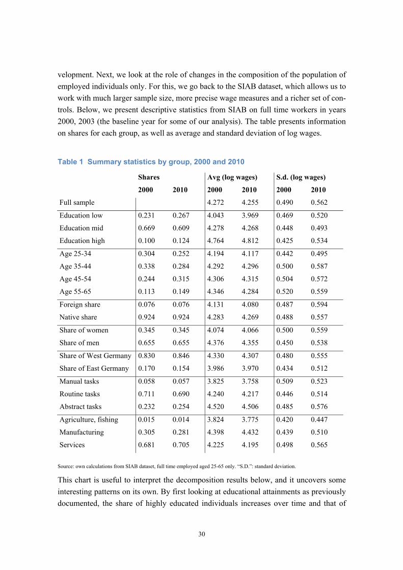
2000, 2003 (the baseline year for some of our analysis). The table presents information
on shares for each group, as well as average and standard deviation of log wages.
Table 1 Summary statistics by group, 2000 and 2010
Shares Avg (log wages) S.d. (log wages)
2000 2010 2000 2010 2000 2010
Full sample 4.272 4.255 0.490 0.562
Education low 0.231 0.267 4.043 3.969 0.469 0.520
Education mid 0.669 0.609 4.278 4.268 0.448 0.493
Education high 0.100 0.124 4.764 4.812 0.425 0.534
Age 25-34 0.304 0.252 4.194 4.117 0.442 0.495
Age 35-44 0.338 0.284 4.292 4.296 0.500 0.587
Age 45-54 0.244 0.315 4.306 4.315 0.504 0.572
Age 55-65 0.113 0.149 4.346 4.284 0.520 0.559
Foreign share 0.076 0.076 4.131 4.080 0.487 0.594
Native share 0.924 0.924 4.283 4.269 0.488 0.557
Share of women 0.345 0.345 4.074 4.066 0.500 0.559
Share of men 0.655 0.655 4.376 4.355 0.450 0.538
Share of West Germany 0.830 0.846 4.330 4.307 0.480 0.555
Share of East Germany 0.170 0.154 3.986 3.970 0.434 0.512
Manual tasks 0.058 0.057 3.825 3.758 0.509 0.523
Routine tasks 0.711 0.690 4.240 4.217 0.446 0.514
Abstract tasks 0.232 0.254 4.520 4.506 0.485 0.576
Agriculture, fishing 0.015 0.014 3.824 3.775 0.420 0.447
Manufacturing 0.305 0.281 4.398 4.432 0.439 0.510
Services 0.681 0.705 4.225 4.195 0.498 0.565
Source: own calculations from SIAB dataset, full time employed aged 25-65 only. “S.D.”: standard deviation.
This chart is useful to interpret the decomposition results below, and it uncovers some
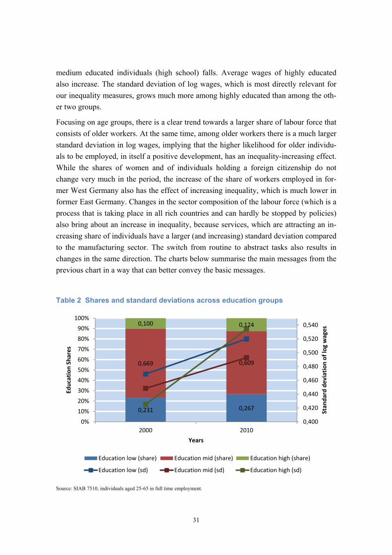
interesting patterns on its own. By first looking at educational attainments as previously
documented, the share of highly educated individuals increases over time and that of
31
medium educated individuals (high school) falls. Average wages of highly educated
also increase. The standard deviation of log wages, which is most directly relevant for
our inequality measures, grows much more among highly educated than among the oth-
er two groups.
Focusing on age groups, there is a clear trend towards a larger share of labour force that
consists of older workers. At the same time, among older workers there is a much larger
standard deviation in log wages, implying that the higher likelihood for older individu-
als to be employed, in itself a positive development, has an inequality-increasing effect.
While the shares of women and of individuals holding a foreign citizenship do not
change very much in the period, the increase of the share of workers employed in for-
mer West Germany also has the effect of increasing inequality, which is much lower in
former East Germany. Changes in the sector composition of the labour force (which is a
process that is taking place in all rich countries and can hardly be stopped by policies)
also bring about an increase in inequality, because services, which are attracting an in-
creasing share of individuals have a larger (and increasing) standard deviation compared
to the manufacturing sector. The switch from routine to abstract tasks also results in
changes in the same direction. The charts below summarise the main messages from the
previous chart in a way that can better convey the basic messages.
Table 2 Shares and standard deviations across education groups
Source: SIAB 7510, individuals aged 25-65 in full time employment.
0,231 0,267
0,669 0,609
0,100 0,124
0,400
0,420
0,440
0,460
0,480
0,500
0,520
0,540
0%
10%
20%
30%
40%
50%
60%
70%
80%
90%
100%
2000 2010
Stan
dard deviation of log wages
Education Shares
Years
Education low (share) Education mid (share) Education high (share)
Education low (sd) Education mid (sd) Education high (sd)

32
Table 3 Shares and standard deviations across age groups
Source: SIAB 7510, individuals aged 25-65 in full time employment.
Table 4 Shares and standard deviations across tasks
Source: SIAB 7510, individuals aged 25-65 in full time employment.
0,304 0,252
0,3380,284
0,2440,315
0,113 0,149
0,400
0,450
0,500
0,550
0,600
0%
10%
20%
30%
40%
50%
60%
70%
80%
90%
100%
2000 2010
Stan
dard deviations of log wages
Age
group shares
Years
Age 25‐34 (share) Age 35‐44 (share) Age 45‐54 (share)
Age 55‐65 (share) Age 25‐34 (sd) Age 35‐44 (sd)
Age 45‐54 (sd) Age 55‐65 (sd)
0,058 0,057
0,711 0,690
0,232 0,254
0,440
0,460
0,480
0,500
0,520
0,540
0,560
0,580
0%
10%
20%
30%
40%
50%
60%
70%
80%
90%
100%
2000 2010
Stan
dard deviation of log wages
Task Shares
Years
Manual Task (share) Routine Tasks (share) Abstract Tasks (share)
Manual Task (sd) Routine Tasks (sd) Abstract Tasks (sd)

33
Table 5 Shares and standard deviations across sectors
Source: SIAB 7510, individuals aged 25-65 in full time employment.
The main decomposition exercise that we perform is based on a so called recentered
influence function (RIF) regression approach which was introduced by Firpo, Fortin,
and Lemieux (2009). This decomposition method is based on linear regressions and
allows us to quantify the relative importance of single variables on the change in wage
inequality, which we measure by the change in the variance of log real wages over time.
This implies that we are able to look at the effect of a single characteristic, while hold-
ing the other variables constant. Moreover we are able to distinguish between so called
composition and wage structure effects to the rise in wage inequality. Composition ef-
fects are linked to changes in the underlying distribution of covariates in the population
over time. Think for example of shifts in the age-profile of the workforce. As mentioned
earlier, we observe a shift towards older workers. Even if there were no changes in re-
turns to age, we could observe an increase in wage inequality simply because the group
of older workers shows a relatively high within-group wage inequality. Wage structure
effects, on the other hand, are linked to changes in the returns to single characteristics
and also capture changes in within group wages. Coming back to our example, we could
also observe an increase in wage inequality if returns to age (or experience) change over
time, even if the distribution of age groups remains constant. Formally, a recentered
influence function regression for period t can be expressed as follows
0,015 0,014
0,305 0,281
0,681 0,705
0,420
0,440
0,460
0,480
0,500
0,520
0,540
0,560
0%
10%
20%
30%
40%
50%
60%
70%
80%
90%
100%
2000 2010
Stan
dard deviation of log wages
Sector Shares
Years
Agriculture (share) Manufacturing (share) Services (share)
Agriculture (sd) Manufacturing (sd) Services (sd)

34
,
where is the recentered influence function of the variance of real log wages,
is a vector of the covariates and is the corresponding vector of parameters. is a
standard error term. Based on the regression results we can then perform a decomposi-
tion of the variance of real log wages between two different time periods (t=0 and t=1),
which can be formalised as
∆ ,
where the first term on the right-hand side denotes the wage structure effect and the
second tern denotes the composition effect.
Before we come to the results of this RIF-regression approach, we go one step back and
discuss the results of a much simpler exercise, where we investigate, for one variable at
a time, the role of compositional effects on the difference in wage inequality (which we
measure here with the variance in log wages). In particular, we use the following formu-
la to decompose the pooled variance into groups. In this example, we write the formula
for two groups for simplicity. Let the two groups be identified by 1 and 2. The corre-
sponding means and standard deviations are denoted by , , and . The number
of observations of the first and of the second group are and respectively. The var-
iables without subscripts refer to the full sample. We can write the variance of the full
sample at a certain moment in time as 1
12 μ12
222 μ22 2
We calculate the overall variance for each time period we are looking at, and then calcu-
late a counterfactual variance that is obtained by applying the shares of the second peri-
od while using means and standard deviations of the first period. This exercise will help
us isolate the effect of changes in the relative size of the groups.
35
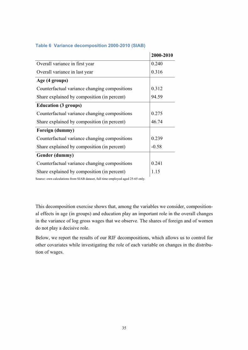
Table 6 Variance decomposition 2000-2010 (SIAB)
2000-2010
Overall variance in first year 0.240
Overall variance in last year 0.316
Age (4 groups)
Counterfactual variance changing compositions 0.312
Share explained by composition (in percent) 94.59
Education (3 groups)
Counterfactual variance changing compositions 0.275
Share explained by composition (in percent) 46.74
Foreign (dummy)
Counterfactual variance changing compositions 0.239
Share explained by composition (in percent) -0.58
Gender (dummy)
Counterfactual variance changing compositions 0.241
Share explained by composition (in percent) 1.15 Source: own calculations from SIAB dataset, full time employed aged 25-65 only.
This decomposition exercise shows that, among the variables we consider, composition-
al effects in age (in groups) and education play an important role in the overall changes
in the variance of log gross wages that we observe. The shares of foreign and of women
do not play a decisive role.
Below, we report the results of our RIF decompositions, which allows us to control for
other covariates while investigating the role of each variable on changes in the distribu-
tion of wages.

36
Table 7 Recentered Influence Function Decomposition
2000-2010
Observable difference in vari-ance between t and t+1 7.64
Composition effects
West -0.06
Female 0.00
Tasks 0.16
Education 0.65
Age 0.48
Foreign 0.00
Sector 0.48
Total 1.71
Wage structure effects
West -1.48
Female -0.56
Tasks 0.62
Education 2.65
Age -1.98
Foreign 0.30
Sector -1.28
Constant 7.88
Total 6.15
Source: SIAB 7510 dataset, fulltime workers aged 25-65.
Notes:
Variables west, female, foreign are dummy variables; base group is equal to dummy=0; for all other categorical variables the base
group refers to the median group (education: low, medium, high -> base group: medium, age: 25-34, 35-44, 45-54, 55-65 -> base
group: 35-44; tasks: manual, routine, abstract -> base group : routine; sector: includes 17 categories ->base group is group "manufac-
turing"); The wage structure effects depend on the definition of the base group. The methodology used here is described in detail in
Firpo, Fortin, and Lemieux (2009). All coefficients above are multiplied by 100 for convenience. Reweighting error: -0.04, specifica-
tion error: -0.18.
The table above shows the results of the RIF-decomposition for changes in the variance
of real log wages between 2000 and 2010, numbers are multiplied with 100 to represent

37
(variance) log points. Around one fifth of the overall change in the variance of log real
wages can be explained by changes in the composition of the population. Education,
industry (with the well documented move towards services) and age groups are the most
important variables through which compositional effects operate. To a smaller extend
also changes in the task structure of the population (a movement towards a higher share
of abstract tasks and a lower share of routine tasks) have an inequality increasing im-
pact.
The total wage structure effect captures the impact of changes in returns to characteris-
tics and changes in within group wage inequality. It accounts from around 80 percent of
the observed overall change in wage dispersion. We find a strong inequality increasing
wage structure effect for our education variable, this captures on the one hand the in-
crease in the high-skilled wage premium (unconditional log mean wages for high skilled
workers increase from 4.76 in 2000 to 4.81 in 2010, while the return to skill for medium
skilled workers, the base group, declined from 4.28 to 4.27 over the same time period).
On the other hand this effect also captures the strong increase in within-group wage
inequality for low and high educated workers, relative to medium skilled workers. Ine-
quality increasing wage structure effects are also found for the tasks and foreign varia-
ble, although the magnitude is much smaller. At the same time we find inequality reduc-
ing wage structure effects for the variables age, west, sector and female. Taking the age
effect as an example this again reflects a direct effect of changes in returns to age (or
experience) and changes in within group wage dispersion. More specifically it captures
that the returns to age decreased in most age groups relative to the base group (which is
the 35-44 year olds) and that within group wage inequality increased less in all age
groups relative to the base group.
Overall the results suggest that a non-negligible part of the observable increase in wage
dispersion (about one fifth) is driven by compositional changes in the labour force. This
has to be kept in mind when thinking about policy responses to the increase in inequali-
ty. This means that a relatively large extent the changes in the overall inequality are
driven by changes in the composition of the labour force and in the types of jobs that
prevail in the economy. These changes call for a different (if any) policy response to the
changes in inequality within narrowly defined groups of workers.

38
8. Taxation and net inequality
So far, all of the inequality concepts we described relate to before tax incomes. Howev-
er, it is important to investigate the effect of the existence of taxation for inequality.
Because taxes are calculated at the level of the household in Germany, when looking at
inequality in after tax income we need to look at total household income. Below, we
plot Gini coefficients based on household incomes before and after taxes.
Figure 17 Inequality of household income before and after taxes
Source: GSOEP, v30, own calculations for individuals aged 16-65.
The red line depicts the Gini coefficient of market income. Since 2005, we clearly ob-
serve a decrease in the market Gini coefficient (right axis) until 2010, followed by a
moderate increase. The decrease in the Gini coefficient is much larger when we look at
before tax incomes than when we look at net incomes. The two trends combined are
consistent with the idea that after 2005 the increased employment rates in Germany
have meant that more people entered the labour market.
The market incomes of the households of these marginal entrants are affected much
more than their after tax incomes, because of the presence of a redistributive welfare
state. In other words, before 2005 after tax incomes for those families without (or with a
0,25
0,26
0,27
0,28
0,29
0,3
0,385
0,39
0,395
0,4
0,405
0,41
0,415
0,42
2000 2001 2002 2003 2004 2005 2006 2007 2008 2009 2010 2011 2012
After Taxes
Before Taxes
Before Taxes After Taxes

39
low) labour income could stay relatively high, while their market incomes were very
low. After 2005, many of the individuals in these households entered the labour market,
which boosted their total before tax income, while the changes in after tax incomes were
more moderate.

40
9. Germany and other OECD countries
In the previous section, we have introduced taxation into our analysis, and looked at its
effects on income inequality. We now evaluate the size and type of redistribution on
Germany, compared to similar countries. First, we look at after tax income inequality
across selected OECD countries. The figure below reports values of the Gini coefficient
in the OECD countries where such comparable data exists, calculated using household
disposable income in 2012 (and in 1995, for comparison). The increase in income ine-
quality of the 1990s and early 2000s in Germany resulted in the leaving of the group of
countries with the lowest levels of income inequality. The levels of the Gini coefficient
in Germany are now closest to those of the Netherlands and France, lower than those of
Southern Europe and of the Anglo Saxon countries.
Figure 18 Gini coefficient, selected OECD countries
Source: OECD Income Distribution Database. Gini coefficients calculated for household disposable income. For some of the coun-tries, we need to use previous or following years because of data limitations.
Beyond looking at the level of the after-tax Gini coefficient across countries, it is also
informative to compare it to the Gini coefficient calculated on market income. The table
0,2
0,22
0,24
0,26
0,28
0,3
0,32
0,34
0,36
0,38
0,4
2012 1995

41
below lists a group of selected countries (that are relatively large, rich, and with rela-
tively large governments) by their Gini coefficient calculated from market income as
well as from net income. Perhaps surprisingly, Germany is close to the bottom of the
chart. Based on market income Germany has much higher levels of inequality compared
to similar countries. In particular, it records a Gini coefficient from market income
higher than Austria, France, Italy as well as the United Kingdom and the United States.
Figure 19 Before and after tax Gini coefficients, sorted by market income
Because of the redistributive role of the government, which is substantial in many of
these countries, the Gini coefficient based on net income is lower than that calculated
from market incomes. Addressing this endogeneity directly is beyond the scope of this
report, but it is interesting to note that there are reasons to believe that Gini calculated
on market incomes is at least in part itself a response to the activities of the government.
For example, a German firm that wants to hire a electronical engineers needs to offer
her a take-home pay that is competitive with that of other countries. In Germany, this
implies a higher gross pay than in the US or the UK, because of higher taxes. This
underlines a mechanism that may actually limit the full effect of redistributive policies.
0 10 20 30 40 50
BrazilSweden
GermanyDenmark
United KingdomItaly
United StatesFinland
IsraelFrance
AustraliaTurkeyAustria
CanadaSpain
SwitzerlandNew ZealandNetherlands
NorwayJapan
Source: SWIID dataset and IMF World Economic Outlook data, 2012
Market income Net income

42
If more mobile factors of production face higher taxes, firms may choose to pay other
factors of production less in order to offer competitive compensation packges to the
employees they are more at risk of losing. Below, we show the Gini coefficients from
market and net income again, this time sorting countries based on their Gini calculated
from net income, i.e. after taxes and transfers are taken into account.
Figure 20 Before and after tax Gini coefficients, sorted by net income
Now, Germany is close to the top of the chart, with inequality levels similar to the
Nordic countries, and smaller than any other large OECD economy, most notably
smaller than France, Spain, Italy, the United Kingdom and the United States. It is worth
noting that this is not the case for all countries. In other words, it is not the case that all
countries with high market Gini redistribute a lot (which is what a simple median-voter
model would predict). For example, Brazil, Turkey and the United States redistribute
relatively little, albeit starting from relatively high inequality levels.
0 10 20 30 40 50
BrazilTurkey
IsraelUnited States
United KingdomSpain
AustraliaItaly
New ZealandCanadaFrance
SwitzerlandJapan
GermanyAustria
NetherlandsDenmarkSwedenFinlandNorway
Source: SWIID dataset and IMF World Economic Outlook data, 2012
Market income Net income

43
These charts show that the redistribution system in Germany plays a decisive role in
shaping the level of net income inequality that we observe. Germany redistributes more
than almost all other OECD countries (Fuest 2016). In the simplest specification of a
government budget constraint, the government is typically assumed to only redistribute
from richer to poorer households, for example with a per-capita transfer and proportion-
al taxation. Redistribution from top to bottom clearly can impact after tax inequality. It
comes at a price, however, in the sense that increasing the extent to which income is
redistributed is likely to negatively impact economic growth, and this effect is likely to
be rising at an increasing rate. The efficiency costs of redistribution, especially in coun-
tries such as Germany where levels are already quite high, should be part of the debate
on inequality, especially in a global context where future sustainability of the welfare
state is challenged from many directions. Next, we construct some simple and rough
measures of the extent to which large governments redistribute more.

44
10. Relative efficiency of government redistribution
Typically, we think of the government redistribution exclusively as a movement of re-
sources from the top to the bottom of the income distribution. In reality, the role of gov-
ernments in the economy is more complex. We look at the relationship between the size
of the government and the difference between inequality before and after taxes and
transfers. In the next chart, we measure the size of the government with general gov-
ernment expenditures as share of GDP (on the horizontal axis) and the extent of redis-
tribution with the ratio between the Gini coefficient measured after taxes and transfer
and the Gini coefficient before taxes (a large ration means less redistribution).
Figure 21 Size of government and redistribution
The countries that are on the right in the chart have large governments, while those that
are higher on the chart are those with less redistribution. Comparing countries along the
vertical axis shows that Germany redistributes a lot, with only the Nordic countries re-
distributing more. However, comparing countries horizontally shows that Germany,
Argentina
Australia
Austria
Belgium
Brazil
Canada
Czech Republic
Denmark
Egypt
Finland
France
Germany
Greece
Hungary
Ireland
Israel
Italy
Japan
Netherlands
New Zealand
Norway
Poland
Portugal
Romania
Russian Federation
South Africa
Spain
Sweden
Switzerland
Turkey
Ukraine
United Kingdom
United States
VenezuelaVietnam
= -0.012R squared = 0.50
.5.6
.7.8
.91
Gin
i afte
r ta
xes
/ Gin
i bef
ore
taxe
s
30 40 50 60General government total expenditures, percent of GDP
Source: SWIID dataset and IMF World Economic Outlook data, 2012

45
while redistributing a lot, has a government that is not as large (as share of GDP) as
many other countries, including Italy, Austria and France. It is worth noting that despite
the fact that we restrict our attention to countries where the government is at least 30
percent of the economy, there are still many countries (including Brazil, Turkey, Argen-
tina and South Africa) that redistribute very little based on the SWIID and IMF data.
The red line on the chart is a linear regression line and shows that there is a relatively
strong negative correlation between the two variables. However, the chart also shows
that many countries (we included only relatively rich countries with a well-working
revenue collection system) are not close to that regression line. Countries to the left of
that line may be described as relatively “efficient” governments (in terms of redistribu-
tion), and Germany is the only large economy in this group. Given its size, the German
government seems to be using relatively many public funds for redistribution.11 Other
countries, such as Greece, Belgium and France, have a large government but relatively
little redistribution (or perhaps more redistribution that does not go from rich to poor,
we are not able to disentangle the two from the chart). This means that their relatively
high levels of taxation do not translate into a decrease in after tax inequality. In this
sense, the discussion in Economist (2014) may be simplistic, since it implies that size of
government and extent of redistribution are the same concepts. For many of the mecha-
nisms through which the role of the government might affect growth, the channel might
not be uniquely redistribution, but rather the size of the government in the economy. For
example, when the government is a very large employer and pays higher wages than the
market, this will make it hard for businesses to find the type of workers they are looking
for.
The importance of the government in the economy matters for international competi-
tiveness as well, since higher tax rates are likely to reduce competitiveness. This again
suggests that assuming that a large government automatically provides more generous
social programs and redistribution to the poor may be incorrect and potentially mislead-
ing. Moving towards a simplified tax system may increase the extent of redistribution,
limit horizontal inequity and also increase transparency, which is of great importance in
a context there currently a large share of individuals feel that they are getting too little
and paying too much. So far, our analysis shows that the net income inequality in Ger-
many is not higher than in many other countries, but is higher than in the early 1990s. It
does seem, however, that a relatively large section of the German electorate would like
to see inequality fall further. It is not our role as researchers to make normative state-
11 A word of caution is necessary here: taxes and transfers are not the only way for a government to redistribute con-
sumption/utility across individuals. The provision of public goods including education, health and infrastructure has a redistributive component as well, which is not captured in these charts.
46
ments on whether the Gini should rise or fall. Rather, we would like to comment on
different policy recommendations and what their effects on income inequality may be.
Further increasing redistribution, for example increasing top marginal tax rates, would
probably reach the desired goals. But this might not come at low costs, given the fact
that at higher levels of taxation may negatively affect growth.
From the two tables above, it seems relatively clear that the level of inequality in ‘not
incomes’ in Germany stems, to a very large extent, not from lack of redistribution by
the welfare state (which is actually among the most substantial worldwide) but rather
from a large level of before-tax income inequality. We believe that market income ine-
quality can also be affected by policy. However, we also claim that those are quite dif-
ferent from the policies that are most often suggested, which usually focus on the tax
and transfer system. The distribution of non-market income, on the other hand, has little
to do with taxation, and is arguably harder to tackle. While difficult, however, we be-
lieve that it warrants further attention. Focusing on pre-tax distribution of incomes may
allow to avoid the usual tradeoff between redistribution and growth (whose effects are
depicted in the Laffer curve), which one needs to face when addressing inequality only
from the perspective of redistribution, implicitly taking pre-tax incomes as given.
On the contrary, one can envision policies that can move out this tradeoff, lowering ine-
quality without affecting (or potentially boosting) overall economic growth. Some of the
directions for policies discussed below are also discussed in Keuschnigg (2015). The
risks of the current inequality debate is that it very narrowly focuses on policies that
may affect net inequality in the short term (without affecting before-tax inequality) and
may thereby decrease our attention to other policy areas, which might be very im-
portant. Moreover, the current debate sometimes forgets that a decrease in inequality is
hardly a goal in itself.
Sectors with high levels of innovation are likely to generate employment, but to the ex-
tent that they are particularly successful, may also generate new riches. These, do not
need to be detrimental to society’s welfare if individual skills are used efficiently. On
the other hand, when wealth is generated by previous wealth, and perhaps accumulated
in the form of rents from unproductive assets or activities without sufficient market
competition, effects on poverty and welfare will not be the same. It is therefore clear
that competition and efficiency should directly be regarded in this larger debate, with
the goal of keeping the debate pragmatic and not biased by ideology.
In order to evaluate the extent to which the redistribution that we have discussed is
achieved through very high taxes on individuals with large incomes, we next plot a

47
chart that has the same vertical axis as the previous chart, with the highest marginal tax
rate on the horizontal axis.
Figure 22 Highest marginal tax rate and redistribution
Countries on the right of the above chart are those with the highest marginal tax rates
for high-income individuals. Germany’s top marginal tax rate is similar to that of Italy
and Canada, and only slightly higher than that of the US and the UK. At the same time,
Germany is plotted lower on the chart, meaning that with a similar tax rate it seems to
achieve more redistribution. Among large European economies, Germany is the only
country that is relatively far below the regression line in that chart, while Spain and
France, among others, are above the line, with relatively high top tax rates but less re-
distribution than Germany.
Australia
Austria
BelgiumCanada
Chile
DenmarkFinland
France
Germany
Italy
Japan
Mexico
Netherlands
Norway
Portugal
Spain
Sweden
Switzerland
Turkey
United Kingdom
United States
= -1.210
R squared = 0.49
.5.6
.7.8
.91
Gin
i afte
r ta
xes
/ Gin
i bef
ore
taxe
s
.3 .4 .5 .6Highest marginal tax rate (2012)
Source: SWIID dataset and OECD Tax Database. Selected OECD countries, 2012

48
11. The role of public goods
The previous section pointed out that the government acts as a redistributor of income
between different segments of society. This is not the only activity modern governments
engage in. In particular, in Germany and elsewhere, the government provides some pub-
lic goods to the population. To the extent that the financing or the utilization of these
public goods differs across individuals, public goods provisions have distributive ef-
fects. This also implies that looking at the income Gini coefficient alone can be mislead-
ing for policy advice, since it ignores that there may be policies that redistribute in kind
and that may be more efficient than others in achieving lower consumption inequality,
which is in the end what matters the most.
For example, in Germany public health insurance is paid as a percentage of labour in-
come. Therefore, individuals with larger incomes pay more into the system, and may get
the same (or less, to the extent that richer individuals are healthier) services, which im-
plies that the system is progressive in nature. Whilst progressive, it does not typically
get counted for inequality measures since services are provided in kind rather than in
cash. Using data from the World Bank’s World Development Indicators (WDI), it is
clear that many of the public goods that are provided by the government in Germany
have a redistributive nature. The two most prominent examples are government expend-
itures for health and education.12 According to the WDI data, Germany spends 19.42
percent of all government expenditures on health (data from 2013) and 11.03 percent on
education (data from 2011).13 Even if we focus on health and education only, we can
conservatively estimate the yearly per capita expenditures by the government for health
and education to be around 3,750 Euros (in 2012). If we view these expenditures as a
demogrant (which is certainly not the case in a static sense, but it is not a bad approxi-
mation of the actual expenses that individuals would have were the government to step
back) and were to calculate the Gini coefficient on net incomes again including these
expenditures, the overall Gini coefficient in Germany on net income would decrease
12 According to data from DeStatis, in Germany overall expenditures on education are around 4.1percent of GDP,
which is actually lower than public expenditures as a share of GDO according to the OECD data. This is clearly a data inconsistency, probably due to the fact that education expenditures pertain to different levels of government, and are therefore not easy to calculate. Nevertheless, it underlines that the vast majority of expenditures on educa-tion is borne by the government (and therefore the tax payer). There are clear differences between Germany and other OECD countries such as the UK and the US in this respect, which have an effect on inequality although they are not going to be included in the way we typically calculate inequality.
13 These values are significantly higher than those for the Euro Area as a whole, and of the OECD as a whole. Private health expenditures, on the other hand, in Germany are just over 55 percent of OECD average in Germany (as share of GDP), which suggests that if public expenditures were to be cut, private expenditures would have to in-crease, which would of course hurt relatively poor households more. And they are substantial amounts for the me-dian family. The Germany statistical agency estimated the costs to the state of each student up to university (master level) to be around 143,000 Euros (Statistisches Bundesamt 2015).
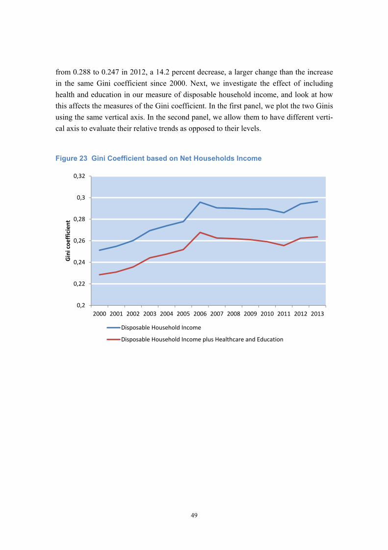
49
from 0.288 to 0.247 in 2012, a 14.2 percent decrease, a larger change than the increase
in the same Gini coefficient since 2000. Next, we investigate the effect of including
health and education in our measure of disposable household income, and look at how
this affects the measures of the Gini coefficient. In the first panel, we plot the two Ginis
using the same vertical axis. In the second panel, we allow them to have different verti-
cal axis to evaluate their relative trends as opposed to their levels.
Figure 23 Gini Coefficient based on Net Households Income
0,2
0,22
0,24
0,26
0,28
0,3
0,32
2000 2001 2002 2003 2004 2005 2006 2007 2008 2009 2010 2011 2012 2013
Gini coefficient
Disposable Household Income
Disposable Household Income plus Healthcare and Education

50
Source: World Bank World Development Indicators, SOEP v30.
Gini coefficients based on after-tax household are much lower than Gini’s that excludes
them. The Gini coefficient that includes health and education decreases somewhat more
after 2005/2006, compared to the Gini that excludes them. This reflects an increase in
the government expenditures in health and education as a share of per capita income in
this period.
In reality, expenditures on health and education do not benefit each individual and each
household in the same way. For example, in a cross sectional sense, health expenditures
are disproportionally going towards the old and the poor (who are more likely to have
poorer health), and expenditures on higher education are more likely to favour relatively
rich families, who are more likely to send their kids to university in Germany, with
higher coefficients of intergenerational transmission of educational attainments failing
to decrease despite massive interventions, as discussed in Heineck and Riphahn (2009).
In a static sense, this means that we are ignoring the provision of public goods across
different groups in the population, and the fact that consumption inequality may be dif-
ferent for two countries that have the same level of income inequality because of this, in
the case in which some goods or services are provided by the government directly only
in one of those countries. This matters dynamically as well, in the sense that changes in
public goods provisions, which are very likely to affect consumption inequality in reali-
0,225
0,23
0,235
0,24
0,245
0,25
0,255
0,26
0,265
0,27
0,25
0,26
0,27
0,28
0,29
0,3
2000 2001 2002 2003 2004 2005 2006 2007 2008 2009 2010 2011 2012 2013
Gini coefficient (including health and education)
Gini coefficient
Disposable Household Income
Disposable Household Income plus Healthcare and Education

51
ty, is something that we would not notice in the inequality statistics that we typically
use. We are not pointing out these issues as an intellectual exercise, but because we be-
lieve that they matter greatly in the public discourse. In particular, we believe that a
narrow focus on decreasing income inequality though redistributive monetary transfers
runs the risk of ignoring the issues around public goods, as well as equality of opportu-
nities and economic incentives, which are likely to be crucial for future prosperity, as
well as for future inequality.

52
12. Wealth inequality and measurement issues
While most economists agree that the ultimate objective would be to analyse consump-
tion inequality, the debate around inequality focuses primarily on income inequality.
The reason for this is primarily that income can be more readily and relatively precisely
measured. From the perspective of economic theory, our focus should actually be on
wealth, since forward-looking individuals will decide their consumption paths based on
their level of lifetime wealth. Wealth is however rather difficult to measure. Recently,
however, there are some attempts at measuring it, thereby offering some indications
about wealth inequality in Germany.
Fuchs-Schuendeln, Krueger, and Sommer (2010) use data from the Income and Ex-
penditure Survey (EVS), which is a cross sectional dataset carried out every five years,
to get information on consumption and wealth (until 2003).
Even more recently, Grabka and Westermeier (2014) use SOEP data to describe recent
wealth inequality in Germany.14 While it is very hard to compare countries in this re-
spect given that wealth data is collected differently, they argue that Germany has high
levels of wealth inequality compared to many other countries in Europe. In particular,
they find a Gini coefficient of around 0.78 in 2012. Around 28 percent of respondents
report zero or negative wealth. In addition, they report large differences between West
and East Germany. A discussion of recent trends in wealth inequality in Germany is
also available in Grabka (2015). Grabka and Westermeier (2014) use data from the
GSOEP to investigate the distribution of wealth across German households. They find
that over half of the households report either zero or slightly negative wealth. They then
find the 75th percentile of the net wealth distribution to be around 100,000 Euros (of
year 2011), the 90th percentile to be around 200,000 Euros and the 95th percentile
around 300,000 Euros.
We believe that what we can learn from the SOEP about wealth inequality in Germany
is limited. First, findings from the SOEP seem to have an excessive share of households
with no wealth. It is hard to be convinced that low home ownership rates and the fact
that durables and valuables are excluded (which is by itself problematic) are sufficient
to explain this. Second, the amount of information that is available about the types of
assets and liability that make up the given wealth level is very limited. This means that
with the SOEP we are not going to be able to evaluate how different policy environ-
ments may affect the wealth of different households differently.
14 In the SOEP, there is information on wealth at the individual and at the household level for 2002, 2007 and 2012.

53
We therefore turn to a different dataset: the “Household Finance and Consumption Sur-
vey” (HFCS) dataset.15 Some of the findings from the HFCS dataset are also discussed
in Bundesbank (2013). This dataset (only a cross section at this stage, but that will be
further developed into a panel over time) includes information on assets and liabilities
of households across the Euro area. The sample for Germany, which is the one we use
for our analysis, includes 3565 households (from around 2100 we have full wealth in-
formation), with data collected in 2010-2011. The dataset is prepared using multiple
imputations to address the issue of non-random non-response, which is large in this con-
text.
Using a weighted multiple imputation procedure, we find that the overall average
household wealth is around 195,000 Euros, the 5th percentile of that distribution is
around -1600 Euros, the 10th percentile is very close to zero, the 25th percentile is
around 600 Euros. The median household has a wealth of around 50,000 Euros, while
the 75th percentile has around 200,000 Euros, the 90th percentile 450,000 and the 95th
percentile 650,000 Euros. Because of sample size considerations, we divide our sample
in four groups only, one for each of the four quartiles of the distribution of net wealth.
Below, we show some of the quantiles of the net wealth distribution. For the following
tables, we only divide the sample into four quartiles in order to be able to work with
sufficiently large sample sizes for all of the statistics that we are looking at.
Table 8 The distribution of wealth in the HFCS
Percentiles of the net wealth distribution Net wealth
5th percentile -1616
10th percentile 64
25th percentile 6600
Median 51358
75th percentile 209820
90th percentile 442320
95th percentile 661240
Source: Own calculations from the HFCS dataset.
15 We thank the European Central Bank for allowing us to use this restricted-access dataset.
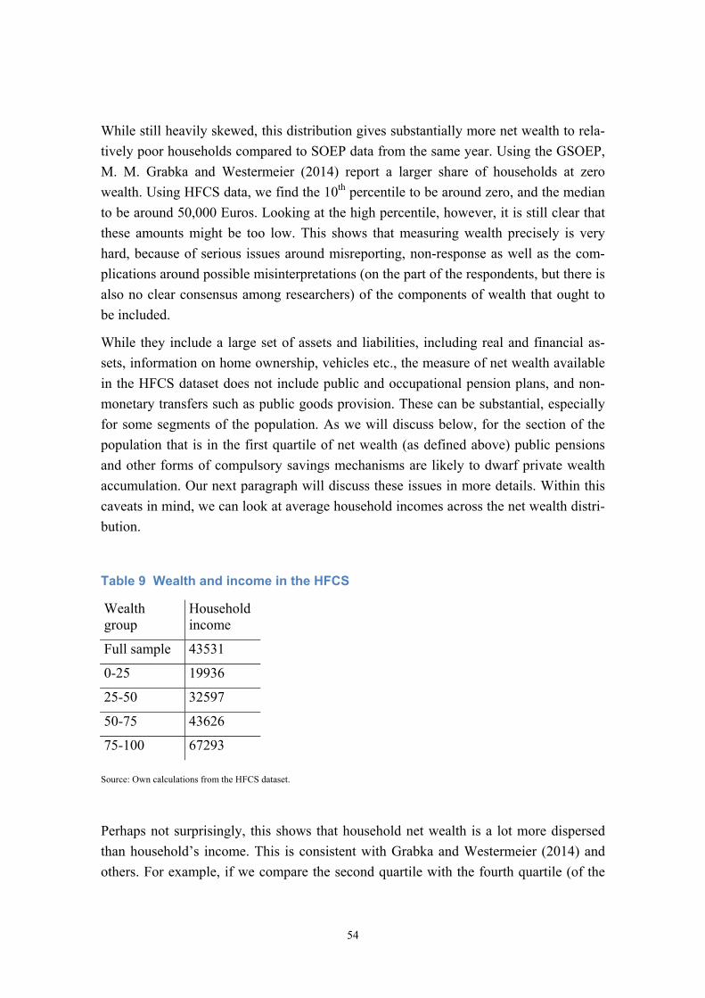
54
While still heavily skewed, this distribution gives substantially more net wealth to rela-
tively poor households compared to SOEP data from the same year. Using the GSOEP,
M. M. Grabka and Westermeier (2014) report a larger share of households at zero
wealth. Using HFCS data, we find the 10th percentile to be around zero, and the median
to be around 50,000 Euros. Looking at the high percentile, however, it is still clear that
these amounts might be too low. This shows that measuring wealth precisely is very
hard, because of serious issues around misreporting, non-response as well as the com-
plications around possible misinterpretations (on the part of the respondents, but there is
also no clear consensus among researchers) of the components of wealth that ought to
be included.
While they include a large set of assets and liabilities, including real and financial as-
sets, information on home ownership, vehicles etc., the measure of net wealth available
in the HFCS dataset does not include public and occupational pension plans, and non-
monetary transfers such as public goods provision. These can be substantial, especially
for some segments of the population. As we will discuss below, for the section of the
population that is in the first quartile of net wealth (as defined above) public pensions
and other forms of compulsory savings mechanisms are likely to dwarf private wealth
accumulation. Our next paragraph will discuss these issues in more details. Within this
caveats in mind, we can look at average household incomes across the net wealth distri-
bution.
Table 9 Wealth and income in the HFCS
Wealth group
Household income
Full sample 43531
0-25 19936
25-50 32597
50-75 43626
75-100 67293
Source: Own calculations from the HFCS dataset.
Perhaps not surprisingly, this shows that household net wealth is a lot more dispersed
than household’s income. This is consistent with Grabka and Westermeier (2014) and
others. For example, if we compare the second quartile with the fourth quartile (of the

55
net wealth distribution) we find that household income is on average about twice as
large, and the net wealth differs by a factor of 20. This of course has to do with the fact
that one is a flow variable and one is a stock that accumulated over time, and also with
the fact that different households might be in a different position along the life cycle.
Compared to the SOEP dataset, the HFCS dataset has much richer information on the
type of assets and liabilities of each household. For example, we can look at the distri-
bution of real assets across the population.
Table 10 Asset ownership across wealth classes
Wealth group
Total real assets (incl. Ve-hicles, valuables, business-es)
Share owning main residence
Current home value (for owners only)
Full sample 218283 41.82% 211527
0-25 13390 1.50% 107297
25-50 23798 14.79% 66313
50-75 107039 61.01% 123520
75-100 445261 89.24% 284492
Source: Own calculations from the HFCS dataset.
As the table shows, there are large differences in the value of real assets across the net
wealth distribution. While there are many factors at work, ownership of the main resi-
dence plays a large role. While over 89 percent of the households that are in the top
quartile of net wealth own their main residence, less than 15 percent of those in the sec-
ond quartile do and only 1.5 percent of those in the first quartile. The current value of
the main residence is informative, but of course when interpreting it we need to bear in
mind that these values are only available for those who own. Next, we look at additional
variables concerning the existence of a mortgage on the main home.

56
Table 11 Debt across wealth classes
Wealth group Share with outstanding balance on mortgage
Outstanding balance on mortgage (if any)
Full sample 16.35% 88061
0-25 2.90% 152163
25-50 9.60% 69612
50-75 24.72% 81880
75-100 24.44% 88602
Source: Own calculations from the HFCS dataset.
Conditional on owning a house, richer households are actually more likely to be paying
a mortgage on it. Next, we move on to the distribution of financial assets of different
types across households that differ by net wealth.
The next table investigates the distribution of different types of assets among individu-
als depending on their position in the wealth distribution. Households in the first quar-
tile of the net wealth distribution tend do not own mutual funds, bonds or stocks. On the
other hand they are quite likely to report to have non collaterised loans, which they of-
ten report that they took out to cover living expenses (39 percent) or to buy a vehicle
(24 percent). At the opposite end of the net wealth distribution, households over the 75th
percentile by net wealth are more likely to own stocks, mutual funds and bonds.
Table 12 Asset classes across wealth groups
Wealth group Share owing mutual funds
Share owning bonds
Share owning stocks Share with loan
Full sample 16.56% 5.02% 10.42% 21.14%
0-25 1.95% 0.00% 0.62% 35.35%
25-50 10.48% 0.40% 8.14% 19.15%
50-75 14.69% 5.80% 10.31% 14.26%
75-100 32.25% 11.95% 23.37% 5.69%
Source: Own calculations from the HFCS dataset.
As discussed in Bernoth, König, and Beckers (2016) this implies that changes in prices
of specific types of assets tend to have strong distributional consequences. The statistics

57
we have presented depict a distribution of the type of assets that is more complex than a
standard textbook economic models would suggest, where typically there are capitalists
that own capital and owners who may be net debtors, and where therefore low interest
rates are likely to decrease inequality. Stiglitz (2015) discusses some of these issues and
in particular focuses on the distributional consequences of changes in the interest rates.
In his model, low interest rates may actually increase inequality in a world where rich
capitalists own equity and poor life-cycle savers are more likely to be life-cycle savers
holding interest-bearing bonds. They are also less likely to own assets, or to have large
mortgages.
The HFCS dataset has much more detailed and comprehensive information on wealth
compared to alternative datasets. However, it is unable to count for some non-tradable
claims for future income streams, most notably public pensions. Pension claims are typ-
ically ignored in all studies concerning wealth inequality, and they are more important
in Germany than elsewhere (Fuest 2016). For many households, pension claims are in-
deed by far the largest asset they own. Since future pensions are unknown, let us look at
the example of somebody who was born in 1951 in West Germany, earns the average
wage in each year in his/her adult life, and retires at age 65 in 2016. We predict this
person to earn 1301 euro of pension per month, after tax.16 Using data from the World
Health Organization, life expectancy in German life is 80.9 years. This implies that the
individual we just described will live for 16 years after retiring, on average. Assuming
that his/her pension fully responds to inflation, the total worth at the time of retirement
is close to 250,000 Euros (Fuest 2016 reports an average amount of twelve times the
gross annual income on average, which is even higher than our rough calculation). Ac-
cording to HFCS data, the income of the first quartile is around half of average income.
Pensions have a progressive nature so the expected claims to future public pensions will
be higher than 125,000 Euros. Over many years, this is a substantial amount, but given
that different individuals will have very different amounts of expected pensions, this is
something that affects wealth inequality substantially. In turn, this also suggests that
differences in ownership of assets across individuals may in part reflect the response to
the expectation of future pension payments, or lack thereof. This of course tends to mat-
ter for current retirees, but also for younger individuals that will retire in the future,
since changing their expected pensions will affect their ability to borrow and their con-
sumption patterns currently. Because this is typically excluded in our calculation of net
wealth, the inequality literature tends to ignore these dynamics. This means that the net
wealth of somebody who have no pension claims and therefore more savings, and
somebody who has no savings but will receive a pension in the future, will look ex-
16 This is based on our own calculations based on freely available data on pensions and tax rates.
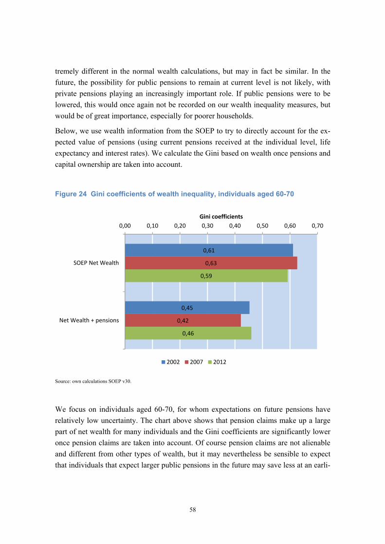
58
tremely different in the normal wealth calculations, but may in fact be similar. In the
future, the possibility for public pensions to remain at current level is not likely, with
private pensions playing an increasingly important role. If public pensions were to be
lowered, this would once again not be recorded on our wealth inequality measures, but
would be of great importance, especially for poorer households.
Below, we use wealth information from the SOEP to try to directly account for the ex-
pected value of pensions (using current pensions received at the individual level, life
expectancy and interest rates). We calculate the Gini based on wealth once pensions and
capital ownership are taken into account.
Figure 24 Gini coefficients of wealth inequality, individuals aged 60-70
Source: own calculations SOEP v30.
We focus on individuals aged 60-70, for whom expectations on future pensions have
relatively low uncertainty. The chart above shows that pension claims make up a large
part of net wealth for many individuals and the Gini coefficients are significantly lower
once pension claims are taken into account. Of course pension claims are not alienable
and different from other types of wealth, but it may nevertheless be sensible to expect
that individuals that expect larger public pensions in the future may save less at an earli-
0,61
0,45
0,63
0,42
0,59
0,46
0,00 0,10 0,20 0,30 0,40 0,50 0,60 0,70
SOEP Net Wealth
Net Wealth + pensions
Gini coefficients
2002 2007 2012

59
er stage in life, and therefore that for some low savings will not translate in low con-
sumption after retirement.
Finally, we look into the issue of different types of wealth. Using the data from the
SOEP at face value although we know that they may not be perfect, we look at the Gini
coefficients for overall net wealth, and then separately for real assets and financial as-
sets. We find real assets to be less unequally distributed compared to financial assets.
We also find, perhaps surprisingly, inequality in real assets to be highest among young
individuals, and lower among older individuals, probably because large home owner-
ship shares among older individuals.
Figure 25 Gini coefficients of real and financial assets
Source: own calculations from SOEP v30.
0,45 0,5 0,55 0,6 0,65 0,7 0,75
Net Wealth
Real Assets
Financial Assets
Gini Coefficients
Overall Age 16‐35 Age 36‐50 Age 51‐65 Age 66+

60
13. ECB policy and inequality
If households that are at different points of the net wealth distribution systematically
hold a different share of their wealth in certain types of assets, macroeconomic policy
changes, such as those affecting interest rates, will have distributional effects, because
different types of assets respond differently to interest rates. In a context in which banks
increasingly invest in already existing assets , such as fixed supply (most predominantly
real estate) most, if not all of the beneficial effects for lenders will disappear because it
will be passed on to prices. In addition, larger debtors are unlikely to come from the
bottom of the wealth distribution. Holzhausen and Sikova (2015) also use the HFCS
dataset to look at the effects of low interest rates (as those generated by the large Quan-
titative Easing intervention of the ECB) on overall incomes, asset values, as well as dis-
tributional consequences. For the EU as a whole, and in a more pronounced fashion for
Germany, they find interest losses to be much larger (as a share of income) for low in-
come households. In Germany, while interest losses they are close to one percent of
annual income for the lower quintile, they are around 0.4 percent of annual income for
the top quintile. Losses are much smaller in other EU countries including France, Spain
and Greece. Interest gains on loans are higher for higher income groups in absolute val-
ue, but the difference among income groups is not very large in Germany (Holzhausen
and Sikova 2015, page 29). When we net out interest gains and interest losses, effects
are very heterogeneous across countries.
In Germany, low interest rates seem to be about regressive redistribution, i.e. ‘from the
bottom to the top’, i.e. increased wealth inequality.17 Germany is indeed the only coun-
try where effects for the first two quintiles of the income distribution are negative, while
they are positive for the top two quintiles. Holzhausen and Sikova (2015) do not com-
ment on this, but our view is that is has a lot to do with differences in the types of assets
that different groups of individuals own, and in particular with the housing market.
German households that are at the lower end of the wage distribution are much less like-
ly to have a mortgage compared to Spanish and Dutch households (as our calculations
on home ownership show), and therefore do not stand to gain from lower interest rates.
Therefore, in the case of German households, the negative effect that goes through low-
er interest income on deposits dominates. The low interest rates policy of the European
Central Bank seems to have heterogeneous effects on inequality, depending on the level
at which we concentrate. Using the HFCS dataset, Bernoth, König, and Beckers (2016)
17 Our analysis looks at the effects of interest rates on the value of different assets. We believe that commenting on
the effects of low interest rates operating through potentially higher economic growth would be purely speculative.

61
also investigate the effects of the ECB monetary policy on the distribution of wealth.
Increases in asset prices tend to benefit richer households disproportionately. Indeed,
they show that households over the 75th percentiles are the only group that has stock
ownership large enough to be strongly affected by stock prices. Households with medi-
um and medium-high net wealth are much more strongly affected by housing prices.
Looking at the Euro area as a whole, it may have had overall positive income effects in
the Euro area (negative effects in Germany, however). There may have been also been
inequality-decreasing effects between countries, with richer countries such as Germany
losing and relatively poor countries such as Spain, Greece and Italy gaining. However,
the distributional effects within countries seem to have worked differently. In particular,
in countries such as Germany, poorer households have lost, while households above the
60th income percentile have gained. The message from this is also that the distributional
effects of macroeconomic policies are likely to be very different across countries, be-
cause the distribution of asset ownership (both quantity and type) across income groups
varies greatly across countries. Looking at Germany alone, one would conclude that
Quantitative East increases inequality. However, in other countries this is not the case.
In order to evaluate the effects of such policies, initial conditions of each economy is
crucial.

62
14. Discussion and policy implications
While inequality is a central topic both in the scientific and in the political discussion in
Germany, we believe that the debate is at times incomplete or even misleading. In this
report, we present a set of empirical facts concerning inequality in Germany in its dif-
ferent aspects, including wage, income and wealth inequality, the role of compositional
effects on the way we measure inequality. We believe that there are some trends in the
labour market and in the economy as a whole that may imply that our measures of ine-
quality is higher than it would otherwise be, but that either cannot be stopped, or are
even desirable for a society. These include for example population ageing, higher edu-
cational attainments and higher labour market participation of sections of individuals
that are less qualified. The evidence we present is a positive use, but we believe that it
suggests that many of the policies proposed to tackle inequality starting from a narrow
view of it are likely to be ineffective or damaging.
Much of the debate on inequality does not specifically address the relationship between
inequality and efficiency, and typically views classical redistributive policies as the
main (or only) channel through which inequality can be affected. As Keuschnigg (2015)
also points out, viewing the efficiency/equity as a tradeoff in all cases and for all con-
texts is naïve and may be misleading. There may be policy aimed at increasing alloca-
tive efficiency of an economy, which may at the same time decrease inequality, by in-
creasing opportunities to those that do not have them or regulating those who may have
positional rents. A natural example is education policy, as discussed in Keuschnigg
(2015). The introduction of tuition fees paired with generous student loans and grants
for bright students from low socio-economic backgrounds may increase efficiency and
decrease inequality at the same time. Education, training and competition are of crucial
importance. To the extent that they lay an important role for before-tax income inequali-
ty, there seems to be room for improvement in Germany. Upward social mobility is pos-
sible insofar as talented children from parents from a disadvantaged background are
given the information and opportunity to attain the highest levels of education. In a con-
text where technological change tends to favour workers with higher levels of educa-
tion, the strong correlation between educational attainments across generations is one of
the main sources of higher levels of inequality in before tax incomes. Failing to recog-
nize talent irrespective of parental background is also wasteful from a societal stand-
point, and is a clear example that, unlike policies aiming at static income distribution,
once we focus on before tax inequality one can move out the tradeoff between inequali-
ty and growth, rather than having to navigate it. The economic literature seems to have
63
reached a consensus that interventions in early education might have the highest returns
(see Nores and Barnett 2010 for a review of international evidence from this literature).
Most recently, Waldfogel (2015) discusses a number of US and European studies that
improvements in pre-school availability are indeed stronger for children coming from
disadvantaged background, implying that early interventions of this type have positive
outcomes in terms of equality of opportunities and efficiency. In Germany, additional
public funding for early education might be necessary. The funding for these programs
does not need to come from additional taxation. Rather, the funding could come from
cost savings coming from means-tested tuition fees for higher education, where tuition-
free systems are often found to be regressive.
Competition polices are also likely to play an important role in generating the before tax
income inequality. This is also a policy area where the same policy recommendations
that may decrease before tax income inequality might also promote overall economic
growth, and especially inclusive growth, where the gains from economic growth are not
concentrated in rent-seeking activities. To the extent that top incomes are the results of a
lack of competition, they are unlikely to be beneficial for upward mobility and ultimate-
ly for overall welfare. However, rather than confiscatory indiscriminate taxes for all
high incomes, it is important to focus on the mechanism behind income generation, try-
ing to fight rent-seeking activities and monopolistic practices where they exist, without
negatively affecting healthy wealth creation through productive activities. A recent
study by New Social Market Economy (INSM) has found that while Germany ranks
very well in composite measures of inequality, it ranks only 14th (among 28 OECD
members) on equality of opportunity, in particular in the areas of female labour force
participation and equality of opportunity in the education system. And this once again is
an example of how focusing on cross sectional inequality and tax redistribution alone is
not very helpful.
We believe that any serious analysis of inequality in Germany should not analyse
inequality based on net incomes in isolation. Agreeing on goals and then deciding on
policies that may help us to reach them requires a careful interpretation of the trends we
observe empirically. Looking at before tax income inequality is also important because
it suggests that if we are able to find policy instruments that will decrease before tax
income inequality over time, we will then be able to free up resources for other
activities that the welfare state may cyrry out, and lower the extent of taxation without
affecting the welfare of those in the lower part of the income distribution. Cingano
(2014) offers a useful review of the economic mechanisms through which higher
inequality might hurt economic growth. His considerations suggest that policies aiming
at lowering before tax inequality might boost investment by individuals in the lower

64
part of the income distribution, including human capital investments. However, and this
needs to be stressed, the effects of some of the policies discussed below are likely to
occur over long periods of time, wich is perhaps the reason why they are less appealing
to politicians. Nevertheless, they are of great importance for future competitivity and for
the sustainabiliy of the welfare state. Economist (2014) also discusses the relationship
between inequality and growth, and points out that it is likely that some ways of
redistributing income are more healthy than others, and may actually promote growth.
At the same time, it is likely that very highly redistributive countries have shorter and
weaker growth spells.
65
References
Adam, Hermann. 2014. “Die Politische Ökonomie Wachsender Ungleichverteilung Der Einkommen.” Wirtschaftsdienst 94 (2): 104–11.
Antonczyk, Dirk, Bernd Fitzenberger, and Katrin Sommerfeld. 2010. “Rising Wage Inequality, the Decline of Collective Bargaining, and the Gender Wage Gap.” Labour Economics 17 (5). Elsevier: 835–47.
Bartels, Charlotte, and Carsten Schröder. 2016. “Zur Entwicklung von Top-Einkommen in Deutschland Seit 2001.” DIW Wochenbericht 83 (1). DIW Berlin, German Institute for Economic Research: 3–9.
Bernoth, Kerstin, Philipp König, and Benjamin Beckers. 2016. “EZB-Anleihekäufe Können Vermögensverteilung Beeinflussen.” DIW Wochenbericht Nr. 7.
Bundesbank, Deutsche. 2013. “Household Wealth and Finances in Germany: Results of the Bundesbank Survey.” Deutsche Bundesbank Monthly Report N. 23.
Card, David, Jörg Heining, and Patrick Kline. 2013a. “Workplace Heterogeneity and the Rise of West German Wage Inequality.” The Quarterly Journal of Economics 128 (3). Oxford University Press: 967–1015.
———. 2013b. “Workplace Heterogeneity and the Rise of West German Wage Inequality.” Quarterly Journal of Economics 128: 967–1015.
Cingano, Federico. 2014. “Trends in Income Inequality and Its Impact on Economic Growth.” OECD Social, Employment and Migration Working Papers, No. 163.
Dustmann, Christian, Bernd Fitzenberger, Uta Schönberg, and Alexandra Spitz-Oener. 2014. “From Sick Man of Europe to Economic Superstar: Germany’s Resurgent Economy.” Journal of Economic Perspectives 28: 167–88.
Dustmann, Christian, Johannes Ludsteck, and Uta Schönberg. 2009. “Revisiting the German Wage Structure.” The Quarterly Journal of Economics 124 (2). MIT Press: 843–81.
Economist. 2013. “Of Scissors and Biting.” The Economist May 9. http://www.economist.com/news/europe/21573115-inequality-germany-has-been-falling-it-still-firing-political-passions-scissors-and.
———. 2014. “Inequality v Growth.” The Economist March 1. http://www.economist.com/news/finance-and-economics/21597931-up-point-redistributing-income-fight-inequality-can-lift-growth-inequality.
Fessler, Pirmin, Peter Lindner, and Esther Segalla. 2014. “Net Wealth across the Euro Area - Why Household Structure Matters and How to Control for It.” ECB Working Paper 1663. European Central Bank..
Firpo, Sergio, Nicole M. Fortin, and Thomas Lemieux. 2009. “Unconditional Quantile Regressions.” Econometrica 77 (3). Econometric Society: 953–73.
Fitzenberger, Bernd. 2012. “Expertise Zur Entwicklung Der Lohnungleichheit in Deutschland.” German Council of Economic Experts Working Paper 04/2012.

66
German Council of Economic Experts / Sachverständigenrat zur Begutachtung der gesamtwirtschaftlichen Entwicklung.
Fuchs-Schuendeln, Nicola, Dirk Krueger, and Mathias Sommer. 2010. “Inequality Trends for Germany in the Last Two Decades: A Tale of Two Countries.” Review of Economic Dynamics 13 (1). Elsevier for the Society for Economic Dynamics:
Fuest, Clemens. 2016. “Zehn Thesen Zur Ungleichheitsdebatte.” Frankfurter Allgemeine Zeitung February 1 (2016).
Goebel, Jan, Markus M. Grabka, and Carsten Schröder. 2015. “Income Inequality Remains High in Germany: Young Singles and Career Entrants Increasingly At Risk of Poverty.” DIW Economic Bulletin 5 (25). DIW Berlin, German Institute for Economic Research: 325–39.
Grabka, Markus. 2015. “Income and Wealth Inequality after the Financial Crisis: The Case of Germany.” Empirica 42 (2). Springer: 371–90.
Grabka, Markus M., Jan Goebel, and Jürgen Schupp. 2012. “Has Income Inequality Spiked in Germany?” DIW Economic Bulletin 2 (12). DIW Berlin, German Institute for Economic Research: 3–14.
Grabka, Markus M., and Christian Westermeier. 2014. “Persistently High Wealth Inequality in Germany.” DIW Economic Bulletin 4 (6). DIW Berlin, German Institute for Economic Research: 3–15.
Heineck, Guido, and Regina T. Riphahn. 2009. “Intergenerational Transmission of Educational Attainment in Germany - The Last Five Decades.” Journal of Economics and Statistics (Jahrbuecher Fuer Nationaloekonomie Und Statistik) 229 (1). Justus-Liebig University Giessen, Department of Statistics and Economics: 36–60.
Holzhausen, Arne, and Sabina Sikova. 2015. “Low Interest Rates, Incomes and Assets: The Winners and the Losers.” Allianz Group Economic Research Working Paper N. 190.
Keuschnigg, Christian. 2015. “Ungleichheit, Das Richtige Maß.” Format 36. http://www.format.at/wirtschaft/oesterreich/ungleichheit-mass-5842044.
Klemm, Marcus, and Benjamin Weigert. 2014. “Does Composition Matter? Wage Inequality and the Demographic and Educational Structure of the Labor Force in Gemany.” Working Papers. German Council of Economic Experts / Sachverständigenrat zur Begutachtung der gesamtwirtschaftlichen Entwicklung.
Kuhn, Andreas. 2013. “Inequality Perceptions, Distributional Norms, and Redistributive Preferences in East and West Germany.” German Economic Review 14 (4). Verein für Socialpolitik: 483–99.
Möller, Joachim. 2016. “Lohnungleichheit - Gibt Es Eine Trendwende?” IAB Discussion Paper 9/2016.
Niehues, Judith. 2014. “Subjective Perceptions of Inequality and Redistributive Preferences: An International Comparison.” Cologne Institute for Economic Research Working Paper.

67
Nores, Milagros, and W. Steven Barnett. 2010. “Benefits of Early Childhood Interventions across the World: (Under) Investing in the Very Young.” Economics of Education Review 29 (2): 271–82.
Peichl, Andreas, Nico Pestel, and Hilmar Schneider. 2012. “Does Size Matter? The Impact Of Changes In Household Structure On Income Distribution In Germany.” Review of Income and Wealth 58 (1). International Association for Research in Income and Wealth: 118–41.
Schmid, Kai Daniel, and Ulrike Stein. 2013. “Explaining Rising Income Inequality in Germany, 1991-2010.” SOEPpapers on Multidisciplinary Panel Data Research. DIW Berlin, The German Socio-Economic Panel (SOEP).
Sinn, Hans-Werner. 2008. “Der Bedarfsgewichtete Käse Und Die Neue Armut.” Ifo Schnelldienst 61 (10). Ifo Institute for Economic Research at the University of Munich: 14–16.
Statistisches Bundesamt. 2015. Bildungsfinanzbericht 2015.
Stiglitz, Joseph E. 2015. “New Theoretical Perspectives on the Distribution of Income and Wealth among Individuals: Part IV: Land and Credit.” NBER Working Paper No. 21192. National Bureau of Economic Research, Inc.
Waldfogel, Jane. 2015. “The Role of Preschool in Reducing Inequality.” IZA World of Labor. Institute for the Study of Labor (IZA).
Ifo Working Papers
No. 216 Baumgarten, D., G. Felbermayr and S. Lehwald, Dissecting between-plant and within-
plant wage dispersion – Evidence from Germany, April 2016.
No. 215 Felbermayr, G., Economic Analysis of TTIP, April 2016.
No. 214 Karmann, A., F. Rösel und M. Schneider, Produktivitätsmotor Gesundheitswirtschaft:
Finanziert sich der medizinisch-technische Fortschritt selbst?, April 2016.
No. 213 Felbermayr, G., J. Gröschl and T. Steinwachs, The Trade Effects of Border Controls:
Evidence from the European Schengen Agreement, April 2016.
No. 212 Butz, A. und K. Wohlrabe, Die Ökonomen-Rankings 2015 von Handelsblatt, FAZ und
RePEc: Methodik, Ergebnisse, Kritik und Vergleich, März 2016.
No. 211 Qian, X. and A. Steiner, International Reserves, External Debt Maturity, and the Re-
inforcement Effect for Financial Stability, March 2016.
No. 210 Hristov, N., The Ifo DSGE Model for the German Economy, February 2016.
No. 209 Weber, M., The short-run and long-run effects of decentralizing public employment
services, January 2016.
No. 208 Felfe, C. and J. Saurer, Granting Birthright Citizenship – A Door Opener for Immigrant
Children’s Educational Participation and Success?, December 2015.
No. 207 Angerer, S., P. Lergetporer, D. Glätzle-Rützler and M. Sutter, How to measure time
preferences in children – A comparison of two methods, October 2015.
No. 206 Kluge, J., Sectoral Diversification as Insurance against Economic Instability, September
2015.
No. 205 Kluge, J. and M. Weber, Decomposing the German East-West wage gap, September 2015.
No. 204 Marz, W. and J. Pfeiffer, Carbon Taxes, Oil Monopoly and Petrodollar Recycling,
September 2015.

No. 203 Berg, T.O., Forecast Accuracy of a BVAR under Alternative Specifications of the Zero
Lower Bound, August 2015.
No. 202 Henderson, M.B., P. Lergetporer, P.E. Peterson, K. Werner, M.R. West and L. Woess-
mann, Is Seeing Believing? How Americans and Germans Think about their Schools,
August 2015.
No. 201 Reischmann, M., Creative Accounting and Electoral Motives: Evidence from OECD
Countries, July 2015.
No. 200 Angerer, S., D. Glätzle-Rützler, P. Lergetporer and M. Sutter, Cooperation and dis-
crimination within and across language borders: Evidence from children in a bilingual
city, May 2015.
No. 199 Schulz, B., Wage Rigidity and Labor Market Dynamics with Sorting, May 2015.
No. 198 Jochimsen, B. and R. Lehmann, On the political economy of national tax revenue fore-
casts – Evidence from OECD countries, March 2015.
No. 197 Marz, W. and J. Pfeiffer, Resource Market Power and Levels of Knowledge in General
Equilibrium, March 2015.
No. 196 Lehmann, R., Survey-based indicators vs. hard data: What improves export forecasts in
Europe?, March 2015.
No. 195 Fabritz, N., ICT as an Enabler of Innovation: Evidence from German Microdata, January 2015.
No. 194 Kauder, B. and N. Potrafke, Just hire your spouse! Evidence from a political scandal in
Bavaria, December 2014.
No. 193 Seiler, C., Mode Preferences in Business Surveys: Evidence from Germany, Novem-
ber 2014.
No. 192 Kleemann, M. and M. Wiegand, Are Real Effects of Credit Supply Overestimated? Bias
from Firms' Current Situation and Future Expectations, November 2014.
No. 191 Kauder, B, Spatial Administrative Structure and Intra-Metropolitan Tax Competition,
October 2014.
Top Related