


Languages
Pages
Legal


Incremental Potential Contact: Intersection- and Inversion-free,Large-Deformation Dynamics
MINCHEN LI, University of Pennsylvania & Adobe Research
ZACHARY FERGUSON and TESEO SCHNEIDER, New York University
TIMOTHY LANGLOIS, Adobe ResearchDENIS ZORIN and DANIELE PANOZZO, New York University
CHENFANFU JIANG, University of Pennsylvania
DANNY M. KAUFMAN, Adobe Research
Fig. 1. Squeeze out: Incremental Potential Contact (IPC) enables high-rate time stepping, here with h = 0.01s, of extreme nonlinear elastodynamics with
contact that is intersection- and inversion-free at all time steps, irrespective of the degree of compression and contact. Here a plate compresses and then
forces a collection of complex soft elastic FE models (181K tetrahedra in total, with a neo-Hookean material) through a thin, codimensional obstacle tube. The
models are then compressed entirely together forming a tight mush to fit through the gap and then once through they cleanly separate into a stable pile.
Contacts weave through every aspect of our physical world, from daily
household chores to acts of nature. Modeling and predictive computation of
these phenomena for solid mechanics is important to every discipline con-
cerned with the motion of mechanical systems, including engineering and
animation. Nevertheless, efficiently time-stepping accurate and consistent
simulations of real-world contacting elastica remains an outstanding com-
putational challenge. To model the complex interaction of deforming solids
in contact we propose Incremental Potential Contact (IPC) ś a new model
and algorithm for variationally solving implicitly time-stepped nonlinear
Authors’ addresses: Minchen Li, University of Pennsylvania & Adobe Research,[email protected]; Zachary Ferguson; Teseo Schneider, New York University;Timothy Langlois, Adobe Research; Denis Zorin; Daniele Panozzo, New York Univer-sity; Chenfanfu Jiang, University of Pennsylvania; Danny M. Kaufman, Adobe Research,[email protected].
Permission to make digital or hard copies of all or part of this work for personal orclassroom use is granted without fee provided that copies are not made or distributedfor profit or commercial advantage and that copies bear this notice and the full citationon the first page. Copyrights for components of this work owned by others than ACMmust be honored. Abstracting with credit is permitted. To copy otherwise, or republish,to post on servers or to redistribute to lists, requires prior specific permission and/or afee. Request permissions from [email protected].
© 2020 Association for Computing Machinery.0730-0301/2020/7-ART49 $15.00https://doi.org/10.1145/3386569.3392425
elastodynamics. IPC maintains an intersection- and inversion-free trajectory
regardless of material parameters, time step sizes, impact velocities, severity
of deformation, or boundary conditions enforced.
Constructed with a custom nonlinear solver, IPC enables efficient res-
olution of time-stepping problems with separate, user-exposed accuracy
tolerances that allow independent specification of the physical accuracy of
the dynamics and the geometric accuracy of surface-to-surface conformation.
This enables users to decouple, as needed per application, desired accuracies
for a simulation’s dynamics and geometry.
The resulting time stepper solves contact problems that are intersection-
free (and thus robust), inversion-free, efficient (at speeds comparable to or
faster than available methods that lack both convergence and feasibility),
and accurate (solved to user-specified accuracies). To our knowledge this
is the first implicit time-stepping method, across both the engineering and
graphics literature that can consistently enforce these guarantees as we vary
simulation parameters.
In an extensive comparison of available simulation methods, research
libraries and commercial codes we confirm that available engineering and
computer graphics methods, while each succeeding admirably in custom-
tuned regimes, often fail with instabilities, egregious constraint violations
and/or inaccurate and implausible solutions, as we vary input materials,
contact numbers and time step. We also exercise IPC across a wide range
ACM Trans. Graph., Vol. 39, No. 4, Article 49. Publication date: July 2020.

49:2 • Minchen Li, Zachary Ferguson, Teseo Schneider, Timothy Langlois, Denis Zorin, Daniele Panozzo, Chenfanfu Jiang, and Danny M. Kaufman
of existing and new benchmark tests and demonstrate its accurate solution
over a broad sweep of reasonable time-step sizes and beyond (up to h = 2s)
across challenging large-deformation, large-contact stress-test scenarios
with meshes composed of up to 2.3M tetrahedra and processing up to 498K
contacts per time step. For applications requiring high-accuracy we demon-
strate tight convergence on all measures. While, for applications requiring
lower accuracies, e.g. animation, we confirm IPC can ensure feasibility and
plausibility even when specified tolerances are lowered for efficiency.
CCS Concepts: • Computing methodologies→ Physical simula-
tion.
Additional Key Words and Phrases:Contact Mechanics, Elastodynamics,
Friction, Constrained Optimization
ACM Reference Format:
Minchen Li, Zachary Ferguson, Teseo Schneider, Timothy Langlois, Denis
Zorin, Daniele Panozzo, Chenfanfu Jiang, and Danny M. Kaufman. 2020. In-
cremental Potential Contact: Intersection- and Inversion-free, Large-Deformation
Dynamics. ACM Trans. Graph. 39, 4, Article 49 (July 2020), 20 pages. https:
//doi.org/10.1145/3386569.3392425
1 INTRODUCTION
Contact is ubiquitous and often unavoidable and yet modeling con-
tacting systems continues to stretch the limits of available computa-
tional tools. In part this is due to the unique hurdles posed by contact
problems. There are several intricately intertwined physical and
geometric factors that make contact computations hard, especially
in the presence of friction and nonlinear elasticity.
Real-world contact and friction forces are effectively discontin-
uous, immediately making the time-stepping problems very stiff,
especially if the contact constraints are enforced exactly. On the
other hand, even small violations of exact contact constraints (which
are nonconvex) can lead to impossible to untangle geometric config-
urations, with a direct impact on physical accuracy and stability. In
addition, stiff contact forces often lead to extreme deformations, re-
sulting in element inversions for mesh-based discretization. Friction
modeling then introduces further challenges with asymmetric force
coupling and rapid switching between sliding and sticking modes.
In this work, our goal is to achieve very high robustness (by
which we mean the absence of catastrophic failures or stagnation)
for contact modeling even for the most challenging elastodynamic
contact problems with friction. Robustness should be obtained in-
dependent of user-controllable accuracy in time-stepping, spatial
discretization and contact resolution, while maintaining efficiency
required to solve large-scale problems. At the same time we wish to
also ensure that all accuracies ś across the board ś are efficiently
attainable (of course with additional cost) when required.
With these goals in mind, we reexamine the contact problem
formulation, discretization and numerical methods from scratch,
building on numerous ideas and observations from prior work.
Our Incremental Potential Contact (IPC) solver is constructed
for mesh-based discretizations of nonlinear volumetric elastody-
namic problems supporting large nonlinear deformations, implicit
time-steppingwith contact, friction and boundaries of arbitrary codi-
mension (points, curves, surfaces, and volumes). A key principle we
follow is that while the physics and shape can be approximated arbi-
trarily coarsely, the geometric constraints (absence of intersections
of the approximate geometry and inversions of elements) are main-
tained exactly at all times. We achieve this for essentially arbitrary
target time steps and spatial discretization resolution.
The key element of our approach is the formulation of the con-
tact problem and the customized numerical method to solve it. As
a starting point, we use an exact contact constraint formulation,
described in terms of an unsigned distance function, and rate-based
maximal dissipation for friction.
For every time step, we solve the discrete nonlinear contact prob-
lem with a given tolerance using a smoothed barrier method, ensur-
ing that the solution remains intersection-free at all intermediate
steps. We use a comparably smoothed, arbitrarily close, approxi-
mation to static friction, also eliminating the need for an explicit
Coulomb constraint, and cast friction forces at every time step in a
dissipative potential form, using an alternating lagged formulation.
All forces can then be solved by unconstrained minimization.
Our barrier formulation for contact has several important prop-
erties: 1) it is an almost everywhere C2 function of the unsigned
distances between mesh elements,C1 continuous for a measure-zero
set of configurations; 2) its support is restricted to a small part of the
configuration space close to configurations with contact. The former
property makes it possible to use rapidly converging Newton-type
unconstrained optimization methods to solve the barrier approxima-
tion of the problem, the latter ensures that additional contact forces
are applied highly locally and that only a small set of terms of the
barrier function need to be computed explicitly during optimization.
Jointly they enable stable, conforming contact between geometries.
To guarantee a collision-free state at every time step, feasibility
is maintained throughout all nonlinear solver iterations: the line
search in our customized Newton-based solver is augmented with
efficient, filtered continuous collision detection (CCD) accelerated
by a conservative CFL-type contact bound on line search step sizes.
Friction forces are resolved directly in the same solver via our lagged
potential with geometric accuracy improved by alternating updates.
1.1 Contributions
In summary, IPC solves nonlinear elastodynamic trajectories that
are intersection- and inversion-free, efficient and accurate (solved
to user-specified accuracies) while resolving collisions with both
nonsmooth and codimensional obstacles. To our knowledge, this is
the first implicit time-stepping method, across both the engineering
and graphics literature, with these properties.
We demonstrate the efficacy of IPC with stress tests containing
large deformations, many contact primitive pairs, large friction,
tight collisions as well as sharp and codimensional obstacles. Our
technical contributions include
• A contact model based on the unsigned distance function;
• An almost everywhere C2, C1-continuous barrier formulation,
approximating the contact problem with arbitrary accuracy, with
barrier support localized in the configuration space, enabling
efficient time-stepping;
• Contact-aware line search that continuously guarantees penetration-
free descent stepswith CCD evaluations accelerated by a conservative-
bound contact-specific CFL-inspired filter;
ACM Trans. Graph., Vol. 39, No. 4, Article 49. Publication date: July 2020.

Incremental Potential Contact: Intersection- and Inversion-free, Large-Deformation Dynamics • 49:3
• A new variational friction model with smoothed static friction,
formulated as a lagged dissipative potential, robustly resolving
challenging frictional contact behaviors; and
• A new benchmark of simulation test sets with careful evalua-
tion of constraint and time stepping formulations along with an
extensive evaluation of existing contact solvers.
2 CONTACT MODEL
We focus on solving numerical time-integration for nonlinear vol-
umetric elastodynamic models with contact. These models can in-
teract with fixed and moving obstacles which can be of arbitrary
dimension (surfaces, curves and points). The simulation domain is
discretized with finite elements. Given n nodal positions, x , finite-
element mass matrix, M , and a hyper-elastic deformation energy,
Ψ(x), the contact problem extremizes the extended-value action
S(x) =
∫ T
0
( 1
2ÛxTM Ûx − Ψ(x) + xT (fe + fd )
)
dt .
on an admissible set of trajectories A, which we discuss below. Here
fe are external forces and fd are dissipative frictional forces. We
assume, for simplicity, that all object geometry is discretized with
n-dimensional piecewise-linear elements, n = 1, 2, 3.
Admissible trajectories. We construct a new definition of admissi-
bility based on unsigned distance functions that has a number of
advantages. Most importantly, in the context of our work, it nat-
urally allows us to formulate exact contact constraints in terms
of constraints on collisions between pairs of primitives (triangles,
vertices and edges), and can be defined in exactly the same way for
objects of any dimensions (points, curves, surfaces and volumes).
Specificallywe define trajectoriesx(t), withx ∈ R3n as intersection-
free, if for all moments t , x(t) ensures that the distance d(p,q) be-
tween any distinct points p and q on the boundaries of objects is
positive. In the space of trajectories, the set of intersection-free
trajectories forms an open set AI , as it is defined by strict inequal-
ities. Optimization problems may not have solutions in this set;
for this reason, we add the limit trajectories to it, which involve
contact. Specifically, we define the set of admissible trajectories A
as the closure of AI . In other words, a trajectory is admissible, if
it is intersection-free, or there is an intersection-free trajectory
arbitrarily close.
Note that this closure is not equivalent to replacing the constraint
d(p,q) > 0withd(p,q) ≥ 0; the latter is always satisfied for unsigned
distances, so that all trajectories would be admissible. This is not
the case for our definition. Consider for example, a point moving
towards a plane. If its trajectory touches the plane and then turns
back, an arbitrarily small perturbation makes it intersection-free,
and the trajectory is in A. However, if the trajectory crosses the
plane small perturbations do not make it intersection-free. This
highlights the need for our treatment even in the volumetric setting
as the boundaries of our mesh upon which we impose constraint are
exactly surfaces whose potential collisions include the point-face
case above.
We can describe AI directly in terms of constraints on unsigned
distances d between surface primitives (vertices, edges, and faces in
the simulation surfacemesh and domain boundaries).We denote this
set of mesh primitivesT . Equivalently to themore general definition
above, a piecewise-linear trajectory x(t) starting in an intersection-
free state x0 is admissible, if for all times t , the configuration x(t)
satisfies positive distance constraints di j (x(t)) > 0 for all {i, j} ∈ B,
where B ⊂ T × T is the set of all non-adjacent and non-incident
surface mesh primitive pairs.
We then observe that the distance between any pair of primi-
tives is bounded from below by the distance for triangle-vertex and
edge-edge pairs, if there are no intersections. For this reason, it is
sufficient to enforce constraints dk (x(t)) > 0 continuously in time,
for all k ∈ C ⊂ B where C contains all non-incident point-triangle
and all non-adjacent edge-edge pairs in the surface mesh.
Time discretization. Discretizing in time, we can directly construct
discrete energies whose stationary points give an unconstrained
time step method’s update [Ortiz and Stainier 1999]. Concretely,
given nodal positions xt and velocities vt , at time step t , we formu-
late the time step update for new positions xt+1 as the minimization
of an Incremental Potential (IP) [Kane et al. 2000], E(x, xt ,vt ), over
valid x ∈ R3n . For example the IP for implicit Euler is then simply
E(x, xt ,vt ) = 12 (x − x)
TM(x − x) − h2xT fd + h2Ψ(x), (1)
where h is the time step size and x = xt + hvt + h2M−1 fe . IPs
for implicit Newmark (see Section 7) and many other integrators
follow similarly by simply treating their update rule as stationarity
conditions of a potential with respect to variations of xt+1.
Addition of contact constraints restricts minimization of the IP
to admissible trajectories [Kane et al. 1999; Kaufman and Pai 2012]
and so yields for our model the following time step problem:
xt+1 = argminx
E(x, xt ,vt ), xτ ∈ A, (2)
where xτ , τ ∈ [t, t + 1], is the linear trajectory between xt and xt+1.
Our goal is to define a numerical method for approximating the
solution of this problem in (2). Solving it is challenging due to the
complex nonlinearity of the admissibility constraint, especially in
the context of large deformations.
In turn, when frictional forces in (2) include frictional contact,
solving the time step problem becomes all the more challenging as
fd is now governed by the Maximal Dissipation Principle [Moreau
1973] and so must satisfy further challenging, asymmetric and
strongly nonlinear consistency conditions [Simó and Hughes 1998].
We present a friction formulation in Section 5 that is naturally inte-
grated into this formulation via a lagged dissipative potential.
We further define a set of piecewise-linear surfaces as ϵ-separated,
if the distance between two boundary points of the set is at least
ϵ , unless these are on the same element of the boundary. An ϵ-
separated trajectory is then a trajectory for which surfaces stay
ϵ-separated. We denote the set of such trajectories Aϵ .
To handle contact constraints, in our algorithm, we use the fol-
lowing overall approach: (a) the IP function E is unmodified on Aϵ
ś the set of trajectories for which any ϵ-separated trajectory extrem-
izes the action are preserved; (b) we introduce a barrier term that
vanishes for trajectories inAϵ and diverges as the distance between
any two boundary points vanishes, converting the problem to an
unconstrained optimization problem. This barrier, together with
ACM Trans. Graph., Vol. 39, No. 4, Article 49. Publication date: July 2020.

49:4 • Minchen Li, Zachary Ferguson, Teseo Schneider, Timothy Langlois, Denis Zorin, Daniele Panozzo, Chenfanfu Jiang, and Danny M. Kaufman
continuous collision detection within minimization steps, ensure
that trajectories remain in AI .
This algorithm then guarantees that the trajectories are modi-
fied, compared to the exact solution, in an arbitrarily small, user-
controlled (by ϵ) region near object boundaries and, at the same
time, always remain admissible.
2.1 Trajectory accuracies
A discrete contacting trajectory is accurate if it satisfies 1) admis-
sibility, 2) discrete momentum balance, 3) positivity, 4) injectivity
and 5) complementarity.
In the discrete setting, momentum balance requires that the gradi-
ent of the incremental potential, ∇xE(x), balance against the time-
integrated contact forces. Its accuracy, is then exactly measured by
the residual error in the optimization of the constrained incremental
potential. We simply and directly control accuracy of momentum
balance by setting stopping tolerance in our nonlinear optimization;
see Section 4.5.
In turn positivity means that contact forces’ signed magnitudes,
λk , per contact pair k ∈ C, are always non-negative and so push
surfaces but do not pull. Our method guarantees exact positivity.
Combined with admissibility, injectivity requires positive volumes
for all tetrahedra in the simulation mesh. This invariant is enforced
when a non-inverting energy density function, e.g. neo-Hookean, is
modeled 1.
Finally, the classic definition of complementarity in contact me-
chanics [Kikuchi and Oden 1988] is the requirement that contact
forces enforcing admissibility can only be exerted between surfaces
if they are touching with no distance between them. We do not
allow dk (x) = 0, and so define a comparable measure of discrete
ϵ-complementarity requiring
λk max(0,dk (x) − ϵ) = 0, ∀k ∈ C (3)
to measure how well contact accuracy is achieved. Discrete comple-
mentarity is then satisfied whenever distances between all contact
pairs, defined as surface pairs with nonzero contact forces, are less
than the ϵ and converge to complementarity as we reduce ϵ .
3 RELATED WORK
Computational contact modeling is a fundamental and long studied
task in mechanics well covered from diverse perspectives in engi-
neering, robotics and computer graphics [Brogliato 1999; Kikuchi
and Oden 1988; Stewart 2001; Wriggers 1995]. At its core the con-
tact problem combines enforcement of significant and challenging
geometric non-intersection constraints with the resolution of a de-
formable solid’s momentum balance. The latter task is well-explored,
often independent of contact [Belytschko et al. 2000; Stuart and
Humphries 1996]. We focus below on related works in defining con-
tact constraints, implicitly time stepping with contact and friction,
and barriers.
1When an invertible deformation model, e.g. fixed corotational, is modeled, injectivityneed not be preserved in computation. We primarily focus on non-inverting neo-Hookean but will also demonstrate the weaker invertible case with fixed corotational.
3.1 Constraints and constraint proxies
Contact simulation requires a computable model of admissibility
and so a choice of contact constraint representation. For volumetric
models, admissibility generally begins with description of a signed
distance function. This allows a clean formulation of the continuous
model. However, when it comes to computing non-intersection
on deformable meshes, choices for representing non-intersection
must be made and a diversity of constraint representations exist.
Contact constraints for deformable meshes, in both engineering
[Belytschko et al. 2000; Wriggers 1995] and graphics [Bridson et al.
2002; Daviet et al. 2011; Harmon et al. 2009, 2008; Otaduy et al. 2009;
Verschoor and Jalba 2019] are most commonly defined pairwise
between matched surface primitives.
Existing methods most often define a local, signed distance eval-
uation using a diverse array of nonlinear proxy functions as well as
their linearizations. These include linear gap functions, linearized
constraints built from geometric normals, as well as a number of
oriented volume constraints [Kane et al. 1999; Sifakis et al. 2008].
These nonlinear proxies, such as the tetrahedral volumes formed be-
tween surface point-face and edge-edge pairs, are only locally valid.
They can introduce artificial ghost contact forces when sheared,
false positives when rotated (e.g. for edge-edge tetrahedra), discon-
tinuities when traversing surface element boundaries, and, in many
methods, must still be further linearized and so introduce additional
levels of approximation in order to solve a constrained time step.
Alternately gap functions and other related methods approxi-
mate signed distance functions for pairs of primitives by locally
projecting a linearized distance measure between pairwise surface
primitives onto a fixed geometric normal [Otaduy et al. 2009; Wrig-
gers 1995]. As discussed in Erleben [Erleben 2018] these łcontact
point and normalž based constraint functions can be inconsistent
over successive iterations and so are highly sensitive to surface and
meshing variations with well known failure modes if care is not
taken. Indeed, as we investigate in Section 8.3, even with iterative
updates of these linear constraints inside SQP-type methods, time
stepping with gap functions and related representations produces
highly varied results whose success or failure is largely dependent
on the scene simulated. In turn all of these challenges are only fur-
ther exacerbated when simulations encounter the sharp, nonsmooth
and even codimensional collisions imposed by meshed obstacles
[Kane et al. 1999]; see e.g. Figure 2.
Fig. 2. Nonsmooth, codimensional
collisions. Left: thin volumetric mat
falls on codimensional (triangle) ob-
stacles. Right: a soft ball falls on a ma-
trix of point obstacles, front and bot-
tom views.
Recent fictitious domain
methods [Jiang et al. 2017;
Misztal and Bñrentzen 2012;
Müller et al. 2015; Pagano
and Alart 2008; Zhang et al.
2005] offer a promising al-
ternative. In these meth-
ods, motivated by global
injectivity conditions [Ball
1981] negative space is sep-
arately discretized by a
compatible discretization
sometimes called an air-
mesh [Müller et al. 2015].
ACM Trans. Graph., Vol. 39, No. 4, Article 49. Publication date: July 2020.

Incremental Potential Contact: Intersection- and Inversion-free, Large-Deformation Dynamics • 49:5
Maintaining a non-negative volume on elements of this mesh then
guarantees non-inversion. However, as with locally defined proxy
volumes, the globally defined mesh introduces increasingly severe
errors, e.g., shearing and locking forces, as it distorts with the mate-
rial mesh. In 2D this can be alleviated by local [Müller et al. 2015]
or global [Jiang et al. 2017] remeshing, however this is highly ineffi-
cient in 3D, does not provide a continuous constraint representation
for optimization, nor, even with remeshing, can it resolve sliding and
resting contact where air elements must necessarily be degenerate
[Li et al. 2018].
Alternately, discrete signed distance fields (SDF) representations
can be constructed via a number of approximation strategies over
spatial meshes [Jones et al. 2006]. However, while state of the art
adaptive SDF methods now gain high-resolution accuracy for sam-
pling against a fixed meshes [Koschier et al. 2017], they can not
yet be practically updated at rates suitable for deformable time
steps, much less at rates suitable for querying deformations at ev-
ery iterate within a single implicit time step solve [Koschier et al.
2017]. At the same time, discontinuities across element boundaries,
while improved in recent works, still preclude smooth optimization
methods.
We observe that while approximating signed distance pairwise
between surface mesh elements is problematic, unsigned distance is
well defined. We then design a new contact model for exact admis-
sibility constraints in terms of unsigned distances between mesh-
element pairs. This model of constraint is constructed sufficiently
smooth to enable efficient, super-linear Newton-type optimization,
maintains exact constraint satisfaction guarantees throughout all
steps (time steps and iterations) and requires evaluation of just
mesh-surface primitive pairs.
3.2 Implicit Time Step Algorithms for Contact
With choice of contact constraint proxy, д(x) ≥ 0, the solve for the
implicit time-step update is then the minimization of the contact-
constrained IP [Doyen et al. 2011; Kane et al. 1999; Kaufman and
Pai 2012],
minx
E(x, xt ,vt ) s.t. д(x) ≥ 0. (4)
The variational problem (4), or its approximation is then minimized
to compute the configuration at each time step.
This is typically done with off-the-shelf [Nocedal and Wright
2006] or customized constrained optimization techniques. In en-
gineering, commonly used methods include sequential quadratic
programming (SQP) [Kane et al. 1999], augmented Lagrangian and
occasionally interior point methods [Belytschko et al. 2000]. All
such methods iteratively linearize constraint functions and elasticity.
However, both nonlinear constraint functions and their lineariza-
tions are generally valid only in local regions of evaluation and so
can lead to intersections due to errors at larger time steps, faster
speeds and/or larger deformations. For example Kane et al.’s [1999]
volumes are only valid under a strong assumption of the relative
position of contact primitive pairs.
In turn linearization of the full constraint set can also introduce
additional error, result in infeasible sub-problems, locking and/or
constraint drift [Erleben 2018]. This often requires complex and chal-
lenging (re-)evaluations of constraints in inter-penetrating states.
Even when such obstructions are not present, iterated constraint
linearization generally can not guarantee interpenetration-free state
except upon convergence and so often must resort to small time
steps and non-physical fail-safes in order to limit damage caused by
missed constraint enforcement.
Although SQP- [Kane et al. 1999] and LCP/QP-based contact
solvers [Kaufman et al. 2008] support and generally employ a va-
riety of constraint-set culling and active-set update strategies, e.g.,
incrementally adding newly detected collisions at each iteration
[Otaduy et al. 2009; Verschoor and Jalba 2019], they also can be-
come infeasible and generate constraint drift when linearizing and
filtering constraints.
Irrespective of how the contact-IP is solved and constraints are
enforced, we then remain faced with combinatorial explosion in the
number of contact constraints to handle. Determining the active
set, i.e., finding which constraints are necessary for admissibility
and so can not be ignored, remains an outstanding computational
challenges. At the same time, to take large time steps or handle
large deformation, we must resolve strongly nonlinear deformation
energies in balance with contact forces. This requires line search.
However, for constrained optimization methods, e.g., SQP, efficient
line search in the presence of large numbers of active constraints
remains an open problem [Bertsekas 2016; Nocedal and Wright
2006]. For this reason, existing methods in graphics currently avoid
line search altogether and are, as a consequence, mostly restricted to
quadratic energymodels per time step [Otaduy et al. 2009; Verschoor
and Jalba 2019] and, often, small time step sizes for even moderate
material stiffness [Verschoor and Jalba 2019].
3.3 Friction
The addition of accurate friction with stiction only increases the
computational challenge for time stepping deformation [Wriggers
1995]. Friction forces are tightly coupled to the computation of both
deformation and the contact forces that prevent intersection. These
side conditions are generally formulated by their own governing
variational Maximal Dissipation Principle (MDP) [Goyal et al. 1991;
Moreau 1973] and thus introduce additional nonlinear, nonsmooth
and asymmetric relationships to dynamics. In transitions between
sticking and sliding modes large, nonsmooth jumps in both mag-
nitude and direction are made possible by frictional contact model.
Asymmetry, in turn, is a direct consequence ofMDP: frictional forces
are not uniquely defined by the velocities they oppose, and are also
determined by additional consistency conditions and constraints,
e.g., Coulomb’s law. One critical consequence is that there is no
well-defined potential that we can add to an IP to directly produce
contact friction via minimization.
To address these challenges, frictional contact is often solved by
seeking a joint solution to the optimality conditions ofMDP together
with the discretized equations of motion (the latter are equivalent to
optimality conditions for E). This requires, however, simultaneously
solving for primal velocity unknowns together with a large addi-
tional number of dual contact and friction force unknowns. These
latter variables then scale in the number of active contacts and their
number grows large for even moderately sized simulation meshes.
ACM Trans. Graph., Vol. 39, No. 4, Article 49. Publication date: July 2020.

49:6 • Minchen Li, Zachary Ferguson, Teseo Schneider, Timothy Langlois, Denis Zorin, Daniele Panozzo, Chenfanfu Jiang, and Danny M. Kaufman
To solve these systems it is generally standard to apply itera-
tive per-contact, nonlinear Gauss-Seidel-type methods [Alart and
Curnier 1991; Bridson et al. 2002; Daviet et al. 2011; Jean andMoreau
1992; Kaufman et al. 2014]. Here elasticity is again often, but not al-
ways, linearized per time step, while contact and friction constraints
are similarly often approximated per iteration with a range of lin-
ear and nonlinear proxies. Alternate iteration strategies [Kaufman
et al. 2008; Otaduy et al. 2009] have also been applied. However,
as in the frictionless setting, all such splittings remain challenging
to solve with guarantees for complex, real-world scenarios. Most
recently, the same discrete formulation has been solved with new
custom-designed algorithms ś both with nonsmooth Newton-type
strategies [Bertails-Descoubes et al. 2011; Macklin et al. 2019] and an
extension of the Conjugate Residual method [Verschoor and Jalba
2019] with improved accuracy and efficiency.
3.4 Barrier Functions
Barrier functions are commonly applied in nonlinear optimization,
especially in interior-point methods [Nocedal and Wright 2006].
Here primal-dual interior point methods are generally favored with
Lagrange multipliers as additional unknowns for improved conver-
gence. For contact problems, this impractically enlarges system sizes
by orders-of-magnitude. Here we focus on a primal solution suited
for contact problems. Similarly, the vast majority of the literature
focuses on globally supported functions, which are not viable for
contact due to the quadratic set (collision primitive pairs) of con-
straints that must be considered. Recently, a few works have begun
exploiting locally supported barriers [Harmon et al. 2009; Schüller
et al. 2013; Smith and Schaefer 2015]. Harmon et al. [2009] propose
a set of layered discrete penalty barriers that grow unbounded as
the configuration reaches toward contact. While well-suited for
small time-step explicit methods, the incremental construction of
the barriers challenge application in implicit time integration with
Newton-type optimization. Most recently methods in geometry
processing [Schüller et al. 2013; Smith and Schaefer 2015] propose
locally supported barriers in the context of 2Dmesh parametrization
to prevent element inversion and overlap. Our formulation builds
on a similar idea. Here we design smoothed, local barriers custom-
constructed for the challenges of resolving contact-response and
preventing intersection between 3D mesh-primitives.
3.5 Summary
In summary, state of the art methods for contact simulation are
often highly effective per example. However, in order to do so they
generally require significant hand-tuning per simulation set-up in
order to obtain successful simulation output, i.e., stable, noninter-
secting, plausible, or predictive output. Currently many of the tuned
parameters, as we discuss in Section 8.3, are not physical but rather
guided by expected intersection constraint violation errors and sta-
bility needs, and so need to be experimentally determined by many
simulation test runs. Thus, to date, direct, fully automated simula-
tion has not been available for contact simulation ś despite contact’s
fundamental role in many design, engineering, robotics, learning
and animation tasks. Towards a direct, łplug-and-playž contact sim-
ulation framework we propose IPC . Across a wide range of mesh
resolutions, time step sizes, physical conditions, material parameters
and extreme deformations we confirm IPC performs and completes
simulations to requested accuracy without algorithm parameter
tuning.
4 PRIMAL BARRIER CONTACT MECHANICS
In this section, we describe how we solve our time step problem
(2) formulated in Section 2. We defer consideration of friction to
Section 5, focusing on handling contact dynamics here. We solve
the minimization problem (2), with primitive-pair admissibility con-
straints using a carefully designed barrier-augmented incremental
potential that can be evaluated efficiently. In turn, to solve this
potential we design a custom, contact-aware, Newton-type solver,
outlined in Algorithm 1, with constraint culling for efficient evalua-
tion of objectives, gradients and Hessians (Section 4.3).
Algorithm 1 Barrier Aware Projected Newton
1: procedure BarrierAwareProjectedNewton(xt , ϵ)
2: x ← xt
3: C ←ComputeConstraintSet(x, d) ▷ Section 4.6, 6.1
4: Eprev ← Bt (x, d, C)
5: xprev ← x
6: do
7: H ← SPDProject(∇2xBt (x, d, C)) ▷ Section 4.3
8: p ← −H−1∇xBt (x, d, C)
9: // CCD line search: ▷ Section 4.4
10: α ← min(1, StepSizeUpperBound(x,p, C))
11: do
12: x ← xprev + αp
13: C ←ComputeConstraintSet(x, d)
14: α ← α/2
15: while Bt (x, d, C) > Eprev
16: Eprev ← Bt (x, d, C)
17: xprev ← x
18: Update κ, BCs and equality constraints ▷ Supplemental
19: while 1h∥p∥∞ > ϵd
20: return x
4.1 Barrier-augmented incremental potential
To enforce distance constraintsdk (t) > 0, for all k ∈ C, we construct
a continuous barrier energy b (Section 4.2), that creates a highly
localized repulsion force, affecting motion only when primitives
are close to collision, and vanishing if primitives are a small user-
specified distance apart. We then augment the time step potential
E(x, xt ,vt ) with a sum of these barriers over all possible pairs in C.
The barrier-augmented IP is then
Bt (x) = E(x, xt ,vt ) + κ∑
k ∈C
b(
dk (x))
, (5)
with κ > 0 an adaptive conditioning parameter automatically con-
trolling the barrier stiffness (see Section 4.3 and our Supplemental
for details.).
Minimizing (5) enables the solution of contact-constrained dy-
namics with unconstrained optimization. Computing the energy
ACM Trans. Graph., Vol. 39, No. 4, Article 49. Publication date: July 2020.

Incremental Potential Contact: Intersection- and Inversion-free, Large-Deformation Dynamics • 49:7
naively, however, would require evaluation of the barrier functions
for all O(|T |2) pairs. To address similar challenges many simula-
tion methods simply remove constraints corresponding to distant
primitives that are hoped to be unnecessary for the current solution.
However, this tempting operation is dangerous, as significant errors
and instabilities can be introduced when constraint sets are modified
and critical collisions can also be missed (see Sections 3 and 8). In-
stead, we design smooth barrier functions that allow us to compute
the barrier energy exactly and efficiently for all constraints while
evaluating distances only for a small subset of pairs of primitives
that are close and simultaneously ensuring that the rest smoothly
evaluate to zero.
4.2 Smoothly clamped barriers
We begin by defining a smooth barrier function composed of terms
that are local for every primitive pair, that is each term is exactly
zero if the two primitives are far away, enabling reliable and efficient
pruning of pairs in C without change to the solution.
We start by defining a computational distance accuracy target,
d > 0 (corresponding to ϵ in Section 2) that specifies the maximum
distance at which contact repulsions can act. We then construct a
barrier potential that approaches infinity at zero distance, initiates
contact forces for pairs closer than the target distance, d , and applies
no repulsion at distances greater than d .
Considering the smooth log-barrier function commonly applied
in optimization [Boyd and Vandenberghe 2004] gives ln(d/d), where
d is the unsigned distance evaluation between a primitive pair. How-
ever, simply truncating this function produces an unacceptably
non-smooth energy which cannot be efficiently optimized and is
effectively no better than simply discarding constraints. Some ex-
amples of problems this generates in optimization are covered in
the supplemental. We thus propose a smoothly clamped barrier to
regain superlinear convergence for Newton-type methods
b(d, d) =
{
−(d − d)2 ln(
d
d
)
, 0 < d < d
0 d ≥ d .(6)
Our barrier function is now C2 at the clamping threshold, and it
is exactly zero for pairs beyond the target accuracy (see Figure 3).
Now, without harm, at any configuration x , we only need to evaluate
barrier terms for the culled constraint set
C(x) = {k ∈ C : dk (x) ≤ d},
composed of barriers between close primitives. As we increase accu-
racy by specifying smaller d we then need to evaluate increasingly
smaller numbers of contact barriers, albeit with increased cost in
nonlinearity.
Next, while the barrier function b(d, d) itself is now C2, the dis-
tance function it evaluates between primitives will beC0 for certain
unavoidable configurations; i.e., parallel edge-edge collisions ś see
Figure 9. For this reason, wemultiply the barrier terms for edge-edge
collisions by a mollifier that ensure our distance function isC1 (and
piecewise C2) for all primitive pair types. Distance evaluation and
mollifier are discussed in detail in Section 6. Additional important
considerations related to numerical stability and roundoff error in
distance evaluation are then detailed further in the Supplemental.
0 0.5 1 1.5
Distance
0
1
2
3
Barr
ier
energ
y
0 0.5 1 1.5
Distance
0
1
2
3
Ba
rrie
r e
ne
rgy
Fig. 3. Barriers. Left: log barrier function clamped with varying continu-
ity. We can augment the barrier to make clamping arbitrarily smooth (see
our Supplemental). We apply our C2 variant for best tradeoff: smoother
clamping improves approximation of the discontinuous function while
higher-order continuity introduces more computational work. Right: our
C2 clamped barrier improves approximation to the discontinuous function
as we make our geometric accuracy threshold, d , smaller.
4.3 Newton-type barrier solver
Projected Newton (PN) methods are second-order unconstrained
optimization strategies for minimizing nonlinear nonconvex func-
tions where the Hessian may be indefinite. Here we apply and
customize PN to the barrier-augmented IP (5). At each iteration, we
project each local energy stencil’s Hessian to the cone of symmetric
positive semi-definite (PSD) matrices (see SPDProject function in
Algorithm 1) prior to assembly. Specifically, following Teran et al.
[2005] we project per-element elasticity Hessians to PSD. We then
comparably project the Hessian of each barrier to PSD. Each barrier
Hessian has the form
∂2b
∂d2∇xd(∇xd)
T+
∂b
∂d∇2xd (7)
and so can be constructed as a small matrix restricted to the vertices
in the stencil of the barrier’s primitive pair. The addition of mass
matrix terms then ensures that the assembled total IP Hessian is
symmetric positive definite (SPD). Originally we also investigated a
Gauss-Newton approximation to the above barrier Hessian, taking
only the first, SPD term in the sum. However, we find that resulting
search directions are far less efficient than using the full projected
barrier Hessian.
Termination. For termination of the solver we check the infin-
ity norm of the Newton search direction scaled by time step (but
unscaled by line-search step size). Specifically we solve each time
step’s barrier IP to an accuracy satisfying 1h∥H−1∇Bt (x)∥∞ < ϵd .
This provides affine invariance and a characteristic measure using
the Hessian’s natural scaling as metric. Accuracy is then directly
defined by ϵd in physical units of velocity (and so is independent
of time-step size applied) and consistently measures quadratically
approximated distance to local optima across examples with varying
scales and conditions.
Barrier stiffness adaptation. We automatically adapt our barrier
stiffness to provide repulsive scaling that balances necessary dis-
tances against conditioning from the barrier stiffness. Our barrier-
augmented potential, Bt , has two key parameters: d and κ, that
jointly scale the effective stiffness of each contact barrier. The
ACM Trans. Graph., Vol. 39, No. 4, Article 49. Publication date: July 2020.

49:8 • Minchen Li, Zachary Ferguson, Teseo Schneider, Timothy Langlois, Denis Zorin, Daniele Panozzo, Chenfanfu Jiang, and Danny M. Kaufman
strength of our barriers’ contact forces (equivalently Lagrange mul-
tipliers) are directly determined during minimization by evaluating
distances, dk , and stiffness, κ. When κ is too small, contact-pair dis-
tances must become tiny to exert sufficient repulsion. On the other
hand, when κ is too large, contact-pair distances must be below d in
order to exert non-zero force, but at the same time remain exceed-
ingly close to d so as to not exert too large a repulsion. Both cases
thus generate unnecessary ill-conditioning and nonsmoothness that
challenge efficiency. As we directly control geometric accuracy by
setting d , this frees κ to adaptively condition our Newton-solver
to improve convergence. While conceptually one could imagine
finding improved scalings of κ by hand, per example, this is unac-
ceptable and inefficient for an automated simulation pipeline. In-
stead, in our Supplemental, we derive our stiffness update algorithm
that automatically adapts barrier stiffness per iterate for improved
conditioning.
Relation to homotopy solves. While in IPC we directly set and
solve for a desired target accuracy d , a natural alternative is to solve
with a homotopy as is typical in interior point methods. We initially
experimented with this approach: solving for larger distances (and
so less stiff systems) and then decreasing to the target distance,
d , over successive nonlinear solves. We find, however, that this is
unnecessary for elastodynamics where the direct barrier solves we
employ are much more efficient. In part, this is because we typically
have a good warm start available from the prior time step.
4.4 Intersection-aware line search
While our barrier energy is infinite for contact, this by itself does not
guarantee that constraints dk (t) > 0 are not violated by the solver.
Standard line search [Nocedal and Wright 2006], e.g, back-tracking
withWolfe conditions, can find an energy decrease in configurations
that have passed through intersection, resulting in a step that takes
the configuration out of the admissible set.
Smith and Schaefer’s [2015] line-search filter computes the largest
step size in 2D per triangle and per boundary point-edge pair that
first triggers inversion or overlap, and then take the minimum as
a step size upper bound for the current Newton iteration to stay
feasible. Taking inspiration from this line-search filter we propose
a continuous, intersection-aware line search filter for 3D meshes.
In each line search we first apply CCD to conservatively compute
a large feasible step size along the descent step. We then apply
back-tracking line search from this step size upper bound to obtain
energy decrease. CCD then certifies that each step taken is always
valid. When we apply barrier-based energy densities (our default)
for our elasticity potential, Ψ, i.e., neo-Hookean, we combine the
inversion-aware line search filter [Smith and Schaefer 2015] with
our intersection-aware filter to obtain descent steps. In combination
this guarantees that every step of position update in our solver
(and so simulation) maintains an inversion- and intersection-free
trajectory.
4.5 IPC solution accuracy
Revisiting accuracy we confirm momentum balance is directly satis-
fied by IPC after convergence. For example, for implicit Euler we
Fig. 4. Extreme stress test: rod twist for 100s.We simulate the twisting of
a bundle of thin volumetric rod models at both ends for 100s. IPC efficiently
captures the increasingly conforming contact and expected buckling while
maintaining an intersection- and inversion-free simulation throughout. Top:
at 5.5s, before buckling. Bottom: at 73.6s, after significant repeated buckling
is resolved.
have
∇xBt (x, d) = 0 =⇒ M(x − x
h2) = −∇Ψ(x) +
∑
k ∈C
λk∇dk (x), (8)
where our contact forces λk are given by barrier derivatives
λk = −κ
h2∂b
∂dk. (9)
Comparable discrete momentum balance follows when we apply
alternate time integration methods, e.g. implicit Newmark. Positivity
is then confirmed directly by (9) and observing that our barrier func-
tion definition guarantees ∂b∂dk≤ 0. In turn our above line-search
filters guarantee admissibility and, when applicable for barrier-type
elasticity energy densities, injectivity. Finally, our barrier definition
ensures discrete complimentarity is always satisfied as contact forces
can not be applied at distance more than ϵ = d away.
4.6 Constraint set update and CCD acceleration
Every line search, prior to backtracking, performs CCD to guaran-
tee non-intersection, while every evaluation of energies and their
derivatives compute distances to update the culled constraint set,
C(x). To accelerate these computations, we construct a combined
spatial hash and distance filtering structure to efficiently reduce the
number of primitive-pair distance checks. Then, to further acceler-
ate intersection-free stepping along each Newton iterate’s descent
direction, p, we derive an efficient conservative bound motivated by
CFL conditions [Courant et al. 1967]. As in force evaluations we aim
to avoid unnecessary and expensive CCD computation on primitive
pairs not in C. We leverage the fact that all contact pairs not in C are
at distances greater than d , and use the maximal relative search step
in p of each such pair to obtain a conservative upper bound on step
size. We then need only perform the CCD tests on primitive pairs
in C. This CCD culling generally provides an average 50% speed-up
for all CCD costs across our simulations, with negligible increase
in Newton iterations and an overall impact of 10% improvement in
simulation times. Details on these accelerations and our adaptive
ACM Trans. Graph., Vol. 39, No. 4, Article 49. Publication date: July 2020.
Incremental Potential Contact: Intersection- and Inversion-free, Large-Deformation Dynamics • 49:9
application of this bound (to avoid taking overly conservative steps)
are detailed in our Supplemental.
5 VARIATIONAL FRICTION FORCES
Frictional contact adds contact-dependent dissipative forcing to
our system. At macroscale these friction forces are modeled by the
Maximal Dissipation Principle (MDP) [Moreau 1973]. MDP posits
that frictional forces maximize rate of dissipation in relative mo-
tion directions orthogonal to contact constraints up to a maximum
magnitude imposed by limit surfaces, e.g. as modeled by Coulomb’s
constraint [Goyal et al. 1991].
5.1 Discrete friction
To include frictional contact in our time stepping, we add local
friction forces Fk for every active surface primitive pair, k ∈ C(x).
For each such pair k , at current state x , we construct a consistently
oriented sliding basis Tk (x) ∈ R3n×2. Each Tk is built so that uk =
Tk (x)T (x − xt ) ∈ R2 gives the local relative sliding displacement at
contact k , in the frame orthogonal to the distance vector between
closest points on the two primitives defining dk (x). See Section 6
and our supplemental document for details on construction ofTk (x).
The corresponding sliding velocity is then vk = uk/h ∈ R2.
Maximizing dissipation rate subject to the Coulomb constraint
defines friction forces variationally
Fk (x, λ) = Tk (x) argminβ ∈R2
βTvk s.t. ∥β ∥ ≤ µλk (10)
where λk is the contact force magnitude and µ is the local friction
coefficient.
Friction forces governed by (10) are bimodal. If ∥vk ∥ > 0, there
is sliding and the corresponding friction force opposes it with
Fk = −µλkTk (x)uk∥uk ∥
. If ∥vk ∥ = 0, there is sticking and the cor-
responding static friction force is Fk = −µλkTk (x)f , where the
friction direction f can take any value in the closed 2D unit disk.
5.2 Challenges to computation
Friction forces Fk are then challenging to solve for in three intercon-
nected ways. First, Fk is nonsmooth. In transitions between sticking
and sliding modes, nonsmooth jumps in both magnitude and direc-
tion are possible. Second, because of sticking modes, Fk in MDP
is not uniquely defined by displacements until we have found a
solution satisfying stationarity:
∇Bt (x) − h2∑
k ∈C
Fk (x, λ) = 0. (11)
Third, there is no well defined dissipation potential whose spatial
gradient will generate friction forces. As a consequence, frictional
contact forces do not naturally fit into variational time-stepping
frameworks.
To tackle these challenges, we first examine Fk as a nonsmooth
function of uk . Next, as in our barrier treatment of contact, we
smooth the friction function with controlled and bounded accuracy.
Then, in order to apply friction as an energy potential in our vari-
ational solve, we lag updates of the sliding bases Tk and contact
forces λk over nonlinear solves within each time step (or over time
steps). This allows us to define a smooth dissipative potential for
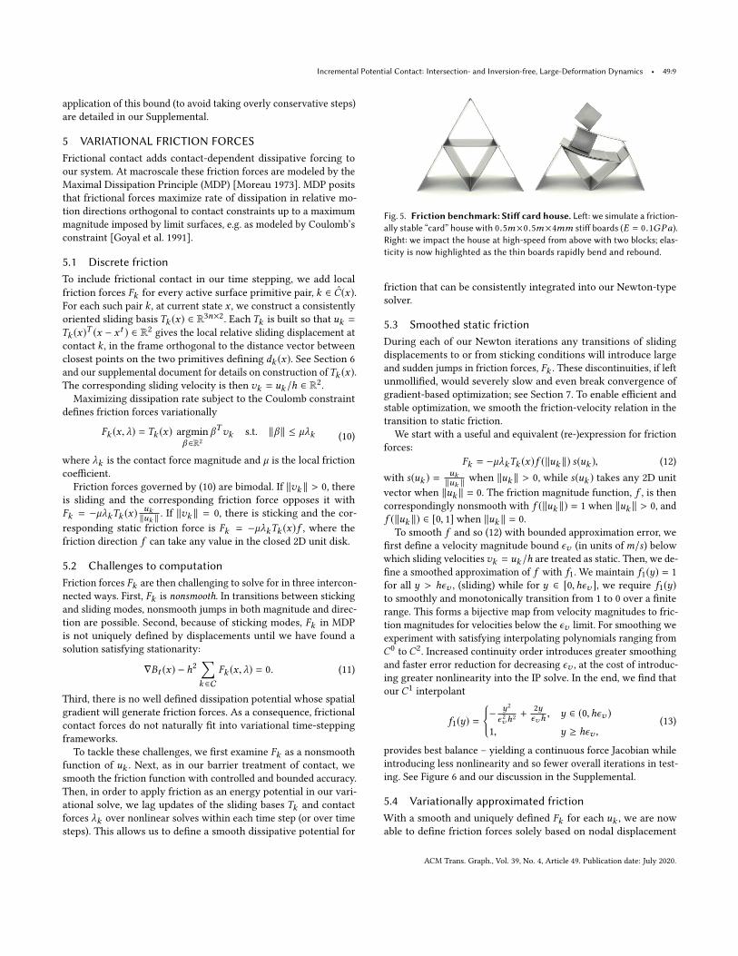
Fig. 5. Friction benchmark: Stiff card house. Left: we simulate a friction-
ally stable łcardž house with 0.5m×0.5m×4mm stiff boards (E = 0.1GPa).
Right: we impact the house at high-speed from above with two blocks; elas-
ticity is now highlighted as the thin boards rapidly bend and rebound.
friction that can be consistently integrated into our Newton-type
solver.
5.3 Smoothed static friction
During each of our Newton iterations any transitions of sliding
displacements to or from sticking conditions will introduce large
and sudden jumps in friction forces, Fk . These discontinuities, if left
unmollified, would severely slow and even break convergence of
gradient-based optimization; see Section 7. To enable efficient and
stable optimization, we smooth the friction-velocity relation in the
transition to static friction.
We start with a useful and equivalent (re-)expression for friction
forces:
Fk = −µλkTk (x)f (∥uk ∥) s(uk ), (12)
with s(uk ) =uk∥uk ∥
when ∥uk ∥ > 0, while s(uk ) takes any 2D unit
vector when ∥uk ∥ = 0. The friction magnitude function, f , is then
correspondingly nonsmooth with f (∥uk ∥) = 1 when ∥uk ∥ > 0, and
f (∥uk ∥) ∈ [0, 1] when ∥uk ∥ = 0.
To smooth f and so (12) with bounded approximation error, we
first define a velocity magnitude bound ϵv (in units ofm/s) below
which sliding velocitiesvk = uk/h are treated as static. Then, we de-
fine a smoothed approximation of f with f1. We maintain f1(y) = 1
for all y > hϵv , (sliding) while for y ∈ [0,hϵv ], we require f1(y)
to smoothly and monotonically transition from 1 to 0 over a finite
range. This forms a bijective map from velocity magnitudes to fric-
tion magnitudes for velocities below the ϵv limit. For smoothing we
experiment with satisfying interpolating polynomials ranging from
C0 to C2. Increased continuity order introduces greater smoothing
and faster error reduction for decreasing ϵv , at the cost of introduc-
ing greater nonlinearity into the IP solve. In the end, we find that
our C1 interpolant
f1(y) =
{
−y2
ϵ 2vh2 +
2yϵvh, y ∈ (0,hϵv )
1, y ≥ hϵv ,(13)
provides best balance ś yielding a continuous force Jacobian while
introducing less nonlinearity and so fewer overall iterations in test-
ing. See Figure 6 and our discussion in the Supplemental.
5.4 Variationally approximated friction
With a smooth and uniquely defined Fk for each uk , we are now
able to define friction forces solely based on nodal displacement
ACM Trans. Graph., Vol. 39, No. 4, Article 49. Publication date: July 2020.

49:10 • Minchen Li, Zachary Ferguson, Teseo Schneider, Timothy Langlois, Denis Zorin, Daniele Panozzo, Chenfanfu Jiang, and Danny M. Kaufman
-1 -0.5 0 0.5 1
Tangent relative velocity
-1
-0.5
0
0.5
1
Frictio
n f
orc
e
-1 -0.5 0 0.5 1
Tangent relative velocity
-1
-0.5
0
0.5
1
Friction forc
eFig. 6. Friction smoothing in 1D. Left: increasing orders of our polynomi-
als better approximate the friction-velocity relation with increasing smooth-
ness. Right: Our C1 construction improves approximation to the exact re-
lation as we make our frictional accuracy threshold, ϵv , and so the size of
static friction zone, smaller.
unknowns. A next natural step would then be to define a so-called
dissipative potential [Kane et al. 2000; Pandolfi et al. 2002] for in-
clusion in our optimization. An ideal potential would be a scalar
function with respect to x whose gradient returns Fk . However, even
with our smoothing, no well-defined displacement-based potential
for friction exists, and Fk cannot be approximated by a potential
force without introducing significant approximation errors. In other
words, we do not have a variational form of friction that we can yet
minimize.
We start by making dependence of our friction on bothTk (x) and
λk (x) explicit:
Fk (x, λk ,Tk ) = −µλkTk f1(| |uk | |)uk| |uk | |
. (14)
Now, if we setTk = Tk (x) and λk = λk (x) this friction evaluation is
exact. However, if we decouple dependence of the evaluated sliding
basis and contact force from x and instead lag them to values, λn,Tn ,
from a prior nonlinear solve (or previous time step) n, then all
remaining terms in the expression for friction are integrable. The
lagged friction force is then Fk (x, λnk,Tn
k) and provides a simple and
compact friction potential,
Dk (x) = µλnkf0(| |uk | |). (15)
Here f0 is given by the relations f ′0 = f1 and f0(ϵvh) = ϵvh so
that Fk (x) = −∇xDk (x). This potential provides easy-to-compute
Hessian, ∇2xDk (x), and energy contributions to the barrier potential,
described in detail in the supplemental document. Our full friction
potential is then D(x) = h2∑
k ∈C Dk (x), and the frictional barrier-
IP potential for the time step t + 1 is
Bt (x, d) + D(x). (16)
Friction Hessian projection. For our Newton method (Section 4.3),
we again need to project the friction potential Hessian to the space
of PSD matrices. The friction Hessian structure is similar to that of
elasticity, in that it can be written as a product of the Tk matrices.
This allows us to apply the same strategy as used for elasticity
Hessians, and so we need only perform a 2 × 2 PSD projection
for each friction term per primitive pair. This is detailed in our
Supplemental.
5.5 Frictional contact accuracy
Accuracy of friction forces generated by each solution of our IP (16)
are defined by the static threshold, sliding basis and contact force
magnitudes.
Static friction threshold. As we apply smaller ϵv we decrease the
range of sliding velocities that we exert static friction upon and
correspondingly sharpen the friction forces towards the exact non-
smooth friction relation. Decreasing ϵv thus reduces stiction error
while increasing compute times as we introduce a sharper nonlin-
earity in a tighter range; see Figure 6. For accurate reproduction
of dynamic behaviors with friction and for visually plausible re-
sults, we observed that ϵv = 10−3ℓm/s , where ℓ is characteristic
length (i.e. bounding box size), works well as a default across a wide
range of examples with friction coefficients. See e.g., Figure 8. As
static accuracy becomes important, we then find solutions with
ϵv = 10−5m/s work well. We have further confirmed IPC conver-
gence down to ϵv = 10−9m/s . See, for example, our reproduction
of the stable frictional contact structures in the masonry arch and
card house examples in Figures 5 and 7.
Friction direction and magnitude. We improve accuracy of the
direction and magnitude of the friction forces by solving successive
minimizations of (16) within each time step. For each solve we
update the lagged Tn and λn (warm-starting from the previous
time step) with results from the last nonlinear solve. Convergence
of lagged iterations is then achieved when we reach approximate
momentum balance with
∥∇Bt (xt+1) − h2
∑
k ∈C
Fk (xt+1, λt+1,T t+1)∥ ≤ ϵd , (17)
where ϵd is the targeted dynamics accuracy.
We confirm lagged iterations rapidly converge over nonlinear
solves with our FE models for the well-known, standard frictional
benchmarks, e.g., block-slopes, catenary arches and card houses.
See Figures 7 and 5 and Section 7. However, we emphasize that we
do not have convergence guarantees for lagging. In particular, we
have identified cases with large deformation and/or high speed im-
pacts where we do not reach convergence forT and λ in the friction
Fig. 7. Friction benchmark:Masonry arch. IPC captures the static stable
equilibrium of a 20m high cement (ρ = 2300kд/m3, E = 20GPa, ν = 0.2)
arch with tight geometric, d = 1µm, and friction, ϵv = 10−5m/s accuracy.
Decreasing µ then obtains the expected instability and the stable arch
does not form (see our supplemental videos). Inset: zoomed 100× (orange)
highlights the minimal gaps with a geometric accuracy of small d .
ACM Trans. Graph., Vol. 39, No. 4, Article 49. Publication date: July 2020.

Incremental Potential Contact: Intersection- and Inversion-free, Large-Deformation Dynamics • 49:11
Fig. 8. Large deformation, frictional contact test. We drop a soft ball
(E = 104Pa) on a roller (made transparent to highlight friction-driven
deformation). Here IPC simulates the ball’s pull through the rollers with
extreme compression and large friction (µ = 0.5).
forces. Thus, in our large-deformation frictional examples we apply
just a single lagging iteration. In these cases, sliding directions and
contact force magnitudes in the friction force evaluation may not
match. However, even in these cases, all other guarantees, including
non-intersection, momentum balance (as in the frictionless case)
and accurate stiction are maintained. More generally, we observe
high-quality, predictive frictional results for large deformation ex-
amples independent of the number of lagging iterations applied; see
e.g. Figure 16. We also emphasize that for frictionless models, IPC
continues to guarantee convergence for contact and elasticity with
just a single nonlinear solve per time step.
6 DISTANCE COMPUTATION
Evaluating unsigned distance functions between point-triangle and
edge-edge pairs requires care as closed-form distance formulas
change with relative position of surface primitives.
6.1 Combinatorial distance computation
Unsigned distances are given by the closest points on the two prim-
itives evaluated.
Distance between a point vP and a triangle T = (vT 1,vT 2,vT 3)
can be formulated as a constrained optimization problem,
DPT=minβ1,β2| |vP − (vT 1 + β1(vT 2 −vT 1) + β2(vT 3 −vT 1))| |
s .t . β1 ≥ 0, β2 ≥ 0, β1 + β2 ≤ 1.(18)
Similarly the distance between edges v11-v12 and v21-v22 is
DEE=minγ1,γ2| |v11 + γ1(v12 −v11) − (v21 + γ2(v22 −v21))| |
s .t . 0 ≤ γ1,γ2 ≤ 1.(19)
Each possible active set of these two minimizations corresponds to a
closed-form distance formula. In each, at most two constraints can
be active at the same time.
• When two constraints are active in either (18) or (19), the distance
between primitives is a point-point distance evaluation:
dPP = | |va −vb | |. (20)
Here va and vb correspond to vP and a vT i for (18), or to the two
endpoints of the edges in the edge-edge pair for (19).
• When a single constraint is active in either (18) or (19), the distance
in both cases becomes a point-edge distance evaluation:
dPE =| |(va −vc ) × (vb −vc )| |
| |va −vb | |. (21)
Here (va,vb ) corresponds to one of the triangle edges of T and
vc = vP for (18), or else (va,vb ) corresponds to one of the edges
in the edge-edge pair and vc corresponds to an endpoint of the
other edge for (19).
• When no constraints are active in either (18) or (19), distance
computations are simply parallel-plane distance evaluations. For
the point-triangle pairing in (18) this is
dPT = |(vP −vT 1) ·(vT 2 −vT 1) × (vT 3 −vT 1)
| |(vT 2 −vT 1) × (vT 3 −vT 1)| ||, (22)
while for the edge-edge pairing in (19) it is
dEE = |(v11 −v21) ·(v12 −v11) × (v22 −v21)
| |(v12 −v11) × (v22 −v21)| ||. (23)
For evaluations of d , ∇d , and ∇2d , we apply the currently valid,
closed-form distance formula (either PP, PE, PT, or EE above) and
its analytic derivatives. The formula to apply, at each evaluation of
a surface pair, is determined by the active constraint subset defined
by the current relative positions of the pair’s primitives. This infor-
mation is computed and stored together with our culled constraint
set C data, and so is then available for direct use whenever comput-
ing barrier energies and derivatives. This treatment is analogous to
storing and reusing singular value decompositions of deformation
gradients for elasticity computations. As in elasticity, our distance
state and evaluations can efficiently be reused for all energy and
derivative evaluations at the same nodal positions. Correspondingly,
having now reduced general point-triangle and edge-edge distance
evaluations to the above closed-form formulas, we can directly com-
pute and store our sliding bases, Tk (x), for friction computation
with respect to each case; please see our Supplemental for details.
6.2 Differentiabilty of d
A B
C D
A B
C D
∇dA
∇dB
∇dA
∇dB
∇dC ∇d
D= 0 ∇d
C= 0 ∇d
D
(a) (b)
Fig. 9. Nonsmoothness of parallel
edge-edge distance.When edgeAB
andCD are parallel, the distance com-
putation can be reduced to either (a)
C−AB point-edge or (b)D−AB point-
edge. Then for the trajectory ofC mov-
ing down from above D , the distance
gradient is not continuous at the par-
allel point even though the distance
is always continuously varying.
In collision-resolutionmeth-
ods, close-to-parallel edge-
edge contacts are notori-
ous failure modes ś to the
extent that existing meth-
ods often ignore this case
by throwing out all corre-
sponding constraints [Har-
mon et al. 2008]. How-
ever, despite the challenges
imposed, these constraint
cases cannot be removed,
as doing so would lead to
intersection. The reason for
the difficulty in these cases
is the (lack of) differentia-
bility of the distance func-
tion for some configurations. Each above analytic formula for dis-
tances corresponds to a subset of the relative configuration space of
ACM Trans. Graph., Vol. 39, No. 4, Article 49. Publication date: July 2020.

49:12 • Minchen Li, Zachary Ferguson, Teseo Schneider, Timothy Langlois, Denis Zorin, Daniele Panozzo, Chenfanfu Jiang, and Danny M. Kaufman
a primitive pair. For example, for vertex-triangle pairs, relative con-
figurations are completely characterized by fixing the triangle and
varying vP positions. If the projection of vP to T is in the triangle
interior, no constraints are active, while if the projection lies on the
interior of a triangle edge then one constraint is active. Otherwise,
two constraints are active.
Each of these geometric criteria defines a subset of R3, where one
of the three analytic formulas is valid. The distance function is C∞
inside each such domain, and, in general, is C1 at the boundaries
between domains. However, the critical exception is in parallel edge-
edge configurations: at these points, the distance function is not
differentiable (see Figure 9). Configurations close to these parallel
edge-edge conditions, when reached, lead to unacceptably slow
convergence of Newton iterations or even convergence failures
altogether. Numerically, the issue is similar to the C0-continuous
friction problem we faced in Section 5.2. To resolve this issue, we
once again apply a local smoothing solution to mollify the barrier
corresponding to nearly parallel edge-edge contact conditions.
We smooth bymultiplying all edge-edge barrier terms by a piecewise-
polynomialmollifier closely analogous to our static-friction smoother;
recall Figure 6. Here, for each edge-edge contact pair k , we define
ek (x) to vanish when edges (v11v12 − v21v22) are parallel and to
smoothly grow to 1 as the edge-pair become far from parallel,
ek (x) =
{
− 1ϵ 2×c2 + 2
ϵ×c c < ϵ×,
1 c ≥ ϵ×,(24)
where c = | |(v12 − v11) × (v22 − v21)| |2 and ϵ× = 10−3 | |v ′12 −
v ′11 | |2 | |v ′22 −v
′21 | |
2 is defined with respect to edge-edge vertex-pair
rest positions v ′.
Our mollified edge-edge barriers are then ek (x)b(
dk (x))
and so
now extend our barrier potentials to a piecewiseC∞, everywhereC1-
continuous (for nonintersecting configurations) barrier formulation.
At the same time our barriers now remain sufficient to guarantee
that no collisions are missed: there are always point-triangle contact
pairs at distance no more than the parallel edge-edge distance; see
our Supplemental for details on this. In turn, our construction of the
parallel-edge mollifier then minimizes its impact on edge-edge pair
barriers as they move away from degeneracy. While in principle
increasing smoothness to C1 is sufficient to avoid most dramatic
degeneracy failures, there are additional numerical stability issues
to be addressed related to nearly parallel edges. Please see our
Supplemental for details.
Now, with this third and last smoothing in place we have an
overall time-stepping potential for contact and friction that can
leverage superlinear convergence and robustness of Newton-type
stepping. As we analyze in Sections 7 and 8 below (see especially 7.1)
this gains robust simulation against failure ś even when simulating
challenging conditions with unavoidable numbers of degenerate
evaluations.
7 EVALUATION
Our IPC code is implemented in C++, parallelizing assembly and
evaluations with Intel TBB, applying CHOLMOD [Chen et al. 2008]
with AMD reordering for linear system solves in all examples (with
the exception of the squishy ball example ś see below) and Eigen
[Guennebaud et al. 2010] for linear algebra routines. We run most
experiments on a 4-core 3.5GHz Intel Core i7, a 4-core 2.9 GHz
Intel Core i7, and a 8-core 3.0 GHz Intel Xeon machine. Machine
use per example is summarized along with performance statistics
and problem parameters in Figure 23 and in our Supplemental. The
reference implementation, scripts used to generate these results and
our benchmarks are released as an open-source project.
Linear system computations and solves. We compute elasticity
and barrier Hessians (with PSD projections) in parallel, and have
designed and implemented a custom multi-threaded, sparse ma-
trix data structure construction routine that, given the connectivity
graph of nodes, efficiently builds the CSR format with index entries
ready. While we utilize efficient symbolic factorization and parallel
numerical factorization routines in CHOLMOD [Chen et al. 2008]
compiled with MKL LAPACK and BLAS, we also tested IPC with
AMGCL [Demidov 2019] ś a multigrid preconditioned solver. Here,
we found behavior is as might be expected, less memory overhead
and faster linear solves by avoiding direct factorization. However,
for majority of examples the large deformations and many contacts
generate poorly conditioned systems. We then found AMGCL re-
quires extensive parameter tuning to perform well and still can not
compete, in general, with the parallel direct solver. All examples
in the following then apply CHOLMOD for linear solves, with the
exception of our largest, squishy ball example (Figure 22), where
we apply AMGCL.
Models and practical considerations. We primarily employ the non-
inverting, neo-Hookean (NH) elasticity model and implicit Euler
time stepping. In the following examples we also apply and evalu-
ate implicit Newmark time stepping, as well as the invertible fixed
corotational elasticity (FCR) elasticity model. While for clarity in
the preceding we derive IPC with unmodified distance evaluations,
for numerical accuracy and efficiency our implementation applies
squared distances for evaluations of the barrier, we use b(d2, d2),
and related computations, thus avoiding squared roots. In turn ex-
pressions for contact forces, λk , and related terms must be modified,
from our direct exposition and derivations above. To do sowe rescale
for consistent dimensions and units in our implementation; see our
Supplemental for details. Finally and importantly we note that IPC’s
barrier formulation requires nonzero separation distances to be
strictly satisfied at initialization and then guarantees it throughout
simulation. Exact initialization at zero distance is neither possible (as
the barrier of course diverges) nor for that matter physically mean-
ingful. Contact, including resting contact, instead occurs around
the specified geometric distance accuracy given by the user. Here
we demonstrate simulated configurations with distances down to
10−8m reached in simulation (e.g. arch in Figure 7) or initialized by
users.
Evaluation and tests. Below we first introduce a set of unit tests
for seemingly simple yet challenging scenarios with nonsmooth,
aligned and close contacts (Section 7.1), stress tests involving large
deformation and high velocities (Section 7.2), and friction (Section
7.3). We next study IPC ’s scaling, run time, and accuracy behavior
as we vary simulation problem parameters (Section 7.4). Finally, we
ACM Trans. Graph., Vol. 39, No. 4, Article 49. Publication date: July 2020.

Incremental Potential Contact: Intersection- and Inversion-free, Large-Deformation Dynamics • 49:13
present an extensive, quantitative comparison with previous works
in Section 8.
7.1 Unit tests
Fig. 10. Aligned, close and nonsmooth contact tests. Pairs of before
and after frames of deformable geometries initialized with exact alignment
of corners and/or asperities; dropped under gravity. We confirm both non-
smooth and conforming collisions are accurately and stably resolved.
Aligned, close and nonsmooth contact. We apply a set of unit
tests exercising closely aligned, conforming and nonsmooth contact
known to stress contact algorithms. We build them with two simple
models: a single tetrahedron and an 8-node unit cube; see Figure
10 and Figures 11. For contact handling, these seemingly simple
tests are designed to trigger degenerate edge cases that often cause
failure in existing methods (see Section 8). IPC resolves all cases
including those in which we exercise exact parallel edge-edge (e.g.,
Figure 10 middle) and point-point (e.g., Figure 10, left) collisions. For
unit tests like Figure 10 right we drop objects into slotted obstacles
so that they fit tightly with tiny gaps; here IPC retrieves a tight
conforming fit into a 1µm gap.
Fig. 11. Erleben tests Top: fundamental test cases to challenge mesh-based
collision handling algorithms proposed by Erleben [2018]. Bottom: IPC
robustly passes all these tests even when stepped at frame-rate size time
steps.
Erleben fundamental cases. Erleben [2018] proposes unit tests
(see Figure 11 top row) for contact constraint failure testing. Here
these tests are again simple but designed to challenge mesh-based
collision-handling algorithms. IPC again resolves all tests robustly
(see Figure 11, bottom row), even when stepped at frame-rate size
time steps.
Tunneling. Tunneling through obstacles when simulating high-
speed velocities is a common failure mode in dynamic contact mod-
eling. We thus add an example to our unit tests: we fire an elastic
ball (diameter 0.1m) at a fixed 0.02m thin board at successive speeds
of 10m/s, 100m/s, and 1000m/s stepped at h = 0.02s . IPC accurately
rebounds at large time step without tunneling in all cases.
Fig. 12. Large Mass and Stiffness ratios.
Large mass and stiffness ratio tests. Contact resolution between
objects with largely varying scale, mass, and/or stiffness ratios has
long-challenged time stepping methods due to ill-conditioning. In
Figure 12, we simulate IPC dropping of a range of objects upon
each other with widely varying weight and stiffness. Here we apply
E = 0.1GPa for the sphere, board, and large cube, E = 1MPa for the
small cube and the mat holding the sphere, and E = 10KPa for the
mat dropped on boards. For the stiff ball and large cube, we set their
respective densities to 2× and 10× that of softer objects (1000kд/m3)
to add large mass ratios to the challenge. Regardless of these differ-
ent ill-conditioned settings, IPC simulates all scenes robustly and
efficiently without any artifacts; see also our supplemental videos.
Chains. While resolving transient collisions exercises stability,
large numbers of persistent, coupled contacts, as in a long chain of
elastic links, exercises contact constraint accuracy. A small amount
of constraint error integrated over time will cause such chains to
break. We simulate chains of 100 elastic links under gravity, observe
stable oscillations and shock-propagation while shorter chains sta-
bly bounce ś all preserve constraints; see our supplemental videos.
7.2 Stress tests
We next consider IPC’s ability to resolve a range of extreme stress-
test examples motivated by well-known pre-existing challenges and
previously proposed benchmarks.
Funnel. To confirm contact resolution under strong boundary
conditions, extreme compression, and elongation, we pull a stiff
NH material dolphin model through a codimensional funnel mesh
obstacle. We step IPC at large time steps of h = 0.04s with up to
32.3K contacts per step. The resulting simulation is intersection-
and inversion-free throughout with the model regaining its rest
shape once pulled through (Figure 13).
Thin volumetric meshes. Thin geometries notoriously stress con-
tact simulations. Likewise, as more simulation nodes are involved
in collision stencils, simulation challenges grow. Here we test IPC’s
handling of extreme cases with both challenges, by simulating single
layer meshes of tetrahedra. Here IPC robustly handles the contacts
with accurate solutions at all time steps across a range of large
deformation contact examples (Figures 5, 12 and 14).
ACM Trans. Graph., Vol. 39, No. 4, Article 49. Publication date: July 2020.

49:14 • Minchen Li, Zachary Ferguson, Teseo Schneider, Timothy Langlois, Denis Zorin, Daniele Panozzo, Chenfanfu Jiang, and Danny M. Kaufman
funnel
Fig. 13. Funnel test. Top: the tip of a stiff neo-Hookean dolphin model
is dragged through a long, tight funnel (a codimensional mesh obstacle).
Middle top: due to material stiffness and tightness of fit the tip of the model
is elongated well before the tail pulls through. Middle bottom: extremity of
the deformation is highlighted as we zoom out immediately after the model
passes through the funnel. Bottom: finally, soon after pulling through, the
dolphin safely recovers its rest shape. We confirm that the simulation is
both intersection- and inversion-free throughout all time steps.
Fig. 14. Stress test: extreme twisting of a volumetricmat for 100s. Left:
IPC simulation at 10s after 2 rounds of twisting at both ends. Right: at 40s
after 8 rounds of twisting. This model, designed to stress IPC, has all of its
45K simulation nodes lying on the mesh surface.
Extreme and extended twisting. As large deformation high-contact
examples, we twist thin mats (Figure 14), rods (Figure 4), and Ar-
madillos (Figure 21, bottom) with rotating speeds of 72◦/s at both
ends. We simulate the twist of both the rods and mats for 100s
ś efficiently capturing increasingly tight conforming contact and
expected buckling in all simulations.
Compactor test. In Figure 15 we test łtrashž compactor-type exam-
ples from Harmon et al. [2009]. After releasing the compactor from
the extreme compression point we clearly see that the tentacles of
the octocat model and correspondingly the sphere, mat, and bunnies
models are all cleanly separated.
Rollers compression and stick-slip instability. To combine extreme
deformation with friction, we match the set-up of the kinematic
roller test from Vershoor and Jalba [2019] with the same originally
applied, high friction coefficient µ = 0.5 (Figure 16). This scene is
highly challenging due to the competing large magnitude of the
friction and the large compression induced by the rollers. Here,
Fig. 15. Trash Compactor. An octocat (left) and a collection of models
(right) are compressed to a small cube by 6 moving walls and then released.
Here, under extreme compression IPC remains able to preserve intersection-
and inversion- free trajectories solved to requested accuracies.
Fig. 16. Roller tests. Simulating the Armadillo roller from Verschoor and
Jalba [2019] (same material parameters) in IPC now captures the expected
stick-slip behavior for the high-friction, moderate stiffness conditions.
with a moderately stiff material (E = 5 × 10⁵Pa Young’s modulus)
we observe that IPC with our friction model obtains the expected
stick-slip instability effects that such competition should generate.
In simulation we observe deformation grows in opposition to static
friction in the rollers until stress overcomes static friction and we
observe slip ś this process is then repeated. This stick-slip effect is
captured by our Armadillo with moderate stiffness when tested with
both the NH and FCR elasticity models (see our supplemental videos
for the motion). We also note, as expected, when we subsequently
test with softer material, i.e., E = 105Pa, we get smooth rolling
behavior for the Armadillo, as expected, without stick slip.
Fig. 17. Codimensional collision objects: pin-cushions We drop a soft
ball onto pins composed of codimensional line-segments and then torture it
further by pressing downwith another set of codimensional pins to compress
from above. IPC robustly simulates the ball to a łsafež, stable resting state
under compression against the pins.
Codimensional collision obstacles. Collision obstacles, especially
in animation and gaming, are often most easily expressed in their
default form as triangle meshes or even unorganized triangle soups.
While highly desirable in applications, codimensional collision types
are not generally supported by available simulation methods, which
ACM Trans. Graph., Vol. 39, No. 4, Article 49. Publication date: July 2020.

Incremental Potential Contact: Intersection- and Inversion-free, Large-Deformation Dynamics • 49:15
often suffer tunneling, snagging, and resulting instabilities when ex-
posed to them. To our knowledge IPC is the first algorithm to stably
and accurately resolve collisions between volumes and codimen-
sional collision objects. We perform a set of tests dropping different
objects on planes, segments, and points, see e.g. Figures 2, 17 and
18. Collisions are stably resolved and we see tight compliance to the
sharp poking obstacles in contacting regions.
Fig. 18. Codimensional collision objects: rollers We modify the ball
roller example from Figure 8 by using only the edge segments (left) or
even just vertices (right) for the moving roller obstacle. For these extremely
challenging tests IPC continues robust simulation exhibiting tight compliant
shapes in contact regions pressed by the sharp obstacles.
Codimensional rollers. What if we modify the roller test in Figure
8, leaving only the edges or even only the points for the roller
obstacles? This leads to our codimensional roller tests (Figure 18).
Here, with solely codimensional wire (just edges) and points (just
vertices) rollers, the big ball still pulls inwards, forming tightly
pressed geometries in the contact regions as it is compressed and
pulled against and then out of the codimensional rollers (Figure 18).
For sharp point rollers we require negligible friction (for points we
apply µ = 10−3) to pull the ball inwards as the sharp points directly
grab the deforming surface.
Squeeze out stress test. A plate compresses and then forces a col-
lection of complex soft material models into a tight conforming
mush through a thin co-dimensional tube obstacle. Once through
they cleanly separate (Figure 1).
High speed impact test. To examine IPC’s fidelity in capturing
high-speed dynamics we match the reported material properties
and firing speed of an experiment of foam practice ball fired at
high-speed towards a fixed steel wall. In Figure 19 top, we show key
frames of a high-speed capture of the event. Middle: we visualize ve-
locity magnitudes simulated by IPC , stepped with implicit Newmark
and the NH material, at the same corresponding times in the simula-
tion, and bottom the IPC-simulated geometry. Here we observe both
the expected shockwave propagating through the sphere during
the finite-time collision as well as the overall matching dynamics
and shape across the simulation. Please see our supplemental video
for complete simulation moving through the phases of inelastic
collision impact: compression (first shockwave), restoration (second
shockwave), and release.
7.3 Frictional contact tests
To examine IPC’s frictional model we simulate a set of increasingly
challenging frictional benchmark tests. All utilize a tight accuracy
of ϵv = 10−5m/s and apply lagged iterations to update sliding bases
video footage
simulation
velocity
magnitude (m/s)0 m/s
67 m/s
0 67
Fig. 19. High-speed impact test. Top: we show key frames from a high-
speed video capture of a foam practice ball fired at a fixed plate. Matching
reported material properties (0.04m diameter, E = 107Pa, ν = 0.45, ρ =
1150kg/m3) and firing speed (v0 = 67m/s), we apply IPC to simulate the
set-up with Newmark time stepping at h = 2 × 10⁻⁵s to capture the high-
frequency behaviors. Middle and bottom: IPC-simulated frames at times
corresponding to the video frames showing respectively, visualization of the
simulated velocity magnitudes (middle) and geometry (bottom).
Fig. 20. Stick-slip oscillations with friction simulated with IPC by dragging
an elastic rod along a surface.
and normal forces until the system is confirmed as fully converged
by satisfying (11).
Block tests. We start by placing stiff elastic blocks on a slope
with tangent at 0.5. Here for µ = 0.5, IPC generates the expected
result of frictional equilibrium ś the block does not slide. Switching
to µ = 0.49, IPC then immediately sets the block sliding, again
matching the analytic solution.
Frictionally dependent structures. We test IPC on the challenging,
frictionally dependent stable structure tests from Kaufman et al.
[Kaufman et al. 2008]. We model both the card house (Figure 5) and
masonry arch (Figure 7) with stiff deformable materials. We further
extend the challenge of the arch with a precarious base balanced
on sharp edges. We obtain long-term stable structures with µ = 0.5
and µ = 0.2 respectively and confirm that they fall apart as we
reduce to µ = 0.2 and µ = 0.1 respectively (see our supplementals
for statistics and videos).
ACM Trans. Graph., Vol. 39, No. 4, Article 49. Publication date: July 2020.

49:16 • Minchen Li, Zachary Ferguson, Teseo Schneider, Timothy Langlois, Denis Zorin, Daniele Panozzo, Chenfanfu Jiang, and Danny M. Kaufman
Table 1. Increasing time step sizes to frame-rate and beyond.Here we
demonstrate tradeoffs in varying time step sizes for the same tight twisted
rods example (2.5K nodes, 6.9K tets, 4.6K faces, E = 104Pa) with a 4-core
2.9GHz Intel Core i7 CPU, 16GB memory. # iters is the number of Newton
iterations per time step or in total for the simulation sequences.
h (s)# constraints
avg (max)
per time step total
t (s) # iters t (s) # iters
0.002 137 (430) 0.29 2.12 862 6351
0.005 194 (584) 0.36 2.37 435 2843
0.01 269 (707) 0.38 2.65 229 1591
0.025 435 (1.0K) 0.38 2.69 91 645
0.05 551 (1.2K) 0.46 3.06 56 368
0.1 597 (1.3K) 0.73 4.75 44 285
0.2 607 (1.2K) 1.79 14.37 54 431
0.5 653 (1.4K) 11.39 100.58 137 1207
1 708 (1.3K) 18.41 188.17 110 1129
2 843 (1.3K) 52.02 522.00 156 1566
Stick-slip instability. Finally, we script the motion of the top of a
thin, volumetric elastic rod pushed slightly down towards, and then
along a surface (µ = 0.35) to test stick-slip oscillations. As in the
Armadillo roller example, large static friction creates a buildup of
elastic energy in the rod which is released when the friction force,
opposing sliding contact, is exceeded by the tangential stiffness
at the contact. This interaction between the friction forces and
the sliding velocities becomes periodic, and so induces self-excited
oscillations that buildup and dissipate energy; see Figure 20 and our
supplemental video.
7.4 Scaling, Performance, and Accuracy
Varying time step sizes. Existing contact-resolution methods gen-
erally rely on small time step sizes for simulation success. As demon-
strated above, IPC is able to simulate across a wide range of time
step sizes h and so can capture a range of different frequency effects.
Choice of time step size for IPC is then simply a question of accu-
racy required per application as balanced against efficiency needed,
rather than a predicate required for success. To investigate the effect
of varying time step size,h, in IPC we simulate the tight twisted rods
example (Figure 4) for 6s. We range h from 0.002s to 2s . In Table 1
we observe that transitioning from large to small time step sizes, our
method improves its per time-step performance ś but not by orders
of magnitude. This is because the costs of intersection-free time
stepping, distance computation and CCD do not change much. Since
we do not miss any contacts, the number of constraints we process
decrease only sublinearly as we decrease time step sizes. This is
a key computational feature to ensure feasibility and robustness.
On the other hand, we happily observe that our method is robust
even well beyond standard time step sizes. While, in general, such
excessively large step sizes beyond frame-rate are not useful for
dynamics, this offers a robust opportunity for quasi-statically com-
puting equilibria subject to challenging contact conditions. When
we deploy IPC with implicit Euler IP (taking advantage of numerical
dissipation), these very-large time steps rapidly compute equilibria
with extreme contact conditions in just a few steps.
0 1 2 3
# nodes 105
0
50
100
150
tim
e (
s)
0 1 2 3
# nodes 105
0
2000
4000
6000
8000
me
mo
ry (
MB
)
Fig. 21. Scaling tests. Top: applying increasing resolution meshes ranging
from 3K to 219K nodes we examine the time (left) and memory (right)
scaling behavior of IPC on a range of resolutions of the twisting Armadillo
and twisting mat (Figure 14) examples. Bottom: frames from the highest-
resolution twisting Armadillo example (219K nodes, 928K tets).
Scaling. In Figure 21 top, we study scaling behavior of IPC , with
twisting mat (Figure 14) and twisting Armadillo (Figure 21, bottom)
simulations of increasing-resolution meshes ranging from 3K to
219K nodes. Armadillo is a representative volumetric model while
the single-layer mat is an extreme example designed to especially
stress IPC . The mat meshes importantly have all simulation nodes
on their surfaces and so, as contacts tighten in the twisting mat, they
can form arbitrarily dense Hessians. For themat we observe iteration
count, memory and contact counts increase linearly with resolution,
while timing increases in a slight superlinear trend. For the more
standard volumetric Armadillo model we observe iteration count
remains flat as we increase resolution, while timing and memory
increase linearly.
In addition, when mesh sizes and contacts grow large, available
memory can potentially preclude application of direct linear solvers.
To confirm IPC applicability in these settings we simulate the firing
of a 688K node, 2.3M tetrahedra, squishy ball model from Zheng
and James [2012] at a glass board using AMGCL’s [Demidov 2019]
multigrid-preconditioned iterative linear solver. Here both the large
element count and the large numbers of collisions enabled by the
toy’s many colliding tendrils introduce very large system solves
during the most contact-rich steps colliding against the glass (Figure
22).
Performance. Comprehensive statistics on all simulations, models,
parameters and performance are reported in Table 23 and in our
Supplemental. For reference dynamics please see our supplemental
videos.
Accuracy. User-facing parameters in IPC have three accuracies
that can be specified: 1) dynamics accuracy (ϵd ), defining how well
dynamics are resolved; 2) geometric accuracy (d), defining how close
objects can come to touching; and 3) stiction accuracy (ϵv ), defining
howwell static friction is resolved. All three provide users direct and
intuitive control (with meaningful physical units) of the trade-off
between accuracy and compute cost.
ACM Trans. Graph., Vol. 39, No. 4, Article 49. Publication date: July 2020.

Incremental Potential Contact: Intersection- and Inversion-free, Large-Deformation Dynamics • 49:17
Fig. 22. Squishy ball test: Simulated by IPC an elastic squishy ball toy
model (688K nodes, 2.3M tets) is thrown at a glass wall. The left three frames
show side views before, at, and after the moment of maximal compression
during impact. The right-most frame then shows the view behind the glass
during the moment of maximal compression, highlighting how all of the
toy’s intricately intertwined tendrils remain intersection free.
In our extensive testing, IPC converges to satisfy these requested
accuracies while always maintaining an intersection- and inversion-
free state. These guarantees (non-intersection, non-inversion) hold
even as we radically increase speed of collision at large time step,
apply extreme deformations, and model highly stiff materials. We
have tested this across a wide range of test examples with material
stiffnesses up to E = 2 × 10¹¹Pa and have confirmed our IPC im-
plementation’s ability to converge to tight tolerances for all these
measures when requested with ϵd down to 10−7m/s, ϵv down to
10−8m/s , and d down to 1µm.
As we discuss and demonstrate in Sections 3 and 8, all previously
available methods introduce computational error for these accuracy
measures; to our knowledge, IPC is the first to provide and expose
direct and separable control of them. Our singular exception, as
detailed in Section 5 above, is the number of frictional lagging
iterations applied. When accurate friction is required, e.g., our arch,
stick-slip and card house experiments, we set no upper bound on
this parameter. Then as discussed above, in these examples IPC
fully converges and is entirely parameter-free. However, (as detailed
above) we do not have convergence guarantees for lagging, and in
our large-deformation frictional examples we apply a single lagging
iteration. In these cases, as discussed in Section 5.5, sliding directions
and contact forces in the friction may not match. However, even
in such cases all other guarantees, including non-intersection are
maintained. We observe high-quality results regardless of number
of lagging iterations applied or accuracies specified.
Finally, on the other end of the spectrum in many applications, e.g.
animation, it can be desirable to trade accuracy for efficiency. We
confirm robust, plausible behavior for IPC when we set very large,
loose tolerances on all the above parameters, e.g. with ϵd = 10−1m/s,
while still maintaining feasible (non-inverting, non-intersecting)
trajectory guarantees.
Exact CCD admissibility check. IPC’s collision aware line search
ensures intersection-free trajectories. Our implementation applies
standard floating-point CCD2 combined with the conservative ad-
vancement strategies detailed in Section 4 and our Supplemental
to ensure efficient, intersection-free stepping. Exact CCD then of-
fers the possibility for aggressive advancement of intersection-free
steps and so improved efficiency. To this end we tested the robust
2https://github.com/evouga/collisiondetection
CCD methods from both Bridson et al. [2002] and Tang et al. [2014]
but found the reference implementations for each missed critical
intersections in degeneracies. We then reimplemented Bridson et al.
[2002] with rationals. While this version now guarantees exactness,
it is much slower (∼30x) than our floating-point implementation.
Currently we apply this exact CCD just for re-analysis as a post step
check after every Newton iterate to test three of our challenging
contact stress tests: octocat on codimensional łknivesž, ball roller
and mat twist. We confirm that every step taken in every time step
was intersection free in these examples.
Varyingmaterial model. Ageneral expectation fromunconstrained
simulation is that modeling with non-invertible materials like NH
should be more costly than comparable set-ups with invertible ma-
terials like FCR. However, when studying our large deformation
examples with contact we find that the picture is more complex.
Here the larger bottleneck is generally resolving contact barrier
terms. In many examples we then observe that simulations with
NH and FCR have comparable cost. In a number of other simula-
tions with extreme contact conditions (e.g. pin-cushion and mat
twist) element degeneracies allowed by FCR actually increase over-
all cost of simulation well over the same simulations with the NH
material. Finally, in other cases where stress is most extreme (e.g.
armadillo roller and dolphin funnel), NH entails more cost than the
comparable simulation with FCR.
8 COMPARISONS
We perform extensive quantitative comparisons with existing al-
gorithms and commercial codes used in both computer graphics
(Section 8.1) and mechanical engineering (Section 8.2). Then, to
more fairly compare across a large class of previous contacts algo-
rithms based on SQP-type methods, we implement their core contact
resolution procedures in a single framework, and perform a large
scale comparison on our benchmark test set (Section 8.3). While our
implementations are not finely tuned as for the first two sets of com-
parisons, this approach allows us to compare the core algorithmic
components in a common, objective and unbiased context.
8.1 Computer Graphics Comparisons
Contact algorithms in graphics often target performance with small
compute budgets and so admirably face many efficiency challenges
in balancing fidelity against speed. We investigate what happens
if we push these methods’ settings to be most accurate without
regard to speed, e.g., max iteration caps of 1M per step and time
steps down to 10−5s . Here, nevertheless, we still document failures,
e.g., tunneling, non-convergence, instabilities and ghost forces, even
on very simple test examples.
Verschoor and Jalba [2019]. We apply the reference implementa-
tion [Verschoor and Jalba 2019] to reproduce available scenes from
Verschoor and Jalba with their default and reported input param-
eters. Here we observe that small adjustments to time step sizes
and material parameters lead to divergent simulations. Specifically,
the Armadillo roller example does not converge when applying
the implementation’s default time step of h = 10−3 for a range of
stiffnesses of E = 5× 10⁴, 5× 10⁵, and 5× 10⁶Pa, nor when applying
ACM Trans. Graph., Vol. 39, No. 4, Article 49. Publication date: July 2020.

49:18 • Minchen Li, Zachary Ferguson, Teseo Schneider, Timothy Langlois, Denis Zorin, Daniele Panozzo, Chenfanfu Jiang, and Danny M. Kaufman
the default material setting E = 5 × 10⁵Pa for a range of time step
sizes of h = 10−3, 2× 10⁻³, 4× 10⁻³, and 10−2s. In all these cases the
implementation maxes out at its default max-iteration cap of 1M.
We extract the Armadillo mesh, roller models and replicate the
same example in IPC with identical scene settings. Here it is note-
worthy that IPC applies fully nonlinear NH and FCR models with
variational friction while the reference code (matching paper) lin-
earizes elasticity once per time step. As covered in Section 7.2, IPC
obtains the stick-slip oscillations expected in this setting (see also
our video), when rolling the Armadillo. This does not match the Ver-
schoor and Jalba reference code nor paper video. Artificial material
softening due to the per-step linearization of Verschoor and Jalba’s
elasticity likely explains the difference. We confirm this in Section
7.2 where IPC’s fully nonlinear simulation of the Armadillo roller,
with a softer E = 105Pa (5× softer) does not, as expected, stick-slip.
SOFA. SOFA [Faure et al. 2012] is an open-source simulation
framework featuring a range of physical models. These include
deformable models via FEM. We modify a SOFA demo scene to
simulate the five-link chain example with the top link fixed and four
free FE links. We use the linear elasticity model (most robust) and
found SOFA to provide a stable solution for the chain with large
time steps up to h = 10−2s. We extend the chain to ten links and are
unable to find a converging time step size (tested down toh = 10−4s).
Please see our Supplemental for the full SOFA simulation settings.
Houdini. Houdini [SideFX 2020] is a widely used VFX tool that
provides two performant simulation methods for deformable vol-
umes: 1) a FE solver with co-rotated linear and neo-Hookean mate-
rials, and 2) Vellum, a state-of-the-art PBD solver. While capable of
producing impressive effects ś especially for rapid collision dent-
ing and bouncing, we find that both solvers suffer in different ways
when enforcing contact constraints accurately is critical. As a simple
demonstration we again apply the chain example.
Trying a simple, lower-stiffness, 5-link chain we aim Houdini’s
FE solver towards robustness over speed by finely tetrahedralizing
the link rings (∼ 8000 tets per ring), applying small time steps
(we tried increasing solver substeps to h ≈ 1ms), and increasing
collision passes (up to 16). Up to and including these maximum
settings we observe rings tunneling through. We verify the same
tunneling with both FE solvers provided in Houdini 18 (GNL,GSL),
with both available materials. With similar stretchy material, IPC
is able to accurately resolve the chain collisions even with a much
coarser mesh (∼ 500 tets per ring), and frame-rate size time steps,
e.g. h = 0.04s .
For the same 5-link scene, Houdini’s Vellum PBD system does
better, avoiding tunneling. However, as we increase numbers of
links different tradeoffs (expected of PBD) are exposed. For example,
a 35-link chain, requires collision passes and/or substeps to be in-
creased quite high to prevent tunneling. However, this unavoidably
changes the material (stiffer) and introduces biasing, in this case
with sideways ghost forces. Careful experimentation with substep,
smoothing, and constraint iteration parameters do not help alleviate
these issues. For long chains (e.g. 100 links) we confirm IPC produces
stable results, with accurate physical effects (e.g. shockwaves). See
our supplemental videos.
8.2 Comparison with engineering codes
We compare IPC with two commercial engineering codes, COM-
SOL [2020] and ANSYS [2020], and one open-source engineering
simulation framework [Krause and Zulian 2016]. For all three codes
we set up exceedingly simple scenes involving small numbers of
objects. All three methods generate intersection during simulation
and exhibit instabilities highly dependent on parameters and tuning
choices. In stark contrast to these three engineering solutions, IPC
resolves a range of contact problems, demonstrates robust output
across parameters, and ensures feasible trajectories. Please see our
Supplemental for details on this comparison set.
8.3 Large scale benchmark testing with SQP-type methods
We focus on frictionless contact to compare a wide range of recently
developed, implicit time-stepping algorithms. Removing the various
and diverse treatments for friction allows us to carefully consider
behavior with contact for a broad set of recent methods [Daviet et al.
2011; Harmon et al. 2008; Jean and Moreau 1992; Kane et al. 1999;
Kaufman et al. 2008, 2014; Macklin et al. 2019; Otaduy et al. 2009;
Verschoor and Jalba 2019] in a common test-harness framework.
This is because all these methods, once friction is removed, follow
a common iterated, Newton-type process to solve each time step
as follows: 1) To help reduce constraint violation heuristic distance
offsets/thickenings are applied to constraints; 2) at the start of each
time step collision detection is performed to update a running esti-
mate of active constraints; 3) The currently determined active (and
possibly offset) constraint set and the IP energy are respectively
approximated by first and second-order expansions; 4) The resulting
quadratic energy is minimized subject to the linearized inequality
constraints. This is a QP problem and so a bottleneck. A wide range
of algorithms thus focus particularly on the efficient solution of this
QP with custom approaches including QP, CR, LCP and nonsmooth-
Newton strategies. Given the common sequential QP structure, we
will jointly refer to them going forward as SQP-type. 5) A result-
ing displacement is then found and applied to the current iterate.
This entire process is then repeated until a termination criteria is
reached.
The above methods then differ in amount of offset, choice of
constraint function, active set update strategy, IP approximations ś
most in graphics use just a fixed quadratic energy approximation
(and so linearized elasticity) per time step, and choice of QP solver.
Here we focus on the ability of these methods to achieve con-
vergent and accurate solves on a benchmark composed of our unit
tests from Section 7.1 and a few additional low-resolution exam-
ples. To eliminate uncertainty of errors from the wide range of QP
methods, we use the same state-of-the-art, albeit slow, QP solver
Gurobi [Gurobi Optimization 2019] for all methods and test each
simulation method across a grid of variations on an HPC cluster.
We implement three common constraint types: the projected gap
function, see e.g., Harmon et al. [2008]; the volume based proxy of
Kane et al. [1999]; and the CCD-based gap function, see e.g. Otaduy
et al. [2009] and Vershoor and Jalba [2019]. For each constraint
type we test on a 3D sweep of (a) time steps (10−2, 10−3, 10−4,
10−5s), (b) constraint offsets (10−2, 10−3, 10−4, 10−5), and (c) both
fully nonlinear SQP and the graphics-standard of per time-step
ACM Trans. Graph., Vol. 39, No. 4, Article 49. Publication date: July 2020.

Incremental Potential Contact: Intersection- and Inversion-free, Large-Deformation Dynamics • 49:19
fixed quadratic approximation of the elastic energy with nonlinear
constraints.
A general pattern appears in our results (entire output is provided
in the Supplemental): for simulations to succeed all methods require
small time step and/or large constraint offset. With large time steps
accuracy of the constraint linearization diminishes, thus larger con-
straint offsets are necessary to compensate for constraint violations.
A too large constraint offset leads to failures as the local QP may
become infeasible. Additionally, with large constraint offset, a con-
straint pair may initially violate the constraints (a common-case for
self-collision due to arbitrarily small distances between elements).
While it is possible to recover from such initial constraint violations,
this rarely happens in our experiments. In contrast, we (re-)confirm
IPC is unconditionally robust across all test cases and time steps in
the benchmark.
9 CONCLUSION
In summary, IPC provides an exceedingly flexible, efficient, and
unconditionally feasible solution for volumetric, mesh-based non-
linear elasticity simulations with self or external, volumetric or
codimensional contacts. Guaranteeing intersection- and inversion-
free output, IPC allows both computer graphics and engineering
applications to run simulations by directly specifying just physi-
cally and geometrically meaningful parameters and tolerances as
required per application.
At the same time much more remains to be done. While we have
enabled a first of its kind łplug-and-playž contact simulation frame-
work that provides convergent, intersection- and inversion-free sim-
ulation, clearly costs rise as scene complexity (both in contacts en-
forced and mesh resolutions) increase. There are thus many promis-
ing directions for future improvement that are exciting directions
for exploration including further customized Newton-type methods,
practical speed exact CCD, extensions to higher-order elements and
improved convergence for frictional contact. We emphasize that we
have no guarantee for convergence of lagged friction for λ and T
(although we do for stiction) and so another meaningful avenue of
future development is better exploration and understanding of its
behavior.
Our hope is to enable engineers, designers, and artists to uti-
lize predicative, expressive, and differentiable simulation, free from
having to perform extra per-scene algorithmic tuning or deviation
from real-world physical parameters. We look forward to enabling
design, machine learning, robotics, and other processes reliant on
automated and reliable simulation output across parameter sweeps
and iterations and hope to better enable artists to use real-world
materials and settings as useful design tools for creative exploration.
ACKNOWLEDGMENTS
We thank Xinlei Wang, Yu Fang and Francisca T. Gil-Ureta for valu-
able discussions, Yixin Zhu and NYU IT High Performance Comput-
ing for simulation and rendering run assistance and resources, and
Mickeal Verschoor for generous assistance in generating compar-
isons. This work was supported in part by the NSF (CAREER Awards
1943199 and 1652515, and grants CCF-1813624, IIS-1320635, DMS-
1436591, DMS-1821334, OAC-1835712, OIA-1937043, CHS-1908767,
and CHS-1901091), DOE ORNL (subcontract 4000171342), and gifts
from Houdini, nTopology, Adobe, NVIDIA, and AMD.
REFERENCESPierre Alart and Alain Curnier. 1991. A mixed formulation for frictional contact
problems prone to Newton like solution methods. CMAME 92, 3 (Nov. 1991).ANSYS Group. 2020. ANSYS. https://www.ansys.com/John M Ball. 1981. Global invertibility of Sobolev functions and the interpenetration of
matter. Proc. of the Royal Society of Edinburgh: Section A Math. 88, 3-4 (1981).Ted Belytschko, Wing Kam Liu, and Brian Moran. 2000. Nonlinear Finite Elements for
Continua and Structures. John Wiley & Sons, Ltd.Florence Bertails-Descoubes, Florent Cadoux, Gilles Daviet, and Vincent Acary. 2011.
A Nonsmooth Newton Solver for Capturing Exact Coulomb Friction in Fiber As-semblies. ACM Trans. on Graph. 30, 1, Article 6 (Feb. 2011).
Dimitri P. Bertsekas. 2016. Nonlinear Programming. Athena Scientific.Stephen Boyd and Lieven Vandenberghe. 2004. Convex Optimization. Cambridge
University Press, USA.Robert Bridson, Ronald Fedkiw, and John Anderson. 2002. Robust Treatment of Col-
lisions, Contact and Friction for Cloth Animation. ACM Trans. on Graph. 21 (052002).
Bernard Brogliato. 1999. Nonsmooth Mechanics. Springer-Verlag.Yanqing Chen, Timothy A Davis, William W Hager, and Sivasankaran Rajamanickam.
2008. Algorithm 887: CHOLMOD, supernodal sparse Cholesky factorization andupdate/downdate. ACM Trans. on Math. Software (TOMS) 35, 3 (2008).
COMSOL Group. 2020. COMSOL Multiphysics. https://www.comsol.com/Richard Courant, Kurt Friedrichs, and Hans Lewy. 1967. On the partial difference
equations of mathematical physics. IBM J. of Research and Development 11, 2 (1967).Gilles Daviet, Florence Bertails-Descoubes, and Laurence Boissieux. 2011. A Hybrid
Iterative Solver for Robustly Capturing Coulomb Friction in Hair Dynamics. ACMTrans. on Graph. 30 (12 2011).
Denis Demidov. 2019. AMGCL: An Efficient, Flexible, and Extensible AlgebraicMultigridImplementation. Lobachevskii J. of Math. 40, 5 (01 May 2019).
David Doyen, Alexandre Ern, and Serge Piperno. 2011. Time-Integration Schemes forthe Finite Element Dynamic Signorini Problem. SIAM J. on Sci. Comp. 33 (01 2011).
Kenny Erleben. 2018. Methodology for Assessing Mesh-Based Contact Point Methods.ACM Trans. on Graph. (TOG) 37, 3 (2018).
François Faure, Christian Duriez, Hervé Delingette, Jérémie Allard, Benjamin Gilles,Stéphanie Marchesseau, Hugo Talbot, Hadrien Courtecuisse, Guillaume Bousquet,Igor Peterlik, et al. 2012. Sofa: A multi-model framework for interactive physicalsimulation. In Soft tissue biomechanical modeling for computer assisted surgery.Springer.
Suresh Goyal, Andy Ruina, and Jim Papadopoulos. 1991. Planar sliding with dry friction,Part 2. Dynamics of motion. Wear 143 (1991).
Gaël Guennebaud, Benoît Jacob, et al. 2010. Eigen v3.LLC Gurobi Optimization. 2019. Gurobi Optimizer Reference Manual. http://www.
gurobi.comDavid Harmon, Etienne Vouga, Breannan Smith, Rasmus Tamstorf, and Eitan Grinspun.
2009. Asynchronous contact mnumpageechanics. In ACM Trans. on Graph. (TOG),Vol. 28. ACM.
David Harmon, Etienne Vouga, Rasmus Tamstorf, and Eitan Grinspun. 2008. RobustTreatment of Simultaneous Collisions. SIGGRAPH (ACM Trans. on Graph.) 27, 3(2008).
Michel Jean and Jean Jacques Moreau. 1992. Unilaterality and dry friction in thedynamics of rigid body collections. In Proc. of Contact Mech. Int. Symp., Vol. 1.
Zhongshi Jiang, Scott Schaefer, and Daniele Panozzo. 2017. Simplicial Complex Aug-mentation Framework for Bijective Maps. ACM Trans. on Graph. 36, 6, Article 186(Nov. 2017).
Mark W. Jones, J. Andreas Baerentzen, and Milos Sramek. 2006. 3D Distance Fields: ASurvey of Techniques and Applications. IEEE Trans. on Vis. and Comp. Graph. 12, 4(July 2006).
Couro Kane, Jerrold E Marsden, Michael Ortiz, and Matthew West. 2000. Variationalintegrators and the Newmark algorithm for conservative and dissipative mechanicalsystems. Int. J. for Numer. Meth. in Eng. 49, 10 (2000).
Couro Kane, Eduardo A Repetto, Michael Ortiz, and Jerrold E Marsden. 1999. Finiteelement analysis of nonsmooth contact. CMAME 180, 1-2 (1999).
Danny M Kaufman and Dinesh K Pai. 2012. Geometric numerical integration ofinequality constrained, nonsmooth Hamiltonian systems. SIAM J. on Sci. Comp. 34,5 (2012).
Danny M. Kaufman, Shinjiro Sueda, Doug L. James, and Dinesh K. Pai. 2008. StaggeredProjections for Frictional Contact in Multibody Systems. ACM Trans. on Graph.(SIGGRAPH Asia 2008) 27, 5 (2008).
Danny M. Kaufman, Rasmus Tamstorf, Breannan Smith, Jean-Marie Aubry, and EitanGrinspun. 2014. Adaptive Nonlinearity for Collisions in Complex Rod Assemblies.ACM Trans. on Graph. 33, 4, Article 123 (July 2014).
ACM Trans. Graph., Vol. 39, No. 4, Article 49. Publication date: July 2020.

49:20 • Minchen Li, Zachary Ferguson, Teseo Schneider, Timothy Langlois, Denis Zorin, Daniele Panozzo, Chenfanfu Jiang, and Danny M. Kaufman
Fig. 23. Simulation statistics for IPC on a subset of our benchmark examples. Complete benchmark statistics are summarized in our supplemental documents.
For each simulation we report geometry, time step, materials, accuracies solved to (d , ϵd and ϵv are generally set w.r.t. to bounding box diagonal length
l ), number of contacts processed per time step, machine, memory, as well as average timing and number of Newton iterations per time step solve. When
applicable, for friction we additionally report number of lagged iterations, with number of iterations set to ∗ indicating lagged iterations are applied until
convergence until (17) is satisfied. We apply implicit Euler time stepping and the neo-Hookean material by default unless specified in example name; i.e., łNMž
for implicit Newmark time stepping and łFCRž for the fixed-corotational material model.
Example nodes, tets, faces (s) (kg/m3),
(Pa), (m)
, (m/s),
friction iterations (m/s)
contacts
avg. (max.) (per timestep)
machinememory
(MB)
timing (s),
iterations(per timestep)
Ball on points 7K, 28K, 10K 0.041000,
1e4, 0.41e-3l N/A 1E-02l 126 (182)
4-core 2.9 GHz Intel Core i7,
16 GB memory229 2.8, 6.6
Mat on knives 3.2K, 9.1K, 6.4K 0.041000
2e4, 0.41e-3l N/A 1E-02l 291 (472)
4-core 2.9 GHz Intel Core i7,
16 GB memory147 1.4, 5.5
100 chains 20K, 49K, 40K 0.04500,
1e7, 0.41e-3l N/A 1E-02l 40K (53K)
4-core 2.9 GHz Intel Core i7,
16 GB memory450 4.0, 2.4
Dolphin funnel 8K, 36K, 10K 0.041000
1e4, 0.41e-3l N/A 1E-02l 7K (31K)
4-core 2.9 GHz Intel Core i7,
16 GB memory357 27.9, 39.7
Pin-cushion compress 9K, 28K, 10K 0.041000
1e4, 0.41e-3l N/A 1E-02l 317 (496)
4-core 2.9 GHz Intel Core i7,
16 GB memory233 3.7, 9.5
Golf ball (NM) 29K, 118K, 38K 2E-051150,
1e7, 0.451e-3l N/A 1E-02l 1K (4K)
4-core 2.9 GHz Intel Core i7,
16 GB memory861 12.1, 9.3
Mat twist (100s) 45K, 133K, 90K 0.041000
2e4, 0.41e-3l N/A 1E-02l 264K (439K)
8-core 3.0 GHz Intel Xeon,
32GB memory4,546 776.2, 34.5
Rods twist (100s) 53K, 202K, 80K 0.0251000
1e4, 0.41e-3l N/A 1E-02l 243K (498K)
8-core 3.0 GHz Intel Xeon,
32GB memory2,638 141.5 ,14.1
Trash compactor: ball,
mat and bunny15K, 56K, 22K 0.01
1000
1e4, 0.41e-3l N/A 1E-02l 6K (132K)
8-core 3.0 GHz Intel Xeon,
32GB memory638 61.9, 29.4
Squeeze out 45K, 181K, 60K 0.011000,
5e4, 0.41e-3l N/A 1E-02l 37K (277K)
8-core 3.0 GHz Intel Xeon,
32GB memory1,700 252, 42.5
Ball mesh roller 7K, 28K, 11K 0.011000,
1e4, 0.41e-3l 0.5, 1e-3l, 1 1E-02l 2.3K (5.6K)
4-core 2.9 GHz Intel Core i7,
16 GB memory215 63.3, 58.6
Hit board house 6K, 15K, 11K 0.0251000,
1e8, 0.41e-4l 1.0, 1e-5l, 2 1E-02l 7K (13K)
4-core 2.9 GHz Intel Core i7,
16 GB memory186 10.0, 16.6
Cement Arch 216, 150, 324 0.012300,
2e10, 0.21E-06 0.5, 1e-5l, * 1E-04l 101 (118)
4-core 3.6 GHz Intel Core i7,
32 GB memory54 0.05, 5.7
Stick-slip Armadillo roller
(FCR)67K, 386K, 24K 0.025
1000,
5e5, 0.21e-3l 0.5, 1e-3l, 1 1E-02l 8K (33K)
4-core 3.6 GHz Intel Core i7,
32 GB memory3,651 346, 66.8
Squishy ball (AMGCL) 688K, 2314K, 1064K 1E-031000,
7e4, 0.41e-4l N/A 4E-02l 3.6K (105K)
8-core 3.6 GHz Intel Core i9,
64GB memory19,463 328.3, 12.2
dμ ϵ
v ϵd
ρ
E νh
Noboru Kikuchi and John Tinsley Oden. 1988. Contact Problems in Elasticity: A Studyof Variational Inequalities and Finite Element Methods. SIAM Studies in App. andNumer. Math., Vol. 8. Society for Industrial and Applied Mathematics.
Dan Koschier, Crispin Deul, Magnus Brand, and Jan Bender. 2017. An hp-AdaptiveDiscretization Algorithm for Signed Distance Field Generation. IEEE Trans. on Vis.and Comp. Graph. 23, 10 (2017).
Rolf. Krause and Patrick. Zulian. 2016. A Parallel Approach to the Variational Transferof Discrete Fields between Arbitrarily Distributed Unstructured Finite ElementMeshes. SIAM J. on Sci. Comp. 38, 3 (2016).
Minchen Li, Danny M. Kaufman, Vladimir G. Kim, Justin Solomon, and Alla Sheffer.2018. OptCuts: Joint Optimization of Surface Cuts and Parameterization. ACMTrans. on Graph. 37, 6, Article 247 (Dec. 2018).
Miles Macklin, Kenny Erleben, Matthias Müller, Nuttapong Chentanez, Stefan Jeschke,and Viktor Makoviychuk. 2019. Non-Smooth Newton Methods for DeformableMulti-Body Dynamics. (07 2019).
Marek Krzysztof Misztal and Jakob Andreas Bñrentzen. 2012. Topology-AdaptiveInterface Tracking Using the Deformable Simplicial Complex. ACM Trans. on Graph.31, 3, Article 24 (June 2012).
Jean Jacques Moreau. 1973. On Unilateral Constraints, Friction and PLasticity. NewVariational Tech. in Math. Phys. (1973).
Matthias Müller, Nuttapong Chentanez, Tae-Yong Kim, and Miles Macklin. 2015. AirMeshes for Robust Collision Handling. ACM Trans. on Graph. 34, 4, Article 133 (July2015).
Jorge Nocedal and Stephen Wright. 2006. Numerical optimization. Springer Science &Business Media.
Michael Ortiz and Laurent Stainier. 1999. The variational formulation of viscoplasticconstitutive updates. CMAME 171, 3-4 (1999).
Miguel Otaduy, Rasmus Tamstorf, Denis Steinemann, and Markus Gross. 2009. ImplicitContact Handling for Deformable Objects. Comp. Graph. Forum 28 (04 2009).
Stéphane Pagano and Pierre Alart. 2008. Self-contact and fictitious domain using adifference convex approach. Int. J. for Numer. Meth. in Eng. 75 (07 2008).
Anna Pandolfi, Couro Kane, Jerrold E Marsden, and Michael Ortiz. 2002. Time-discretized variational formulation of non-smooth frictional contact. Int. J. for
Numer. Meth. in Eng. 53, 8 (2002).Christian Schüller, Ladislav Kavan, Daniele Panozzo, and Olga Sorkine-Hornung. 2013.
Locally Injective Mappings. Comp. Graph. Forum (Proc. of EUROGRAPHICS/ACMSIGGRAPH Symp. on Geom. Proc.) 32, 5 (2013).
SideFX. 2020. Houdini. https://www.sidefx.com/products/houdini/Eftychios Sifakis, Sebastian Marino, and Joseph Teran. 2008. Globally Coupled Col-
lision Handling Using Volume Preserving Impulses. In Proc. of the 2008 ACM SIG-GRAPH/Eurographics Symp. on Comp. Anim. (SCA 2008).
Juan C. Simó and Thomas J. R. Hughes. 1998. Computational Inelasticity. Springer.Jason Smith and Scott Schaefer. 2015. Bijective parameterization with free boundaries.
ACM Trans. on Graph. (TOG) 34, 4 (2015).David E Stewart. 2001. Finite-dimensional contact mechanics. Phil. Trans. R. Soc. Lond.
A 359 (2001).Andrew Stuart and Anthony R Humphries. 1996. Dynamical Systems and Numerical
Analysis. Cambridge Univ. Press.Min Tang, Ruofeng Tong, Zhendong Wang, and Dinesh Manocha. 2014. Fast and exact
continuous collision detection with bernstein sign classification. ACM Trans. onGraph. (TOG) 33, 6 (2014).
Joseph Teran, Eftychios Sifakis, Geoffrey Irving, and Ronald Fedkiw. 2005. Robustquasistatic finite elements and flesh simulation. In Proc. of the 2005 ACM SIG-GRAPH/Eurographics Symp. on Comp. Anim. ACM.
Mickeal Verschoor and Andrei C Jalba. 2019. Efficient and accurate collision responsefor elastically deformable models. ACM Trans. on Graph. (TOG) 38, 2 (2019).
Peter Wriggers. 1995. Finite Element Algorithms for Contact Problems. Archives ofComp. Meth. in Eng. 2 (12 1995).
Eugene Zhang, Konstantin Mischaikow, and Greg Turk. 2005. Feature-Based SurfaceParameterization and Texture Mapping. ACM Trans. on Graph. 24, 1 (Jan. 2005).
Changxi Zheng and Doug L. James. 2012. Energy-based Self-Collision Culling forArbitrary Mesh Deformations. ACM Trans. on Graph. (Proc. of SIGGRAPH 2012) 31,4 (Aug. 2012).
ACM Trans. Graph., Vol. 39, No. 4, Article 49. Publication date: July 2020.
Top Related