


Languages
Pages
Legal

In Noise We Trust? Optimal Monetary Policy with Random Targets*
Ethan Cohen-Cole^
Federal Reserve Bank of Boston
Bogdan Cosmaciuc unaffiliated
December 2006
Abstract
Monetary policy in which the central bank commits to a randomized inflation target allows for potentially faster expectations convergence than with a fixed target. Randomization acts as a substitute for full credibility, enabling the central bank to transfer its intent to the economy more quickly. With a fixed target, individual occurrences of high inflation are regarded as confirming the low credibility of the institution. Under a random target, such events can be regarded as generated by the randomization process and thus harm credibility less on the margin. We thus emphasize the role of this mechanism in particular in transition environments. Keywords: monetary policy; credibility; emerging economies JEL codes: E52; E61; E42
* We are grateful for suggestions and comments from Patrick DeFontnouvelle, John Morgan, Giovanni Maggi, Olivier Loisel, Rodolfo Manuelli, Jonathan Parker, Helene Rey, Eric Rosengren, Ananth Seshadri, Kenneth West, and seminar participants at the Banque de France. We are also grateful for research assistance provided by Nick Kraninger and Jonathan Larson. All errors remain our own ^ Cohen-Cole. Federal Reserve Bank of Boston. 600 Atlantic Avenue, Boston, MA 02210. (617) 973-3294. email: [email protected]. The views expressed in this paper are solely those of the authors and do not reflect official positions of the Federal Reserve Bank of Boston or the Federal Reserve System. Version 10.11.6a
2
I. Introduction
While the past 30 years has seen remarkable progress is the conquest of inflation in most
parts of the world, the specter of high, uncontrollable, or persistent inflation remains. Notable
cases include cases as varied as Zimbabwe and Brazil. The former suffers from its leaders’
reckless disregard of the economy and the latter from a long history of inflationary episodes and
a concomitant fear of a rapid return. Our paper provides an alternate monetary policy that can
accelerate the population expectations convergence, and thus transition to a new low-inflation
more rapidly.
The intellectual backdrop to this is a long-standing debate on the appropriate “speed” of
convergence in transition environments. The existing literature on gradual vs. “shock”
approaches to transition draws either on credibility, or on trend or targeting approaches.
Guillermo Calvo’s (1983) model of stochastic price adjustments suggests that immediate
disinflation can be costless, and Laurence Ball (1994) suggests that a credible and rapid
disinflation can even prompt a boom. Thomas Sargent (1994) has suggested that four historic
cases of hyperinflation were halted through credible institutional change.1 While these go some
distance in resolving new Keynesian concerns of wage and price friction in economic
adjustment, they don’t capture the credibility constraints at hand in transition environments.
Within the targeting literature, Svensson (1999b) argues that prior controversy on the role
of inflation targeting in real variability has been resolved in that there is relative consensus on the
inclusion of the output gap in the monetary policy loss function. This leads, in turn, to
convergence rates being slower than would otherwise be the case. He points to a collection of
research (Fischer 1996, King 1996, Taylor 1996 and Svensson 1996) that all emphasize loss
1 Additional country studies are available in Sachs (1990).
3
function with relatively larger weight on the output gap than the gap between target and actual
inflation. Svensson (1997) and Ball (1999) both show that concern with output gap stability
translates into slower transitions. This solution, namely gradualism, arises in other contexts as
well. Svensson (1999b) indicates that model uncertainty and interest rate smoothing both lead to
solutions with increased convergence horizons. This discussion is essentially a synopsis of the
field’s opinion on optimal policy conditional on a given (consensus) loss function.
We re-ask the fundamental question about gradualism slightly differently by looking at
the role of credibility in the expectations formation process. One can view the key problem as the
ability of the population to discern the intent of the central bank. The crux of our argument that
acceleration of expectations, and consequently of targets themselves, is a function of the
population’s response to the institutions lack of complete credibility. Without full credibility,
adverse shocks or small errors on the part of the central bank during the transition period can be
interpreted by the population as malign intent. This leads to increasingly slow convergence. In
our opinion, this mechanism contributes to the finding of gradualism in the targeting literature.
Fast convergence paths are punished with higher output gap variability in part because of the
reaction of population; as much of monetary policy, it’s about credibility.
Our method for exploring this issue is a stylized one. We take a transitional expectations
framework (Taylor 1975) and generalize it to a stochastic environment. This is an environment
with fully rational expectations; real impact can only occur during an expectations formation
period at the onset of a new regime.2 The population will form expectations of inflation in each
period using Bayesian updating and the government will minimize a classic loss function. In this
context, it is possible to create a mechanism which enables the population to “learn” faster.
2 For reasons that will be apparent, a randomized policy makes little sense with this framework during a time period in which the economy is close to its optimal inflation level.
4
Using Randomization as a Substitute for Credibility
In our model, we find that randomization of monetary policy in transition cases provides
a better response mechanism to the population’s behavior, because it eliminates a portion of the
information asymmetry problem. That is, randomization can act as a partial substitute for an
increase in bank credibility. Through such a policy, the monetary authority can “encourage”
rapid convergence without an increase in credibility or reputation. Consider the following
example. Suppose a new government takes over monetary policy in a developing country with a
“traditional” inflation rate of 40-50 percent a year. The new government “knows” that the
optimal inflation level is 5 percent. However, since a 5 percent target would not be credible, the
government would potentially have to announce a higher target or to implement a relatively slow
convergence plan in an inflation targeting framework.3 We show that if the government commits
to a so-called “random target”, the situation can change. The government would enact a policy
whereby if it commits to implement the targeting decisions of a computer run by some
independent third party.4 The computer in each period would generate a random number based
on a target around 5 percent, with some small variance.5 Now consider the case when the public
observes inflation in a given period that is relatively high compared to recent history. With a
traditional fixed target, the public attributes this either to duplicity or to implementation errors on
the part of the bank. Under the random target, individual aberrant observations can be obtained
as part of the randomization and thus do not harm credibility.
3 Good discussions, literature reviews and case examples are available in Bernanke et al 1999. 4 The third party is used to illustrate the feasibility of a trustworthy random draw. The computer could even be placed within the offices of a “trusted” institution outside the country. 5 In fact, the model will specify that the computer generate a random walk target, though for the sake of explanation, random is sufficient at this stage. Simulations at the conclusion of the paper reveal that the two provide similar convergence paths.
5
Notice as well that the government’s commitment to a randomized policy is credible in of
itself, because there is no a priori reason why the government is better off under the fixed target.
In fact, we will specify below that the population is completely unaware of the target in each
period. This further “ties the hands” of the central banks and highlights the credibility
enhancement features of the method itself. Notice as well the distinction here from inflation
targeting in that the stated commitment of the central bank is to a target that is itself moving, not
to a band around a fixed target.
From this starting point, we compare two basic environments: a traditional “fixed”
inflation target and a “random” one. Both of these will have targets close to the optimal inflation
level and will depart from the inflation targeting literature in that we do not look for
deterministic paths for the target; our focus is on the informational differences between fixed and
random targets. Monetary policy randomization has potential application in at least three cases.
Two of these cover the “high” inflation situation, hyperinflation and persistent inflation. In
situations of hyperinflation, a faster convergence rate is clearly desirable, especially since most
“losses” occur in the short run. The Japanese deflation-cum-liquidity trap case is also an example
in which expectations are too sticky (this time downwards) and in which, for structural and
credibility reasons, a change in inflationary expectations is needed where traditional monetary
policy has failed (see Krugman 1998 for discussion).
We have focused our discussion on such “extreme” cases because we believe lack of
credibility to be an important limitation in the availability of monetary policy options for such
countries. While credibility can be built over time, these countries may find themselves too often
in a “transitional” period, in which credibility building is impractical. Our solution prescribing

6
inflation targeting with a random target rate seems to provide at least some improvement in the
efficacy of monetary policy in such cases.
As mentioned, two situations are discussed: a “classic” one in which the government
commits to a particular inflation target; and our proposal for a “randomized” target, in which the
government pre-commits to a particular randomization of its inflation target. In either case, the
target inflation rate is unknown to the public. We cover in Section II the rationale behind the
ability of the government to obtain real gains through monetary policy, even under rational
expectations, and we address the effect on expectations formation of increased uncertainly in
inflation policy. In order to achieve this increased uncertainty, we use a “random target”.
Specifically, this refers to a random walk in the target inflation rate of the country’s monetary
authority.6 Section III describes our model of monetary policy equilibrium in the case of a fixed
monetary target. Subsequently, Section IV explains optimal monetary policy when the
government chooses a random walk inflation target. The benefits of the randomized policy are
discussed. We show simulated results for the random walk process, a white noise process and the
standard fixed target in Section V and conclude in Section VI.
II. A transitional expectations framework
In order to evaluate the tradeoffs between a fixed and random targeting regime, we
explore a transition expectations environment (Taylor 1975). In a world of full information and
fully rational expectations, monetary policy has limited effect. Indeed, economic agents, given
full information, can rationally determine the inflation that the government wants to achieve, and
adjust their prices and wages accordingly. In Taylor’s classic set up, he describes as a transitional
6 In the empirical section, we also show results from a randomization that is based on a white noise process. For small values of the variance of this process, the results are in line with the random walk version.
7
period towards rational expectations, a period during which the central bank’s target inflation
rate is either not known or not credible. Under such conditions of asymmetric information,
Taylor shows that monetary policy has a significant impact in the short run, that is, until
expectations fully adjust to reflect the actual chosen rate.
Taylor uses an output-inflation targeting loss function (i.e. the loss is measured in
squared deviations from some target output level and some target inflation rate, both of which
are held constant across time). In particular, Taylor is concerned with the potential gains from
generating some extra “unexpected” inflation. Indeed, suppose that for some reason (fiscal policy
distortions, etc.) the current rate of inflation (which is fully known by the public and thus also
expected by the public) is below the optimal rate. If the central bank unexpectedly moves to
target the optimal rate, it will obtain some output gains in the transitional period until the
population learns the new rate. The central bank can capitalize on creating “confusion” about the
true inflation rate.
We begin by walking through the Taylor setup. First, we explain, as Taylor has, the logic
behind the inefficacy of monetary policy under rational expectations. Suppose the relationship
between inflation and unemployment can be shown as
( ) ( ) ( )t u t x tπ φ= +⎡ ⎤⎣ ⎦ , ( ) 0φ′ ⋅ < , ( )* 0uφ = , u* > 0. (1)
Here π(t) and x(t) are the actual and expected rates of inflation, respectively, at each time t.
Unemployment is denoted by u , and φ is some decreasing function. Taylor further assumes that
the monetary authority has direct control over the inflation rate through control of the money
supply,7 so that π ( )t is effectively a choice variable. Long-run effects on employment are not
7 We later relax this assumption in order to add reality and as the mechanism for further uncertainty.
8
possible in (1), but short-run effects are. This is a well-known argument made by Phelps, who
considers that inflationary expectations adapt according to the linear rule:
( ) ( ) ( )dx t t x t dtβ π= −⎡ ⎤⎣ ⎦ . (2)
Where β is some constant and the government chooses an inflation target that maximizes:
( )0
,te W x u dtρ∞ −∫ , (3)
where ( ),W x u is the instantaneous social utility rate, u is the unemployment rate, and β and ρ
are discount rates. The short-run effects mentioned above are obtained when π( )t is
systematically greater than x ( )t . Rational expectations theory suggests that over a period of
time, agents understand that their expectations based on (2) are biased and modify accordingly.
Taylor explains that under rational expectations the formulation appears as:
( ) ( ) ( )0 0| |x t t E t I tπ= ⎡ ⎤⎣ ⎦ . (4)
Here ( )0I t represents information available at time t0. This explains that under a deterministic
policy with no uncertainty, ( ) 0u tφ =⎡ ⎤⎣ ⎦ and ( ) *u t u= for all t (Taylor 1975).
III. Monetary policy commitment to a fixed target
From the above argument, it follows that some information asymmetry is necessary in
order for the short-run Phillips curve to have an effect on output. We will thus model the
monetary policy effects of central bank policies as an incomplete information game between the
central bank and the public. The game is set in continuous time, so that stochastic random
variables are used to model random disturbances. The public does not have knowledge of the
government’s methods or desires, but is able to learn from the government’s prior actions. This

9
is an abstraction that seems appropriate in a situation of low government credibility. Essentially
it assumes zero credibility – any announcement is equivalent to none at all. The public derives all
new information from the actions themselves. Taylor illustrates such a system: during the time
period when old beliefs mix with new information, the rational expectations hypothesis no longer
holds, and monetary policy has real and significant effects.
A. The Government (and Central Bank)
The government commits itself at time t = 0 to a target inflation rate for the economy,
which we denote by µ. Once the target inflation rate is set, the economy generates an actual
inflation rate π( )t . We assume that the government has limited control over the generated
inflation rate. More precisely, π( )t is modeled as a normally distributed random variable, where
( )E tπ µ=⎡ ⎤⎣ ⎦ (thus, the government can control the average inflation rate it generates, but not
the actual value). Furthermore, we assume that ( )var tπ σ=⎡ ⎤⎣ ⎦ , where σ is a known constant
depending on the characteristics of the interaction between the central bank and the economy.8
Let us define price level at each time t as ( )p t , and then let ( ) ( )logz t p t= ⎡ ⎤⎣ ⎦ . When σ =
0, the government has complete control over inflation, and by definition ( ) ( )t tπ µ= . With σ >
0, inflation is generated through the diffusion process:
( )dz t dt dvµ σ= + , (5)
where v ( )t is a Wiener process with a zero mean and unit variance.
8 A lower σ implies a more precise monetary policy. In particular, we assume that σ is the minimum possible variance, i.e. the government cannot improve the precision with which it generates inflation beyond this point.
10
Once inflation is generated, the public observes it and (as discussed below) forms some
inflationary expectations ( ) ( )publicx t E tπ= ⎡ ⎤⎣ ⎦ . We assume that the government knows the
process through which these expectations are formed, so the government can infer x ( )t .
The government also has a negative payoff function or loss function L ( )t (see Svensson
1999a). At this point, we will not specify L; suffice it to say that L depends on two arguments,
actual inflation π( )t and some other target variable (unemployment, or real GDP, etc.) which
depends again on inflation and on public inflationary expectations, x ( )t . Since by choosing µ the
government determines both π( )t and x ( )t , the government's goal is to choose a target µ that
minimizes the expected value of the loss function. Indeed, both π( )t and x ( )t are stochastic, and
the government can control only moments of their distribution, not the actual realized values. In
a full commitment regime, the government chooses a value µ that minimizes the (discounted)
expected future losses, ( )0
te E L t dtδ∞
− ⎡ ⎤⎣ ⎦∫ .
B. The Public
At each time t, the public observes the inflation rate π(t) generated in the economy. The
public, however, does not have a full knowledge of the government's target inflation rate µ. More
precisely, consider that at time zero the public expects the government's inflation target to be
( ) 00µ µ= , different from µ. In other words, ( ) ( ) 00 0publicE xµ µ= =⎡ ⎤⎣ ⎦ . Also, the public belief
about the accuracy of this initial guess is such that ( ) 0var 0public µ σ=⎡ ⎤⎣ ⎦ . We assume throughout
that the government knows both 0µ and 0σ . The fact that the initial public expectations are
different from the actual government target may result, as Taylor emphasizes, from the fact that

11
the initial basis for expectations of inflation setting is a combination of expectations from a new
regime and information from an old regime. Moreover, the same situation can result from a lack
of credibility of the “new” government. Such a construction captures the reality that an emerging
market government’s open commitment to a particularly “low” inflation level, µ, may not be
entirely credible.
It follows from standard quadratic loss functions that the public's goal is to generate at
each time t > 0 the most appropriate inflationary expectations. The public observes the actual
inflation generated at each time t, and based on it and on its current inflationary expectations
"infers" the most likely inflation target chosen by the government and adjusts its own
expectations. Note that this method assumes that the public knows σ, but not µ. Under these
conditions, it can be shown that the population's inflationary expectations are given by the
following stochastic differential equation:
( ) ( ) ( )2 20
1/
dx t dz t x t dtt σ σ
= −⎡ ⎤⎣ ⎦+. (6)
Given than this equation will have a stochastic solution, even under perfect information,
the government will not be able to have deterministic knowledge of the expectations path x ( )t .
However, as will become apparent shortly, because we use quadratic loss functions, the
government only needs to know the mean and the variance of the populations' expectations.
If we define:
( )
( ) ( ) ( )2 2
( )
( ) var ,
government
government government
x t E x t
x t x t E x t x t
⎡ ⎤= ⎣ ⎦⎡ ⎤⎡ ⎤= = −⎣ ⎦ ⎣ ⎦
(7)
then, from the theory of linear stochastic differential equations (Arnold 1974) it follows that
these deterministic variables are given by the following deterministic differential equations:

12
( ) ( )2 2 2 20 0
1/ /
dx t x t dtt t
µσ σ σ σ
⎡ ⎤= − +⎢ ⎥+ +⎣ ⎦
, with ( ) 00x µ= , and (8)
( ) ( )( )
2
22 2 2 20 0
2/ /
dx t x t dtt t
σσ σ σ σ
⎡ ⎤⎢ ⎥= − +⎢ ⎥+ +⎣ ⎦
, with ( ) 200x σ= . (9)
Solving the above equations for the mean and variance of the inflation expectations we get:
x tt
( )/
= +−
+µ
µ µσ σ0
202 , and (10)
~( )/
x tt
=+
σσ σ
2
202 . (11)
From this knowledge of the expected path of people’s expectations, the government can
set µ appropriately to minimize some given loss function. The population, as implied above,
simply attempts to have full understanding of the inflation rate in order to set prices and wages to
match.
C. The loss function and the resulting Bayesian equilibrium
The most commonly used loss function is a variant of that suggested by Taylor (See also
Kydland and Prescott (1977) and Barro and Gordon (1983)):
( ) ( ){ }2 2* *1( )2
L t y t y tλ π π⎡ ⎤ ⎡ ⎤= − + −⎣ ⎦ ⎣ ⎦ (12)
We use a variant of this, a generalization of the well accepted standard, where y can be output or
other appropriate macro target variable such as unemployment. Our generalization is as follows.
Begin with the form: ( ) 22 *( ) ( ) ( )L t A x t t B tπ π π⎡ ⎤⎡ ⎤= − + −⎣ ⎦ ⎣ ⎦ . The first term is the squared
deviation from optimal unemployment. This deviation enters the function as a result of the loss
created from "wrong" wage setting (this affects unemployment and thus output). Firms set wages

13
to equal expected inflation in the next period (in our model this corresponds to x ( )t ). However,
the ideal wage that would generate the ideal unemployment is the wage firms would choose if
they had perfect knowledge about future inflation. But in our model, if firms had perfect
information they would choose a wage determined by µ, as this is the true expected inflation. We
can thus rewrite the above loss function as:
( ) ( ) ( ) 22 *L t A x t B tµ π π⎡ ⎤⎡ ⎤= − + −⎣ ⎦ ⎣ ⎦ . (13)
One can see that this is equivalent to equation 12 by writing ( ) ( ) ( ); *y t y x t y y t⎡ ⎤= =⎣ ⎦ . Our
structure requires simply that the mappings are one-to-one. Since the firms do not know (or do
not believe) µ, they wrongly set wages to x(t) instead. This term is weighted by a constant factor,
A.9 The second term is the deviation from an "optimal" inflation level, *π . We have included
this term as well, weighted by a constant B. Setting ( )1 2; 1 2A B λ= = , and substituting the
output equation mappings returns the standard loss function.
Thus, the expected loss, EL ( )t is given by:
( ) ( ){ } ( ){ } ( ) ( )2 2* var varA BEL t A E x t B E t x t tµ π π π= − + − + +⎡ ⎤ ⎡ ⎤ ⎡ ⎤ ⎡ ⎤⎣ ⎦ ⎣ ⎦ ⎣ ⎦ ⎣ ⎦ . (14)
Since ( ) ( ) ( ) ( ) ( ) ( ) 2 ; ; var and varE x t x t E t x t x t tπ µ π σ= = = =⎡ ⎤ ⎡ ⎤ ⎡ ⎤ ⎡ ⎤⎣ ⎦ ⎣ ⎦ ⎣ ⎦ ⎣ ⎦ , the expected loss
function can be re-written as:
( ) ( )22 * 2( )EL t A x t B Ax t Bµ µ π σ⎡ ⎤= − + − + +⎣ ⎦ . (15)
9 Under the general targeting framework described by Svensson (1999b), such a loss function corresponds to a combination of inflation targeting and inflationary expectations targeting, where the target inflation rate is π*, and the target expectation is the actual policy choice µ.
14
In equilibrium, the government thus chooses µ so that ( ) 0TL µ∂ ∂ = , where ( )0
tTL e EL t dtδ∞= ∫ .
Solving for the optimal µ, we get:
( ) ( )( )
*0*
22 20 0
, where tAI B eI dt
AI B t
δµ π δµ
δ σ σ
∞ −+= =
+ +∫ . (16)
A Bayesian Nash Equilibrium exists in which the government chooses a target inflation rate as
described above. The population does not know this rate, but its inflationary expectations
converge to the above rate. Note that with discounting, the equilibrium target rate is not the
socially optimal inflation rate. In particular, in a hyperinflationary situation, the government will
choose a target rate that is higher than optimal (a lower rate would not be credible and would
generate losses due to sticky expectations). With no discounting, the optimal policy is to choose
the ideal inflation rate, and this is the same result as Taylor's similar model.

15
IV. Monetary policy commitment to a random target
We have seen from the above discussion that the government is constrained to choosing a
sub-optimal target inflation rate in a situation in which its commitment is not credible. However,
if we could manage to accelerate the rate at which the public changes its expectations, we would
be able to draw closer to the socially optimal level of inflation. As we discussed in the
introduction, the concept behind such an acceleration of expectations is the use of randomness as
a proxy for credibility. The intuition derives from the fact that errors in implementation or
adverse shocks under a traditional target can be misinterpreted by the population as changes in
policy. These mistakes can result in reductions in credibility and long delays in the convergence
to low inflation.
In this section, we model this possibility under the assumption that the random process
for the target inflation rate follows a diffusion process. For completeness and as a reality check
on the results, in the simulation section below, we also consider the case of a white-noise
process.
A. The Government (and Central Bank)
As before, the government chooses at time t = 0 some target inflation rate µ. However, at
each time, the government “randomizes” its target around µ. More precisely, the government
chooses an initial target rate and specifies that it evolves according to a random walk with
variance ω2. Thus the target can now be written as µ(t), evolving over time. Now, inflation is
generated according to the same rule as before, but it is more volatile, because both the
government and the state of the economy add uncertainty regarding the final observed inflation
rate level. We now have:
16
( )d t dwµ ω= , and ( )0µ µ= , and (17)
( ) ( )dz t t dt dvµ σ= + . (18)
Here, v ( )t and w ( )t are standard Wiener processes with a zero mean and unit variance,
independent of each other.
B. The public
The public again attempts to “guess” the full-information expected inflation rate µ( )t ,
based on its initial assumptions and on the observed inflation rate (an imperfect signal of the true
target rate). The public’s information set at time t consists of the actual inflation rate, and of the
parameters σ and ω.
One can show that the population's inflationary expectations are given by the following
stochastic differential equation:
( ) ( ) ( )2
2
11
t
t
Cedx t dz t x t dtCe
α
αα −= −⎡ ⎤⎣ ⎦+
, where 2020
and C ωσ σα ω σωσ σ
+= =
−. (19)
Again, since this equation will generate stochastic solutions, we look for the (deterministic) paths
of the mean and variance of the inflationary expectations:
( ) ( ) ( )2 2
2 2
1 11 1
t t
t t
Ce Cedx t x t t dtCe Ce
α α
α αα µ α⎡ ⎤− −
= − +⎢ ⎥+ +⎣ ⎦, with ( ) 00x µ= , and (20)
( ) ( ) ( )22 2
2 2 22 2
1 121 1
t t
t t
Ce Cedx t x t dtCe Ce
α α
α αα α σ ω⎡ ⎤⎛ ⎞− −
= − + +⎢ ⎥⎜ ⎟+ +⎢ ⎥⎝ ⎠⎣ ⎦, with ( ) 2
00x σ= . (21)
Solving the above equations for the mean and variance of the inflation expectations we
get:
17
( ) ( ) ( ) ( ) ( )20
0 2
2 , where and t tx t t te eα α
σα ωµ µ µ α βα β α β σ σ−⎡ ⎤= + − = =⎣ ⎦ + + −
; and (22)
( ) ( ) ( ) ( )( )( ) ( )( )( ) ( )
22 2 2 2 2 2 22
2
2 1 1 1 2 11
2
t
t t
t ex t
e e
α
α α
α α β α α α β α α α α βα αα β α β
−
−
− − + − + − + −= + +
⎡ ⎤+ + −⎣ ⎦. (23)
C. The loss function and the Bayesian equilibrium
Again, intuitively, a fast convergence without the benefit of the monetary authority’s full
credibility is particularly useful in emerging market transition situations. The loss function is
described by (13): ( ) ( ) ( ) ( ) 22 *L t A x t t B tµ π π⎡ ⎤⎡ ⎤= − + −⎣ ⎦ ⎣ ⎦ , and the expected loss function by
(14): ( ) ( ) ( ){ } ( ){ } ( ) ( )2 2*( var varA BEL t A E x t t B E t x t tµ π π π⎡ ⎤ ⎡ ⎤ ⎡ ⎤ ⎡ ⎤= − + − + +⎣ ⎦ ⎣ ⎦ ⎣ ⎦ ⎣ ⎦ .
Here, ( ) ( ) ( ) ( ) ; E x t x t E t tπ µ⎡ ⎤ ⎡ ⎤= =⎣ ⎦ ⎣ ⎦ ; ( ) ( ) ( ) 2 2var and varx t x t tπ ω σ⎡ ⎤ ⎡ ⎤= = +⎣ ⎦ ⎣ ⎦10 It
follows that the expected loss function can be re-written as:
( ) ( ) ( ) ( ) ( ) ( )22 * 2 2EL t A x t t B t Ax t Bµ µ π ω σ⎡ ⎤⎡ ⎤= − + − + + +⎣ ⎦ ⎣ ⎦ . (24)
Now, both µ(0) and ω are choice variables, and the government thus chooses them so that
( )0
0 , where tTL TL TL e EL t dtδ∂ ∂∂µ ∂ω
∞−= = = ∫ . (25)
For simplicity, let’s denote the ratio of ω/σ by α. Since σ is a constant, choosing ω is the
same as choosing α. Solving (25) for µ(t) while holding ω (and thus α.) temporarily constant we
get the optimal target as:
( ) ( )*0* AI B
AI Bµ π δ
µδ
+=
+, where
( ) ( )
220
2 20
4 , and .t
t t
eJ dte e
δ
α α
σα ωα βσ σα β α β
∞ −
−≡ = =
⎡ ⎤+ + −⎣ ⎦∫ (26)
10 Note that this assumes a zero covariance between the random target Wiener process and that of the inflation process. There is no reason to assume otherwise, and the random process could in fact be constructed to follow such an assumption.
18
At this point, µ is a function of α. To solve the problem completely, we would need to determine
the value of α > 0 for which the value of the total loss function is minimized. Lacking a closed
form solution, we derive some intuitive properties of the optimal policy.
Our key result here is that expectations converge faster under the randomized target
policy. This can be seen by inspection of equations (10) and (22). Recall that equation (10):
( ) 02 2
0
x ttµ µµσ σ−
= ++
(10)
displays hyperbolic convergence to the target rate. Equation (22)
( ) ( ) ( ) ( ) ( )02
t tx t t te eα α
αµ µ µα β α β −⎡ ⎤= + −⎣ ⎦ + + −
(22)
shows exponential convergence. This result is apparently counterintuitive: by randomizing
monetary policy, that is, creating further uncertainty for the public, the central bank allows the
public converge faster to its true target rate.
The key to this apparent contradiction is that by randomizing the target, the central bank
allows agents to condition their expectations on the existence of the randomization process. By
doing so, responses to shocks are ameliorated and the public and converge to the true target more
quickly. We have thus shown that convergence is faster in the random target case, indicating that
the method may be useful in a context in which the central bank needs to overcome sticky
expectations.
On the same grounds, it can be shown that ( ) ( )0 0, , , , , , 0.I Jσ σ δ ω σ σ δ ω≥ ∀ > If we
now define the optimal target described in (26) as ( )*µ α and the optimal commitment target
defined in (16) by *Fµ , we notice that both ( )*µ α and *Fµ are weighted averages of 0µ and
*π , with J and I as weights on the side of 0µ . But since J is lower than I, it follows that under
19
random targeting a lower weight is put on the public’s initial inflation guess. Consequently, the
resulting optimal target is closer to the socially optimal *π under random targeting than under
fixed targeting.11
The final question is whether or not the total loss associated with implementing the
optimal random target policy is lower than the loss under a fixed target, that is, whether or not
( ) ( )* * *Random Fixed FTL TLµ ω µ≤⎡ ⎤⎣ ⎦ . Since we cannot solve directly for *ω , we cannot check
directly whether this inequality holds in general (or for particular values of the parameters A, B,
σ, σ0, δ). However, the inequality seems intuitively possible. Indeed, consider that we start with
a fixed target policy *Fµ . If at this point we introduce some randomization of the policy (say a
small ω), we can reduce the target rate to ( )*µ ω . What are the effects of this small change on
the total loss function? First, there is the negative effect of generating more volatile inflation; and
this effect is weighted by the factor B. There exist, however, two positive effects. On the one
hand, we have brought the inflationary policy closer to the social optimum, which decreases the
value of the loss (again scaled by the factor B). On the other hand, because randomization leads
to faster convergence of the inflationary expectations, we have a second improvement in the loss
function, scaled by the factor A. Whether the two positive effects dominate the negative effect or
not will most likely depend on the parameters of the problem, but it is conceivable that in the
case of “mild” randomization (when 0α ω σ= ≅ ), the negative effect on the volatility of
inflation will not be dominant.
11 Note, incidentally, that this conclusion does not apply if there is no discounting of the future. If δ = 0, both policies imply setting the target inflation rate to the optimal level π*. It is easy to see why this is so: with no discounting of the future, the speed with which the convergence takes place is irrelevant compared with the level at which expectations converge. Thus, in order to prevent losses from some point t to infinity, expectations have to become arbitrarily close to π*. This can only be achieved if the target inflation rate is set to π* as well in both the fixed and the random scenarios.
20
Indeed, it is possible to show mathematically that this is the case under fairly un-
restrictive conditions on the parameters of the problem. If the initial guess of the public is not
accurate, so that 0σ σ> (with strict inequality), it can be shown that there exists a continuous
range of small values of α (and thus ω) for which the total loss associated with an optimal
randomized policy is strictly lower than the total loss associated with an optimal fixed target.
This finding suggests that for situations characterized by a high degree of uncertainty,
randomized targeting both decreases social losses and moves the economy closer to the optimal
inflation rate.12
V. Some simulations and results
In this section we provide some basic illustrations of the theoretical results contained
above. We simulate a policy game as described above with a 200 period path of inflation. In each
period, given a set of initial parameters, we calculate expected inflation, mean squared error, and
total loss from both the Taylor baseline and the two variations of the random policy (random
walk and white noise). Our parameters are set as follows: recall that σ is the parameter on the
inflation dispersion process, σ0 is the public’s initial expectation of inflation variance, ω is the
government’s choice of a dispersion parameter on the inflation target (or in the case of the white
noise process, the variance), µ* is defined in equation (26), and µ0 is the public’s initial guess of
the government inflation target. We choose parameters as follows:
12 The case σ0 = σ is more difficult to treat mathematically. For this case, we have constructed total loss curves, graphing the total loss in the random targeting scenario as a function of the choice of α. The optimal α should be chosen as the point where these curves bottom; however, the shape of the curves depends highly on the other parameters of the problem. As a result,
21
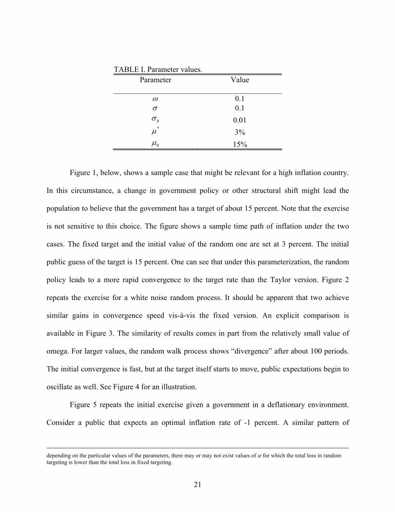
TABLE I. Parameter values. Parameter Value
ω 0.1 σ 0.1
0σ 0.01 *µ 3% 0µ 15%
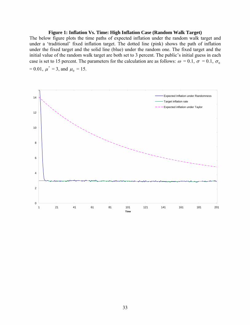
Figure 1, below, shows a sample case that might be relevant for a high inflation country.
In this circumstance, a change in government policy or other structural shift might lead the
population to believe that the government has a target of about 15 percent. Note that the exercise
is not sensitive to this choice. The figure shows a sample time path of inflation under the two
cases. The fixed target and the initial value of the random one are set at 3 percent. The initial
public guess of the target is 15 percent. One can see that under this parameterization, the random
policy leads to a more rapid convergence to the target rate than the Taylor version. Figure 2
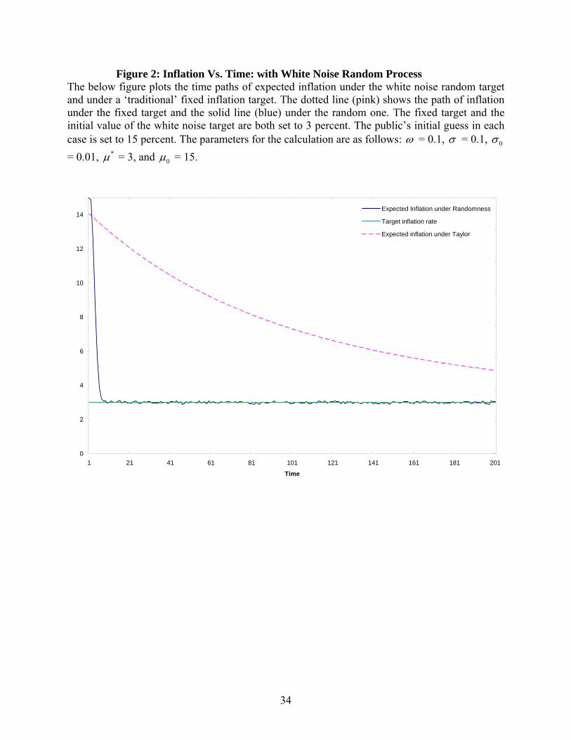
repeats the exercise for a white noise random process. It should be apparent that two achieve
similar gains in convergence speed vis-à-vis the fixed version. An explicit comparison is
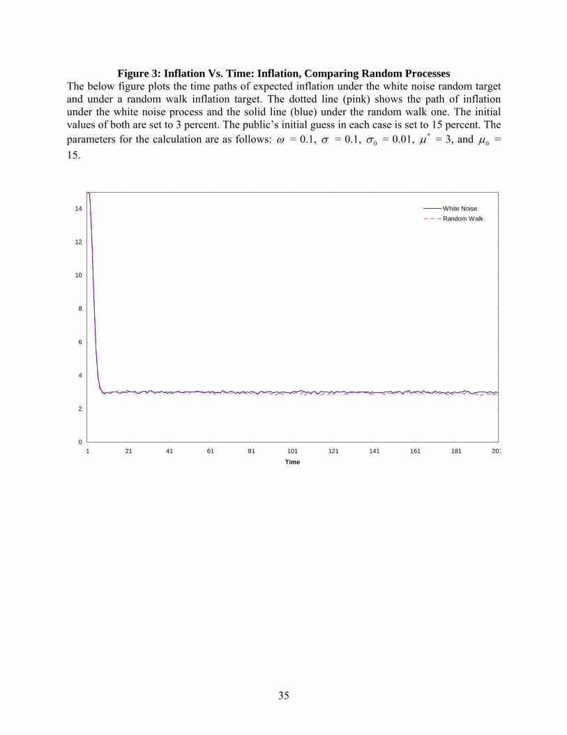
available in Figure 3. The similarity of results comes in part from the relatively small value of
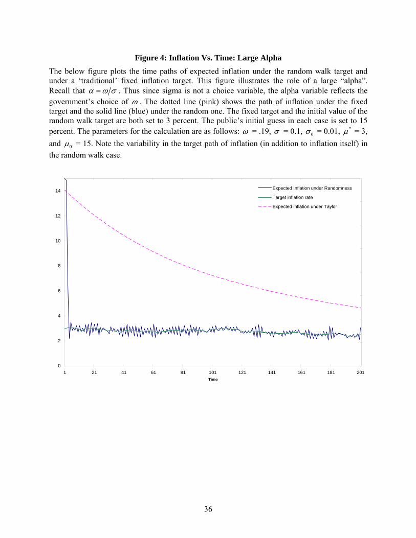
omega. For larger values, the random walk process shows “divergence” after about 100 periods.
The initial convergence is fast, but at the target itself starts to move, public expectations begin to
oscillate as well. See Figure 4 for an illustration.
Figure 5 repeats the initial exercise given a government in a deflationary environment.
Consider a public that expects an optimal inflation rate of -1 percent. A similar pattern of
depending on the particular values of the parameters, there may or may not exist values of α for which the total loss in random targeting is lower than the total loss in fixed targeting.
22
convergence can be seen. We can also consider the squared error and mean squared error for
these cases. Figures 6 and 7 show the squared error and mean squared error respectively for the
high inflation case (comparing the random walk and the fixed versions). Figures 8 and 9 show
the same for the deflationary case.
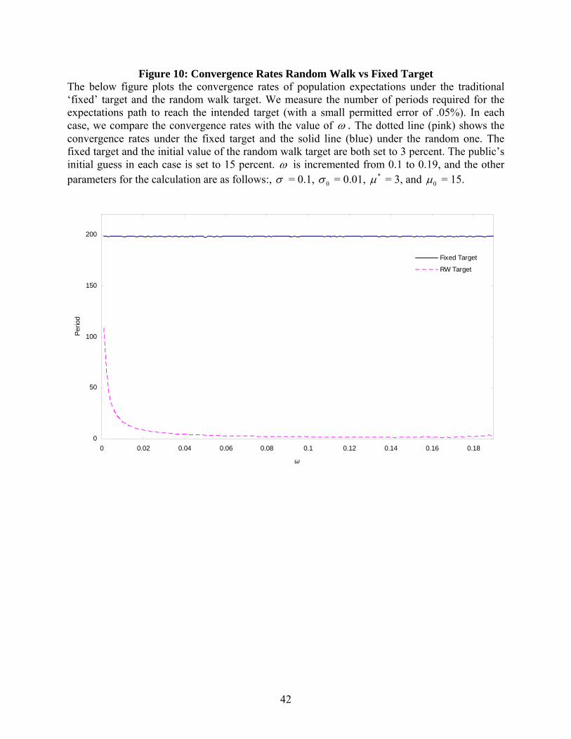
Further exploration reveals a bit more about the properties of this system. The discussion
above suggested that the presence of noise meant that implementation errors were not punished
in the same way as in a fixed system. This allows the populations expectations to converge at a
faster rate. We look at the convergence rate in a number of cases to explore the role of ω in
determining the speed of expectations adjustment. Figure 10 compares the rate of convergence
for the fixed target and the random walk target against the size of ω . Our metric for convergence
is the number of periods to reach the target rate (with some small tolerance). One should be able
to see that the rate of convergence for the random case, and thus its degree of advantage over the
fixed case, is increasing (the number of periods to reach the target is falling) in the ω (and thus
in α ). Figure 11 shows the same set of rates comparing the fixed target to the random process
generated by white noise. Again, the convergence is increasing in ω . Figure 12 compares only
the random walk and white noise processes.
VI. Conclusions
Under rational expectations theory, central banks automatically achieve rapid
convergence of public inflation beliefs to the actual rate of inflation. In many cases, this is not
plausible monetary policy, given credibility constraints. If the public is ignorant of the
parameters of the government’s optimization problem, then the announcement of a new target
will not be automatically credible. This may be particularly true in developing countries where,
because of political instability, the central banks and/or government may minimize a private loss

23
function that does not reflect the societal optimization. We find that in such situations, a
government can achieve faster expectations convergence to an economy’s optimal inflation rate
through the use of a randomized inflation target.
24
References:
Arnold, L., 1974, Stochastic Differential Equations: Theory and Applications (John Wiley and
Sons, New York).
Ball, L., 1994, Credible Disinflation with Staggered Price Setting, The American Economic
Review 84, 282-289.
Ball, L., 1999, Policy Rules for Open Economies,” in Taylor, J., Monetary Policy Rules,
(Chicago University Press, Chicago).
Barro, R. and D. Gordon, 1983, A Positive Theory of Monetary Policy in a Natural Rate Model,
The Journal of Political Economy 91, 589-610.
Bernanke, B., T. Laubach, F. Mishkin, and A. Posen, 1999, Inflation Targeting: Lessons from the
International Experience, (Princeton University Press, Princeton).
Calvo, G., 1983, Staggered Prices in a Utility-Maximizing Framework, Journal of Monetary
Economics 12, 393-98.
Fleming, W., and R. Rishel, 1975, Deterministic and Stochastic Optimal Control. (Springer-
Verlag, New York).
Fischer, S., 1996, Why are Central Banks Pursuing Long-Run Price Stability? in Federal Reserve
Bank of Kansas City, Achieving Price Stability (Federal Reserve Bank of Kansas City,
Kansas City).
King, M., 1996, How Should Central Banks Reduce Inflation? in Federal Reserve Bank of
Kansas City, Achieving Price Stability (Federal Reserve Bank of Kansas City, Kansas
City).
25
Krugman, P., 1998, It’s Baaack, Japan’s Slump and the Return of the Liquidity Trap, Brookings
Papers on Economic Activity.
Kydland, F., and E. Prescott., Rules Rather than Discretion: The Inconsistency of Optimal Plans,
The Journal of Political Economy 85, 473-492.
Sachs, J., Ed., 1990, Developing Country Debt and Economic Performance: Country Studies—
Argentina, Bolivia, Brazil, Mexico. (University of Chicago Press, Chicago).
Sargent, T., 1994, The Ends of Four Big Inflations, in: M. Parkin, ed., The Theory of Inflation,
(Aldershot: UK) 433-89.
Svensson, L., 1996, Commentary: How Should Monetary Policy Respond to Shocks while
Maintaining Long-Run Price Stability? – Conceptual Issues, in Federal Reserve Bank of
Kansas City, Achieving Price Stability (Federal Reserve Bank of Kansas City, Kansas
City).
Svensson, L., 1997, Inflation Forecast Targeting: Implementing and Monitoring Inflation
Targets,” European Economic Review 41, 1111-1146.
Svensson, L., 1999a, Inflation Targeting as a Monetary Policy Rule, Journal of Monetary
Economics 43, 607-654.
Svensson, L., 1999b, Price-Level Targeting Versus Inflation Targeting: A Free Lunch?, Journal
of Money, Credit and Banking 31(3), 277-295.
Taylor, J., 1975, Monetary Policy during a Transition to Rational Expectations, The Journal of
Political Economy 83, 1009-1022.
Taylor, J., 1996, How Should Monetary Policy Respond to Shocks while Maintaining Long-Run
Price Stability? in Federal Reserve Bank of Kansas City, Achieving Price Stability
(Federal Reserve Bank of Kansas City, Kansas City).
26
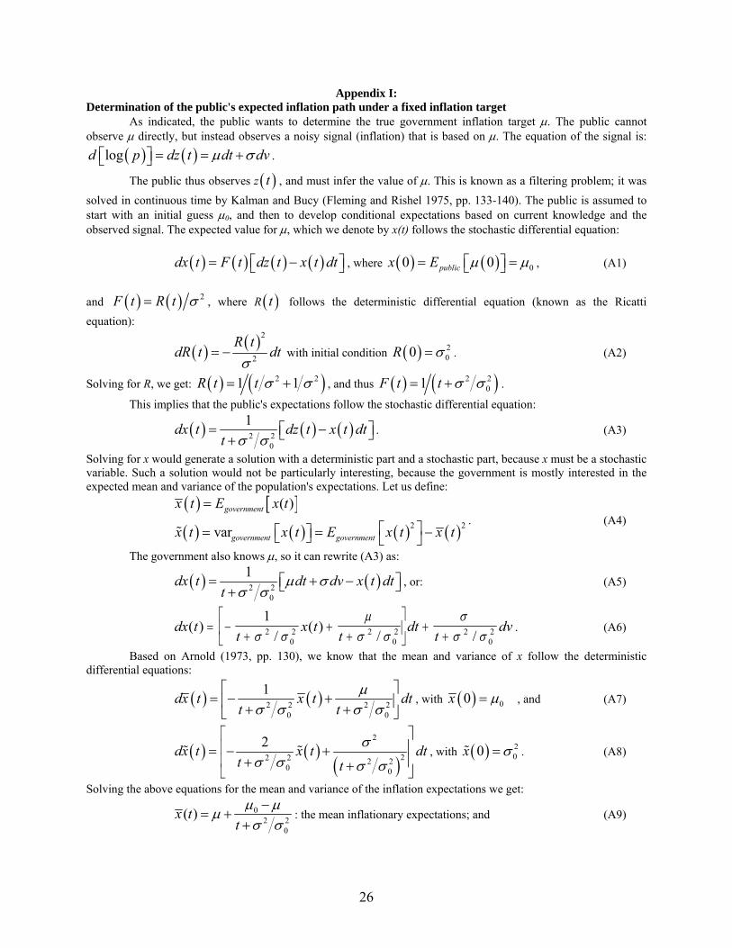
Appendix I: Determination of the public's expected inflation path under a fixed inflation target
As indicated, the public wants to determine the true government inflation target µ. The public cannot observe µ directly, but instead observes a noisy signal (inflation) that is based on µ. The equation of the signal is:
( ) ( )logd p dz t dt dvµ σ= = +⎡ ⎤⎣ ⎦ .
The public thus observes z ( )t , and must infer the value of µ. This is known as a filtering problem; it was solved in continuous time by Kalman and Bucy (Fleming and Rishel 1975, pp. 133-140). The public is assumed to start with an initial guess µ0, and then to develop conditional expectations based on current knowledge and the observed signal. The expected value for µ, which we denote by x(t) follows the stochastic differential equation: ( ) ( ) ( ) ( )dx t F t dz t x t dt= −⎡ ⎤⎣ ⎦ , where ( ) ( ) 00 0publicx E µ µ= =⎡ ⎤⎣ ⎦ , (A1)
and ( ) ( ) 2F t R t σ= , where R ( )t follows the deterministic differential equation (known as the Ricatti equation):
( ) ( )2
2
R tdR t dt
σ= − with initial condition ( ) 2
00R σ= . (A2)
Solving for R, we get: ( ) ( )2 21 1R t t σ σ= + , and thus ( ) ( )2 201F t t σ σ= + .
This implies that the public's expectations follow the stochastic differential equation:
( ) ( ) ( )2 20
1dx t dz t x t dtt σ σ
= −⎡ ⎤⎣ ⎦+. (A3)
Solving for x would generate a solution with a deterministic part and a stochastic part, because x must be a stochastic variable. Such a solution would not be particularly interesting, because the government is mostly interested in the expected mean and variance of the population's expectations. Let us define:
( ) [ ]( ) ( ) ( ) ( )2 2
( )
var
government
government government
x t E x t
x t x t E x t x t
=
⎡ ⎤= = −⎡ ⎤⎣ ⎦ ⎣ ⎦. (A4)
The government also knows µ, so it can rewrite (A3) as:
( ) ( )2 20
1dx t dt dv x t dtt
µ σσ σ
= + −⎡ ⎤⎣ ⎦+, or: (A5)
dx tt
x tt
dtt
dv( )/
( )/ /
= −+
++
⎡
⎣⎢
⎤
⎦⎥ +
+12
02 2
02 2
02σ σ
µσ σ
σσ σ
. (A6)
Based on Arnold (1973, pp. 130), we know that the mean and variance of x follow the deterministic differential equations:
( ) ( )2 2 2 20 0
1dx t x t dtt t
µσ σ σ σ
⎡ ⎤= − +⎢ ⎥+ +⎣ ⎦
, with ( ) 00x µ= , and (A7)
( ) ( )( )
2
22 2 2 20 0
2dx t x t dtt t
σσ σ σ σ
⎡ ⎤⎢ ⎥= − +⎢ ⎥+ +⎣ ⎦
, with ( ) 200x σ= . (A8)
Solving the above equations for the mean and variance of the inflation expectations we get:
02 2
0
( )x ttµ µµσ σ−
= ++
: the mean inflationary expectations; and (A9)
27
( )2
2 20
x tt
σσ σ
=+
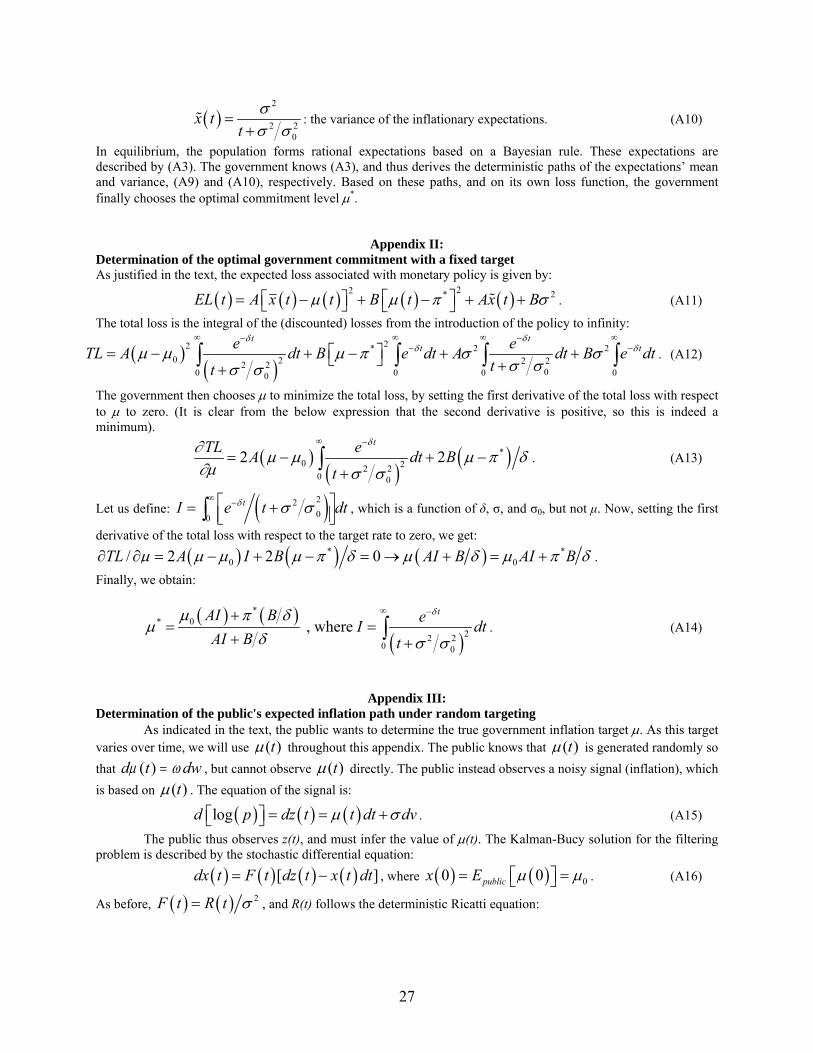
: the variance of the inflationary expectations. (A10)
In equilibrium, the population forms rational expectations based on a Bayesian rule. These expectations are described by (A3). The government knows (A3), and thus derives the deterministic paths of the expectations’ mean and variance, (A9) and (A10), respectively. Based on these paths, and on its own loss function, the government finally chooses the optimal commitment level µ*.
Appendix II: Determination of the optimal government commitment with a fixed target As justified in the text, the expected loss associated with monetary policy is given by:
( ) ( ) ( ) ( ) ( )22 * 2EL t A x t t B t Ax t Bµ µ π σ⎡ ⎤⎡ ⎤= − + − + +⎣ ⎦ ⎣ ⎦ . (A11)
The total loss is the integral of the (discounted) losses from the introduction of the policy to infinity:
( )( )
22 * 2 20 2 2 22 2
00 0 0 00
t tt te eTL A dt B e dt A dt B e dt
tt
δ δδ δµ µ µ π σ σ
σ σσ σ
∞ ∞ ∞ ∞− −− −⎡ ⎤= − + − + +⎣ ⎦ ++
∫ ∫ ∫ ∫ . (A12)
The government then chooses µ to minimize the total loss, by setting the first derivative of the total loss with respect to µ to zero. (It is clear from the below expression that the second derivative is positive, so this is indeed a minimum).
( )( )
( )*0 22 2
0 0
2 2tTL eA dt B
t
δ∂ µ µ µ π δ∂µ σ σ
∞ −
= − + −+
∫ . (A13)
Let us define: ( )2200
tI e t dtδ σ σ∞ −⎡ ⎤= +⎢ ⎥⎣ ⎦∫ , which is a function of δ, σ, and σ0, but not µ. Now, setting the first
derivative of the total loss with respect to the target rate to zero, we get:
( ) ( ) ( )* *0 0/ 2 2 0TL A I B AI B AI Bµ µ µ µ π δ µ δ µ π δ∂ ∂ = − + − = → + = + .
Finally, we obtain:
( ) ( )
( )*
0*22 2
0 0
, where tAI B eI dt
AI B t
δµ π δµ
δ σ σ
∞ −+= =
+ +∫ . (A14)
Appendix III: Determination of the public's expected inflation path under random targeting
As indicated in the text, the public wants to determine the true government inflation target µ. As this target varies over time, we will use ( )tµ throughout this appendix. The public knows that ( )tµ is generated randomly so that d t dwµ ω( ) = , but cannot observe ( )tµ directly. The public instead observes a noisy signal (inflation), which is based on ( )tµ . The equation of the signal is:
( ) ( ) ( )logd p dz t t dt dvµ σ= = +⎡ ⎤⎣ ⎦ . (A15)
The public thus observes z(t), and must infer the value of µ(t). The Kalman-Bucy solution for the filtering problem is described by the stochastic differential equation: ( ) ( ) ( ) ( )[ ]dx t F t dz t x t dt= − , where ( ) ( ) 00 0publicx E µ µ= =⎡ ⎤⎣ ⎦ . (A16)
As before, ( ) ( ) 2F t R t σ= , and R(t) follows the deterministic Ricatti equation:
28
( ) ( )22
2
R tdR t dtω
σ
⎡ ⎤= − +⎢ ⎥⎢ ⎥⎣ ⎦
with initial condition ( ) 200R σ= . (A17)
Solving for R, we get:
( )220
2 20
1 , where / and 1
t
t
CeR t CCe
α
α
ωσ σσω α ω σωσ σ
+−= = =
+ −, (A18)
and thus:
F tCeCe
Ct
t( ) /=−+
= =+−
α α ω σωσ σωσ σ
α
α
2
202
02
11
, where and . (A19)
This implies that the public's expectations follow the stochastic differential equation:
( ) ( ) ( )2
2
1[ ]1
t
t
Cedx t dz t x t dtCe
α
αα −= −
+. (A20)
Let us define as before:
( ) ( )
( ) ( ) ( ) ( )2var
government
government government
x t E x t
x t x t E x t x t
= ⎡ ⎤⎣ ⎦⎡ ⎤= = −⎡ ⎤⎣ ⎦ ⎣ ⎦
. (A21)
Rewriting (A20) based on (A15) and the definition of ( )tµ , we obtain:
( ) ( ) ( )2
2
11
t
t
Cedx t t dt dv x t dtCe
α
αα µ σ−⎡ ⎤= + −⎣ ⎦+
, or: (A22)
( ) ( )2 2 2
2 2 2
1 1 11 1 1
t t t
t t t
Ce Ce Cedx t x t dt dvCe Ce Ce
α α α
α α αα µ σα⎡ ⎤− − −
= − + +⎢ ⎥+ + +⎣ ⎦ (A23)
Based on Arnold (1973) the mean and variance of x follow the deterministic differential equations:
( ) ( ) ( )2 2
2 2
1 11 1
t t
t t
Ce Cedx t x t t dtCe Ce
α α
α αα µ α⎡ ⎤− −
= − +⎢ ⎥+ +⎣ ⎦, with x( )0 0= µ , and (A24)
( ) ( ) ( )22 2
2 2 22 2
1 121 1
t t
t t
Ce Cedx t x t dtCe Ce
α α
α αα α σ ω⎡ ⎤⎛ ⎞− −
= − + +⎢ ⎥⎜ ⎟+ +⎢ ⎥⎝ ⎠⎣ ⎦, with ( ) 2
00x σ= . (A25)
Solving the above equations for the mean and variance of the inflation expectations we get:
( ) ( ) ( ) ( ) ( )20
0 2
2 , where and t tx t t te eα α
σα ωµ µ µ α βα β α β σ σ−⎡ ⎤= + − = =⎣ ⎦ + + −
, and (A26)
( ) ( ) ( ) ( )( )( ) ( )( )( ) ( )
22 2 2 2 2 2 22
2
2 1 1 1 2 11
2
t
t t
t ex t
e e
α
α α
α α β α α α β α α α α βα αα β α β
−
−
− − + − + − + −= + +
⎡ ⎤+ + −⎣ ⎦. (A27)
Appendix IV: Determination of the optimal government commitment with a random target
As before, the expected loss at each time t is given by:
( ) ( ) ( ) ( ) ( ) ( )22 * 2 2EL t A x t t B t Ax t Bµ µ π σ ω⎡ ⎤⎡ ⎤= − + − + + +⎣ ⎦ ⎣ ⎦ . (A28)
It follows that the total loss is

29
( )( )( ) ( )
( ) ( ) ( )
2 22
0 22 20 0 0
2* 2 2
0 0 0
4 t
t t
t t t
eTL A t dte e
B t e dt A e x t dt B e dt
δ
α α
δ δ δ
σ ωµ µσω σ σω σ
µ π σ ω
∞ −
−
∞ ∞ ∞− − −
= − +⎡ ⎤+ + −⎣ ⎦
⎡ ⎤− + + +⎣ ⎦
∫
∫ ∫ ∫. (A29)
To optimize governmental policy, let us first determine the best monetary target under the temporary assumption that ω is constant (that is, not a choice variable). This is achieved by setting the derivative of the total loss function with respect to the target rate to zero:
( ) ( )( ) ( )
( )2 2
*0 22 2
0 0 0
42 2
t
t t
eTL A t dt B te e
δ
α α
σ ω∂ µ µ µ π δ∂µ σω σ σω σ
−∞
−⎡ ⎤⎡ ⎤= − + −⎣ ⎦ ⎣ ⎦⎡ ⎤+ + −⎣ ⎦
∫ .
(A30)
Let us define: ( ) ( ) ( ) 22 2 2 20 00
( ) 4 t t tJ e e e dtδ α αω σ ω σω σ σω σ∞ −⎡ ⎤ ⎡ ⎤≡ + + −⎣ ⎦ ⎣ ⎦∫ , which again does
not depend on ( )tµ . Now, setting the first derivative of the total loss with respect to the target rate to zero, we get:
( ) ( ) ( )( )( ) ( ) ( )( )
22 2 2 20 00
* *0 0
/ ( ) 4
2 2 0
t t tTL J t e e e dt
A t J B t t AJ B AJ B
δ α αµ σ ω σω σ σω σ
µ µ µ π δ µ δ µ π δ
∞ −⎡ ⎤ ⎡ ⎤∂ ∂ ≡ + + −⎣ ⎦ ⎣ ⎦⎡ ⎤= − + − = → + = +⎣ ⎦
∫ .
Finally, we obtain
( ) ( ) ( )( )
*0* AJ B
AJ Bµ ω π δ
µ ωω δ
+⎡ ⎤⎣ ⎦=+
,where (A31)
( ) ( )
220
2 20
4 , and .t
t t
eJ dte e
δ
α α
σα ωα βσ σα β α β
∞ −
−≡ = =
⎡ ⎤+ + −⎣ ⎦∫
In equilibrium, the government should choose a target inflation rate described by (A31) for any particular (predetermined) level of randomization ω. Subsequently, the government should choose the particular level of randomization ω* that minimizes the total loss function (A29). Due to the complexities of the equations involved, a closed solution for ω* is not available.
Appendix V Comparison of expectations convergence speed under fixed and random targets
We attempt to show that the (expected) convergence of the expectations towards the true target rate is faster under random targeting (A26) than under fixed targeting (A9). Let f t e tt( ) ,= ∈ ℜα be an exponential function, with α = ω/σ as above. Since f is convex, we have from Jensen's inequality:
( ) ( ) ( ) ( )1 2 1 2
1 2
1 1 ,
, ,
s f t s f t f s t s t
t t s
⋅ + − ⋅ ≥ ⋅ + − ⋅⎡ ⎤⎣ ⎦∀ ∈ℜ
(A32)
In particular, let us set: t1 = t; t2 = - t , and σωσϖω 2/)( 20+=s . From the above inequality (A32), we get:
σω σ
σωσω σ
σωα α α
σσω
σσ
++
−≥ =−0
202
2 2
02
02
2e e e et t t t. (A33)
But for any value q, we know that e qq ≥ +1 . In particular:
202
2 2 20 02 2 2
0
1t
e t tσσ σ σ σ
σ σ σ⎛ ⎞
≥ + = +⎜ ⎟⎝ ⎠
. (A34)
30
Based on the fact that σ corresponds to the maximum inflation generation precision, it follows that:
σ σσσ
≤ ≥0 1, . and so we also have: 02
2 (A35)
Combining (A33), (A34) and (A35), we get:
σω σ
σωσω σ
σωσσ
α α++
−≥ +−0
202 2
022 2
e e tt t . (A36)
Inverting, we obtain:
σω σ
σωσω σ
σωσσ
α α++
−⎛⎝⎜
⎞⎠⎟ ≤ +
⎛⎝⎜
⎞⎠⎟−
− −
02
02 1 2
02
1
2 2e e tt t . (A37)
Multiplying by 0 ( )tµ µ− we obtain:
( )( )
( ) ( )( ) ( )0 0
022 20 0
20
2, iff .
t t
t tt
e e tα α
σω µ µ µ µµ µ
σσω σ σω σσ
−
− −≤ <
+ + − + And, (A38a)
( )
( ) ( )( ) ( )0 0
022 20 0
20
2, iff .
t t
t tt
e e tα α
σω µ µ µ µµ µ
σσω σ σω σσ
−
⎡ ⎤− −⎣ ⎦ ≥ >+ + − +
(A38b)
The above equations, together with the equations (A26) and (A9), show that the convergence of x towards µ is always faster under random targeting than under fixed rate targeting. Moreover, if we compare (A14) and (A31), with (A37), we find that the weighting factor I that appears in the fixed rate optimization problem is always higher than the factor J that appears in the random rate optimization. Indeed, squaring (A37) and using the definitions of I and J, we obtain that ( ) , 0.I J ω ω≥ ∀ > In particular, this implies that the optimal target under
randomization will be always closer to the socially desired level π* than will the optimal rate under a fixed target policy.
Appendix VI Comparison of total losses under fixed and random targets
We have shown that optimality in the fixed and randomized targeting cases requires the government to choose µF
* and α*, µR* (α*) respectively. These choices generate respective values of the loss function of
( )* *F FTL TL µ= and ( )* *F RTL TL µ α= ⎡ ⎤⎣ ⎦ . Below, we establish a sufficient (but not necessary) condition
for *RTL to be lower than *FTL . For simplicity, calculations below are carried out using the symbols
σωα /= and 220 /σσβ = .
Lemma 1: Under random targeting, ( ) ( ) ( )22
0lim 1 1 , 0x t t t tα
σ β β→
⎡ ⎤= + + ∀ >⎣ ⎦ .
Proof of Lemma 1: Starting with the formula for ( )x t in (A27), we apply the L’Hospital rule twice, since
α is the only variable factor. The fact that the resulting limit exists and is finite proves the lemma (for clarity of exposition, actual calculations are skipped here). Lemma 2: Let µF
* be the optimal inflation target chosen under fixed targeting, and ( )* *F FTL TL µ= the total
loss associated with it. Also, for a given α > 0, let µ R* (α) be the optimal inflation target chosen under
random targeting, and ( ) ( )* *R RTL TLα µ α= ⎡ ⎤⎣ ⎦ . Then, the following relation
holds: ( )* *
0lim R R FTL TLα
µ α→
⎡ ⎤ ≤⎣ ⎦ , with equality iff .1=β
31
Proof of Lemma 2: We know that
( )( )*F R RTL TL µ α− =
( )( )
22 * 2 20 2 2 22 2
00 0 0 00//
t tt te eA dt B e dt A dt B e dt
tt
δ δδ δµ µ µ π σ σ
σ σσ σ
∞ ∞ ∞ ∞− −− −⎡ ⎤− + − + + −⎣ ⎦ ++
∫ ∫ ∫ ∫
( )( )( ) ( )
( ) ( ) ( )2 2 22 * 2 2
0 22 20 0 0 00 0
4
[
tt t t
t t
eA t dt B t e dt A e x t dt B e dte e
δδ δ δ
α α
σ ωµ µ µ π σ ωσω σ σω σ
∞ ∞ ∞ ∞−− − −
−⎡ ⎤− − − − − − +⎣ ⎦⎡ ⎤+ + −⎣ ⎦
∫ ∫ ∫ ∫
. (A39)
In the above equality, let us take 0α → , which also implies 0ω → . First of all, from the derivation in
Appendix V (or simply applying the l’Hospital rule twice) we have that:
( )( ) ( )
( )( ) ( )
2 2 2 22 2
0 02 20 02 2 2 20 00 0 0 0
4 4lim limt t
t t t t
e eA dt A dte e e e
δ δ
α αα α α α
σ ω σ ωµ µ µ µσω σ σω σ σω σ σω σ
∞ ∞− −
→ →− −
⎧ ⎫⎪ ⎪− = − =⎨ ⎬
⎡ ⎤ ⎡ ⎤+ + − + + −⎪ ⎪⎣ ⎦ ⎣ ⎦⎩ ⎭∫ ∫
( )( )
20 22 2
0 0
./
teA dtt
δ
µ µσ σ
∞ −
= −+
∫ (A39a)
Second, it is trivial to see that:
( ) ( )2 2 2 2 2
0 00 0 0
lim lim .t t tB e dt B e dt B e dtδ δ δ
α ασ ω σ ω σ
∞ ∞ ∞− − −
→ →+ = + =∫ ∫ ∫ (A40)
Using the above (A39) and (A40) results, we obtain:
( )*
0limF R RTL TLα
µ α→
⎡ ⎤− =⎣ ⎦ ( )22 2 0
00 0
lim/
tteA dt A e x t dt
t
δδ
ασ
σ σ
∞ ∞−−
→⎡ ⎤− ⎣ ⎦+∫ ∫ . (A41)
Based on Lemma 1, we can simplify further:
( )*
0limF R RTL TLα
µ α→
⎡ ⎤− =⎣ ⎦( )
( )2
20
111/ 1
t tA e dt
t tδ β
σβ β
∞−
⎡ ⎤+−⎢ ⎥
+ +⎢ ⎥⎣ ⎦∫ =
( )( )
22
0
11 1
t tA e dt
t tδ ββσ
β β
∞−
⎡ ⎤+− =⎢ ⎥
+ +⎢ ⎥⎣ ⎦∫
( )
22
20 1
t t tA e dtt
δ β β β βσβ
∞−
⎡ ⎤+ − −= =⎢ ⎥
+⎢ ⎥⎣ ⎦∫
( )( )
22
0
11
t tA e dt
tδ β β
σβ
∞− −
+∫ . (A42)
Since by construction 1β ≥ , it follows that ( ) ( )22
01 / 1 0tA e t t dtδσ β β β
∞ − − + ≥⎡ ⎤⎣ ⎦∫ , with equality iff
1β = . Combining this with (A42), we reach the desired conclusion, namely, that: ( )* *
0lim R R FTL TLα
µ α→
⎡ ⎤ ≤⎣ ⎦ , with equality iff .1=β (A43)
Lemma 3: With the same notation as above, ( )*lim R RTLα
µ α→∞
⎡ ⎤ = ∞⎣ ⎦ .
Proof of Lemma 3: The result is derived trivially by passing α to infinity in (A28) and noticing that the first three terms are all positive and that the last one is infinite. Theorem 1: If 0σ σ> , that is, if 1β > , then ∃ > =ω α ω σ0 (and thus / ) , such that
( ) ( )* 0,R R FTL TLµ α α α⎡ ⎤ < ∀ ∈⎣ ⎦ .
32
Proof of Theorem 1: Since β > 1, we know from Lemma 2 that ( )* *
0lim R R FTL TLα
µ α→
⎡ ⎤ <⎣ ⎦ , This implies
that there exists a neighborhood of zero, say, N = (0, 2ε) with ε > 0, such that: ( ) ( )* * , 0, 2 .R R FTL TL Nµ α ε ε⎡ ⎤ < ∀ ∈ =⎣ ⎦ (A44)
In particular, it follows that: ( )* *0 .R R FTL TLε µ ε⎡ ⎤∃ > ∴ <⎣ ⎦ (A44a)
From Lemma 3, we know that ( )*lim .R RTLα
µ α→∞
⎡ ⎤ = ∞⎣ ⎦ This implies that there exists a neighborhood of infinity,
say N’ = (δ/2,∝) with δ > ε > 0, such that: ( ) ( )* * , / 2, .R R FTL TL Nµ α ε δ′⎡ ⎤ < ∀ ∈ = ∞⎣ ⎦ (A45)
In particular, it follows that: ( )* *
R R FTL TLδ ε µ δ⎡ ⎤∃ > ∴ >⎣ ⎦ (A45a)
The expressions (A44a) and (A45a) show that the function ( )*R RTL µ⎡ ⎤⋅⎣ ⎦ takes values both below and above TL*F.
But ( )*R RTL µ α⎡ ⎤⎣ ⎦ is a continuous function of α, and thus (A44a) and (A45a) guarantee that:
( ) ( )*ˆ ˆ, .R R FTL TLα ε δ µ α⎡ ⎤∃ ∈ ∴ =⎣ ⎦ (A46)
Let us now define the set A as follows: ( )* *{ 0 | R R FA x TL x TLµ⎡ ⎤= > =⎣ ⎦ . Expression (A46) guarantees
that the set A is non-empty. Let α = infx
A . We can easily see that α > 0 . Indeed, if this were not the case, there
would exist points x arbitrarily close to zero such that ( )* .R R FTL x TLµ⎡ ⎤ =⎣ ⎦ But this contradicts (A45), which says
that there exists an entire neighborhood of zero with points for which the relation above is not true. We contend now
that the α > 0 as defined above has the desired property: ( ) ( )* * 0,R R FTL TLµ α ε α⎡ ⎤ < ∀ ∈⎣ ⎦ . Indeed, suppose
by contradiction that this were not the case, that is, ( ) ( )*0, R R FTL TLθ α µ θ⎡ ⎤∃ ∈ ∴ >⎣ ⎦ (A47)
From (A45) we know that ( )*R RTL µ⎡ ⎤⋅⎣ ⎦ must take a value lower than TL*F in ( )0,α . If (A47) were true, then the
function would also take a value greater than TL*F. By reason of continuity of the function ( )*R RTL µ⎡ ⎤⋅⎣ ⎦ , we
conclude that ( ) ( )* *0, R R FTL TLγ α µ γ⎡ ⎤∃ ∈ ∴ =⎣ ⎦ . It follows that γ ∈ A and thus, by construction,
γ α≥ = inf .x
A But this contradicts the fact that by construction ( )0,γ α∈ . It follows that (A47) cannot be true,
and thus we conclude that: ( ) ( )* *0 0,R R FTL TLα µ α α⎡ ⎤∃ > ∴ < ∀∈⎣ ⎦ (A48).
33
Figure 1: Inflation Vs. Time: High Inflation Case (Random Walk Target) The below figure plots the time paths of expected inflation under the random walk target and under a ‘traditional’ fixed inflation target. The dotted line (pink) shows the path of inflation under the fixed target and the solid line (blue) under the random one. The fixed target and the initial value of the random walk target are both set to 3 percent. The public’s initial guess in each case is set to 15 percent. The parameters for the calculation are as follows: ω = 0.1, σ = 0.1, 0σ = 0.01, *µ = 3, and 0µ = 15.
0
2
4
6
8
10
12
14
1 21 41 61 81 101 121 141 161 181 201Time
Expected Inflation under Randomness
Target inflation rate
Expected inflation under Taylor
34
Figure 2: Inflation Vs. Time: with White Noise Random Process The below figure plots the time paths of expected inflation under the white noise random target and under a ‘traditional’ fixed inflation target. The dotted line (pink) shows the path of inflation under the fixed target and the solid line (blue) under the random one. The fixed target and the initial value of the white noise target are both set to 3 percent. The public’s initial guess in each case is set to 15 percent. The parameters for the calculation are as follows: ω = 0.1, σ = 0.1, 0σ = 0.01, *µ = 3, and 0µ = 15.
0
2
4
6
8
10
12
14
1 21 41 61 81 101 121 141 161 181 201
Time
Expected Inflation under Randomness
Target inflation rate
Expected inflation under Taylor
35
Figure 3: Inflation Vs. Time: Inflation, Comparing Random Processes The below figure plots the time paths of expected inflation under the white noise random target and under a random walk inflation target. The dotted line (pink) shows the path of inflation under the white noise process and the solid line (blue) under the random walk one. The initial values of both are set to 3 percent. The public’s initial guess in each case is set to 15 percent. The parameters for the calculation are as follows: ω = 0.1, σ = 0.1, 0σ = 0.01, *µ = 3, and 0µ = 15.
0
2
4
6
8
10
12
14
1 21 41 61 81 101 121 141 161 181 201
Time
White NoiseRandom Walk
36
Figure 4: Inflation Vs. Time: Large Alpha
The below figure plots the time paths of expected inflation under the random walk target and under a ‘traditional’ fixed inflation target. This figure illustrates the role of a large “alpha”. Recall that α ω σ= . Thus since sigma is not a choice variable, the alpha variable reflects the government’s choice of ω . The dotted line (pink) shows the path of inflation under the fixed target and the solid line (blue) under the random one. The fixed target and the initial value of the random walk target are both set to 3 percent. The public’s initial guess in each case is set to 15 percent. The parameters for the calculation are as follows: ω = .19, σ = 0.1, 0σ = 0.01, *µ = 3, and 0µ = 15. Note the variability in the target path of inflation (in addition to inflation itself) in the random walk case.
0
2
4
6
8
10
12
14
1 21 41 61 81 101 121 141 161 181 201Time
Expected Inflation under Randomness
Target inflation rate
Expected inflation under Taylor

37
Figure 5: Inflation Vs. Time: Deflation Case The below figure plots the time paths of expected inflation under the random walk target and under a ‘traditional’ fixed inflation target. The dotted line (pink) shows the path of inflation under the fixed target and the solid line (blue) under the random one. The fixed target and the initial value of the random walk target are both set to 3 percent. The public’s initial guess in each case is set to minus one percent. The parameters for the calculation are as follows: ω = 0.1, σ = 0.1, 0σ = 0.01, *µ = 3, and 0µ = -1.
-1
-0.5
0
0.5
1
1.5
2
2.5
3
3.5
1 21 41 61 81 101 121 141 161 181 201Time
Expected Inflation under Randomness
Target inflation rate
Expected inflation under Taylor
38
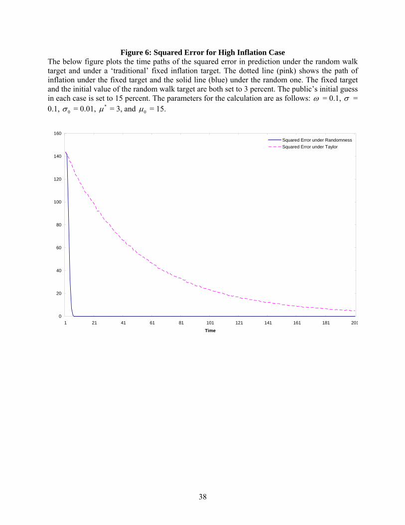
Figure 6: Squared Error for High Inflation Case The below figure plots the time paths of the squared error in prediction under the random walk target and under a ‘traditional’ fixed inflation target. The dotted line (pink) shows the path of inflation under the fixed target and the solid line (blue) under the random one. The fixed target and the initial value of the random walk target are both set to 3 percent. The public’s initial guess in each case is set to 15 percent. The parameters for the calculation are as follows: ω = 0.1, σ = 0.1, 0σ = 0.01, *µ = 3, and 0µ = 15.
0
20
40
60
80
100
120
140
160
1 21 41 61 81 101 121 141 161 181 201
Time
Squared Error under RandomnessSquared Error under Taylor

39
Figure 7: Mean Squared Error for High Inflation Case The below figure plots the paths of the mean squared error, from time zero to present, in prediction under the random walk target and under a ‘traditional’ fixed inflation target. The dotted line (pink) shows the path of inflation under the fixed target and the solid line (blue) under the random one. The fixed target and the initial value of the random walk target are both set to 3 percent. The public’s initial guess in each case is set to 15 percent. The parameters for the calculation are as follows: ω = 0.1, σ = 0.1, 0σ = 0.01, *µ = 3, and 0µ = 15.
0
20
40
60
80
100
120
140
160
1 21 41 61 81 101 121 141 161 181 201
Time
Mean Squared Error under RandomnessMean Squared Error under Taylor
40
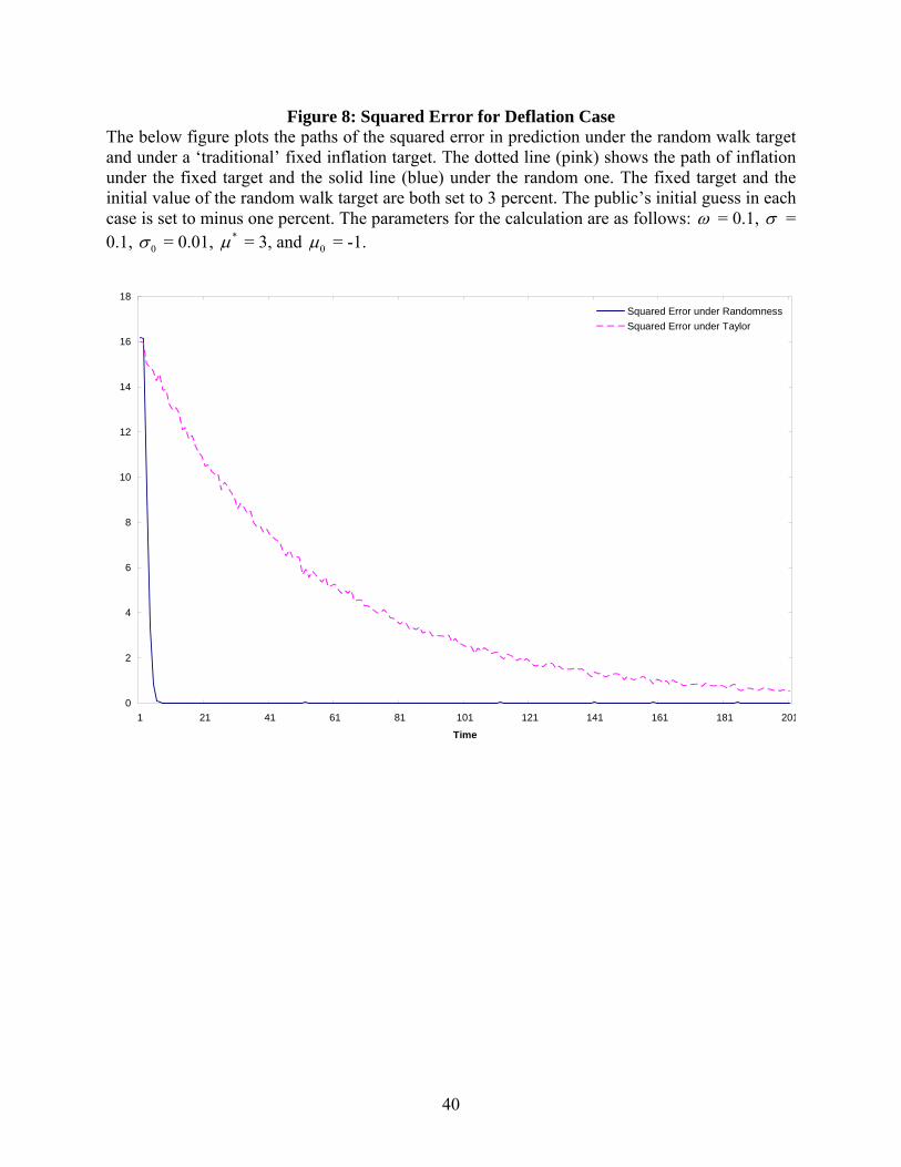
Figure 8: Squared Error for Deflation Case The below figure plots the paths of the squared error in prediction under the random walk target and under a ‘traditional’ fixed inflation target. The dotted line (pink) shows the path of inflation under the fixed target and the solid line (blue) under the random one. The fixed target and the initial value of the random walk target are both set to 3 percent. The public’s initial guess in each case is set to minus one percent. The parameters for the calculation are as follows: ω = 0.1, σ = 0.1, 0σ = 0.01, *µ = 3, and 0µ = -1.
0
2
4
6
8
10
12
14
16
18
1 21 41 61 81 101 121 141 161 181 201
Time
Squared Error under RandomnessSquared Error under Taylor
41
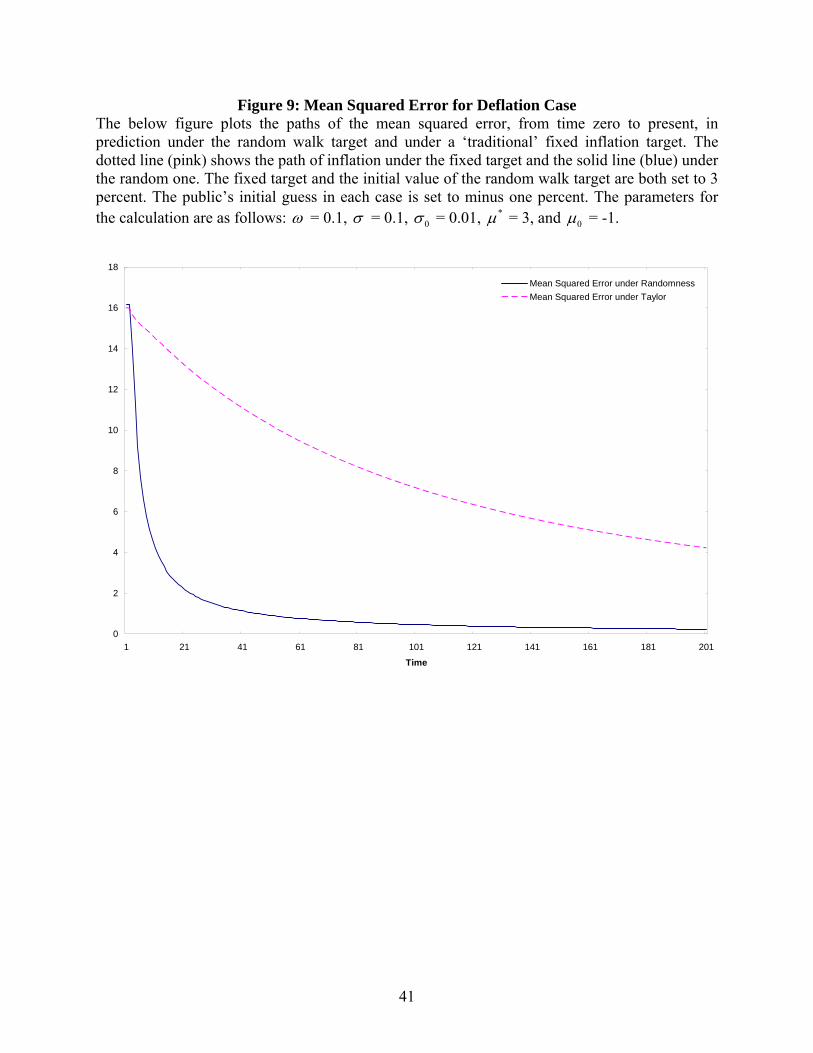
Figure 9: Mean Squared Error for Deflation Case The below figure plots the paths of the mean squared error, from time zero to present, in prediction under the random walk target and under a ‘traditional’ fixed inflation target. The dotted line (pink) shows the path of inflation under the fixed target and the solid line (blue) under the random one. The fixed target and the initial value of the random walk target are both set to 3 percent. The public’s initial guess in each case is set to minus one percent. The parameters for the calculation are as follows: ω = 0.1, σ = 0.1, 0σ = 0.01, *µ = 3, and 0µ = -1.
0
2
4
6
8
10
12
14
16
18
1 21 41 61 81 101 121 141 161 181 201
Time
Mean Squared Error under RandomnessMean Squared Error under Taylor
42
Figure 10: Convergence Rates Random Walk vs Fixed Target The below figure plots the convergence rates of population expectations under the traditional ‘fixed’ target and the random walk target. We measure the number of periods required for the expectations path to reach the intended target (with a small permitted error of .05%). In each case, we compare the convergence rates with the value of ω . The dotted line (pink) shows the convergence rates under the fixed target and the solid line (blue) under the random one. The fixed target and the initial value of the random walk target are both set to 3 percent. The public’s initial guess in each case is set to 15 percent. ω is incremented from 0.1 to 0.19, and the other parameters for the calculation are as follows:, σ = 0.1, 0σ = 0.01, *µ = 3, and 0µ = 15.
0
50
100
150
200
0 0.02 0.04 0.06 0.08 0.1 0.12 0.14 0.16 0.18
ω
Perio
d
Fixed Target
RW Target
43
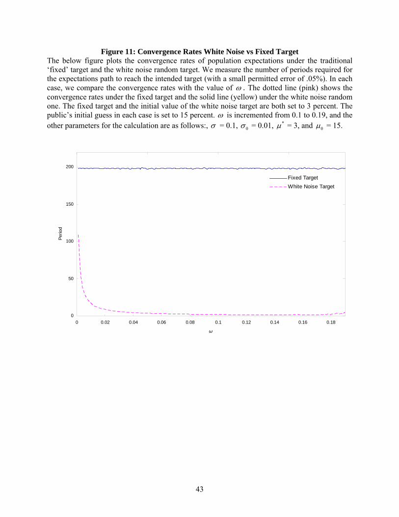
Figure 11: Convergence Rates White Noise vs Fixed Target The below figure plots the convergence rates of population expectations under the traditional ‘fixed’ target and the white noise random target. We measure the number of periods required for the expectations path to reach the intended target (with a small permitted error of .05%). In each case, we compare the convergence rates with the value of ω . The dotted line (pink) shows the convergence rates under the fixed target and the solid line (yellow) under the white noise random one. The fixed target and the initial value of the white noise target are both set to 3 percent. The public’s initial guess in each case is set to 15 percent. ω is incremented from 0.1 to 0.19, and the other parameters for the calculation are as follows:, σ = 0.1, 0σ = 0.01, *µ = 3, and 0µ = 15.
0
50
100
150
200
0 0.02 0.04 0.06 0.08 0.1 0.12 0.14 0.16 0.18
ω
Perio
d
Fixed TargetWhite Noise Target
44
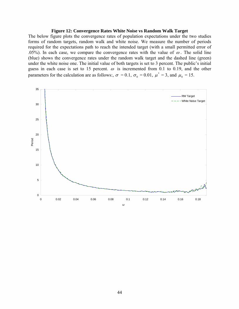
Figure 12: Convergence Rates White Noise vs Random Walk Target The below figure plots the convergence rates of population expectations under the two studies forms of random targets, random walk and white noise. We measure the number of periods required for the expectations path to reach the intended target (with a small permitted error of .05%). In each case, we compare the convergence rates with the value of ω . The solid line (blue) shows the convergence rates under the random walk target and the dashed line (green) under the white noise one. The initial value of both targets is set to 3 percent. The public’s initial guess in each case is set to 15 percent. ω is incremented from 0.1 to 0.19, and the other parameters for the calculation are as follows:, σ = 0.1, 0σ = 0.01, *µ = 3, and 0µ = 15.
0
5
10
15
20
25
30
35
0 0.02 0.04 0.06 0.08 0.1 0.12 0.14 0.16 0.18
ω
Perio
d
RW Target
White Noise Target
Top Related