


Languages
Pages
Legal

1
Improving warehouse responsiveness by job priority management:
A European distribution centre field study
Thai Young Kim1
Econometric Institute Report EI2018-02
Abstract
Warehouses employ order cut-off times to ensure sufficient time for fulfilment. To satisfy
higher consumer expectations, these cut-off times are gradually postponed to improve order
responsiveness. Warehouses therefore have to allocate jobs more efficiently to meet
compressed response times. Priority job management by means of flow-shop models has
been used mainly for manufacturing systems but can also be applied for warehouse job
scheduling to accommodate tighter cut-off times. This study investigates which priority rule
performs best under which circumstances. The performance of each rule is evaluated in terms
of a common cost criterion that integrates the objectives of low earliness, low tardiness, low
labour idleness, and low work-in-process stocks. A real-world case study for a warehouse
distribution centre of an original equipment manufacturer in consumer electronics provides
the input parameters for a simulation study. The simulation outcomes validate several
strategies for improved responsiveness. In particular, the critical ratio rule has the fastest
flow-time and performs best for warehouse scenarios with expensive products and high
labour costs.
Keywords
responsiveness; queuing model; order fulfilment; cut-off operation; flow-shop scheduling
1 The author thanks Rommert Dekker and Christiaan Heij for their assistance in this research project and for their substantial language support.
2
1. Introduction
Intense competition for speedy order fulfilment characterizes current retail markets.
Responsiveness (Barclay et al., 1996) includes the ability to react purposefully within an
appropriate time to external environments for securing competitive advantage. Improving order
fulfilment responsiveness is a major challenge for boosting customer satisfaction (Doerr and Gue,
2013) and many firms, such as Amazon Prime, invest hefty capital to propel responsiveness.
Though responsiveness hones competitiveness, it often leads to resource misallocation (T’kindt,
2011), and improved responsiveness leads for two-thirds of all firms to increased labour cost
(Pearcy and Kerr, 2013). Web retailers show responsiveness by advertising ‘Place an order before
midnight for next-day delivery.’ Customers are nowadays accustomed to such fast demand
satisfaction in on-line markets and expect comparable off-line service. Off-line retailers therefore
attract customers with promises like ‘Buy online now and pick up in store tomorrow’, forcing off-
line retail distributors to improve their responsiveness (Denman, 2017).
The overall speed of order fulfilment in off-line markets depends on processing and
transportation speeds from manufacturers through warehouses and retail shops to end-users. This
paper focuses on speedy order fulfilment in warehouses, in particular original equipment
manufacturing (OEM) warehouses delivering to retailer warehouses. Their order fulfilment
process includes the inbound processes of receiving products and putting them away and the
outbound processes of picking, packing, staging and shipping. As OEM warehouses receive
products from their manufacturer, the inbound process is easily controlled compared to the rather
unpredictable consumer demand leading to fast fluctuations of retailer orders. Another
characteristic of OEM warehouses is that retailers order relatively large quantities of relatively few
products (Bartholdi and Hackman, 2011). This distinguishes such warehouses from those
delivering directly to consumers, where order sizes are small and range over a much wider product
assortment. Whereas picking is usually the crucial stage for the latter type, in OEM warehouses
the packing stage is often the most demanding one. As the receiving retailer warehouses differ in
capacity and lay-out and trucks should be loaded efficiently, re-palletizing is a major task for OEM
warehouses. Because of the large order volumes, the re-palletizing activities of unpacking,
repacking and stacking are relatively labour intensive.

3
Responsiveness of OEM warehouses is measured by their flexibility to dispatch products
ordered by retailers as fast as possible. To mitigate the effect of demand spikes, most OEM
warehouses limit their fulfilment liability by daily order cut-off time agreements with their clients
to ensure sufficient slack for order fulfilment by the earliest dispatch day (Van den Berg, 2007).
To improve responsiveness, these warehouses try to postpone the cut-off time and to handle the
same order volume with less slack. Since orders typically have different fulfilment deadlines,
priority-based job scheduling offers the key for efficient solutions. Just as job scheduling has
notably reduced waste from over-production and waiting times in “just-in-time” manufacturing, it
can also improve responsiveness in warehouse order fulfilment. Job scheduling allocates tasks to
labour resources for chosen goals (T’kindt and Billaut, 2006), and the question of central interest
here is how OEM warehouses should schedule their orders to allow later cut-off times.
Warehouse operations are faced with various uncertainties, including dynamic arrival,
service and departure times (Gong and De Koster, 2011). In particular, unexpected order arrivals
can yield long delays. Because of these uncertainties there is usually no priority rule that is
universally optimal (Lee et al., 1997). This paper presents a general framework for cost-effective
job scheduling using flow-shop priority methods to aid warehouses facing postponed order cut-off
times. This framework integrates the multiple objectives of low earliness, low tardiness, low labour
idleness, and low stocks through processing lanes into a single cost criterion, with weights derived
from the cost structure and performance priorities of the warehouse. A simulation study shows
which scheduling methods perform best under which circumstances. The methods and results
presented here advance extant literature by applying traditional flow-shop theories from
manufacturing research to real-world warehouse distribution tasks. Warehouse practitioners can
incorporate this task-scheduling framework in their warehouse management system (WMS) to
create and execute a string of order fulfilment jobs (Van den Berg, 1999; Ramaa et al., 2012).
The rest of this paper is structured as follows. Section 2 reviews literature related to
responsiveness, warehousing and flow-shop methods. Section 3 describes the operational
challenge of responsive order fulfilment for postponed cut-off times. Section 4 presents the priority
rules and performance indicators. Section 5 shows simulation results for the case study, and
Section 6 discusses some operational implications and conclusions.

4
2. Literature review
We give a brief review of literature related to the main aspects of our study, i.e., responsiveness,
OEM warehouses, priority-based job scheduling, and performance criteria.
Shaw et al. (2002) defined a clear hierarchy among the concepts of agility, responsiveness
and flexibility. Agility concerns talents for operating ‘profitably in a competitive environment of
continually, and unpredictably, changing customer opportunities’. It involves both proactive
initiatives and reactive responsiveness, and flexibility is one of the conditions enabling
responsiveness. The study of Kritchanchai and MacCarthy (1999) identified four factors that
determine responsiveness: stimuli, awareness, capabilities, and goals. In our OEM warehouse
study, these factors consist respectively of hourly varying demand stimuli, awareness of demand
fluctuations, job scheduling opportunities, and the goal of efficient order fulfilment.
Efficiency studies on warehouse processes focused mainly on picking strategies (Jarvis and
McDowell, 1991; Hall, 1993; Petersen, 1997; Roodbergen and De Koster, 2001; Petersen et al.,
2004; De Koster et al., 2007; Chen et al., 2010; De Koster et al., 2012). Proposed strategies include
interleaving put-away and picking (Graves et al., 1977), wave picking (Petersen, 2000), and joint
order batching (Won and Olafsson, 2005; Van Nieuwenhuyse and De Koster, 2009). The focus on
picking is natural for retailer warehouses delivering directly to consumers, as such warehouses
typically process large amounts of small orders for a wide variety of products by customer totes
via multiple processing lines. Conversely, OEM warehouses delivering to retail warehouses
process very large orders for a comparatively narrow assortment by multiple pallets via few
processing lines. The outbound operations constitute a tandem queue (Burke, 1956) with three
stages: picking, packing and staging. Multiple orders from the same retailer are consolidated for
single shipment, which requires customized re-palletizing and packing to satisfy dimension
restrictions of trucks and retailer warehouses. This makes packing by far the most labour intensive
phase of the outbound process in OEM warehouses (Bartholdi and Hackman, 2011).
Consumers can nowadays easily use the internet to compare quality and prices of products
across different suppliers. The offered service level remains the major competitive quality, and
warehouse clients perceive responsiveness mainly by the speed of delivery. Pagh and Cooper
(1998) studied the effect of postponement strategies of producers on warehouse outbound
5
processes, and our study evaluates the effect of postponing order cut-off times to obtain better
responsiveness in terms of faster delivery speed. Such cut-off rules induce order peaks just before
the cut-off time and cause imbalanced workloads. Huang et al. (2006) showed that these
imbalances can lead to the ‘self-contradiction of hands shortage and idleness’ within the day. Such
imbalances can be smoothed in several ways, for example, by modelling from historical data to
reduce uncertainty (Gong and De Koster, 2011) and by balancing the workload (De Leeuw and
Wiers, 2015). The labour intensive packing lanes of OEM warehouses are akin to factory
workstations or job shops in manufacturing where productivity has been scrutinized via job-shop
theory (Johnson, 1954). Our study pioneers the analysis of OEM warehouse outbound processes
through job-scheduling methods using priority dispatching rules to smoothen warehouse flows and
to optimize responsiveness.
Without prioritising, jobs are commonly processed on a first-come first-served (FCFS)
basis. Jackson’s rule (Jackson, 1955) orders jobs according to non-decreasing due dates, and this
sequencing method is usually called ‘earliest due date’ (EDD). The shortest processing time (SPT)
rule of Smith (1956) orders jobs according to non-decreasing processing times. Berry and Rao
(1975) proposed two other rules, SLACK defined in terms of job slack (its due date minus its
processing time) and critical ratio (CR) that corrects job slack for queuing delays. Kanet and Hayya
(1982) presented an early application in manufacturing and compared priority methods based on
due dates. Kiran and Smith (1984) studied dynamic job-shop scheduling by computer simulation,
Lee et al. (1997) incorporated machine learning techniques, and Freiheit and Wei (2016) conducted
a case study to investigate imbalance effects on flow-shop performance. Kemppainen (2005)
presented an extensive comparison of various priority scheduling rules and their use in integrated
order management.
The benefits of priority-based job scheduling can be evaluated in terms of operational and
financial performance criteria. The choice which priority rule to employ involves a trade-off
among multiple performance attributes of the outcomes, for example, handled volume, service
level and operational cost (Chen et al., 2010). A popular method to assist this choice is data
envelopment analysis (Hackman et al., 2001; De Koster and Balk, 2008). Treleven and Elvers
(1985) assessed performance in terms of mean queuing times, mean earliness and percentage of
late jobs. Ramasesh (1990) categorised performance in terms of idle machines, stalled promises,
6
work-in-process inventories, and average value added in queue. Although contract terms often
involve earliness and tardiness penalties (Baker and Scudder, 1990; Elsayed et al., 1993), T’kindt
(2011) noted that most production cost models neglected just-in-time principles. Our study
incorporates them ‘en bloc’ since warehouses face penalties both for tardiness because they have
to meet carrier schedules and for earliness because pallets ataged for loading occupy costly storage
space. Warehouse performance is evaluated in terms of a common cost criterion that integrates the
objectives of low earliness, low tardiness, low labour idleness, and low work-in-process stocks.
The values of the cost parameters are case dependent, and a real-world case study for an EOM
warehouse in consumer electronics specifies these parameters from operational data and
investigates various cost scenarios depending on warehouse preferences across the performance
dimensions. Other warehouses can incorporate this methodology in their own WMS for practical
scheduling solutions derived from cost parameters and preferences that apply for their situation.
In this way, our study supplements earlier studies like Cakici et al. (2012) that offered only
theoretical solutions.
3. Simulation model and case study
The research question of central interest is how job priority scheduling can help OEM warehouses
improving their responsiveness to meet current trends of postponed daily order cut-off times for
next-day delivery. As customers adapt their ordering policy by spiking demand briefly before the
cut-off time, warehouses are confronted with order peaks that have to be processed faster when
response times become shorter. OEM warehouses usually dispatch retailer orders by truck on
agreed pick-up times on the next working day. These pick-up times are spread across the day so
that incoming orders have different due times that help job prioritization. As suggested by Van
den Berg (2007), workload imbalances can be alleviated by distinguishing can-ship orders from
must-ship orders and by shifting the former from busier to quieter hours. So, instead of processing
orders on a FCFS basis, the workflow can be balanced by postponing less pressing jobs that have
relatively late due times. Balancing the workload has several operational advantages, including
reduced overtime and absenteeism reported in the empirical study of De Leeuw and Wiers (2015).
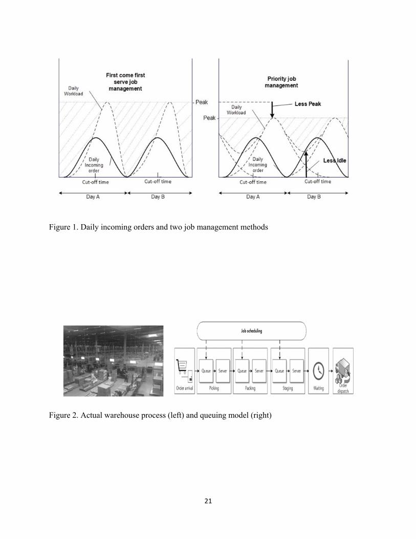
The balancing effect of job priority management is illustrated graphically in Figure 1. By

7
postponing part of the jobs stemming from demand peaks, the hourly workload becomes smoother
with less peaks and troughs compared to FCFS scheduling.
<< Insert Figure 1 about here. >>
Ideally, the workload should be constant across the day as this greatly simplifies warehouse
planning and operation. The incoming order arrival process is irregular so that this ideal situation
cannot be achieved in reality. We investigate the performance of alternative scheduling strategies
by a simulation study based on actual operational data of a case study warehouse. The methodology
to improve order fulfilment responsiveness for postponed cut-off times consists of four steps:
(1) Build a simulation model of order fulfilment that includes the following operational aspects:
arrival distributions, order peaks, due time distribution, service time distributions per operation,
and a set of priority rules to schedule remaining jobs for each queue.
(2) Construct a cost objective function that incorporates penalties for earliness, tardiness, idleness,
and work-in-process stock.
(3) Simulate the model under various cut-off scenarios and determine the costs resulting from each
priority rule.
(4) Evaluate the relative performance of these priority rules for the various scenarios and identify
which rule performs best under which circumstances.
For the case study warehouse, the simulation model of step (1) above has the following
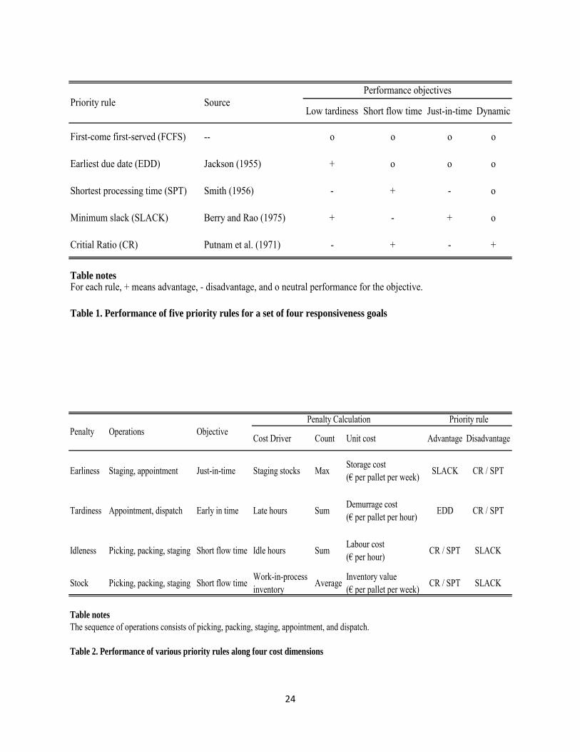
characteristics. The order fulfilment process consists of a tandem queue (Burke, 1956) with three
service stages: picking, where a pallet or box is moved from storage to the packing lane; packing,
where pallets are cubed according to customer requests; and staging, where pallets are moved from
the packing lane to the staging zone. Figure 2 shows this tandem queuing process, where the three
stages are linked without diversion and each stage consists of a set of servers with queues of
unlimited capacity. The number of workers is fixed per service but varies between picking, packing
and staging. Packing is the most labour intensive stage, with four workers per pallet. Packers
perform re-palletizing and wrapping tasks to satisfy customer warehouse pallet size restrictions
and they check that orders cubed as one pallet are complete before staging.
8
<< Insert Figure 2 about here. >>
As order arrival rates vary over the day, the arrival process at the picking stage is modelled
as a non-homogeneous Poisson process with varying rates per hour of the day. Service times are
modelled by simple exponential distributions with rates that differ for each of the three services of
picking, packing and staging. The service rates for picking and packing depend on the order type,
with a distinction between relatively simple single-item pallets (SIP) with faster rates and complex
multi-item pallets (MIP) with slower rates. For given service and order type, the service rate is
assumed to be constant per worker and per hour of the day. This assumption ignores ergonomic
factors like fatigue, but the warehouse employs a refined measurement system for labour
productivity per task per worker that indicates that this simplification is not unreasonable. All
workers are directed independently via WMS instructions transmitted by hand-held terminals and
they work per pallet without any knowledge of job priorities or shipment structures. The picking
process is modelled as an M(t)/M/c queue with non-homogeneous Poisson arrivals, packing
follows a G/M/c queuing model with arrivals determined by departures from upstream picking,
and staging also follows a G/M/c queuing model with arrivals determined by upstream packing.
The final phase of the order fulfilment process involves waiting, and the waiting time of pallets is
defined as the length of time they stay at the staging zone after packing and before shipping.
Historical warehouse operational data are used to specify the simulation input parameters
for hourly arrival rates (17, one for each hour of the working day from 6 am until 11 pm), service
rates (6, one for SIP and one for MIP for picking, packing and staging), and the mix of SIP and
MIP orders (with probability 0.77 for SIP and 0.23 for MIP). Due times are uniformly distributed
over the 17 hours of the next working day, because the OEM warehouse planned its agreements
with retailer warehouses to spread truck arrivals optimally over the day. Multiple orders from the
same client are consolidated and have the same due time to reduce transport costs.
9
4. Priority rules and performance criteria
The literature review mentioned some well-known priority rules for job scheduling from flow-
shop production theory, which will now be described in more detail. The simplest rule is first-
come first-served (FCFS), where jobs that arrive earlier get higher priority. The so-called earliest
due date (EDD) rule gives higher priority to jobs with earlier due time. Jackson (1955) proposed
this priority rule and showed that it minimizes the maximum of job tardiness. In our OEM
warehouse case study, the operational due time of dispatch by the carrier is already assigned upon
arrival of the order owing to pre-arrangements with the retailers placing the orders. Smith (1956)
proposed an alternative priority rule where jobs with shortest processing time (SPT) get highest
priority to get minimal mean flow time, that is, minimal work-in-process inventories. This result
is related to Little’s law (Little, 1961), which states that in steady state the mean number of units
in the system (L) equals the product of the mean arrival rate (λ) and the mean time the unit spent
in the system (W), so that L = λ×W. An opposite rule gives highest priority to jobs with longest
processing time (LPT). In our case study, processing times are defined in terms of the expected
total service time of all remaining operations, i.e., picking plus packing plus staging for the picking
queue; packing plus staging for the packing queue; and staging for the staging queue.
EDD and SPT focus on tardiness performance, but earliness and post-completion costs are
also relevant. Berry and Rao (1975) studied the slack time (SLACK) and critical ratio (CR) rules
to improve inventory performance. For given time (t), the slack time (St) of a job with due time
(D) is defined as the difference between remaining time (Dt = D – t) and (expected) remaining
processing time (Pt) with correction factor (c > 1) to account for expected queuing and other time
losses in the process, so that St = Dt – c×Pt. SLACK gives higher priority to jobs with less slack
time and constitutes a trade-off between EDD and LPT, as it assigns higher priority to jobs with
earlier due times that take longer to process. Berry and Rao (1975) showed that this rule averts
both inventory surpluses from early replenishment and inventory shortages from late supplier
deliveries. Similar to EDD and SPT, the SLACK priority of a job is static in the sense that all
priority parameters (due times and expected remaining processing times) are known upon arrival.
CR is a dynamic rule and replaces the correcting factor (c) by the expected queuing times that
apply during dynamic operation. This rule assigns highest priority to the job with the smallest
value of remaining time until due time (Dt = D – t) divided by the sum of expected remaining
processing time (Pt) and currently expected remaining queuing time (Qt), that is, (D – t)/(Pt + Qt).

10
Here Pt depends on the stage of the job; for example, at the packing stage it involves the expected
service times of packing and staging. Qt depends not only on the stage of the job, but also on the
queues it should still pass. These queues are dynamic and Qt depends on the expected processing
times of all unfinished jobs with higher priority. Putnam et al. (1971) reported that the CR rule
reduces uncertainty by trimming lateness variance. In general, CR is expected to perform better
than SLACK because it employs relevant extra dynamic information.
Table 1 provides a summary of the considered priority rules. EDD and SLACK reduce
tardiness but may result in longer flow times than the alternatives. SPT and CR aim for short flow
times but often lead or lag due dates with resulting weaker just-in-time and tardiness performance.
Both SLACK and CR leverage processing times to account for other factors. CR provides dynamic
corrections by means of “live” waiting times and is therefore expected to give shorter flow times
than SLACK.
<< Insert Table 1 about here. >>
Next we consider performance criteria to evaluate OEM warehouse operations. The
warehouse outcomes are evaluated in terms of a common cost criterion that integrates the four
objectives of low earliness, low tardiness, low labour idleness, and low work-in-process stocks.
The weight of each objective is determined by the associated penalty for failing to reach it, and
this cost structure will be case dependent. The cost criterion function for fulfilling a set of orders
is given by
Cost = ∑ 1 i 2 i 3 4 .
Here the symbols have the following meaning: ‘i’ denotes the order; ‘n’ is the total number of
orders; ‘αi’ is the earliness cost of job ‘i’ and involves space costs at the staging zone for awaiting
pick-up; ‘βi’ is the tardiness cost of the job and consists of demurrage costs for carriers from
appointed pick-up time until actual dispatch time; ‘ ’ is the total idleness cost, the sum total of
idle labour costs in the phases of picking, packing and staging; ‘ ’ is total work-in-process cost,
the sum over all ‘n’ jobs of financial costs from work-in-process inventories during picking,
11
packing, and staging; and ‘wi’ (i=1,2,3,4) are selection weights that determine which objectives
are incorporated (1 if yes and 0 if no), depending on the business environment.
The four objectives and expected performance of alternative priority rules are summarized
in Table 2. Earliness penalties favour just-in-time strategies like SLACK by reducing staging
buffer space, whereas CR and SPT exacerbate these penalties because of their shorter flow times.
Tardiness penalties favour strategies like EDD that prevent lateness. Even though CR and SPT
have shorter flow times, they tend to generate some very late jobs with large associated tardiness
penalties. If favourable business relationships between warehouses and truckers allow
rescheduling appointments without cost, then the tardiness penalty may be waived (w2=0). Idleness
and stock penalties, which are linked since curtailed stock-in-process requires less labour, are
related to lean production principles (Krafcik, 1988). The law L = λ×W of Little (1961) implies
that work-in-process inventories (L) and associated stock penalties are proportional to flow time
(W), so that CR and SPT are expected to perform well in this respect. However, if handled products
are relatively cheap so that inventory costs are negligible, then stock penalties could be discarded
(w4=0).
<< Insert Table 2 about here. >>
5. Simulation results
We investigate the cost performance of alternative job priority rules by a simulation study with
parameters derived from a case study OEM retail distribution centre of a multinational consumer
electronics manufacturer. Figure 3 summarizes the interactions of this distribution centre with its
manufacturer, sales department, retail warehouses and shops, carriers, and labour provider. The
order arrival process is determined by the sales department, and due times for order fulfilment are
agreed with carriers.
<< Insert Figure 3 about here. >>

12
The main question of interest is how to improve responsiveness for postponed daily order
cut-off times. Curve A in Figure 4 shows the historical hourly average order pattern for 2012-2014,
with steep demand peak just before the order cut-off time that was fixed at 2 pm during that period.
The simulation study considers postponed cut-off scenarios with cut-off time at 3 pm (B), 4 pm
(C), or 5 pm (D). The corresponding demand patterns are simply extrapolated by shifting the base
scenario (A) forwards in time while keeping the size of demand peaks and daily totals fixed.
<< Insert Figure 4 about here. >>
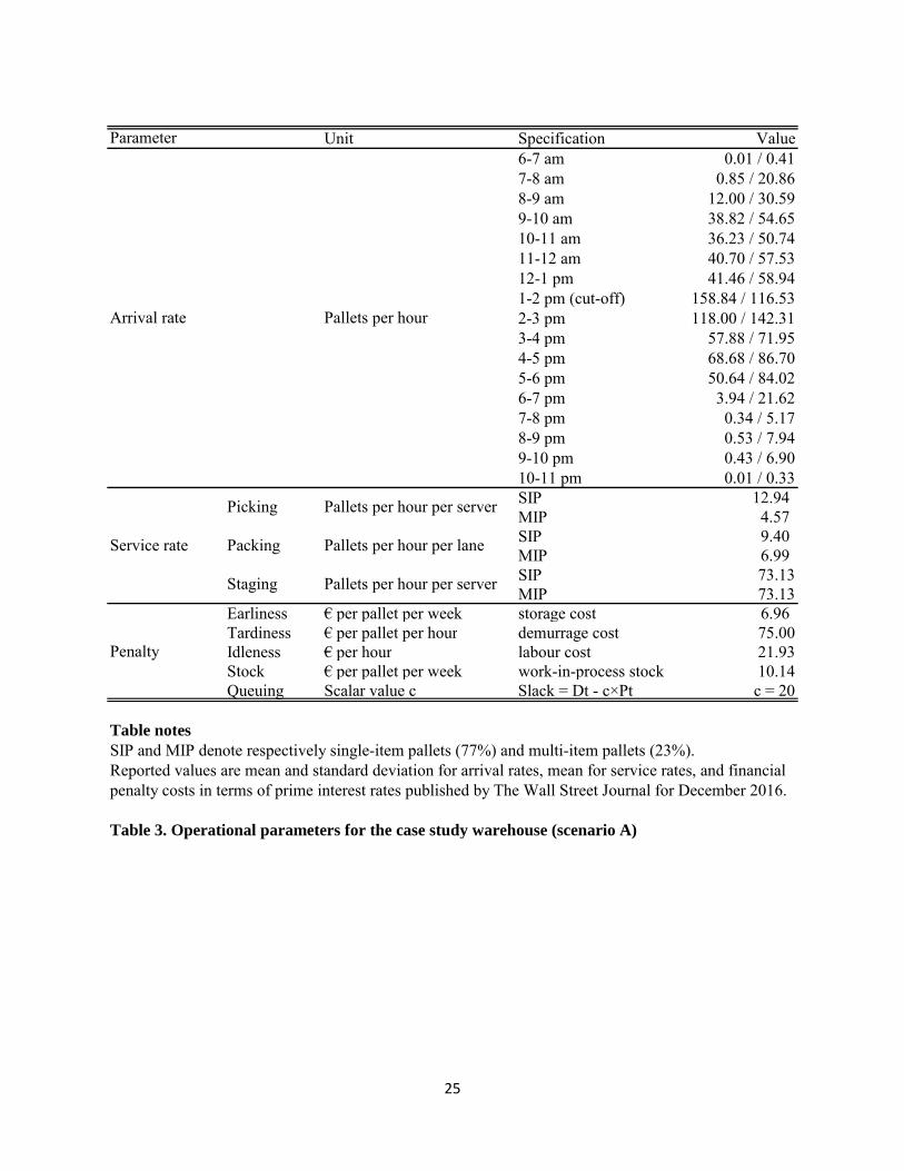
Table 3 summarizes the input parameters for the simulations derived from historical
operational data of the case study warehouse. The sales order desk is open from 8 am until 6 pm
and orders rarely arrive outside these hours, resulting in relatively small means and large standard
deviations of arrivals for out-of-office hours. Order arrivals have 77% chance to be SIP and 23%
to be MIP, and service rates for SIP are higher than those for MIP by factors 2.83 for picking and
1.34 for packing. Weekly idleness costs are obtained by multiplying the average non-utilisation
ratio by the weekly sum of total labour costs of €21.93 per hour. Stock-carrying costs are derived
from stock and space value and interest costs, with values per pallet per week of €10.14 for work-
in-process stocks and €6.96 for storage in the staging zone. Time criticality of order fulfilment for
this warehouse is shown by high demurrage costs of €75.00 per pallet per hour. Finally, for the
correction factor c in the definition of slack (St = Dt – c×Pt) we choose the same value (20) as in
the pilot study of FCFS by Kanet and Hayya (1982) to correct machine processing time for queuing
times. The average total processing time is 0.197 hours (1/12.94 + 1/9.40 + 1/73.13) for SIP and
0.376 hours (1/4.57 + 1/6.99 + 1/73.12) for MIP. This corresponds (for c = 20) to average
fulfilment durations of 20×0.197 = 3.9 hours for SIP and 20×0.376 = 7.5 hours for MIP, which
reasonably fits experiences in the case study warehouse
<< Insert Table 3 about here. >>

13
Every single simulation run corresponds to one week of warehouse operations with hourly
order arrivals, order types, and order service times. A week consists of five days of 17 hours each
(85 hours in total) with expected total arrival orders of around 3,200 pallets. One common set of
1,000 simulation runs is employed to study the outcomes of the five considered priority rules for
each of the four cut-off scenarios (A-D). Each of these twenty scenarios is evaluated in terms of
operational performance. The flow time of a job is the total time it spends in the shop, that is, the
time elapsing between arrival and completion. Lateness is defined as the difference between
completion time and due time, so that negative values correspond to timely completion. For
smooth operation it is preferred to have not only small mean but also small variation of flow times
and lateness, so that we consider both the mean and the standard deviation of these two
characteristics across the set of jobs within a given simulation run, that is, a given week of
warehouse operations. Tardiness occurs if lateness is positive, that is, if jobs are completed after
the due time limit. Maximum tardiness is defined as the maximum value of (positive) lateness
across all jobs within a given simulation run.
The operational outcomes of 1,000 simulation runs (weeks of order fulfilment) are
summarized in Table 4 and Figure 5. Table 4 shows that postponed cut-off times lead, as expected,
to shorter flow times, less lateness and more tardiness. FCFS does not perform well across all
performance dimensions and has the worst tardiness outcomes, especially for tight cut-off
scenarios. Of the five priority rules, CR performs by far the best in terms of flow time, whereas
EDD and SLACK have excellent tardiness results as none of their jobs have positive lateness.
Figure 5 shows some outlying tardiness results for CR, both in the benchmark cut-off scenario (A,
2 pm) and in the most ambitious scenario (D, 5 pm). SLACK and EDD perform roughly similar,
but because SLACK amplifies the weight of processing times it has smallest lateness and longest
flow times of all priority rules. Compared to these two methods, SPT has shorter flow times but
more tardiness. The outcomes in Table 4 are in line with those in Table 1, because CR and SPT
have shortest flow times, EDD and SLACK have lowest tardiness, and SLACK comes closest to
just-in-time planning as it has highest lateness.
<< Insert Table 4 and Figure 5 about here. >>

14
Table 5 summarizes the financial outcomes of the simulation experiments. These outcomes
consist of costs associated with earliness, tardiness, idleness, and stock costs. We consider an
integrated cost function that includes all four cost components as well as two restricted versions.
One version excludes stock costs, which is relevant for warehouses at urban locations with just-
in-time planning that have relatively low stock value compared to high storage rental costs.
Another version excludes tardiness costs for warehouses that handle high-priced goods with high
storage rental costs and that have flexible pick-up agreements with carriers to skip tardiness
penalties. EDD performs best if all components are included, SLACK is best if there are no stock
costs, and CR is best if there are no tardiness costs. These rankings of priority rules do not depend
on the cut-off scenario and get more pronounced for tighter scenarios. In scenario A (2 pm), the
percentage of simulation runs for which EDD, SLACK and CR are optimal are respectively 46.5,
48.1, and 56.6, and for scenario D these percentages are respectively 93.7, 66.6, and 59.4. The
outcomes illustrate that there is no priority rule that is universally best for all business situations,
but each warehouse may find a suitable rule by selecting the performance objectives that apply for
its specific situation.
<< Insert Table 5 about here. >>
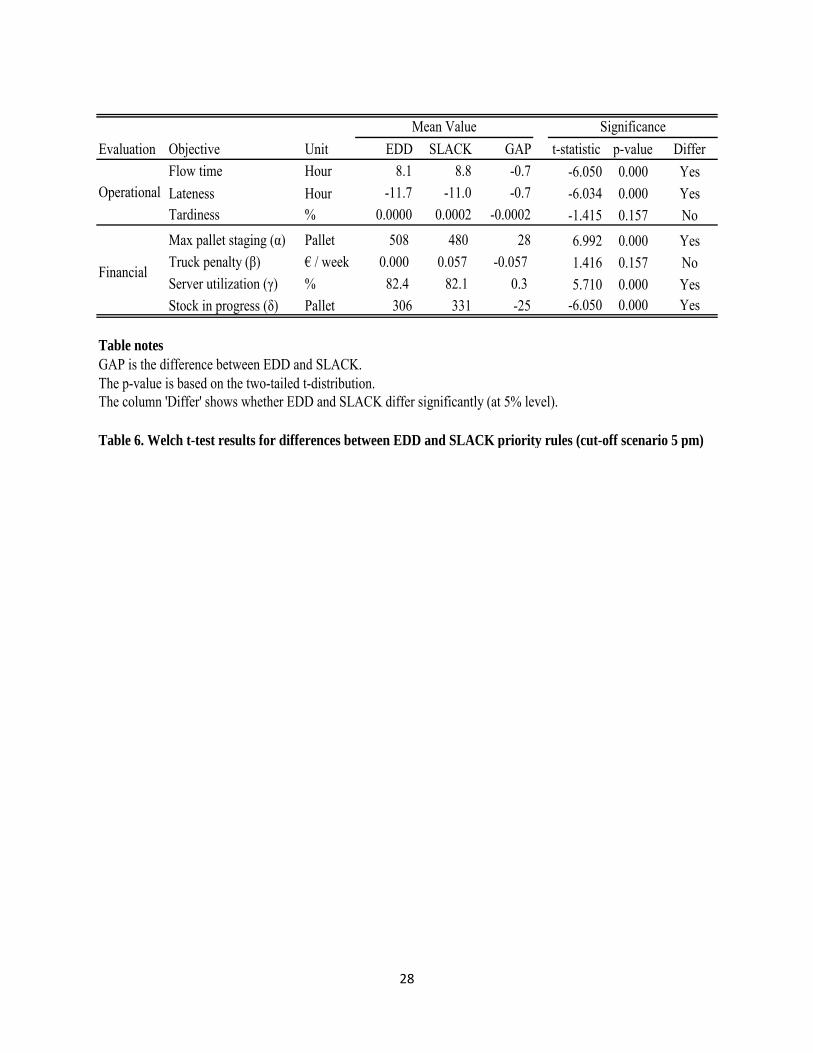
As EDD and SLACK perform roughly similar, we provide a more detailed comparison of these
two rules by means of paired t-tests (Welch, 1947) for operational and financial performance for
the tightest cut-off scenario (D, 5 pm). The sample size of 1,000 runs far exceeds the usual rule-
of-thumb threshold (30) so that we employ the conventional standard normal distribution to
compute p-values. The results in Table 6 show significant differences between the two methods.
In terms of operational performance, SLACK is more just-in-time and EDD has shorter flow time.
From a financial perspective, SLACK requires less staging space but EDD has higher server
utilization and less work-in-process stocks. The two rules do not show significant differences in
tardiness and associated demurrage costs.
<< Insert Table 6 about here. >>

15
6. Some operational implications and conclusions
Enhanced competitiveness in retail markets asks for higher levels of responsiveness to satisfy
consumer expectations. OEM warehouses, for example, can improve their order delivery speed by
postponing order cut-off times for next-day delivery. To smoothen warehouse operations for
efficient resource allocation, priority rules help in sequencing outstanding jobs at various stages of
the warehouse process. The choice which rule to apply depends on the objectives and cost structure
of the warehouse. The methodology proposed in this paper suggests careful examination of the
business environment to identify relevant performance objectives and cost parameters. Historical
operational warehouse data can be used to model the stochastic nature of the order arrival process
and of the service and queuing times for the various stages of the outbound warehouse process.
In our analysis we distinguished performance along four dimensions by preventing
earliness (staging costs), tardiness (demurrage costs), idleness (labour costs), and work-in-process
inventories (stock costs). It depends on the business environment which of these dimensions are
actually relevant. Preventing tardiness, for example, is imperative if delayed delivery spoils all
product virtues, whereas it is less relevant if delays can be solved by penalty-free rescheduling of
pick-up times. The latter situation often applies for OEM warehouses that deliver to retailer
warehouses and shops. Our simulation results show that the critical ratio (CR) priority rule
performs well in such situations. It offers shortest flow time with fewest work-in-process stock,
which is valuable for businesses that handle expensive products with high labour costs.
The case study warehouse currently uses the earliest due date (EDD) strategy for
sequencing its order fulfilment jobs. The simulation results based on the warehouse-specific cost
parameters indicate potential benefits of the CR rule. Compared to the other priority rules, CR has
the unique property that it incorporates the dynamic queuing status of jobs in determining their
priority. The simulation study employs a rough estimate of queuing times based on expected
processing times of jobs with higher priority. These estimates could be refined by studying actual
workflow patterns and queuing data from the warehouse process and by forecasting queuing times
using statistical and machine learning methods. The case study warehouse is interested in refining
the job scheduling strategy in its WMS.

16
Summarizing the contributions of this paper, the current retail market leverages
responsiveness of order fulfilment and forces higher levels of efficiency in distribution. From
this perspective, job scheduling using flow-shop priority rules offers solutions for distribution
centres facing cut-off time pressures. By prioritising each job, warehouses can efficiently maintain
responsiveness without increasing labour to satisfy compressed order-fulfilment deadlines. The
paper presents a simulation-based methodology for selecting priority rules by evaluating
alternative rules in terms of composite cost objectives that can be tailored to warehouse-specific
settings. Simulation results indicate good performance of the SLACK rule for just-in-time
operations with high storage costs and of the CR rule for high-value product operations with
flexible pick-up schedules.
Further research is needed to analyse the trade-off between potential revenue gains through
better service with postponed cut-off times against increased costs due to tighter processing
conditions. It is also of interest to study historical workflow patterns in more detail to refine CR-
type priority rules by improving forecasts of remaining processing and queuing times.
References
Baker, K.R., and G.D. Scudder. 1990. “Sequencing with earliness and tardiness penalties: A
review.” Operations Research 38 (1): 22–36.
Barclay, I., J. Poolton, and Z. Dann. 1996. “Improving competitive responsiveness via the virtual
environment.” In Engineering and Technology Management, IEMC 96, IEEE Proceedings,
52–62.
Bartholdi III, J.J., and S.T. Hackman. 2011. Warehouse & Distribution Science: Release 0.92.
Atlanta, GA, The Supply Chain and Logistics Institute, School of Industrial and Systems
Engineering, Georgia Institute of Technology.
Bartholdi III, J.J., D.D. Eisenstein, and R.D. Foley. 2001. “Performance of bucket brigades when
work is stochastic.” Operations Research 49 (5), 710-719.
Berry, W.L., and V. Rao. 1975. “Critical ratio scheduling: An experimental analysis.”
Management Science 22 (2): 192–201.
17
Burke, P.J. 1956. “The output of a queuing system.” Operations Research 4(6), 699-704.
Cakici, E., S.J. Mason, and M.E. Kurz. 2012. “Multi-objective analysis of an integrated supply
chain scheduling problem.” International Journal of Production Research 50 (10): 2624–
2638.
Chen, C. M., Y. Gong, R. De Koster, and J.A. Van Nunen. 2010. “A flexible evaluative framework
for order picking systems.” Production and Operations Management 19(1), 70-82.
De Koster, M.D., and B.M. Balk. 2008. “Benchmarking and monitoring international warehouse
operations in Europe.” Production and Operations Management 17(2), 175-183.
De Koster, R.B., T. Le-Duc, and K.J. Roodbergen. 2007. “Design and control of warehouse order
picking: A literature review.” European Journal of Operational Research 182 (2): 481–
501.
De Koster, R.B., T. Le-Duc, and N. Zaerpour. 2012. “Determining the number of zones in a pick-
and-sort order picking system.” International Journal of Production Research 50(3), 757-
771.
De Leeuw, S., and V.C. Wiers. 2015. “Warehouse manpower planning strategies in times of
financial crisis: Evidence from logistics service providers and retailers in the Netherlands.”
Production Planning & Control 26 (4): 328–337.
Denman, T. 2017. “The omni channel supply chain: From the docks to the doorstep.” Available
at: https://risnews.com/omnichannel-supply-chain-docks-doorstep (accessed 4 July 2017).
Doerr, K.H., and K.R. Gue. 2013. “A performance metric and goal‐setting procedure for deadline
oriented processes.” Production and Operations Management 22 (3): 726–738.
Elsayed, E.A., M.K. Lee, S. Kim, and E. Scherer. 1993. “Sequencing and batching procedures for
minimizing earliness and tardiness penalty of order retrievals.” International Journal of
Production Research 31 (3): 727–738.
Freiheit, T., and L. Wei. 2016. “The effect of work content imbalance and its interaction with
scheduling method on sequential flow line performance.” International Journal of
Production Research 55 (10): 2791–2805.

18
Gong, Y., and R.B. De Koster. 2011. “A review on stochastic models and analysis of warehouse
operations.” Logistics Research 3 (4): 191-205.
Graves, S.C., W.H. Hausman, and L.B. Schwarz. 1977. “Storage-retrieval interleaving in
automatic warehousing systems.” Management Science 23 (9): 935-945.
Hackman, S.T., E.H. Frazelle, P.M. Griffin, S.O. Griffin, and D.A. Vlasta. 2001. “Benchmarking
warehousing and distribution operations: an input-output approach.” Journal of
Productivity Analysis 16(1), 79-100.
Hall, R.W. 1993. “Distance approximations for routing manual pickers in a warehouse.” IIE
Transactions 25 (4): 76–87.
Huang, H.C., C. Lee, and Z. Xu. 2006. “The workload balancing problem at air cargo terminals.”
OR Spectrum 28 (4): 705–727.
Jackson, J.R. 1955. Scheduling a Production Line to Minimize Maximum Tardiness. Numerical
Analysis Research, University of California, Los Angeles.
Jarvis, J.M., and E.D. McDowell. 1991. “Optimal product layout in an order picking warehouse.”
IIE Transactions 23 (1): 93–102.
Johnson, S.M. 1954. “Optimal two‐and three‐stage production schedules with setup times
included.” Naval Research Logistics Quarterly 1 (1): 61–68.
Kanet, J.J., and J.C. Hayya. 1982. “Priority dispatching with operation due dates in a job shop.”
Journal of Operations Management 2 (3): 167–175.
Kemppainen, K. 2005. Priority Scheduling Revisited – Dominant Rules, Open Protocols, and
Integrated Order Management. PhD Thesis A-261, Helsinki School of Economics.
Kiran, A.S., and M.L. Smith. 1984. “Simulation studies in job shop scheduling - a survey.”
Computers & Industrial Engineering 8 (2): 87–93.
Krafcik, J.F. 1988. “Triumph of the lean production system.” MIT Sloan Management Review 30
(1): 41.
19
Kritchanchai, D., and B.L. MacCarthy. 1999. “Responsiveness of the order fulfilment process.”
International Journal of Operations & Production Management 19 (8): 812–833.
Lee, C.Y., S. Piramuthu, and Y.K. Tsai. 1997. “Job shop scheduling with a genetic algorithm and
machine learning.” International Journal of Production Research 35 (4): 1171–1191.
Little, J.D.C. 1961. “A proof for the queuing formula: L=λW.” Operations Research 9 (3): 383–
387.
Pagh, J.D., and M.C. Cooper. 1998. “Supply chain postponement and speculation strategies: How
to choose the right strategy.” Journal of Business Logistics 19 (2): 13.
Pearcy, M., and B. Kerr. 2013. “From customer orders through fulfilment: Challenges and
opportunities in manufacturing, high-tech and retail.” Available at:
https://www.fi.capgemini.com/from-customer-orders-through-fulfilment-challenges-and-
opportunities (accessed 4 July 2017)
Petersen, C.G. 1997. “An evaluation of order picking routing policies.” International Journal of
Operations and Production Management 17 (11): 1098–1111.
Petersen, C.G. 2000. “An evaluation of order picking policies for mail order companies.”
Production and Operations Management 9 (4): 319–335.
Petersen, C.G., G.R. Aase, and D.R. Heiser. 2004. “Improving order-picking performance through
the implementation of class-based storage.” International Journal of Physical Distribution
& Logistics Management 34 (7): 534–544.
Putnam, A.O., R. Everdell, G.H. Dorman, R.R. Cronan, and L.H. Lindgren. 1971. “Updating
critical ratio and slack time priority scheduling rules.” Production and Inventory
Management 12 (4): 41–73.
Ramaa, A., K.N. Subramanya, and T.M. Rangaswamy. 2012. “Impact of warehouse management
system in a supply chain.” International Journal of Computer Applications 54 (1), 14-20.
Ramasesh, R., 1990. “Dynamic job shop scheduling: A survey of simulation research.” Omega 18
(1): 43–57.

20
Roodbergen, K.J., and R. De Koster. 2001. “Routing methods for warehouses with multiple cross
aisles.” International Journal of Production Research 39 (9): 1865–1883.
Shaw, A., D.C. McFarlane, Y.S. Chang, and P.J.G. Noury. 2003. “Measuring response capabilities
in the order fulfilment process.” In Proceedings of EUROMA, Como, Italy.
Smith, W.E. 1956. “Various optimizers for single stage production.” Naval Research Logistics
Quarterly 3 (1–2): 59–66.
T’kindt, V. 2011. “Multicriteria models for just-in-time scheduling.” International Journal of
Production Research 49 (11): 3191–3209.
T’kindt, V., and J.C. Billaut. 2006. Multicriteria Scheduling. Theory, Model, and Algorithms.
Heidelberg: Springer.
Treleven, M.D., and D.A. Elvers. 1985. “An investigation of labour assignment rules in a dual-
constrained job shop.” Journal of Operations Management 6 (1): 51–68.
Van den Berg, J.P. 1999. “A literature survey on planning and control of warehousing systems.”
IIE Transactions 31 (8): 751–762.
Van den Berg, J.P. 2007. Integral Warehouse Management. Utrecht: Management Outlook.
Van Nieuwenhuyse, I., and R.B. De Koster. 2009. “Evaluating order throughput time in 2-block
warehouses with time window batching.” International Journal of Production Economics
121(2), 654-664.
Welch, B.L. 1947. “The generalization of ‘Student’s’ problem when several different population
variances are involved.” Biometrika 34 (1/2): 28–35.
Won, J., and S. Olafsson. 2005. “Joint order batching and order picking in warehouse operations.”
International Journal of Production Research 43 (7): 1427–1442.
21
Figure 1. Daily incoming orders and two job management methods
Figure 2. Actual warehouse process (left) and queuing model (right)

22
Figure 3. Retail distribution centre (OEM warehouse) and SCM partners
Figure 4. Average hourly incoming orders per for four cut-off scenarios (current is A)

23
Figure 5. Histograms of simulated outcomes for lateness (0 on horizontal axis means -4.99 to 0.00)
24
Low tardiness Short flow time Just-in-time Dynamic
First-come first-served (FCFS) -- o o o o
Earliest due date (EDD) Jackson (1955) + o o o
Shortest processing time (SPT) Smith (1956) - + - o
Minimum slack (SLACK) Berry and Rao (1975) + - + o
Critial Ratio (CR) Putnam et al. (1971) - + - +
Table notes
Table 1. Performance of five priority rules for a set of four responsiveness goals
For each rule, + means advantage, - disadvantage, and o neutral performance for the objective.
Priority rule SourcePerformance objectives
Cost Driver Count Unit cost Advantage Disadvantage
Earliness Staging, appointment Just-in-time Staging stocks MaxStorage cost(€ per pallet per week)
SLACK CR / SPT
Tardiness Appointment, dispatch Early in time Late hours SumDemurrage cost (€ per pallet per hour)
EDD CR / SPT
Idleness Picking, packing, staging Short flow time Idle hours SumLabour cost(€ per hour)
CR / SPT SLACK
Stock Picking, packing, staging Short flow timeWork-in-process inventory
AverageInventory value(€ per pallet per week)
CR / SPT SLACK
Table notesThe sequence of operations consists of picking, packing, staging, appointment, and dispatch.
Table 2. Performance of various priority rules along four cost dimensions
ObjectivePriority rulePenalty Calculation
Penalty Operations
25
Unit Specification Value6-7 am 0.01 / 0.417-8 am 0.85 / 20.868-9 am 12.00 / 30.599-10 am 38.82 / 54.6510-11 am 36.23 / 50.7411-12 am 40.70 / 57.5312-1 pm 41.46 / 58.941-2 pm (cut-off) 158.84 / 116.532-3 pm 118.00 / 142.313-4 pm 57.88 / 71.954-5 pm 68.68 / 86.705-6 pm 50.64 / 84.026-7 pm 3.94 / 21.627-8 pm 0.34 / 5.178-9 pm 0.53 / 7.949-10 pm 0.43 / 6.9010-11 pm 0.01 / 0.33SIP 12.94 MIP 4.57 SIP 9.40 MIP 6.99 SIP 73.13MIP 73.13
Earliness € per pallet per week storage cost 6.96 Tardiness € per pallet per hour demurrage cost 75.00Idleness € per hour labour cost 21.93Stock € per pallet per week work-in-process stock 10.14Queuing Scalar value c Slack = Dt - c×Pt c = 20
Table notes
Arrival rate
Parameter
Pallets per hour
Reported values are mean and standard deviation for arrival rates, mean for service rates, and financialpenalty costs in terms of prime interest rates published by The Wall Street Journal for December 2016.
Table 3. Operational parameters for the case study warehouse (scenario A)
SIP and MIP denote respectively single-item pallets (77%) and multi-item pallets (23%).
Pallets per hour per server
Pallets per hour per lane
Pallets per hour per server
Penalty
Service rate
Picking
Packing
Staging

26
Cut-off Priority mean std mean std mean std mean std mean std mean stdFCFS 8.7 2.3 2.9 0.2 -16.6 2.3 7.2 0.2 2.6 2.5 1.1 1.5SPT 7.3 2.1 5.0 0.7 -18.0 2.1 6.9 0.2 2.3 2.4 0.6 0.8EDD 8.7 2.3 6.9 1.0 -16.6 2.3 3.2 1.0 0.0 0.0 0.0 0.0SLACK 9.3 2.4 7.2 0.9 -16.0 2.4 3.3 0.9 0.0 0.0 0.0 0.0CR 4.8 0.5 6.9 2.2 -19.9 0.6 6.8 1.5 33.7 24.4 1.0 0.8
FCFS 8.5 2.2 2.9 0.2 -14.9 2.2 7.2 0.3 3.9 2.8 2.2 2.5SPT 7.1 2.0 5.2 0.7 -16.4 2.0 6.9 0.2 3.6 2.7 1.1 1.4EDD 8.5 2.2 7.0 0.9 -15.0 2.2 3.0 1.1 0.0 0.0 0.0 0.0SLACK 9.2 2.3 7.3 0.9 -14.3 2.3 3.2 0.9 0.0 0.0 0.0 0.0CR 4.5 0.6 6.9 2.3 -18.3 0.6 6.7 1.5 35.2 23.2 1.1 0.8
FCFS 8.4 2.3 2.8 0.2 -13.0 2.3 7.3 0.2 5.8 2.9 4.5 4.0SPT 6.9 2.1 5.1 0.6 -14.5 2.2 6.9 0.2 5.5 2.9 2.4 2.4EDD 8.4 2.3 7.0 0.9 -13.1 2.3 2.8 1.1 0.0 0.0 0.0 0.0SLACK 9.0 2.4 7.2 0.8 -12.4 2.4 3.0 0.9 0.0 0.0 0.0 0.0CR 4.3 0.6 6.8 2.4 -16.4 0.7 6.6 1.6 36.0 25.5 1.1 0.9
FCFS 8.1 2.4 2.7 0.3 -11.7 2.4 7.2 0.2 7.0 3.1 6.8 5.2SPT 6.6 2.3 4.8 0.5 -13.2 2.3 6.9 0.2 6.7 3.1 3.9 3.3EDD 8.1 2.4 6.7 0.8 -11.7 2.4 2.7 1.1 0.0 0.0 0.0 0.0SLACK 8.8 2.5 7.0 0.7 -11.0 2.5 2.9 0.9 0.0 0.0 0.0 0.0CR 4.1 0.6 7.0 2.4 -15.0 0.7 6.5 1.6 37.7 25.2 1.2 0.8
Underscored mean values are for the best performing priority rule per objective and per cut-off scenario.Flow time, lateness and tardiness are measured in hours, and fraction of tardiness is measured as percentage.The standard deviation columms (std) show the variation of outcomes across the 1,000 simulation runs.
Table 4. Simulated performance of five priority methods
TardinessMaximum Fraction (%)
Table notes
Flow timeMean Standard dev.Mean
5 pm
Standard dev.
2 pm
3 pm
4 pm
Lateness

27
Obj
ectiv
eSt
ock
(δ)
Mea
sure
men
tPi
ckPa
ckSt
age
Tota
l A
vera
gePa
llet
Cut-o
ffPr
iorit
ym
ean
std
mea
nstd
mea
n st
d be
st (%
) m
ean
std
best
(%)
mea
n st
d be
st (%
)
FCFS
687
804,
708
8,24
297
.281
.248
.282
.432
7.4
22,0
5611
,546
0.1
18,6
5710
,882
9.4
16,3
2389
00.
1SP
T71
282
2,35
04,
220
97.2
81.7
48.6
82.8
274.
9
18
,687
6,39
646
.615
,831
5,80
72.
715
,766
794
43.3
2 pm
EDD
687
810.
000.
0097
.281
.248
.282
.432
7.0
16,3
2489
346
.512
,927
557
39.7
16,3
2489
30.
0SL
ACK
668
860.
000.
0097
.280
.948
.082
.235
1.5
16,5
7191
60.
012
,922
570
48.1
16,5
7191
60.
0
CR78
231
47,8
4157
,230
97.2
80.6
47.8
82.0
179.
4
61
,648
52,6
896.
859
,826
52,4
990.
115
,678
633
56.6
FCFS
629
7911
,070
18,0
8097
.381
.148
.282
.432
2.4
27,3
3018
,948
0.0
24,0
5418
,266
3.1
15,7
9186
00.
0SP
T65
767
5,61
49,
769
97.3
81.7
48.7
82.9
268.
1
21
,056
10,3
6026
.218
,334
9,75
83.
315
,203
811
48.1
3 pm
EDD
629
800.
000.
0097
.381
.148
.282
.432
1.6
15,7
8085
769
.412
,515
581
40.4
15,7
8085
70.
0SL
ACK
607
870.
000.
0097
.380
.747
.982
.134
6.2
16,0
2487
50.
012
,508
596
53.2
16,0
2487
50.
0
CR72
629
50,0
2362
,785
97.3
80.5
47.8
81.9
170.
9
62
,125
55,6
794.
460
,394
55,4
950.
015
,121
600
51.9
FCFS
561
8226
,973
33,2
7497
.281
.248
.382
.431
6.6
45,4
2435
,018
0.0
42,0
8834
,249
0.4
15,3
6692
50.
0SP
T60
752
14,2
2218
,379
97.2
82.1
49.0
83.2
260.
9
30
,480
19,6
756.
827
,718
18,9
730.
414
,799
925
42.9
4 pm
EDD
561
830.
000.
0097
.281
.248
.382
.531
5.9
15,3
4792
887
.312
,018
601
35.0
15,3
4792
80.
0SL
ACK
535
890.
010.
2597
.280
.848
.082
.134
0.9
15,5
8394
90.
111
,994
610
64.2
15,5
8394
90.
0
CR65
731
53,6
9470
,056
97.2
80.7
47.9
82.1
163.
9
64
,066
66,4
565.
862
,415
66,2
540.
014
,610
644
57.1
FCFS
509
8545
,756
48,2
9597
.281
.248
.382
.430
7.0
63,7
5748
,231
0.0
60,5
5947
,444
0.0
14,8
6592
60.
0SP
T57
255
24,7
3227
,716
97.2
82.2
49.1
83.3
250.
1
40
,158
27,7
330.
837
,544
27,0
160.
014
,335
951
40.6
5 pm
EDD
508
870.
000.
0097
.281
.248
.382
.430
5.5
14,8
4891
293
.711
,661
563
32.9
14,8
4891
20.
0SL
ACK
480
890.
061.
2797
.280
.847
.982
.133
0.8
15,1
641,
709
0.1
11,7
151,
393
66.6
15,0
8094
10.
0
CR60
433
60,8
7768
,854
97.2
80.8
47.9
82.1
155.
8
75
,991
65,7
105.
474
,406
65,5
170.
514
,116
644
59.4
Idle
ness
cos
ts ar
e fo
r ope
ratio
n w
ith 2
5 w
orke
rs: 4
pic
kers
, 5 p
acki
ng la
nes w
ith in
tota
l 20
pack
ers,
and
1 sta
ger.
Bes
t (%
) sho
ws t
he p
erce
ntag
e of
all
1,00
0 sim
ulat
ion
runs
whe
re th
is pr
iorit
y ru
le h
as lo
wes
t cos
t acr
oss t
he fi
ve c
onsi
dere
d ru
les.
The
stand
ard
devi
atio
n co
lum
ms (
std) s
how
the
varia
tion
of o
utco
mes
acr
oss t
he 1
,000
sim
ulat
ion
runs
.
Tabl
e 5.
Sim
ulat
ion
outc
omes
of f
ive
prio
rity
rul
es fo
r th
ree
cust
omiz
ed p
erfo
rman
ce c
rite
ria
Max
. sta
ge
Truc
k pe
nalty
€€
€
Earli
ness
(α)
Tard
ines
s (β)
Idle
ness
(γ)
Cos
t spe
cific
atio
n
All
four
(α +
β +
γ +
δ)
No
stock
cos
t (α
+ β
+ γ)
N
o ta
rdin
ess c
ost (α
+ γ
+ δ)
€Pa
llet
Util
izat
ion
(%)
Uni
t
Tabl
e no
tes
28
Evaluation Objective Unit EDD SLACK GAP t-statistic p-value Differ
Flow time Hour 8.1 8.8 -0.7 -6.050 0.000 Yes
Lateness Hour -11.7 -11.0 -0.7 -6.034 0.000 YesTardiness % 0.0000 0.0002 -0.0002 -1.415 0.157 No
Max pallet staging (α) Pallet 508 480 28 6.992 0.000 YesTruck penalty (β) € / week 0.000 0.057 -0.057 1.416 0.157 NoServer utilization (γ) % 82.4 82.1 0.3 5.710 0.000 YesStock in progress (δ) Pallet 306 331 -25 -6.050 0.000 Yes
GAP is the difference between EDD and SLACK.The p-value is based on the two-tailed t-distribution.The column 'Differ' shows whether EDD and SLACK differ significantly (at 5% level).
Table 6. Welch t-test results for differences between EDD and SLACK priority rules (cut-off scenario 5 pm)
Table notes
Financial
Mean Value
Operational
Significance
Top Related