


Languages
Pages
Legal


IMPERIAL COLLEGE LONDON
Department of Earth Science and Engineering
Centre for Petroleum Studies
Reducing Fluid Type Uncertainty with Well Test Analysis
By
Hidayat Abd Hir
A report submitted in partial fulfilment of the requirements for
the MSc and/or the DIC
September 2011

Reducing fluid type uncertainty with Well Test Analysis ii
ii
DECLARATION OF OWN WORK
I declare that this thesis “Reducing fluid type uncertainty with well test analysis” is entirely my own
work and that where any material could be construed as the work of others, it is fully cited and
referenced, and /or with appropriate acknowledgements given.
Signature: ………………………………………………………………………………………..
Name of student: Hidayat Abd Hir
Name of Imperial College supervisor: Prof. Alain C. Gringarten
Name of Industry supervisor: Dr. Peyman Nurafza, Eon Ruhrgas UK Limited

Reducing fluid type uncertainty with Well Test Analysis iii
ACKNOWLEDGEMENT
I would like to thank E.ON Ruhrgas UK E&P Limited for providing the opportunity to carry on this project, and the
permission to present the results.
I would like to express my deepest gratitude to Professor Alain C. Gringarten for his support and clear guidance
throughout the project, and Olakunle Ogunrewo for his help, suggestions, encouragement during the project. My appreciation
also goes to Dr. Peyman Nurafza (E.ON Ruhrgas) for providing data and guidance throughout the project.
Special thanks to MARA for providing me with a scholarship to pursue my studies at Imperial College London.
I also wish to thank to all my friends at Imperial College London for the memorable time shared during the course.
Finally, I dedicate this work to my family for their support and encouragement throughout my studies.

Reducing fluid type uncertainty with Well Test Analysis iv
iv
TABLE OF CONTENTS
DECLARATION OF OWN WORK............................................................................................................................................. ii
ACKNOWLEDGEMENT ........................................................................................................................................................... iii
TABLE OF CONTENTS ............................................................................................................................................................. iv
LIST OF FIGURES .......................................................................................................................................................................v
LIST OF TABLES .........................................................................................................................................................................v
Abstract ..........................................................................................................................................................................................1
Introduction ....................................................................................................................................................................................1
Introduction to the field ..................................................................................................................................................................3
Available information ....................................................................................................................................................................4
Methodology and data analyses .....................................................................................................................................................5
PVT modelling ...........................................................................................................................................................................5
Well Test Analysis .....................................................................................................................................................................6
Data preparations ................................................................................................................................................................... 6
Deconvolution – initial reservoir pressure ............................................................................................................................. 7
Principal of deconvolution – rate corrections ........................................................................................................................ 8
Deconvolution – well test interpretation model..................................................................................................................... 8
2-phase pseudo-pressure analysis .......................................................................................................................................... 9
Results and discussion ................................................................................................................................................................. 11
Conclusion ................................................................................................................................................................................... 12
Recommendations ........................................................................................................................................................................ 12
Nomenclature ............................................................................................................................................................................... 13
Subscripts ..................................................................................................................................................................................... 13
Greek ............................................................................................................................................................................................ 13
References .................................................................................................................................................................................... 13
APPENDIX A .............................................................................................................................................................................. 15
Critical Literature Review ........................................................................................................................................................ 15
APPENDIX B .............................................................................................................................................................................. 19
Geology illustration of the field ............................................................................................................................................... 19
APPENDIX C .............................................................................................................................................................................. 20
APPENDIX D .............................................................................................................................................................................. 23
Well test interpretation model .................................................................................................................................................. 23
APPENDIX E .............................................................................................................................................................................. 24
Well test interpretation for volatile oil case ............................................................................................................................. 24
APPENDIX F ............................................................................................................................................................................... 25
Well test interpretation for gas condensate case ....................................................................................................................... 25

Reducing fluid type uncertainty with Well Test Analysis v
LIST OF FIGURES Figure 1: Schematic of single-phase pseudo-pressure and derivative three-region (a) and two-region (b) composite behavior
(Gringarten et al., 2000) .................................................................................................................................................................3 Figure 2: Single-phase versus two-phase pseudo-pressure formulation (Gringarten et al., 2006) .................................................3 Figure 3: Phase envelope for each reservoir fluid sample ..............................................................................................................5 Figure 4: Bottom-hole sample comparison of EOS model with CCE experiment .........................................................................5 Figure 5: Low GOR recombined sample comparison of EOS model with CCE experiment .........................................................6 Figure 6: Pressure and rate data history from DST ........................................................................................................................6 Figure 7: Rate validation of pressure build ups from DST............................................................................................................6 Figure 8: Initial pressure determination for both gas condensate and volatile oil cases.................................................................7 Figure 9: Entire pressure match for gas condensate .......................................................................................................................7 Figure 10: Entire pressure match for volatile oil ............................................................................................................................7 Figure 11: Rate corrections for gas condensate ..............................................................................................................................8 Figure 12: Rate corrections for volatile oil ....................................................................................................................................8 Figure 13: Interpretation model for unit pressure drawdown for gas condensate case ..................................................................9 Figure 14: Single and two-phase pseudo-pressure log-log plot for gas condensate for FP 76 (PBU 3) ....................................... 10 Figure 15: Two-phase pseudo-pressure log-log plot for volatile oil for FP 76 (PBU 3) .............................................................. 10 Figure 16: Well test analysis for FP 76 - PBU 3 (volatile oil case)............................................................................................. 10 Figure 17: Wellbore skin vs. rate for gas condensate case ........................................................................................................... 11 Figure 18: Wellbore skin vs. rate for volatile oil case .................................................................................................................. 11 Figure 19: Wellbore skin vs. rate for both gas condensate and volatile oil cases ........................................................................ 11
Figure B 1: Hydrocarbon accumulation system in the field under study ..................................................................................... 19
Figure C 1: Comparison of EOS predicted and observed values from CCE experiment for bottom-hole sample ....................... 20 Figure C 2: Comparison of EOS predicted and observed values from CCE experiment for low GOR recombined sample ....... 21 Figure C 3: Comparison of EOS predicted and observed values from DV experiment for low GOR recombined sample ......... 22
Figure D 1: Interpretation model from unit-rate drawdown for volatile oil case ......................................................................... 23
Figure E 1: Well test interpretation for PBU 1 (volatile oil case) ................................................................................................ 24 Figure E 2: Well test interpretation for PBU 2 (volatile oil case) ................................................................................................ 24
Figure F 1: Well test interpretation for PBU 1 (gas condensate case).......................................................................................... 25 Figure F 2: Well test interpretation for PBU 2 (gas condensate case).......................................................................................... 26 Figure F 3: Well test interpretation for PBU 3 (gas condensate case).......................................................................................... 26
LIST OF TABLES Table 1: PVT analyses summary ....................................................................................................................................................4 Table 2: Well test interpretation parameters for gas condensate and volatile oil cases ..................................................................8


Reducing Fluid Type uncertainty with Well Test Analysis
Student name: Hidayat Abd Hir
Imperial College supervisor: Professor Alain C. Gringarten
Industry Supervisor: Dr. Peyman Nurafza, E.ON Ruhrgas UK E&P
Abstract
A considerable amount of data is required to properly develop and produce oil or gas reservoirs. One of the important
information that should be emphasized is the reservoir fluid type especially when the fluid is supercritical at reservoir
conditions. This supercritical fluid could behave as gas condensate or volatile oil and will exhibit a complex behavior when the
wells are produced below the saturation pressure. When the fluid type is not properly characterized, volatile oil reservoir is
sometimes evaluated as gas condensate system when the pressure in the reservoir drops below the saturation pressure and vice
versa for gas condensate reservoir. The determination of fluid type is therefore crucial for better understanding of the well and
reservoir behavior in the future.
This paper evaluates PVT and pressure data to reduce reservoir fluid type uncertainty through well test analysis. The data
was gathered from a low permeability chalk field where a reliable down-hole PVT sample was not available due to drop of the
sampling pressure below the saturation pressure, as a result of the tight formation. Fluid from surface separator was sampled
and recombined according to the different GORs observed during the DST. The down-hole and recombined surface samples
were analyzed but the fluid type was still uncertain as the fluid is supercritical at reservoir conditions; thus it could be either
gas condensate or volatile oil. DST data is available on a stimulated horizontal well.
The study to reduce the fluid type uncertainty focused mainly on the PVT data modeling to match an Equation of State
(EOS), and analyzing DST pressure-rate data to assess the rate-dependent skin effect. From the PVT modeling, two possible
fluid types – i.e. gas condensate and volatile oil were created and the skin effect was assessed in both cases. As the test
pressure is below the fluid saturation pressure, the rate-dependent skin factor was assessed using two-phase pseudo-pressure
and the results were compared with the trend that was previously studied using simulated and also confirmed with real field
data. The wellbore skin effect was then used to reduce the uncertainty on fluid type which showed a trend behavior that was
likely to associate with gas condensate reservoir.
Introduction
The determination of reservoir fluid type (Black Oil, Volatile Oil, Gas, etc) seems to be a straightforward task after initial
production data are collected, provided that representative samples are available. General rules of thumb have been developed
to accomplish this job (Moses, 1986; Mc Cain Jr. 1991). However, the task is complicated when there is no representative
sample available. There are relatively few published papers dealing with reservoir fluid determination from a non-
representative fluid sample. Cobenas et al. (1999) recommended a workflow to determine reservoir fluid composition from a
non-representative fluid sample which led to the fundamental decision of volatile oil by qualitatively assessing the fluid data.
His decision was based on the surface samples, PVT analysis and the GOR of recombined fluid samples that correspond to the
static saturation pressure observed during the test. However for the case of present study, the GORs observed during well
testing showed both gas condensate and volatile oil possibility. It is therefore required to integrate the workflow proposed by
Cobenas et al. (1999) with the additional available DST pressure-rate data to determine the fluid type.
Well test analysis has been commonly used to identify and quantify near wellbore effect, reservoir behaviours and
boundaries. The near wellbore effect that is of interest in this study is wellbore skin effects since it has been proven that
wellbore skin effects show different behaviour in different fluid types (Gringarten et al. 2011). The skin effect receives
contributions from many sources and the combined effects of the individual skin components are normally represented by a
total skin factor. It is therefore very important to evaluate each skin component to identify which near wellbore flow restriction
can be improved by remedial action. The total skin factor can be divided into rate-dependent and rate independent skin
coefficients. The rate-independent skin components are caused by drilling damage (mechanical skin effect), completion
(limited entry, hydraulic fracturing, gravel packing etc.) and geology (anisotropy or natural fractures). Rate-dependent skins on
the other hand include rate and phase dependent effects that occur in dry gas wells or in oil or gas condensate wells producing
under multi-phase flow conditions below the saturation pressure.
Imperial College
London

2 Reducing fluid type uncertainty with Well Test Analysis
Above the saturation pressure, well test analysis of gas condensate reservoir is performed in the same way as a dry gas
reservoirs are interpreted, using single-phase pseudo-pressure or real gas potential (Al-Hussainy et al. 1965) to account for
pressure-dependent fluid properties:
������ = 2 ��������
�
� ���� �1�
p is the reservoir pressure, µ is the viscosity, Z is the gas compressibility factor and ���� is a reference pressure, usually taken
as the atmospheric pressure. This pressure linearization process into pseudo-pressure enables well test analysis of dry gas to be
performed as in the case of single-phase oil, except that the wellbore skin effects must be treated differently. The wellbore skin
effect for pseudo-pressure interpretation includes a rate-dependent term (Smith 1961), which is also known as non-Darcy,
turbulence or inertia skin effect, in addition to the rate-independent mechanical skin effect.
�� = �� + �� �2�
�� is the wellbore skin effect; �� the rate-independent mechanical skin effect, Q is the gas flow rate, and D is the turbulence
factor or non-Darcy coefficient. The skin effect due to completion and geology are handled explicitly in the interpretation
models. �� has a linear relationship with flowrate, thus when the wellbore skin effect is plotted against gas flowrate on a
Cartesian graph, a straight line representing Eq.2 can be obtained. D and �� are the slope and the intercept with the y-axis,
respectively.
Below the dew point pressure in a gas condensate system, well test analysis becomes more complex as retrograde
condensation occurs. The condensation of liquid introduces different regions in the reservoir due to the build up of condensate
bank. Each of fluid regions in the reservoir has different mobile and immobile liquid saturations and gas relative permeability
(Gringarten et al. 2000). There have been a number of published studies investigating the issue of estimating the skin effect in
gas condensate and volatile oil reservoirs with bottom-hole pressure below the saturation pressure (Jones and Raghavan 1988;
Saleh and Stewart 1992; Thompson et at. 1993; Raghavan et al. 1999; Xu and Lee 1999; Shandrygin and Rudenko 2005;
Gringarten et al. 2000, 2006, 2011).
Jones and Raghavan (1988) proposed two-phase pseudo-pressure function to incorporate the influence of multiphase flow:
������ = � ���
���
�
� ��+ �� !"
� ��� �3�
with ���/�� estimated from:
�����
= !� − !"1 − !&!�
'��(�(�
) �4�
�� is the relative permeability; µ is the viscosity; � is the formation volume factor; !" is the solution gas oil ratio GOR.
Subscript o, g and gd refer to condensate, gas and dry gas.
Gringarten et al. 2000 reported that analyzing pressure using single-phase pseudo pressure (Eq.1) considers gas as the
dominant fluid and the condensate deposited around the wellbore as a fluid heterogeneity. The fluid-induced composite
behaviour is created when the bottom-hole pressure falls below the saturation pressure, initially with three regions due to high
capillary number effect as illustrated by curve (a) in Figure 1, with three corresponding radial stabilizations. As production
continues and near-well oil saturation increases, the first stabilization line disappears and only a two-zone radial composite
behaviour remains; resulting in two radial stabilizations as shown by curve (b) in Figure 1. The high condensate saturation
stabilization (middle stabilization) yields the condensate bank mobility and the wellbore skin factor, Sw(1ϕ) which incorporates
the rate-independent mechanical skin and the rate-dependent non-Darcy skin (Eq.2). Similarly, the final stabilization is related
to the effective reservoir permeability and the total skin, which includes the wellbore skin effect plus a skin effect due to
multiphase flow.

Reducing fluid type uncertainty with Well Test Analysis 3
Alternatively, two-phase pseudo-pressure can be used to analyze well test of multiphase flow in the reservoir. Eq.3
converts the two-phase fluid into a single fluid equivalent in the two-phase flow regions (Figure 2). As a result, the fluid
induced composite behaviour obtained with single-phase pseudo-pressure does no longer exist, and only a single derivative
stabilization is obtained which corresponds to the absolute permeability (Gringarten et al. 2006). Consequently, there is only
one skin effect – the wellbore skin factor Sw(2ϕ) which is equal to the wellbore skin effect from single-phase pseudo-pressure
analysis Sw(1ϕ).
Figure 1: Schematic of single-phase pseudo-pressure and derivative three-region (a) and two-region (b) composite behavior (Gringarten et al., 2000)
Figure 2: Single-phase versus two-phase pseudo-pressure formulation (Gringarten et al., 2006)
In a recent study, Gringarten et al. (2011) investigated the combined impact of capillary number and non-Darcy flow on
the wellbore skin in lean and rich gas-condensate reservoirs, using single-phase and two-phase pseudo-pressure, and compared
non-Darcy coefficients and zero-rate skin factors above and below the saturation pressure. The study included volatile oil
reservoirs below the bubble point pressure, which also exhibit well test composite behaviours (Sanni and Gringarten, 2008). It
was found that below saturation pressure, the wellbore skin behaviours in gas condensate and volatile oil reservoirs could be
correctly estimated with 2-phase pseudo-pressure, provided that non-Darcy and capillary number effects are included in the
two-phase pseudo-pressure calculations. The rate-independent mechanical skin effect obtained below the saturation pressure
from the two-phase pseudo-pressure analysis are similar to the corresponding values obtained above the saturation pressure
from the single-phase pseudo-pressure analysis for gas condensate, and the actual pressure analysis for volatile oil. The non-
Darcy effect or turbulence factor calculated from this method showed a significant positive value for gas condensate but a very
small value that could be taken as zero for volatile oil. The results have been validated with actual field data. This concept has
been used in the present study in order to reduce the fluid type uncertainty.
The sections in this paper are organized as follows.
1. Introduction to the Field: An introduction to the field whose fluid is being studied and the issues faced during
drilling of the horizontal appraisal well that lead to the uncertainty in fluid type.
2. Available information: A short description on the data that is available from the vertical exploration well and
the horizontal appraisal well that are used in this study.
3. Methodology and data analyses: Step by step methods used to analyze each data including: PVT data
modelling, Well Test Analysis and 2-Phase Pseudo-Pressure calculations from both uncertain volatile oil and gas
condensate properties from PVT analysis.
4. Results: The discussion of the rate-dependent wellbore skin effect behaviours from the analysis of both gas
condensate and volatile oil properties from each PVT model.
Introduction to the field
The main goal of this study is to reduce fluid type uncertainty for a reservoir fluid that exists as a supercritical fluid at reservoir
conditions; which can be either volatile oil or gas condensate. The field is a low permeability chalk field with permeability
estimated to be 0.03 – 0.04 mD from well test analysis. The hydrocarbon accumulation of this field was discovered by a
vertical well and has been appraised recently by drilling a horizontal well which encountered some drilling and stimulation
problems.
4 Reducing fluid type uncertainty with Well Test Analysis
The hydrocarbon accumulation in this field can be best described as a frozen-in intra chalk accumulation. The reservoir
interval is at a burial depth of about 8000 ft. Hydrocarbon was believed to have migrated through the chalk and to have only
accumulated once the seal was in-place. The internal overpressure in the main reservoir formation developed concurrently with
hydrocarbon charging. Hydrocarbon thus migrated vertically through the chalk in the vicinity of the vertical exploration well
that had been drilled earlier, and migrated laterally along the more porous layers. Lateral migration terminated either due to
facies pinch-out, or gradual porosity destruction of water-filled chalk by continuous burial.
The horizontal well was drilled to evaluate the potential for economic development of the field hydrocarbon accumulation
present within porous layers of the main reservoir formation. Upon reaching the total depth (TD) at 14000 ft MDBRT , the
well was stimulated using matrix stimulation with Controlled Acid Jet (CAJ) liner technique and tested post stimulation for the
duration of 180 hours (including clean up and main flow). Three main pressure build ups are available to determine well
deliverability and near wellbore reservoir parameters. Eight bottom-hole PVT samples were acquired from which only one
sample was analyzed in laboratory, together with the other two recombined surface samples that represented the minimum and
maximum gas oil ratios (GOR) observed during the testing.
The horizontal appraisal well established that the reservoir could flow after stimulation. The tested fluid was potentially
much heavier than the gas-condensate that was expected from offset information, which increased the reservoir fluid type
ambiguity. Moreover, no core was obtained over the formation and fluid sampling took place under non-ideal conditions as the
low permeability chalk generated significant pressure drop during well testing. This study is therefore performed to reduce
fluid type uncertainty due to the lack of representative PVT samples, based on the DST pressure data.
Available information
The following information, which is used as basic data in the study, contains the general characteristics of the case:
• Reservoir: A tight chalk field (well test permeability 0.03 – 0.04 mD and porosity 10-25 %) with a vertical
exploration well and a horizontal appraisal wells completed in one productive layer. There were different initial
pressures reported from different sources. At the same datum depth of 10000 ft TVDSS, the vertical exploration well
that had been drilled earlier reported a higher value of initial pressure (11500 psia) compared to the value reported
from the horizontal well test interpretation (10000-11000 psia) at the same datum. However from MDT the reservoir
pressure was estimated as being 9500 psia but was still questionable with the very tight reservoir. The average
formation temperature is around 298 °F.
• DST Data: The clean-up and main flow period was conducted for less than 50 hours during the DST with three build-
up periods with durations of 5, 15 and 68 hours respectively. Flowing pressure was around 4050 psia, generating gas
and oil to flow in the well.
• Sampling: Eight bottom-hole samples with volume of 300 ml each were acquired for PVT analyses. Surface
separator gas and liquid were also iso-kineticly sampled for lab analyses.
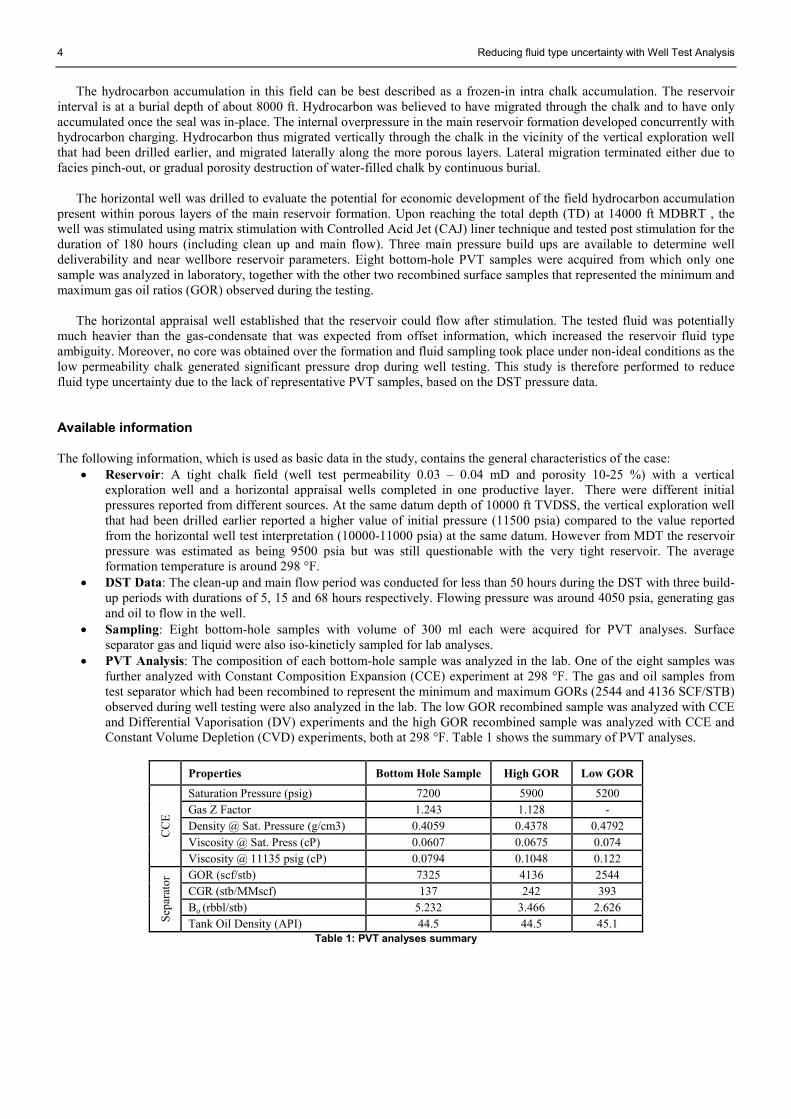
• PVT Analysis: The composition of each bottom-hole sample was analyzed in the lab. One of the eight samples was
further analyzed with Constant Composition Expansion (CCE) experiment at 298 °F. The gas and oil samples from
test separator which had been recombined to represent the minimum and maximum GORs (2544 and 4136 SCF/STB)
observed during well testing were also analyzed in the lab. The low GOR recombined sample was analyzed with CCE
and Differential Vaporisation (DV) experiments and the high GOR recombined sample was analyzed with CCE and
Constant Volume Depletion (CVD) experiments, both at 298 °F. Table 1 shows the summary of PVT analyses.
Properties Bottom Hole Sample High GOR Low GOR
CC
E
Saturation Pressure (psig) 7200 5900 5200
Gas Z Factor 1.243 1.128 -
Density @ Sat. Pressure (g/cm3) 0.4059 0.4378 0.4792
Viscosity @ Sat. Press (cP) 0.0607 0.0675 0.074
Viscosity @ 11135 psig (cP) 0.0794 0.1048 0.122
Sep
arat
or GOR (scf/stb) 7325 4136 2544
CGR (stb/MMscf) 137 242 393
Bo (rbbl/stb) 5.232 3.466 2.626
Tank Oil Density (API) 44.5 44.5 45.1
Table 1: PVT analyses summary

Reducing fluid type uncertainty with Well Test Analysis 5
Methodology and data analyses
PVT modelling
Fluid PVT model is very important for fluid type determination. The fluid properties from PVT modelling would be used later
in this study for the conversion of multiphase flow-rate to single phase flow-rate in Interpret 2010 (paradigm). This is because
TLSD (Total Least Square Deconvolution) which is used for the pressure-rate deconvolution only takes single phase flow-rate
as input. The PVT model would also be used for the 2-phase pseudo-pressure calculations.
Table 1 shows PVT data from three different fluid samples (bottom-hole, low GOR recombined and high GOR
recombined) that are available for the fluid type analysis. All the values recorded and reported during the field and lab test
were assumed to be valid. Prior to rejection of any information that presents an apparent inconsistency in the reported data; the
origin of its inconsistency was carefully analyzed. The compositional analysis of each sample was imported into PVTi
(Schlumberger) and the resulting phase envelope of each sample is shown in Figure 3. From the phase envelope, it can be seen
that at the reservoir conditions, the fluid type of bottom-hole sample falls within the gas condensate region but both fluid types
of the surface recombined samples fall within the volatile oil region. However from the laboratory PVT analysis, it was
reported that both bottom-hole and high GOR recombined samples existed in gas phase at reservoir conditions whereas only
the Low GOR recombined sample existed in volatile oil at the reservoir conditions. Therefore there is an inconsistency
between the compositional and PVT analyses for the high GOR recombined sample. Due to this inconsistency, the PVT data
could not be modelled in PVTi and would not be used further in this study.
Figure 3: Phase envelope for each reservoir fluid sample
In modelling the PVT properties of the reservoir fluid samples, the corrected Peng-Robinson (PR) equation of state (EOS)
with 3 parameters was used; together with Lorentz-Bray-Clark correlation for viscosity modelling. The PVT model for
bottom-hole sample was validated against CCE, and low GOR recombined sample was validated against CCE and DV
experiments. Regression was performed on molecular weight (MW), critical pressure (Pc) and critical temperature (Tc) of the
C7+ fraction pseudo-components; and binary interaction coefficients between light and heavy components. Figure 4 and 5
compare the observed and simulated CCE experiment for both bottom-hole and low GOR samples, respectively. Good
matches were achieved with C7+ components for both fluid samples with match error for each fluid property of less than 10%
except liquid saturation was difficult to model. Emphasizing the regression on the liquid saturation would compromise the
other PVT properties that would results in unrepresentative two-phase pseudo-pressure calculations.
Figure 4: Bottom-hole sample comparison of EOS model with CCE experiment

6 Reducing fluid type uncertainty with Well Test Analysis
Figure 5: Low GOR recombined sample comparison of EOS model with CCE experiment
Both PVT models from bottom-hole and low GOR recombined samples would be used separately from this point onward
to create two possible fluid types of gas condensate and volatile oil cases respectively. These fluids were analyzed independent
from each other.
Well Test Analysis
Data preparations
Deconvolution was used in the interpretation of the well test data, as the basis for pressure transient analysis. The pressure
and rate data (Figure 6) need to be properly prepared before applying deconvolution. Interpret 2010 and its functions were
used for data preparation. The start of test time was selected to be the time when the well flow-line was connected to the acid
injection line. The acid injection rates during well stimulation were retrieved from events sequence and synchronized with the
pressure data to accurately estimate the initial reservoir pressure, and a correct derivation of pressure derivatives. For
simplification purposes, the 15% HCl acid used during the stimulation was assumed to have similar properties as water. The
entire rate history was then simplified by reducing the number of flow periods (FP) by merging flow periods that have about
the same rate into one long flow period. There were initially 605 flow periods which later reduced to 76. Each flow period start
and end times were also synchronized with the pressure data to have correct pressure build ups and drawdowns. By using the
‘winnow’ function in Interpret 2010, the number of data points was also reduced before importing the pressure and rate data
into TLSD due to the limitation of data points. The reduction of data points also helped in enhancing the calculation speed. For
the gas condensate case, the pressure data was linearized into normalized single-phase pseudo-pressure (Eq.1) with the gas
condensate PVT properties from its PVT model. Figure 7 shows the rate validation where all of the three main build ups have
the same derivative stabilization. These build up would later be used for the wellbore skin effect study.
Figure 6: Pressure and rate data history from DST Figure 7: Rate validation of pressure build ups from DST

Reducing fluid type uncertainty with Well Test Analysis 7
Deconvolution – initial reservoir pressure
Deconvolution is a new tool that processes pressure and rate data to obtain more pressure data for well test interpretation. It
transforms variable-rate pressure data into a constant-rate initial drawdown with duration equal to the total duration of the test,
and yields directly the corresponding pressure derivative, normalized to a unit rate (Gringarten 2006, 2010). Deconvolution
removes the effects of rate variation from the pressure data measured during a well test sequence, thus the derivative is free
from errors introduced by incomplete or truncated rate history and distortions caused by pressure-derivative calculation
algorithms. As this process extracts more data available for interpretation than in the original data sets, it reveals underlying
characteristic system behaviour that has been dominating throughout the test, and is not governed only by a specific flow
period during the test (Levitan et al. 2004; Gringarten 2010).
Deconvolved pressure response is very sensitive to the value of initial reservoir pressure if the flow period being
deconvolved is infinite acting (Gringarten 2010) thus making it as a very crucial parameter in deconvolution. The initial
reservoir pressure entered by user affects the deconvolved pressure response at late time (Levitan et al. 2004). As there was
inconsistency in the reported initial reservoir pressure of this field between the vertical well, horizontal well and MDT
pressure, deconvolution was applied to correctly estimate the initial reservoir pressure by trial and error method. There are at
least two infinite acting build ups available from the DST pressure data to meet this purpose. The correct Pi must yield the
same deconvolved derivative (Levitan et al. 2004). For the gas condensate case, pressure data was converted to normalised
pseudo-pressure in order to approximate a linear system before applying deconvolution. To make Pi estimation more accurate,
the acidizing injection rates were included in deconvolving the pressure-rate data. Several initial pressures have been tested
and the deconvolved pressures of different build ups were compared with the longest build up pressure derivative. Figure 8
shows an initial pressure of 10620 psia yields almost identical deconvolved derivative for several flow periods for both volatile
and gas condensate cases. The deconvolved derivatives were also validated against the actual pressure history. Figures 9 and
10 show good matches were obtained between deconvolved derivatives and actual pressure data with maximum errors of less
than 10% in the drawdowns (Gringarten 2010).
Figure 8: Initial pressure determination for both gas condensate and volatile oil cases
Figure 9: Entire pressure match for gas condensate Figure 10: Entire pressure match for volatile oil
0.1
1
10
100
1000
0.0001 0.001 0.01 0.1 1 10 100 1000
De
con
vo
lve
d D
eri
va
tive
Elapsed Time (hrs)
Condensate Gas Pi Determination
FP 76
#(1-76)[76]{2.11292E+07}10620.00
#(1-76)[62]{5.37733E+07}10620.00
#(1-76)[62,66,76]{2.94528E+09}10620.00
#(1-76)[48-76]{4.16129E+09}10620.00
0.001
0.01
0.1
1
10
0.001 0.01 0.1 1 10 100 1000
De
con
vo
lve
d D
eri
va
tive
Elapsed Time (hrs)
Volatile Oil Pi Determination
FP 76
#(1-76)[76]{1.49772E+07}10620.00
#(1-76)[62]{3.65797E+07}10620.00
#(1-76)[62,66,76]{2.08782E+09}10620.00
#(1-76)[48-76]{2.88517E+09}10620.00
#(1-76)[1-76]{2.23112E+09}10620.00
8 Reducing fluid type uncertainty with Well Test Analysis
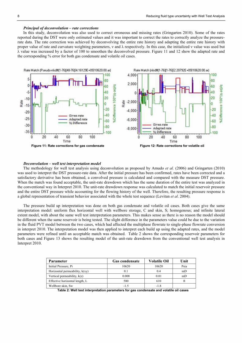
Principal of deconvolution – rate corrections
In this study, deconvolution was also used to correct erroneous and missing rates (Gringarten 2010). Some of the rates
reported during the DST were only estimated values and it was important to correct the rates to correctly analyze the pressure-
rate data. The rate correction was achieved by deconvolving the entire rate history and adapting the entire rate history with
proper value of rate and curvature weighting parameters, ν and λ respectively. In this case, the initialized ν value was used but
λ value was increased by a factor of 100 to smoothen the deconvolved pressure. Figure 11 and 12 show the adapted rate and
the corresponding % error for both gas condensate and volatile oil cases.
Figure 11: Rate corrections for gas condensate Figure 12: Rate corrections for volatile oil
Deconvolution – well test interpretation model
The methodology for well test analysis using deconvolution as proposed by Amudo et al. (2006) and Gringarten (2010)
was used to interpret the DST pressure-rate data. After the initial pressure has been confirmed, rates have been corrected and a
satisfactory derivative has been obtained, a convolved pressure is calculated and compared with the measure DST pressure.
When the match was found acceptable, the unit-rate drawdown which has the same duration of the entire test was analyzed in
the conventional way in Interpret 2010. The unit-rate drawdown response was calculated to match the initial reservoir pressure
and the entire DST pressure while accounting for the flowing history of the well. Therefore, the resulting pressure response is
a global representation of transient behavior associated with the whole test sequence (Levitan et al. 2004).
The pressure build up interpretation was done on both gas condensate and volatile oil cases. Both cases give the same
interpretation model: uniform flux horizontal well with wellbore storage, C and skin, S; homogenous; and infinite lateral
extent model, with about the same well test interpretation parameters. This makes sense as there is no reason the model should
be different when the same reservoir is being tested. The slight difference in the parameters value could be due to the variation
in the fluid PVT model between the two cases, which had affected the multiphase flowrate to single-phase flowrate conversion
in interpret 2010. The interpretation model was then applied to interpret each build up using the adapted rates, and the model
parameters were refined until an acceptable match was obtained. Table 2 shows the corresponding reservoir parameters for
both cases and Figure 13 shows the resulting model of the unit-rate drawdown from the conventional well test analysis in
Interpret 2010.
Parameter Gas condensate Volatile Oil Unit
Initial Pressure, Pi 10620 10620 Psia
Horizontal permeability, k(xy) 0.1 0.4 mD
Vertical permeability, k(z) 0.008 0.01 mD
Effective horizontal length, L 580 610 ft
Wellbore skin, Sw -1.5 -1.8
Table 2: Well test interpretation parameters for gas condensate and volatile oil cases

Reducing fluid type uncertainty with Well Test Analysis 9
Figure 13: Interpretation model for unit pressure drawdown for gas condensate case
2-phase pseudo-pressure analysis
The wellbore skin effect of gas condensate case was analyzed with two-phase pseudo-pressure (Eq. 3) due to the
development of region with different liquid saturations in the reservoir. For the case of volatile oil, the two-phase pseudo-
pressure is transformed to:
������ = ����!&���
�
� ��+ ��
� ��� �5�
where !& is the dissolve oil/gas ratio. The two-phase pseudo-pressure integral considers all the effects of two-phase fluid flow
and transforms it into a single fluid equivalent flow. This transformation accounts for the pressure dependent fluid properties
and relative permeability. There is no direct relationship between relative permeability ��� and �� with pressure but it can be
determined indirectly if a pressure-saturation relationship is defined for reservoir flowing conditions. Therefore the accuracy
of the calculation is very much dependent on the fluid PVT modelling.
There were different methods proposed to calculate two-phase pseudo-pressure. For the purpose of this study, the method
that was detailed by Bozorgzadeh (2006) in her PhD thesis is used. The correct radial flow stabilization which represents the
reservoir absolute permeability can be achieved when the GOR at the well stream saturation pressure Pbank is used to calculate
krg/kro (Bozorgzadeh and Gringarten, 2006). Pbank could be estimated from the single-phase pseudo-pressure derivative log-log
plot for gas condensate and rate-normalized pressure log-log plot for volatile oil. The fluid PVT properties required for
calculation were obtained from the simulated CVD experiment for the gas condensate case and Differential Vaporization
experiment for the volatile oil case.
Figure 14 shows the gas condensate single and two-phase pseudo-pressure log-log plot for the third build up (FP 76) from
the DST pressure-rate data. It can be seen that the 2-phase pseudo-pressure stabilizes at the same level the single-phase pseudo
pressure derivative stabilizes. The stabilization takes place at the first stabilization of horizontal well behaviour since the bank
only exists at the first stabilization. The calculated two-phase pseudo-pressure was then analyzed using the conventional well
test analysis in Interpret 2010.

10 Reducing fluid type uncertainty with Well Test Analysis
Figure 14: Single and two-phase pseudo-pressure log-log plot for gas condensate for FP 76 (PBU 3)
Figure 15: Two-phase pseudo-pressure log-log plot for volatile oil for FP 76 (PBU 3)
For the case of volatile oil fluid, since the bubble point pressure is considerably low (5200 psia) compared to the flowing
pressure (around 4100 psia), the existence of multiphase-flow region near the wellbore did not last very long before the gas
bank condensed back to the liquid phase during the pressure build-up. From the pressure-rate history and log-log plot
illustrated in Figure 6 and 7, it can be seen that the pressure builds up very fast that it surpasses the bubble points in a very
short time. Figure 15 shows the resulting two-phase pseudo-pressure log-log plot that was calculated for FP 76 and it was
confirmed that the two-phase flow region only exist within the period where wellbore storage effect dominated. The same case
applied for the other two pressure build ups FP 62 & FP 66. Due to this behaviour, the wellbore skin effect of volatile oil case
was analyzed through the normal rate-normalized pressure, instead of two-phase pseudo-pressure. The conventional well test
analysis was performed using Interpret 2010. Figure 16 shows the matches of well test analysis for the last build up of volatile
oil case.
Figure 16: Well test analysis for FP 76 - PBU 3 (volatile oil case)

Reducing fluid type uncertainty with Well Test Analysis 11
Results and discussion
Figure 17 and 18 show the skin effect for gas condensate and volatile oil cases, respectively. For the gas condensate case, the
skin effect was analyzed using two-phase pseudo-pressure since the flowing pressure was below the dew point pressure. On
the other hand, the volatile oil skin effect was only analyzed using the rate-normalized pressure as the bubble point pressure
was considerably lower than the pressure build up data. Therefore the volatile oil case could be considered as single-phase
flow.
Both cases show a positive trend of wellbore skin effect as rate increases but with different values of turbulence factor and
rate-independent skin. The gas condensate case yields a significant positive turbulence factor of 0.18 Day/MMscf, and a rate-
independent skin value of -1.7, while the volatile oil case yields a considerably small turbulence factor of 0.0013 Day/STB
with a lower rate-independent skin value of -3.7. The difference in the mechanical skin values is difficult to justify since there
was not enough pressure build ups above and below the saturation pressure to confirm the actual value.
Figure 17: Wellbore skin vs. rate for gas condensate case Figure 18: Wellbore skin vs. rate for volatile oil case
From a turbulence factor perspective, both cases yield the expected skin trend that corresponds to each fluid type as
published in the literature; small value for volatile oil and a positive trend for gas condensate (Gringarten et al. 2011).
However, for a fair comparison on the turbulence factor between the two cases, the comparison should be made using the
similar turbulence factor unit. In this case, the gas flowrates were used for the comparison since wellbore skin effects are
plotted against surface flowrates and both cases originated from the same surface flowrates. The wellbore skin effects from
both cases were plotted against the gas flowrates as shown in Figure 19. From this plot it can be seen that the turbulence factor
of volatile oil of 0.55 Day/MMscf is actually higher than the gas condensate itself and both cases still show an overall
increasing trend of wellbore skin effect with rates.
Figure 19: Wellbore skin vs. rate for both gas condensate and volatile oil cases
It is also important to emphasize that the analysis of the wellbore skin effect highly depends on the PVT model uncertainty.
Although both cases show an overall positive trend in wellbore skin effect with rate, Figures 19 shows that either the first or
second data point does not consistently follow the overall positive slope, and the flowrates for the first two data point are very
close to each other. This inconsistency could be due to the random rate histories observed during the DST but this rate history-
dependent skin effect is normally shown in the case of lean gas (Gringarten et al. 2011). However the molecular composition
(C1 between 60-70%) of the fluid that was tested did not show any possibility that the fluid could be a lean gas.
S = 0.18 Q - 1.7
-1.5
-1
-0.5
3 3.5 4 4.5 5
We
llbo
re s
kin
eff
ect
Gas rate, Q (MMscf/D)
S = 0.0013 Q - 3.7
-3
-2
-1
0
1500 1600 1700 1800 1900 2000
We
llbo
re s
kin
eff
ect
Oil rate, Q (STB/D)
S = 0.18 Q - 1.7
S = 0.55 Q - 3.7
-2.5
-1.5
-0.5
3.5 4 4.5 5
Wel
lbore
sk
in e
ffec
t
Gas rate, Q (MMSCFD)
Gas Condensate case
Volatile Oil case

12 Reducing fluid type uncertainty with Well Test Analysis
Regarding PVT model uncertainty, there was no CVD experiment performed on the bottom-hole sample for the gas
condensate case. The required CVD data for two-phase pseudo-pressure calculation was simulated in PVTi based on
regression against CCE experiment. The lack of experimental data could increase the uncertainty in PVT modeling. On the
other hand, the interpretation of volatile oil case did not involve two-phase pseudo-pressure calculation although PVT model
was used to convert multiphase flowrate to single-phase flowrate in the early stage of this study. The PVT modeling of volatile
oil was also supported by Differential Vaporization experiment in addition to the CCE experiment that both cases have in
common.
Conclusion
The results were derived from the information that was available from non-representative fluid samples and DST pressure-rate
data from a horizontal well. Based on the behavior of the wellbore skin effect from both cases, the behavior of the skins is
likely to associate with gas condensate system as both cases show a positive skin trend with rates.
Recommendations
The obtained results were derived base on fluid sample that was taken under non-ideal conditions and the recombined surface
samples according to the observed GORs. The representativeness of the fluid sample is still questionable. The uncertainty in
fluid properties could be reduced by having more lab-tested data from the bottom-hole samples that had been acquired during
fluid sampling. If another appraisal well were to be drilled, it is recommended to run downhole fluid analyzer that currently
available in the market to have better idea of the fluid at reservoir conditions, and to reduce uncertainty associated with fluid
handling methods.
The quality of well test analysis could also be enhanced if the flowrates were properly reported. Some of the reported
flowrates were just estimated values when the fluid was not flowed into test separator during the DST. Although
deconvolution could be used to correct the estimated rates, the resulting difference between the adapted and reported rates was
very significant. This difference could also contribute to the uncertainty in well test analysis.
The results of wellbore skin effect trend were only based on the three build up points. The wellbore skin effect study could
have been more representative if more pressure build ups data were available, above and below the saturation pressure with
broader range of flow-rates.
For future work, it is also a good idea to incorporate the DST data from the vertical well if it could help to reduce the fluid
type uncertainty. The vertical well DST was not used in this study due to unknown well stimulation history during the DST
which might have affected the wellbore skin effect differently.

13 Reducing fluid type uncertainty with Well Test Analysis
Nomenclature B = formation volume factor
CCE = constant composition expansion
CVD = constant volume depletion
D = non-Darcy coefficient
DV = differential vaporization
k = permeability
MMscf/D = million standard cubic feet per day
m(p) = pseudo-pressure
p = pressure
pbank = well stream saturation point pressure
PBU = pressure build up
PVT = pressure-volume-temperature
Q = production rate
Rp = producing gas/ oil ratio
Rs = solution gas /oil ratio
Rv = dissolved oil/gas ratio
s =skin
S = saturation
STB/D = standard barrel per day
TLSD = total least square deconvolution
Z = real gas compressibility
L = distance
Subscripts a = absolute
b = bubble
d = dew
eff = effective
g = gas
i = initial
m = mechanical
o = oil
r = relative
ref = reference
t = total
w = wellbore
1φ = one phase
2φ = two-phase
Greek λ = curvature weighting parameter
µ= viscosity
ρ = density
υ = velocity
ν = rate weighting parameter
References
Al-Hussainy, R., Ramey, H. J. Jr., and Crawford, P.B.: “The Flow of Real Gases through Porous Media”, J. Pet.Tech. (May 1966) 624.
Amudo, C., Turner, J., Frewin, J., Kgogo, T.C. and Gringarten, A.C.: “Integration of Well-Test Deconvolution Analysis and Detailed
Reservoir Modelling in 3D-Seismic Data Interpretation: A Case Study,” paper SPE 1000250, presented at the 2006 SPE Europe/EAGE
Annual Conference and Exhibition held in Vienna, Austria, Jun. 12-15.
Bozorgzadeh, M.: “Characterisation and Determination of Gas Condensate Dynamics from Pressure Transient Data and Fluid PVT
Properties. PhD thesis” Centre for Petroleum Studies, Imperial College London (2006).
Cobenas, R. H. and Crotti, M.A.: "Volatile Oil. Determination of Reservoir Fluid Composition From a Non-Representative Fluid Sample,"
paper SPE 54005 presented at 1999 SPE Latin American and Caribbean Petroleum Engineering Conference held in Caracas, Venezuela,
Apr. 21-23.
Gringarten, A. C., Bozorgzadeh, M., Daungkaew, S. and Hashemi, A.: “Well Test Analysis in Lean Gas Condensate Reservoirs: Theory and
Practice”, paper SPE 100993 presented at the 2006 SPE Russian Oil and Gas Technical Conference and Exhibition held in Moscow,
Russia, Oct. 3–6.
Gringarten, A.C., Ogunrewo, O. and Uxukbayev, G.: “Assessment of Rate-Dependent Skin Factors in Gas Condensate and Volatile Oil
Wells,” paper SPE 143592, presented at 2011 SPE EUROPEC/EAGE Annual Conference and Exhibition held in Vienna, Austria, May
23-26
Gringarten, A.C.: “From Straight lines to Deconvolution: the Evolution of the State of the Art in Well Test Analysis,” paper SPE 102079,
presented at the 2006 SPE Annual Technical Conference and Exhibition, San Antonio, Texas USA, Sep. 24-27
Gringarten, A.C.: “Practical use of well test Deconvolution,” paper SPE 134534, presented at the 2010 SPE Annual Technical Conference
and Exhibition held in Florence, Italy, Sep. 20-22
Jones, J. R. and Raghavan R.: “Interpretation of Flowing Well Response in Gas-Condensate Wells,” SPEFE (Sep. 1988) 578-594.
Levitan, M.M., Crawford, G. and Hardwick, A.: “Practical Considerations for Pressure-Rate Deconvolution of Well Test Data,” paper SPE
90680, presented at the 2004 SPE Annual Technical Conference and Exhibition held in Houston, Texas, USA, Sep. 26-29
Mc Cain Jr., W.: “Reservoir-Fluid Property Correlations - State of the Art,” SPERE (May 1991) 266.
Moses, P.: “Engineering Application of Phase Behavior of Crude Oil and Condensate Systems,” JPT (July 1985) 715.
PVTi version 2010.1, Schlumberger
Raghavan, R.: “Practical considerations in the Analysis of Gas-Condensate Well Tests,” SPEREE 2 (1999) (3): 288-295.
Saleh, A.M. and Stewart, G.: “Interpretation of Gas-Condensate Well Tests with Field Examples,” paper SPE 24719 presented at the 1992
SPE Annual Technical Conference, Washington DC, Oct. 4-7.
Sanni, M., and Gringarten, A.C.: “Well Test Analysis in Volatile Oil Reservoirs,” paper SPE 116239, presented at 2008 SPE Annual
Technical Conference and Exhibition held in Denver, Co, USA, Sep. 21-24.
Shandrygin, A., Rudenko, D.: “Condensate Skin Evaluation of Gas-Condensate Wells by Pressure –Transient Analysis,” paper SPE 97027
presented at the 2005 SPE Annual Technical Conference and Exhibition, Dallas, Texas, U.S.A., Oct. 9-12.
Smith, R.V.: “Unsteady-State Gas Flow into Gas Wells,” Jour. Pet. Tech. (Nov. 1961) 1151.
Thompson, L.G. and Reynolds, A.C.: “Well Testing for Gas-Condensate Reservoirs,” paper SPE 25371 presented at the 1993 Asia Pacific
Oil and Gas Conference, Singapore, Feb. 8-10.

14 Reducing fluid type uncertainty with Well Test Analysis
Xu S., Lee W. J.: “Two-Phase Well Test Analysis of Gas Condensate Reservoirs,” paper SPE 56483 presented at the 1999 SPE Annual
Conference and Exhibition, Houston, Texas, Oct. 3-6.

Reducing fluid type uncertainty with Well Test Analysis 15
APPENDIX A
Critical Literature Review
MILESTONES IN GAS CONDENSATE & VOLATILE OIL STUDY
TABLE OF CONTENT
SPE
Paper n°°°°
Year Title Authors Contribution
JPT 1965 “Two Phase Flow of Volatile
Hydrocarbons”
V.J. Kniazeff
S.A. Naville
- First to numerically model radial gas
condensate well deliverability.
- First to describe three different zones
around the well.
13185 1984 “Interpretation of Results From
Well Testing Gas-Condensate
Reservoirs: Comparison of
Theory and Field Cases”
P. Behrenbruch
G. Kozma
First to discuss wellbore dynamics effect
in gas condensate wells.
14204 1985 “Interpretation of Flowing Well
Response in Gas Condensate
Wells”
J. R. Jones,
R. Raghavan
First to propose a methodology for
analysing well tests in gas condensate
wells.
62920 2000 “Well Test Analysis in Gas
Condensate Reservoir”
A.C. Gringarten
A. Al-Lamki
S. Daungkaew
R. Mott
T. M. Whittle
First to use 3-region composite model to
analyse gas condensate well tests
100993 2006 Well Test Analysis in Lean Gas
Condensate Reservoirs: Theory
and Practice”
A.C. Gringarten
M. Bozorgzadeh
S. Daungkaew
A. Hashemi
First to report the increasing, decreasing
or remaining constant of wellbore skin
factor at high rates
Developing methodology to obtain gas
end point relative permeability, base
capillary number and critical oil
saturation
116239 2008 “Well Test Analysis in Volatile
Oil Reservoirs”
M. Sanni,
A.C. Gringarten
Discuss typical well test behaviours in
volatile oil reservoirs below the bubble
point pressure.
JCPT 2009 “Two-Phase Flow in Volatile Oil
Reservoirs Using Two-Phase
Pseudo-Pressure Well Test
Method”
M. Sharifi,
M. Ahmadi
Describe two-phase pseudo-pressure
method for well test interpretation of
volatile oil reservoirs which includes
predicting true permeability and
mechanical skin with good accuracy.
134534-MS 2010 “Practical Use of Well-Test
Deconvolution”
A.C. Gringarten Variety of practical applications of
deconvolution is presented such as
correction of erroneous rates from
DST’s, initial reservoir pressure
determination, identification of recharge
from reservoir layers and
compartmentalization - features which
conventional well test analysis could not
provide
143592 2011 “Assessment of Rate-Dependent
Skin Factors in Gas Condensate
and Volatile Oil Wells”
A.C. Gringarten
O. Ogunrewo
G. Uxukbayev
First paper to describe relationship of
rate-dependent skin below saturation
pressure calculated with two-phase
pseudo-pressure are identical to the
corresponding values calculated above
dew point pressure with single-phase
pseudo-pressure for condensate oil, and
pressure above bubble point pressure in
volatile oil reservoirs.

16 Reducing fluid type uncertainty with Well Test Analysis
1. SPE 143592 (2011)
Assessment of Rate-Dependent Skin Factors in Gas Condensate and Volatile Oil
Authors: Gringarten, A.C., Ogunrewo, O., Uxukbayev, G.
Contribution to the understanding of wellbore skin effect in well test analysis:
First to show below saturation pressure in gas condensate reservoir, single-phase pseudo-pressure well test analysis does not
correctly estimate the wellbore skin effect whereas analyses with two-phase pseudo-pressure do. Same goes for volatile oil,
below bubble point pressure, well test analysis with normal pressure do not correctly estimate the wellbore skin effect, but 2-
phase pseudo-pressure well test analysis can be used instead.
Objective of the paper:
To investigate the combined impact of capillary number and non-Darcy flow on the wellbore skin in lean and rich gas-
condensate reservoirs , using single-phase and two-phase pseudo-pressures, and to compare non-Darcy coefficients and zero-
rate skin factors above and below the saturation point pressure. Volatile oil reservoir was also included in the study.
Methodology used:
Compositional reservoir model was simulated with three different fluid types together with capillary number and non-Darcy
effects to evaluate their impact on the skin evaluation. In order to study the impact of the rate sequence on wellbore skin,
pressures for different rate histories (random, increasing and decreasing rates), were generated and analyzed for each type of
fluid.
Conclusion reached:
Verified that well test analysis with 2-phase pseudo-pressure does correctly estimate the rate-independent wellbore skin effect
and the non-Darcy flow coefficient in gas condensate and volatile oil wells below the saturation point pressure. The rate
independent skin factor and the non-Darcy flow coefficient calculated with two-phase pseudo-pressure are identical to the
corresponding values calculated above the saturation point pressure with single-phase pseudo-pressure for gas condensate and
pressure for volatile oil.
Comments:
The results were verified and confirmed with actual data from lean and rich gas condensates as well as volatile oil reservoir.
2. SPE 116239 (2008)
Well Test Analysis in Volatile Oil Reservoirs
Authors: Sanni, M., Gringarten, A.C.
Contribution to the understanding of the volatile oil reservoirs:
Understanding the behavior of volatile oil reservoir when the bottomhole pressure falls below the bubble point pressure
followed up subsequent build up
Objective of the paper:
To indentify typical well test behaviors in volatile oil reservoirs above and below the bubble point pressure
Methodology used:
Compositional numerical simulation was used to verify the effect of capillary number on well test data
Conclusion reached:
Existence of two-zone radial composite behavior when the bottomhole pressure falls below the bubble point pressure
During the buildup, the gas created around the well bore during the preceding drawdown condenses into the oil and initial gas
saturation is created.
Reducing fluid type uncertainty with Well Test Analysis 17
3. SPE 116239 (2004)
Well Test Analysis of Horizontal well in Gas-Condensate Reservoirs
Authors: Hashemi, A., Gringarten, A.C
Contribution to the understanding of the horizontal well gas condensate reservoirs:
The first to detail the near wellbore effects in well tests of horizontal wells in as condensate reservoir below the dew point
Objective of the paper:
To establish an understanding of the near-wellbore well test behavior in horizontal wells in gas condensate reservoirs, with a
focus on the existence of different mobility zones due to condensate dropout
Methodology used:
3D Compositional model was used to develop derivative shapes to be expected from horizontal well test data and actual field
data that exhibit the same characteristics was analyzed. Compositional model was used to verify the results from conventional
well test analysis
Conclusion reached:
In horizontal well test, condensate deposition creates a composite well test behavior similar to what is obtained in vertical
wells, but superimposed on a horizontal well behavior
Comments:
Actual well test behaviors were consistent with behaviors predicted from compositional simulations.
Only the derivative stabilization corresponding to the reduced mobility zones due to condensate deposit could be identified on
the log-log plot at early times. Derivative stabilization due to capillary number effects could not be identified due to the
dominating wellbore storage effect.
Due to complex PVT behavior in gas-condensate systems, both analytical well test analysis and compositional simulation are
required to analyze well test in horizontal well.
4. SPE 62920 (2000)
Well Test Analysis in Gas Condensate Reservoir
Authors: Gringarten, A.C., Al-Lamki, A., Daungkaew, S., Mott, R., Whittle, T.M.
Contribution to the understanding of the gas condensate reservoirs:
First to use three-zone radial composite model to analyze gas condensate well test data
Objective of the paper:
To investigate the existence of increased mobility zone in the near vicinity of the wellbore in well test data
Methodology used:
Compositional numerical simulations to verify existence of different mobility zones (Capillary number effects)
Analyzing well test data from numerous gas condensate fields
Conclusion reached:
Negative impact of phase distribution in analyzing well test data
Verification of the existence of three mobility zones on well test data

18 Reducing fluid type uncertainty with Well Test Analysis
5. SPE 134534-MS (2010)
Practical Use of Well-Test Deconvolution
Authors: A.C. Gringarten
Contribution to the understanding of a deconvolution method in well testing:
Proved that deconvolution is as a powerful tool in well test analysis and showed examples where decovolution was used in
identification of boundaries, connectivities and multilayer behavior in a gas condensate
Objective of the paper:
To recommendations on how to perform deconvolution and how to verify deconvolution results
To illustrate various applications of deconvolution well test interpretation
Methodology used:
Deconvolution of well test data from a gas condensate reservoir is applied on individual DST build-ups, build-ups during
production phase, groups of build-ups and continuous multi-flow periods & final unit-rate pressure drawdown analysis.
Deconvolution of DST data in an oil well. Comparison of pressure histories calculated from the deconvolved derivatives, with
and without rate adaptation, with actual pressure history.
Conclusion reached:
Deconvolution increases the radius of investigation, which allows seeing boundaries and connectivities not visible in
individual flow periods
Deconvolution corrects erroneous rates and determines missing rates.
Deconvolution can be applied to pseudo-linear systems such as with gas and multiphase flow.

Reducing fluid type uncertainty with Well Test Analysis 19
APPENDIX B
Geology illustration of the field
Figure B 1: Hydrocarbon accumulation system in the field under study

20 Reducing fluid type uncertainty with Well Test Analysis
APPENDIX C The comparison of EOS model results and experimental data for both bottom-hole and low GOR recombined samples are
shown in below presented figures.
Figure C 1: Comparison of EOS predicted and observed values from CCE experiment for bottom-hole sample

Reducing fluid type uncertainty with Well Test Analysis 21
Figure C 2: Comparison of EOS predicted and observed values from CCE experiment for low GOR recombined sample

22 Reducing fluid type uncertainty with Well Test Analysis
Figure C 3: Comparison of EOS predicted and observed values from DV experiment for low GOR recombined sample

Reducing fluid type uncertainty with Well Test Analysis 23
APPENDIX D
Well test interpretation model
The well test interpretation model from unit-rate pressure drawdown for volatile oil is shown below:
Figure D 1: Interpretation model from unit-rate drawdown for volatile oil case

24 Reducing fluid type uncertainty with Well Test Analysis
APPENDIX E
Well test interpretation for volatile oil case
Below are the pressure matched for volatile oil case, analyzed with normal pressure for the first two build up data:
Figure E 1: Well test interpretation for PBU 1 (volatile oil case)
Figure E 2: Well test interpretation for PBU 2 (volatile oil case)

Reducing fluid type uncertainty with Well Test Analysis 25
APPENDIX F Well test interpretation for gas condensate case
Below are the pressure matched for gas condensate case, analyzed with 2-phase pseudo-pressure:
Figure F 1: Well test interpretation for PBU 1 (gas condensate case)

26 Reducing fluid type uncertainty with Well Test Analysis
Figure F 2: Well test interpretation for PBU 2 (gas condensate case)
Figure F 3: Well test interpretation for PBU 3 (gas condensate case)
Top Related