


Languages
Pages
Legal


Impact of directional antennas on routing and neighbor discoveryin wireless ad-hoc networks
by
Gabriel ASTUDILLO BROCEL
THESIS PRESENTED TO ÉCOLE DE TECHNOLOGIE SUPÉRIEURE
IN PARTIAL FULFILLMENT FOR THE DEGREE OF
DOCTOR OF PHILOSOPHY
Ph. D.
MONTREAL, SEPTEMBER 7, 2017
ÉCOLE DE TECHNOLOGIE SUPÉRIEUREUNIVERSITÉ DU QUÉBEC
Gabriel Astudillo, 2017

This Creative Commons license allows readers to download this work and share it with others as long as the
author is credited. The content of this work cannot be modified in any way or used commercially.
BOARD OF EXAMINERS
THIS THESIS HAS BEEN EVALUATED
BY THE FOLLOWING BOARD OF EXAMINERS
M. Michel Kadoch, Thesis Supervisor
Département de génie électrique à l’École de technologie supérieure
M. Suryn Witold, President of the Board of Examiners
Département de génie logiciel et des TI à l’École de technologie supérieure
M. Zbigniew Dziong, Member of the jury
Département de génie électrique à l’École de technologie supérieure
M. Rommel Torres, External Independent Examiner
Electronics and Computer Science Department at Universidad Tecnica Particular de Loja
THIS THESIS WAS PRESENTED AND DEFENDED
IN THE PRESENCE OF A BOARD OF EXAMINERS AND THE PUBLIC
ON AUGUST 8, 2017
AT ÉCOLE DE TECHNOLOGIE SUPÉRIEURE


ACKNOWLEDGEMENTS
First and foremost, I would like to thank God for giving me the opportunity and the strength
to undertake this research study and to persevere until its completion. My gratitude also goes
to my wife Johanna and my daughter Nathalia who have filled my life with love and supported
me during all these years. Simply said, I owe them all and any success in my life.
Then, I would like to express my deepest gratitude to my supervisor Prof. Michel Kadoch for
his continuous support, insightful guidance, and inspirational mentorship. Thank you for your
opportune advice and for always encouraging me during my PhD. study.
I would also like to thank Prof. Suryn Witold, Prof. Rommel Torres and Prof. Zbigniew
Dziong for being part of my jury’s committee, your advice was a key factor in the completion
of this work.
Last, but not least, I would like to thank my friends and family for their support and help during
the duration of my studies.

IMPACT DES ANTENNES DIRECTIONNELLES SUR LE ROUTAGE ET LADÉCOUVERTE DE VOISINS DANS LES RÉSEAUX AD HOC SANS FIL
Gabriel ASTUDILLO BROCEL
RÉSUMÉLes réseaux ad hoc sans fil sont réseaux de données qui sont déployés sans infrastructure fixe
ni de contrôleurs centraux tels que les points d’accès ou les stations de base. Dans ces réseaux,
les paquets de données sont transmis directement au nœud de destination s’ils se situent dans
la plage de transmission de l’émetteur ou envoyés par nœuds intermédiaires agissant comme
relais. Ce paradigme, où une infrastructure fixe n’est pas nécessaire, est tolérant aux change-
ments de topologie, et permet un déploiement rapide a été considéré comme une technologie
prometteuse qui convient à un grand nombre d’implémentations de réseau, telles que les ap-
pareils portatifs, les capteurs sans fil et les réseaux de reprise après sinistres.
Récemment, les antennes directionnelles intelligentes ont été identifiées comme une technolo-
gie robuste qui peut améliorer la performance des réseaux ad hoc sans fil en termes de cou-
verture, de connectivité et de capacité. Contrairement aux antennes omnidirectionnelles qui
rayonnent de l’énergie dans toutes les directions, les antennes directionnelles peuvent focaliser
l’énergie dans une direction spécifique, en étendant la plage de couverture pour la même puis-
sance irradiée. Les gammes plus longues offrent des chemins plus courts aux autres nœuds et
améliorent également la connectivité. De plus, les antennes directionnelles peuvent réduire le
nombre de collisions dans un schéma d’accès basé sur les contentions, car elles peuvent diriger
le lobe principal dans la direction souhaitée et définir tous les autres comme nuls, réduisant
ainsi les interférences co-canal et réduisant le niveau de bruit. Les connexions sont plus fi-
ables en raison de la stabilité accrue des liaisons et de la diversité spatiale. Des chemins plus
courts, ainsi que des chemins alternatifs, sont également disponibles en raison de l’utilisation
d’antennes directionnelles.
La plupart des recherches antérieures se sont focalisés sur l’adaptation des protocoles de con-
trôle d’accès au media et d’acheminement existants pour utiliser les communications direction-
nelles. Ce travail de recherche est authentique car il améliore le processus de découverte du
voisin parce que il permet de découvrir des nœuds dans le deuxième voisinage d’un nœud
donné, en utilisant une procédure gossip-based et il permettre de partage l’information de
position relative obtenue au cours de cette étape avec le protocole de routage. Nous avons
également développé un modèle pour évaluer l’énergie consommée par les nœuds lorsque des
antennes directionnelles intelligentes sont utilisées dans le réseau ad-hoc. Cette étude a démon-
tré qu’en adaptant l’ouverture du faisceau des antennes, les nœuds sont capables d’atteindre les
nœuds les plus éloignés et par conséquent, diminuer le nombre de sauts entre la source et la
destination. Ceci va amellueure ne soulement le performance du réseau, mais réduit également
l’énergie moyenne consommée par l’ensemble du réseau.
Mots clés: antennes intelligentes, routage, reseaux ad-hoc, découverte du voisin

IMPACT OF DIRECTIONAL ANTENNAS ON ROUTING AND NEIGHBORDISCOVERY IN WIRELESS AD-HOC NETWORKS
Gabriel ASTUDILLO BROCEL
ABSTRACT
Wireless ad-hoc networks are data networks that are deployed without a fixed infrastructure
nor central controllers such as access points or base stations. In these networks, data packets
are forwarded directly to the destination node if they are within the transmission range of the
sender or sent through a multi-hop path of intermediary nodes that act as relays. This paradigm
where a fixed infrastructure is not needed, is tolerant to topology changes and allows a fast
deployment have been considered as a promissory technology that is suitable for a large num-
ber of network implementations, such as mobile hand-held devices, wireless sensors, disaster
recovery networks, etc.
Recently, smart directional antennas have been identified as a robust technology that can boost
the performance of wireless ad-hoc networks in terms of coverage, connectivity, and capac-
ity. Contrary to omnidirectional antennas, which can radiate energy in all directions, direc-
tional antennas can focus the energy in a specific direction, extending the coverage range for
the same power level. Longer ranges provide shorter paths to destination nodes and also im-
prove connectivity. Moreover, directional antennas can reduce the number of collisions in a
contention-based access scheme as they can steer the main lobe in the desired direction and set
nulls in all the others, thereby they minimize the co-channel interference and reduce the noise
level. Connections are more reliable due to the increased link stability and spatial diversity.
Shorter paths, as well as alternative paths, are also available as a consequence of the use of
directional antennas. All these features combined results in a higher network capacity.
Most of the previous research has focused on adapting the existing medium access control and
routing protocols to utilize directional communications. This research work is novel because
it improves the neighbor discovery process as it allows to discover nodes in the second neigh-
borhood of a given node using a gossip based procedure and by sharing the relative position
information obtained during this stage with the routing protocol with the aim of reducing the
number of hops between source and destination. We have also developed a model to evalu-
ate the energy consumed by the nodes when smart directional antennas are used in the ad-hoc
network. This study has demonstrated that by adapting the beamwidth of the antennas nodes
are able to reach furthest nodes and consequently, reduce the number of hops between source
and destination. This fact not only reduces the end-to-end delay and improves the network
throughput but also reduces the average energy consumed by the whole network.
Keywords: ad-hoc networks, routing, neighbor discovery, energy models, directional anten-
nas


TABLE OF CONTENTS
Page
CHAPTER 1 INTRODUCTION . . . . . . . . . . . . . . . . . . . . . . . . . . . . . . . . . . . . . . . . . . . . . . . . . . . . . . . . . . . . 1
1.1 Problem Statement . . . . . . . . . . . . . . . . . . . . . . . . . . . . . . . . . . . . . . . . . . . . . . . . . . . . . . . . . . . . . . . . . . . . . . . 2
1.2 Objectives . . . . . . . . . . . . . . . . . . . . . . . . . . . . . . . . . . . . . . . . . . . . . . . . . . . . . . . . . . . . . . . . . . . . . . . . . . . . . . . . 3
1.3 Methodology . . . . . . . . . . . . . . . . . . . . . . . . . . . . . . . . . . . . . . . . . . . . . . . . . . . . . . . . . . . . . . . . . . . . . . . . . . . . . 4
1.4 Thesis Contributions . . . . . . . . . . . . . . . . . . . . . . . . . . . . . . . . . . . . . . . . . . . . . . . . . . . . . . . . . . . . . . . . . . . . . 5
1.5 Thesis Outline . . . . . . . . . . . . . . . . . . . . . . . . . . . . . . . . . . . . . . . . . . . . . . . . . . . . . . . . . . . . . . . . . . . . . . . . . . . . 6
CHAPTER 2 LITERATURE REVIEW AND BACKGROUND . . . . . . . . . . . . . . . . . . . . . . . . . . 9
2.1 Introduction . . . . . . . . . . . . . . . . . . . . . . . . . . . . . . . . . . . . . . . . . . . . . . . . . . . . . . . . . . . . . . . . . . . . . . . . . . . . . . . 9
2.2 Ad-hoc Networks Basics . . . . . . . . . . . . . . . . . . . . . . . . . . . . . . . . . . . . . . . . . . . . . . . . . . . . . . . . . . . . . . . . . 9
2.2.1 Applications of Ad-hoc Networks . . . . . . . . . . . . . . . . . . . . . . . . . . . . . . . . . . . . . . . . . . . 10
2.2.2 Design and Research Challenges . . . . . . . . . . . . . . . . . . . . . . . . . . . . . . . . . . . . . . . . . . . . . 14
2.2.3 Requirements . . . . . . . . . . . . . . . . . . . . . . . . . . . . . . . . . . . . . . . . . . . . . . . . . . . . . . . . . . . . . . . . . . 15
2.3 Smart antennas technologies . . . . . . . . . . . . . . . . . . . . . . . . . . . . . . . . . . . . . . . . . . . . . . . . . . . . . . . . . . . . 17
2.3.1 Introduction . . . . . . . . . . . . . . . . . . . . . . . . . . . . . . . . . . . . . . . . . . . . . . . . . . . . . . . . . . . . . . . . . . . 17
2.3.2 Benefits of Smart Antenna Technologies . . . . . . . . . . . . . . . . . . . . . . . . . . . . . . . . . . . . 17
2.3.3 Foundation of smart antenna technology . . . . . . . . . . . . . . . . . . . . . . . . . . . . . . . . . . . . 19
2.4 Literature Review . . . . . . . . . . . . . . . . . . . . . . . . . . . . . . . . . . . . . . . . . . . . . . . . . . . . . . . . . . . . . . . . . . . . . . . 25
2.4.1 Modeling ad-hoc networks . . . . . . . . . . . . . . . . . . . . . . . . . . . . . . . . . . . . . . . . . . . . . . . . . . . 25
2.4.2 Neighborhood Discovery . . . . . . . . . . . . . . . . . . . . . . . . . . . . . . . . . . . . . . . . . . . . . . . . . . . . . 27
2.4.3 Routing Algorithms . . . . . . . . . . . . . . . . . . . . . . . . . . . . . . . . . . . . . . . . . . . . . . . . . . . . . . . . . . . 30
2.4.4 Energy Models . . . . . . . . . . . . . . . . . . . . . . . . . . . . . . . . . . . . . . . . . . . . . . . . . . . . . . . . . . . . . . . . 32
CHAPTER 3 MODELING DIRECTIONALITY IN WIRELESS AD-HOC
NETWORKS . . . . . . . . . . . . . . . . . . . . . . . . . . . . . . . . . . . . . . . . . . . . . . . . . . . . . . . . . . . . . . . . . 35
3.1 Introduction . . . . . . . . . . . . . . . . . . . . . . . . . . . . . . . . . . . . . . . . . . . . . . . . . . . . . . . . . . . . . . . . . . . . . . . . . . . . . . 35
3.2 Graph theory and Ad-hoc Networks . . . . . . . . . . . . . . . . . . . . . . . . . . . . . . . . . . . . . . . . . . . . . . . . . . . 36
3.3 System Model . . . . . . . . . . . . . . . . . . . . . . . . . . . . . . . . . . . . . . . . . . . . . . . . . . . . . . . . . . . . . . . . . . . . . . . . . . . 36
3.3.1 Node Distribution Model . . . . . . . . . . . . . . . . . . . . . . . . . . . . . . . . . . . . . . . . . . . . . . . . . . . . . 37
3.3.2 Network Topology . . . . . . . . . . . . . . . . . . . . . . . . . . . . . . . . . . . . . . . . . . . . . . . . . . . . . . . . . . . . 37
3.3.3 Antenna model . . . . . . . . . . . . . . . . . . . . . . . . . . . . . . . . . . . . . . . . . . . . . . . . . . . . . . . . . . . . . . . . 37
3.3.4 Wireless Channel Model . . . . . . . . . . . . . . . . . . . . . . . . . . . . . . . . . . . . . . . . . . . . . . . . . . . . . . 39
3.4 Simulation Setup . . . . . . . . . . . . . . . . . . . . . . . . . . . . . . . . . . . . . . . . . . . . . . . . . . . . . . . . . . . . . . . . . . . . . . . . 42
3.5 Analysis of Results . . . . . . . . . . . . . . . . . . . . . . . . . . . . . . . . . . . . . . . . . . . . . . . . . . . . . . . . . . . . . . . . . . . . . . 44
3.5.1 Link Probability . . . . . . . . . . . . . . . . . . . . . . . . . . . . . . . . . . . . . . . . . . . . . . . . . . . . . . . . . . . . . . . 44
3.5.2 Hop count . . . . . . . . . . . . . . . . . . . . . . . . . . . . . . . . . . . . . . . . . . . . . . . . . . . . . . . . . . . . . . . . . . . . . 46
CHAPTER 4 NEIGHBOR DISCOVERY AND ROUTING SCHEMES FOR
AD-HOC NETWORKS . . . . . . . . . . . . . . . . . . . . . . . . . . . . . . . . . . . . . . . . . . . . . . . . . . . . . 51
4.1 Introduction . . . . . . . . . . . . . . . . . . . . . . . . . . . . . . . . . . . . . . . . . . . . . . . . . . . . . . . . . . . . . . . . . . . . . . . . . . . . . . 51
XII
4.2 Overview . . . . . . . . . . . . . . . . . . . . . . . . . . . . . . . . . . . . . . . . . . . . . . . . . . . . . . . . . . . . . . . . . . . . . . . . . . . . . . . . 52
4.2.1 Neighbor Discovery . . . . . . . . . . . . . . . . . . . . . . . . . . . . . . . . . . . . . . . . . . . . . . . . . . . . . . . . . . . 52
4.2.2 Routing Algorithms . . . . . . . . . . . . . . . . . . . . . . . . . . . . . . . . . . . . . . . . . . . . . . . . . . . . . . . . . . . 54
4.3 System Model . . . . . . . . . . . . . . . . . . . . . . . . . . . . . . . . . . . . . . . . . . . . . . . . . . . . . . . . . . . . . . . . . . . . . . . . . . . 55
4.3.1 Antenna Model . . . . . . . . . . . . . . . . . . . . . . . . . . . . . . . . . . . . . . . . . . . . . . . . . . . . . . . . . . . . . . . . 55
4.3.2 Beamforming . . . . . . . . . . . . . . . . . . . . . . . . . . . . . . . . . . . . . . . . . . . . . . . . . . . . . . . . . . . . . . . . . . 57
4.4 Proposed Solution . . . . . . . . . . . . . . . . . . . . . . . . . . . . . . . . . . . . . . . . . . . . . . . . . . . . . . . . . . . . . . . . . . . . . . . 59
4.4.1 Neighbor discovery . . . . . . . . . . . . . . . . . . . . . . . . . . . . . . . . . . . . . . . . . . . . . . . . . . . . . . . . . . . 60
4.4.2 Directional Routing . . . . . . . . . . . . . . . . . . . . . . . . . . . . . . . . . . . . . . . . . . . . . . . . . . . . . . . . . . . 62
4.4.3 Route Discovery . . . . . . . . . . . . . . . . . . . . . . . . . . . . . . . . . . . . . . . . . . . . . . . . . . . . . . . . . . . . . . 64
4.4.4 Route Establishment . . . . . . . . . . . . . . . . . . . . . . . . . . . . . . . . . . . . . . . . . . . . . . . . . . . . . . . . . . 65
4.5 Simulation Setup . . . . . . . . . . . . . . . . . . . . . . . . . . . . . . . . . . . . . . . . . . . . . . . . . . . . . . . . . . . . . . . . . . . . . . . . 66
4.6 Results Analysis . . . . . . . . . . . . . . . . . . . . . . . . . . . . . . . . . . . . . . . . . . . . . . . . . . . . . . . . . . . . . . . . . . . . . . . . . 67
4.6.1 Average end to end delay . . . . . . . . . . . . . . . . . . . . . . . . . . . . . . . . . . . . . . . . . . . . . . . . . . . . . 67
4.6.2 Packet loss fraction . . . . . . . . . . . . . . . . . . . . . . . . . . . . . . . . . . . . . . . . . . . . . . . . . . . . . . . . . . . 68
4.6.3 Throughput . . . . . . . . . . . . . . . . . . . . . . . . . . . . . . . . . . . . . . . . . . . . . . . . . . . . . . . . . . . . . . . . . . . . 69
CHAPTER 5 ENERGY MODEL FOR DIRECTIONAL AD-HOC NETWORKS
. . . . . . . . . . . . . . . . . . . . . . . . . . . . . . . . . . . . . . . . . . . . . . . . . . . . . . . . . . . . . . . . . . . . . . . . . . . . . . . . . 71
5.1 Introduction . . . . . . . . . . . . . . . . . . . . . . . . . . . . . . . . . . . . . . . . . . . . . . . . . . . . . . . . . . . . . . . . . . . . . . . . . . . . . . 71
5.2 Proposed Model . . . . . . . . . . . . . . . . . . . . . . . . . . . . . . . . . . . . . . . . . . . . . . . . . . . . . . . . . . . . . . . . . . . . . . . . . 71
5.2.1 Node Distribution Model . . . . . . . . . . . . . . . . . . . . . . . . . . . . . . . . . . . . . . . . . . . . . . . . . . . . . 72
5.2.2 Network Topology . . . . . . . . . . . . . . . . . . . . . . . . . . . . . . . . . . . . . . . . . . . . . . . . . . . . . . . . . . . . 72
5.2.3 Antenna model . . . . . . . . . . . . . . . . . . . . . . . . . . . . . . . . . . . . . . . . . . . . . . . . . . . . . . . . . . . . . . . . 72
5.2.4 Wireless Channel Model . . . . . . . . . . . . . . . . . . . . . . . . . . . . . . . . . . . . . . . . . . . . . . . . . . . . . . 73
5.2.5 Graph Representation Matrix . . . . . . . . . . . . . . . . . . . . . . . . . . . . . . . . . . . . . . . . . . . . . . . . . 74
5.2.6 Routing scheme . . . . . . . . . . . . . . . . . . . . . . . . . . . . . . . . . . . . . . . . . . . . . . . . . . . . . . . . . . . . . . . 74
5.3 Energy Cost of Communication . . . . . . . . . . . . . . . . . . . . . . . . . . . . . . . . . . . . . . . . . . . . . . . . . . . . . . . . 76
5.3.1 Omnidirectional Energy Cost . . . . . . . . . . . . . . . . . . . . . . . . . . . . . . . . . . . . . . . . . . . . . . . . 77
5.3.2 Directional Energy Cost . . . . . . . . . . . . . . . . . . . . . . . . . . . . . . . . . . . . . . . . . . . . . . . . . . . . . . 79
5.4 Energy model for messages transmitted . . . . . . . . . . . . . . . . . . . . . . . . . . . . . . . . . . . . . . . . . . . . . . . 82
5.5 Simulation Setup . . . . . . . . . . . . . . . . . . . . . . . . . . . . . . . . . . . . . . . . . . . . . . . . . . . . . . . . . . . . . . . . . . . . . . . . 87
5.6 Results Analysis . . . . . . . . . . . . . . . . . . . . . . . . . . . . . . . . . . . . . . . . . . . . . . . . . . . . . . . . . . . . . . . . . . . . . . . . . 88
CONCLUSION AND RECOMMENDATIONS . . . . . . . . . . . . . . . . . . . . . . . . . . . . . . . . . . . . . . . . . . . . . . . 91
APPENDIX I LIST OF PUBLICATIONS . . . . . . . . . . . . . . . . . . . . . . . . . . . . . . . . . . . . . . . . . . . . . . . . . . 95
BIBLIOGRAPHY . . . . . . . . . . . . . . . . . . . . . . . . . . . . . . . . . . . . . . . . . . . . . . . . . . . . . . . . . . . . . . . . . . . . . . . . . . . . . . . 96
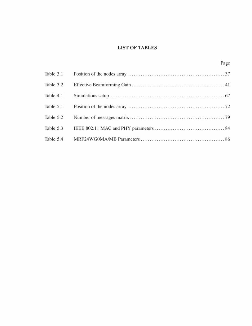
LIST OF TABLES
Page
Table 3.1 Position of the nodes array . . . . . . . . . . . . . . . . . . . . . . . . . . . . . . . . . . . . . . . . . . . . . . . . . . . . . . 37
Table 3.2 Effective Beamforming Gain . . . . . . . . . . . . . . . . . . . . . . . . . . . . . . . . . . . . . . . . . . . . . . . . . . . . 41
Table 4.1 Simulations setup . . . . . . . . . . . . . . . . . . . . . . . . . . . . . . . . . . . . . . . . . . . . . . . . . . . . . . . . . . . . . . . . 67
Table 5.1 Position of the nodes array . . . . . . . . . . . . . . . . . . . . . . . . . . . . . . . . . . . . . . . . . . . . . . . . . . . . . . 72
Table 5.2 Number of messages matrix . . . . . . . . . . . . . . . . . . . . . . . . . . . . . . . . . . . . . . . . . . . . . . . . . . . . . 79
Table 5.3 IEEE 802.11 MAC and PHY parameters . . . . . . . . . . . . . . . . . . . . . . . . . . . . . . . . . . . . . . . 84
Table 5.4 MRF24WG0MA/MB Parameters . . . . . . . . . . . . . . . . . . . . . . . . . . . . . . . . . . . . . . . . . . . . . . . 86


LIST OF FIGURES
Page
Figure 2.1 Mobile ad-hoc network topology . . . . . . . . . . . . . . . . . . . . . . . . . . . . . . . . . . . . . . . . . . . . . . 10
Figure 2.2 Community mesh network topology . . . . . . . . . . . . . . . . . . . . . . . . . . . . . . . . . . . . . . . . . . . 12
Figure 2.3 Opportunistic ad-hoc network . . . . . . . . . . . . . . . . . . . . . . . . . . . . . . . . . . . . . . . . . . . . . . . . . . 13
Figure 2.4 Device to Device Communications in 5G . . . . . . . . . . . . . . . . . . . . . . . . . . . . . . . . . . . . . 14
Figure 2.5 Smart directional antenna schematic . . . . . . . . . . . . . . . . . . . . . . . . . . . . . . . . . . . . . . . . . . . 20
Figure 2.6 Two infinitesimal dipoles . . . . . . . . . . . . . . . . . . . . . . . . . . . . . . . . . . . . . . . . . . . . . . . . . . . . . . . 21
Figure 2.7 Circular array of N elements . . . . . . . . . . . . . . . . . . . . . . . . . . . . . . . . . . . . . . . . . . . . . . . . . . . 22
Figure 2.8 AF elevation pattern for beamsteered circular array . . . . . . . . . . . . . . . . . . . . . . . . . . 23
Figure 2.9 An adaptive array structure . . . . . . . . . . . . . . . . . . . . . . . . . . . . . . . . . . . . . . . . . . . . . . . . . . . . . 24
Figure 2.10 Graph representation with omnidirectional antennas . . . . . . . . . . . . . . . . . . . . . . . . . 27
Figure 3.1 Antenna array installed in wireless nodes . . . . . . . . . . . . . . . . . . . . . . . . . . . . . . . . . . . . . 38
Figure 3.2 Different link models and resulting network topologies . . . . . . . . . . . . . . . . . . . . . . 42
Figure 3.3 Link probability comparisons . . . . . . . . . . . . . . . . . . . . . . . . . . . . . . . . . . . . . . . . . . . . . . . . . . 45
Figure 3.4 Nodes and links over a service area for different antenna
configurations . . . . . . . . . . . . . . . . . . . . . . . . . . . . . . . . . . . . . . . . . . . . . . . . . . . . . . . . . . . . . . . . . . . 47
Figure 3.5 Hopcount comparison: omnidirectional vs. directional model . . . . . . . . . . . . . . . 48
Figure 4.1 Antenna model for the switched beam array . . . . . . . . . . . . . . . . . . . . . . . . . . . . . . . . . . 56
Figure 4.2 Angle vs distance relationship . . . . . . . . . . . . . . . . . . . . . . . . . . . . . . . . . . . . . . . . . . . . . . . . . 57
Figure 4.3 Omnidirectional vs. directional range . . . . . . . . . . . . . . . . . . . . . . . . . . . . . . . . . . . . . . . . . 60
Figure 4.4 Antenna clockwise scan . . . . . . . . . . . . . . . . . . . . . . . . . . . . . . . . . . . . . . . . . . . . . . . . . . . . . . . . 61
Figure 4.5 Route discovery with omnidirectional antennas . . . . . . . . . . . . . . . . . . . . . . . . . . . . . . . 65
Figure 4.6 Route establishment with directional antennas . . . . . . . . . . . . . . . . . . . . . . . . . . . . . . . . 66
XVI
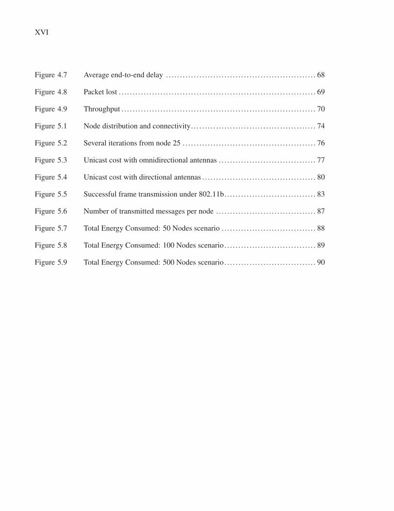
Figure 4.7 Average end-to-end delay . . . . . . . . . . . . . . . . . . . . . . . . . . . . . . . . . . . . . . . . . . . . . . . . . . . . . . 68
Figure 4.8 Packet lost . . . . . . . . . . . . . . . . . . . . . . . . . . . . . . . . . . . . . . . . . . . . . . . . . . . . . . . . . . . . . . . . . . . . . . . 69
Figure 4.9 Throughput . . . . . . . . . . . . . . . . . . . . . . . . . . . . . . . . . . . . . . . . . . . . . . . . . . . . . . . . . . . . . . . . . . . . . . 70
Figure 5.1 Node distribution and connectivity. . . . . . . . . . . . . . . . . . . . . . . . . . . . . . . . . . . . . . . . . . . . . 74
Figure 5.2 Several iterations from node 25 . . . . . . . . . . . . . . . . . . . . . . . . . . . . . . . . . . . . . . . . . . . . . . . . 76
Figure 5.3 Unicast cost with omnidirectional antennas . . . . . . . . . . . . . . . . . . . . . . . . . . . . . . . . . . . 77
Figure 5.4 Unicast cost with directional antennas . . . . . . . . . . . . . . . . . . . . . . . . . . . . . . . . . . . . . . . . . 80
Figure 5.5 Successful frame transmission under 802.11b. . . . . . . . . . . . . . . . . . . . . . . . . . . . . . . . . 83
Figure 5.6 Number of transmitted messages per node . . . . . . . . . . . . . . . . . . . . . . . . . . . . . . . . . . . . 87
Figure 5.7 Total Energy Consumed: 50 Nodes scenario . . . . . . . . . . . . . . . . . . . . . . . . . . . . . . . . . . 88
Figure 5.8 Total Energy Consumed: 100 Nodes scenario . . . . . . . . . . . . . . . . . . . . . . . . . . . . . . . . . 89
Figure 5.9 Total Energy Consumed: 500 Nodes scenario . . . . . . . . . . . . . . . . . . . . . . . . . . . . . . . . . 90

LIST OF ALGORITHMS
Page
Algorithm 3.1 Find Neighbors Function . . . . . . . . . . . . . . . . . . . . . . . . . . . . . . . . . . . . . . . . . . . . . . . . . . . 43
Algorithm 4.1 4-way handshaking with extended range . . . . . . . . . . . . . . . . . . . . . . . . . . . . . . . . . . 63


LIST OF ABREVIATIONS
AE Average Energy Matrix
ACK Acknowledge Message
AODV Ad-hoc On Demand Distance Vector
CTS Clear To Send Signal
CRC Cyclic Redundancy Check
CSMA/CA Carrier Sense Multiple Access / Collision Avoidance
CW Contention Window
DIFS Distributed Inter Frame Space
DSR Dynamic Source Routing
DO Directional-Omnidirectional
DD Directional-Directional
DSP Digital Signal Processor
DRX-AODV Directional with Extended Range AODV
FDMA Frequency Division Multiple Access
FSO Free Space Optical
GPS Global Positioning System
IEEE Institute of Electrical and Electronic Engineers
LAR Location Aided Routing
LEOD Location Enhancend on Demand Protocol

XX
MAC Medium Access Control
MANET Mobile Ad-hoc Network
MSE Minimun Square
NB Neighbor Discovery
N-BF Beam Forming
NS3 Network Simulator version 3
OD Omnidirectiona-Directional
PEER Progressive Energy-Efficient Routing
RREQ Route Request Packet
RREP Route Reply Packet
RTS Request To Send Signal
SIFS Short Inter Frame Space
SP Signal Processor
SIR Signal to Interference Ratio
SDMA Spatial Division Multiple Access
TDMA Time Division Multiple Access
TE Total Energy Matrix
TCP Transfer Control Protocol
TCP/IP Transfer Control / Internet Protocol
TBRPF Topology Dissemination Based on Reverse-path Forwarding

XXI
WSN Wireless Sensor Networks
WMA Wireless Multicast Advantage
WMN Wireless Mesh Networks


LISTE OF SYMBOLS AND UNITS OF MEASUREMENTS
Pr Power received
Pt Power transmitted
Gr Reception Antenna Gain
Gt Transmission Antenna Gain
PL Power Losses
Prmin Minimum power received
γ Threshold
PL(d0) Power Losses at reference distance d0
d0 Reference distance
Eθ Electric field
φ Electrical phase difference
θ Angle
wn Beam former weight n
δn Phase n
θ0 Angel of reference
wk,i weight vector
r0 Reference distance
ρ Node density
p(ri j) link probability between node i and j
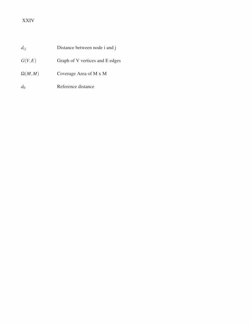
XXIV
di j Distance between node i and j
G(V,E) Graph of V vertices and E edges
Ω(M,M) Coverage Area of M x M
d0 Reference distance
CHAPTER 1
INTRODUCTION
From a general point of view a wireless ad-hoc network interconnects static or mobile nodes
with wireless links and if required it can implement gateway functions to other types of net-
works such as cellular, broadband access, the Internet and many others. The major character-
istic of this type of network is the wireless multi-hop architecture implemented in the network.
The self-configuring capacity, low upfront cost, and ease of deployment have drawn a lot of
attention from the international research community during the last decade. Despite these
advantages, wireless ad-hoc networks face several issues particularly when the size of the net-
work increases considerably (scalability issues) and when the velocity of the nodes increases
(mobility issues).
There has been a recent trend in wireless ad-hoc networks in order to increase the scalability,
efficient spectral reuse, and higher achievable bandwidth: the introduction of directionality in
the communication methods (e.g. smart directional antennas, sectored antennas and free-space-
optical transceivers). The improvements that can be achieved are promising and it becomes
interesting to investigate how directionality can be successfully implemented in wireless ad-
hoc networks. In this thesis, we analyze the improvement that can be achieved when smart
directional antennas are used in ad-hoc networks.
Although a lot of work has been done on this subject, most of the previous research has focused
on adapting existing MAC and routing protocols to utilize directional communications. To the
best of our knowledge, our work is novel because it improves the neighbor discovery process
as it allows to discover nodes in the second neighborhood of a given node using a gossip based
procedure and by sharing the relative position information obtained during this stage with the
routing protocol with the aim to reduce the number of hops between source and destination.
We have also developed a model to evaluate the energy consumed by the nodes when smart
directional antennas are used in the ad-hoc network. The goal of this thesis is to prove that by

2
adapting the beamwidth of the antennas to reach the farthest nodes and consequently, reducing
the number of hops between source and destination not only reduces the end-to-end delay
and improves the network throughput, but it also reduces the whole network’s average energy
consumed.
1.1 Problem Statement
In recent years, wireless ad-hoc networks have emerged as a promising technology for In-
ternet broadband access, community data networks, disaster recovery, vehicular and military
networks due to its ease of deployment and low up-front investment. Exploiting this advan-
tages requires new protocols and mechanisms at various communication layers to efficiently
control the directional antenna beam. With directional antennas many trivial mechanisms such
as neighborhood discovery and routing mechanisms become challenging. In this section we
will identify and describe these issues:
• Directional modeling of transmissions in ad-hoc networks: Due to the absence of com-
mercial solutions and the complexity of the ad-hoc scenarios, simulations have emerged as
a widely accepted method to evaluate the performance of ad-hoc networks. However, sim-
ulation models can not always provide a deep understanding of the relationship between
network performance and specific parameters. For this reason, many recent research ef-
forts have considered the use of mathematical models to better explain the aforementioned
relationships. Nevertheless, more of the previous work considered omnidirectional trans-
missions in the models and we have identified that there are very few models that consider
the directional transmission in the mathematical model of ad-hoc networks;
• Path length reduction with directional beams: When the number of nodes in the network
increases, the number of hops needed to reach distant nodes also increases. Besides, when
a packet arrives at a node it needs to be processed to determine the next hop, this procedure
increases the delay in the information delivery. Therefore each hop contributes to the de-
lay related to packet processing, route calculation, and propagation. As consequence, the
3
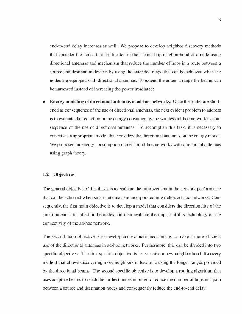
end-to-end delay increases as well. We propose to develop neighbor discovery methods
that consider the nodes that are located in the second-hop neighborhood of a node using
directional antennas and mechanism that reduce the number of hops in a route between a
source and destination devices by using the extended range that can be achieved when the
nodes are equipped with directional antennas. To extend the antenna range the beams can
be narrowed instead of increasing the power irradiated;
• Energy modeling of directional antennas in ad-hoc networks: Once the routes are short-
ened as consequence of the use of directional antennas, the next evident problem to address
is to evaluate the reduction in the energy consumed by the wireless ad-hoc network as con-
sequence of the use of directional antennas. To accomplish this task, it is necessary to
conceive an appropriate model that considers the directional antennas on the energy model.
We proposed an energy consumption model for ad-hoc networks with directional antennas
using graph theory.
1.2 Objectives
The general objective of this thesis is to evaluate the improvement in the network performance
that can be achieved when smart antennas are incorporated in wireless ad-hoc networks. Con-
sequently, the first main objective is to develop a model that considers the directionality of the
smart antennas installed in the nodes and then evaluate the impact of this technology on the
connectivity of the ad-hoc network.
The second main objective is to develop and evaluate mechanisms to make a more efficient
use of the directional antennas in ad-hoc networks. Furthermore, this can be divided into two
specific objectives. The first specific objective is to conceive a new neighborhood discovery
method that allows discovering more neighbors in less time using the longer ranges provided
by the directional beams. The second specific objective is to develop a routing algorithm that
uses adaptive beams to reach the farthest nodes in order to reduce the number of hops in a path
between a source and destination nodes and consequently reduce the end-to-end delay.
4
The third main objective is to develop a model for the energy consumption on ad-hoc networks
when the smart directional antennas are used on the nodes. Then, the model should be used to
determine the amount of energy that can be saved when the smart antenna technology is used
in ad-hoc networks.
1.3 Methodology
In this research, we study new ways of using smart directional antennas in ad-hoc networks.
Specifically, on the neighbor discovery mechanism and on the routing protocol. These prob-
lems are addressed in three stages.
In the first stage, we address the problem of modeling the impact of directional antennas on
the connectivity of ad-hoc networks. The model should consider the effect of directionality on
the link probability and analyze its consequences on the network connectivity. Thus, this stage
consist of two components: The link probability model, which should be expressed as a func-
tion of the antenna gains installed in the nodes, and the connectivity model that is determined
as a function of the average hop count in the wireless network.
We propose to model these problems using graph theory, since literature survey reveals that
mathematical model of ad-hoc networks is gaining considerable attention as alternative to sim-
ulation based models (Németh and Vattay (2003); Glauche et al. (2003)). In fact, graph theory
is a widely used tool to model many types of relations and processes in physical, social and
information systems. Emphasizing its application to real-world systems, the term network is
sometimes defined to mean a graph in which attributes are associated with the nodes and edges.
In the second stage, we develop two algorithms that attempt to take full advantage of the ca-
pabilities of smart antennas. The first algorithm aims at increasing the number of discovered
nodes by considering the nodes that are located in the second-hop neighborhood of a node
(gossip-based algorithm with directional antennas). The second algorithm seeks to reduce the
number of hops in a route between source and destination devices by using the extended range
that can be achieved when the nodes are equipped with directional antennas. To extend the
5
antenna range, we propose to narrow the antenna beam instead of increase the power irradi-
ated. This will reduce the energy consumption and reduce the number of retransmissions as a
consequence of the packet collisions.
The third stage attempts to evaluate the reduction in the energy consumed by the wireless
ad-hoc network as consequence of the implementation of the two algorithms proposed in the
second stage. To accomplish this task it is necessary to conceive an appropriate model that
considers the directional antennas on the energy model. Following the methodology used in the
first stage, a novel energy consumption model for ad-hoc networks with directional antennas
using Graph Theory is proposed.
The graph theoretical models are implemented using MATLAB version 2013A and the Graph
Theory (GT) Toolbox; the routing models are also implemented on MATLAB with the support
of the Network Analysis and Visualization toolbox.
1.4 Thesis Contributions
As result of the objectives presented in this thesis and following the proposed methodology,
this research work makes the following novel contributions:
• a directional link probability model that considers the antenna gains is used as a function to
weight the edges of a geometric random graph representation of a wireless ad-hoc network;
then, the connectivity of the network is evaluated in terms of the number of the hops in a
route (C-2);
• a novel neighbor discovery mechanism that uses a gossip-based mechanism to discover
nodes in the second neighborhood of a node, and uses the extended range of directional
antennas to reach farthest nodes(J-1);
• a routing algorithm that efficiently reduces the number of hops during the route discovery
using the information provided by the neighbor discovery algorithm also proposed in this
thesis (C-1 and J-1);

6
• an energy model that considers the directionality of the antennas in the function used to
weight the edges of a random graph and then, the energy consumed in the network is
evaluated and compared with traditional protocols (J-2).
1.5 Thesis Outline
The rest of this thesis is organized as follows: In Chapter 1, we present a background about
wireless ad-hoc networks, their primary applications, as well as the design and research chal-
lenges that this type of networks faces. We also introduce the smart directional antenna tech-
nology, its applications, and most used array types. We finish the first chapter with a detailed
description of the related work that has been done in the neighbor discovery, routing protocols
and energy models for ad-hoc networks.
In Chapter 2, we investigate the impact of smart antennas on the connectivity of wireless ad-
hoc networks by considering directional transmissions on the link probability model. We define
the system model and we also state the assumptions considered at this stage of the thesis. We
complete the chapter with an analysis of the results obtained.
Chapter 3 presents a gossip-based neighbor discovery algorithm that uses the information pro-
vided by directional antennas to discover neighbors in the second neighborhood of the node
using directional beams. Then, a routing algorithm that aims to reduce the number of hops
during the route construction using the information provided by the neighborhood discovery
algorithm is also proposed in this article. We conclude this chapter with a comprehensive com-
parison between the scheme proposed in this article and similar solutions previously developed.
In Chapter 4, we present an energy model that considers the directionality of smart antennas.
An extensive review of the models developed in this research topic introduces the chapter, then
the assumptions made in our model are described as is the model itself. We conclude this
chapter with a description of the simulations setup and an analysis of the obtained results.

7
Finally, we summarize this research work and present our conclusions and recommendations
based on the analysis of the obtained results. We also provide some insights about the future
directions that can be followed in this research line.


CHAPTER 2
LITERATURE REVIEW AND BACKGROUND
2.1 Introduction
In this chapter, we present the key concepts used in this thesis. The first section is dedicated
to introducing the basics concepts of ad-hoc networks. Subjects as applications, design and
research challenges, requirements and their impact on 5G communications are discussed in this
section. Then, the smart antennas technologies are described. The benefits offered by this type
of antennas, their fundamental concepts and possible impact in ad-hoc networks are presented
in this section. We finalize this chapter by reviewing the state of the art in the research areas of
routing protocols, neighbor discovery methods and energy consumption models of these type
of wireless networks.
2.2 Ad-hoc Networks Basics
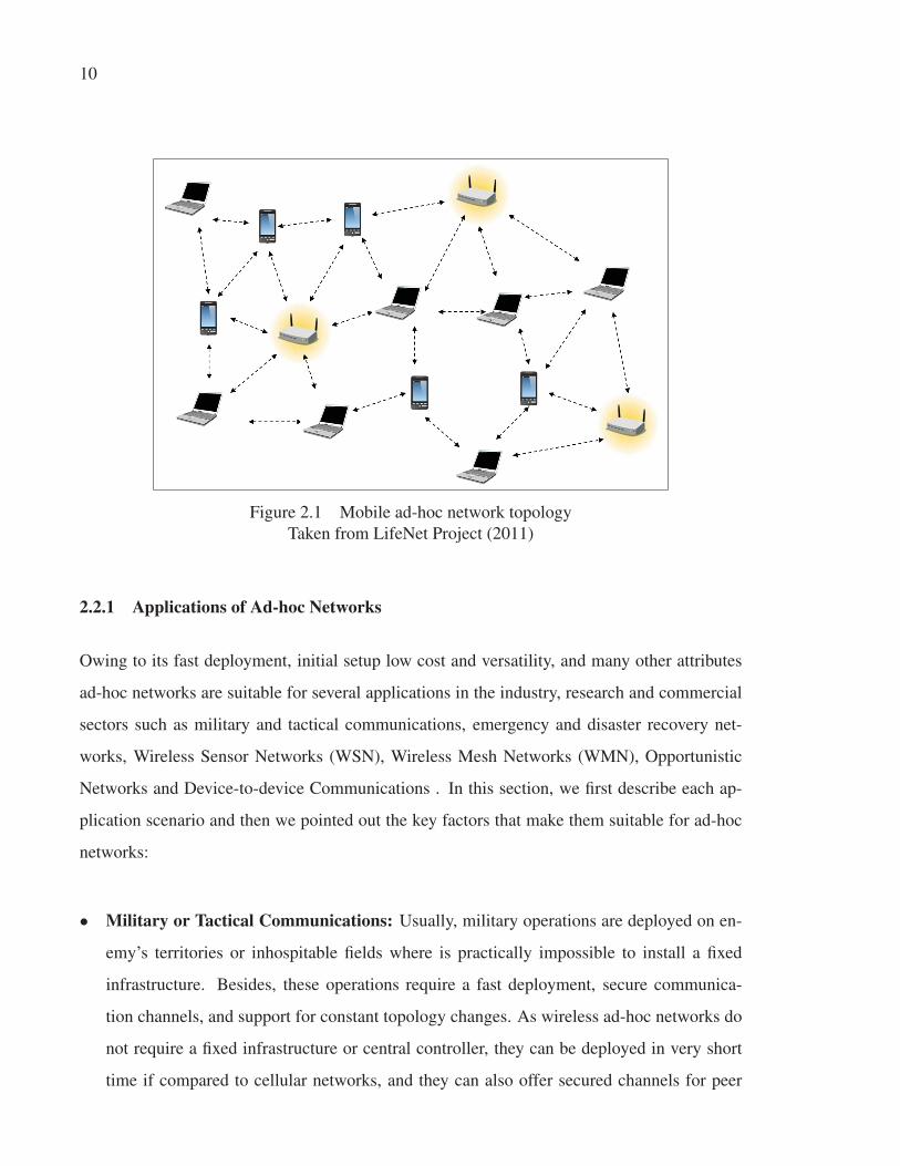
Wireless ad-hoc networks are data networks that are deployed without a fixed infrastructure or
central controllers such as access points or base stations as schematized in Figure 2.1. In these
networks, data packets are forwarded directly to the destination, if it is in the transmission range
of the sender, or indirectly, through a multi-hop path of intermediary nodes that act as relays.
This paradigm where a fixed infrastructure is not needed, is tolerant to topology changes and
allows a fast deployment, is suitable for a large number of network implementations, such as
mobile handheld devices, wireless sensors, disaster recovery networks, tactical networks and
many others.
The versatility, low initial setup cost and ease of deployment allowed several manufacturers to
enter into the ad-hoc networking field with different products and applications. Although they
bring many advantages, ad-hoc networks face several issues particularly when the size of the
network increases considerably, also know as scalability issues and when the velocity of the
nodes increases from now on, mobility issues.
10
Figure 2.1 Mobile ad-hoc network topology
Taken from LifeNet Project (2011)
2.2.1 Applications of Ad-hoc Networks
Owing to its fast deployment, initial setup low cost and versatility, and many other attributes
ad-hoc networks are suitable for several applications in the industry, research and commercial
sectors such as military and tactical communications, emergency and disaster recovery net-
works, Wireless Sensor Networks (WSN), Wireless Mesh Networks (WMN), Opportunistic
Networks and Device-to-device Communications . In this section, we first describe each ap-
plication scenario and then we pointed out the key factors that make them suitable for ad-hoc
networks:
• Military or Tactical Communications: Usually, military operations are deployed on en-
emy’s territories or inhospitable fields where is practically impossible to install a fixed
infrastructure. Besides, these operations require a fast deployment, secure communica-
tion channels, and support for constant topology changes. As wireless ad-hoc networks do
not require a fixed infrastructure or central controller, they can be deployed in very short
time if compared to cellular networks, and they can also offer secured channels for peer

11
to peer communications. For these reasons, ad-hoc networks are considered as one of the
most suitable solutions for military applications as well as tactical communications for civil
defense or firefighting corps;
• Emergency and Disaster Recovery Networks: Natural disasters such as earthquakes or
hurricanes can devastate extended populated zones and leave many people without telecom-
munications services. In this situations, it is critical to restore the communication services
as soon as possible as well as to support tactical communications between rescue services,
humanitarian organizations and government institutions. With ad-hoc networks, this ser-
vices can be reestablished in hours instead of weeks, which would be the case if using
wired or cellular networks. The multi-hop paradigm can also extend the coverage area as
well as overcome the line of sight (LOS) issue which can be a turning point in geographic
zones with a geographical singularity;
• Wireless Sensor Networks: Wireless Sensor Networks are a collection of sensors de-
ployed in a specific geographical area that is connected wirelessly. The nodes are usually
tiny devices that gather information about physical conditions around the sensors, then pro-
cess the data and transport it to one or more gateways that are connected to the Internet.
As the nodes are supposed to sense a parameter in a specific region, they usually do not
move, so mobility is not considered. Besides, these nodes are placed in areas which are dif-
ficult to access or where it is not possible to connect to the public electric grid, so they are
commonly battery powered. As batteries have a limited lifetime, it is important to develop
protocols that are energy efficient and consider power constraints in their designs. Finally,
the size of the network is usually larger than another type of ad-hoc networks;
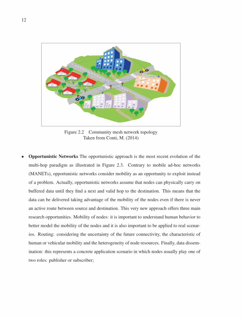
• Wireless Mesh Networks: Wireless mesh networks (WMNs) are intended to provide
broadband Internet access to mobile or fixed users as an alternative to cellular o wired
networks, as illustrated in Figure 2.2. There are several advantages of WMNs such as the
unnecessity of frequency reuse, the redundancy of the paths between the source and desti-
nation nodes, and higher bandwidths. Moreover, the use of unlicensed frequency bands and
the installation of routers on rooftops or posts reduce the cost of deployment and operation;
12
Figure 2.2 Community mesh network topology
Taken from Conti, M. (2014)
• Opportunistic Networks The opportunistic approach is the most recent evolution of the
multi-hop paradigm as illustrated in Figure 2.3. Contrary to mobile ad-hoc networks
(MANETs), opportunistic networks consider mobility as an opportunity to exploit instead
of a problem. Actually, opportunistic networks assume that nodes can physically carry on
buffered data until they find a next and valid hop to the destination. This means that the
data can be delivered taking advantage of the mobility of the nodes even if there is never
an active route between source and destination. This very new approach offers three main
research opportunities. Mobility of nodes: it is important to understand human behavior to
better model the mobility of the nodes and it is also important to be applied to real scenar-
ios. Routing: considering the uncertainty of the future connectivity, the characteristic of
human or vehicular mobility and the heterogeneity of node resources. Finally, data dissem-
ination: this represents a concrete application scenario in which nodes usually play one of
two roles: publisher or subscriber;

13
Figure 2.3 Opportunistic ad-hoc network
Taken from Conti, M. (2014)
• Ad-hoc applications in 5G: D2D communication The next paradigm in wireless commu-
nications widely known as fifth generation (5G), aims at providing the end users with ubiq-
uitous connectivity worldwide despite the technology used (cellular/wireless/FSO). While
the conventional cellular architecture consists of connections from base stations to user
equipment, 5G systems may rely upon a two-tier architecture consisting of a macro cell
tier for base station to device communication, and a second device tier for device to device
(D2D) communications. Such architectures are a hybrid of conventional cellular and ad
hoc networks. Thus, integration of MANET with cellular architectures solves the coverage
and connectivity problem providing a reliable ubiquitous connection (see Figure 2.4). The
future is promissory for ad-hoc communications but lessons have to be learned from the
past and real scenarios, as well as specific applications instead of general approaches, must
be considered in order to attract the interest of the industry and network operators.

14
Figure 2.4 Device to Device Communications in 5G
Taken from Conti, M. (2014)
2.2.2 Design and Research Challenges
In this section, we present the main challenges that face the scientific community and the
industry regarding of design and open research issues. Although during the past two decades a
lot of work has been done in this area there are still several issues that need to be addressed and
some others that have emerged as a consequence of the evolution of the wireless technology:
• Security Issues and Challenges: To have secure communications among mobile nodes
is a priority issue. During years security has been an active research theme. MANETs
present several new challenges for researchers and developers like open network architec-
ture, shared wireless medium and highly dynamic network topology. Nevertheless, the
existing security measures do not cover MANETs and it is necessary the implementation
of news security solutions. The routing protocols for wireless ad-hoc networks should be
able to solve all these issues efficiently;
• Bandwidth constraint: The broadcast condition is inherent to ad-hoc networks. There-
fore, the available bandwidth per wireless link depends on the number of nodes and the
traffic they handle. Thus, only a fraction of the total bandwidth is effectively available for

15
transmission and reception in every node. On the other hand, mobility of the nodes makes
established routes to broke thus route reparation procedures have to run, these procedures
also consume part of the available bandwidth so they should be carefully designed to reduce
the impact on the effective bandwidth available;
• Location-dependent contention: The contention for wireless channel increases as the
number of nodes increases. The high contention implies a high number of collisions and
subsequent bandwidth wastage. A routing protocol for wireless ad-hoc networks should
have mechanisms to distribute the network load uniformly across the network;
• Other challenges: Computing power, battery power, and buffer size also limit the capabil-
ity of a routing protocol for ad-hoc networks.
2.2.3 Requirements
As many other aspects of wireless networks and especially for mobile ad-hoc networks, rout-
ing has several requirements that need to be meet in order to assure the optimal operation of
the network. These requirements are related to delay, route reparation, scalability, and others
detailed as follows:
• Minimum route acquisition delay The time required for a node to obtain a route to a
node that has not previously sent a packet should be as minimal as possible. This delay is
dependent on the size of the network and the path length;
• Quick route reconfiguration The topology of MANETs changes suddenly due to the mo-
bility of the nodes. As established paths can be broken, routing protocols must be able to
find alternate paths or repair broken paths as quickly as possible;
• Loop-free routing: Due to the frequent changes in topology, transient loops may form in
the previously established route. A routing protocol for ad-hoc networks should efficiently
detect such transient loops and take corrective actions;

16
• Scalability: Scalability refers to the ability of a routing protocol to perform efficiently even
when the size of the network increases. To meet this requirement, the protocol will require
to minimize the routing overhead and adapt to the network size. In the literature reviewed,
we observed that a hierarchical approach is usually used to meet this requirement;
• Provisioning of Quality of Service: In a network, quality of a service (QoS) is determined
by the guaranteed data transfer in a given period. The QoS also depends on the node
density of the network. If the density is large then it’s difficult to transmit information
from the source to remote destination, because the overhead in transmitting information
through a large number of intermediate devices disturb the quality of service of the network.
Furthermore, the constant change in network topology and limitation of network resources
makes the quality of service in ad-hoc networks a challenging task;
• Security and privacy: Routing protocols for wireless ad-hoc networks must have inbuilt
capabilities to avoid resource consumption, denial-of-service, man-in-the-middle, and sim-
ilar attacks against the network;
• Localization Determination: Localization is an important issue in ad-hoc networks. It
is required for clustering, topology control, and routing, but it is not always possible to
obtain it from a GPS device (sometimes sharing the precise position of a node could be
considered unsafe too). In fact, when using this technology nodes are exposed to be easily
located because the algorithm used by GPS location is widely known;
• Energy Consumption: In some ad-hoc implementations, the nodes are mobile and pow-
ered by batteries. Therefore, it is important to preserve energy to keep the nodes active as
much as possible. The limited battery capacities of these mobile hosts have attracted a lot
of attention from the research community toward the significance of power awareness in
wireless ad-hoc networks design. Due to the complicated nature of ad-hoc networks, all the
participating nodes must have a small and light weighted and designing of power-efficient
systems is a challenging factor in ad-hoc networks.
17
2.3 Smart antennas technologies
2.3.1 Introduction
Smart antennas are most often realized with either switched-beam or fully adaptive array of
antennas. An array consists of two or more antennas (the elements of the array) spatially
arranged and electrically interconnected to produce a directional radiation pattern. In a phased
array the phases of the exciting currents in each element antenna of the array are adjusted to
change the pattern of the array, typically to scan a pattern maximum or null in the desired
direction. Although the amplitudes of the currents can also be varied, the phase adjustment is
responsible for beam steering. Smart antennas have the potential to increase the performance
of wireless networks in general, but especially in ad-hoc networks as they can provide extended
range coverage, better spatial reuse, lower energy consumption and increase system capacity.
In this section, we present a brief description of the benefits that this technology has to offer to
ad-hoc networks, followed by a discussion of the foundation of smart antennas.
2.3.2 Benefits of Smart Antenna Technologies
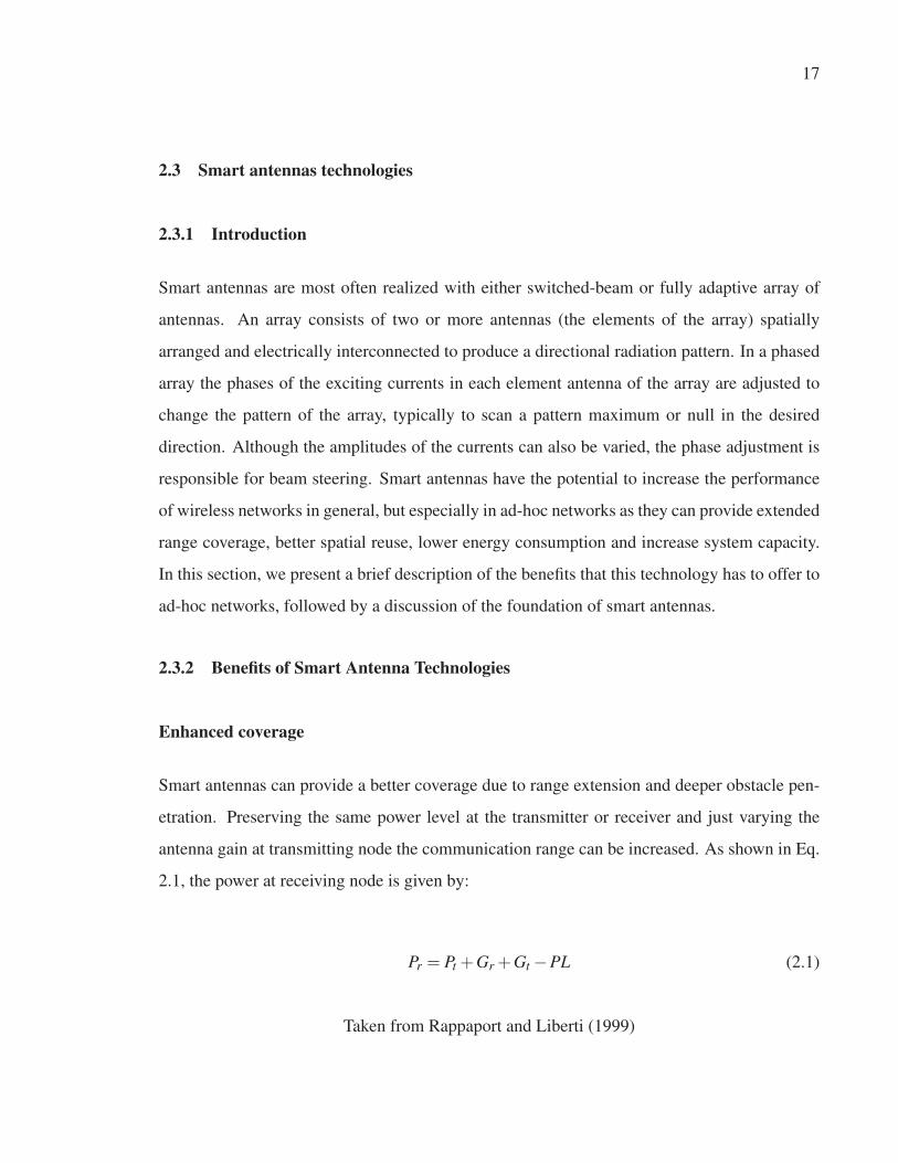
Enhanced coverage
Smart antennas can provide a better coverage due to range extension and deeper obstacle pen-
etration. Preserving the same power level at the transmitter or receiver and just varying the
antenna gain at transmitting node the communication range can be increased. As shown in Eq.
2.1, the power at receiving node is given by:
Pr = Pt +Gr +Gt −PL (2.1)
Taken from Rappaport and Liberti (1999)
18
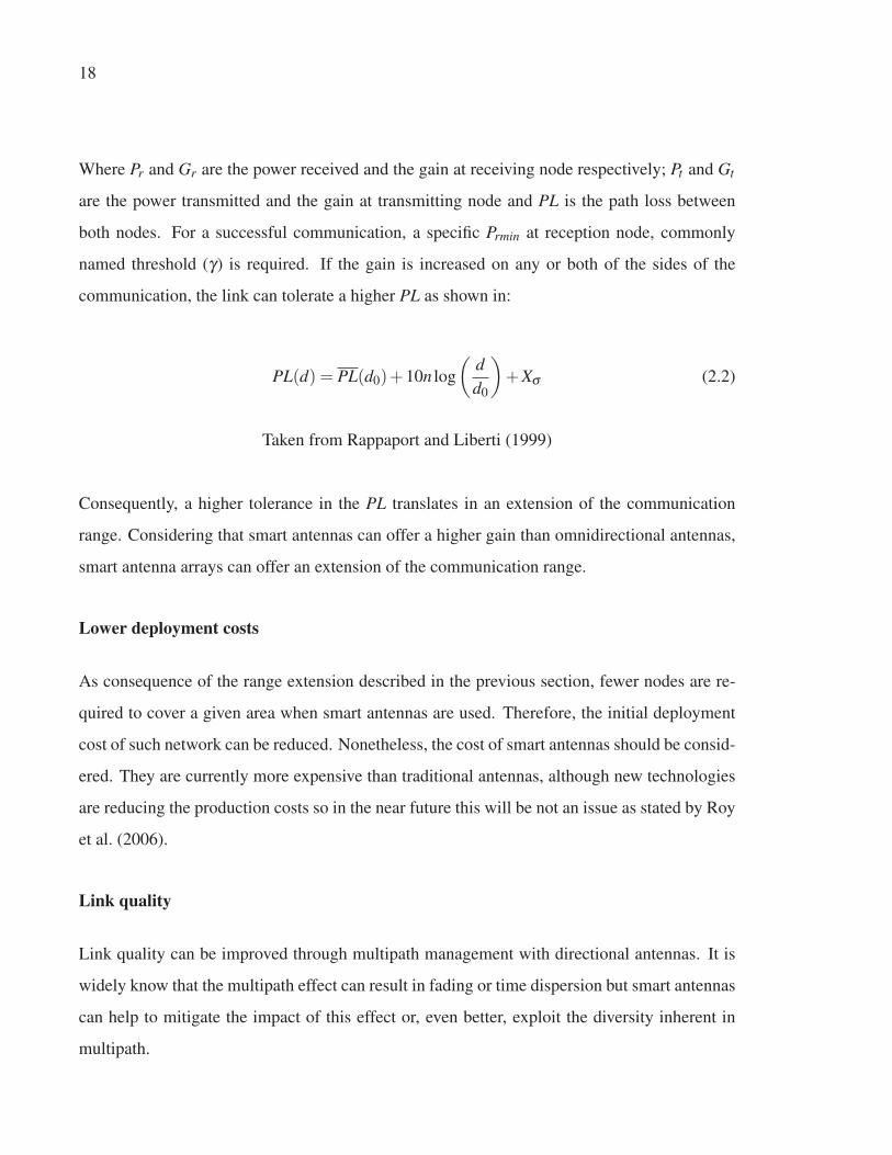
Where Pr and Gr are the power received and the gain at receiving node respectively; Pt and Gt
are the power transmitted and the gain at transmitting node and PL is the path loss between
both nodes. For a successful communication, a specific Prmin at reception node, commonly
named threshold (γ) is required. If the gain is increased on any or both of the sides of the
communication, the link can tolerate a higher PL as shown in:
PL(d) = PL(d0)+10n log
(dd0
)+Xσ (2.2)
Taken from Rappaport and Liberti (1999)
Consequently, a higher tolerance in the PL translates in an extension of the communication
range. Considering that smart antennas can offer a higher gain than omnidirectional antennas,
smart antenna arrays can offer an extension of the communication range.
Lower deployment costs
As consequence of the range extension described in the previous section, fewer nodes are re-
quired to cover a given area when smart antennas are used. Therefore, the initial deployment
cost of such network can be reduced. Nonetheless, the cost of smart antennas should be consid-
ered. They are currently more expensive than traditional antennas, although new technologies
are reducing the production costs so in the near future this will be not an issue as stated by Roy
et al. (2006).
Link quality
Link quality can be improved through multipath management with directional antennas. It is
widely know that the multipath effect can result in fading or time dispersion but smart antennas
can help to mitigate the impact of this effect or, even better, exploit the diversity inherent in
multipath.

19
Improved system capacity
Smart antennas can allow nodes in MANETs to operate at the same range as with omnidirec-
tional antennas but using less power. This in turns enables TDMA and FDMA systems to reuse
frequencies more often than systems with omnidirectional antennas, because the carrier to in-
terference ratio is greater when smart antenna systems are used. In other words, this increases
the number of users that can share the medium. Besides, smart antennas also allow separate
users spatially if using Spatial Division Multiple Access (SDMA). Since this approach allows
to allocate more users with a limited spectrum allocation, SDMA can lead to improved capacity
compared with conventional antennas.
2.3.3 Foundation of smart antenna technology
The term smart antenna typically refers to an array of low gain antennas connected to a sophis-
ticated signal processor (SP). This SP adapts the resulting beam to empathize signals of interest
or nulling interfering signals as shown in Figure 2.5. To simplify the analysis of antenna arrays,
we adopt the following assumptions(taken from Rappaport and Liberti (1999)):
• The space between the elements is small enough that there is no amplitude variation be-
tween the signals received at each element;
• There is no mutual coupling between elements;
• All incident fields can be decomposed into a discrete number of planes waves. In other
words, there are a finite number of signals;
• The bandwidth of the signal incident on the array is small compared with the carrier fre-
quency.

20
Figure 2.5 Smart directional antenna schematic
Adapted from Gross (2005, p. 66)
Linear Array
The Linear array is the simplest possible geometry array, where all elements are aligned along
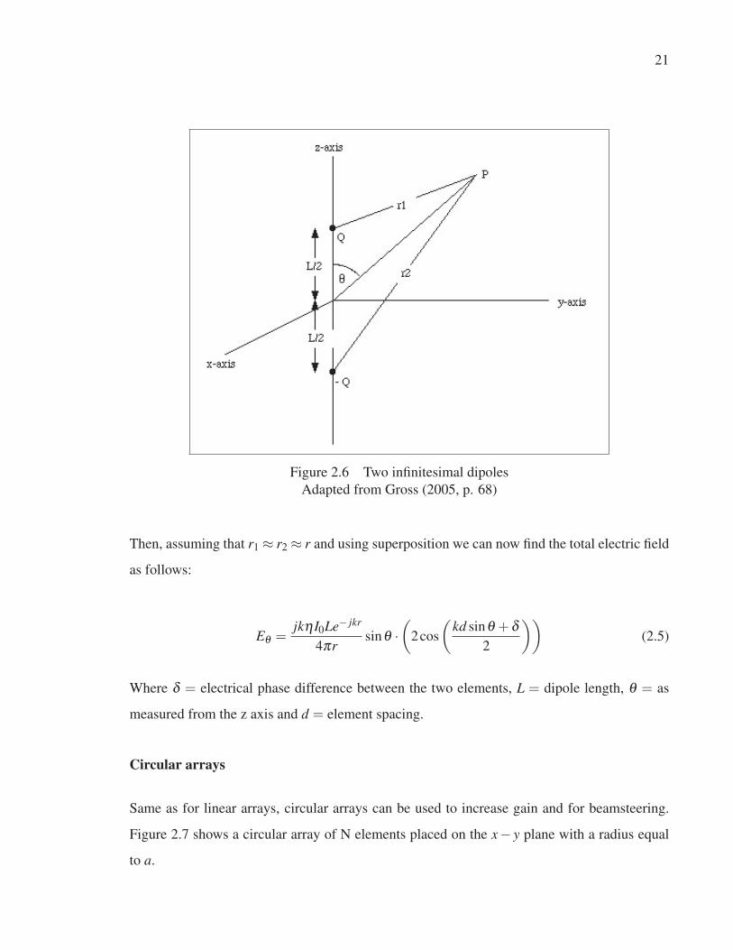
a straight line and have a uniform spacing between elements. Figure 2.6 depicts the minimum
array possible which is the 2-element array. This array is a good starting point to understand
the phase relationship between adjacent antenna elements.
Figure 2.6 shows two vertically polarized dipoles separated a distance L. The field point is
located at a distance r from the origin such that r >> L. We can, therefore assume that r,r1 and
r2 are approximately parallel to each other, so the following approximations are true:
r1 ≈ r+L2
sinθ (2.3)
r2 ≈ r− L2
sinθ (2.4)
21
Figure 2.6 Two infinitesimal dipoles
Adapted from Gross (2005, p. 68)
Then, assuming that r1 ≈ r2 ≈ r and using superposition we can now find the total electric field
as follows:
Eθ =jkηI0Le− jkr
4πrsinθ ·
(2cos
(kd sinθ +δ
2
))(2.5)
Where δ = electrical phase difference between the two elements, L = dipole length, θ = as
measured from the z axis and d = element spacing.
Circular arrays
Same as for linear arrays, circular arrays can be used to increase gain and for beamsteering.
Figure 2.7 shows a circular array of N elements placed on the x− y plane with a radius equal
to a.

22
Figure 2.7 Circular array of N elements
Adapted from Gopi Ram (2015)
The nth array element is at a distance a from the origin with angle φn. It is also possible to
associate a weight wn and phase δn to each element. As before we assume far field conditions
and that the point of observation is such that the position vectors are parallel or r1 ≈ r2 ≈ r.
The array factor can now be found in a similar fashion as was done with the linear array, as
follows:
AF =N
∑n=1
wne− j[kasinθ cos(φ−φn)+δn] (2.6)
where
φn =2πN
(n−1) = angular location o f each element (2.7)

23
Beamsteered circular arrays
The beamsteered circular array uses the same principle as linear beamsteered arrays but in this
array, we beamsteer the array to the angles (θ0, φ0). Therefore, the array factor is rewritten as:
AF =N
∑n=1
wne− j{ka[sinθ cos(φ−φn)−sinθ0 cos(φ−φ0)]} (2.8)
As an example, let us assume that all weights are uniform, and the array is steered to the angles
θ0 = 20°and φ0 = 0°. With N=10 and a= λ , we can plot the beamsteered circular array pattern
in 2-D as illustrated in Figure 2.8.
Figure 2.8 AF elevation pattern for beamsteered circular array (θ0 = 20°, φ0 = 0°)
Taken from Raviteja (2016)
24
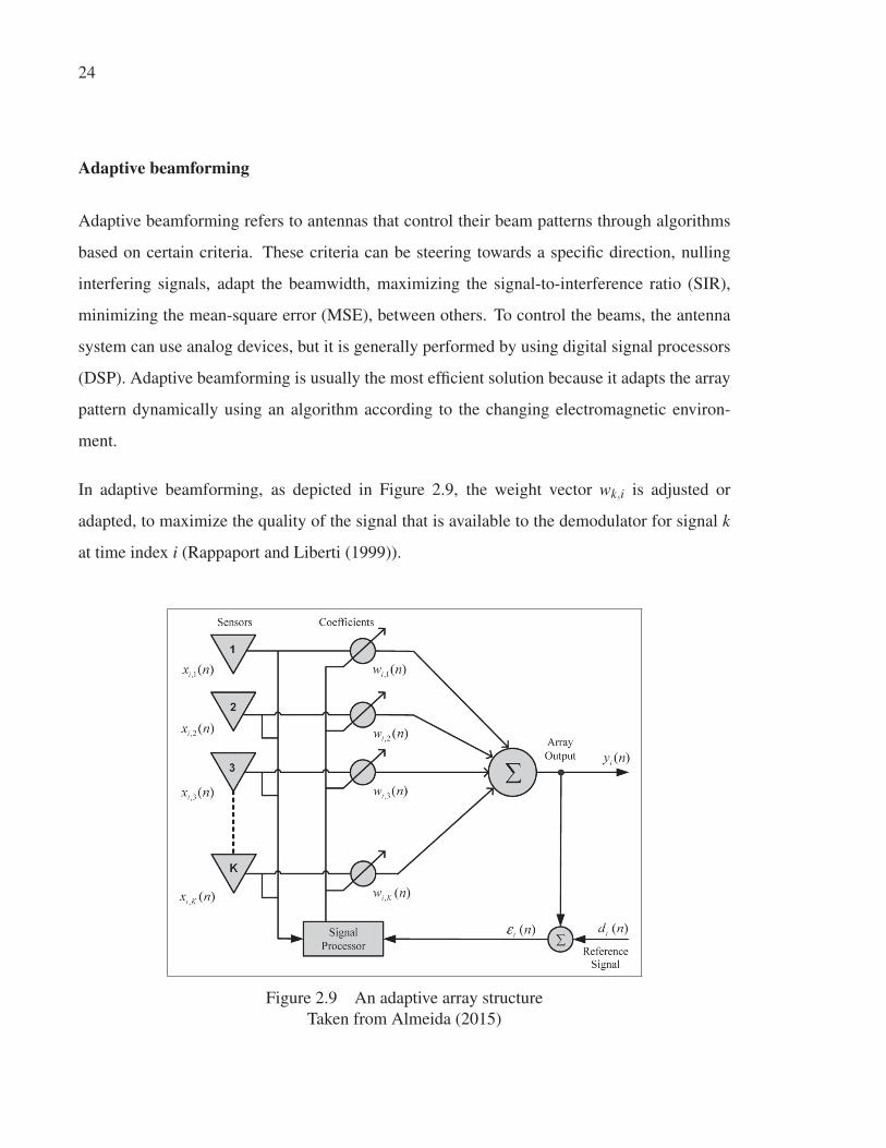
Adaptive beamforming
Adaptive beamforming refers to antennas that control their beam patterns through algorithms
based on certain criteria. These criteria can be steering towards a specific direction, nulling
interfering signals, adapt the beamwidth, maximizing the signal-to-interference ratio (SIR),
minimizing the mean-square error (MSE), between others. To control the beams, the antenna
system can use analog devices, but it is generally performed by using digital signal processors
(DSP). Adaptive beamforming is usually the most efficient solution because it adapts the array
pattern dynamically using an algorithm according to the changing electromagnetic environ-
ment.
In adaptive beamforming, as depicted in Figure 2.9, the weight vector wk,i is adjusted or
adapted, to maximize the quality of the signal that is available to the demodulator for signal k
at time index i (Rappaport and Liberti (1999)).
Figure 2.9 An adaptive array structure
Taken from Almeida (2015)
25
2.4 Literature Review
In this section, we summarize the most relevant research activities performed in the modeling
of ad-hoc networks using graph theory, recent advances in neighbor discovery and routing
algorithms using omnidirectional and directional antennas. We finish this section by reviewing
the state of the art of energy models for ad-hoc networks with omnidirectional and directional
antennas.
2.4.1 Modeling ad-hoc networks
In the past decade, wireless ad-hoc networks have attracted a lot of attention from the inter-
national research community. Extensive studies such as Gupta et al. (2008) and Zemlianov
and de Veciana (2005) have been performed to measure and improve the capacity and scalabil-
ity of these networks while others tried to adapt the existing MAC protocols to the changing
conditions of ad-hoc networks(Chen and Jiang (2007)).
Another aspect widely studied is the development and implementation of efficient routing pro-
tocols (Royer and Toh (1999), Maker and Chakeres (2000)) and more recently the implications
of nodes with selfish behaviors in the overall performance of the wireless network (Marbach
(2008)). Due to the absence of commercial solutions and the complexity of the ad-hoc sce-
narios, simulations have emerged as a widely accepted method to evaluate ad-hoc networks.
However, simulation models can not always provide a thorough understanding of the relation-
ship between network performance and specific parameters such as hop count, connectivity
or energy consumption. For this reason, many recent research efforts have considered the use
of mathematical models to describe the connectivity properties of wireless ad-hoc networks
better.
In literature, many researchers have proposed geometric random graphs as a mathematical
model to describe the connectivity properties of wireless ad-hoc networks better. The first
attempt to do so was proposed by Piret (1991) where the connectivity of two-dimensional radio
networks as a function of the range of the transmitters was addressed. This article’s results

26
shown that there is a critical range R that guarantees the connectivity of the network where R
is directly proportional to L (longitude of the square area) and D (node density). Later, Gupta
and Kumar (1998) developed another fundamental research on the minimum power required
to obtain a fully connected network. The authors found a relationship between the minimum
power required and the number of nodes (n) where n goes to infinity.
Another study performed by Bettstetter (2002) derived in an analytical expression that defines
the required radio r0 in a network with density ρ that almost assures that k nodes in the network
are connected (k − connected). For this purpose, a random placement of the nodes on the
evaluated area and a simple propagation model was assumed.
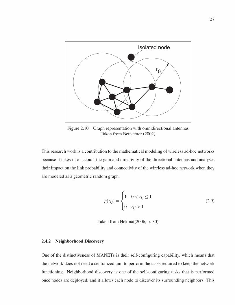
All the models mentioned above used the simple path loss propagation model in their assump-
tions. This means that the coverage area of each node is assumed as a perfect circular shaped
area around the node with radius R. Here, R is the distance where the received power is equal
to the receiver’s sensitivity γ as it is illustrated in Figure 2.10. Although this assumption is very
common, it is not realistic because it does not consider the randomness of the wireless channel.
This premise also assumes that the probability to have a link between any pair of nodes (i,j) or
the link probability (p(ri j)) is a simple step function as shown in Equation 2.9.
Later, Németh and Vattay (2003) pointed out that it is not accurate to model a wireless ad-
hoc network as a simple random graph because the link probability depends on the geometric
distance between the nodes. One of the consequences of this dependency is that the link proba-
bility between two nodes increases when they a have a common neighbor. This type of graphs
with a link dependency on the distance between nodes is referred in the literature as geometric
random graphs.
In an attempt towards a better modeling of wireless ad-hoc networks, recent studies like Bettstet-
ter (2004); Bettstetter and Hartmann (2005) proposed to consider the log-normal radio model
into the geometric random graph. This model is more realistic and suitable for ad-hoc networks
as it considers the medium scale radio signal power variations. However, all these previous
works considered omnidirectional transmissions on both sides of the ongoing communication.
27
Figure 2.10 Graph representation with omnidirectional antennas
Taken from Bettstetter (2002)
This research work is a contribution to the mathematical modeling of wireless ad-hoc networks
because it takes into account the gain and directivity of the directional antennas and analyses
their impact on the link probability and connectivity of the wireless ad-hoc network when they
are modeled as a geometric random graph.
p(ri j) =
⎧⎪⎨⎪⎩
1 0 < ri j ≤ 1
0 ri j > 1
(2.9)
Taken from Hekmat(2006, p. 30)
2.4.2 Neighborhood Discovery
One of the distinctiveness of MANETs is their self-configuring capability, which means that
the network does not need a centralized unit to perform the tasks required to keep the network
functioning. Neighborhood discovery is one of the self-configuring tasks that is performed
once nodes are deployed, and it allows each node to discover its surrounding neighbors. This

28
information is then used by the upper layer protocols such as topology control, medium access
control and routing protocol to perform their own tasks.
In recent years, a significant amount of research has been done in this area. For example,
Vasudevan et al. (2005); McGlynn and Borbash (2001); Keshavarzian et al. (2004); An and
Hekmat (2007) considered the type of antenna used. We gather from these articles that there
are two types of neighbor discovery algorithms depending on which antenna type is used: om-
nidirectional and directional neighbor discovery. The authors in McGlynn and Borbash (2001);
Keshavarzian et al. (2004) presented two algorithms for neighbor discovery in wireless ad-hoc
networks where nodes have omnidirectional antennas. While the algorithm proposed in McG-
lynn and Borbash (2001) can operate in asynchronous mode, synchronization is a requirement
for the algorithm described in Keshavarzian et al. (2004).
Previous research also proposed neighbor discovery algorithms using directional antennas.
In Vasudevan et al. (2005), the authors developed several algorithms considering three ap-
proaches: directional transmission and omnidirectional reception (DO); directional transmis-
sion and reception (DD); and omnidirectional transmission and directional reception (OD).
Each of these three strategies was first evaluated considering a direct discovery algorithm,
which means that a node discovers its neighbors only when it successfully hears a transmis-
sion from that neighbor. Then, the strategies mentioned before were evaluated considering a
gossip-based discovery algorithm where nodes gossip about each other’s location information
to speed up the discovery process. The gossip-based algorithm allows a node to discover its
neighbors indirectly and also allows a node to discover multiple neighbors in the same step.
The results of this work showed that those differences help nodes to discover their neighbors
significantly faster than using a non-gossip discovery algorithm.
The main drawback to gossip-based algorithms proposed so far is that they assume that each
node obtains its location information using a GPS device and if the number of nodes equipped
with GPS is reduced, the performance of the discovery algorithm also degrades correspond-
ingly. In An and Hekmat (2007) the authors introduced an original neighbor discovery algo-

29
rithm with directional antennas counting the mobility of the nodes and improving the energy
consumption. For the first problem, the cycle of the neighbor discovery is self-adapted accord-
ing to the dynamics of the network. Furthermore, to improve the power efficiency and reduce
overhead, the protocol can limit neighbor discovery attempts in regions where no new neigh-
bors are likely to be found. This work did not take into consideration multi-hop system and
only discovers one-hop neighbors.
Latterly, Zhang and Li (2008) proposed 2-way random neighbor discovery algorithms based
on the algorithms previously proposed by Vasudevan et al. (2005). Four algorithms were pro-
posed; two of them using omnidirectional antennas in certain stages of the algorithm and the
other two using directional antennas all the time. This work is limited because it does not
consider the gossip-based approach and for synchronization purposes, it requires the nodes to
have GPS devices.
Finally, in Ramanathan et al. (2005), the authors proposed several neighbor discovery methods
(NB) based on the usage of the directional antenna to transmit or receive data. According to
this paper, there are three kinds of NB methods: N-BF (without beamforming), T-BF (using
beamforming only on transmission) and TR-BF (using beamforming on transmission and re-
ception). Through simulations, the authors concluded that the use of beamforming on both,
transmission and reception offers a higher throughput due to the higher bandwidth available
when using directional antennas but it also increases the packet loss due to the synchronization
required in order to point both antennas on the same direction at the same time. However,
the solution where directional antennas are used for transmission and omnidirectional anten-
nas are used at reception offers a better-balanced performance. This is true because there is a
reduction in the total throughput of the network, but it is compensated with an improvement
in the packet loss ratio because a pointing mechanism is not needed when the omnidirectional
antennas are used for reception. Based on these results, we have also assumed an omnidirec-
tional or directional beamforming for transmissions and only omnidirectional beamforming at
reception.

30
2.4.3 Routing Algorithms
Since the first development of routing protocol for mobile ad-hoc networks, researchers have
shown their interest to support the routing decision based on the position of a node to increase
the packet delivery ratio and reduce the end-to-end delay. In the literature, there are several
implementations of both reactive and proactive routing protocols. In Ko and Vaidya (2000) the
authors proposed a reactive routing protocol called Location Aided Routing (LAR) that uses
the position information obtained by a GPS device to bound the search of a route to the defined
request zone. This zone is defined by the expected location of the destination node at the time
of the route discovery. Simulation results indicated that using location information resulted in
significantly lower routing overhead, as compared to other algorithms that do not use location
information. However, drawbacks of this approach are the need for GPS and the reactive nature
of the protocol which increases the setup delay of a route.
Basagni et al. (1998) proposed a proactive protocol where the nodes need the position infor-
mation from a GPS to calculate the route to destination. The entire network was divided into
hierarchical zones within which the information about the position of the nodes is distributed.
As in Ko and Vaidya (2000), this solution also depends on the GPS devices, besides the mo-
bility of the nodes between zones creates an unnecessary overload. In Quintero et al. (2007)
the authors developed Location-Enhanced On-Demand (LEOD) routing protocol, a framework
that uses the information provided by smart antennas to determine the position of the nodes in
the network and using this information, discover and maintain routes. The positioning algo-
rithm only considered one-hop neighbors and the method used to estimate the position is based
on the angle of arrival technique.
Studies of Dai and Zhao (2015) investigated the trade-off between directional and omnidi-
rectional antennas in terms of throughput improvement and end-to-end delay reduction. In
particular, the article investigated the effective transmission range of directional antennas and
the scaling rules of the delay due to the multi-hop routes in networks with only directional
antennas (DIR). Although the article demonstrated that there is a reduction in the end-to-end

31
delay, these results were expressed in an asymptotic notation giving only a general overview
of the network performance as a function of the number of nodes. It only considered static
nodes and the routing strategy is quite simple, choosing the next hop with the shortest dis-
tance to forwards a packet. In another recent paper, Chen et al. (2013) analyzed the achievable
throughput of MANETs when each node is equipped with directional antennas and a general
two-hop relay algorithm is adopted as routing scheme. The main contribution of this paper was
the development of a theoretical closed-form model to analyze the achievable throughput for
any specific antenna beamwidth θ and the optimal value of θ required to achieve the optimal
throughput.
Cobo et al. (2015) introduced a novel Location Based Routing Algorithm (LBRA) protocol,
that utilizes smart antennas to estimate node’s positions in the area covered by the network. The
proposed protocol takes routing decisions based on neighbor’s relative positions. Besides, it
uses the information about the battery charge remaining in the nodes to make power-aware rout-
ing decisions. Although the results showed that LBRA outperforms the Ad-hoc On-demand
Distance Vector (AODV) Perkins et al. (2003) protocol in terms of reducing the routing over-
head and incrementing the packet delivery rate, there is no evidence that the throughput and
end-to-end delay performed better that previous solutions. Additionally, the impact of the mo-
bility of the nodes was not addressed in this article.
Another article (Cheng et al. (2010)), proposed the Mobile Orthogonal Rendezvous Routing
Protocol (MORRP) which uses directional antennas to assist routing in highly mobile environ-
ments. In this article, the concept of Directional Routing Table (DRT) was introduced. MORRP
maintains a list of next hop based on probabilities to each interface direction which performs
well when the path lengths are short. For longer routes, it relies on route request (RREQ)
packets as in the traditional reactive routing protocols. Although MORRP seems to perform
better than traditional routing protocols, it has been only evaluated in square topologies and the
extended range of the directional beams was not exploited.

32
Many research efforts have demonstrated that the use of directional antennas for routing in
MANETs can improve the throughput and end-to-end delay of the wireless network. For ex-
ample, an experimental study in Ramanathan (2001) presented an improvement of up to 118%
in the average throughput, when directional antennas are used. Later, in Yi et al. (2003, 2007)
an analytical model demonstrated that is possible to obtain a throughput improvement in the
order of 2π/√
αβ in purely random networks and π2/αβ in arbitrary networks where α and β
are the antenna beamwidth for transmission and reception correspondingly. More recently, Li
et al. (2011) established an upper bound of Θ(√
logn/n)
and a lower bound of Ω(1/
√n logn
)on the maximum throughput that can be achieved in random networks with multi-hop relay
schemes.
Moreover, the delay as function of the number of the nodes in the network have been studied
in Dai et al. (2005) where a single channel model considering the path loss effect was used.
According to the authors, the delay D(n) is scales with Θ(√
n/ logn)
. Later in Dai and
Zhao (2015), a more comprehensive scenario is evaluated considering the large scale path
loss and the shadow fading effect as well as omnidirectional and directional antennas. The
results of this work have shown that the delay is reduced by a factor of (4/ tan2(θ/2))−2/α
when directional antennas are used in the network, where θ is the beam angle of the directional
antenna. Although the order sense function can help us to understand the impact of the growing
number of nodes the in network, it does not explain the actual achievable throughput and the
end-to-end reduction that can be achieved when directional antennas are used in the mobile
ad-hoc network. Besides, to the best of our knowledge, the reduction in the number of hops
between source and destination nodes due to the use of narrow beams and the position of the
nodes located in the second neighborhood of a node has not been previously investigated.
2.4.4 Energy Models
Wireless ad-hoc network are usually powered by batteries that have a limited life time. For
this reason, power efficiency is a critical issue in this type of networks. Energy issues have
been an active research topic since the first apparition of wireless ad-hoc networks. Most of the

33
previous work is focused on developing medium access control protocols to be energy efficient
in ad-hoc networks. For example, Singh and Raghavendra (1998) developed an extension of
the original MACA protocol with the addition of a separate signaling channel. The novelty
of the protocols is the conservation of power by turning off those nodes that are not actively
transmitting or receiving packets. Through simulations, the authors demonstrated that PAMAS
(Power Aware Medium Access Scheme) saves between 10 to 70% of power in fully connected
networks where the number of nodes is between 10 to 20. The proposed protocol does not
affect the delay and throughput performance of the traditional protocol.
In another article, Kranakis et al. (2005) explored the differences in power consumption of
ad-hoc networks when directional or omnidirectional antennas are used to connect at least k-
nodes. The proposed model assumed a random positioning of the nodes in a square area of
a unit length segment. Through simulations the authors proved that the energy consumption
required to maintain k-connectivity of the resulting network is lower when using directional
antennas instead of using omnidirectional antennas.
Spyropoulos and Raghavendra (2002) presented an energy-efficient routing and scheduling al-
gorithm to coordinate transmissions in ad-hoc networks. This study considered single beam
directional antennas installed in the nodes and implements the proposed solution in three steps.
First, the shortest path with minimum energy consumption are calculated. Then the maximum
amount of traffic than can be transported is estimated and finally the transmissions are sched-
uled trying to minimize the time of connection between transmitter and receiver. The problem
was formulated using graph theory and through simulations, the authors have demonstrated
that the proposed routing scheme is more efficient than traditional protocols in terms of energy
cost for routing.
Later, Dai et al. (2005) proposed four algorithms for routing tree construction that take ad-
vantage of directional antennas. An important contribution of this paper is the assumption
that antennas have an adjustable beam angle. It also allows the nodes to control the irradiated
power so it can be increased to reach farthest nodes. The simulation results showed that when

34
the nodes are relatively sparse and the beam angle is small, the linear insertion (LI) algorithm
outperforms the others.
More recently, Zhu et al. (2006) developed an energy consumption model for common MAC
Protocols (CSMA,MACA and 802.11) that takes into account energy consumption due to
packet transmissions as well as control packets and retransmissions. The authors verified by
simulations that the proposed model match the actual energy consumption much better than
the existing models. The results of this paper also showed that the proposed energy model
could be used to determine paths with minimum energy cost and thus achieving better energy
conservation performance than other models.
Finally, in Zhu and Wang (2011) the authors investigated the energy consumed by routing over
MANETs. They remarked that without a careful design, some energy-efficient routing algo-
rithms can perform worse than traditional routing protocols. Although the proposed scheme
(PEER) demonstrated that it improves the performance during path discovery and it also used
several mobile scenarios, it assumed the use of omnidirectional antennas only. We consider that
it will be interesting to derive an extension of the link cost model proposed by these authors to
include the directionality of smart antennas in ad-hoc networks.

CHAPTER 3
MODELING DIRECTIONALITY IN WIRELESS AD-HOC NETWORKS
3.1 Introduction
Wireless ad-hoc networks are deployed without a fixed infrastructure or central controllers
such as access points or base stations. In these networks, data packets are forwarded directly to
the destination if they are within the transmission range of the sender or sent through a multi-
hop path of intermediary nodes that act as relays. This paradigm, where a fixed infrastructure
is not needed, is tolerant to topology changes and allows a fast deployment is suitable for a
large number of network implementations, such as mobile hand-held devices, wireless sensors,
disaster recovery networks, etc.
In recent years, smart directional antennas have been identified as a robust technology that
can boost the performance of wireless ad-hoc networks in terms of coverage, connectivity,
and capacity. Contrary to omnidirectional antennas which irradiate energy in all directions,
directional antennas can focus the energy in a specific direction, extending the coverage range
for the same irradiated power. Longer ranges provide shorter paths to destinations and im-
prove connectivity. Moreover, directional antennas can reduce the collision probability in a
contention-based access scheme as they can steer the main lobe in the desired direction and set
nulls in all the others, thereby they minimize the co-channel interference and reduce the noise
level. Connections are more reliable due to the increased link stability and spatial diversity.
Shorter paths, as well as alternative paths, are also available as a consequence of the use of
directional antennas. All these features combined results in a higher network capacity.
In this chapter, we investigate the impact of smart antennas in the connectivity of wireless ad-
hoc networks. To take into consideration this property, we assume directional transmissions
on the link probability function that is used to set the weight of the edges in the graph that
represents the wireless ad-hoc network. The rest of the chapter is organized as follows: First,
we introduce graph theory and its applications to multi-hop networks, then we describe the

36
system model assumptions made in our research and the proposed model, we continue with the
simulations setup, and we finish the chapter with an analysis of the obtained results.
3.2 Graph theory and Ad-hoc Networks
The topologies of ad-hoc networks are constantly changing due to nodes’ movements and radio
signal variations. However, from the topology point of view a wireless ad-hoc network can be
represented as a graph G(V, E) where the nodes correspond to the vertices of the graph and the
links between the nodes correspond to the edges of the graph.
To better understand the relationships that happens on graph representations of ad-hoc net-
works, it is necessary to define the following terms:
• The number of direct neighbors of a given node is defined as the degree of the node;
• A graph G is connected if at least exist a path {i... j} between any pair of nodes i and j.
When there is no path between any pair of nodes, the network is said to be disconnected;
• The hop count specifies the number of hops on a path between any pair of source-destination
nodes;
• The average hop count is the mean value of the number of hops between all the possible
source-destination pairs in the network.
3.3 System Model
In this section, we will describe the considerations made in our model. We begin with the node
distribution model which is a description on how we have placed the nodes over the area to be
analyzed, then we describe the antenna model, and we finalize this section with a description
of the wireless channel model assumed in this research work.

37
3.3.1 Node Distribution Model
We consider that nodes are uniformly distributed over a square shaped service area of length
M; therefore, the coverage area is defined as Ω = M ×M and the node density is defined as
d = N/Ω where N is the total number of nodes.
3.3.2 Network Topology
In real scenarios nodes are positioned on a three-dimensional space (xi,yi,zi). In order to
simplify our analysis and following a commonly accepted assumption made in several previous
works we have decided to use a two dimensional array (xi,yi) with N columns where N is equal
to the number of nodes in the network. The network topology of the area to be studied is the
represented as showed on Table 3.1
Table 3.1 Position of the nodes array
ID 1 2 3 ... NX pos x1 x2 x3 ... xNY pos y1 y2 y3 ... yN
3.3.3 Antenna model
In general terms, an antenna is a device that is capable of radiating or collecting radio signals
in all directions (omnidirectional case) or in a specific direction (directional case). Tradi-
tional wireless networks are equipped with omnidirectional antennas, but recently the research
community has pointed out that directional antennas can improve the performance of such net-
works. A directional antenna can have a larger range compared to an omnidirectional antenna
due to its directivity. The antenna gain is used to quantify the directionality of an antenna. For
a given direction �d, the gain of a directional antenna is defined as:
G(�d)=
ηU(�d)Uavg
(3.1)

38
Where U(�d) is the power density in the direction of �d, Uavg is the average power density over
all directions, and η is a parameter used to define the antenna efficiency and represents the
losses related to hardware design. In this work, we assume that all the nodes in the network
are equipped with a switched beamforming antenna array of N elements, the main lobe of each
element is represented as a conical segment of 2π/N radians. For convenience, we assume
that the gain of the side lobes is insignificant. We also assume that the antenna elements do
not overlap and cover the entire plane when all them are used at the same time. We numbered
the elements from 1 to N starting with the element located in the east (3 o’clock) position,
following the same convention used in Zhou et al. (2007) as shown in Figure 3.1.
Figure 3.1 Antenna array installed in wireless nodes

39
3.3.4 Wireless Channel Model
In radio communications, the power transmitted decreases according to the distance traveled
to the destination. This fact is called path loss, and according to Rappaport, Theodore (2002),
it follows a power law that can be represented as:
Pa(r) = c(
rr0
)−η(3.2)
Where r0 is a reference distance1, the parameter η is commonly referred as the path loss ex-
ponent which can take values from 2 in free space to 6 in highly dense urban environments.
The constant c depends on the transmitted power, gains of transmitting and receiving antennas,
and the wavelength of the signal. As we are interested in the impact of the antenna gains, we
rewrite the equation 5.2 in terms of the antenna gains as follows:
Pa(r) = PtGtGr
(rr0
)−η(3.3)
According to the log-normal path loss model, the power received at node j from node i with a
distance ri j between them is equal to:
10log10
(P(ri j
))= 10log10
(Pa
(ri j
))+ x (3.4)
Where x is a zero-mean normally distributed random variable (in dB) with standard deviation
σ (also in dB). Notice that when σ = 0 the log-normal model reduces to the path loss model.
Moreover, the condition to establish a link between two nodes is than the received power is
greater that the receiver’s sensitivity γ , therefore, the distance R where Pa(r) is equal to γ
is calculated using the Equation 5.2. In other words γ = (R/r0)−η . Following the method
1 This distance is typically chosen to be 1m in indoor environments and 100 meters or 1 kilometer in outdoors
Rappaport, Theodore (2002).
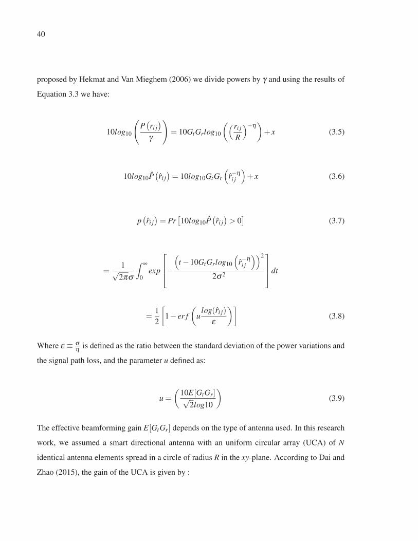
40
proposed by Hekmat and Van Mieghem (2006) we divide powers by γ and using the results of
Equation 3.3 we have:
10log10
(P(ri j
)γ
)= 10GtGrlog10
((ri j
R
)−η)+ x (3.5)
10log10P(ri j
)= 10log10GtGr
(r−η
i j
)+ x (3.6)
p(ri j
)= Pr
[10log10P
(ri j
)> 0
](3.7)
=1√
2πσ
∫ ∞
0exp
⎡⎢⎣−
(t −10GtGrlog10
(r−η
i j
))2
2σ2
⎤⎥⎦dt
=1
2
[1− er f
(u
log(ri j)
ε
)](3.8)
Where ε ≡ ση is defined as the ratio between the standard deviation of the power variations and
the signal path loss, and the parameter u defined as:
u =
(10E[GtGr]√
2log10
)(3.9)
The effective beamforming gain E[GtGr] depends on the type of antenna used. In this research
work, we assumed a smart directional antenna with an uniform circular array (UCA) of N
identical antenna elements spread in a circle of radius R in the xy-plane. According to Dai and
Zhao (2015), the gain of the UCA is given by :
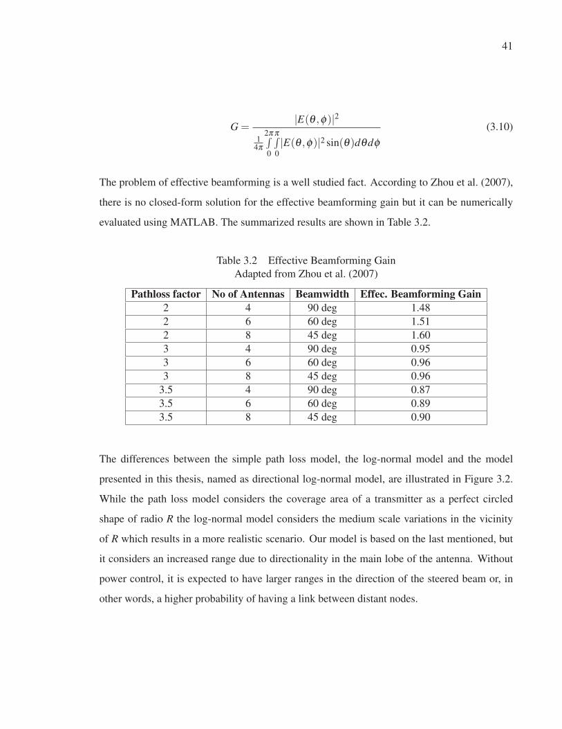
41
G =|E(θ ,φ)|2
14π
2π∫0
π∫0
|E(θ ,φ)|2 sin(θ)dθdφ(3.10)
The problem of effective beamforming is a well studied fact. According to Zhou et al. (2007),
there is no closed-form solution for the effective beamforming gain but it can be numerically
evaluated using MATLAB. The summarized results are shown in Table 3.2.
Table 3.2 Effective Beamforming Gain
Adapted from Zhou et al. (2007)
Pathloss factor No of Antennas Beamwidth Effec. Beamforming Gain2 4 90 deg 1.48
2 6 60 deg 1.51
2 8 45 deg 1.60
3 4 90 deg 0.95
3 6 60 deg 0.96
3 8 45 deg 0.96
3.5 4 90 deg 0.87
3.5 6 60 deg 0.89
3.5 8 45 deg 0.90
The differences between the simple path loss model, the log-normal model and the model
presented in this thesis, named as directional log-normal model, are illustrated in Figure 3.2.
While the path loss model considers the coverage area of a transmitter as a perfect circled
shape of radio R the log-normal model considers the medium scale variations in the vicinity
of R which results in a more realistic scenario. Our model is based on the last mentioned, but
it considers an increased range due to directionality in the main lobe of the antenna. Without
power control, it is expected to have larger ranges in the direction of the steered beam or, in
other words, a higher probability of having a link between distant nodes.

42
Figure 3.2 Different link models and resulting network topologies
3.4 Simulation Setup
Our simulations were carried out in Matlab version R2013A, we have evaluated the link prob-
ability of our log-normal model with directional antennas and compared with the omnidirec-
tional log-normal model. In the first experiment, ten nodes were uniformly distributed over an
M ×M square shaped area, where M is equal to 2000m. In this experiment, we assumed om-
nidirectional antennas for transmission and reception. Nodes have a coverage radius of 200m
and we considered a path loss exponent η = 3.5. Once the nodes are deployed over the area
to be studied, the neighbor list is generated using the Find Neighbors function described in
Algorithm 3.1. Then, paths from every node to all the others are constructed using the Di-
jkstra shortest path algorithm. This experiment was repeated under the same conditions but
increasing the number of nodes from 10 to 100 with a step of 10 nodes {10,20, ...,100}. On
each iteration, the position of the nodes was cleared and then uniformly distributed again. We
also considered an ideal MAC layer which means that there is the same probability of having a
successful transmission or collision. If a collision occurs, the packet is lost as retransmissions
are not considered.
In the second experiment, we considered directional transmissions by introducing the log-
normal link probability model with directional antennas. As in the first experiment, ten nodes
were uniformly distributed over a 2000m×2000m square shaped area. We consider directional
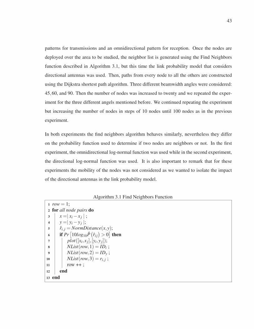
43
patterns for transmissions and an omnidirectional pattern for reception. Once the nodes are
deployed over the area to be studied, the neighbor list is generated using the Find Neighbors
function described in Algorithm 3.1, but this time the link probability model that considers
directional antennas was used. Then, paths from every node to all the others are constructed
using the Dijkstra shortest path algorithm. Three different beamwidth angles were considered:
45,60, and 90. Then the number of nodes was increased to twenty and we repeated the exper-
iment for the three different angels mentioned before. We continued repeating the experiment
but increasing the number of nodes in steps of 10 nodes until 100 nodes as in the previous
experiment.
In both experiments the find neighbors algorithm behaves similarly, nevertheless they differ
on the probability function used to determine if two nodes are neighbors or not. In the first
experiment, the omnidirectional log-normal function was used while in the second experiment,
the directional log-normal function was used. It is also important to remark that for these
experiments the mobility of the nodes was not considered as we wanted to isolate the impact
of the directional antennas in the link probability model.
Algorithm 3.1 Find Neighbors Function
1 row = 1;
2 for all node pairs do3 x =| xi − x j | ;
4 y =| yi − y j |;5 ri, j = NormDistance(x,y);6 if Pr
[10log10P
(ri j
)> 0
]then
7 plot([xi,x j], [yi,y j]);8 NList(row,1) = IDi ;
9 NList(row,2) = IDy ;
10 NList(row,3) = ri, j ;
11 row ++ ;
12 end13 end

44
3.5 Analysis of Results
In this section, we present the results of our simulations as they were described in the previous
section. We also discuss the main findings that we identified during this process. In order to
keep concordance with the proposed solution, we have divided this task into two sections: the
impact of directional antennas on the link probability model, and the hop count analysis.
3.5.1 Link Probability
The aim of this section is identifying the impact of the directional antennas (by considering
the antenna gains) in the link probability model. Figure 3.3 depicts the results of our simula-
tions regarding link probability. We present the results for antenna arrays with four elements
(90°each element), six elements (60°per element) and eight elements (45°each element). The
omnidirectional model is also presented here to compare versus the directional model. Two om-
nidirectional models were considered: the simple path loss model and the log-normal model.
As we find in Section 3.3.4 the simple path loss model is a step function that represents the fact
that any node inside the coverage area of a given node is connected to the node and any node
outside this area has no connectivity with the node. This finding is represented in the figure as
a step function at normalized distance d = 1 with probability p = 1 for any distance d < 1 and
probability p = 0 for any distance d > 1.
Then, in Figure 3.3a we observe that as we increase the number of elements in the antenna array
or, in other words as we narrow the antenna beam, the probability of having a link at greater
distances than the normalized distance d = 1 increases compared with the omnidirectional case.
This is an important finding because it demonstrates that as we narrow the beam of the antenna
and the energy is focused in a particular direction we have an increment in the antenna range.
As a consequence, the antenna is capable of reaching farthest nodes that are then included
in the list of neighbors. If the number of reachable neighbors increases for a given node, it
means that this node has increased its connectivity. Therefore, the full network connectivity is
improved because more links are available and more alternative paths are available to construct

45
0 2 4 6 80
0.1
0.2
0.3
0.4
0.5
0.6
0.7
0.8
0.9
1
normalized distance
link
prob
abili
ty
pathlossomni−directionalN = 4 θ = 90 degN = 6 θ = 60 degN = 8 θ = 45 deg
a)
2 2.5 3 3.5
0.05
0.1
0.15
0.2
0.25
normalized distance
link
prob
abili
ty
pathlossomni−directionalN = 4 θ = 90 degN = 6 θ = 60 degN = 8 θ = 45 deg
b)
Figure 3.3 Link probability comparisons

46
the routes to destinations. To remark the increase on link probability, on Figure 3.3b we have
zoom-in the values around the normalized distance=2.
Taking as an example the results around the normalized distance n=2 (twice the threshold
range with omnidirectional antennas), we found that the probability of having a link between
two nodes increases approximately 46% when we consider the directionality of the antennas.
While around the normalized distance n=3 (three times the threshold range) the probability
increases up to 78%. This result means that the model is correctly illustrating what we expect
to find in a real scenario: with extended ranges consequence of the directional antennas, nodes
that are farthest can be reached which translates in a better-connected network.
Finally, we point out that for normalized distance lower than d = 1, our model shows a slightly
lower probability than the omnidirectional models. This can be explained as a consequence
of the use of directional antennas because it is true that as we narrow the antenna beam, we
have observed a higher probability of connection for longer distances as a consequence of
the directivity of the antenna. Unfortunately, it also means that nodes that are closer to the
transmitter, but in a different direction where the main lobe of the node is pointing, can appear
as unconnected because they are outside the coverage area of the transmitting node. This last
observation is commonly referred in the literature as the spatial diversity.
3.5.2 Hop count
To evaluate the impact of our model on the hop count, we have uniformly distributed 100 nodes
in a square-shaped area of length equal to 2000 m. Then we used the link probability defined
by Equation 4.5 to create links between the nodes. Once the links were created, we called the
function Find Neighbors to identify all the possible paths between source and destination. We
have considered four scenarios: omnidirectional transmissions (effective gain=1), and three
directional scenarios with 4,6 and 8 antenna elements.
Figure 3.4 shows the resultant network graphs. Fig 3.4a represents the omnidirectional case,
Fig 3.4b shows the results when 4-elements smart antennas are used. Fig 3.4c represents the
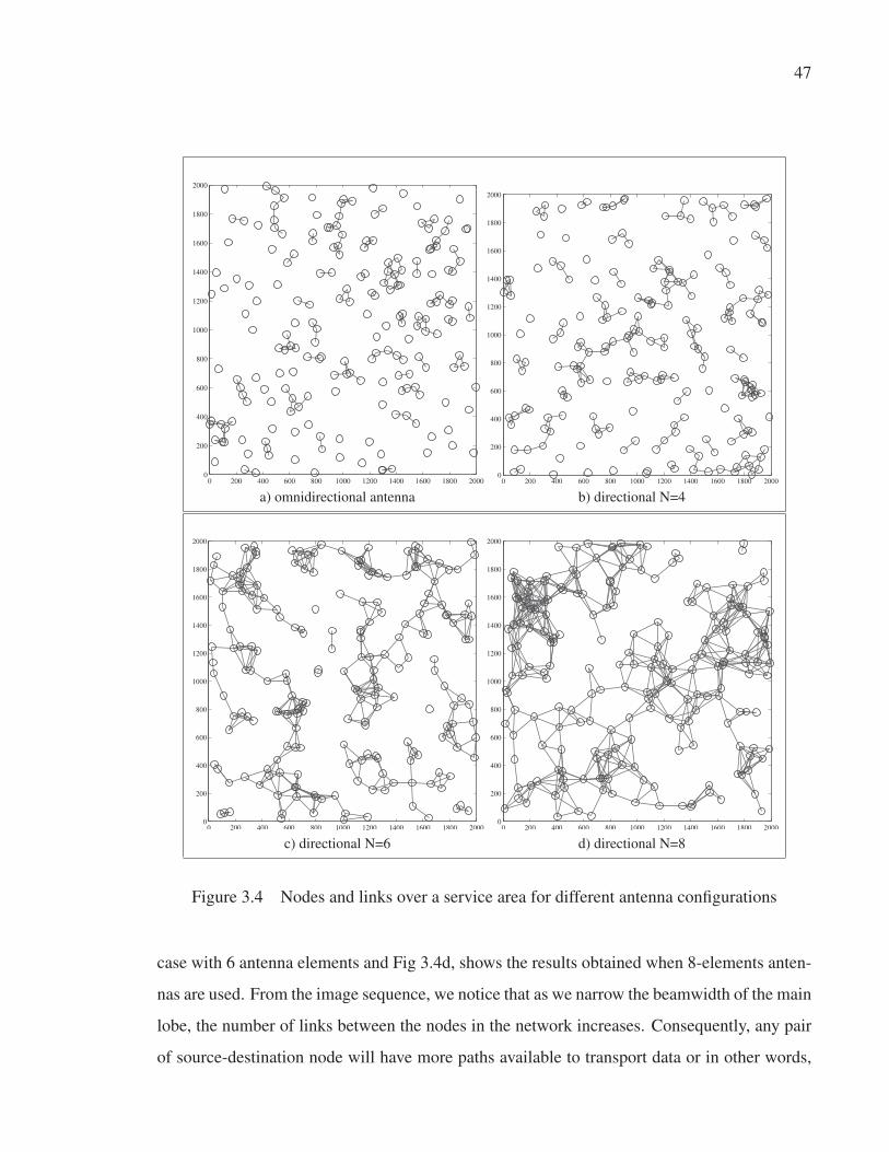
47
0 200 400 600 800 1000 1200 1400 1600 1800 20000
200
400
600
800
1000
1200
1400
1600
1800
2000
a) omnidirectional antenna
0 200 400 600 800 1000 1200 1400 1600 1800 20000
200
400
600
800
1000
1200
1400
1600
1800
2000
b) directional N=4
0 200 400 600 800 1000 1200 1400 1600 1800 20000
200
400
600
800
1000
1200
1400
1600
1800
2000
c) directional N=6
0 200 400 600 800 1000 1200 1400 1600 1800 20000
200
400
600
800
1000
1200
1400
1600
1800
2000
d) directional N=8
Figure 3.4 Nodes and links over a service area for different antenna configurations
case with 6 antenna elements and Fig 3.4d, shows the results obtained when 8-elements anten-
nas are used. From the image sequence, we notice that as we narrow the beamwidth of the main
lobe, the number of links between the nodes in the network increases. Consequently, any pair
of source-destination node will have more paths available to transport data or in other words,
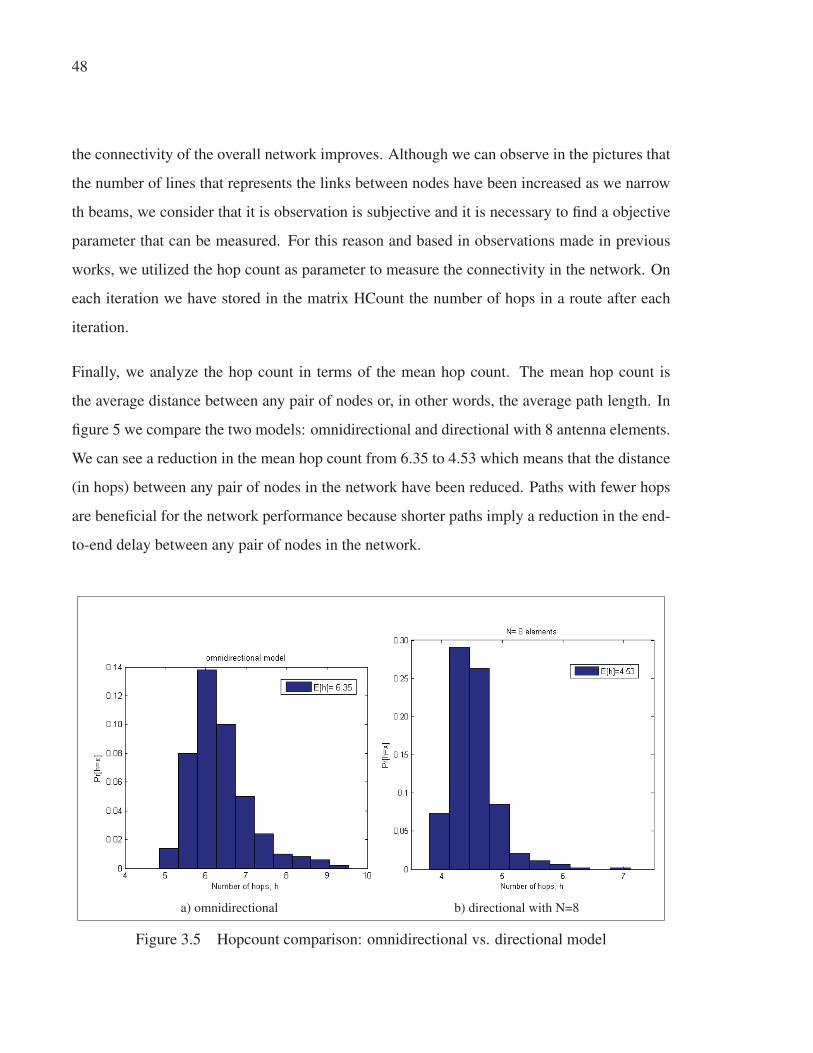
48
the connectivity of the overall network improves. Although we can observe in the pictures that
the number of lines that represents the links between nodes have been increased as we narrow
th beams, we consider that it is observation is subjective and it is necessary to find a objective
parameter that can be measured. For this reason and based in observations made in previous
works, we utilized the hop count as parameter to measure the connectivity in the network. On
each iteration we have stored in the matrix HCount the number of hops in a route after each
iteration.
Finally, we analyze the hop count in terms of the mean hop count. The mean hop count is
the average distance between any pair of nodes or, in other words, the average path length. In
figure 5 we compare the two models: omnidirectional and directional with 8 antenna elements.
We can see a reduction in the mean hop count from 6.35 to 4.53 which means that the distance
(in hops) between any pair of nodes in the network have been reduced. Paths with fewer hops
are beneficial for the network performance because shorter paths imply a reduction in the end-
to-end delay between any pair of nodes in the network.
a) omnidirectional b) directional with N=8
Figure 3.5 Hopcount comparison: omnidirectional vs. directional model
49
In this chapter we investigated the impact of directional antennas on the modeling of wireless
ad-hoc networks. Specifically, we proposed a novel link probability model that considers the
directional gain of the smart antenna arrays. Through simulations, we have demonstrated that
it is possible to achieve a higher network connectivity when directional antennas are consid-
ered into the model. We have also demonstrated that as the main lobe of the antenna array is
narrowed the probability to have a link with nodes that are farthest is higher when the effective
gain of the antennas is considered. In terms of the hopcount, we have also noticed a reduction
in the mean hopcount when the directional model is used. He have also verified that fewer
hops in any path between a source and destination node leads to an improved performance as
was previously presented by Dai and Zhao (2015) because less hops in a route implies less
delay as consequence of the message processing on each node in the route and time spent in
propagation.
Mobility of the nodes was not considered in this section as we wanted to aisle the impact
of directional antennas in the link probability mode for ad-hoc networks. We consider that
mobility is an important factor to analyze and it will be interesting to include in a future anal-
ysis. Further, we also notice that the mathematical model considered in our analysis contains
some simplifying assumptions including: first, the directional antenna gain is a constant in its
mainlobe; second, the transmission distance is uniform over all directions within the mainlobe;
third, a uniform transmission rate is assumed by all communications. Removing any of the
above simplifications in the analysis will provide a more realistic model and can be a very in-
teresting future direction. Besides, this model is a fundamental study that contributes into the
mathematical model of ad-hoc networks but it will be interesting to analyze the impact of di-
rectional antennas in a more realistic scenario. For example, instead of using the shortest path
algorithm to calculate the routes between source and destination will be interesting to evaluate
the performance when a reactive protocol such as AODV is used. Finally, in this section we
considered the extended range that can be achieved when the beams are narrowed and we used
fixed beams (45°, 60°and 90°). It is of particular interest to evaluate the improvements in the

50
performance of the network if the beam can be selected as required (adaptive beams). All this
interesting and open research questions will be addressed in the next chapter.

CHAPTER 4
NEIGHBOR DISCOVERY AND ROUTING SCHEMES FOR AD-HOC NETWORKS
4.1 Introduction
A mobile ad-hoc network (MANET) is a self-organized, infrastructure-less set of nodes that
can communicate with each other over wireless links. The rapid deployment, low cost, and
robustness of this type of networks are key features that are very appealing for applications
like military and recovery disaster networks, wireless sensor networks, vehicular networks and
many similar others. In infrastructure networks, such as cellular networks, the communications
are performed on a one hop basis between the base station and the mobile station, whereas in
ad-hoc networks two nodes are commonly connected through multiple hops. This means that
nodes in these networks also forward packets acting as relays. For these reasons routing in
such networks is a challenging task that can not be performed by the same routing protocols
developed for wired networks.
Traditional routing protocols for MANETs were initially designed and developed considering
omnidirectional antennas installed on the nodes. However, recent studies have suggested that
the use of directional antennas can considerably increase the throughput of these wireless net-
works. In this article, we introduce a novel routing algorithm for MANETs where the wireless
nodes are fitted with smart directional antennas. The algorithm aims to take full advantage of
the beamforming features of smart antennas. The primary objective of our routing algorithm
is to reduce the number of hops in the route between a source and destination node by using
the location information of the nodes participating into the routing path gathered during the
neighbor discovery process. In this work, we refer to the location as the last angular sector
where the node was seen. This information is taken from the antenna element used to discover
the node. Although the location information obtained by this mechanism is not as precise as
a GPS positioning system, we can use it as a first step for a more complex location system
which also uses the information provided by the neighbor discovery algorithm proposed in this

52
work. This method can be handy when devices are located in dense areas (e.g., downtown,
inside a building, at underground commercial complexes), on devices without a GPS or within
particular application networks such as disaster discovery networks, unmanned aerial vehicle
networks, and firefighting robot networks.
When it is time to select the next hop of the routing path, the decision-making process in
the algorithm is supported by a novel neighborhood discovery process also proposed in this
article. During the neighborhood discovery, a four-way handshake method is used where the
nodes interchange the antenna sector used to discover each other. The capability of controlling
the range and coverage by varying the beam width angle is used in our algorithm to limit the
neighborhood search in the vicinity of a node. In this chapter we present:
• A gossip neighborhood discovery algorithm that uses the information provided by direc-
tional antennas to discover neighbors in the second neighborhood of the node using direc-
tional beams;
• A routing algorithm that aims to reduce the number of hops during the route construction
using the information provided by the neighborhood discovery algorithm also proposed in
this article and;
• A comprehensive comparison between the scheme suggested in this article and similar
solutions previously developed.
4.2 Overview
4.2.1 Neighbor Discovery
One of the distinctiveness of MANETs is their self-configuring capability, which means that
the network does not need a centralized unit to perform the tasks required to keep the network
functioning. Neighborhood discovery is one of the self-configuring tasks that is done once
nodes are deployed; it allows each node to discover its surrounding neighbors. Then, this in-

53
formation is used by the upper layer protocols such as topology control, medium access control
and routing protocol to perform their tasks. A lot of research has been done in this area. For
example, Vasudevan et al. (2005); McGlynn and Borbash (2001); Keshavarzian et al. (2004);
An and Hekmat (2007) considered the type of antenna used. We gather from these articles
that there are two types of neighbor discovery algorithms depending on which antenna type is
used: omnidirectional and directional neighbor discovery. McGlynn and Borbash (2001) and
Keshavarzian et al. (2004) present two algorithms for neighbor discovery in wireless ad-hoc
networks where nodes have omnidirectional antennas. While the algorithm proposed in McG-
lynn and Borbash (2001) can operate in asynchronous mode, synchronization is a requirement
for the algorithm described in Keshavarzian et al. (2004).
Previous research also suggested neighbor discovery algorithms using directional antennas. In
Vasudevan et al. (2005), the authors develop several algorithms considering three approaches:
directional transmission and omnidirectional reception (DO); directional transmission and re-
ception (DD); and omnidirectional transmission and directional reception (OD). Each of these
three strategies is first evaluated considering a direct discovery algorithm, which means that a
node discovers its neighbors only when it successfully hears a transmission from that neighbor.
Then, the strategies mentioned before are evaluated considering a gossip-based discovery al-
gorithm where nodes gossip about each other’s location information to speed up the discovery
process. The gossip- based algorithm allows a node to discover its neighbors indirectly and also
allows a node to discover many neighbors in the same step. The results of this work showed
that those differences help nodes to discover their neighbors significantly faster than using a
non-gossip discovery algorithm. The main drawback to gossip-based algorithms proposed so
far is that they assume that each node obtains its location information using a GPS device and,
if the number of nodes equipped with GPS is reduced, the performance of the discovery al-
gorithm also degrades correspondingly. In An and Hekmat (2007) the authors introduce an
original neighbor discovery algorithm with directional antennas counting the mobility of the
nodes and improving the energy consumption. For the first problem, the cycle of the neighbor
discovery is self-adapted according to the dynamics of the network. Further, to improve the

54
power efficiency and reduce overhead, the protocol can limit neighbor discovery attempts in
regions where no new neighbors are likely to be found. This work does not take into consider-
ation multi-hop system and only discovers one-hop neighbors.
Latterly in Zhang and Li (2008) the authors describe 2-way random neighbor discovery al-
gorithms based on algorithms proposed in Vasudevan et al. (2005). Four algorithms were
proposed; two of them using omnidirectional antennas in certain stages of the algorithm and
the other two using directional antennas all the time. The shortcoming of this work is that it
does not consider the gossip-based approach and for synchronization purposes, it requires the
nodes to have GPS devices.
Finally, Ramanathan et al. (2005) proposed several neighbor discovery methods(NB) based on
the usage of the directional antenna to transmit or receive data. According to this paper, there
are three kinds of NB methods: N-BF(without beamforming), T-BF(using beamforming only
on transmission) and TR-BF(using beamforming on transmission and reception). Through
simulations, the authors concluded that the use of beamforming on both, transmission and
reception offers a higher throughput due to the higher bandwidth available when using direc-
tional antennas but it also increases the packet loss due to the synchronization required to point
both antennas in the same direction at the same time. However, the solution where directional
antennas are used for transmission and omnidirectional antennas are used at reception offers a
better-balanced performance. Because there is a reduction in the total throughput of the net-
work, but it is compensated with an improvement in the packet loss ratio because a pointing
mechanism is not needed when the omnidirectional antennas are used for reception. Based on
this fact, we assume an omnidirectional or directional transmission and always omnidirectional
beamforming at the reception node.
4.2.2 Routing Algorithms
Since the first development of routing protocol for mobile ad-hoc networks, researchers have
shown their interest to support the routing decision based on the position of a node in order
55
to increase the packet delivery ratio and reduce the end-to end delay. In the literature, there
are several implementations of both reactive and proactive routing protocols. For example, Ko
and Vaidya (2000) proposed a reactive routing protocol, Location Aided Routing (LAR) which
uses the position information obtained by a GPS sensor to limit the search for a route to the
so-called request zone, determined based on the expected location of the destination node at
the time of route discovery. Simulation results indicate that using location information results
in significantly lower routing overhead, as compared to an algorithm that does not use loca-
tion information. Drawbacks of this approach are the need for GPS and the reactive nature of
the protocol which increases the setup delay of a route. Later, Basagni et al. (1998) proposed
a proactive protocol where the nodes need the position information from a GPS to calculate
the path to the destination. The entire network is divided into hierarchical zones within the
information about the position of nodes is distributed. Drawbacks of this approach are the
dependency to the GPS sensor, and also the mobility of nodes between zones creates an unnec-
essary overload. Recently, Quintero et al. (2007) developed LEOD, a framework that uses the
information provided by smart antennas to determine the position of the nodes in the network
and using this information, discover and maintain routes. The positioning algorithm only con-
siders one-hop neighbors and the method used for estimate de position is based on the angle of
arrival (AoA) technique, which is a time sensitive estimation.
4.3 System Model
In this section we describe the antenna model used in this work, then we define the beamform-
ing capabilities required by the neighborhood discovery and routing algorithms to perform as
desired.
4.3.1 Antenna Model
In this study, we assume a switched beam antenna array formed by N elements which can focus
more energy on a predefined direction. The coverage area is divided into N non-overlapping
sectors, and the angle θ for each sector is given by Equation 4.1.
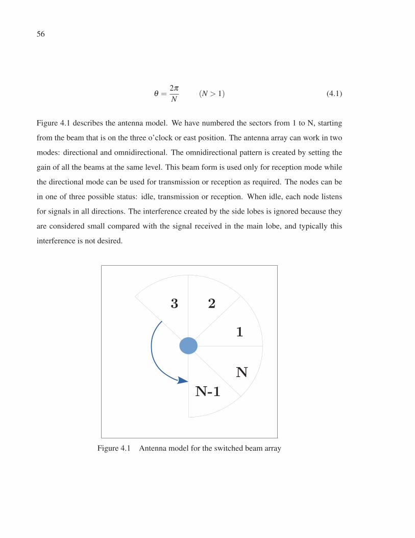
56
θ =2πN
(N > 1) (4.1)
Figure 4.1 describes the antenna model. We have numbered the sectors from 1 to N, starting
from the beam that is on the three o’clock or east position. The antenna array can work in two
modes: directional and omnidirectional. The omnidirectional pattern is created by setting the
gain of all the beams at the same level. This beam form is used only for reception mode while
the directional mode can be used for transmission or reception as required. The nodes can be
in one of three possible status: idle, transmission or reception. When idle, each node listens
for signals in all directions. The interference created by the side lobes is ignored because they
are considered small compared with the signal received in the main lobe, and typically this
interference is not desired.
Figure 4.1 Antenna model for the switched beam array
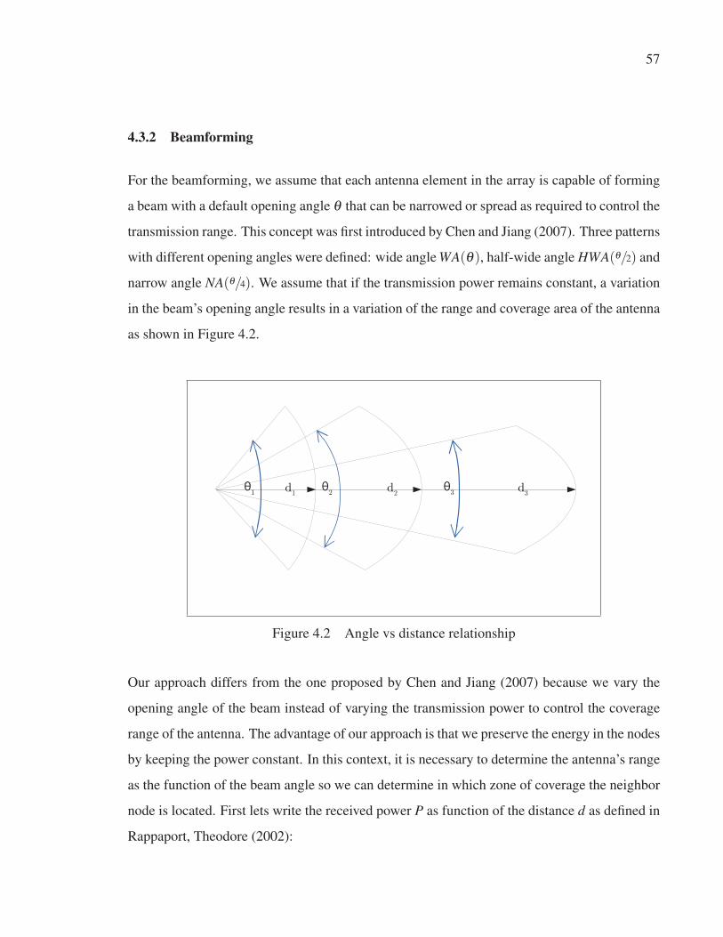
57
4.3.2 Beamforming
For the beamforming, we assume that each antenna element in the array is capable of forming
a beam with a default opening angle θ that can be narrowed or spread as required to control the
transmission range. This concept was first introduced by Chen and Jiang (2007). Three patterns
with different opening angles were defined: wide angle WA(θ), half-wide angle HWA(θ/2) and
narrow angle NA(θ/4). We assume that if the transmission power remains constant, a variation
in the beam’s opening angle results in a variation of the range and coverage area of the antenna
as shown in Figure 4.2.
Figure 4.2 Angle vs distance relationship
Our approach differs from the one proposed by Chen and Jiang (2007) because we vary the
opening angle of the beam instead of varying the transmission power to control the coverage
range of the antenna. The advantage of our approach is that we preserve the energy in the nodes
by keeping the power constant. In this context, it is necessary to determine the antenna’s range
as the function of the beam angle so we can determine in which zone of coverage the neighbor
node is located. First lets write the received power P as function of the distance d as defined in
Rappaport, Theodore (2002):

58
PR(d) =PT GT GRλ 2
(4π)2d2(4.2)
As we consider omnidirectional beamforming at the receiving node in any case, we need to
find the receiving power in the following two cases: the directional-omnidirectional (DO) and
all omnidirectional (OO) connections:
PROO =kPT
dOO2
(4.3)
PRDO =kGT PT
dDO2
(4.4)
Then, we define R as the distance d where the received power is equal to the power threshold
PT H . As we are writing the power equations from the receiver point of view, the threshold
power is always the same for both cases (DO and OO) because we use the directional mode
only for transmissions. Therefore, we equate Equation 4.3 with Equation 4.4 in order to obtain
the relationship between the transmission gain GT and the antenna range d:
PT H = PROO = PRDO
kPT
dOO2=
kGT PT
dDO2
dDO = dOO√
GT (4.5)
Later, we define the distance in omnidirectional mode as the known distance do and we also
define d such as d > do; as the distance in DO mode which is function of d and GT . Then
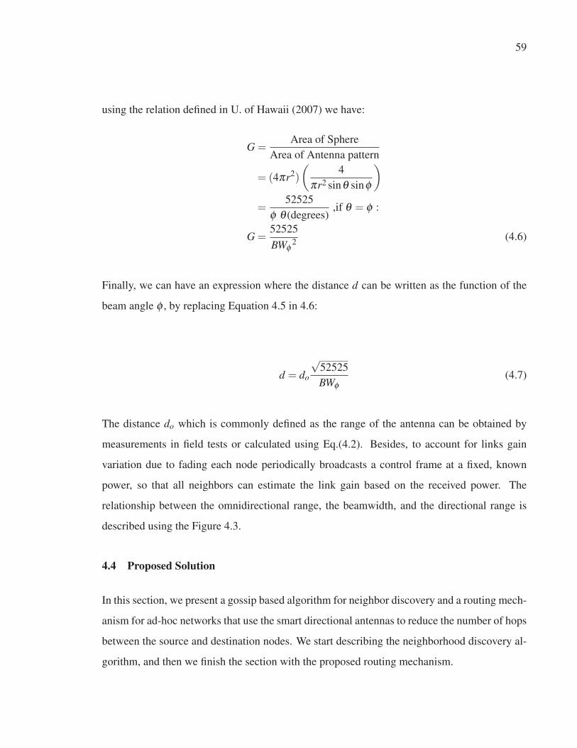
59
using the relation defined in U. of Hawaii (2007) we have:
G =Area of Sphere
Area of Antenna pattern
= (4πr2)
(4
πr2 sinθ sinφ
)
=52525
φ θ (degrees),if θ = φ :
G =52525
BWφ2
(4.6)
Finally, we can have an expression where the distance d can be written as the function of the
beam angle φ , by replacing Equation 4.5 in 4.6:
d = do
√52525
BWφ(4.7)
The distance do which is commonly defined as the range of the antenna can be obtained by
measurements in field tests or calculated using Eq.(4.2). Besides, to account for links gain
variation due to fading each node periodically broadcasts a control frame at a fixed, known
power, so that all neighbors can estimate the link gain based on the received power. The
relationship between the omnidirectional range, the beamwidth, and the directional range is
described using the Figure 4.3.
4.4 Proposed Solution
In this section, we present a gossip based algorithm for neighbor discovery and a routing mech-
anism for ad-hoc networks that use the smart directional antennas to reduce the number of hops
between the source and destination nodes. We start describing the neighborhood discovery al-
gorithm, and then we finish the section with the proposed routing mechanism.

60
Figure 4.3 Omnidirectional vs. directional range
4.4.1 Neighbor discovery
The neighbor discovery algorithm proposed in this paper utilizes a synchronized four-way
handshaking mechanism and assumes that there is a universal timing source that synchronizes
all the nodes in slots over the same timeline. Each time slot is divided into four sub-slots. At
the beginning of each time slot, every node selects a mode between transmission, reception or
idle in the same way as proposed in Liu et al. (2013) with probability pt , pr or pi. If trans-
mission mode is selected in the first sub-slot, the node performs a search using a directional
beam with an angle θ equal to the greatest possible angle that can be formed by the antenna
elements. This fact means that the coverage range is similar to the one that can be achieved
with an omnidirectional beamforming assuming that the power remains constant as proposed
in Equation 4.7.
The search is performed sequentially and following the clockwise direction, and the antenna el-
ement that starts the search is selected at random as shown in Figure 4.4. The unique ID and the
antenna element number used for the transmission is included in the DM before being trans-
mitted. Any node in the surroundings of node i which receives the discovery message(DM)
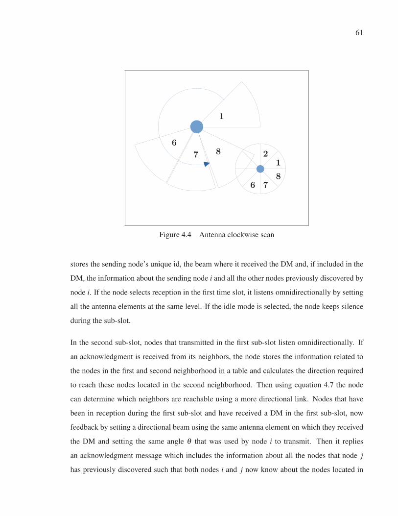
61
Figure 4.4 Antenna clockwise scan
stores the sending node’s unique id, the beam where it received the DM and, if included in the
DM, the information about the sending node i and all the other nodes previously discovered by
node i. If the node selects reception in the first time slot, it listens omnidirectionally by setting
all the antenna elements at the same level. If the idle mode is selected, the node keeps silence
during the sub-slot.
In the second sub-slot, nodes that transmitted in the first sub-slot listen omnidirectionally. If
an acknowledgment is received from its neighbors, the node stores the information related to
the nodes in the first and second neighborhood in a table and calculates the direction required
to reach these nodes located in the second neighborhood. Then using equation 4.7 the node
can determine which neighbors are reachable using a more directional link. Nodes that have
been in reception during the first sub-slot and have received a DM in the first sub-slot, now
feedback by setting a directional beam using the same antenna element on which they received
the DM and setting the same angle θ that was used by node i to transmit. Then it replies
an acknowledgment message which includes the information about all the nodes that node j
has previously discovered such that both nodes i and j now know about the nodes located in

62
the second neighborhood of each other. The node transmits with probability pt and listens
with probability pr. Nodes that have been idle in the first sub-slot remain in silence to avoid
collisions.
In the third sub-slot, nodes that have selected transmission and received an acknowledge in the
second sub-slot will try to reach the nodes in the second neighborhood to confirm that they are
reachable using a more directional beam width. The node sets a directional beam with angle
θ/4 and starts a search on the sectors where there are possible neighboring nodes. Nodes that
have selected reception and has received an advertisement packet in the second sub-slot, now
listen omnidirectionally with pr and keep silence with 1− pr. Nodes in idle mode keep silence
to avoid collisions.
Finally, in the fourth sub-slot nodes in transmission mode listen omnidirectionally. If an ac-
knowledgment is received from the nodes in the second neighborhood, the node marks these
nodes as active. If there is no response from neighbors in the second neighborhood these nodes
are discarded. Nodes in reception mode who have received an advertisement in the third sub-
slot transmits an acknowledgment message with pt and keeps silence with 1− pt . Nodes in
idle mode remain inactive.
4.4.2 Directional Routing
In this section, a novel routing scheme for wireless ad-hoc networks is described. The aim of
this mechanism is to reduce the number of hops in the route between a source and the destina-
tion node using the extended range that can be achieved with smart directional antennas. The
extended range in conjunction with the information about the nodes in the second neighborhood
of a node obtained from the neighbor discovery algorithm proposed previously in this article
are used to reduce the number of hops in a route as illustrated in Figure ??. The algorithm
is intended to be used in a reactive routing protocol such as AODV by Perkins et al. (2003)
or DSR by Johnson and Maltz (1996); where the routes are discovered only when needed. In
this study, we incorporated the developed scheme into AODV, and we named it as directional

63
Algorithm 4.1 4-way handshaking with extended range
1 for each time slot do2 for each node i ∈ N do3 Init: Each node chooses an operating mode: tx, rx or idle, with pt , pr or pi ;
4 In the current slot: Set scan direction as ϕ and scan beamwidth as θ ;
5 end/* In the first sub-slot */
6 if present mode = transmission then7 transmit a discovery message in direction ϕ with beamwidth θ ;
8 else if current mode = reception then listen omnidirectionally;
9 else if current mode = idle then keep silence;
10 end/* In the second sub-slot: */
11 if current mode = transmission then12 listen omnidirectionally;
13 else if current mode = reception then14 transmit NL in the contrary direction of ϕ , with pt or keep silence with 1− pt15 end16 else if current mode = idle then keep silence;
17 end/* In the third sub-slot: */
18 if current mode = transmission then19 transmit a discovery message with direction ψ with BW θ/4;
20 else if current mode = reception then21 If the node has received an discovery message in the second sub-slot, listen
omnidirectionally with pr or keep silence with 1− pr22 end23 else if current mode = idle then keep silence;
24 end/* In the fourth sub-slot: */
25 if current mode = transmission then26 listen omnidirectionally;
27 else if current mode = reception then28 If the node has received a discovery message in the third sub-slot, transmits a
reply message with probability pt or keeps silence with probability 1− pt29 end30 else if current mode = idle then keep silence;
31 end32 end
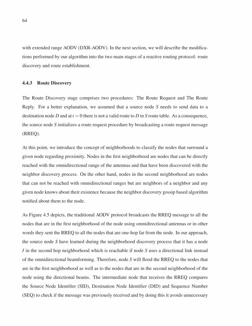
64
with extended range AODV (DXR-AODV). In the next section, we will describe the modifica-
tions performed by our algorithm into the two main stages of a reactive routing protocol: route
discovery and route establishment.
4.4.3 Route Discovery
The Route Discovery stage comprises two procedures: The Route Request and The Route
Reply. For a better explanation, we assumed that a source node S needs to send data to a
destination node D and at t = 0 there is not a valid route to D in S route table. As a consequence,
the source node S initializes a route request procedure by broadcasting a route request message
(RREQ).
At this point, we introduce the concept of neighborhoods to classify the nodes that surround a
given node regarding proximity. Nodes in the first neighborhood are nodes that can be directly
reached with the omnidirectional range of the antennas and that have been discovered with the
neighbor discovery process. On the other hand, nodes in the second neighborhood are nodes
that can not be reached with omnidirectional ranges but are neighbors of a neighbor and any
given node knows about their existence because the neighbor discovery gossip based algorithm
notified about them to the node.
As Figure 4.5 depicts, the traditional AODV protocol broadcasts the RREQ message to all the
nodes that are in the first neighborhood of the node using omnidirectional antennas or in other
words they sent the RREQ to all the nodes that are one-hop far from the node. In our approach,
the source node S have learned during the neighborhood discovery process that it has a node
I in the second hop neighborhood which is reachable if node S uses a directional link instead
of the omnidirectional beamforming. Therefore, node S will flood the RREQ to the nodes that
are in the first neighborhood as well as to the nodes that are in the second neighborhood of the
node using the directional beams. The intermediate node that receives the RREQ compares
the Source Node Identifier (SID), Destination Node Identifier (DID) and Sequence Number
(SEQ) to check if the message was previously received and by doing this it avoids unnecessary

65
loops. Once the RREQ arrives at the destination, the node D initiates a Route Reply procedure
by unicasting a route reply message (RREP). Nodes D and intermediate nodes send the RREP
message using the extended directional links where available, if not, the nodes can always use
the alternative paths as shown in Figure 4.5.
Figure 4.5 Route discovery with omnidirectional antennas
4.4.4 Route Establishment
In the traditional AODV protocol once the source node receives the RREP message the node
S starts to send data to the destination node using the route learned during the route discovery.
As nodes in MANETs are constantly changing their positions, the routes become unstable, and
if a link is broken in the path between source and destination, the route needs to be repaired
or if that is not possible the source node needs to start a Route Request procedure again. In
both cases, the network is flooded with messages that increase the overload traffic and as a
consequence reduces the throughput of the network. To couple with this issue, DXR-AODV
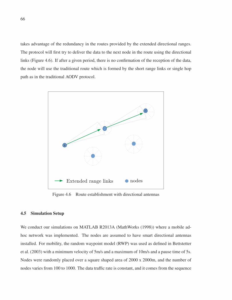
66
takes advantage of the redundancy in the routes provided by the extended directional ranges.
The protocol will first try to deliver the data to the next node in the route using the directional
links (Figure 4.6). If after a given period, there is no confirmation of the reception of the data,
the node will use the traditional route which is formed by the short range links or single hop
path as in the traditional AODV protocol.
Figure 4.6 Route establishment with directional antennas
4.5 Simulation Setup
We conduct our simulations on MATLAB R2013A (MathWorks (1998)) where a mobile ad-
hoc network was implemented. The nodes are assumed to have smart directional antennas
installed. For mobility, the random waypoint model (RWP) was used as defined in Bettstetter
et al. (2003) with a minimum velocity of 5m/s and a maximum of 10m/s and a pause time of 5s.
Nodes were randomly placed over a square shaped area of 2000 x 2000m, and the number of
nodes varies from 100 to 1000. The data traffic rate is constant, and it comes from the sequence

67
of packets delivered for a given source-destination pair in the network. The complete list of
parameters used in the simulations is presented in the Table 4.1.
Table 4.1 Simulations setup
Parameter ValueArea 2000m x 2000m
Number of Nodes 100,200...1000
Mobility Model Random waypoint
Min. velocity 5 m/s
Max. velocity 10 m/s
Pause 5 s
Simulation Duration 3000 s
Packet size 512 bytes
Packet rate 2 pckts/s
Hello interval 1s
Antenna elements (N) 8 per node
Antenna gain 14 dB
Range 200m (omnidirecitonal)
4.6 Results Analysis
In this section, we evaluate the results obtained through the simulation described in section
4.5. The AODV (Perkins et al. (2003)) and LEOD (Quintero et al. (2007)) protocols are used as
performance reference to compare versus DXR-AODV. We evaluated the following parameters:
end-to-end delay, packet loss, and throughput.
4.6.1 Average end to end delay
As it is shown in the figure 4.7 for networks with less than 300 nodes we observed that LEOD
and DXR-AODV perform similarly in terms of average end-to-end delay, while AODV has a
higher end-to-end delay average compared with the directional counterparts of this protocol.
This result is what we were expecting as it has been extensively demonstrated in the litera-
ture that directional antennas can be helpful to reduce the latency in MANETsAlshabtat et al.

68
(2010). Nevertheless, when we compared LEOD versus DXR-AODV we observed that as the
number of nodes is the network reaches the 400 nodes and up our proposed protocol start to
outperform LEOD. We found that the main reason for this is that DXR-AODV is devoted to
reducing the number of hops in a route between source and destination and the reduction in the
number of hops has a direct impact on the end-to-end delay. This result is coherent with the
results that we obtained previously in an analytical model that we developed in Astudillo and
Kadoch (2015)
0
0.2
0.4
0.6
0.8
1
1.2
1.4
100 200 300 400 500 600 700 800 900 1000
Aver
age
end-t
o-en
d d
elay
(s)
N= total number of nodes
AODV
LEOD
DXR-AODV
Figure 4.7 Average end-to-end delay
4.6.2 Packet loss fraction
The packet loss parameter is evaluated as the percentage of packets lost over the total of packets
transmitted. The simulations showed that DRX-AODV outperforms both AODV and LEOD.
This fact can be explained as consequence of two factors. The first reason is that DRX-AODV
offers alternative paths between source and destination because if the extended directional route
is not available, the node can always send the data using the long path as in traditional protocols

69
such as AODV. The second reason is that the number of packet collisions also decreased due
to the improved neighbor discovery algorithm which uses directional links, so increases the
spatial reuse and also implements an idle status in the nodes when they are not transmitting or
receiving which means that these nodes keep silence to avoid collisions.
0
5
10
15
20
25
30
35
100 200 300 400 500 600 700 800 900 1000
Pac
ket
los
s Fra
ctio
n (
PLF)
%
N= total number of nodes
AODV
LEOD
DXR-AODV
Figure 4.8 Packet lost
4.6.3 Throughput
The simulations showed an improvement regarding throughput when DXR-AODV is compared
versus LEOD and AODV. As depicts in Figure 4.9, the three protocols perform similarly when
the number of nodes is not larger than 200 but as the network size increases AODV and LEOD
degrades faster that DXR-AODV. We found that this improvement in the performance is a con-
sequence of two important factors: The first one is related to the directionality in the antennas
by itself because as it was previously demonstrated by Chen et al. (2013) the maximum achiev-
able throughput of ad-hoc networks increases as the angle of the antenna beam decreases. The

70
second factor is related to the redundancy in the routing paths that DXR-AODV offers versus
LEOD and AODV which reduces the demand for repair routes (route repair procedures) or start
the route discovery process again.
70
75
80
85
90
95
100
100 200 300 400 500 600 700 800 900 1000
Tro
ugh
put
(%)
N=total number of nodes
AODV
LEOD
DXR-AODV
Figure 4.9 Throughput
To summarize, in this chapter we presented a novel gossip neighborhood discovery algorithm
that uses the information provided by directional antennas to discover neighbors in the sec-
ond neighborhood of the node using directional beams. Then, a routing algorithm that aims
to reduce the number of hops during the route construction using the information provided by
the neighborhood discovery algorithm also proposed in this chapter and we concluded with
a comprehensive comparison between the scheme suggested in this article and similar solu-
tions previously developed. Nevertheless, the energy consumption was not evaluated in this
chapter, and it can be a good future work to determine the improvements in terms of energy
consumption that can be achieved when directional antennas are used in ad-hoc networks.

CHAPTER 5
ENERGY MODEL FOR DIRECTIONAL AD-HOC NETWORKS
5.1 Introduction
As mentioned in previous chapters, ad-hoc networks have an important set of applications in
industry, military, personal, sensors and vehicular networks. No matter if the nodes are moving
or not, most of this applications require nodes to be powered by batteries or solar panels which
are a limited source of energy. Therefore, researchers in the past have given a lot of attention
in ad-hoc protocols that consider efficient algorithms to reduce the energy consumption. In the
literature review, we identified two methods as the most used ones to evaluate the performance
of these protocols: simulation using an appropriate software or through a mathematical model
using graph theory. Although both methods have been proven to be efficient, we will focus on
the graph theoretical model to give continuity to our work and also because we have identified
that there is a lack of consideration of the directionality on the models developed so far. To
accomplish this aim, in this chapter we present an overview of the relevant research works
done so far, then we introduce a novel model for estimating the energy consumed in MANETs
when smart directional antennas are installed on the nodes. Subsequently, we describe the
setup assumptions for the model validation, and we finalize the chapter with an analysis of the
obtained results and some proposals for future work.
5.2 Proposed Model
This model is based on the model that we have previously developed in Section 3.3. We depart
from the same assumption that at any time a wireless ad-hoc network can be represented as a
graph G(V,E) where the vertices represent the nodes and the edges represent the energy used
to transmit information from one node to other. To estimate the energy consumed, we first
will need to determine the connectivity between nodes using the model proposed in section.
Then, we construct the graph with all the possible routes between one source node and all other

72
nodes. After that, the shortest path between source and destination must be determined. Once
the paths from all nodes to the given node are calculated, the number of messages transmitted
during the session can be determined. Finally, with the number of messages transmitted, the
consumed energy can be estimated. In the following sections, we will describe in detail our
model.
5.2.1 Node Distribution Model
As in Chapter 3, we consider that nodes are uniformly distributed over a square shaped service
area of length M; therefore, the coverage area is defined as Ω = M×M and the node density is
defined as d = NΩ where N is the total number of nodes.
5.2.2 Network Topology
In real scenarios nodes are positioned on a three dimensional space (xi,yi,zi) but in order to
simplify our analysis and following a commonly accepted assumption made in several previous
works, we have decided to use a two dimensional array (xi,yi) with N columns where N is equal
to the number of nodes in the network. The network topology of the area to be studied is then
represented as shown on Table 5.1
Table 5.1 Position of the nodes array
ID 1 2 3 ... NX pos x1 x2 x3 ... xNY pos y1 y2 y3 ... yN
5.2.3 Antenna model
In general terms, an antenna is a device that is capable to radiate or collect radio signals in all
directions(omnidirectional case) or in a specific direction(directional case). Traditional wire-
less networks are equipped with omnidirectional antennas but recently the research community
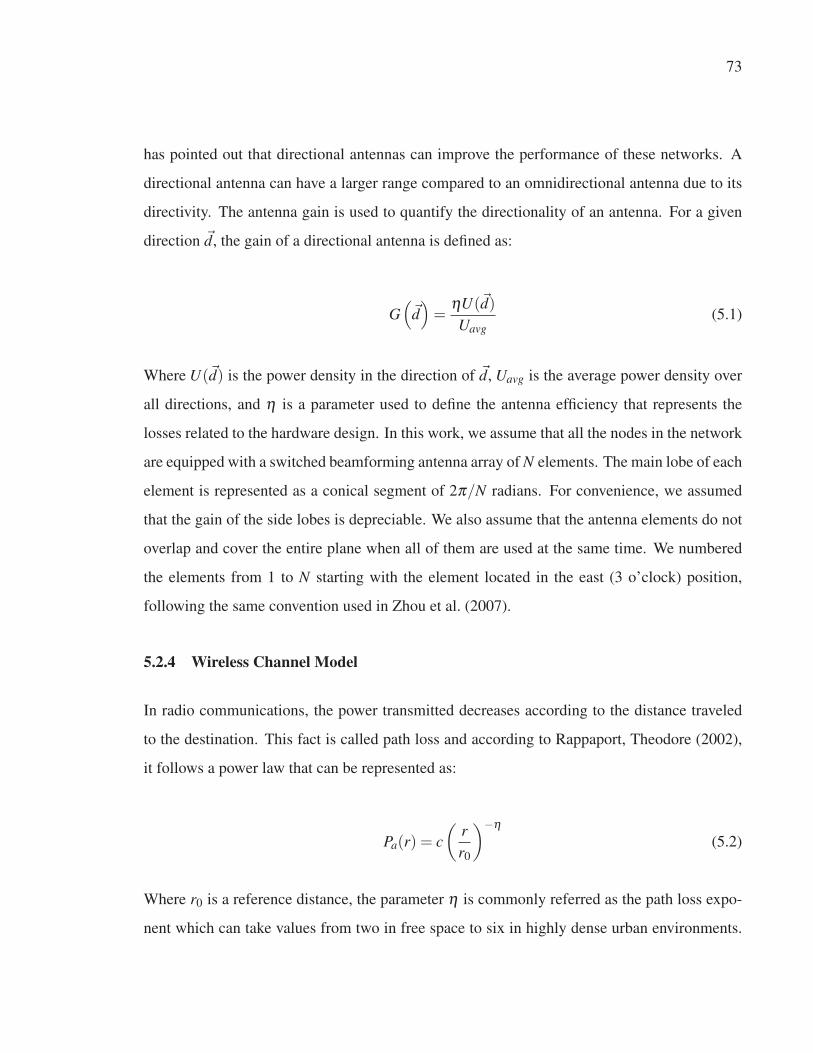
73
has pointed out that directional antennas can improve the performance of these networks. A
directional antenna can have a larger range compared to an omnidirectional antenna due to its
directivity. The antenna gain is used to quantify the directionality of an antenna. For a given
direction �d, the gain of a directional antenna is defined as:
G(�d)=
ηU(�d)Uavg
(5.1)
Where U(�d) is the power density in the direction of �d, Uavg is the average power density over
all directions, and η is a parameter used to define the antenna efficiency that represents the
losses related to the hardware design. In this work, we assume that all the nodes in the network
are equipped with a switched beamforming antenna array of N elements. The main lobe of each
element is represented as a conical segment of 2π/N radians. For convenience, we assumed
that the gain of the side lobes is depreciable. We also assume that the antenna elements do not
overlap and cover the entire plane when all of them are used at the same time. We numbered
the elements from 1 to N starting with the element located in the east (3 o’clock) position,
following the same convention used in Zhou et al. (2007).
5.2.4 Wireless Channel Model
In radio communications, the power transmitted decreases according to the distance traveled
to the destination. This fact is called path loss and according to Rappaport, Theodore (2002),
it follows a power law that can be represented as:
Pa(r) = c(
rr0
)−η(5.2)
Where r0 is a reference distance, the parameter η is commonly referred as the path loss expo-
nent which can take values from two in free space to six in highly dense urban environments.
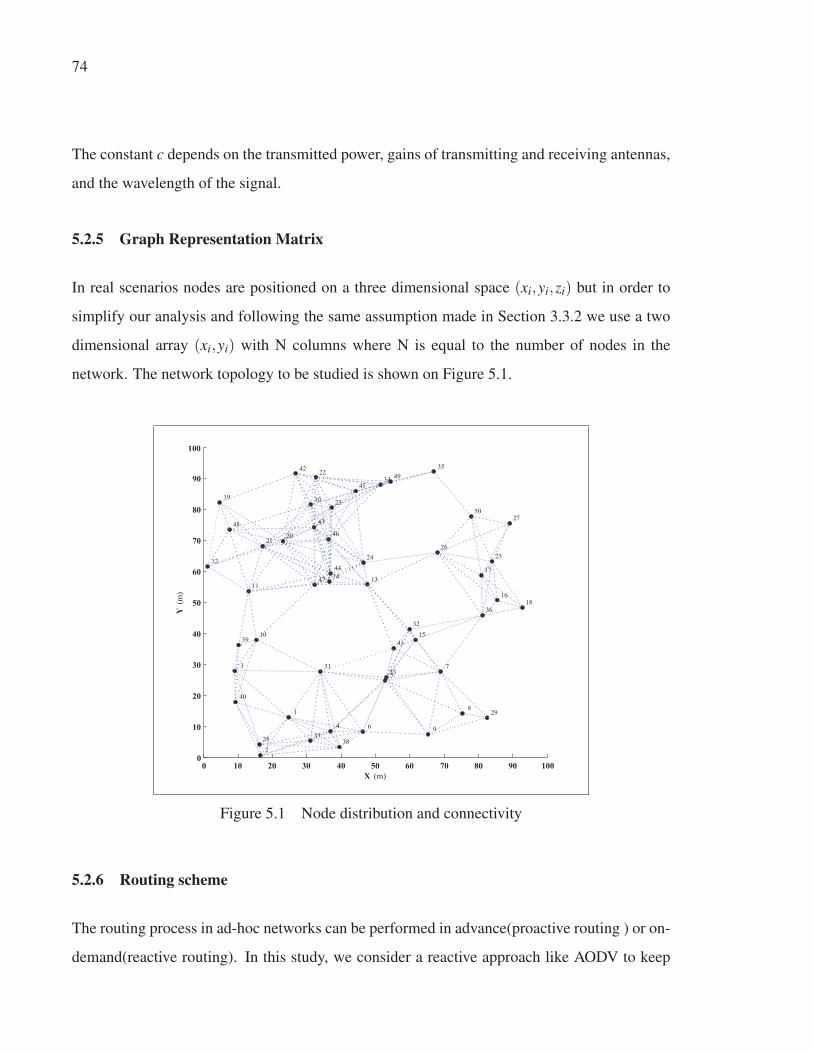
74
The constant c depends on the transmitted power, gains of transmitting and receiving antennas,
and the wavelength of the signal.
5.2.5 Graph Representation Matrix
In real scenarios nodes are positioned on a three dimensional space (xi,yi,zi) but in order to
simplify our analysis and following the same assumption made in Section 3.3.2 we use a two
dimensional array (xi,yi) with N columns where N is equal to the number of nodes in the
network. The network topology to be studied is shown on Figure 5.1.
0 10 20 30 40 50 60 70 80 90 1000
10
20
30
40
50
60
70
80
90
100
X (m)
Y (m
)
1
2
3
4
5
6
7
8
9
10
11
12
1314
15
16
17
18
19
2021
22
23
24 2526
27
28
29
30
31
32
33
34
35
36
3738
39
40
41
42
43
44
45
46
47
48
49
50
Figure 5.1 Node distribution and connectivity
5.2.6 Routing scheme
The routing process in ad-hoc networks can be performed in advance(proactive routing ) or on-
demand(reactive routing). In this study, we consider a reactive approach like AODV to keep

75
coherence with the first stages of this thesis. In a reactive scheme, the route is calculated step
by step and the next hop of the route is selected considering a given or desired parameter such
as hop count, link quality, residual energy among others. Therefore, the route with less cost
in terms of the desired parameter is chosen as the best route. For this reason, the shortest path
algorithm is commonly used in this mechanisms. From the literature review, we observed that
the Dijkstra algorithm is the most used approach which is a single-source shortest path algo-
rithm. However, the weight of all the edges must be non-negative or in other words, Dijkstra is
not able to detect loops in the route. As we experienced loop issues during the simulations in
the first stage of our research, we investigated the alternatives to Dijkstra and we found that the
Bellman-Ford algorithm is also a single-source shortest path algorithm, similar to Dijkstra but
it allows for negative edge weights and it can detect loops in a graph. The Bellman-Ford algo-
rithm is implemented into the graphshortestpath function that comes in the Network Analysis
and Visualization class of the Bioinformatics toolbox of MATLAB(MathWorks (2012)):
[distSP, path, pred] = graphshortest path(G,S,D,method,Bellman−Ford)
The graphshortest path function determines the single-source shortest paths from nodes S to D
in the graph represented by matrix G. As inputs, this function requires G which is an N-by-N
sparse matrix that represents a graph. Nonzero entries in matrix G represent the weights of the
edges. distSP are the N distances from the source to the destination node. pat contains the
winning path. pred contains the predecessor nodes of the winning path. Figure 5.2 shows a
sequence (from a to d) of messages sent from node 25 to every other node in the network and
the corresponding routing path established (nodes 5 to 8 in the example).
The matrix G is constructed based on the network topology array in the following way: Using
the function described in algorithm 3.1, we go over the array which represents the network.
On each iteration, the Euclidean distance between each pair of nodes is calculated. Then, this
distance is normalized and the connection between any two nodes is determined based on the
directional link probability. If p(ri j
)=Pr
[10log10P
(ri j
)> 0
]a link between i and j is drawn.

76
a) First iteration b) Second iteration
c) Third iteration d) Fourth iteration
Figure 5.2 Several iterations from node 25
5.3 Energy Cost of Communication
Once the paths from the source node (number 25 in the example) to every other node in the
network are calculated, the number of messages exchanged during the communication can be
estimated. To illustrate this fact, let’s consider the set of five nodes in Figure 5.3 where node n1
starts the route discovery and tries to deliver a message to n5. In this case, we have one source
node, one destination node, and three intermediate nodes.

77
Figure 5.3 Unicast cost with omnidirectional antennas
5.3.1 Omnidirectional Energy Cost
Let’s first consider that all the nodes only have omnidirectional antennas. Node 1 propagates
a message so node 2 receives the message, checks the routing header and checks the cyclic
redundancy (CRC) and then sends the message downstream but due to the omnidirectional
nature of the network, node 1 receives back from node 2 a copy of the propagated message with
a different destination address. As it does not correspond to it, the message is discarded but it
was overhead by n1. This fact is called the overhead message and it was widely investigated
by Basu and Redi (2004).
For the simulation, we considered a store-and-forward procedure where every message is re-
ceived then read it. If the message is destined for the given node it is processed otherwise it
is discarded. This last statement means that even if a message is not destined to a given node,
the node uses energy to receive and process the message. For simplicity, we also assume that

78
the energy consumed by the overhead EOH is equal to the energy required for reception ERX .
Therefore the node that starts the route discovery n1 consumes E1.
E1 = ET X +EOH
E1 = ET X +ERX (5.3)
The intermediate nodes consumes ERX when receiving the forwarded message plus the energy
required for re-transmit the message downstream ET X , finally they overhead the message sent
back by the downstream node so they consumes in addition EOH . Hence, the energy consumed
by relaying nodes Erel is:
Erel = ET X +ERX +EOH
= ET X +2ERX (5.4)
The next aspect to consider is the energy consumed by broadcasting. In terms of reactive
protocols such as AODV, this energy is a representation of the messages used to discover the
neighbor nodes of a given node. The effect of HELLO messages in AODV was studied in
Bhanushali et al. (2015) while the energy consumed by broadcasting in ad-hoc networks was
extensively modeled by Wieselthier et al. (2000).
From this last research work, we adopt the Wireless Multicast Advantage (WMA) model.
WMA is used to describe the energy cost of the rebroadcasted message, and to illustrate this
fact we use the Figure 5.3. In the figure, Ni broadcast a message that is heard by all the neigh-
bor nodes in the range of Ni. Consequently, all the nodes within the range of Ni will respond
to the broadcast message and Ni spent energy listening to the responses. Thus, we can state
that the energy cost of the broadcasted message is affected by the presence of the neighbors

79
of the broadcasting node. This means that for every message that node i receives and rebroad-
cast it consumes ET X +ERX plus the energy required to overhear the acknowledgment from its
neighbors. Therefore, the total energy consumed is given by equation 5.5:
Ei = ERX +ET X +(mi −1)ERX (5.5)
Where (mi−1) represents the fact that the message broadcasted is overhead by node i from all
the nodes m∈Mi that surround the node except the node that sends the broadcast message. This
model was used in many relevant works such as Singh and Raghavendra (1998) and Wieselthier
et al. (2000).
Finally, to calculate the cost of the messages transmitted during the communication process, it
is necessary to count the messages transmitted, received and overhead. This is performed on
each iteration during the simulation time. As it was proposed by Wieselthier et al. (2000), we
use the matrix TxRxOx to count the messages as it is shown in table 5.2.
Table 5.2 Number of messages matrix
ID 1 2 3 ... NRx 8 23 48 ... 73
Tx 2 36 53 ... 42
Ox 12 4 2 ... 26
Total 22 63 103 ... 141
5.3.2 Proposed Solution: Directional Energy Cost
In the past section, we presented an energy cost model developed by previous researchers that
consider omnidirectional transmissions. In order to contribute to this important field of the
telecommunications industry, we propose to consider directional transmissions in the energy
cost model for ad-hoc networks. To illustrate our model, consider the Figure 5.4, where the

80
node n1 initiates a route discovery to deliver a message to n5. Assuming that the nodes im-
plement the neighbor discovery protocol that we previously developed in Section 4.2.1, it is
possible for n1 and n3 to reduce the number of hops by knowing that they can reach n3 and n5
respectively using directional links instead of omnidirectional beamforming.
To reach these further nodes, our model does not consider to increase the power of the trans-
mitters, therefore the energy required for transmitting remains as constant and equal to ET X ,
The energy used for reception in our model is the same as in the omnidirectional case because
we have assumed omnidirectional reception in any case.
Figure 5.4 Unicast cost with directional antennas
Therefore the node that starts the route discovery (n1) consumes E1:
E1 = ET X +ERX (5.6)

81
Then, the intermediate node or relay node consumes energy when receiving the route discovery
message(ERX ), then it retransmits the message downstream but instead of transmitting it om-
nidirectionally, intermediate nodes transmits directionally to the next hop. If the node knows
about distant nodes that can be reached using longer beams, the node will try to reach them. As
we assume that distant nodes can be reached by narrowing the beams instead of increasing the
transmission power, the Energy used for transmissions is constant and equal to ET X . Hence,
the energy consumed to move downstream a message is as presented in Equation 5.7:
Erel = ET X +ERX (5.7)
For the broadcasting cost, we assume that the node sends the broadcast messages omnidirec-
tionally by setting the antenna elements heights to the same value so the energy consumed is
equivalent to the omnidirectional case as is presented in Equation 5.8:
Ei = ERX +ET X +(mi −1)ERX (5.8)
Finally, we calculate the total cost of communication by adding the cost of unicasted and
broadcasted messages:
Eunicast = Eunicast +Ebroadcast (5.9)
Where the energy consumed when unicasting is:
Eunicast = E1 +Mi
∑n=1
Erel +Edest (5.10)

82
and the energy consumed when broadcasting is:
Ebroadcast = ∑Ei
= ET X +miERX (5.11)
Counting the number of messages transmitted, received and overheard can be performed dur-
ing the path discovery processes. In our implementation, we count the messages transmitted,
received and overhead using the RxTxOx matrix (see Table 5.2). On each iteration, the number
of messages is counted and then saved on the matrix. Once the paths are established and the
number of messages is counted, we proceed to calculate the total energy consumed as we detail
in the next section.
5.4 Energy model for messages transmitted
In this section, we propose an energy model that estimates the energy consumed by an ad-
hoc wireless network. We based our model on the assumption that the total energy that every
node spend is directly proportional to the time that each node stays in sleep, idle, transmission
and reception mode. This assumption was also used in previous models, such as Simek and
Moravek (2011).
The first step during the modeling process was to study the IEEE 802.11 specification (IEEE
(2012)) and determine the time required for every process that leads to a successful message
transmission. Then, the energy consumption of the communication modes can be obtained
from the chipset data sheets. For our model, we searched for a widely used transceiver chip. We
use the information of the Microchip MRF24GWG0MA RF transceiver (Microchip (2016)).
According to the data sheet, it consumes 0.1 mA in sleep mode, 4 mA in idle mode, 156 mA
when receiving and 240 mA when transmitting. Finally, with the information obtained in the
previous steps and assuming the successful transmission of a data packet, the energy consumed
per message transmitted, received and overheard can be estimated.
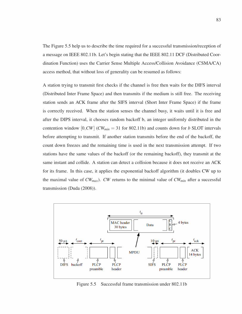
83
The Figure 5.5 help us to describe the time required for a successful transmission/reception of
a message on IEEE 802.11b. Let’s begin stating that the IEEE 802.11 DCF (Distributed Coor-
dination Function) uses the Carrier Sense Multiple Access/Collision Avoidance (CSMA/CA)
access method, that without loss of generality can be resumed as follows:
A station trying to transmit first checks if the channel is free then waits for the DIFS interval
(Distributed Inter Frame Space) and then transmits if the medium is still free. The receiving
station sends an ACK frame after the SIFS interval (Short Inter Frame Space) if the frame
is correctly received. When the station senses the channel busy, it waits until it is free and
after the DIPS interval, it chooses random backoff b, an integer uniformly distributed in the
contention window [0,CW ] (CWmin = 31 for 802.11b) and counts down for b SLOT intervals
before attempting to transmit. If another station transmits before the end of the backoff, the
count down freezes and the remaining time is used in the next transmission attempt. If two
stations have the same values of the backoff (or the remaining backoff), they transmit at the
same instant and collide. A station can detect a collision because it does not receive an ACK
for its frame. In this case, it applies the exponential backoff algorithm (it doubles CW up to
the maximal value of CWmax). CW returns to the minimal value of CWmin after a successful
transmission (Duda (2008)).
Figure 5.5 Successful frame transmission under 802.11b

84
Therefore, to estimate the total time required for a successful transmission we use the informa-
tion about the time needed for each interval that we obtained from the IEEE 802.11 specifica-
tion. This information is resumed in the table 5.3.
Table 5.3 IEEE 802.11 MAC and PHY parameters
variant bit rate (Mb/s) DIFS SIFS SLOT tpr μs802.11b 1, 2, 5.5, 11 28 μs 10 μs 20 μs 192, 96
802.11g 6, 9, 18, 24, 28, 36, 48, 54 28 μs 10 μs 9 μs 22.1
To calculate the total time required to successfully transmit a message we made some assump-
tions and follow the sequence described below:
• The nodes communicate with each other using the TCP protocol;
• Assume that each TCP data packet is followed by a TCP ACK packet;
• To transfer the data segment there will be silence during at least one DIFS slot, signaling
that the medium is available. More than one if the node is executing back-off;
• The data frame containing the TCP data;
• A SIFS gap between data frame and 802.11 ACK frame;
• The 802.11 ACK frame.
Then, to transfer the TCP ACK packet:
• There will be a silence during at least one DIFS slot, signaling that the medium is available.
More than one if the node is executing back-off;
• The data frame containing the TCP ACK;
• A SIFS gap between data frame and 802.11 ACK frame;

85
• A 802.11 ACK frame
In addition to the payload data, the data frame has additional 36 bytes of data, out of those 28
bytes are 802.11 MAC header for various inherent functions such as control and management,
error detection and addressing. The other 8 bytes are a header to identify the network layer
protocol.
To transfer 1460 bytes of payload in 802.11b at 11 Mb/s, we have a packet with 1500 bytes of
data including the TCP/IP headers, and 1536 bytes if we consider the MAC header. For the
TCP ACK packet of 40 bytes there is also an additional 36 bytes for MAC header, so total 76
bytes for the TCP ACK.
The 802.11 ACK frame has a length of 14 bytes. We neglect media contention and retransmis-
sions. At 11 Mb/s the data rate is 1.375 Msymbols/s, where each symbol is 8 bits. Thus the
time required to transmit a data packet can be calculated by the equation:
tT X = DIFS+ tpr + ttr +SIFS+ tpr + tACK (5.12)
= 50μs+192μs+1536/1.375+10μs+192μs+14/1375
= 1573μs
In the same way, the time required to transmit a TCP ACK packet can be estimated. In this
case, the ttr is calculated using the size of the TCP ACK message (76 bytes), as we present
here. In total we need 2084 μs to transmit 1460 bytes of payload:
tACK = DIFS+ tpr + ttr +SIFS+ tpr + tACK (5.13)
= 50μs+192μs+76/1.375+10μs+192μs+14/1375
= 511μs

86
Following the same procedure present before, we can calculate the time needed to receive a
message:
tRX = DIFS+ tpr + ttr +2×SIFS+ tACK (5.14)
= 50μs+192μs+1536/1.375+20μs+14/1375
= 1389μs
Once the time spent in both active status (transmission and reception) is determined, we can
estimate the energy consumed per node on each computed route to the destination. To do so,
we need the voltage and current that the chipset uses on each status, table 5.4 presents this
information. As illustration, we calculate the energy dissipated by the sender node, (n1 in
Figure 5.4):
E1 =V × I × t (5.15)
= 3.3[V ]×240[mA]×1.5[ms]
= 1.18[mJ]
In the same way, the energy dissipated for every node in the route can be calculated. For a
more precise result, the power can be measured in real devices, in this research work we just
presented a simplified calculation.
Table 5.4 MRF24WG0MA/MB Parameters
Mode Current VoltageRX 156 mA (typical) 3.3 V (typical)
TX 240 mA (typical) 3.3 V (typical)
Idle 4 mA (typical) 3.3 V (typical)
Sleep 0.1 mA (typical) 3.3 V (typical)
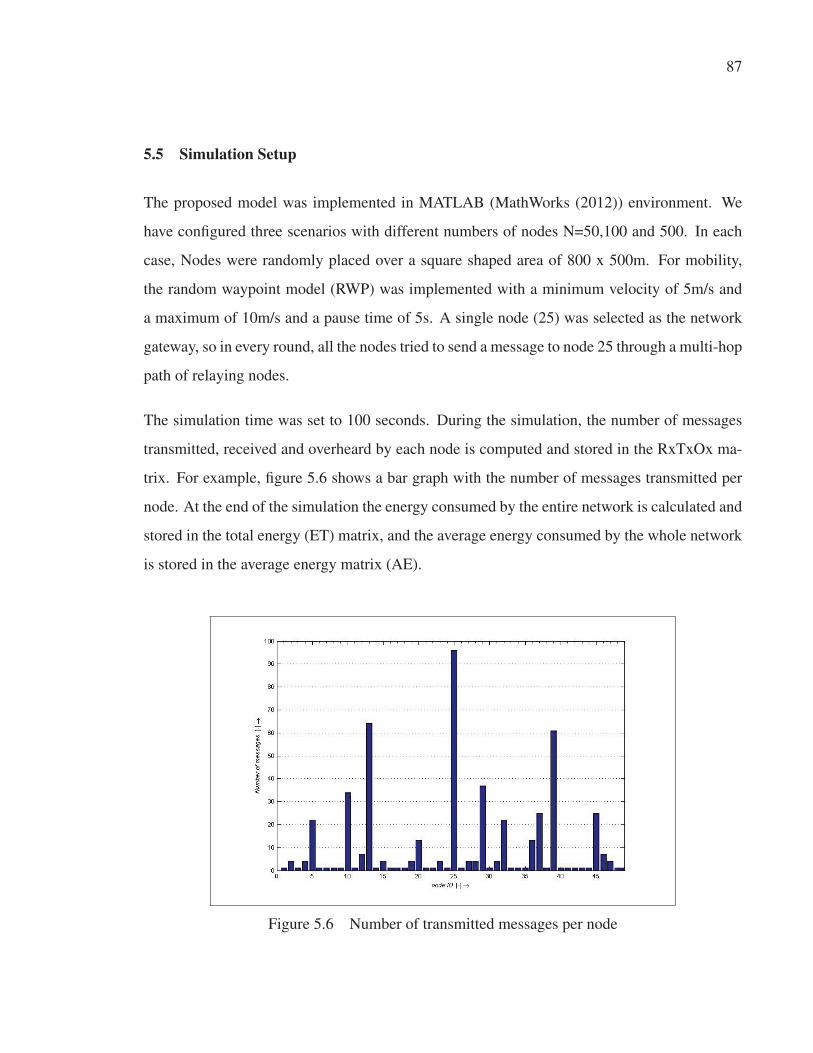
87
5.5 Simulation Setup
The proposed model was implemented in MATLAB (MathWorks (2012)) environment. We
have configured three scenarios with different numbers of nodes N=50,100 and 500. In each
case, Nodes were randomly placed over a square shaped area of 800 x 500m. For mobility,
the random waypoint model (RWP) was implemented with a minimum velocity of 5m/s and
a maximum of 10m/s and a pause time of 5s. A single node (25) was selected as the network
gateway, so in every round, all the nodes tried to send a message to node 25 through a multi-hop
path of relaying nodes.
The simulation time was set to 100 seconds. During the simulation, the number of messages
transmitted, received and overheard by each node is computed and stored in the RxTxOx ma-
trix. For example, figure 5.6 shows a bar graph with the number of messages transmitted per
node. At the end of the simulation the energy consumed by the entire network is calculated and
stored in the total energy (ET) matrix, and the average energy consumed by the whole network
is stored in the average energy matrix (AE).
Figure 5.6 Number of transmitted messages per node

88
5.6 Results Analysis
In this section, we present the results obtained through the simulation described in section 5.5.
The first scenario was setup with 50 nodes uniformly distributed in a 500m×800m area, we run
the same script 100 times, and we take the average. Figure 5.7 shows the total energy consumed
by the ad-hoc network when omnidirectional antennas (blue line) and directional antennas
(orange line) are used. Red and green dotted lines represent the average energy consumed
in each case respectively. As we can see in figure 5.7, the average energy consumed by the
50 nodes network when using directional antennas is 35% more efficient than when using
omnidirectional antennas.
50
100
150
200
250
300
350
400
450
500
1 10 19 28 37 46 55 64 73 82 91 100
Ener
gy [m
J]
Simulation time [s]
DXR-AODV AODV
Figure 5.7 Total Energy Consumed: 50 Nodes scenario
Figures 5.8 shows the results obtained when the number of the antennas increases to 100 and
nodes assuming the same coverage area as in the previous experiment (500m×800m). In this
case, we observed that the average energy consumed by the network when using directional
antennas is 18% more efficient than when using omnidirectional antennas. Although there is
still an improvement in the energy consumption, we observed that this contribution is lower
than the case with just 50 nodes. This fact is a consequence of the increased network density

89
because of the more the nodes in the network, the higher the total amount of traffic each node
generates.
400
500
600
700
800
900
1000
1100
1 10 19 28 37 46 55 64 73 82 91 100
Ener
gy [m
J]
Simulation time [s]
DRX-AODV AODV
Figure 5.8 Total Energy Consumed: 100 Nodes scenario
Consequently, more traffic is going over the network per time unit and energy is depleted more
quickly. This is a critical remark because the energy saving that a protocol can contribute to
saving can not be infinite and as was previously demonstrated by the fundamental research
done by Spyropoulos and Raghavendra (2002) there is a boundary in the energy that can be
saved with directional antennas in ad-hoc networks.
As consequence of the results of the last experiment, we wanted to determine the number of
nodes where both solutions (directional and omnidirectional) perform similarly. We define a
scenario with 500 nodes uniformly distributed in a 500m×800m area, we run the same script
100 times, and we take the average. Figure 5.9 shows the results of this simulation. We can
observe that the average energy consumed by the network when using directional antennas is
just 1.25% more efficient than when using omnidirectional antennas. We considered that at this

90
point both methods work equally so for more than 500 nodes there is no difference regarding
energy consumption to use any of them.
3.2
3.7
4.2
4.7
5.2
5.7
6.2
6.7
7.2
7.7
1 10 19 28 37 46 55 64 73 82 91 100
Ener
gy [J
]
Simulation time [s]
DRX-AODV AODV
Figure 5.9 Total Energy Consumed: 500 Nodes scenario
To summarize, in this chapter we presented an energy model based on graph theory that con-
siders the energy dissipated by smart directional antennas. We have demonstrated that there
are important reductions in the energy consumed in ad-hoc networks when using directional
antennas that in the best case can save up to 35% of the total energy. Nevertheless, we conclude
that as the number of the nodes increases from 50 to 500 the improvement in energy savings as
consequence of the use of directional antennas experience a reduction.
Although our proposed solution performs better that AODV when the number of nodes is
relatively smaller, we noticed a decrease in the energy that can be saved when using directional
antennas as the number of the nodes increases. This event can be explained as consequence of
the increased node density in the network. Even if we are reducing the path lengths between
nodes, the fact that there are more nodes in the network implies more traffic to be generated.
The more the nodes in the network, the higher the total amount of traffic each node generates.
Consequently, more traffic is going over the network per time unit and energy is depleted more
quickly.

CONCLUSION AND RECOMMENDATIONS
The use of smart directional antennas in ad-hoc wireless networks has been an active research
topic in the last decade. Most of the previous work has been focused on adapting the existing
MAC protocols to support directional antennas or make an efficient spectral reuse to obtain a
higher feasible bandwidth. In this thesis, we investigated the impact of directional antennas in
the neighbor discovery process and the routing protocols concerning network performance as
well as energy consumption.
This research work first developed a model for wireless ad-hoc networks with directional an-
tennas using a graph theoretical approach. We proposed an innovative link probability model
that considers the directional gain of the smart antenna array. Through simulations, we demon-
strated that it is possible to achieve a higher network connectivity when directional antennas
are considered in the model. We also observed that as the main lobe of the antenna array is
narrowed and consequently the antenna range is extended, the probability to have a link with
nodes that are farthest is higher if it is compared to the omnidirectional model.
Hop count is an important metric in wireless ad-hoc networks because every hop in the route
implies an increase in the delay between source and destination due to message processing
on the relaying nodes, propagation, and signaling. Regarding the hop count, we have also
noticed a reduction in the mean hop count when the directional model is used. Fewer hops in
any path between a source and destination node are considered as an improvement in network
performance because of more hops in a route necessary lead to a higher transmission delay.
This thesis also studied the neighborhood discovery and routing protocol issues in wireless
ad-hoc networks when smart directional antennas are included in the system. The aim at this
stage of the thesis was to reduce the number of hops between source and destination nodes. As
a solution, we have proposed DXR-AODV protocol which is an enhancement of the traditional
AODV protocol. From the simulations performed in this research work, we concluded that our

92
scheme outperforms AODV and LEOD protocols concerning end-to-end delay, throughput,
and packet loss when they are compared in the scenarios described in this thesis.
The energy consumption was also evaluated in this thesis. We analyzed the impact of the
reduction in the number of hops in a route in terms of the energy consumed by the entire
network. To do this analysis, it was necessary to model the relationship between the use of
the extended range antenna and the power consumption. Through simulations, we have proved
that in the best scenario, directional antennas can provide up to 35% of energy savings when
compared to omnidirectional antennas.
Future Work
This research work addressed the impact of smart directional antennas in ad-hoc networks
taking into account the improvements regarding performance and energy consumption that can
be achieved in the neighborhood discovery and routing schemes when the smart antennas are
used. Some perspectives for the continuation of this thesis are listed below:
• This thesis assumed some ideal conditions to reduce the complexity of the analysis. For
example, the main lobe of the antennas was assumed as a conical shape projected over
the X-Y plane and that the side lobes do not interfere with the main lobe of the antenna.
It will be interesting to consider a three-dimensional model as well as the interference of
the sidelobes to analyze the impact of these two factors in the performance and energy
consumption of the ad-hoc network;
• During the development of this thesis a fundamental, pure ad-hoc network was assumed
in the models. It will also be interesting to apply the results of this work to a particular
application or scenario such as a Disaster Recovery network, Military or Public Security
Network;

93
• Finally, the models proposed in this thesis were evaluated over a simulated environment
which is a good representation of the reality, but we consider that it will be interesting to run
the solutions proposed in a real scenario such as a testbed with real nodes and antennas. As
an example, we can cite the Project IoT-Lab (European Comission, 2016) where a network
with real mobile sensors can be used to test innovative developments in the ad-hoc, IoT and
sensors networks.


APPENDIX I
LIST OF PUBLICATIONS
Journals:
J-1 Astudillo, G. & Kadoch, M. 2016. Neighbor discovery and routing schemes for mobile ad-
hoc networks with beamwidth adaptive smart antennas. Telecommunication Systems,
4, 5280-5292, Springer Verlag. doi: 10.1007/s11235-016-0268-x.
J-2 Astudillo, G. & Kadoch, M. 2017. A Realistic Energy Model for Wireless Ad-hoc Net-
works with Smart Directional Antennas. Article summited to Ad-Hoc Networks, Else-
vier.
Conferences:
C-1 Astudillo, G. & Kadoch, M. 2014. A Location-aware Routing Scheme for Wireless Mesh
Networks using Directional Antennas. Recent Advances in Computer Engineering,Communications and Information Technology, 1, 57-62.
C-2 Astudillo, G. & Kadoch, M. 2015. Impact of Directional Antennas on Link Probability
and Connectivity in Wireless Ad-Hoc Networks. 2015 3rd International Conferenceon Future Internet of Things and Cloud, 1, 218-224. doi: 10.1109/FiCloud.2015.60.


BIBLIOGRAPHY
Abolhasan, M., T. Wysocki, and E. Dutkiewicz. 2004. "A review of routing protocols for
mobile ad hoc networks". Ad Hoc Networks 2(1), 1–22.
Almeida, N., M. Fernandes, and A. Neto. 2015. "Beamforming and Power Control in Sensor
Arrays Using Reinforcement Learning". Sensors 15(3), 6668–6687.
Alshabtat, A., L. Dong, J. Li, and F. Yang. 2010. "Low latency routing algorithm for unmanned
aerial vehicles ad-hoc networks". International Journal of Electrical, Computer, Ener-getic, Electronic and Communication Engineering 6(1), 48–54.
An, X. and R. Hekmat. 2007. "Self-Adaptive Neighbor Discovery in Ad Hoc Networks with
Directional Antennas". In 2007 16th IST Mobile and Wireless Communications Summit,pp. 1–5. IEEE.
Anastasi, G., M. Conti, and E. G. Laurea. 2005. "IEEE 802.11 Ad Hoc Networks: Protocols,
Performance and Open Issues". Mobile Ad Hoc Networking 1(1), 69–116.
Aschner, R., M. J. Katz, and G. Morgenstern. 2013. "Symmetric connectivity with directional
antennas". Computational Geometry: Theory and Applications 46(9), 1017–1026.
Astudillo, G. and M. Kadoch. 2015. "Impact of Directional Antennas on Link Probability and
Connectivity in Wireless Ad-Hoc Networks". In 2015 3rd International Conference onFuture Internet of Things and Cloud, pp. 218–224. IEEE.
Astudillo, G. and M. Kadoch. 2017. "Neighbor discovery and routing schemes for mobile
ad-hoc networks with beamwidth adaptive smart antennas". Telecommunication Sys-tems 1(1), 1–11.
Basagni, S., I. Chlamtac, V. R. Syrotiuk, and B. a. Woodward. 1998. "A distance routing
effect algorithm for mobility (DREAM)". In Proceedings of the 4th annual ACMIEEEinternational conference on Mobile computing and networking MobiCom 98, pp. 76–84.
IEEE.
Basu, P. and J. Redi. 2004. "Effect of overhearing transmissions on energy efficiency in dense
sensor networks". In Proceedings of the third international symposium on Informationprocessing in sensor networks - IPSN’04, New York, New York, USA, pp. 196–202.
ACM Press.
Bettstetter, C.. 2002. "On the Minimum Node Degree and Connectivity of a Wireless Multihop
Network". In Proceedings MOBIHOC’07, pp. 80–91. ACM.
Bettstetter, C.. 2004. "On the Connectivity of Ad Hoc Networks". The Computer Journal 47(4),
432–447.

98
Bettstetter, C. and C. Hartmann. 2005. "Connectivity of wireless multihop networks in a
shadow fading environment". Wireless Networks 11(5), 571–579.
Bettstetter, C., G. Resta, and P. Santi. 2003. "The node distribution of the random waypoint
mobility model for wireless ad hoc networks". IEEE Transactions on Mobile Comput-ing 2(3), 257–269.
Bhanushali, N., P. Thakkar, and P. Shete. 2015. "Impact of Hello Interval on Performance of
AODV Protocol". International Journal of Computer Applications 116(23), 33–37.
Broch, J., D. a. Maltz, D. B. Johnson, Y. C. Hu, and J. Jetcheva. 1998. "A performance com-
parison of multi-hop wireless ad hoc network routing protocols". In Proceedings of the4th annual ACM/IEEE international conference on Mobile computing and networking,
pp. 85–97. ACM.
Cai, H., B. Liu, L. Gui, and M.-Y. Wu. 2012. "Neighbor discovery algorithms in wireless net-
works using directional antennas". In Communications (ICC), 2012 IEEE InternationalConference on, pp. 767–772. IEEE.
Camp, T., J. Boleng, and V. Davies. 2002. "A survey of mobility models for ad hoc network
research". Wireless Communications and Mobile Computing 2(5), 483–502.
Capkun, S., M. Hamdi, and J.-P. Hubaux. 2002. "GPS-free positioning in mobile ad hoc net-
works". Cluster Computing 5(2), 157–167.
Capone, A., F. Martignon, and L. Fratta. 2008. "Directional MAC and routing schemes
for power controlled Wireless Mesh Networks with adaptive antennas". Ad Hoc Net-works 6(6), 936–952.
Chandra, K., R. V. Prasad, I. G. M. M. Niemegeers, and A. R. Biswas. 2014. "Adaptive
beamwidth selection for contention based access periods in millimeter wave WLANs".
In 2014 IEEE 11th Consumer Communications and Networking Conference (CCNC),pp. 458–464. IEEE.
Chaqfeh, M. and A. Lakas. 2016. "A novel approach for scalable multi-hop data dissemination
in vehicular ad hoc networks". Ad Hoc Networks 37, 228–239.
Chen, K. and F. Jiang. 2007. "A range-adaptive directional MAC protocol for wireless ad
hoc networks with smart antennas". AEU - International Journal of Electronics andCommunications 61(10), 645–656.
Chen, Y., J. Liu, X. Jiang, and O. Takahashi. 2013. Throughput analysis in mobile ad hoc
networks with directional antennas. Ad Hoc Networks 11(3), 1122–1135.
Cheng, B.-N., M. Yuksel, and S. Kalyanaraman. 2010. Using directionality in mobile routing.
Wireless Networks 16(7), 2065–2086.

99
Choudhury, R. R., X. Yang, N. H. Vaidya, and R. Ramanathan. 2002. Using directional an-
tennas for medium access control in ad hoc networks. In Proceedings of the 8th annualinternational conference on Mobile computing and networking - MobiCom ’02, pp. 59–
64. ACM.
Clausen, T. and G. Hansen. 2001. The optimized link state routing protocol, evaluation through
experiments and simulation. In IEEE Symposium on Wireless Personal Mobile Commu-nications, Address, pp. 5–10. IEEE.
Cobo, L., H. Castro, and A. Quintero. 2015. "A location routing protocol based on smart
antennas for wireless sensor networks". Indian Journal of Science and Technology 8(11).
Cullen, A.. 1982. Microstrip Antenna Theory and Design (3 ed.), Volume 28. John Wiley &
Sons.
Dai, F., Q. Dai, and J. Wu. 2005. Power efficient routing trees for ad hoc wireless networks
using directional antenna. Ad Hoc Networks 3(5), 621–628.
Dai, H.-N. and Q. Zhao. 2015. On the delay reduction of wireless ad hoc networks with direc-
tional antennas. Eurasip Journal on Wireless Communications and Networking 2015(1),
1–13.
Daly, E. M. and M. Haahr. 2009. Social network analysis for information flow in disconnected
delay-tolerant MANETs. IEEE Transactions on Mobile Computing 8(5), 606–621.
Díaz, J., J. Petit, M. Serna, and L. Trevisan. 2001. Approximating layout problems on random
graphs. Discrete Mathematics 235(1-3), 245–253.
Duda, A.. 2008. Understanding the Performance of 802.11 Networks. In 2008 IEEE 19thInternational Symposium on Personal, Indoor and Mobile Radio Communications, pp.
1–6. IEEE.
Gao, J., Y. Shen, X. Jiang, O. Takahashi, and N. Shiratori. 2013. End-to-End Delay Modeling
for Mobile Ad Hoc Networks: A Quasi-Birth-and-Death Approach. Adhoc & SensorWireless Networks 29(1-4), 265–285.
Glauche, I., W. Krause, R. Sollacher, and M. Greiner. 2003. Continuum percolation of wire-
less ad hoc communication networks. Physica A: Statistical Mechanics and its Applica-tions 325(3), 577–600.
Guo, S., M. Guo, and V. Leung. 2009. Exploring the multicast lifetime capacity of WANETs
with directional multibeam antennas. In IEEE INFOCOM 2009, pp. 2686–2690. IEEE.
Guo, S., M. Guo, and V. C. M. Leung. 2014. On the Multicast Lifetime of WANETs with
Multibeam Antennas : Formulation , Algorithms , and Analysis. IEEE Transactions onComputers 63(8), 1988–2001.

100
Gupta, G. A., S. Toumpis, J. Sayir, and R. R. Müller. 2008. On the transport capacity of
gaussian multiple access and broadcast channels. Wireless Networks 14(5), 573–590.
Gupta, P. and P. R. Kumar. 1998. Critical Power for Asymptotic Connectivity in WirelessNetworks, pp. 547–566. Springer.
Hekmat, R.. 2006. Ad-hoc networks: fundamental properties and network topologies. Springer
Science & Business Media.
Hekmat, R. and P. V. Mieghem. 2003. Degree distribution and hopcount in wireless ad-hoc
networks. In Proc. IEEE ICON, pp. 603–609.
Hekmat, R. and P. Van Mieghem. 2006. Connectivity in wireless ad-hoc networks with a log-
normal radio model. Mobile Networks and Applications 11(3), 351–360.
IEEE. 2012. 802.11-2012 - IEEE Standard for Information technology–Telecommunications
and information exchange between systems Local and metropolitan area networks–
Specific requirements Part 11: Wireless LAN Medium Access Control (MAC) and Phys-
ical Layer (PHY) Sp. (IEEE Std 802.11™-2012).
Johnson, D. B. and D. A. Maltz. 1996. Dynamic source routing in ad hoc wireless networks.
In Mobile computing, pp. 153–181. Springer.
Keshavarzian, A., E. Uysal-Biyikoglu, F. Herrmann, and A. Manjeshwar. 2004. Energy-
efficient link assessment in wireless sensor networks. In Proceedings - IEEE INFOCOM,
Volume 3, pp. 1751–1761. IEEE.
Khazali, M. J. and M. Karimi. 2013. "A New Model for Secure Routing and Reduceing Energy
Consumption in Ad-hoc Networks". pp. 140–144.
Kim, S.-K., J.-H. Yoon, K.-J. Lee, J.-H. Choi, and S.-B. Yang. 2015. "A scalable mobility-
based replica allocation scheme in a mobile ad-hoc network". Telecommunication Sys-tems 60(2), 239–250.
Ko, Y. and N. H. Vaidya. 2000. Location-Aided Routing (LAR) in mobile ad hoc networks.
Wireless Networks 6(4), 307–321.
Ko, Y.-B., V. Shankarkumar, and N. H. Vaidya. 2000. Medium access control protocols using
directional antennas in ad hoc networks. In INFOCOM 2000. Nineteenth Annual JointConference of the IEEE Computer and Communications Societies. Proceedings. IEEE,
Volume 1, pp. 13–21 vol.1.
Kranakis, E., D. Krizanc, and E. Williams. 2005, dec. Directional Versus Omnidirectional
Antennas for Energy Consumption and k-Connectivity of Networks of Sensors. In In-ternational Conference On Principles Of Distributed Systems, pp. 357–368. Springer,
Berlin, Heidelberg.
101
Kuhn, F., R. Wattenhofer, Y. Zhang, and A. Zollinger. 2003. Geometric ad-hoc routing: of
theory and practice. pp. 63–72.
Lee, A. and I. Ra. 2015. Network resource efficient routing in mobile ad hoc wireless networks.
Telecommunication Systems, 1–9.
Leung, K. K. and E. Hossain. 2007. Wireless Mesh Networks: Architectures, Protocols, Ser-vices and Applications. Springer.
Li, J., J. Jannotti, D. S. J. De Couto, D. R. Karger, and R. Morris. 2000. "A scalable location
service for geographic ad hoc routing". In Proceedings of the 6th annual internationalconference on Mobile computing and networking - MobiCom ’00, Address, pp. 120–130.
ACM.
Li, P., C. Zhang, and Y. Fang. 2011. The capacity of wireless ad hoc networks using directional
antennas. IEEE Transactions on Mobile Computing 10(10), 1374–1387.
Liu, B., B. Rong, R. Hu, and Y. Qian. 2013, dec. Neighbor discovery algorithms in directional
antenna based synchronous and asynchronous wireless ad hoc networks. IEEE WirelessCommunications 20(6), 106–112.
Mahfoudh, S. and P. Minet. 2010. Energy-aware routing in wireless ad hoc and sensor net-
works. Proceedings of the 6th International Wireless Communications and Mobile Com-puting Conference on ZZZ - IWCMC ’10, 1126.
Maker, J. and I. Chakeres. 2000. IETF Mobile Ad-hoc Networks (Manet) Working Group.
Malek, A. G., C. Li, L. Layuan, and W. Bo. 2010. New energy model: Prolonging the lifetime
of Ad-hoc On-Demand Distance Vector Routing Protocols (AODV). Proceedings of the2010 2nd International Conference on Future Computer and Communication, ICFCC2010 2(v), 426–429.
Marbach, P.. 2008. Transmission costs, selfish nodes, and protocol design. Wireless Net-works 14(5), 615–631.
MathWorks. 2012. Network Analysis and Visualization, Bioinformatics Tollbox - MATLAB.
MathWorks, T.. 1998. Guide, M.U. Inc., Natick, MA 5.
Mauve, M., J. Widmer, and H. Hartenstein. 2001. "A survey on position-based routing in
mobile ad hoc networks". IEEE Network 15(6), 30–39.
McGlynn, M. and S. Borbash. 2001. Birthday protocols for low energy deployment and flex-
ible neighbor discovery in ad hoc wireless networks. In Proceedings of the 2nd ACMinternational symposium on Mobile ad hoc networking & computing - MobiHoc ’01,
Volume 4, pp. 137. ACM.
Microchip. 2016. MRF24WG0MA - Wireless Modules.

102
Mihail, S. L.. 2005. Wireless Mesh Networks: Opportunities And Challenges. In Proc of theWireless World Congress, Volume 2, Address, pp. 1–6.
Modeler, O.. 2003. Opnet Technologies. Inc., http://www. mil3. com.
Molisch, A. F.. 2011. Wireless Communications, Volume 2. prentice hall PTR New Jersey.
Morris, R., J. Jannotti, F. Kaashoek, J. Li, and D. Decouto. 2000. Carnet: A scalable ad
hoc wireless network system. In Proceedings of the 9th workshop on ACM SIGOPSEuropean workshop: beyond the PC: new challenges for the operating system, Address,
pp. 61–65. ACM.
Murthy, S. R. and B. S. Manoj. 2004. Ad hoc Wireless Networks, Architectures and protocols.
Prentice Hall.
Nasipuri, A., J. Mandava, H. Manchala, and R. E. Hiromoto. 2000. On-demand routing using
directional antennas in mobile ad hoc networks. In Computer Communications andNetworks, 2000. Proceedings. Ninth International Conference on, pp. 535–541.
Nasipuri, A., S. Ye, J. You, and R. Hiromoto. 2000. "A MAC protocol for mobile ad hoc
networks using directional antennas". In 2000 IEEE Wireless Communications and Net-working Conference. Conference Record (Cat. No.00TH8540), Volume 3, pp. 1214–
1219.
Németh, G. and G. Vattay. 2003, mar. Giant clusters in random ad hoc networks. PhysicalReview E 67(3), 36110.
Newman, M., S. Strogatz, and D. Watts. 2001. Random graphs with arbitrary degree distribu-
tions and their applications. Physical review E.
Noordin, N. H., V. Zuniga, A. O. El-Rayis, N. Haridas, A. T. Erdogan, and T. Arslan. 2011.
Uniform circular arrays for phased array antenna. LAPC 2011 - 2011 LoughboroughAntennas and Propagation Conference (November), 1–4.
Park, J.-S., S.-W. Cho, M. Y. Sanadidi, and M. Gerla. 2009. "An analytical framework for
neighbor discovery strategies in ad hoc networks with sectorized antennas". IEEE Com-munications Letters 13(11), 832–834.
Perkins, C., E. Belding-Royer, and S. Das. 2003. Ad hoc on-demand distance vector (AODV)
routing. Technical report.
Piret, P.. 1991. On the connectivity of radio networks. IEEE Transactions on InformationTheory 37(5), 1490–1492.
Quintero, A., D. Y. Li, and H. Castro. 2007. "A location routing protocol based on smart
antennas for ad hoc networks". Journal of Network and Computer Applications 30(2),
614–636.
103
Rafique, M. I. and T. Bauschert. 2012. Path Selection and Adaptive Selection of Smart Antenna
Transmission Schemes in Multi-hop Wireless Networks. pp. 12–22.
Ram, G., D. Mandal, R. Kar, and S. P. Ghoshal. 2017, may. Opposition-based BAT algorithm
for optimal design of circular and concentric circular arrays with improved far-field ra-
diation characteristics. International Journal of Numerical Modelling: Electronic Net-works, Devices and Fields 30(3-4), e2087.
Ramanathan, R.. 2001. On the performance of ad hoc networks with beamforming antennas.
In Proceedings of the 2nd ACM international symposium on Mobile ad hoc networking& computing, pp. 95–105. ACM.
Ramanathan, R.. 2004. Antenna Beamforming and Power Control for AD HOC Networks.
Ramanathan, R., J. Redi, C. Santivanez, D. Wiggins, and S. Polit. 2005. "Ad hoc networking
with directional antennas: a complete system solution". In 2004 IEEE Wireless Com-munications and Networking Conference (IEEE Cat. No.04TH8733), Volume 23, pp.
375–380 Vol.1.
Rappaport, T. and C. Liberti. 1999. Smart Antennas for Wireless Communications: IS-95 and
Third Generation CDMA application. In Prentice Hall, Upper Saddle River, Chapter 1,
pp. 32–34. Prentice Hall PTR.
Rappaport, Theodore. 2002. Wireless Communications: Principles and Practice, Volume 2.
prentice hall PTR New Jersey.
Raviteja, G. V., K. Sridevi, V. Malleswara Rao, and A. J. Rani. 2016. Synthesis of Adaptive
Uniform Circular Array Using Normalized Fractional Least Mean Squares Algorithm.
American Journal of Signal Processing 6(1), 14–18.
Rodoplu, V. and T. H. Meng. 1999. Minimum energy mobile wireless networks. IEEE Journalon Selected Areas in Communications 17(8), 1333–1344.
Rong, B., Y. Qian, K. Lu, R. Hu, and M. Kadoch. 2010. Multipath routing over wireless mesh
networks for multiple description video transmission. Selected Areas in Communica-tions, IEEE Journal on 28(3), 321–331.
Roy, S., Y. C. Hu, D. Peroulis, and X.-Y. Li. 2006. Minimum-Energy Broadcast Using Practical
Directional Antennas in All-Wireless Networks. In INFOCOM. Citeseer.
Royer, E. M. and C.-K. Toh. 1999. "A review of current routing protocols for ad hoc mobile
wireless networks". IEEE personal communications 6(2), 46–55.
Sarkar, S. and R. Datta. 2012. "A trust based protocol for energy-efficient routing in self-
organized MANETs". 2012 Annual IEEE India Conference, INDICON 2012, 1084–
1089.

104
Sharma, S.. 2009. P-OLSR: Position-based optimized link state routing for mobile ad hoc
networks. In 2009 IEEE 34th Conference on Local Computer Networks, Address, pp.
237–240. IEEE.
Simek, M. and P. Moravek. 2011. Modeling of Energy Consumption of Zigbee Devices in
Matlab Tool. Elektrorevue 2(3), 41–46.
Simon, V. and A. Kokuti. 2015. Location based multihop communication in mobile ad hoc
networks. Telecommunication Systems 59(4), 523–530.
Singh, S. and C. S. Raghavendra. 1998, jul. PAMAS—power aware multi-access protocol
with signalling for ad hoc networks. ACM SIGCOMM Computer Communication Re-view 28(3), 5–26.
Solheid, A.. 2005. AODV enhanced by Smart Antennas. Fundp.Ac.Be.
Spyropoulos, A. and C. Raghavendra. 2002. Energy efficient communications in ad hoc net-
works using directional antennas. In Proceedings.Twenty-First Annual Joint Conferenceof the IEEE Computer and Communications Societies, Volume 1, pp. 220–228. IEEE.
Swaminathan, A., D. L. Noneaker, and H. B. Russell. 2012. The design of a channel-access
protocol for a wireless ad hoc network with sectored directional antennas. Ad HocNetworks 10(3), 284–298.
Takai, M., J. Martin, R. Bagrodia, and A. Ren. 2002. Directional virtual carrier sensing for
directional antennas in mobile ad hoc networks.
Temel, S. and I. Bekmezci. 2015. LODMAC: Location oriented directional MAC protocol for
FANETs. Computer Networks 83, 76–84.
U. of Hawaii. 2007. Antenna Introduction / Basics 1.
Vasudevan, S., M. Adler, D. Goeckel, and D. Towsley. 2013. Efficient Algorithms for Neighbor
Discovery in Wireless Networks. Networking, IEEE/ACM Transactions on 21(1), 1–18.
Vasudevan, S., J. Kurose, and D. Towsley. 2005. On neighbor discovery in wireless networks
with directional antennas. In Proceedings IEEE 24th Annual Joint Conference of theIEEE Computer and Communications Societies., Volume 4, pp. 702–710.
Voorhaen, M. and C. Blondia. 2006. "Analyzing impact of neighbor sensing on performance of
OLSR protocol". In 2006 4th International Symposium on Modeling and Optimizationin Mobile, Ad Hoc and Wireless Networks, WiOpt 2006, pp. 1–6.
Wang, Y., B. Liu, and L. Gui. 2013. "Adaptive Scan-based Asynchronous Neighbor Discovery
in Wireless Networks Using Directional Antennas". In Wireless Communications &Signal Processing (WCSP), 2013 International Conference on, pp. 0–5. IEEE.
105
Wieselthier, J., G. Nguyen, and A. Ephremides. 2000. On the construction of energy-efficient
broadcast and multicast trees in wireless networks. In Proceedings IEEE INFOCOM2000. Conference on Computer Communications. Nineteenth Annual Joint Conferenceof the IEEE Computer and Communications Societies (Cat. No.00CH37064), Volume 2,
pp. 585–594. IEEE.
Winters, J. H.. 2006. Smart antenna techniques and their application to wireless ad hoc net-
works. IEEE Wireless Communications 13(4), 77–83.
Yi, S., Y. Pei, and S. Kalyanaraman. 2003. On the capacity improvement of ad hoc wire-
less networks using directional antennas. In Proceedings of the 4th ACM internationalsymposium on Mobile ad hoc networking & computing, pp. 108–116. ACM.
Yi, S., Y. Pei, S. Kalyanaraman, and B. Azimi-Sadjadi. 2007. How is the capacity of ad hoc
networks improved with directional antennas? Wireless Networks 13(5), 635–648.
Yoon, J., W.-Y. Shin, and S.-W. Jeon. 2014. Elastic routing in wireless networks with direc-
tional antennas. 2014 IEEE International Symposium on Information Theory, 1001–
1005.
Zemlianov, A. and G. de Veciana. 2005. Capacity of ad hoc wireless networks with infrastruc-
ture support. IEEE Journal on selected areas in Communications 23(3), 657–667.
Zhang, Z. and B. Li. 2008. Neighbor discovery in mobile ad hoc self-configuring networks
with directional antennas: Algorithms and comparisons. IEEE Transactions on WirelessCommunications 7(5), 1540–1549.
Zhou, X., H. M. Jones, S. Durrani, and A. Scott. 2007. Effect of beamforming on the connec-
tivity of ad hoc networks. Proc. AusCTW, 13–18.
Zhu, J., C. Qiao, and X. Wang. 2006, nov. On Accurate Energy Consumption Models for
Wireless Ad Hoc Networks. IEEE Transactions on Wireless Communications 5(10),
3077–3086.
Zhu, J. and X. Wang. 2011. Model and protocol for energy-efficient routing over mobile Ad
Hoc Networks. IEEE Transactions on Mobile Computing 10(11), 1546–1557.
Top Related