


Languages
Pages
Legal


Imaging Polarimeter
for a Sub-MeV Gamma-Ray All-sky Survey
Using an Electron-tracking Compton Camera
Shotaro Komura
Department of Physics, Faculty of Science, Kyoto University
Kitashirakawa Oiwake-cho, Sakyo-ku, Kyoto, 606-8502, Japan
This thesis was submitted to the Department of Physics,
Graduate School of Science, Kyoto University
on November 6, 2017
in partial fulfillment of the requirements
for the degree of Doctor of Philosophy in physics.
Abstract
X-ray and gamma-ray polarimetry is a promising tool to study the geometry and the
magnetic configuration of various celestial objects, such as binary black holes or gamma-
ray bursts (GRBs). However, statistically significant polarizations have been detected in
few of the brightest objects. Even though future polarimeters using X-ray telescopes are
expected to observe weak persistent sources, there are no effective approaches to survey
transient and serendipitous sources with a wide field of view (FoV). Here we present
an electron-tracking Compton camera (ETCC) as a highly sensitive gamma-ray imaging
polarimeter. The ETCC provides powerful background rejection and a high modulation
factor over an FoV of up to 2π sr thanks to its excellent imaging based on a well-defined
point-spread function. Importantly, we demonstrated for the first time the stability of the
modulation factor under realistic conditions of off-axis incidence and huge backgrounds
using the SPring-8 polarized X-ray beam. The measured modulation factor of the current
ETCC was 0.65±0.01 at 154 keV for the off-axis incidence with the oblique angle of 30
and was not degraded compared to the 0.58±0.02 at 130 keV for the on-axis incidence.
These measured results are well consistent with the simulation results. Consequently, we
found that the satellite-ETCC proposed in Tanimori et al. would provide all-sky surveys
of weak persistent sources of 13 mCrab with 10% polarization for a 107 s exposure and
over 20 GRBs down to a 6×10⁻⁶ erg cm−2 fluence and 10% polarization during a one-year
observation.
Contents
1 Introduction 1
2 Polarization in MeV Gamma-Ray Astronomy 4
2.1 MeV Gamma-ray Sources . . . . . . . . . . . . . . . . . . . . . . . . . . . 4
2.2 Potential Sources of Polarized Emission . . . . . . . . . . . . . . . . . . . . 4
2.2.1 Gamma-Ray Bursts . . . . . . . . . . . . . . . . . . . . . . . . . . . 5
2.2.2 Active Galactic Nuclei . . . . . . . . . . . . . . . . . . . . . . . . . 10
2.2.3 Binary Black Holes . . . . . . . . . . . . . . . . . . . . . . . . . . . 13
2.2.4 Pulsars . . . . . . . . . . . . . . . . . . . . . . . . . . . . . . . . . . 14
3 Compton Gamma-ray Polarimetry 16
3.1 Polarization Modulation . . . . . . . . . . . . . . . . . . . . . . . . . . . . 16
3.1.1 Compton Scattering Cross Section . . . . . . . . . . . . . . . . . . . 16
3.1.2 On-axis measurement . . . . . . . . . . . . . . . . . . . . . . . . . . 18
3.2 Statistical and Systematic Modulation . . . . . . . . . . . . . . . . . . . . 20
3.2.1 Statistical Fluctuation . . . . . . . . . . . . . . . . . . . . . . . . . 20
3.2.2 Non-uniformity of Detector Response . . . . . . . . . . . . . . . . . 22
3.2.3 Off-axis Incidence . . . . . . . . . . . . . . . . . . . . . . . . . . . . 24
3.3 Background Noise in Space . . . . . . . . . . . . . . . . . . . . . . . . . . . 28
4 Astronomical Compton Polarimeters 29
4.1 Non-dedicated Instruments . . . . . . . . . . . . . . . . . . . . . . . . . . . 29
4.2 Pointing Polarimeter . . . . . . . . . . . . . . . . . . . . . . . . . . . . . . 37
4.3 GRB Polarimeter . . . . . . . . . . . . . . . . . . . . . . . . . . . . . . . . 41
4.4 Compton Camera . . . . . . . . . . . . . . . . . . . . . . . . . . . . . . . . 44
5 Electron-Tracking Compton Camera 47
5.1 Advantages of Electron Tracking . . . . . . . . . . . . . . . . . . . . . . . . 47
5.2 Detector Configuration . . . . . . . . . . . . . . . . . . . . . . . . . . . . . 50
5.2.1 Gaseous Electron Tracker . . . . . . . . . . . . . . . . . . . . . . . 52
5.2.2 Scintillation Camera . . . . . . . . . . . . . . . . . . . . . . . . . . 57
5.3 Event Reconstruction . . . . . . . . . . . . . . . . . . . . . . . . . . . . . . 60
i
ii CONTENTS
5.4 Basic Performances . . . . . . . . . . . . . . . . . . . . . . . . . . . . . . . 61
6 Simulation Studies of Polarization Measurement 66
6.1 Physics Model of the ETCC . . . . . . . . . . . . . . . . . . . . . . . . . . 66
6.2 Event Reconstruction . . . . . . . . . . . . . . . . . . . . . . . . . . . . . . 68
6.3 Figures of Merit . . . . . . . . . . . . . . . . . . . . . . . . . . . . . . . . . 74
7 Experiment on a Polarized X-ray Beam 76
7.1 Setup of the ETCC . . . . . . . . . . . . . . . . . . . . . . . . . . . . . . . 76
7.2 On-axis Incident Case . . . . . . . . . . . . . . . . . . . . . . . . . . . . . 76
7.3 Off-axis Incident Case . . . . . . . . . . . . . . . . . . . . . . . . . . . . . 85
8 Discussion and Conclusion 92
Chapter 1
Introduction
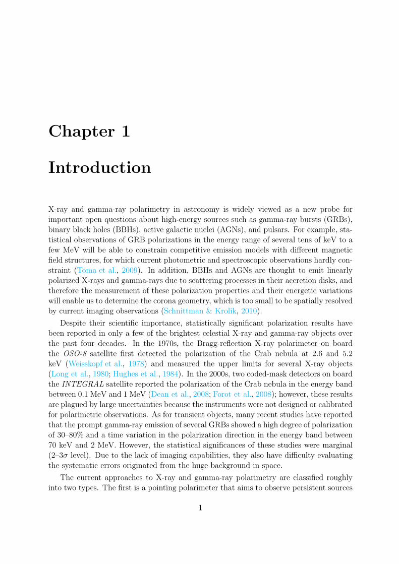
X-ray and gamma-ray polarimetry in astronomy is widely viewed as a new probe for
important open questions about high-energy sources such as gamma-ray bursts (GRBs),
binary black holes (BBHs), active galactic nuclei (AGNs), and pulsars. For example, sta-
tistical observations of GRB polarizations in the energy range of several tens of keV to a
few MeV will be able to constrain competitive emission models with different magnetic
field structures, for which current photometric and spectroscopic observations hardly con-
straint (Toma et al., 2009). In addition, BBHs and AGNs are thought to emit linearly
polarized X-rays and gamma-rays due to scattering processes in their accretion disks, and
therefore the measurement of these polarization properties and their energetic variations
will enable us to determine the corona geometry, which is too small to be spatially resolved
by current imaging observations (Schnittman & Krolik, 2010).
Despite their scientific importance, statistically significant polarization results have
been reported in only a few of the brightest celestial X-ray and gamma-ray objects over
the past four decades. In the 1970s, the Bragg-reflection X-ray polarimeter on board
the OSO-8 satellite first detected the polarization of the Crab nebula at 2.6 and 5.2
keV (Weisskopf et al., 1978) and measured the upper limits for several X-ray objects
(Long et al., 1980; Hughes et al., 1984). In the 2000s, two coded-mask detectors on board
the INTEGRAL satellite reported the polarization of the Crab nebula in the energy band
between 0.1 MeV and 1 MeV (Dean et al., 2008; Forot et al., 2008); however, these results
are plagued by large uncertainties because the instruments were not designed or calibrated
for polarimetric observations. As for transient objects, many recent studies have reported
that the prompt gamma-ray emission of several GRBs showed a high degree of polarization
of 30–80% and a time variation in the polarization direction in the energy band between
70 keV and 2 MeV. However, the statistical significances of these studies were marginal
(2–3σ level). Due to the lack of imaging capabilities, they also have difficulty evaluating
the systematic errors originated from the huge background in space.
The current approaches to X-ray and gamma-ray polarimetry are classified roughly
into two types. The first is a pointing polarimeter that aims to observe persistent sources
1
2
with a flux of 10–100 mCrab with high sensitivity (Soffitta et al., 2013; Beilicke et al.,
2014; Weisskopf et al., 2016; Iwakiri et al., 2016; Krawczynski et al., 2016; Chauvin et al.,
2016a; Katsuta et al., 2016). These polarimeters use a X-ray focusing mirror or a fine col-
limator to suppress the background which causes serious degradation in the polarization
sensitivity. The second approach is a wide field of view (FoV) polarimeter with large
detection area (Bloser et al., 2009; Yonetoku et al., 2011a; Orsi & Polar Collaboration,
2011; Gunji et al., 2014; Yatsu et al., 2014); these are dedicated to observations of bright
transient objects, especially prompt emissions of bright and short-duration GRBs. Even
though a wide FoV increases the chance of GRB detection, it also accepts a huge back-
ground contribution coming from all directions. Therefore, these polarimeters have dif-
ficulty observing low signal-to-noise ratio sources, such as persistent sources and long-
duration GRBs which last several tens of seconds or more. Even though these wide FoV
polarimeters require the uniform sensitivity in the whole FoV to suppress the systematic
effects, it is not yet realized. As mentioned above, there are no promising approaches to
simultaneously explore both persistent and transient polarized sources in the universe;
an X-ray or gamma-ray polarimeter with both a moderate sensitivity and a wide FoV is
required.
In the energy range from a few hundreds of keV to a few tens of MeV, Compton
cameras have been studied as gamma-ray imaging telescopes capable of polarimetry and
wide FoV. A clear gamma-ray image based on a well-defined point spread function (PSF)
could provide powerful background suppression by constraining the direction of incident
photons. However, the Imaging Compton telescope (COMTEPL) (Schoenfelder et al.,
1993), the only satellite-borne Compton camera, eventually indicated that it is difficult to
reduce the background sufficiently using gamma-ray images obtained by via conventional
Compton cameras (Weidenspointner et al., 2001; Schonfelder, 2004).
As a next-generation MeV gamma-ray telescope, we have demonstrated the per-
formance of an electron-tracking Compton camera (ETCC) utilizing a gaseous three-
dimensional electron tracker since 2004 (Tanimori et al., 2004). The fine electron tracking
enables us to reduce the PSF dramatically and consequently greatly improve the detection
and polarization sensitivity. In Tanimori et al. (2015), we experimentally demonstrated
that our ETCC has the ability to form a well-defined PSF of several degrees in the energy
range from 100 keV to a few MeV. Such a sharp PSF reduces a huge background contribu-
tion coming from all directions by nearly 3 orders of magnitude without any heavy shield,
similarly to the focusing telescope, compared to typical non-imaging gamma-ray detec-
tors such as coded-mask detectors and GRB polarimeters mentioned above. The satellite
model ETCC is expected to have an effective area of 240 cm2 with a PSF of 2 at 1 MeV,
and the detection sensitivity would reach 1 mCrab flux at 1 MeV in a 106 s observation
(Tanimori et al., 2015). Thanks to its powerful background suppression and wide FoV of
up to 2π sr (Matsuoka et al., 2015), an ETCC has the capabilities of a highly-sensitive
gamma-ray polarimeter that can be used not only to survey new faint persistent sources
but also to observe transient objects including GRBs.

3
In this thesis, we investigate the basic polarimetric performance of the ETCC using
both Monte Carlo simulations and experiments performed in the linearly polarized hard
X-ray beamline at SPring-8. We begin with an overview of the potential MeV gamma-ray
sources of polarized emission, including a theoretical predictions and the observational
polarization results. In Chapter 3, we explain the principles of a Compton polarimeter,
and how the polarization measurements are disturbed by the statistical and systematic
errors in space. In Chapter 4, we review the astronomical Compton polarimeters by divid-
ing them into the following four types: non-dedicated instruments, pointing polarimeters,
GRB polarimeters, and Compton cameras. In Chapter 5, we present the detector config-
urations and the performances of the ETCC. In Chapter 6, we describe the polarimetric
performance of the ETCC using the Monte Carlo simulation. In Chapter 7, we report
the analysis and results of the beam experiments. Finally, we discuss the polarization
sensitivities for future all-sky surveys using balloons and satellites in Chapter 8.

Chapter 2
Polarization in MeV Gamma-Ray
Astronomy
2.1 MeV Gamma-ray Sources
The gamma-ray imaging and spectroscopic survey in MeV region was only performed
by COMPTEL onbord Compton Gamma-Ray Observatory (CGRO) satellite launched in
1991 (Schoenfelder et al., 1993). As shown in Table 2.1, COMPTEL detected only 32
persistent sources and 31 transient sources in the 0.75–30 MeV band (Schonfelder et al.,
2000). The INTEGRAL/IBIS reported the catalogue of the all sky survey in the sub-
MeV band (100–300 keV), which includes 113 persistent sources at a significance above
5σ (Krivonos et al., 2015). These number of the detected sources in sub-MeV and MeV
bands are quite smaller than that of Swift and Fermi/LAT, which detected 1171 sources
in the 14–195 keV band (Baumgartner et al., 2013) and more than 3000 sources in the
0.1–100 GeV band (Nolan et al., 2012), respectively. This divergence is explained by the
poor sensitivity in MeV region as shown in Figure 2.1.
Despite of the large amount of imaging and spectroscopic observations in X-ray and
sub-GeV region, there are still remaining open questions, such as the prompt emission
mechanism of GRBs and the origin of the seed photons for inverse-Compton scattering
emission in AGNs. Therefore, we need not only to improve the imaging and spectroscopic
sensitivity in MeV band but also to use the polarization properties in addition to the
image and the energy spectrum of the astronomical objects.
2.2 Potential Sources of Polarized Emission
Polarization measurement provides two additional observational parameters, the degree
of polarization and the polarization direction of the source emission, which enables us to
discriminate the competing physics models. The only dedicated X-ray polarimetry mission
to date is the OSO-8 experiment, which detected the polarization of the Crab nebula at
4

2.2. POTENTIAL SOURCES OF POLARIZED EMISSION 5
Table 2.1: The detected sources with COMPTEL (Schonfelder et al., 2000).
Spin-Down Pulsars 3 Crab, Vela, PSR 1509-58Other Galactic sources 7 Cyg X-1, Crab Nebula, etc.Active Galactic Nuclei 10 Cen A, etc.Gamma-Ray Line Source 7 SN1991T (56Co), etc.Unidentified Sources 5Total Number 32Gamma-Ray Burst 31
Figure 2.1: Sensitivity for continuum in X-ray and gamma-ray region (Schonfelder, 2004).
2.6 and 5.2 keV (Weisskopf et al., 1978). The recent progress of X-ray detectors, such as
an increasing efficiency of the X-ray focusing mirrors, enables to design highly-sensitive
X-ray polarimeters (Soffitta et al., 2013; Weisskopf et al., 2016), whose sensitivities are
more than two orders of magnitude better than that of OSO-8. For those reasons, the
scientific importances of X-ray polarimetry (< 100 keV) has already been well discussed
(for recent review see Krawczynski et al. 2011, and Soffitta et al. 2013). In the following
section, we focus on the scientific importances of sub-MeV/MeV gamma-ray polarimetry
(> 100 keV) for GRBs, AGNs, BHBs, and Pulsars, according to the results of COMPTEL.
2.2.1 Gamma-Ray Bursts
Gamma-ray bursts (GRBs) are the most luminous transient objects in gamma-ray region,
whose luminosity reach 1054 erg s−1. Burst and Transient Source Experiment (BATSE)
on CGRO reveals that GRBs are isotropically distributed in the sky with an occurrence
rate of roughly one every day (Kouveliotou et al., 1993; Fishman, 1999). The observed
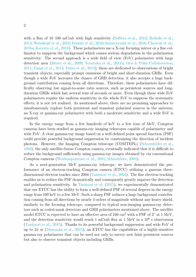
distribution of burst durations are shown in in Figure 2.2, which suggest that GRBs can be
separated into two classes, short events (< 2 s) and longer ones (> 2 s) (Kouveliotou et al.,
6 2.2. POTENTIAL SOURCES OF POLARIZED EMISSION
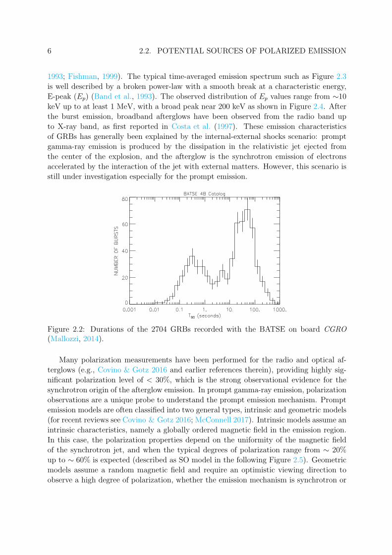
1993; Fishman, 1999). The typical time-averaged emission spectrum such as Figure 2.3
is well described by a broken power-law with a smooth break at a characteristic energy,
E-peak (Ep) (Band et al., 1993). The observed distribution of Ep values range from ∼10
keV up to at least 1 MeV, with a broad peak near 200 keV as shown in Figure 2.4. After
the burst emission, broadband afterglows have been observed from the radio band up
to X-ray band, as first reported in Costa et al. (1997). These emission characteristics
of GRBs has generally been explained by the internal-external shocks scenario: prompt
gamma-ray emission is produced by the dissipation in the relativistic jet ejected from
the center of the explosion, and the afterglow is the synchrotron emission of electrons
accelerated by the interaction of the jet with external matters. However, this scenario is
still under investigation especially for the prompt emission.
Figure 2.2: Durations of the 2704 GRBs recorded with the BATSE on board CGRO(Mallozzi, 2014).
Many polarization measurements have been performed for the radio and optical af-
terglows (e.g., Covino & Gotz 2016 and earlier references therein), providing highly sig-
nificant polarization level of < 30%, which is the strong observational evidence for the
synchrotron origin of the afterglow emission. In prompt gamma-ray emission, polarization
observations are a unique probe to understand the prompt emission mechanism. Prompt
emission models are often classified into two general types, intrinsic and geometric models
(for recent reviews see Covino & Gotz 2016; McConnell 2017). Intrinsic models assume an
intrinsic characteristics, namely a globally ordered magnetic field in the emission region.
In this case, the polarization properties depend on the uniformity of the magnetic field
of the synchrotron jet, and when the typical degrees of polarization range from ∼ 20%
up to ∼ 60% is expected (described as SO model in the following Figure 2.5). Geometric
models assume a random magnetic field and require an optimistic viewing direction to
observe a high degree of polarization, whether the emission mechanism is synchrotron or
2.2. POTENTIAL SOURCES OF POLARIZED EMISSION 7
Figure 2.3: Energy spectrum of GRB 990123(Briggs et al., 1999).
Figure 2.4: Distributions of Ep
(Goldstein et al., 2013).
inverse Compton. The typical degree of polarization is < 20% for most viewing angles,
although synchrotron emission can produce the degree of polarization as high as ∼ 70%
(SR model), and inverse Compton models (CD model) can achieve ∼ 100% of degree of
polarization under optimistic geometries. Therefore, the intrinsic and geometric models
can be distinguished by a statistical study of polarization properties in prompt emission
(Toma et al., 2009). In particular, the dependence of the degree of polarization on Ep can
be a clear diagnostic, as shown in Figure 2.5.
The polarimetric observations of the prompt gamma-ray emission to date are summa-
rized in Table 2.2. These studies have reported a high degree of polarization of 30%–80%
and a time variation in the polarization signatures in some GRBs. Some authors sug-
gested that the prompt emissions of the GRBs are more likely to originate in synchrotron
radiation, and the direction of the magnetic field varies temporally or spatially. How-
ever the statistical significances of all studies were marginal, typically having a confidence
level of 2–3σ. Even in the experiments by the Gamma-Ray Burst Polarimeter (GAP;
Yonetoku et al. 2011a), which is optimized for the GRB polarimetry, only three GRBs
are detected with the significance of 3σ level (<3.7σ).

8 2.2. POTENTIAL SOURCES OF POLARIZED EMISSION
Figure 2.5: Simulated distribution of the degree of polarization as a function of Ep inthe SO (red open circles), SR (green filled circles), and CD (blue plus signs) models(Toma et al., 2009).

2.2. POTENTIAL SOURCES OF POLARIZED EMISSION 9
Table 2.2: GRB polarization observations for prompt gamma-ray emission. Table adaptedfrom McConnell (2017).
Pub Energy Degree ofDate GRB Instrument (keV) Polarization
2004 GRB 021206 RHESSI 150–2000 80%±20%2004 GRB 021206 RHESSI 150–2000 < 4.1%2004 GRB 021206 RHESSI 150–2000 41+57
−44%2005 GRB 930131 CGRO/BATSE 20–1000 (35–100%)a
2005 GRB 960924 CGRO/BATSE 20–1000 (50–100%)a
2007 GRB 041219a INTEGRAL/SPI 100–350 98%±33%2007 GRB 041219a INTEGRAL/SPI 100–350 96%±40%2009 GRB 041219a INTEGRAL/IBIS 200–800 43%±25%b
2009 GRB 061122 INTEGRAL/SPI 100–1000 < 60%2011 GRB 100826a IKAROS/GAP 70–300 27%±11%c
2012 GRB 110301a IKAROS/GAP 70–300 70%±22%2012 GRB 110721a IKAROS/GAP 70–300 80%±22%2013 GRB 061122 INTEGRAL/IBIS 250–800 > 60%2014 GRB 140206a INTEGRAL/IBIS 200–800 > 48%2016 GRB 151006a Astrosat/CZTI 100–300 –
a albedo polarimetryb variable degree of polarizationc variable polarization angle

10 2.2. POTENTIAL SOURCES OF POLARIZED EMISSION
Figure 2.6: The schematic view of AGN.Retrieved from https://heasarc.gsfc.nasa.gov/docs/cgro/images/epo/gallery/agns/index.html
2.2.2 Active Galactic Nuclei
An active galactic nucleus (AGN) is thought to be a compact region at the center of a
host galaxy with a strong broadband emission. The radiation from an AGN is believed
to be a result of accretion of matter by a supermassive black hole at the center of its host
galaxy. Figure 2.6 shows the schematic view of the unified model of AGN. Radio and
optical band observation indicates that many AGN have relativistic jet outflows. The
AGNs dominated by relativistic jets pointing in our direction are commonly known as
blazars. Blazars are characterized by a non-thermal spectral energy distribution, where
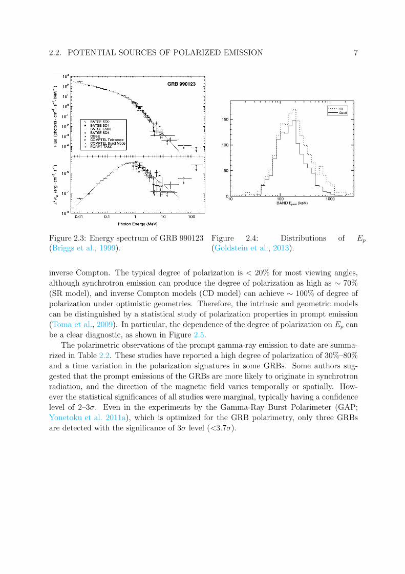
two broad components exhibit as shown in Figure 2.7. The low-energy component is in
the range of radio to UV or even X-rays, and the high-energy component starts from the
X-ray band and can reach TeV or even higher energies. The high-energy component of
flat-spectrum radio quasar (FSRQ) type blazars is expected to be peaked in MeV band
as shown on the left in Figure 2.7.
It is expected that the low-energy component is due to the synchrotron radiation of
the relativistic electrons. Indeed, measurements in the radio and optical bands showed a
polarization level of a few percent up to as much as 40%. The high-energy component
is construed to be typically associated with inverse-Compton scattering of low-energy
photons (leptonic models), although the origin of the seed photons is less well understood.
The polarization measurement would be the key to distinguish between the following
scenarios: (i) Seed photons are the synchrotron photons emitting in the optical/UV band
(synchrotron self Compton model). In this case, the polarization of the hard X-rays is
expected to track the polarization at radio and optical bands. If the magnetic fields are
perfectly ordered, the degree of polarization would reach > 30% (Poutanen, 1994). (ii)
2.2. POTENTIAL SOURCES OF POLARIZED EMISSION 11
Seed photons are the accretion disk photons or the emission coming from broad line region
(external Compton model). In this case, the high-energy component will have a relatively
small fraction of polarization (<10%) (McNamara et al., 2009).
It has been pointed out that high energy proton in the jet can be induced by hadronic
interactions (hadronic model). Because of the dominance of synchrotron radiation in
hadronic models, a high polarization is expected compared to that for leptonic models
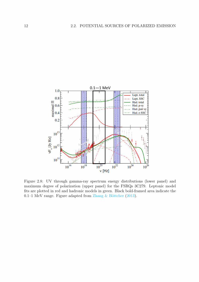
(Zhang & Bottcher, 2013). In the case of famous FSRQ-type blazar 3C279, as shown in
Figure 2.8, the degree of polarization of hadronic models is over 0.6 in the wide energy
band, on the other hand that of leptonic models approaches to 0 as increased the energy.
Figure 2.7: The broadband spectral energy distribution of the FSRQ-type blazar3C279 (left panel) and the high-synchrotron-peak BL-type blazar Mkn421 (right panel)(Madejski & Sikora, 2016).
12 2.2. POTENTIAL SOURCES OF POLARIZED EMISSION
Figure 2.8: UV through gamma-ray spectrum energy distributions (lower panel) andmaximum degree of polarization (upper panel) for the FSRQs 3C279. Leptonic modelfits are plotted in red and hadronic models in green. Black bold-framed area indicate the0.1–1 MeV range. Figure adapted from Zhang & Bottcher (2013).

2.2. POTENTIAL SOURCES OF POLARIZED EMISSION 13
Figure 2.9: The energy spectra of Cygnus X-1 in soft state, hard state, and intermediatestate (Zdziarski et al., 2002).
2.2.3 Binary Black Holes
In the final evolution of a massive star with a mass above 30M⊙, the core is considered
to collapse to a black hole after a type II supernova. Binary black hole (BHB) is a binary
system with a black hole and a companion star, where an accretion disk is created because
the matter from the companion star flows onto the black hole. This accretion disk radiates
photons in wide band including X-rays and gamma-rays.
It is well known that BHB transit through different spectral states during their out-
bursts. The two main states are the soft state and the hard state. In addition, the
intermediate state exists between the soft and hard state. Figure 2.9 shows the spectra
of the soft, hard and intermediate state of Cyg X-1, which is one of the most well-studied
black hole binary. The X-ray spectrum in the soft state is generally associated with a
blackbody radiation from the accretion disk with a characteristic temperature of ∼ 1
keV. In the hard state, the X-ray and γ-ray spectrum is generally described by a power
law model with an exponential cutoff at about 100 keV. The standard explanation for
the high energy emission is a inverse Compton scattering of disk photons by hot (∼ 100
keV) thermal electrons (corona) in the inner region of the accretion flow and its reflection
component at the disk. However, it has been observed that some bright sources exhibit an
excess of emission above 300 keV, extending to the MeV range, whose emission mechanism
is still under debate.
X-ray and gamma-ray polarization measurement of BHB is conventionally expected as
the probe to investigate the geometrical distribution of corona in hard state.Schnittman & Krolik
(2010) calculated the expected polarization signatures for various corona geometries be-

14 2.2. POTENTIAL SOURCES OF POLARIZED EMISSION
low 100 keV, and they predicted that the degree of polarization would be < 10% for any
corona geometries even with small differences. Recent findings of high polarization in
Cygnus X-1 by INTEGRAL suggests that gamma-ray polarization measurements enable
us to understand the emission mechanism of the high-energy tail. Laurent et al. (2011)
reported that the degree of polarization of Cygnus X-1 between 400 keV and 2 MeV is
67±30%, whereas they obtained only a 20% upper limit in the 250–400 keV band. Its
high degree of polarization suggests that the high-energy tail is due to synchrotron emis-
sion from a compact jet. An alternative model was introduced by Romero et al. (2014),
where the MeV tail is the synchrotron radiation of secondary non-thermal electrons in
the corona. This coronal model also predicts significant polarization during intermedi-
ate states, therefore this can be tested in the future sub-MeV gamma-ray polarimetric
observations (Romero et al., 2014).
2.2.4 Pulsars
Pulsars radiate a short periodic pulse, and hence are considered to be neutron stars
spinning with a high speed. A neutron star also has a strong magnetic field of about 1012
G. Because the magnetic axis inclines to the rotation axis generally, the emission near the
magnetic poles sweeps around the rotation axis. Since the emission region of the pulsar
rotating around the axis is observed from the earth, we see it like a light house. Within
thousand pulsars observed so far, the emission of MeV gamma-rays are only observed
from several of them.
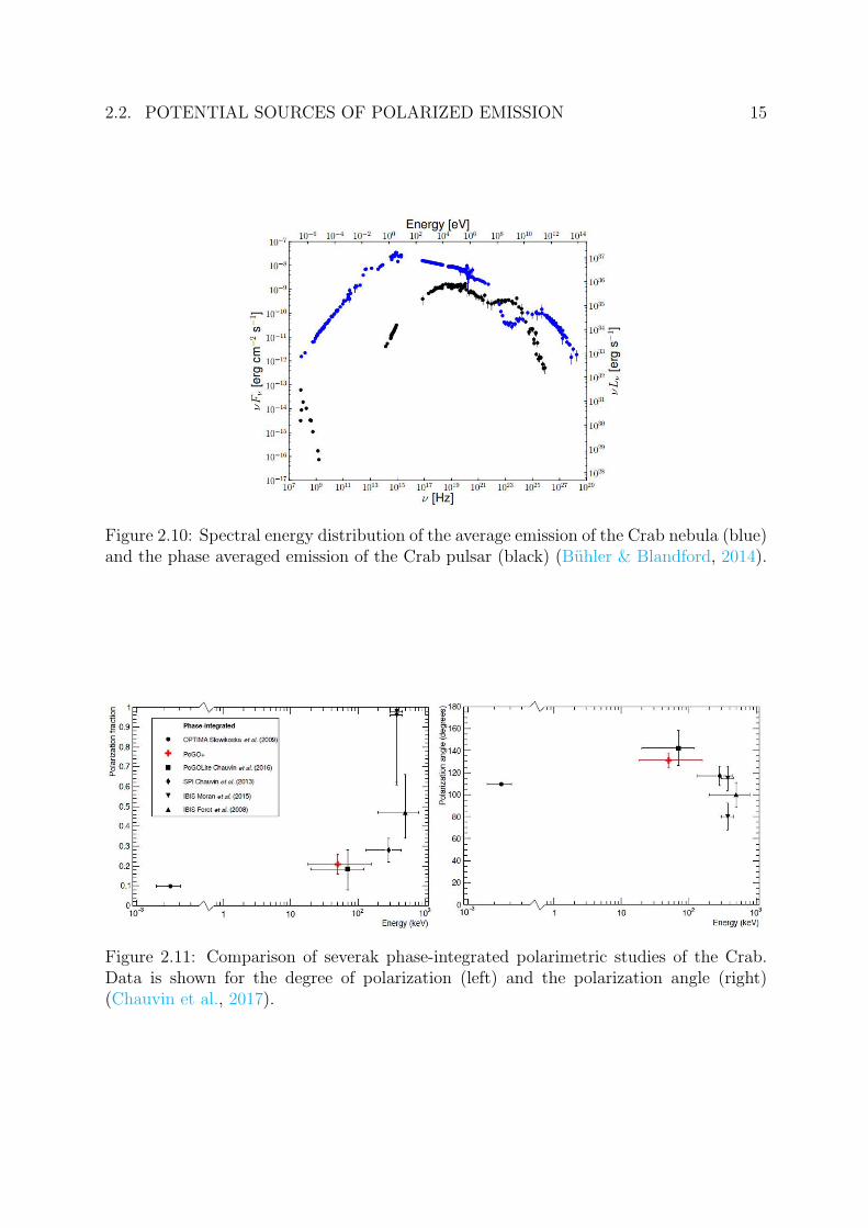
The Crab pulsar, one of the most famous pulsars, has a nebula around it. The Crab
pulsar and the Crab nebula have been well observed from the radio to the TeV gamma-
ray as shown in Figure 2.10. In the MeV range, both the pulsar and nebular components
contribute significantly to the total emission. The hard X-ray and gamma-ray emission is
explained by synchrotron radiation and at higher energies via inverse Compton scattering.
The bright synchrotron radiation is a good probe for detailed studies of the inner region
of the Crab pulsar and the Crab nebula. The polarized gamma-ray emission from the
nebula and pulsar have been measured, having a confidence level of 5σ. The results
of these measurements are summarized in Figure 2.11. More precise measurements are
required to confirm the energy dependence or the time variation of the polarization states.
2.2. POTENTIAL SOURCES OF POLARIZED EMISSION 15
Figure 2.10: Spectral energy distribution of the average emission of the Crab nebula (blue)and the phase averaged emission of the Crab pulsar (black) (Buhler & Blandford, 2014).
Figure 2.11: Comparison of severak phase-integrated polarimetric studies of the Crab.Data is shown for the degree of polarization (left) and the polarization angle (right)(Chauvin et al., 2017).

Chapter 3
Compton Gamma-ray Polarimetry
3.1 Polarization Modulation
3.1.1 Compton Scattering Cross Section
The polarization states of photons are quantified by the degree of polarization and the
polarization angle. In the energy range from approximately 50 keV to several MeV, where
the dominant interaction is the Compton scattering, they are determined by measuring
the statistical distribution of Compton scattering angle, which is modulated according to
the polarization states.
In this section, we derive the intensity of Compton scattered photons when the light
source is partially polarized. To evaluate the modulation of the intensity properly, we
require careful attention to the coordinate systems for measurement. Figure 3.1 shows
a schematic view of Compton scattering of a polarized photon, where the photon polar
coordinate system is denoted as (θph, ϕph). The differential cross section of Compton
scattering by a free electron is given by the Klein-Nishina formula (Klein & Nishina,
1929). For unpolarized photons this is given by,
fUnP(θph) =r202
E2
E02
(E0
E+
E
E0
− sin2 θph
), (3.1)
where r0 is the classical electron radius, E0 and E are the incident and scattered photon
energies, respectively. E is given by,
E =E0
1 + E0
mec2(1− cos θph)
. (3.2)
In the case of completely polarized photons, the differential cross section is expressed as
(e.g., Lei et al. (1997) and references therein),
fPol(θph, ηph) =r202
E2
E02
(E0
E+
E
E0
− 2 sin2 θph cos2 ηph
), (3.3)
16
3.1. POLARIZATION MODULATION 17
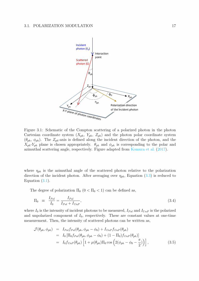
Figure 3.1: Schematic of the Compton scattering of a polarized photon in the photonCartesian coordinate system (Xph, Yph, Zph) and the photon polar coordinate system(θph, ϕph). The Zph-axis is defined along the incident direction of the photon, and theXph-Yph plane is chosen appropriately. θph and ϕph is corresponding to the polar andazimuthal scattering angle, respectively. Figure adapted from Komura et al. (2017).
where ηph is the azimuthal angle of the scattered photon relative to the polarization
direction of the incident photon. After averaging over ηph, Equation (3.3) is reduced to
Equation (3.1).
The degree of polarization Π0 (0 < Π0 < 1) can be defined as,
Π0 ≡ IPolI0
=IPol
IPol + IUnP
, (3.4)
where I0 is the intensity of incident photons to be measured, IPol and IUnP is the polarized
and unpolarized component of I0, respectively. These are constant values at one-time
measurement. Then, the intensity of scattered photons can be written as,
J (θph, ϕph) = IPolfPol(θph, ϕph − ϕ0) + IUnPfUnP(θph)
= I0 [Π0fPol(θph, ϕph − ϕ0) + (1− Π0)fUnP(θph)]
= I0fUnP(θph)[1 + µ(θph)Π0 cos
(2(ϕph − ϕ0 −
π
2))]
, (3.5)

18 3.1. POLARIZATION MODULATION
where ϕ0 is the polarization angle of incident photon, and µ(θph) is given by,
µ(θph) =sin2 θph
E0/E + E/E0 − sin2 θph. (3.6)
Plots of µ(θph) for various E0 are shown in Figure 3.2.
Figure 3.2: Dependences of µ on θph for various E0. Figure adapted from Lei et al. (1997).
3.1.2 On-axis measurement
J (θph , ϕph) includes Π0 and ϕ0 in a simple form, in which Π0 and ϕ0 correspond to
the amplitude and the phase angle of cos (2ϕph)-curve, respectively. Therefore Π0 and
ϕ0 are determined by measuring J (θph , ϕph), which is the basic principle of Compton
polarimetry. However, quantities measured by polarimeters are recorded in the detector
coordinate system, which is generally different from the photon coordinate system. The
three dimensional angular distribution of scattered photons measured in the detector
coordinate system is expressed as,
D(θdet, ϕdet) = J (θdet, ϕdet)ϵ(θdet, ϕdet), (3.7)
where θdet and ϕdet are the polar and azimuthal angle in the detector coordinates, respec-
tively, J (θdet, ϕdet) is J (θph, ϕph) that is transformed from the photon coordinates, and
ϵ(θdet, ϕdet) is the detection efficiency of the detector. Also, the two dimensional angular
distribution is given by,
N (ϕdet) =
∫ θmax
θmin
D(θdet, ϕdet) sin θdetdθdet. (3.8)
3.1. POLARIZATION MODULATION 19
In addition, the number of photons (constant value) can be calculated as,
N0 =
∫ 2π
0
N (ϕdet)dϕdet. (3.9)
In the simplest case when the detector coordinates coincide with the photon coordi-
nates (in the case of on-axis incidence), N (ϕdet) is explicitly described as,
N (ϕdet) =I0
∫ θmax
θmin
fUnP(θdet)
×[1 + µ(θdet)Π0 cos
(2(ϕdet − ϕ0 −
π
2))]
ϵ(θdet, ϕdet) sin θdetdθdet.
(3.10)
If we assume ϵ(θdet, ϕdet) is equal to 1, N (ϕdet) follows a cos(2ϕdet) function as described
by
N (ϕdet) =N0
2π
[1 + µΠ0 cos
(2(ϕdet − ϕ0 −
π
2))]
, (3.11)
where,
µ =
∫ θmax
θminfUnP(θdet)µ(θdet) sin θdetdθdet∫ θmax
θminfUnP(θdet) sin θdetdθdet
, (3.12)
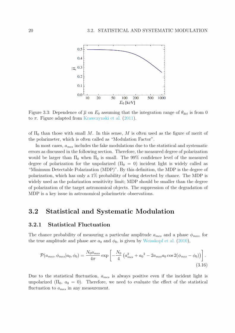
which is plotted in Figure 3.3 as a function of E0. In this case, the polarization modulation
follows a cos(2ϕdet)-curve with the amplitude of µΠ0 and the phase angle of ϕ0. We can
uniquely determine the Π0 and ϕ0 by fitting N (ϕdet) with the function such as,
g(ϕ) = C[1 + ames cos
(2(ϕ− ϕmes −
π
2))]
, (3.13)
where C is the constant of proportionality, and ames and ϕmes are the amplitude (0 <
ames < 1) and the phase angle (0 < ϕmes < 2π) to be measured, respectively. By compar-
ing Equation (3.11) with Equation (3.13), ames is assumed to be directly proportional to
Π0. Here we define the factor of proportionality as
M ≡ ames
Π0
(0 < M < 1). (3.14)
When N (ϕdet) is measured with very high precision and there is no statistical and sys-
tematic errors described in the following sections, M is equal to µ; otherwise M have to
be determined by the simulations and measurements. If M is known, Π0 is calculated by
Π0 =ames
M. (3.15)
According to Equation (3.15), polarimeters with large M is more sensitive to the change
20 3.2. STATISTICAL AND SYSTEMATIC MODULATION
Figure 3.3: Dependence of µ on E0 assuming that the integration range of θdet is from 0to π. Figure adapted from Krawczynski et al. (2011).
of Π0 than those with small M . In this sense, M is often used as the figure of merit of
the polarimeter, which is often called as “Modulation Factor”.
In most cases, ames includes the fake modulations due to the statistical and systematic
errors as discussed in the following section. Therefore, the measured degree of polarization
would be larger than Π0 when Π0 is small. The 99% confidence level of the measured
degree of polarization for the unpolarized (Π0 = 0) incident light is widely called as
“Minimum Detectable Polarization (MDP)”. By this definition, the MDP is the degree of
polarization, which has only a 1% probability of being detected by chance. The MDP is
widely used as the polarization sensitivity limit; MDP should be smaller than the degree
of polarization of the target astronomical objects. The suppression of the degradation of
MDP is a key issue in astronomical polarimetric observations.
3.2 Statistical and Systematic Modulation
3.2.1 Statistical Fluctuation
The chance probability of measuring a particular amplitude ames and a phase ϕmes , for
the true amplitude and phase are a0 and ϕ0, is given by Weisskopf et al. (2010),
P(ames , ϕmes|a0, ϕ0) =N0ames
4πexp
[−N0
4
(a2mes + a0
2 − 2amesa0 cos 2(ϕmes − ϕ0))]
.
(3.16)
Due to the statistical fluctuation, ames is always positive even if the incident light is
unpolarized (Π0, a0 = 0). Therefore, we need to evaluate the effect of the statistical
fluctuation to ames in any measurement.

3.2. STATISTICAL AND SYSTEMATIC MODULATION 21
Figure 3.4: Probability distribution of ames due to the statistical fluctuation, for an un-polarized source (a0 = 0) assuming N0 = 104. The region of integration in Equation 3.18is shown by the hatched area.
For unpolarized case, Equation (3.16) is integrated over ϕmes analytically. The prob-
ability distribution of ames is therefore,
P(ames) =N0ames
2exp
(−N0
4a2mes
), (3.17)
which is plotted in Figure 3.4 assuming N0 = 104. Now the 99% confidence interval a99%is calculated from the following equation:
N0
2
∫ a99%
0
ames exp
(−N0
4a2mes
)dames = 0.99. (3.18)
Then we get a99% as,
a99% =4.29√N0
. (3.19)
According to the definition provided in the previous section, MDP at 99% confidence
level is calculated as the degree of polarization corresponding to a99%:
MDP =4.29
M√N0
. (3.20)
N0 is determined by the multiplication of the source flux, the effective area of the po-
larimeter, and the exposure time. Therefore, a polarimeter has to be designed to have a
large effective area and large M to improve the MDP.
22 3.2. STATISTICAL AND SYSTEMATIC MODULATION
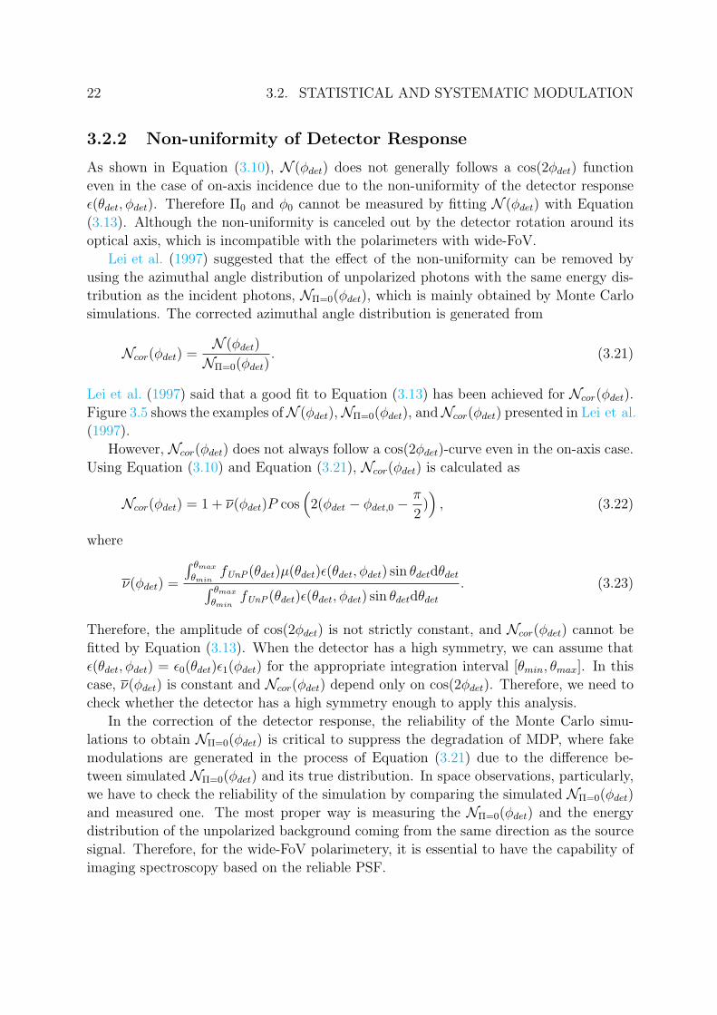
3.2.2 Non-uniformity of Detector Response
As shown in Equation (3.10), N (ϕdet) does not generally follows a cos(2ϕdet) function
even in the case of on-axis incidence due to the non-uniformity of the detector response
ϵ(θdet, ϕdet). Therefore Π0 and ϕ0 cannot be measured by fitting N (ϕdet) with Equation
(3.13). Although the non-uniformity is canceled out by the detector rotation around its
optical axis, which is incompatible with the polarimeters with wide-FoV.
Lei et al. (1997) suggested that the effect of the non-uniformity can be removed by
using the azimuthal angle distribution of unpolarized photons with the same energy dis-
tribution as the incident photons, NΠ=0(ϕdet), which is mainly obtained by Monte Carlo
simulations. The corrected azimuthal angle distribution is generated from
Ncor(ϕdet) =N (ϕdet)
NΠ=0(ϕdet). (3.21)
Lei et al. (1997) said that a good fit to Equation (3.13) has been achieved for Ncor(ϕdet).
Figure 3.5 shows the examples ofN (ϕdet),NΠ=0(ϕdet), andNcor(ϕdet) presented in Lei et al.
(1997).
However, Ncor(ϕdet) does not always follow a cos(2ϕdet)-curve even in the on-axis case.
Using Equation (3.10) and Equation (3.21), Ncor(ϕdet) is calculated as
Ncor(ϕdet) = 1 + ν(ϕdet)P cos(2(ϕdet − ϕdet,0 −
π
2)), (3.22)
where
ν(ϕdet) =
∫ θmax
θminfUnP(θdet)µ(θdet)ϵ(θdet, ϕdet) sin θdetdθdet∫ θmax
θminfUnP(θdet)ϵ(θdet, ϕdet) sin θdetdθdet
. (3.23)
Therefore, the amplitude of cos(2ϕdet) is not strictly constant, and Ncor(ϕdet) cannot be
fitted by Equation (3.13). When the detector has a high symmetry, we can assume that
ϵ(θdet, ϕdet) = ϵ0(θdet)ϵ1(ϕdet) for the appropriate integration interval [θmin, θmax]. In this
case, ν(ϕdet) is constant and Ncor(ϕdet) depend only on cos(2ϕdet). Therefore, we need to
check whether the detector has a high symmetry enough to apply this analysis.
In the correction of the detector response, the reliability of the Monte Carlo simu-
lations to obtain NΠ=0(ϕdet) is critical to suppress the degradation of MDP, where fake
modulations are generated in the process of Equation (3.21) due to the difference be-
tween simulated NΠ=0(ϕdet) and its true distribution. In space observations, particularly,
we have to check the reliability of the simulation by comparing the simulated NΠ=0(ϕdet)
and measured one. The most proper way is measuring the NΠ=0(ϕdet) and the energy
distribution of the unpolarized background coming from the same direction as the source
signal. Therefore, for the wide-FoV polarimetery, it is essential to have the capability of
imaging spectroscopy based on the reliable PSF.

3.2. STATISTICAL AND SYSTEMATIC MODULATION 23
Figure 3.5: Azimuthal angle distributions of scattered photons calculated by the MonteCarlo simulation of COMPTEL; top left) unpolarized incident photons, NΠ=0(ϕdet); topright) completely polarized photons, N (ϕdet); bottom) corrected distribution, Ncor(ϕdet)and its best fit with cos(2ϕdet) function. The incident photons are on-axis with energy of1 MeV (Lei et al., 1997).

24 3.2. STATISTICAL AND SYSTEMATIC MODULATION
3.2.3 Off-axis Incidence
Figure 3.6: Schematic of Compton scattering in the case of off-axis incidence in thedetector Cartesian coordinate system (Xdet , Ydet , Zdet) and polar coordinate system (θdet ,ϕdet). The Zdet-axis is defined along the optical axis of the detector, and the Xdet-Ydet
plane is chosen appropriately. The travel direction of incident photon is described as (α,β). The remaining symbols have the same meaning as in Figure 3.1. Figure adapted fromKomura et al. (2017).
As shown in Figure 3.6, when the incident photon has an incident angle of α rela-
tive to the optical axis of the detector (in the case of off-axis incidence), the detector
coordinates are not coincident with the photon coordinates. Therefore, N (ϕdet) described
in Equation (3.8) have to be transformed to this coordinates using Equation (3.7), and
then transformed N (ϕdet) follows a cos(2ϕdet) function. Then, nontransformed N (ϕdet)
possibly cause fake modulations even for unpolarized photons (Lei et al., 1997; Muleri,
2014).
If the polarimeter measures θdet in addition to ϕdet event by event, we can move
to the photon coordinate system photon by photon, where cos (2ϕ)-curve is recovered
(Lei et al., 1997). The displacement of the scattered photon in the photon coordinate
system from the detector coordinate system is calculated by the following transformation

3.2. STATISTICAL AND SYSTEMATIC MODULATION 25
matrix (Lei et al., 1997; Muleri, 2014):xph = (xdet cos β + ydet sin β) cosα− zdet sinα,
yph = −xdet sin β + ydet cos β,
zph = (xdet cos β + ydet sin β) sinα− zdet cosα,
(3.24)
where (xdet , ydet , zdet) is the displacement of the scattered photon in the detector coordi-
nate system and (α, β) are the polar and azimuthal angle of incident photon, respectively.
Now, we calculate the angular distribution of the scattered photon D(θph, ϕph). Then,
the integrated azimuthal angle distribution N (ϕph) is expressed as,
N (ϕdet) =
∫ θmax
θmin
D(θph, ϕph) sin θphdθph
= I0
∫ θmax
θmin
fUnP(θph)
×[1 + µ(θph)P cos
(2(ϕph − ϕph,0 −
π
2))]
ϵ(θph, ϕph) sin θphdθph.
(3.25)
Although N (ϕph) includes ϵ(θph, ϕph), the same analysis in Section 3.2.2 removes the non-
uniformity and recovers the cos(2ϕph)-curve. Figure 3.7 shows the example. Lei et al.
(1997) said that a polarization modulation is visible only after the removal of the modu-
lations due to the off-axis incidence and the non-uniformity of the detector response and
can be fitted by Equation (3.13).
Unfortunately, the most of Compton polarimeters do not measure θdet . Therefore,
it is difficult to perform the coordinate transformation and to cancel out the effect of
off-axis incidence and detector response even if reliable NΠ=0(ϕdet) is obtained in some
way. Several authors have reported that M of their developed GRB polarimeters, which
is discussed in Chapter 4, decreased by approximately 40% for an incident angle of 60 in
Monte Carlo simulations (Xiong et al., 2009; McConnell et al., 2009; Gunji et al., 2014)
due to the lack of θdet . Figure 3.8 shows the dependence of the simulated M on incident
angles for a certain model of POLAR detector. Due to the degradation of M , MDP is
increased by more than 1.7 times according to Equation (3.20) when the incident angle is
larger than 60, where the solid angle corresponds to the half of the 2Π-steradian-FoV. As
a result, the measurement of θdet is essential for the wide-FoV polarimetry in principle.

26 3.2. STATISTICAL AND SYSTEMATIC MODULATION
Figure 3.7: An example of the removal of off-axis incidence effect from a polarized datasetto reveal the underlying polarimetric distribution. The detector configuration used in thesimulation is the COMPTEL. Incident photons are 15 off-axis. : top left) unpolarizedincident photons, NΠ=0(ϕph); top right) completely polarized photons, N (ϕph); bottom)
corrected distribution, Ncor(ϕph) and its best fit with cos(2ϕdet) function (Lei et al., 1997).

3.2. STATISTICAL AND SYSTEMATIC MODULATION 27
Figure 3.8: The simulated modulation factors of a certain model of POLAR detector.They varies with incident angle theta but remains almost constant with polarizationangle phi (Xiong et al., 2009).
28 3.3. BACKGROUND NOISE IN SPACE
3.3 Background Noise in Space
In astronomical observations of hard X-ray and MeV gamma-ray, the background noise
is always the dominant signal. Cosmic rays interact with the instruments and satellites
and produce large amount of gamma rays by the nuclear reaction and Bremsstrahlung.
Thus, MeV gamma-rays generated in the satellite are dominant background source. The
shielding of MeV gamma-rays is also difficult due to their high transmittance. The large
fake modulations in N (ϕdet) are usually produced by these various types of background
with anisotropic directional distributions.
In order to minimize the background effect, its distribution has to be measured by an
on-source/off-source observation strategy or derived by detailed modeling although sim-
ulated background distribution contains large uncertainty in most cases. Any residual of
background in N (ϕdet) would lead to the degradation of M and introduce fake modula-
tions after the correction and transformation of Equations (3.21) and (3.24). These fake
modulations reduce the MDP systematically.
Even if background is well understood and properly removed, it reduces the MDP
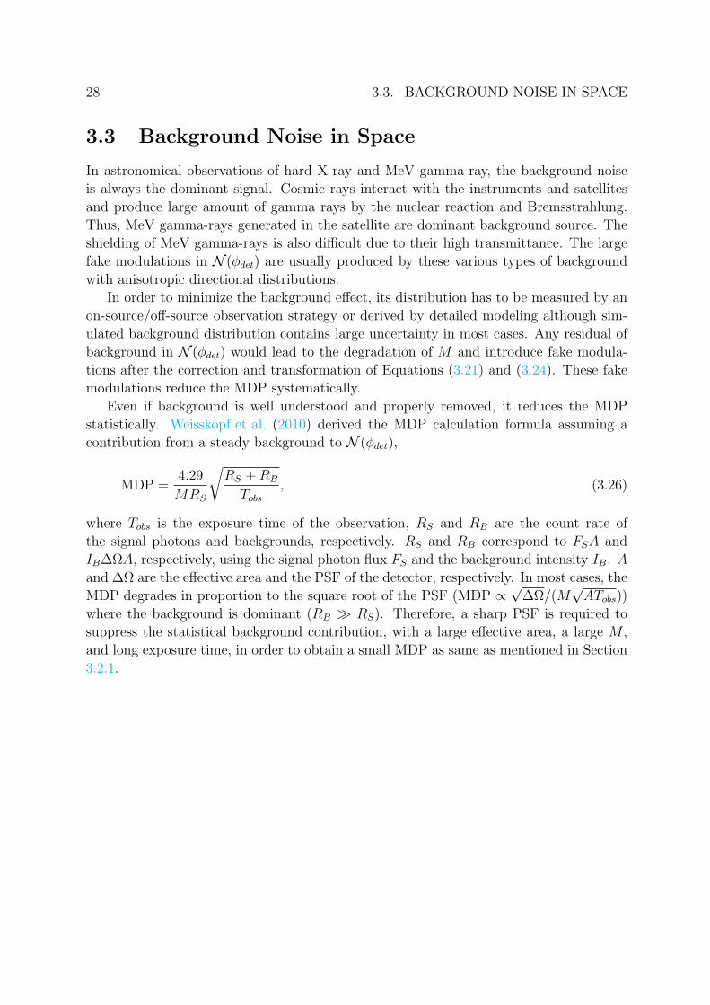
statistically. Weisskopf et al. (2010) derived the MDP calculation formula assuming a
contribution from a steady background to N (ϕdet),
MDP =4.29
MRS
√RS +RB
Tobs
, (3.26)
where Tobs is the exposure time of the observation, RS and RB are the count rate of
the signal photons and backgrounds, respectively. RS and RB correspond to FSA and
IB∆ΩA, respectively, using the signal photon flux FS and the background intensity IB. A
and ∆Ω are the effective area and the PSF of the detector, respectively. In most cases, the
MDP degrades in proportion to the square root of the PSF (MDP ∝√∆Ω/(M
√ATobs))
where the background is dominant (RB ≫ RS). Therefore, a sharp PSF is required to
suppress the statistical background contribution, with a large effective area, a large M ,
and long exposure time, in order to obtain a small MDP as same as mentioned in Section
3.2.1.

Chapter 4
Astronomical Compton Polarimeters
As discussed in Chapter 3, the polarization of emission source is simply obtained by the
measurement of N (ϕdet). There were several challenges to measure N (ϕdet) of celestial ob-
jects by using sub-MeV and MeV gamma-ray instruments, such as CGRO/COMPTEL,
RHESSI, INTEGRAL/SPI and IBIS, and AstroSat/CZTI. However, high quality mea-
surements of the polarization were difficult due to their low modulation factor and a large
uncertainty of the systematic modulations. Recently, several types of dedicated Compton
polarimeters have been proposed depending on their target celestial objects. In this sec-
tion, I briefly summarize these astronomical gamma-ray instruments where the principle
of Compton polarimetry is utilized.
4.1 Non-dedicated Instruments
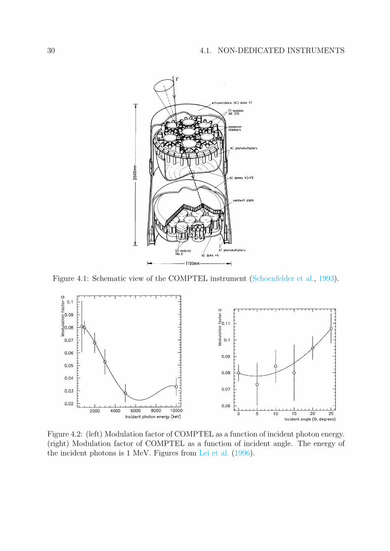
COMPTEL
COMPTEL is a unique Compton cameras used in space, which consists of forward liquid-
organic and backward NaI(Tl) scintillators as shown in Figure 4.1. The energy range
of COMPTEL is 0.8–30 MeV, and the effective is 20–50 cm2, which is reduced to the
half after the event selections are applied to the data. A Compton camera measures the
momentum of scattered photon in Compton scattering processes, and reconstructs the
direction as like the event circle. Therefore, COMPTEL were able to measure the three-
dimensional direction of the scattered gamma-ray and the polarization states of incident
photon. The simulation study of COMPTEL (Lei et al., 1996) shows that COMPTEL
has very small modulation factor ∼0.01 as shown in Figure 4.2, due to the geometrical
configuration where the forward scattering events were dominant. You note that these
modulation factors are obtained using the analysis of the cancellation of the systematic
modulations shown in Equation (3.21) and (3.24). In addition to the small modulation
factor, the huge background in space was not sufficiently removed by the Compton camera
imaging (Weidenspointner et al., 2001; Schonfelder, 2004). Consequently, COMPTEL did
not measure any statistically significant polarizations.
29
30 4.1. NON-DEDICATED INSTRUMENTS
Figure 4.1: Schematic view of the COMPTEL instrument (Schoenfelder et al., 1993).
Figure 4.2: (left) Modulation factor of COMPTEL as a function of incident photon energy.(right) Modulation factor of COMPTEL as a function of incident angle. The energy ofthe incident photons is 1 MeV. Figures from Lei et al. (1996).

4.1. NON-DEDICATED INSTRUMENTS 31
RHESSI
The Reuven Ramaty High Energy Solar Spectroscopic Imager (RHESSI) is a solar gamma-
ray telescope designed to make imaging and spectroscopic observations of solar flares at
energies between 3 keV and 20 MeV (Smith et al., 2002) using a coded mask. RHESSI
has an array of nine coaxial Germanium (Ge) detectors, as shown in Figure 4.3, which are
unshielded, and therefore GRBs are frequently observed. Although there is no positional
information available inside a Ge detector, these Ge detectors can be used as a Compton
polarimeter in the 0.15–2 MeV range since Nmes(ϕdet) is constructed from the coincidence
events that scatter between detectors (McConnell et al., 2002). RHESSI rotates at a
rate of ∼ 15 rotations per minute, which help to reduce the geometrical non-uniformity
response when the GRB placed near on-site. Coburn & Boggs (2003) obtained Nmes(ϕdet)
for extremely bright GRB (GRB 021206) using the RHESSI data (see Figure 4.4) and
reported the high degree of polarization of 80 ± 20% with a significance of 5.7σ, even
though subsequent studies of the data done by other authors did not confirm the initial
result (Wigger et al., 2004; Rutledge & Fox, 2004). Thus, these results are still conflict.
Figure 4.3: The RHESSI spectrometer array consists of nine Germanium detectors. EachGe detector is 7.1 cm in diameter and 8.5 cm long (McConnell et al., 2004).

32 4.1. NON-DEDICATED INSTRUMENTS
Figure 4.4: RHESSI observation of GRB 021206. The top panel shows both the measuredscattered angle distribution (crosses) and the simulated scatter angle distribution (dia-monds) for unpolarized radiation. The bottom panel shows the difference between thetwo distributions and the best-fit modulation curve, corresponding to a linear polarizationof 80± 20% (Coburn & Boggs, 2003).

4.1. NON-DEDICATED INSTRUMENTS 33
INTEGRAL
The International Gamma-Ray Astrophysics Laboratory (INTEGRAL; Winkler et al. 2003)
contains two coded-mask detectors, Spectrometer on INTEGRAL (SPI; Vedrenne et al.
2003; Roques et al. 2003) and Imager on Board the INTEGRAL Satellite (IBIS; Ubertini et al.
2003), which are designed to spectroscopy and imaging of gamma-rays, respectively. The
SPI has 19 large hexagonal Ge-detectors covering energies from 20 keV to 8 MeV as shown
on the left in Figure 4.5. Although not optimized for polarization measurements, the SPI
is sensitive to polarization for the same reasons as RHESSI. The IBIS has two layers of
pixellated detector planes separated by ∼ 10 cm as shown on the right in Figure 4.5. The
top layer detector plane is made of 16384 square CdTe detectors (4×4×2mm2), and the
bottom detector layer consists of 4096 square CsI detectors (8.7×8.7×30mm2). These
detectors can be combined to work as a Compton telescope, and therefore IBIS is also
sensitive to the polarization for the same reasons as COMPTEL.
The simulation studies show that SPI and IBIS have the moderate modulation factors
for on-axis measurement as shown in Figure 4.6 (Kalemci et al., 2007). The INTEGRAL
group reported the polarization of the Crab nebula (Dean et al., 2008; Forot et al., 2008)
and Cygnus X-1 (Laurent et al., 2011), however, these results are plagued by large uncer-
tainties. The major problem of the INTEGRAL polarimetry is the lack of proper ground
calibration of its modulation factors and a large uncertainty of the systematic caused by
the complicated geometrical response due to their coded-masks.
Figure 4.5: Schematic view of the SPI (left) and IBIS (right).

34 4.1. NON-DEDICATED INSTRUMENTS
Figure 4.6: The modulation factors for on-axis photons as a function of energy for bothSPI and IBIS Compton mode (Kalemci et al., 2007).
4.1. NON-DEDICATED INSTRUMENTS 35
CZTI
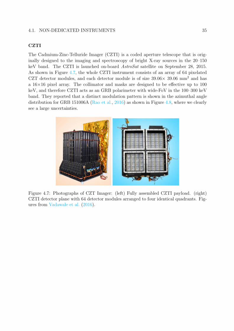
The Cadmium-Zinc-Telluride Imager (CZTI) is a coded aperture telescope that is orig-
inally designed to the imaging and spectroscopy of bright X-ray sources in the 20–150
keV band. The CZTI is launched on-board AstroSat satellite on September 28, 2015.
As shown in Figure 4.7, the whole CZTI instrument consists of an array of 64 pixelated
CZT detector modules, and each detector module is of size 39.06× 39.06 mm2 and has
a 16×16 pixel array. The collimator and masks are designed to be effective up to 100
keV, and therefore CZTI acts as an GRB polarimeter with wide-FoV in the 100–300 keV
band. They reported that a distinct modulation pattern is shown in the azimuthal angle
distribution for GRB 151006A (Rao et al., 2016) as shown in Figure 4.8, where we clearly
see a large uncertainties.
Figure 4.7: Photographs of CZT Imager: (left) Fully assembled CZTI payload. (right)CZTI detector plane with 64 detector modules arranged to four identical quadrants. Fig-ures from Vadawale et al. (2016).

36 4.1. NON-DEDICATED INSTRUMENTS
Figure 4.8: CZTI observation of GRB 151006A. The red solid line is the cos (2ϕ) fit to theazimuthal scattering distribution. The degree of polarization is obtained as ∼0.32 with adetection significance of 1.5σ. The fitted polarization angle is ∼156 in the CZTI plane(Rao et al., 2016).

4.2. POINTING POLARIMETER 37
4.2 Pointing Polarimeter
A pointing observation is a simple solution to constrain the direction of incident photons.
Thanks to their narrow FoV, we do not need to consider the systematic modulations due to
the off-axis incidence. In addition, the non-uniformity of the detector is canceled out when
the detector rotates around its optical axis. Furthermore, on-source/off-source observation
strategy allows an estimation of the background without relying on the simulation, and
enables the subtraction of possible background modulation as mentioned in Section 3.3.
Figure 4.9: Schematic view of the X-Calibur (Kislat et al., 2017).
Figure 4.10: Effective area as function of the photon energy of the X-ray mirror (Guo,2014).
X-Calibur (Beilicke et al., 2014) is a balloon-borne Compton polarimeter combined
with the InFOCuS grazing incidence X-ray mirror (Ogasaka et al., 2005) for the energy
range from 20 to 60 keV. X-rays from a celestial source are focused with the X-ray mirror
and scattered onto a 13 mm-diameter plastic scintillator rod as shown in Figure 4.9.
The scattered X-ray is recorded by an array of Cadmium-Zinc-Telluride (CZT) detectors
surrounding the scattering rod. The focal length of the mirror is 8 m and the field of
view is 8 arcmin at 20 keV. In addition to the background suppression by the active and
passive shielding around the detector, the X-ray mirror collects only photons coming from
the source direction to a small focusing spot area and dramatically improve the statistical
accuracy. The limit of the energy in focusing by reflection is order of 10 keV, and the
effective area of the mirror falls suddenly in the higher energy as shown in Figure 4.10.
The X-Calibur group reported a high modulation factor of 0.5–0.7, which is close to limit
set determined by geometrical configuration of Compton polarimeters. In addition, they
control the systematic modulations through the rotation of detector at 2 rotations per
38 4.2. POINTING POLARIMETER
minute. The calculated MDPs for bright celestial sources, such as Crab nebula, Sco X-1,
and Cyg X-1, are ∼10% for several hours observations in balloon experiment. Although a
one-day balloon-borne experiment was carried out in 2014, no cosmic X-ray sources were
observed due to a failure of the pointing system. They have upgraded X-Calibur and plan
to perform a long-duration balloon flight for the 2018 or 2019 season (Kislat et al., 2017).
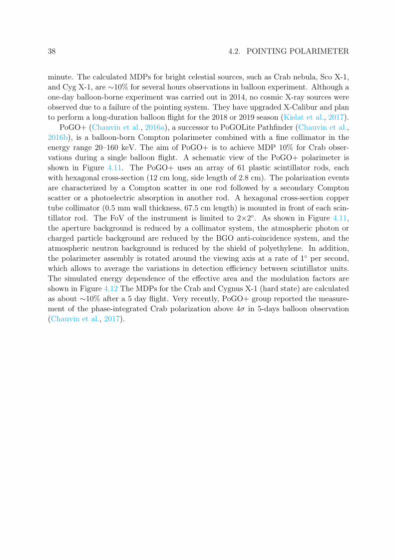
PoGO+ (Chauvin et al., 2016a), a successor to PoGOLite Pathfinder (Chauvin et al.,
2016b), is a balloon-born Compton polarimeter combined with a fine collimator in the
energy range 20–160 keV. The aim of PoGO+ is to achieve MDP 10% for Crab obser-
vations during a single balloon flight. A schematic view of the PoGO+ polarimeter is
shown in Figure 4.11. The PoGO+ uses an array of 61 plastic scintillator rods, each
with hexagonal cross-section (12 cm long, side length of 2.8 cm). The polarization events
are characterized by a Compton scatter in one rod followed by a secondary Compton
scatter or a photoelectric absorption in another rod. A hexagonal cross-section copper
tube collimator (0.5 mm wall thickness, 67.5 cm length) is mounted in front of each scin-
tillator rod. The FoV of the instrument is limited to 2×2. As shown in Figure 4.11,
the aperture background is reduced by a collimator system, the atmospheric photon or
charged particle background are reduced by the BGO anti-coincidence system, and the
atmospheric neutron background is reduced by the shield of polyethylene. In addition,
the polarimeter assembly is rotated around the viewing axis at a rate of 1 per second,
which allows to average the variations in detection efficiency between scintillator units.
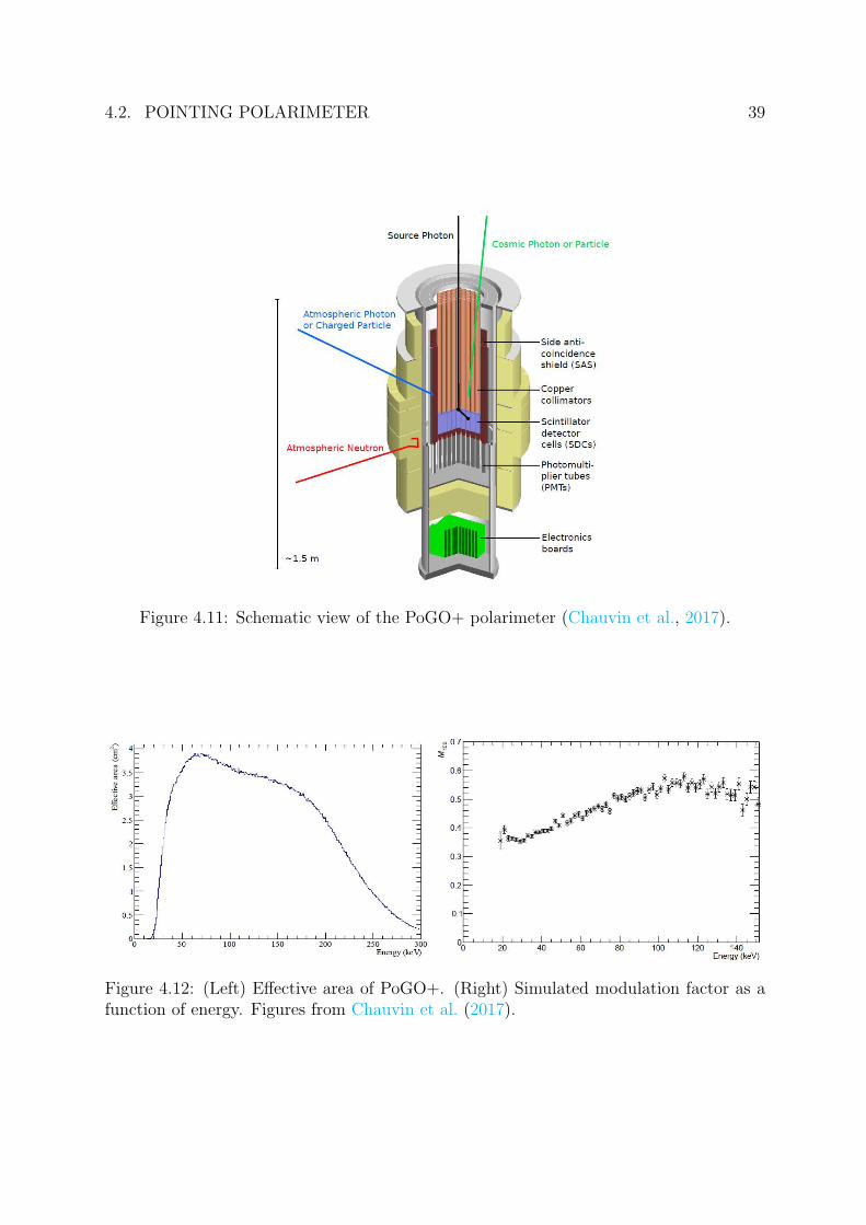
The simulated energy dependence of the effective area and the modulation factors are
shown in Figure 4.12 The MDPs for the Crab and Cygnus X-1 (hard state) are calculated
as about ∼10% after a 5 day flight. Very recently, PoGO+ group reported the measure-
ment of the phase-integrated Crab polarization above 4σ in 5-days balloon observation
(Chauvin et al., 2017).
4.2. POINTING POLARIMETER 39
Figure 4.11: Schematic view of the PoGO+ polarimeter (Chauvin et al., 2017).
Figure 4.12: (Left) Effective area of PoGO+. (Right) Simulated modulation factor as afunction of energy. Figures from Chauvin et al. (2017).
40 4.2. POINTING POLARIMETER
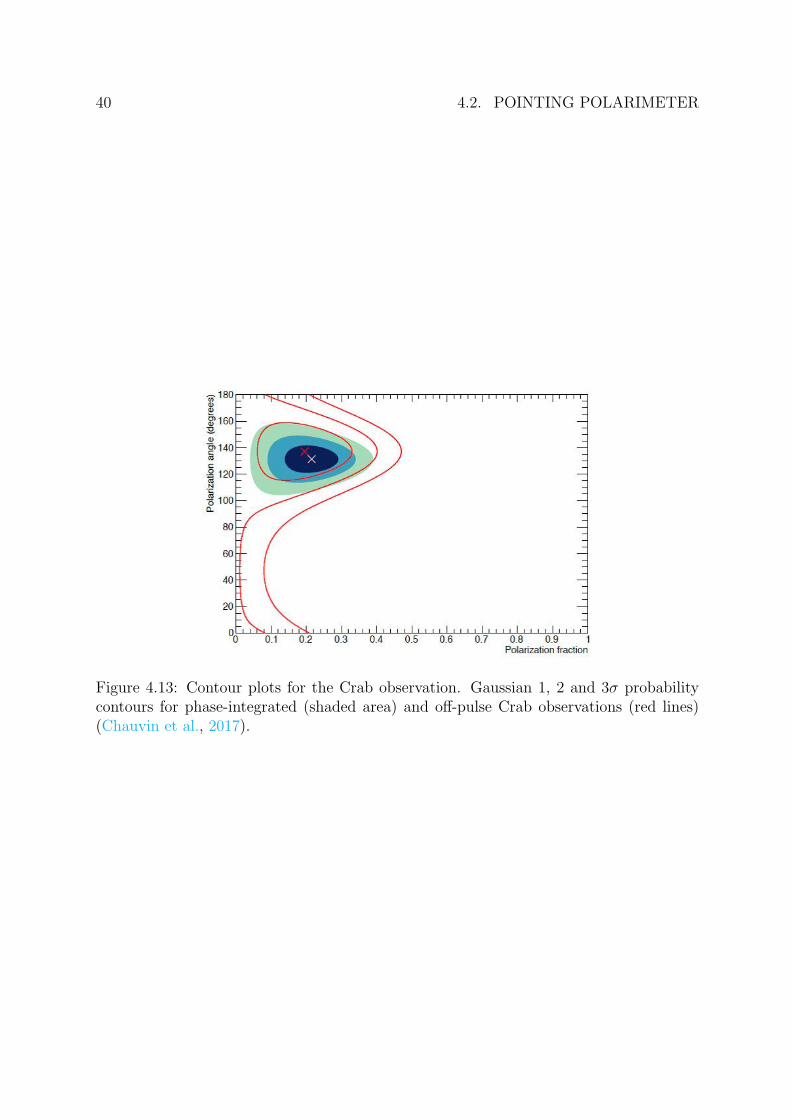
Figure 4.13: Contour plots for the Crab observation. Gaussian 1, 2 and 3σ probabilitycontours for phase-integrated (shaded area) and off-pulse Crab observations (red lines)(Chauvin et al., 2017).
4.3. GRB POLARIMETER 41
4.3 GRB Polarimeter
To observe bright GRBs, several Compton polarimeters with wide FoV and moderate
detection area have been developed. The GAmma-ray Polarimeter (GAP) is the first
flight instruments dedicated to GRB polarization measurements in the energy range 70–
300 keV (Yonetoku et al., 2011a). The GAP experiment was flown as additional part
of a Japanese solar power sail demonstration mission known as IKAROS (Interplane-
tary Kite-craft Accelerated by the Radiation Of the Sun) and performed several GRB
observations in the deep space. As shown in Figure 4.14, it consists of one large plastic
scintillator surrounded by an array of 12 CsI(Tl) scintillators. The location of the hit
CsI detector gives N (ϕdet), however D(θdet, ϕdet) cannot be measured. The effective area
and the modulation factor at 100 keV were 30 cm2 and ∼0.3, respectively. In contrast
to the RHESSI, GAP has a high axial symmetry and a high gain uniformity to suppress
the systematic modulations due to background photons. The GAP group carried out the
ground-based calibration using polarized X-ray beam and confirmed that the simulated
N (ϕdet) is agree well with the measured one in the case of on-axis incident. During two
years observations, the GAP group reported three GRB polarization detections as shown
in Table 2.2 with significance of ∼ 3σ. To determine the measured polarization states,
they simulated the model function of N (ϕdet) with step resolutions of 5% for polarization
degrees and 5 for polarization angles with GEANT4 Monte Carlo simulations. The
measured N (ϕdet), which does not follow cos(2ϕdet), have been fitted using a least-squares
method to the modeled modulation curves directly. The right of Figure 4.15 shows the
measured and best fitted modulation curves, which represents the change of polarization
angle during the interval of prompt emission of GRB 100826A, which was located at 20.0
off-axis from the center of the GAP field of view. We note that GRB 100826A was very
bright burst with the energy fluence of ∼3.0×10⁻⁴ erg cm−2, which happen ∼1 events per
year in the whole sky. Even in this case, the signal-to-noise ratio estimated from Figure
4.15 is not large, ∼1 on Interval-1 and ∼0.3 on Interval-2.
There has been proposals of various GRB polarimeters with wide-FoV and simple
geometries consisting of an array of pixelated plastic scintillators so far (Bloser et al., 2009;
Yonetoku et al., 2011a; Gunji et al., 2014; Yatsu et al., 2014). In particular, POLAR
has recently launched on-board the Chinese space laboratory Tiangong-2 in 2016. The
POLAR detector consists of an array of 5 × 5 modules, each of which includes 8 × 8
plastic scintillator bars as shown in Figure 4.16. Both the Compton scattering interaction
of the photon and its secondary interaction, photoabsorption, are measured using the
scintillator bars. The POLAR detector aims to measure the polarization of the prompt
emission from GRBs in the 50–500 keV energy range with the wide FoV of about π str. It
has been estimated that MDPs for bright GRB with a 10−5 erg cm2 fluence are about 10%
and therefore POLAR would measure the polarization of 10 GRBs with 10% polarization
during a one-year observation at least. POLAR group reported that about 50 GRBs are
detected within 6 months, and the polarization analysis of those GRBs are underway

42 4.3. GRB POLARIMETER
R6041
Super Bialkali
R7400-06
HV unit (CsI) HV unit (Plastic)
Analog
FPGACPU
Plastic ScintillatorCsI
5mm
60m
m
140mm
Lead 0
.3m
m thic
kness
160m
m
170mm
Lead 0
.5m
m
thic
kness
Lead 0.5mm thickness
Figure 4.14: Schematic view of the GAP detector (Yonetoku et al., 2011a).
(http://polar.psi.ch/pub/).
These wide-FoV GRB polarimeters have four problems that should be noted. Due
to the lack of imaging capabilities, (1) they are not able to confirm the reliability of the
simulation in space by measuring the unpolarized background as mentioned in Section
3.2.2; (2) the MDP is statistically degraded by a huge background contribution coming
from all directions as mentioned in Section 3.3; (3) they essentially have to rely on other
satellites to know the direction of the target sources, which would reduce the number of
GRBs to be measured. In addition, due to the lack of measurement of θdet, (4) they are
not able to correct the off-axis incident effect, and the MDP is also degraded by increasing
the incident angle as mentioned in Section 3.2.3.
The bright GRBs with the fluence of larger than 10−5 erg cm−2 happen ∼50 events
per year in the whole sky. Therefore, the GRBs located in the 2π-steradian-FoV, which
should be observed by other satellites simultaneously, are reduced to ∼10 events per year.
The number of GRBs which have a degree of polarization larger than the degraded MDP,
is further reduced to several events per year, which is fewer than are necessary for the
statistical analysis of GRB polarizations as mentioned in Section 2.2.1.
4.3. GRB POLARIMETER 43
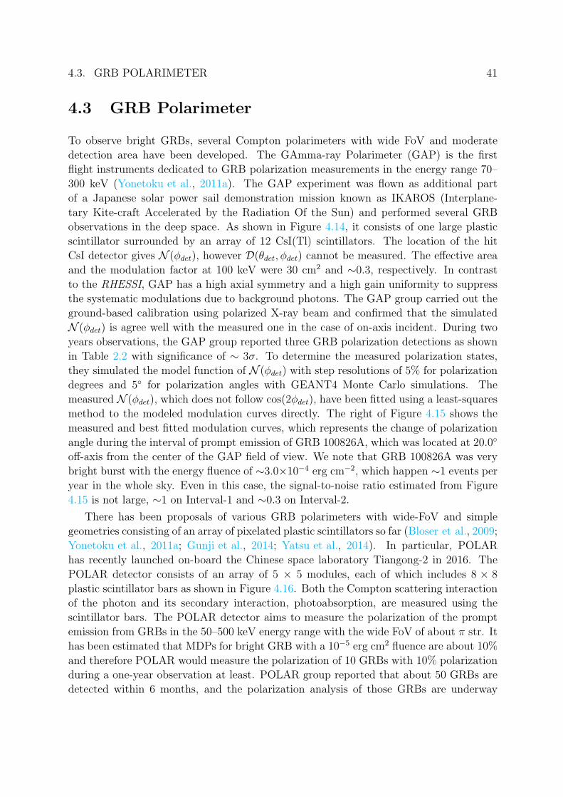
Figure 4.15: (Left) Light curve of the prompt gamma-ray emission of GRB100826A de-tected by the GAP. The GAP group divided the data into Interval-1 and -2 for thepolarization analysis. (Right) Number of coincidence gamma-ray photons against thescattering angle of GRB 100826A measured by the GAP in 70–300 keV band. Blackfilled and open squares are the angular distributions of Compton scattered gamma-raysof Interval-1 and -2, respectively. The gray solid lines are the best-fit models calculatedby the Geant4 Monte Carlo simulations (Yonetoku et al., 2011b).
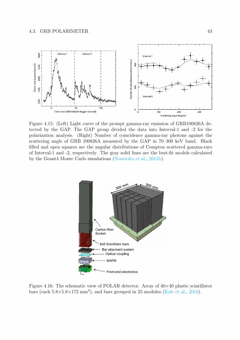
Figure 4.16: The schematic view of POLAR detector. Array of 40×40 plastic scintillatorbars (each 5.8×5.8×172 mm3), and bars grouped in 25 modules (Kole et al., 2016).
44 4.4. COMPTON CAMERA
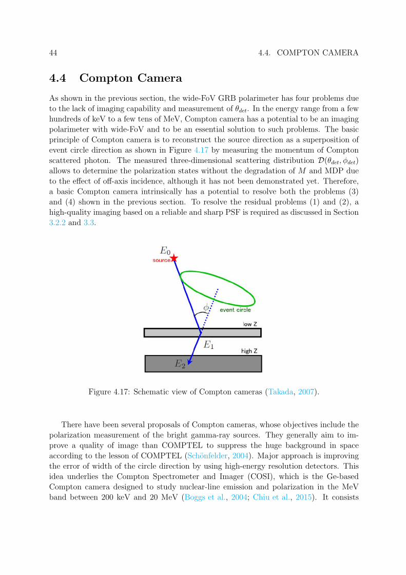
4.4 Compton Camera
As shown in the previous section, the wide-FoV GRB polarimeter has four problems due
to the lack of imaging capability and measurement of θdet. In the energy range from a few
hundreds of keV to a few tens of MeV, Compton camera has a potential to be an imaging
polarimeter with wide-FoV and to be an essential solution to such problems. The basic
principle of Compton camera is to reconstruct the source direction as a superposition of
event circle direction as shown in Figure 4.17 by measuring the momentum of Compton
scattered photon. The measured three-dimensional scattering distribution D(θdet, ϕdet)
allows to determine the polarization states without the degradation of M and MDP due
to the effect of off-axis incidence, although it has not been demonstrated yet. Therefore,
a basic Compton camera intrinsically has a potential to resolve both the problems (3)
and (4) shown in the previous section. To resolve the residual problems (1) and (2), a
high-quality imaging based on a reliable and sharp PSF is required as discussed in Section
3.2.2 and 3.3.
Figure 4.17: Schematic view of Compton cameras (Takada, 2007).
There have been several proposals of Compton cameras, whose objectives include the
polarization measurement of the bright gamma-ray sources. They generally aim to im-
prove a quality of image than COMPTEL to suppress the huge background in space
according to the lesson of COMPTEL (Schonfelder, 2004). Major approach is improving
the error of width of the circle direction by using high-energy resolution detectors. This
idea underlies the Compton Spectrometer and Imager (COSI), which is the Ge-based
Compton camera designed to study nuclear-line emission and polarization in the MeV
band between 200 keV and 20 MeV (Boggs et al., 2004; Chiu et al., 2015). It consists
4.4. COMPTON CAMERA 45
of ten high-purity germanium crossedstrip detectors that work as the both scatterer and
absorber, enable the measurement of the three-dimensional points of the scattering and
absorption point, as shown in Figure 4.18. The COSI has an active shield made of BGO
scintillator, and the field of view is constrained to be 3.2 sr. Very recently, they suc-
ceeded to obtain the gamma-ray images of a few celestial objects and transients including
one GRB in the long-duration balloon experiment (Kierans et al., 2017), however they
reported that the MDP in this burst was very large ∼60–70% and COSI did not detect
the polarization (Lowell et al., 2017).
Another promising approach is to determine the direction of the incident photon event
by event, not circle direction, by measuring the initial direction of the Compton recoil
electron, which surely change the imaging quality dramatically. Importantly, as pointed
out in (Tanimori et al., 2015), the precise measurement of electron tracks achieve a proper
geometrical imaging with well-defined PSF, which enables us to perform an accurate
imaging spectroscopic measurement as same as optical, X-ray and GeV telescopes . Many
groups have proposed and studied the Compton camera with an electron tracker using
the stacked solid-state detectors, which is designed to measure the recoil electron with an
energy of more than a few MeV (O’Neill et al., 1996; Bloser et al., 2002; Kurfess et al.,
2004; Moiseev et al., 2015; Khalil et al., 2016; Tatischeff et al., 2016). On these types of
Compton cameras, only the Medium Energy Gamma-Ray Astronomy telescope (MEGA;
see Figure 4.19) succeeded the demonstration of gamma-ray imaging polarimetry for on-
axis incidence of 100% polarized pencil beams at different energies (0.7, 2, and 5 MeV)
(Zoglauer et al., 2004), where the beam images were reconstructed without (at 0.7 and 2
MeV) and with (at 5 MeV) electron tracks (Andritschke et al., 2005). Unfortunately, such
a solid state electron tracker provided too sparse tracking to create an idea of well-defined
PSF in Compton scattering. A fine electron tracking enough to define a PSF is realized
only by an Electron-Tracking Compton Camera (ETCC) with a gaseous electron tracker
as discussed in the next chapter.

46 4.4. COMPTON CAMERA
Figure 4.18: Schematic view of COSI detector (Chiu et al., 2015).
Figure 4.19: Schematic view of MEGA detector (Kanbach et al., 2003).
Chapter 5
Electron-Tracking Compton Camera
We have developed an electron-tracking Compton camera (ETCC) utilizing a gaseous
three-dimensional electron tracker since 2004 (Tanimori et al., 2004). The gaseous tracker
enables us to measure a quite fine three dimensional tracks as seen in a cloud chamber,
while solid state trackers provide only several hit points for a track. Such fine electron
tracking at first enables us to define a well-defined PSF, and thus consequently the de-
tection and polarization sensitivity are greatly improved.
To verify the polarimetric performance of the ETCC, we used the ETCC with 30-
cm cubic gaseous electron tracker, which has been originally developed since 2013 to
measure the sub-MeV gamma-ray spectrum of the Crab with 6 hours balloon flight
(Tanimori et al., 2015). Here we overview the detector configuration and the basic per-
formance of the ETCC, which will be used in the polarimetric simulation and experiment
in the following chapters.
5.1 Advantages of Electron Tracking
An Electron-Tracking Compton Camera (ETCC) reconstructs the both incident direction
and energy of the gamma ray by measuring the momenta of the scattering gamma ray and
recoil electron. The reconstructed energy E0 and unit vector of the momentum direction
srcs are expressed as
E0 = Eγ +Ke, (5.1)
srcs =
(cosϕ− sinϕ
tanα
)g +
sinϕ
sinαe
=Eγ
Eγ +Ke
g +
√Ke(Ke + 2mec2)
Eγ +Ke
e, (5.2)
(5.3)
47

48 5.1. ADVANTAGES OF ELECTRON TRACKING
Figure 5.1: Schematic of an Electron-Tracking Compton Camera. It consists of an elec-tron tracker as the scatterer made of low-Z material and an absorber made of high-Zmaterial. The scatterer measures the scattering position x1, and the kinematic energyand momentum unit vector of the recoil electron, e and Ke, respectively. The absorbermeasures the absorption position x2 and energy of the scattered gamma ray Eγ. The mo-mentum unit vector of the scattered gamma ray is obtained by calculating (x2 - x1)/|x2
- x1| Figure from Sawano (2017).
where Eγ and Ke, and g and e are the kinetic energies and unit vectors of momentum
directions of the scattering gamma ray and the Compton-recoil electron, respectively, ϕ
is the polar scattering angle of the gamma ray, and α is the angle between the g and e as
shown in Figure 5.1.
The primary advantage of electron tracking is the realization of the PSF based on ge-
ometrical optics, where there has been no definition of two dimensional PSF in Compton
cameras. There are two components of the PSF. One is the uncertainty of the scattering
angle ϕ, referred as the angular resolution measure (ARM), and the other is of the scat-
tering plane of the gamma ray, referred as the scattering plane deviation (SPD) as shown
in Figure 5.1. The errors of the reconstructed direction concerning the ARM and SPD,
∆ϕARM and ∆ϕSPD are derived by
∆ϕARM = arccos (s · g)− arccos
(1− mec
2
Eγ +Ke
Ke
Eγ
), (5.4)
∆ϕSPD = sign
(g ·
(s× g
|s× g|× srcs × g
| srcs × g|
))arccos
(s× g
|s× g|· srcs × g
| srcs × g|
), (5.5)
5.1. ADVANTAGES OF ELECTRON TRACKING 49
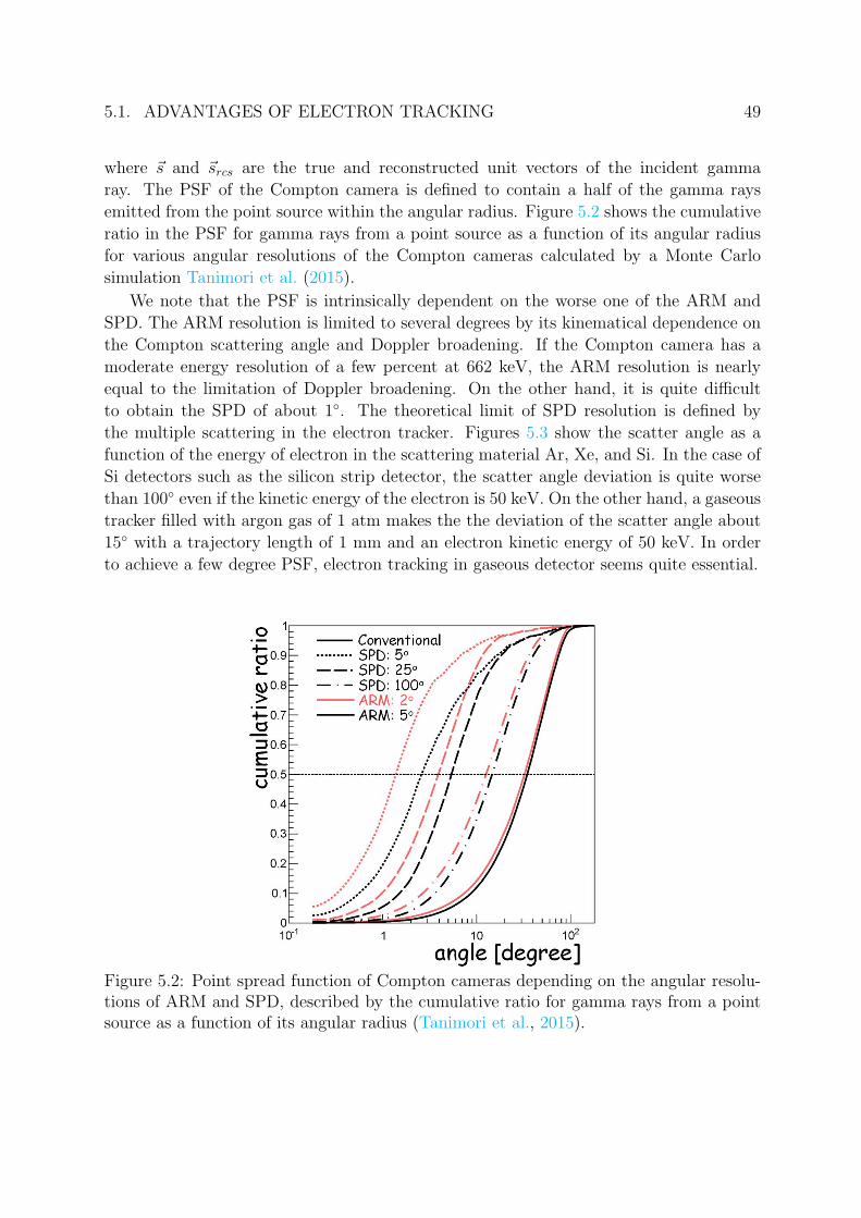
where s and srcs are the true and reconstructed unit vectors of the incident gamma
ray. The PSF of the Compton camera is defined to contain a half of the gamma rays
emitted from the point source within the angular radius. Figure 5.2 shows the cumulative
ratio in the PSF for gamma rays from a point source as a function of its angular radius
for various angular resolutions of the Compton cameras calculated by a Monte Carlo
simulation Tanimori et al. (2015).
We note that the PSF is intrinsically dependent on the worse one of the ARM and
SPD. The ARM resolution is limited to several degrees by its kinematical dependence on
the Compton scattering angle and Doppler broadening. If the Compton camera has a
moderate energy resolution of a few percent at 662 keV, the ARM resolution is nearly
equal to the limitation of Doppler broadening. On the other hand, it is quite difficult
to obtain the SPD of about 1. The theoretical limit of SPD resolution is defined by
the multiple scattering in the electron tracker. Figures 5.3 show the scatter angle as a
function of the energy of electron in the scattering material Ar, Xe, and Si. In the case of
Si detectors such as the silicon strip detector, the scatter angle deviation is quite worse
than 100 even if the kinetic energy of the electron is 50 keV. On the other hand, a gaseous
tracker filled with argon gas of 1 atm makes the the deviation of the scatter angle about
15 with a trajectory length of 1 mm and an electron kinetic energy of 50 keV. In order
to achieve a few degree PSF, electron tracking in gaseous detector seems quite essential.
Figure 5.2: Point spread function of Compton cameras depending on the angular resolu-tions of ARM and SPD, described by the cumulative ratio for gamma rays from a pointsource as a function of its angular radius (Tanimori et al., 2015).

50 5.2. DETECTOR CONFIGURATION
energy [keV]0 50 100 150 200 250 300 350 400 450 500
[d
egre
e]rm
sθ
0
10
20
30
40
50
60
70
80
90
500µm
Si
Xe 1atm
Ar 2atmAr 1atm
energy [keV]0 50 100 150 200 250 300 350 400 450 500
[d
egre
e]rm
sθ
0
10
20
30
40
50
60
70
80
90
1mm
Xe 1atm
Ar 2atmAr 1atm
energy [keV]0 50 100 150 200 250 300 350 400 450 500
[d
egre
e]rm
sθ
0
10
20
30
40
50
60
70
80
90
5mm
Xe 1atmAr 2atm
Ar 1atm
Figure 5.3: Scatter angle deviation with different ranges of the electron (left: 500µm,middle: 1mm, right: 5mm; temperature: 20C; Takada 2007).
The information of an electron track also gives us the tools to suppress various back-
grounds. The angle α (see Figure 5.1) is obtained by two independent ways. One is
geometrically, calculating the inner product of the recoil electron vector and the scattered
gamma-ray vector. The other is kinematically, calculating based on Compton kinematics
with the measured energy deposit in TPC and PSAs. By checking the consistency be-
tween these two values, an ETCC rejects Compton scattering fake events such as chance
coincidence hits of the TPC and PSAs and events where Compton scattering occurred
in the PSAs. We can also obtain the energy-loss rate (dE/dx) of charged particles inter-
acted in TPC by using the relationship of its energy and range calculated from the track
information. Therefore, we can identify the kind of particles and reject non gamma-ray
backgrounds, such as cosmic rays, neutrons and Compton-recoil electrons escaping from
TPC. Thanks to these background suppression tools, without an active veto shielding,
ETCC also has the large Field of View (FoV).
5.2 Detector Configuration
Figure 5.4 shows a schematic view and a photograph of the ETCC. Gd2SiO5:Ce (GSO)
pixel scintillator arrays (PSAs), which act as absorbers for scattered gamma-rays, are
set under the bottom and at each side of the 30 cm cubic TPC, which is filled with an
Ar-based gas.

5.2. DETECTOR CONFIGURATION 51
Figure 5.4: (a) Schematic view of the ETCC, which consists of a 30 cm-cubic gaseoustime projection chamber (TPC) and pixel scintillator arrays (PSAs). The TPC detectsthe track and energy of the recoil electron, and the PSAs detect the pixel position of theabsorption and the energy of the scattered gamma-rays event by event (Tanimori et al.,2015).

52 5.2. DETECTOR CONFIGURATION
5.2.1 Gaseous Electron Tracker
Figure 5.5: Schematic view of the gaseous electron tracker of the ETCC.
As shown in Figure 5.5, the gaseous electron tracker consists of a micro pattern
gas detector (µ-PIC; Ochi et al., 2002), a gas electron multiplier (GEM; Sauli, 1997;
Tamagawa et al., 2006), and a 312-mm thick gas detection volume. A brief explana-
tion of a µ-PIC and a GEM is given in the caption of Figures 5.6 and 5.7, respectively.
The µ-PIC in the gaseous electron tracker has an effective area of 307.2 × 307.2 mm2
and 768 × 768 pixels with a pitch of 400 µm, which are connected orthogonally by 768
anode strips and 768 cathode strips (Takada et al., 2007). GEM with an effective area of
320 × 320 mm2 is placed 5 mm above the µ-PIC as a sub-amplifier. GEM is made of a
100 µm-thick liquid crystal polymer, and the hole size and pitch are 70 µm and 140 µm,
respectively. The combination of the µ-PIC and the GEM is used as a time projection
chamber (TPC), where the electric drift field is applied to the detection volume and the
drift time for which the electrons reach to the detector X–Y plane is used for the deter-
mination of the position along to the Z-axis. The filling gas of the TPC is a mixtured
gas of (Ar 95%, CF4 3%, iso-C4H10 2%) with 1 atm, and the gas gains of the µ-PIC and
GEM are 2000 and 10, respectively.
We used the TPC readout board (Mizumoto et al., 2015) to read the µ-PIC signals.
The TPC readout board contains 4 flash ADCs, an Ethernet port, an FPGA, and 8 CMOS
FE2009bal ASIC chips, as shown in Figure 5.8. All discriminated signals from 128 input
channels are fed to the FPGA. In the FPGA, the hit patterns and timing of the anode or
cathode electrodes are individually synchronized with 100MHz (10 ns) clocks and recorded
to the memory module in the VME bus. The three-dimensional hit position in the TPC
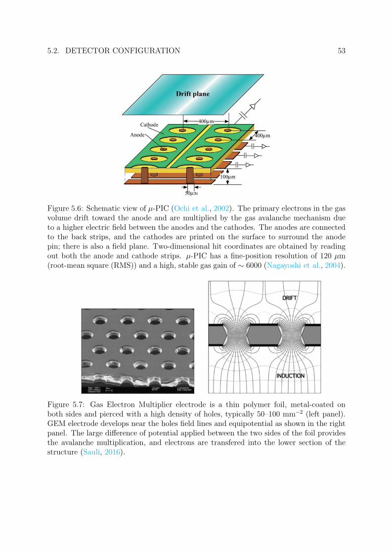
5.2. DETECTOR CONFIGURATION 53
Figure 5.6: Schematic view of µ-PIC (Ochi et al., 2002). The primary electrons in the gasvolume drift toward the anode and are multiplied by the gas avalanche mechanism dueto a higher electric field between the anodes and the cathodes. The anodes are connectedto the back strips, and the cathodes are printed on the surface to surround the anodepin; there is also a field plane. Two-dimensional hit coordinates are obtained by readingout both the anode and cathode strips. µ-PIC has a fine-position resolution of 120 µm(root-mean square (RMS)) and a high, stable gas gain of ∼ 6000 (Nagayoshi et al., 2004).
Figure 5.7: Gas Electron Multiplier electrode is a thin polymer foil, metal-coated onboth sides and pierced with a high density of holes, typically 50–100 mm−2 (left panel).GEM electrode develops near the holes field lines and equipotential as shown in the rightpanel. The large difference of potential applied between the two sides of the foil providesthe avalanche multiplication, and electrons are transfered into the lower section of thestructure (Sauli, 2016).
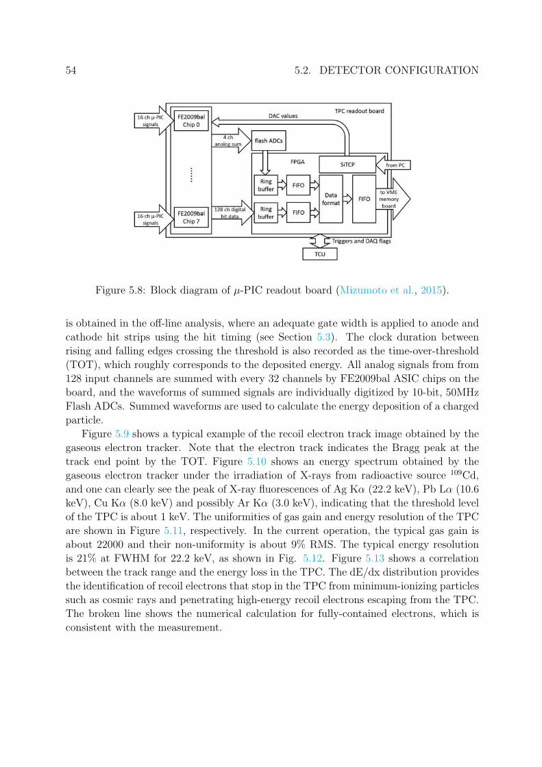
54 5.2. DETECTOR CONFIGURATION
Figure 5.8: Block diagram of µ-PIC readout board (Mizumoto et al., 2015).
is obtained in the off-line analysis, where an adequate gate width is applied to anode and
cathode hit strips using the hit timing (see Section 5.3). The clock duration between
rising and falling edges crossing the threshold is also recorded as the time-over-threshold
(TOT), which roughly corresponds to the deposited energy. All analog signals from from
128 input channels are summed with every 32 channels by FE2009bal ASIC chips on the
board, and the waveforms of summed signals are individually digitized by 10-bit, 50MHz
Flash ADCs. Summed waveforms are used to calculate the energy deposition of a charged
particle.
Figure 5.9 shows a typical example of the recoil electron track image obtained by the
gaseous electron tracker. Note that the electron track indicates the Bragg peak at the
track end point by the TOT. Figure 5.10 shows an energy spectrum obtained by the
gaseous electron tracker under the irradiation of X-rays from radioactive source 109Cd,
and one can clearly see the peak of X-ray fluorescences of Ag Kα (22.2 keV), Pb Lα (10.6
keV), Cu Kα (8.0 keV) and possibly Ar Kα (3.0 keV), indicating that the threshold level
of the TPC is about 1 keV. The uniformities of gas gain and energy resolution of the TPC
are shown in Figure 5.11, respectively. In the current operation, the typical gas gain is
about 22000 and their non-uniformity is about 9% RMS. The typical energy resolution
is 21% at FWHM for 22.2 keV, as shown in Fig. 5.12. Figure 5.13 shows a correlation
between the track range and the energy loss in the TPC. The dE/dx distribution provides
the identification of recoil electrons that stop in the TPC from minimum-ionizing particles
such as cosmic rays and penetrating high-energy recoil electrons escaping from the TPC.
The broken line shows the numerical calculation for fully-contained electrons, which is
consistent with the measurement.

5.2. DETECTOR CONFIGURATION 55
Figure 5.9: Typical examples of the projected track of a recoil electron, where both hitpoints are depicted. Since the drift velocity is 8 cm/µsec, 1 clock corresponds to 0.8mm.In addition, the clock duration between rising and falling edges crossing the threshold isrecorded as the time-over-threshold (TOT), which roughly corresponds to the depositedenergy (Mizumoto et al., 2015).
Energy (keV)
0 10 20 30
Cou
nts
(arb
. uni
t)
0
500
1000
Figure 5.10: Spectrum obtained by irradiation of radioactive isotope source of 109Cd.photoelectric peaks can be seen at Ag Kα (22.2 keV) from 109Cd, and Pb Lα (10.6 keV),Cu Kα (8.0 keV) and possibly Ar Kα (3.0 keV) from the materials that are used for theTPC (Sawano, 2017).

56 5.2. DETECTOR CONFIGURATION
Anode0
5
10Cathode
0
5
10
Rel
ativ
e ga
s ga
in
0.6
0.8
1
1.2
1.4
0.6
0.8
1
1.2
1.4
Figure 5.11: Gas gain map of the TPC. Colormaps represent the relative gas gain with re-spect to the mean gas gain of the whole re-gion (Sawano, 2017).
Anode0
24
68
10Cathode0
24
68
10
Ene
rgy
reso
lutio
n (%
)
10
15
20
25
30
35
40
10
15
20
25
30
35
40
Figure 5.12: Distribution of the energy res-olution for Ag Kα (22.2 keV). The meanenergy resolution is about 21% (FWHM)(Sawano, 2017).
Figure 5.13: Track range vs the energy loss in the TPC under the condition of gamma-rayirradiation from 137Cs (3 MBq) at a distance of 1 m in the laboratory (Tanimori et al.,2015). The broken solid line represents the numerical calculation curves of the energy lossfor fully-contained electrons.
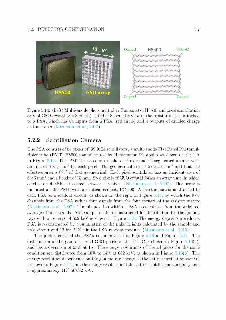
5.2. DETECTOR CONFIGURATION 57
Figure 5.14: (Left) Multi-anode photomultiplier Hamamatsu H8500 and pixel scintillationarry of GSO crystal (8×8 pixels). (Right) Schematic view of the resistor matrix attachedto a PSA, which has 64 inputs from a PSA (red circle) and 4 outputs of divided chargeat the corner (Mizumoto et al., 2015).
5.2.2 Scintillation Camera
The PSA consists of 64 pixels of GSO:Ce scntillators, a multi-anode Flat Panel Photomul-
tipier tube (PMT) H8500 manufactured by Hamamatsu Photonics as shown on the left
in Figure 5.14. This PMT has a common photocathode and 64-segmented anodes with
an area of 6 × 6 mm2 for each pixel. The geometrical area is 52 × 52 mm2 and thus the
effective area is 89% of that geometrical. Each pixel scintillator has an incident area of
6×6 mm2 and a height of 13 mm. 8×8 pixels of GSO crystal forms an array unit, in which
a reflector of ESR is inserted between the pixels (Nishimura et al., 2007). This array is
mounted on the PMT with an optical cement, BC-600. A resistor matrix is attached to
each PSA as a readout circuit, as shown on the right in Figure 5.14, by which the 8×8
channels from the PSA reduce four signals from the four corners of the resistor matrix
(Nishimura et al., 2007). The hit position within a PSA is calculated from the weighted
average of four signals. An example of the reconstructed hit distribution for the gamma
rays with an energy of 662 keV is shown in Figure 5.15. The energy deposition within a
PSA is reconstructed by a summation of the pulse heights calculated by the sample and
hold circuit and 12-bit ADCs in the PSA readout modules (Mizumoto et al., 2015).
The performance of the PSAs is summarized in Figure 5.16 and Figure 5.17. The
distribution of the gain of the all GSO pixels in the ETCC is shown in Figure 5.16(a),
and has a deviation of 25% at 1σ. The energy resolutions of the all pixels for the same
condition are distributed from 10% to 14% at 662 keV, as shown in Figure 5.16(b). The
energy resolution dependence on the gamma-ray energy as the entire scintillation camera
is shown in Figure 5.17, and the energy resolution of the entire scintillation camera system
is approximately 11% at 662 keV.

58 5.2. DETECTOR CONFIGURATION
x [a.u.]0.25− 0.2− 0.15− 0.1− 0.05− 0 0.05 0.1 0.15 0.2 0.25
y [a
.u.]
0.5−
0.4−
0.3−
0.2−
0.1−
0
0.1
0.2
0.3
0.4
0.5
1
10
210
310
Figure 5.15: Reconstructed hit distribution image of the one unit of the PSA for thegamma rays with an energy of 662 keV (Mizumoto et al., 2015).
gain (ADC value/keV)0 1 2 3 4 5 6 7 8 9 10
num
ber
of p
ixel
s
0
50
100
150
200
250
300
350
energy resolution [%] (for 662 keV)0 5 10 15 20 25 30
num
ber
of p
ixel
s
0
20
40
60
80
100
120
140
160
180
200
220
Figure 5.16: (Left) Gain distribution of the whole channels of the scintillation camera.The unit of the gain is ADU/keV and divided by the average. (Right) the same but forthe energy resolution at FWHM for 662 keV (Mizumoto et al., 2015).

5.2. DETECTOR CONFIGURATION 59
energy [keV]
210 310
ener
gy r
esol
utio
n [%
]
10
Figure 5.17: Energy resolution of the entire scintillation camera as a function of theincident gamma-ray energy (Mizumoto et al., 2015).

60 5.3. EVENT RECONSTRUCTION
5.3 Event Reconstruction
Events are taken with a coincidence between the TPC and PSAs in the ETCC. There
exists, however, lots of background events such as random coincidence events, charged
particles such as cosmic muons, environmental gamma rays, and incomplete events, in
which a electron penetrates from the gas volume or coming from the outside of the gas
volume. To find correct events in which Compton scattering occurs in the active volume
of the TPC and a electron stops within that active volume with one hit in PSAs, we
performed a couple of following selection criteria.
1. Energy loss rate cut
Energy loss rates (or, stopping power) varies depending on β, or the velocity of the
particle. For the electrons in the argon gas with an energy up to a few hundred keV,
the practical range Rp is approximately described as Rp = 0.71(
E1 MeV
)1.72g cm−2,
where E is the energy of the electron (Sauli, 1977). To reject the high energy
electrons escaping from the active volume of the TPC or heavy ions, energy loss
rate cut is applied as follows,Rp ≤ (1/ρ)0.71× E1.72+au
e + bu
Rp ≥ (1/ρ)0.71× E1.72+ale + bl
Rp < Rlimp
, (5.6)
where Ee is the energy loss in the TPC, ρ is the density of the gas of the TPC,
and the Rp is the practical range of the charged particle trajectory in the TPC,
again. au, bu, al, bl, and Rlimp are constants for the event selection. The range Rp is
derived by calculating the length of the diagonal of the rectangular that surrounds
the three-dimensional particle trajectory, formally described as
Rp =√
(xmax − xmin)2 + (ymax − ymin)2 + (min(zx,max, zy,max)−max(zx,min, zy,min))2
(5.7)
where xmax and xmin are the maximum and minimum position coordinates in the
cathode hits, respectively, ymax and ymin are the same but for the anode hits, zx,max
and zy,max are the maximum position coordinates of the hits in the drift direction
for cathode and anode strip data, respectively, and zx,min and zy,min are the same
but for the minimum position coordinates.
2. Fiducial volume cut
Charged particles coming from the outside of the active volume of the TPC cannot
be measured the total kinetic energy properly. To remove such events, the events for
which there are hits near the edge of the active volume in the TPC are considered
as bad events transporting the boundary of the active volume.

5.4. BASIC PERFORMANCES 61
3. Total energy loss cut
For the calibration source, the incident energy of the gamma rays is already-known.
To test the detection efficiency of the gamma rays from radioisotopes, we lay down
the condition where the summation of the energy losses in the TPC and PSA should
be equal to the incident gamma-ray energy, or∣∣∣∣Etpc + Epsa
Einc
− 1
∣∣∣∣ ≤ p, (5.8)
where Etpc, Epsa and Einc are the energy losses in the TPC and PSA, respectively,
and the incident energy, and the p is the fraction of acceptable residual.
Determination of the direction of the recoil electron
To determine the coordinate of the absorption point in the PSA, the scintillator pixel is
firstly identified in the butterfly image, and then the coordinate of the center of the pixel is
regarded as the absorption point. The Compton-scattering points and the direction of the
recoil electrons are determined by the two sets of the two-dimensional hit images whose
space are the clock of the TPC (Z-axis) versus the position number of the µ−PIC strip (X-
axis for cathode and Y -axis for anode). First, the three-dimensional track is reconstructed
by the off-line coincidence of the X–Z and Y –Z images in the three-dimensional space.
Next, the projection to the X–Y plane is made from the three-dimensional track. We
consider that the scattering point projected to the X–Y plane must be located at the
closest hit point from the absorption point (Komura et al., 2013). We also consider that
the Z-coordinate of the scattering point corresponds to the mean of the hits satisfying the
condition on the X–Y projected plane. The direction of the recoil electron is determined
as a composite sum of two vectors of the gradients of the obtained two-dimensional hit
images of X–Z and Y –Z planes.
5.4 Basic Performances
We checked the performance of the ETCC by using the radioisotopes (RIs), 139Ce (166
keV) , 133Ba (356 keV), 22Na (511 keV), 137Cs (662 keV) and 54Mn (835 keV), placed
approximately 2 m from the detector. Figure 5.18 shows the energy resolution of the
ETCC, and its dependence on the incident gamma-ray energy is described as
∆E
E= 10.7×
(E
662 keV
)−0.5
[%] (FWHM). (5.9)
The effective area is calculated by counting the events under the condition where the
total energy loss is consistent within the twice FWHM of the energy resolution from the
incident gamma-ray energy. Figure 5.19 shows the on-axis effective area of the ETCC with
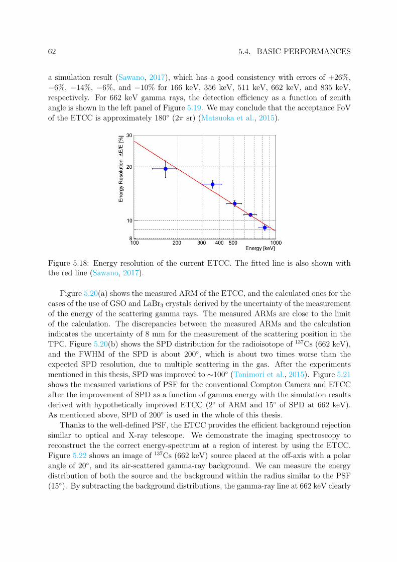
62 5.4. BASIC PERFORMANCES
a simulation result (Sawano, 2017), which has a good consistency with errors of +26%,
−6%, −14%, −6%, and −10% for 166 keV, 356 keV, 511 keV, 662 keV, and 835 keV,
respectively. For 662 keV gamma rays, the detection efficiency as a function of zenith
angle is shown in the left panel of Figure 5.19. We may conclude that the acceptance FoV
of the ETCC is approximately 180 (2π sr) (Matsuoka et al., 2015).
Figure 5.18: Energy resolution of the current ETCC. The fitted line is also shown withthe red line (Sawano, 2017).
Figure 5.20(a) shows the measured ARM of the ETCC, and the calculated ones for the
cases of the use of GSO and LaBr3 crystals derived by the uncertainty of the measurement
of the energy of the scattering gamma rays. The measured ARMs are close to the limit
of the calculation. The discrepancies between the measured ARMs and the calculation
indicates the uncertainty of 8 mm for the measurement of the scattering position in the
TPC. Figure 5.20(b) shows the SPD distribution for the radioisotope of 137Cs (662 keV),
and the FWHM of the SPD is about 200, which is about two times worse than the
expected SPD resolution, due to multiple scattering in the gas. After the experiments
mentioned in this thesis, SPD was improved to ∼100 (Tanimori et al., 2015). Figure 5.21
shows the measured variations of PSF for the conventional Compton Camera and ETCC
after the improvement of SPD as a function of gamma energy with the simulation results
derived with hypothetically improved ETCC (2 of ARM and 15 of SPD at 662 keV).
As mentioned above, SPD of 200 is used in the whole of this thesis.
Thanks to the well-defined PSF, the ETCC provides the efficient background rejection
similar to optical and X-ray telescope. We demonstrate the imaging spectroscopy to
reconstruct the the correct energy-spectrum at a region of interest by using the ETCC.
Figure 5.22 shows an image of 137Cs (662 keV) source placed at the off-axis with a polar
angle of 20, and its air-scattered gamma-ray background. We can measure the energy
distribution of both the source and the background within the radius similar to the PSF
(15). By subtracting the background distributions, the gamma-ray line at 662 keV clearly
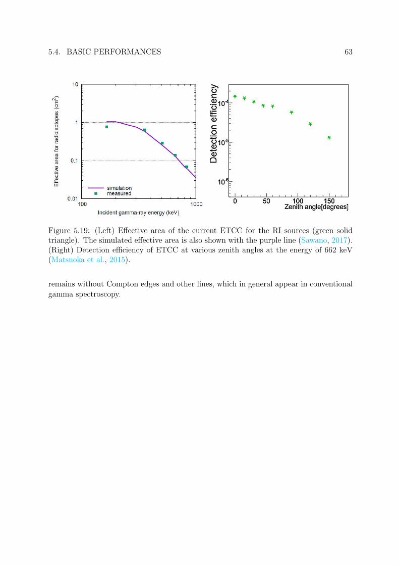
5.4. BASIC PERFORMANCES 63
Figure 5.19: (Left) Effective area of the current ETCC for the RI sources (green solidtriangle). The simulated effective area is also shown with the purple line (Sawano, 2017).(Right) Detection efficiency of ETCC at various zenith angles at the energy of 662 keV(Matsuoka et al., 2015).
remains without Compton edges and other lines, which in general appear in conventional
gamma spectroscopy.
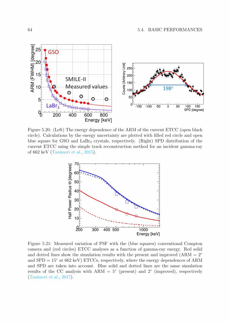
64 5.4. BASIC PERFORMANCES
Figure 5.20: (Left) The energy dependence of the ARM of the current ETCC (open blackcircle). Calculations by the energy uncertainty are plotted with filled red circle and openblue square for GSO and LaBr3 crystals, respectively. (Right) SPD distribution of thecurrent ETCC using the simple track reconstruction method for an incident gamma-rayof 662 keV (Tanimori et al., 2015).
Figure 5.21: Measured variation of PSF with the (blue squares) conventional Comptoncamera and (red circles) ETCC analyses as a function of gamma-ray energy. Red solidand dotted lines show the simulation results with the present and improved (ARM = 2
and SPD = 15 at 662 keV) ETCCs, respectively, where the energy dependences of ARMand SPD are taken into account. Blue solid and dotted lines are the same simulationresults of the CC analysis with ARM = 5 (present) and 2 (improved), respectively(Tanimori et al., 2017).
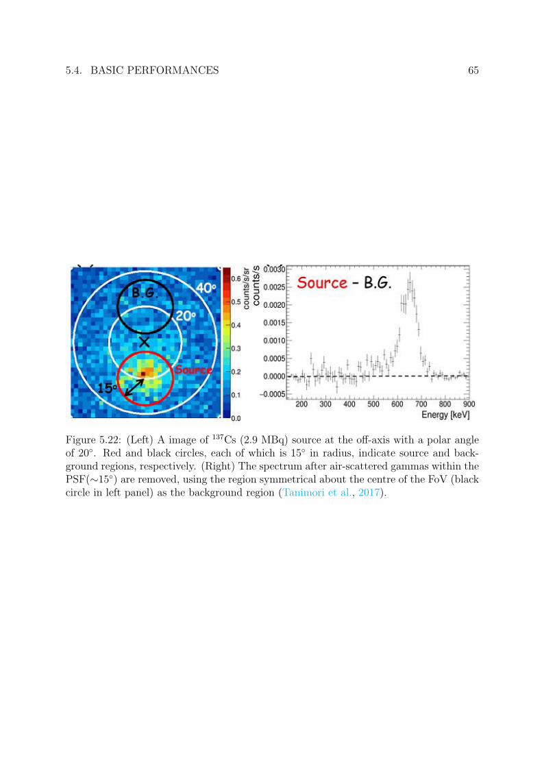
5.4. BASIC PERFORMANCES 65
Figure 5.22: (Left) A image of 137Cs (2.9 MBq) source at the off-axis with a polar angleof 20. Red and black circles, each of which is 15 in radius, indicate source and back-ground regions, respectively. (Right) The spectrum after air-scattered gammas within thePSF(∼15) are removed, using the region symmetrical about the centre of the FoV (blackcircle in left panel) as the background region (Tanimori et al., 2017).

Chapter 6
Simulation Studies of Polarization
Measurement
As discussed in Chapter 4, Compton cameras, including the ETCC, can be used as Imag-
ing Compton polarimeters. Compton camera determines the three-dimensional direction
of the scattered gamma-ray as the direction from the interaction point to the absorption
point and obtains the angular distribution of the scattered gamma-ray D(θdet, ϕdet) for
each gamma-ray. In addition, the ETCC uniquely determines the incident direction event
by event; therefore, θph and ϕph in the photon coordinate system can be geometrically
calculated. Therefore, the ETCC is able to estimate precisely the effect of an off-axis inci-
dence and hence enables us to measure the polarization within a large FoV. Furthermore,
due to powerful background suppressions with a sharp PSF and particle identification of
the electron tracks, we expect a much better MDP than that of standard Compton cam-
eras even in intense background conditions, such as space. To calculate the MDPs of the
ETCC, we estimated the modulation factor for various energetic gamma-rays, incident
directions, and polarization directions using Monte Carlo simulations.
6.1 Physics Model of the ETCC
We constructed a simulation software with a detailed geometrical model of the ETCC
(Sawano et al., 2014) based on the Geant4 tool kit (Agostinelli et al., 2003). To calculate
the detection efficiency, we used the Geant4 (ver. 4.9.5p01) and the Livermore package,
which supports the electromagnetic process of low-energy gamma rays with an energy
of less than 1 MeV. The detection efficiency were obtained mainly from the production
of two probabilities: that of Compton scattering and its recoil electron contained fully
in the TPC, and that of the full absorption of scattered gammas in the PSAs. The
electron drift and gas amplification in the gas volume, the uniformities of gain in TPC
and PSAs, and the data acquisition system were not included in the simulations. Despite
the simple constitution, the simulated detection efficiency well explains the detection
66
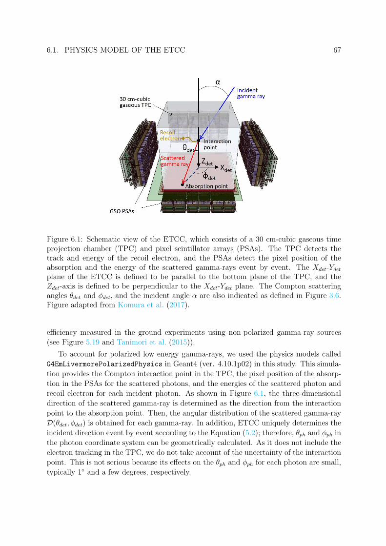
6.1. PHYSICS MODEL OF THE ETCC 67
Figure 6.1: Schematic view of the ETCC, which consists of a 30 cm-cubic gaseous timeprojection chamber (TPC) and pixel scintillator arrays (PSAs). The TPC detects thetrack and energy of the recoil electron, and the PSAs detect the pixel position of theabsorption and the energy of the scattered gamma-rays event by event. The Xdet-Ydet
plane of the ETCC is defined to be parallel to the bottom plane of the TPC, and theZdet-axis is defined to be perpendicular to the Xdet-Ydet plane. The Compton scatteringangles θdet and ϕdet, and the incident angle α are also indicated as defined in Figure 3.6.Figure adapted from Komura et al. (2017).
efficiency measured in the ground experiments using non-polarized gamma-ray sources
(see Figure 5.19 and Tanimori et al. (2015)).
To account for polarized low energy gamma-rays, we used the physics models called
G4EmLivermorePolarizedPhysics in Geant4 (ver. 4.10.1p02) in this study. This simula-
tion provides the Compton interaction point in the TPC, the pixel position of the absorp-
tion in the PSAs for the scattered photons, and the energies of the scattered photon and
recoil electron for each incident photon. As shown in Figure 6.1, the three-dimensional
direction of the scattered gamma-ray is determined as the direction from the interaction
point to the absorption point. Then, the angular distribution of the scattered gamma-ray
D(θdet, ϕdet) is obtained for each gamma-ray. In addition, ETCC uniquely determines the
incident direction event by event according to the Equation (5.2); therefore, θph and ϕph in
the photon coordinate system can be geometrically calculated. As it does not include the
electron tracking in the TPC, we do not take account of the uncertainty of the interaction
point. This is not serious because its effects on the θph and ϕph for each photon are small,
typically 1 and a few degrees, respectively.

68 6.2. EVENT RECONSTRUCTION
6.2 Event Reconstruction
Compton scattering events are selected according to the following criteria: (a) Compton
scattering occurs in the TPC volume, (b) the photoelectric absorption occurs in the PSA
for the scattering gamma-ray, (c) the recoil electron should be stopped in the TPC, (d)
the energy deposits in the TPC and PSA exceed the detector thresholds, and (e) without
the loss of the incident photon energy within a certain energy resolution. Here the particle
identification by dE/dx of a recoil electron is emulated by the criteria ‘c’. For the real
detector, the detector thresholds are set to be 1 keV and 90 keV for TPC and PSA,
respectively. We used the energy resolutions of the TPC and PSA following Gaussian
distribution with the FWHM of 22% for 22 keV and 11% for 662 keV, respectively, having
an energy dependence of E−0.5 due to statistical fluctuations from the measurement of the
instrument.
On-axis incidence case
After applying the event selection criteria, the angular distribution of scattered gamma-
rays D(cos θdet, ϕdet) and the integrated azimuthal angle distribution N (ϕdet) are ob-
tained as shown in Figure 6.2 for 200-keV incident gamma-rays, with an incident angle
α set to zero (on-axis incidence) and a polarization direction along the Xdet-axis. Fig-
ure 6.2(a) shows Dnon(cos θdet, ϕdet) for non-polarized incident gamma-rays, and Figure
6.2(b) shows Dpol(cos θdet, ϕdet) for 100% linearly polarized incident gamma-rays. In both
figures, Compton-scattered photons absorbed in the bottom PSAs are modulated near
cos θdet = 1 (i.e., forward scattering events). In Figure 6.2(a), events absorbed in the
four side PSAs are modulated near values of ϕdet of −180, −90, 0, 90, and 180 in
the range of cos θdet between −1.0 and 0.8. Conversely, in Figure 6.2(b), many events
are modulated near values of ϕdet of −90 and 90, where the direction of the incident
gamma-ray is perpendicular to the polarization direction of the incident photon and the
Compton scattering cross section is at its maximum according to Equation (3.3). The
azimuthal distributions N (ϕdet)s integrated over θdet are calculated according to
N (ϕdet) =
∫ (cos θ)max
−1
D(cos θdet, ϕdet)d(cos θdet) (6.1)
which is derived from Equation (3.8). Figures 6.2(c) and 6.2(d) show Nnon(ϕdet) and
Npol(ϕdet), respectively. We found that, in Nnon(ϕdet), a small systematic modulation
appears due to the non-uniformity of the detector response, as mentioned in Section 3.2.2.
Figure 6.3 shows the azimuthal angle distribution Ncor(ϕdet) corrected for the response
effect according to Equation (3.21) with the best fit curve given by Equation (3.13); the
modulation factor of the ETCC is estimated to be 0.52 ± 0.01 for on-axis incident photons
with energies of 200 keV.
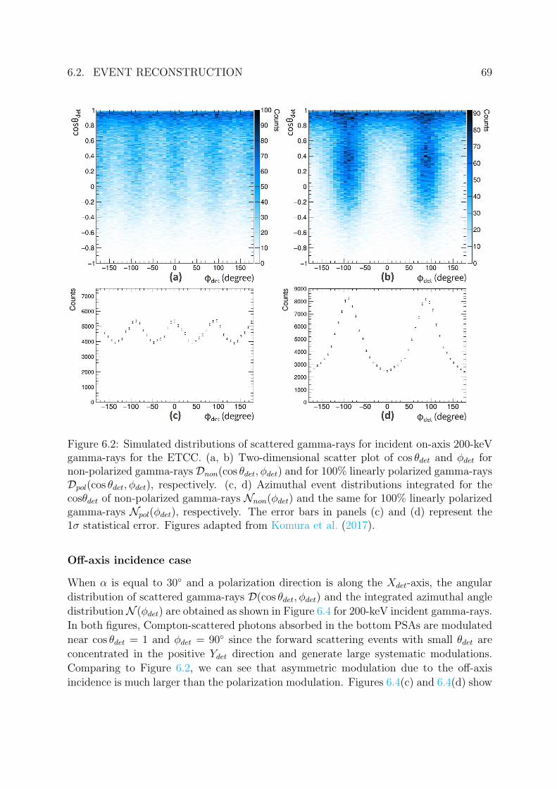
6.2. EVENT RECONSTRUCTION 69
Figure 6.2: Simulated distributions of scattered gamma-rays for incident on-axis 200-keVgamma-rays for the ETCC. (a, b) Two-dimensional scatter plot of cos θdet and ϕdet fornon-polarized gamma-rays Dnon(cos θdet, ϕdet) and for 100% linearly polarized gamma-raysDpol(cos θdet, ϕdet), respectively. (c, d) Azimuthal event distributions integrated for thecosθdet of non-polarized gamma-rays Nnon(ϕdet) and the same for 100% linearly polarizedgamma-rays Npol(ϕdet), respectively. The error bars in panels (c) and (d) represent the1σ statistical error. Figures adapted from Komura et al. (2017).
Off-axis incidence case
When α is equal to 30 and a polarization direction is along the Xdet-axis, the angular
distribution of scattered gamma-rays D(cos θdet, ϕdet) and the integrated azimuthal angle
distributionN (ϕdet) are obtained as shown in Figure 6.4 for 200-keV incident gamma-rays.
In both figures, Compton-scattered photons absorbed in the bottom PSAs are modulated
near cos θdet = 1 and ϕdet = 90 since the forward scattering events with small θdet are
concentrated in the positive Ydet direction and generate large systematic modulations.
Comparing to Figure 6.2, we can see that asymmetric modulation due to the off-axis
incidence is much larger than the polarization modulation. Figures 6.4(c) and 6.4(d) show

70 6.2. EVENT RECONSTRUCTION
Figure 6.3: Corrected integrated azimuthal angle distribution of scattered photonNcor(ϕdet) calculated from Npol(ϕdet)/Nnon(ϕdet). Figure adapted from Komura et al.(2017).
Nnon(ϕdet) and Npol(ϕdet), respectively. If we applied the cancellation of the effect due to
the non-uniformity of the detector response to Npol(ϕdet) according to Equation (4), the
obtained azimuthal angle distribution Ncor(ϕdet) is far from a symmetrical distribution,
as shown in Figure 6.5. From this response-corrected azimuthal angle distribution, we
obtained a modulation factor of 0.45 ± 0.01, which is not reliable.
As mentioned in Section 3.2.3, we first have to transform the coordinate system to
the photon system and calculate the azimuthal angle distribution in this system before
canceling out the non-uniform response. Figure 6.6 shows the angular distribution of scat-
tered gamma-rays D(cos θph, ϕph) and the integrated azimuthal angle distribution N (ϕph)
in photon coordinate system calculated from D(cos θdet, ϕdet) according to Equation (3.24)
assuming (α, β) = (30, 0). Figure 6.7 shows the azimuthal angle distribution Ncor(ϕph)
with the best fit curve given by Equation (3.13), where the symmetries are obviously
recovered. The modulation factor of the ETCC is estimated to be 0.53 ± 0.01 for on-axis
incident photons with energies of 200 keV. Thanks to the transformation of the coordinate
system to the photon system, the modulation factor is nearly independent of the incident
gamma-ray direction.

6.2. EVENT RECONSTRUCTION 71
Figure 6.4: Simulated distributions of scattered gamma-rays for incident 200-keV gamma-rays for the ETCC, when the incident angle is equal to 30. (a, b) Two-dimensionalscatter plot of cos θph and ϕph for non-polarized gamma-rays Dnon(cos θdet, ϕdet) and for100% linearly polarized gamma-rays Dpol(cos θdet, ϕdet), respectively. (c, d) Azimuthalevent distributions integrated for the cosθdet of non-polarized gamma-rays Nnon(ϕdet) andthe same for 100% linearly polarized gamma-rays Npol(ϕdet), respectively. The error barsin panels (c) and (d) represent the 1σ statistical error.

72 6.2. EVENT RECONSTRUCTION
Figure 6.5: Corrected integrated azimuthal angle distribution of scattered photonNcor(ϕdet) calculated from Npol(ϕdet)/Nnon(ϕdet).
Figure 6.6: Same plots as shown in Figure 6.4 in the photon coordinate system.
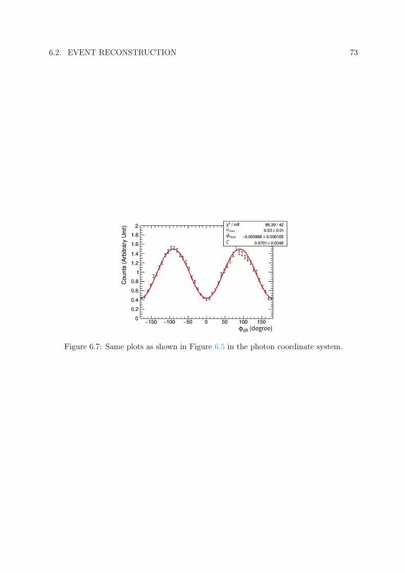
6.2. EVENT RECONSTRUCTION 73
Figure 6.7: Same plots as shown in Figure 6.5 in the photon coordinate system.
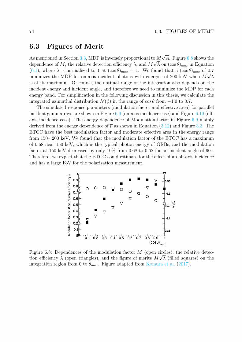
74 6.3. FIGURES OF MERIT
6.3 Figures of Merit
As mentioned in Section 3.3, MDP is inversely proportional toM√A. Figure 6.8 shows the
dependence of M , the relative detection efficiency λ, and M√λ on (cos θ)max in Equation
(6.1), where λ is normalized to 1 at (cos θ)max = 1. We found that a (cos θ)max of 0.7
minimizes the MDP for on-axis incident photons with energies of 200 keV when M√λ
is at its maximum. Of course, the optimal range of the integration also depends on the
incident energy and incident angle, and therefore we need to minimize the MDP for each
energy band. For simplification in the following discussion in this thesis, we calculate the
integrated azimuthal distribution N (ϕ) in the range of cos θ from −1.0 to 0.7.
The simulated response parameters (modulation factor and effective area) for parallel
incident gamma-rays are shown in Figure 6.9 (on-axis incidence case) and Figure 6.10 (off-
axis incidence case). The energy dependence of Modulation factor in Figure 6.9 mainly
derived from the energy dependence of µ as shown in Equation (3.12) and Figure 3.3. The
ETCC have the best modulation factor and moderate effective area in the energy range
from 150– 200 keV. We found that the modulation factor of the ETCC has a maximum
of 0.68 near 150 keV, which is the typical photon energy of GRBs, and the modulation
factor at 150 keV decreased by only 10% from 0.68 to 0.62 for an incident angle of 90.
Therefore, we expect that the ETCC could estimate for the effect of an off-axis incidence
and has a large FoV for the polarization measurement.
Figure 6.8: Dependences of the modulation factor M (open circles), the relative detec-tion efficiency λ (open triangles), and the figure of merits M
√λ (filled squares) on the
integration region from 0 to θmax. Figure adapted from Komura et al. (2017).
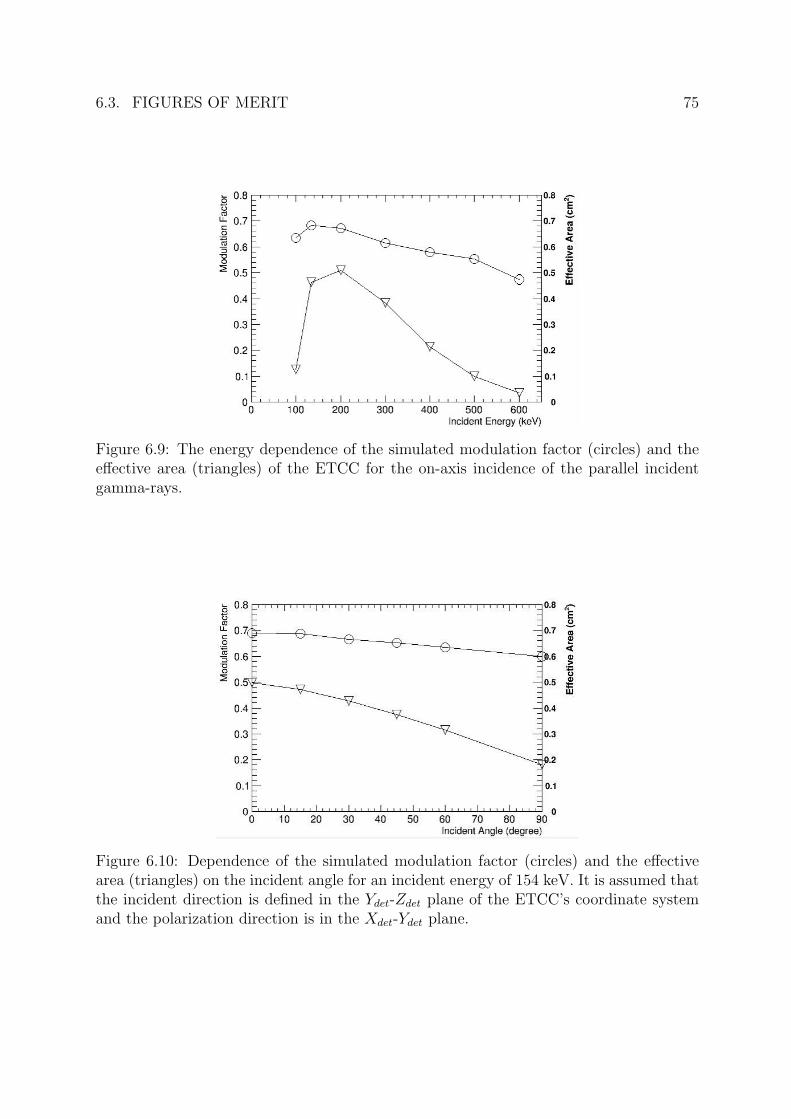
6.3. FIGURES OF MERIT 75
Figure 6.9: The energy dependence of the simulated modulation factor (circles) and theeffective area (triangles) of the ETCC for the on-axis incidence of the parallel incidentgamma-rays.
Figure 6.10: Dependence of the simulated modulation factor (circles) and the effectivearea (triangles) on the incident angle for an incident energy of 154 keV. It is assumed thatthe incident direction is defined in the Ydet-Zdet plane of the ETCC’s coordinate systemand the polarization direction is in the Xdet-Ydet plane.

Chapter 7
Experiment on a Polarized X-ray
Beam
We performed two types of experiments from January 27–31, 2015, using the ETCC on the
High Energy Inelastic Scattering Beamline BL08W at SPring-8, which supplies a > 99%
linearly polarized hard X-ray beam with an energy of 182 keV.
7.1 Setup of the ETCC
Figure 7.1 is the photograph of the experimental setup. The intensity of the X-ray beam
was considerably weakened by 20 cm thick Al attenuators to avoid damage in the ETCC,
and to set an acceptable photon rate for the ETCC’s electronics. The X-ray beam passed
through at 13 cm above the ETCC. The polarization direction of the beam is always
horizontal. The front and back sides of the ETCC in the beam direction were shielded
by 1mm thick lead sheets to reduce chance coincidence event between the TPC and the
PSAs due to ambient X-rays in the laboratory. However, the side faces of the ETCC were
not covered because of the lack of lead sheets; a large amount of chance coincidence event
occurred as described below.
7.2 On-axis Incident Case
In the first experiment, we measured the modulation factor of the ETCC and compared it
with our simulation results for an on-axis beam with various polarization directions. The
experimental setup is shown in Figure 7.2(a). We irradiated the X-ray beam to a 10-mm
thick aluminum (Al) target, from which X-rays scattered vertically at the target entered
the ETCC. The (Xdet, Ydet) coordinates of the beam spot on the Al target were set to (10
mm, 0 mm). Due to spatial limitations in the laboratory, the Al target was located at
a height of 13 cm just above the ETCC. Scattered X-rays at the Al target were roughly
collimated with an opening window (10 cm × 10 cm) in the lead blocks set at the top of
76

7.2. ON-AXIS INCIDENT CASE 77
Figure 7.1: Photograph of the ETCC installed for the beam experiment at SPring-8BL08W.
the TPC as shown in Figure 7.3, and therefore the energy and the degree of polarization
of the incident X-rays were widely spread from 123 to 148 keV and from 93% to 98%,
respectively. As shown in Figure 7.2(b), the ETCC measured the angular distribution of
the Compton scattered X-rays for five different incident X-ray polarization directions by
rotating the ETCC around its Zdet-axis. First, the azimuthal angle of the polarization
direction of the X-ray beam was set to 0. The event rate with the Al target (on-target
measurement) was approximately 300 Hz and contained huge background levels due to
air scattering, approximately three times larger than that expected at balloon altitude
(Mizumoto et al., 2015). We performed the measurement with no Al target (off-target
measurement) for each polarization direction to subtract backgrounds from the on-target
data in the off-line analysis.
To obtain correctly reconstructed Compton events, we performed the same event se-
lections mentioned in Section 5.3. First, we selected the correct Compton event, where
the recoil electron stops in the TPC, using the relationship between the measured track

78 7.2. ON-AXIS INCIDENT CASE
Figure 7.2: (a) A side view in the Ydet-Zdet plane of the ETCC setup for the first ex-periments on BL08W at SPring-8. The origin of the coordinate system of the ETCC(XdetYdetZdet) was set at the bottom center of the TPC. (b) The ETCC measured theangular distribution D(θdet, ϕdet) of the scattered X-ray in the TPC, where θdet and ϕdet
are the polar scattering angle and the azimuthal scattering angle, respectively. The mea-surements were performed for five different polarization directions of the X-ray beam byrotating the ETCC in the Xdet-Ydet plane. The corresponding azimuthal angles are 0,−22.5, −45, −90, and −180. Figures adapted from Komura et al. (2017).
range and the energy deposited in the TPC as described below:(Track Range
[mm]
)< 4.1× 10³
(Energy Deposit
[MeV]
)1.8
+ 50, (7.1)
which is drawn as the solid line in Figure 7.4(a). Next, we selected the events interacting
in the fiducial volume of the TPC. Figure 7.4(b) shows the distribution of the analyzed
starting positions of the measured tracks (i.e., the Compton scattering positions) along
the Zdet-axis. The coincidence events between TPC and PSAs lay within the region of
approximately −340 mm < Zdet < 0 mm, which includes both the signal X-rays scattered
on the inside of the TPC and the chance coincidence background due to air scattering. The
remaining areas are all formed by the chance coincidence background, in which the time lag
between incidents on TPC and PSAs is longer than the time window of the coincidence.
We defined the fiducial gas volume region as −319.9 mm < Zdet < -7.9 mm, and we
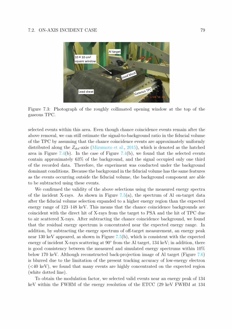
7.2. ON-AXIS INCIDENT CASE 79
Figure 7.3: Photograph of the roughly collimated opening window at the top of thegaseous TPC.
selected events within this area. Even though chance coincidence events remain after the
above removal, we can still estimate the signal-to-background ratio in the fiducial volume
of the TPC by assuming that the chance coincidence events are approximately uniformly
distributed along the Zdet-axis (Mizumoto et al., 2015), which is denoted as the hatched
area in Figure 7.4(b). In the case of Figure 7.4(b), we found that the selected events
contain approximately 63% of the background, and the signal occupied only one third
of the recorded data. Therefore, the experiment was conducted under the background
dominant conditions. Because the background in the fiducial volume has the same features
as the events occurring outside the fiducial volume, the background component are able
to be subtracted using these events.
We confirmed the validity of the above selections using the measured energy spectra
of the incident X-rays. As shown in Figure 7.5(a), the spectrum of Al on-target data
after the fiducial volume selection expanded to a higher energy region than the expected
energy range of 123–148 keV. This means that the chance coincidence backgrounds are
coincident with the direct hit of X-rays from the target to PSA and the hit of TPC due
to air scattered X-rays. After subtracting the chance coincidence background, we found
that the residual energy spectrum is concentrated near the expected energy range. In
addition, by subtracting the energy spectrum of off-target measurement, an energy peak
near 130 keV appeared, as shown in Figure 7.5(b), which is consistent with the expected
energy of incident X-rays scattering at 90 from the Al target, 134 keV; in addition, there
is good consistency between the measured and simulated energy spectrums within 10%
below 170 keV. Although reconstructed back-projection image of Al target (Figure 7.6)
is blurred due to the limitation of the present tracking accuracy of low-energy electron
(<40 keV), we found that many events are highly concentrated on the expected region
(white dotted line).
To obtain the modulation factor, we selected valid events near an energy peak of 134
keV within the FWHM of the energy resolution of the ETCC (29 keV FWHM at 134
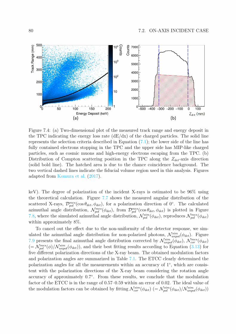
80 7.2. ON-AXIS INCIDENT CASE
Figure 7.4: (a) Two-dimensional plot of the measured track range and energy deposit inthe TPC indicating the energy loss rate (dE/dx) of the charged particles. The solid linerepresents the selection criteria described in Equation (7.1); the lower side of the line hasfully contained electrons stopping in the TPC and the upper side has MIP-like chargedparticles, such as cosmic muons and high-energy electrons escaping from the TPC. (b)Distribution of Compton scattering position in the TPC along the Zdet-axis direction(solid bold line). The hatched area is due to the chance coincidence background. Thetwo vertical dashed lines indicate the fiducial volume region used in this analysis. Figuresadapted from Komura et al. (2017).
keV). The degree of polarization of the incident X-rays is estimated to be 96% using
the theoretical calculation. Figure 7.7 shows the measured angular distribution of the
scattered X-rays, Dmespol (cos θdet, ϕdet), for a polarization direction of 0. The calculated
azimuthal angle distribution, Nmespol (ϕdet), from Dmes
pol (cos θdet, ϕdet) is plotted in Figure
7.8, where the simulated azimuthal angle distribution, N simpol (ϕdet), reproduces Nmes
pol (ϕdet)
within approximately 8%.
To cancel out the effect due to the non-uniformity of the detector response, we sim-
ulated the azimuthal angle distribution for non-polarized photons, N simunpol(ϕdet). Figure
7.9 presents the final azimuthal angle distribution corrected by N simunpol(ϕdet), Nmes
cor (ϕdet)
(= Nmespol (ϕ)/N sim
unpol(ϕdet)), and their best fitting results according to Equation (3.13) for
five different polarization directions of the X-ray beam. The obtained modulation factors
and polarization angles are summarized in Table 7.1. The ETCC clearly determined the
polarization angles for all the measurements within an accuracy of 1, which are consis-
tent with the polarization directions of the X-ray beam considering the rotation angle
accuracy of approximately 0.7. From these results, we conclude that the modulation
factor of the ETCC is in the range of 0.57–0.59 within an error of 0.02. The ideal value of
the modulation factors can be obtained by fitting N simcor (ϕdet) (= N sim
pol (ϕdet)/N simunpol(ϕdet))

7.2. ON-AXIS INCIDENT CASE 81
Figure 7.5: (a) Subtraction of the chance coincidence background from the measuredenergy spectrum of the incident X-rays. The energy spectrum of the Al on-target dataafter the fiducial volume selection (red), the chance coincidence background (blue), andthe residual events (green) after the subtraction of the chance coincidence backgroundare shown. The blue line is obtained by sampling and scaling the energy distributionof the events lying between Zdet < −340 mm and Zdet > 0 mm. (b) Subtraction ofthe Al off-target data and the final reconstructed energy spectrum. The red and bluelines represent the Al on-target and off-target data, respectively, after the removal of thechance coincidence background. The green line represents the residual events after thesubtraction of the off-target data, which is in good agreement with the simulated spectrum(filled triangles). The error bars in panels (a) and (b) represent the 1σ statistical error(Komura et al., 2017).
and are also included in Table 7.1. The differences between the measured and simulated
modulation factors are larger than the margin of errors due to the small differences in
the azimuthal angle distributions and because the uncertainty in the simulation does not
take into account the position resolution of the Compton interaction point in the TPC.

82 7.2. ON-AXIS INCIDENT CASE
Figure 7.6: Reconstructed back-projection image of Al target.
Figure 7.7: Two-dimensional scatter plot of the measured Dmespol (cos θdet, ϕdet) when the
polarization direction of the X-ray beam is 0. Figure adapted from Komura et al. (2017).

7.2. ON-AXIS INCIDENT CASE 83
Figure 7.8: The solid line histogram represents the measured azimuthal angle distributionNmes
pol (ϕdet). The simulation results of the azimuthal angle distribution N simpol (ϕdet) and
N simunpol(ϕdet) are plotted as filled circles and open circles, respectively. Figure adapted
from Komura et al. (2017).

84 7.2. ON-AXIS INCIDENT CASE
Figure 7.9: Corrected modulation curves (open squares) and the best fit curves (solidlines). The polarization direction of the X-ray beam is 0, −22.5, −45, −90, and−180, respectively, from top to bottom. Figure adapted from Komura et al. (2017).
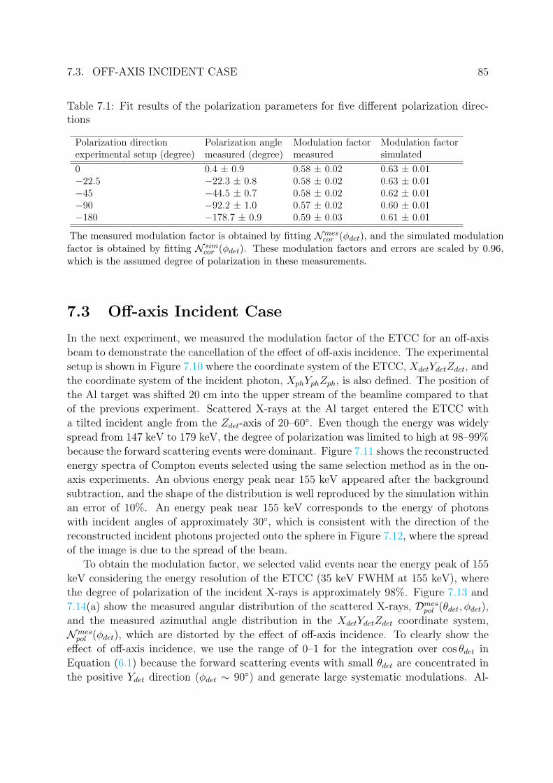
7.3. OFF-AXIS INCIDENT CASE 85
Table 7.1: Fit results of the polarization parameters for five different polarization direc-tions
Polarization direction Polarization angle Modulation factor Modulation factorexperimental setup (degree) measured (degree) measured simulated
0 0.4 ± 0.9 0.58 ± 0.02 0.63 ± 0.01−22.5 −22.3 ± 0.8 0.58 ± 0.02 0.63 ± 0.01−45 −44.5 ± 0.7 0.58 ± 0.02 0.62 ± 0.01−90 −92.2 ± 1.0 0.57 ± 0.02 0.60 ± 0.01−180 −178.7 ± 0.9 0.59 ± 0.03 0.61 ± 0.01
The measured modulation factor is obtained by fitting Nmescor (ϕdet), and the simulated modulation
factor is obtained by fitting N simcor (ϕdet). These modulation factors and errors are scaled by 0.96,
which is the assumed degree of polarization in these measurements.
7.3 Off-axis Incident Case
In the next experiment, we measured the modulation factor of the ETCC for an off-axis
beam to demonstrate the cancellation of the effect of off-axis incidence. The experimental
setup is shown in Figure 7.10 where the coordinate system of the ETCC, XdetYdetZdet, and
the coordinate system of the incident photon, XphYphZph, is also defined. The position of
the Al target was shifted 20 cm into the upper stream of the beamline compared to that
of the previous experiment. Scattered X-rays at the Al target entered the ETCC with
a tilted incident angle from the Zdet-axis of 20–60. Even though the energy was widely
spread from 147 keV to 179 keV, the degree of polarization was limited to high at 98–99%
because the forward scattering events were dominant. Figure 7.11 shows the reconstructed
energy spectra of Compton events selected using the same selection method as in the on-
axis experiments. An obvious energy peak near 155 keV appeared after the background
subtraction, and the shape of the distribution is well reproduced by the simulation within
an error of 10%. An energy peak near 155 keV corresponds to the energy of photons
with incident angles of approximately 30, which is consistent with the direction of the
reconstructed incident photons projected onto the sphere in Figure 7.12, where the spread
of the image is due to the spread of the beam.
To obtain the modulation factor, we selected valid events near the energy peak of 155
keV considering the energy resolution of the ETCC (35 keV FWHM at 155 keV), where
the degree of polarization of the incident X-rays is approximately 98%. Figure 7.13 and
7.14(a) show the measured angular distribution of the scattered X-rays, Dmespol (θdet, ϕdet),
and the measured azimuthal angle distribution in the XdetYdetZdet coordinate system,
Nmespol (ϕdet), which are distorted by the effect of off-axis incidence. To clearly show the
effect of off-axis incidence, we use the range of 0–1 for the integration over cos θdet in
Equation (6.1) because the forward scattering events with small θdet are concentrated in
the positive Ydet direction (ϕdet ∼ 90) and generate large systematic modulations. Al-

86 7.3. OFF-AXIS INCIDENT CASE
Figure 7.10: A side view in the Ydet–Zdet plane of the ETCC setup for the second experi-ment on BL08W at SPring-8. The Al target was shifted 20 cm into the upper stream ofthe beamline than in the previous experiment. The photon coordinate system XphYphZph
has the Zph-axis along the average direction of the incident photons, and the Xph-axiscoincides with the Xdet–Ydet plane. Figure adapted from Komura et al. (2017).
Figure 7.11: Reconstructed energy spectra of the incident photons. The red and blue linesrepresent the spectra for the Al on-target and off-target data, respectively. The green lineis the difference between the red and blue lines, which corresponds to the pure energyspectrum of the incident X-rays after subtracting the background due to air scattering.There is good consistency between the green line and the simulated results (the filledtriangles) near the energy peak at 154 keV (Komura et al., 2017).
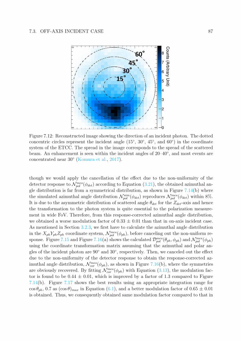
7.3. OFF-AXIS INCIDENT CASE 87
Figure 7.12: Reconstructed image showing the direction of an incident photon. The dottedconcentric circles represent the incident angle (15, 30, 45, and 60) in the coordinatesystem of the ETCC. The spread in the image corresponds to the spread of the scatteredbeam. An enhancement is seen within the incident angles of 20–40, and most events areconcentrated near 30 (Komura et al., 2017).
though we would apply the cancellation of the effect due to the non-uniformity of the
detector response to Nmespol (ϕdet) according to Equation (3.21), the obtained azimuthal an-
gle distribution is far from a symmetrical distribution, as shown in Figure 7.14(b) where
the simulated azimuthal angle distribution N simpol (ϕdet) reproduces Nmes
pol (ϕdet) within 8%.
It is due to the asymmetric distribution of scattered angle θdet for the Zdet-axis and hence
the transformation to the photon system is quite essential to the polarization measure-
ment in wide FoV. Therefore, from this response-corrected azimuthal angle distribution,
we obtained a worse modulation factor of 0.33 ± 0.01 than that in on-axis incident case.
As mentioned in Section 3.2.3, we first have to calculate the azimuthal angle distribution
in the XphYphZph coordinate system, Nmespol (ϕph), before canceling out the non-uniform re-
sponse. Figure 7.15 and Figure 7.16(a) shows the calculated Dmespol (θph, ϕph) and Nmes
pol (ϕph)
using the coordinate transformation matrix assuming that the azimuthal and polar an-
gles of the incident photon are 90 and 30, respectively. Then, we canceled out the effect
due to the non-uniformity of the detector response to obtain the response-corrected az-
imuthal angle distribution, Nmescor (ϕph), as shown in Figure 7.16(b), where the symmetries
are obviously recovered. By fitting Nmescor (ϕph) with Equation (3.13), the modulation fac-
tor is found to be 0.44 ± 0.01, which is improved by a factor of 1.3 compared to Figure
7.14(b). Figure 7.17 shows the best results using an appropriate integration range for
cos θph, 0.7 as (cos θ)max in Equation (6.1), and a better modulation factor of 0.65 ± 0.01
is obtained. Thus, we consequently obtained same modulation factor compared to that in
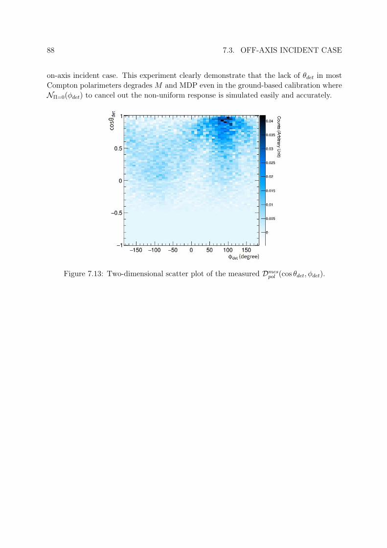
88 7.3. OFF-AXIS INCIDENT CASE
on-axis incident case. This experiment clearly demonstrate that the lack of θdet in most
Compton polarimeters degrades M and MDP even in the ground-based calibration where
NΠ=0(ϕdet) to cancel out the non-uniform response is simulated easily and accurately.
Figure 7.13: Two-dimensional scatter plot of the measured Dmespol (cos θdet, ϕdet).

7.3. OFF-AXIS INCIDENT CASE 89
Figure 7.14: (a) Azimuthal angle distributions in the XdetYdetZdet coordinate sys-tem: Nmes
pol (ϕdet) (solid line histogram), N simpol (ϕdet) (filled circles) and N sim
unpol(ϕdet)(open circles). (b) Corrected azimuthal angle distribution (open squares) calculatedby Nmes
pol (ϕdet)/N simunpol(ϕdet) and the best fitted curve (solid line). Figures adapted from
Komura et al. (2017).

90 7.3. OFF-AXIS INCIDENT CASE
Figure 7.15: Two-dimensional scatter plot of the Dmespol (cos θph, ϕph) in the XphYphZph
coordinate system.
Figure 7.16: Same plots as shown in Figure 7.14 in the XphYphZph coordinate system.Figures adapted from Komura et al. (2017).
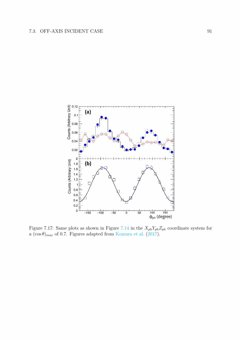
7.3. OFF-AXIS INCIDENT CASE 91
Figure 7.17: Same plots as shown in Figure 7.14 in the XphYphZph coordinate system fora (cos θ)max of 0.7. Figures adapted from Komura et al. (2017).

Chapter 8
Discussion and Conclusion
We present a novel approach for a gamma-ray imaging spectroscopic polarimeter for all-
sky surveys using an ETCC, which provides highly-sensitive polarimetry and imaging
spectroscopy based on optics for each object, including both persistent and transient
objects within its wide FoV of up to 2π sr all at once. The ETCC provides robust
solutions to two major difficulties with wide FoV polarimetry, i.e., huge backgrounds
coming from all directions and the degradation of the modulation factor due to the effect
of off-axis incidence. It has already been demonstrated that an ETCC efficiently reject
both photon and non-photon backgrounds even in intense radiation conditions similar
to space using its excellent imaging performance based on a well-defined PSF and its
particle identification using dE/dx (Tanimori et al., 2015). Furthermore, the ETCC is
expected to maintain its modulation factor without degradation over its wide FoV because
it measures all the required information to analytically correct for the effect of off-axis
incidence, such as the three-dimensional direction of the scattered photons and the arrival
direction and energy of incident photons for each event. To examine these capabilities, we
performed a beam test of the current ETCC using a linearly polarized hard X-ray beam
at SPring-8. Although there were huge backgrounds of more than twice the polarized X-
ray signal, after background rejection, we obtained a modulation factor of 0.58 ± 0.02 at
134 keV for the quasi-on-axis incidence, which includes the deteriorating factor of oblique
incident angles of at most 21. As the greatest impact of this work, we demonstrated for
the first time a precise polarization measurement for off-axis incidence with an incident
angle of 30 on average; we confirmed that the ETCC can correct the distortion of the
measured polarization modulation due to off-axis incidence using the measured gamma-
ray image, and the obtained modulation factor was 0.65 ± 0.01 at 154 keV, which is
not degraded compared to that of quasi-on-axis incidence. According to the simulated
modulation factors for parallel incident gamma-rays as shown in Figure 8.1, we found that
the modulation factor of the ETCC has a maximum of 0.68 near 150 keV, which is the
typical photon energy of GRBs, and the modulation factor at 150 keV decreased by only
10% from 0.68 to 0.62 for an incident angle of 90. These simulated modulation factors
92
93
are consistent with the experimental ones even though they are affected by non-parallel
incidence and large backgrounds. Therefore, we conclude that the ETCC has a promising
potential to perform the wide FoV polarimetry maintaining its high modulation factor of
over 0.6 near 150 keV, at least for incident angles less than 30.
We plan to carry on an all-sky imaging survey using the ETCCs, which are improved
from the present ETCCs, in long-duration balloons and satellite experiments with 10 times
and 100 times, respectively, better sensitivity than that of COMPTEL (Tanimori et al.,
2015). In addition, these ETCCs will simultaneously provide polarization measurements
of bright objects. First, we will calculate the MDPs in the energy range of 100–300 keV for
the balloon observations. For long-duration balloon experiment, we designed an ETCC
consisting of 30-cm-cubic ETCC whose effective area would reach 11 cm2 at 200 keV
(Tanimori et al., 2015) and PSF would be 23 at the incident energy of 200 keV and a few
degrees over the incident energy of 600 keV (Tanimori et al., 2017). The background rate
at balloon altitude is estimated to be approximately 0.11 ph cm−2 s−1, which includes
extragalactic diffuse gamma-rays, atmospheric gamma-rays, and intrinsic gamma-rays
calculated by the Geant4 simulations based on results of previous balloon experiments
using a small ETCC (Takada et al., 2011). The MDPs at 99% confidence level for the
Crab nebula and Cygnus X-1 are calculated as approximately 20% and 30%, respectively,
according to Equation (3.26) in one-day balloon flights with 10 hours of observation.
Therefore, the ETCC could confirm the observations of INTEGRAL, which reported
that the degree of polarization of the Crab nebula is approximately 40% (Dean et al.,
2008; Forot et al., 2008). Thanks to the large FoV of the ETCC, we expect to survey
transient objects, in particular typical GRBs with moderate brightness. Note that, in
observations of transients using ETCC, we do not always need simultaneous observations
by other satellites to know the energy and direction of the targets, therefore ETCC can
perform polarization measurements of all the GRBs in its FoV. In long-duration balloon
experiments, we will use four ETCCs whose effective area would reach 44 cm2 (4×11
cm2) at an incident energy of 200 keV. The MDP of an ETCC for GRBs with an intensity
10−5 erg cm−2 is calculated to be approximately 25%. Even if such GRBs had a long
duration of several tens of seconds, it is expected that the MDP will degrade less than
5% thanks to the powerful ETCC background suppression. If we assume that the degree
of polarization of the GRBs is greater than 30%, we expect to observe approximately
2–3 GRBs during a one-month balloon-flight; this is estimated from the fluence and the
duration parameter T90 of GRB samples based on the BATSE Current Gamma-Ray Burst
Catalog. Next, we will calculate the MDPs in the energy range of 100–300 keV for the
satellite observations. For a middle-class satellite experiment, we designed an ETCC
consisting of four 50-cm-cubic ETCCs whose effective area would reach 280 cm2 (4×70
cm2) at 200 keV (Tanimori et al., 2015). Using the effective area of the satellite-ETCC, we
calculated the MDPs with respect to the source flux as shown in Figure 8.2. We estimate
that the MDPs at 13 mCrab would be approximately 10% for an observation time of 107
s. Utilizing advantage of wide-FoV, the satellite-ETCC will contribute to the exploration
94
of polarized serendipity sources as well as major gamma-ray objects, such as AGNs,
BBHs, and pulsars at the same level of MDP as that of the pointing X-ray polarimeters.
Simultaneously, we expect that the satellite-ETCC will measure over 20 GRBs that have
a fluence of more than 6 × 10⁻⁶ erg cm−2 and polarization degree of more than 10%
during a one-year observation. The number of expected GRBs per year is comparable
to that of the largest-scale missions, such as POLAR (Orsi & Polar Collaboration, 2011);
therefore, the satellite-ETCC will contribute to the desired statistical observations of GRB
polarizations.
As discussed in Chapter 3, to achieve the MDP at the same level as that of the point-
ing X-ray polarimeters, the wide-FoV gamma-ray polarimeter should have the following
characteristics: (1) high M and large effective area to suppress the statistical fluctuation
of signal photon; (2) imaging ability based on a well-defined PSF to verify the reliability
of the correction of non-uniform response and to subtract the background components of
N (ϕdet); (3) measuring θdet and source direction to cancel out the effect of off-axis inci-
dence; (4) background rejection power to reduce the background contribution to N (ϕdet),
especially the imaging ability based on a sharp PSF is essential. Although several pro-
posed GRB polarimeters have moderate M ∼ 0.5 and effective area ∼ 100 cm2, they do
not have the capability of imaging and measuring θdet: MDP is largely degraded due to
the lack of requirements (2), (3), and (4). Conventional Compton cameras measure both
ϕdet and θdet event by event, therefore they have the potential to measure the polarization
without the degradation of MDP due to the effect of off-axis incidence. However the
source direction is determined as the circle direction, which is not sufficient to defined the
PSF and to satisfy requirements (2) and (4). Although Compton camera is effective to
observe the very bright GRBs, the MDP become too high to measure the polarization of
low signal-to-noise gamma-ray objects. To lower the MDP enough to observe the faint
GRBs and persistent objects, the imaging ability based on a well-defined and sharp PSF is
essential. Consequently, we conclude that the imaging polarimetry using an ETCC, which
has the potential to provide a well-defined and sharp PSF and satisfy all the requirements
(1)–(4), is the only approach to perform the all-sky gamma-ray polarization survey for
both transient and persistent objects of ∼10 mCrab with 10% polarization level.

95
Figure 8.1: (a) The energy dependence of the simulated modulation factor (circles) ofthe current ETCC for the on-axis incidence of the parallel incident gamma-rays. Themeasured (filled squares) and simulated (open squares) modulation factors obtained inSection 7.2 are also plotted. The modulation factors of the experiment are 9%–15%smaller than that of the simulated one at 134 keV due to the non-parallel incidence andthe residual backgrounds in the experiment. (b) Dependence of the simulated modulationfactor (circles) on the incident angle for an incident energy of 154 keV. It is assumedthat the incident direction is defined in the Y -Z plane of the ETCC’s coordinate systemand the polarization direction is in the X-Y plane. The modulation factors obtained inSection 7.2 are plotted at an incident angle of 0 using the same symbols as in panel(a). The measured (filled triangles) and simulated (open triangles) modulation factorsobtained in Section 7.3 are also plotted at an incident angle of 30 (Komura et al., 2017).

96
Figure 8.2: Solid line showing the calculated MDPs of the satellite-ETCC as a functionof the source flux in the energy range of 100–300 keV for an observation time of 107 s.The dashed vertical lines represent source fluxes of 1, 1/10, and 1/100 the Crab nebula(Komura et al., 2017).

Acknowledgments
I am deeply grateful to Prof. Toru Tanimori for his guidance and encouragements in this
work. I would also like to my gratitude to Dr. Atsuhi Takada for a plenty of insightful
comments. I specially thanks the µ-PIC collaborators: Associate Prof. Hidetoshi Kubo,
Dr. Yositaka Mizumura, Dr. Tetsuya Mizumoto, Dr. Shinya Sonoda, Dr. Dai Tomono,
Dr. Shunsuke Kurosawa, Dr. Tatsuya Sawano, Yoshihiro Matsuoka, Tetsuro Kishimoto,
Shohei Miyamoto, and Taito Takemura. Finally, I would like to thank to my family for
having brought me up with continuous encouragements.
This study was supported by a Grant-in-Aid for Scientific Research from the Ministry
of Education, Culture, Sports, Science and Technology (MEXT) of Japan (Grant numbers
21224005, 20244026, 23654067, and 25610042), a Grant-in-Aid from the Global COE
program, “Next Generation Physics, Spun from Universality and Emergence”, from the
MEXT of Japan, and a Grant-in-Aid for JSPS Fellows (Grant number 13J01213). This
study was also supported by the “SENTAN” program promoted by the Japan Science and
Technology Agency (JST). The synchrotron radiation experiments were performed on the
BL08W at SPring-8 with the approval of the Japan Synchrotron Radiation Research
Institute (JASRI) (Proposal No. 2014B1088). Some of the electronics development was
supported by KEK-DTP and the Open-It Consortium.
97

Bibliography
Agostinelli, S., Allison, J., Amako, K., et al. 2003, Nuclear Instruments and Methods in
Physics Research A, 506, 250
Andritschke, R., Zoglauer, A., Kanbach, G., Bloser, P. F., & Schopper, F. 2005, Experi-
mental Astronomy, 20, 395
Band, D., Matteson, J., Ford, L., et al. 1993, ApJ, 413, 281
Baumgartner, W. H., Tueller, J., Markwardt, C. B., et al. 2013, ApJS, 207, 19
Beilicke, M., Kislat, F., Zajczyk, A., et al. 2014, Journal of Astronomical Instrumentation,
3, 1440008
Bloser, P. F., Andritschke, R., Kanbach, G., et al. 2002, New A Rev., 46, 611
Bloser, P. F., Legere, J. S., McConnell, M. L., et al. 2009, Nuclear Instruments and
Methods in Physics Research A, 600, 424
Boggs, S. E., Coburn, W., Smith, D. M., et al. 2004, New A Rev., 48, 251
Briggs, M. S., Band, D. L., Kippen, R. M., et al. 1999, ApJ, 524, 82
Buhler, R., & Blandford, R. 2014, Reports on Progress in Physics, 77, 066901
Chauvin, M., Jackson, M., Kawano, T., et al. 2016a, Astroparticle Physics, 82, 99
Chauvin, M., Floren, H.-G., Jackson, M., et al. 2016b, MNRAS, 456, L84
Chauvin, M., Floren, H.-G., Friis, M., et al. 2017, Scientific Reports, 7, 7816
Chauvin, M., Friis, M., Jackson, M., et al. 2017, Nuclear Instruments and Methods in
Physics Research A, 859, 125
Chiu, J.-L., Boggs, S. E., Chang, H.-K., et al. 2015, Nuclear Instruments and Methods in
Physics Research A, 784, 359
Coburn, W., & Boggs, S. E. 2003, Nature, 423, 415
98

BIBLIOGRAPHY 99
Costa, E., Frontera, F., Heise, J., et al. 1997, Nature, 387, 783
Covino, S., & Gotz, D. 2016, Astronomical and Astrophysical Transactions, 29, 205
Dean, A. J., Clark, D. J., Stephen, J. B., et al. 2008, Science, 321, 1183
Fishman, G. J. 1999, A&AS, 138, 395
Forot, M., Laurent, P., Grenier, I. A., Gouiffes, C., & Lebrun, F. 2008, ApJ, 688, L29
Goldstein, A., Preece, R. D., Mallozzi, R. S., et al. 2013, ApJS, 208, 21
Gunji, S., Nakamori, T., Sakano, M., et al. 2014, in Proc. SPIE, Vol. 9144, Space Tele-
scopes and Instrumentation 2014: Ultraviolet to Gamma Ray, 91444J
Guo, Q. 2014, Arts & Sciences Electronic Theses and Dissertations. 373.
Hughes, J. P., Long, K. S., & Novick, R. 1984, ApJ, 280, 255
Iwakiri, W. B., Black, J. K., Cole, R., et al. 2016, Nuclear Instruments and Methods in
Physics Research A, 838, 89
Kalemci, E., Boggs, S. E., Kouveliotou, C., Finger, M., & Baring, M. G. 2007, ApJS, 169,
75
Kanbach, G., Andritschke, R., Bloser, P. F., et al. 2003, in Proc. SPIE, Vol. 4851, X-Ray
and Gamma-Ray Telescopes and Instruments for Astronomy., ed. J. E. Truemper &
H. D. Tananbaum, 1209–1220
Katsuta, J., Edahiro, I., Watanabe, S., et al. 2016, Nuclear Instruments and Methods in
Physics Research A, 840, 51
Khalil, M., Laurent, P., Lebrun, F., et al. 2016, Nuclear Instruments and Methods in
Physics Research A, 835, 74
Kierans, C. A., Boggs, S. E., Chiu, J.-L., et al. 2017, ArXiv e-prints, arXiv:1701.05558
Kislat, F., Beheshtipour, B., Dowkontt, P., et al. 2017, Journal of Astronomical Instru-
mentation, 6, 1740003
Klein, O., & Nishina, T. 1929, Zeitschrift fur Physik, 52, 853
Kole, M., Bao, T. W., Batsch, T., et al. 2016, ArXiv e-prints, arXiv:1612.04098
Komura, S., Tanimori, T., Kubo, H., et al. 2013, in 2013 IEEE Nuclear Science Symposium
and Medical Imaging Conference (2013 NSS/MIC), IEEE, 1–5
Komura, S., Takada, A., Mizumura, Y., et al. 2017, ApJ, 839, 41

100 BIBLIOGRAPHY
Kouveliotou, C., Meegan, C. A., Fishman, G. J., et al. 1993, ApJ, 413, L101
Krawczynski, H., Garson, A., Guo, Q., et al. 2011, Astroparticle Physics, 34, 550
Krawczynski, H. S., Stern, D., Harrison, F. A., et al. 2016, Astroparticle Physics, 75, 8
Krivonos, R., Tsygankov, S., Lutovinov, A., et al. 2015, MNRAS, 448, 3766
Kurfess, J. D., Johnson, W. N., Kroeger, R. A., et al. 2004, New A Rev., 48, 293
Laurent, P., Rodriguez, J., Wilms, J., et al. 2011, Science, 332, 438
Lei, F., Dean, A. J., & Hills, G. L. 1997, Space Sci. Rev., 82, 309
Lei, F., Hills, G. L., Dean, A. J., & Swinyard, B. M. 1996, A&AS, 120, 695
Long, K. S., Chanan, G. A., & Novick, R. 1980, ApJ, 238, 710
Lowell, A. W., Boggs, S. E., Chiu, J.-L., et al. 2017, ArXiv e-prints, arXiv:1709.05349
Madejski, G. ., & Sikora, M. 2016, ARA&A, 54, 725
Mallozzi, R. S. 2014, Durations of the 4B Catalog Gamma-
Ray Bursts recorded with the BATSE on board CGRO, , .
https://gammaray.nsstc.nasa.gov/batse/grb/duration/
Matsuoka, Y., Tanimori, T., Kubo, H., et al. 2015, Journal of Instrumentation, 10, C01053
McConnell, M. L. 2017, New A Rev., 76, 1
McConnell, M. L., Bancroft, C., Bloser, P. F., et al. 2009, in Proc. SPIE, Vol. 7435, UV,
X-Ray, and Gamma-Ray Space Instrumentation for Astronomy XVI, 74350J
McConnell, M. L., Ryan, J. M., Smith, D. M., Lin, R. P., & Emslie, A. G. 2002, Sol. Phys.,
210, 125
McConnell, M. L., Smith, D. M., Emslie, A. G., et al. 2004, Advances in Space Research,
34, 462
McNamara, A. L., Kuncic, Z., & Wu, K. 2009, MNRAS, 395, 1507
Mizumoto, T., Matsuoka, Y., Mizumura, Y., et al. 2015, Nuclear Instruments and Meth-
ods in Physics Research A, 800, 40
Moiseev, A. A., Ajello, M., Buckley, J. H., et al. 2015, ArXiv e-prints, arXiv:1508.07349
Muleri, F. 2014, ApJ, 782, 28
BIBLIOGRAPHY 101
Nagayoshi, T., Kubo, H., Miuchi, K., et al. 2004, Nuclear Instruments and Methods in
Physics Research A, 525, 20
Nishimura, H., Hattori, K., Kabuki, S., et al. 2007, Nuclear Instruments and Methods in
Physics Research A, 573, 115
Nolan, P. L., Abdo, A. A., Ackermann, M., et al. 2012, ApJS, 199, 31
Ochi, A., Nagayoshi, T., Koishi, S., et al. 2002, Nuclear Instruments and Methods in
Physics Research A, 478, 196
Ogasaka, Y., Tueller, J., Yamashita, K., et al. 2005, in Proc. SPIE, Vol. 5900, Optics for
EUV, X-Ray, and Gamma-Ray Astronomy II, ed. O. Citterio & S. L. O’Dell, 217–224
O’Neill, T. J., Akyuez, A., Bhattacharya, D., et al. 1996, A&AS, 120, 661
Orsi, S., & Polar Collaboration. 2011, Astrophysics and Space Sciences Transactions, 7,
43
Poutanen, J. 1994, ApJS, 92, 607
Rao, A. R., Chand, V., Hingar, M. K., et al. 2016, ApJ, 833, 86
Romero, G. E., Vieyro, F. L., & Chaty, S. 2014, A&A, 562, L7
Roques, J. P., Schanne, S., von Kienlin, A., et al. 2003, A&A, 411, L91
Rutledge, R. E., & Fox, D. B. 2004, MNRAS, 350, 1288
Sauli, F. 1977, Principles of operation of multiwire proportional and drift chambers, Tech.
rep., European Organization for Nuclear Research
Sauli, F. 1997, Nuclear Instruments and Methods in Physics Research A, 386, 531
Sauli, F. 2016, Nuclear Instruments and Methods in Physics Re-
search Section A: Accelerators, Spectrometers, Detectors and Associ-
ated Equipment, 805, 2 , special Issue in memory of Glenn F. Knoll.
http://www.sciencedirect.com/science/article/pii/S0168900215008980
Sawano, T. 2017, Ph.D. thesis, Kyoto University
Sawano, T., Tanimori, T., Kubo, H., et al. 2014, JPS Conference Proceedings, 1, 013099
Schnittman, J. D., & Krolik, J. H. 2010, ApJ, 712, 908
Schoenfelder, V., Aarts, H., Bennett, K., et al. 1993, ApJS, 86, 657
Schonfelder, V. 2004, New A Rev., 48, 193

102 BIBLIOGRAPHY
Schonfelder, V., Bennett, K., Blom, J. J., et al. 2000, A&AS, 143, 145
Smith, D. M., Lin, R. P., Turin, P., et al. 2002, Sol. Phys., 210, 33
Soffitta, P., Barcons, X., Bellazzini, R., et al. 2013, Experimental Astronomy, 36, 523
Takada, A. 2007, Ph.D. thesis, Kyoto University
Takada, A., Hattori, K., Kabuki, S., et al. 2007, Nuclear Instruments and Methods in
Physics Research A, 573, 195
Takada, A., Kubo, H., Nishimura, H., et al. 2011, ApJ, 733, 13
Tamagawa, T., Tsunoda, N., Hayato, A., et al. 2006, Nuclear Instruments and Methods
in Physics Research A, 560, 418
Tanimori, T., Kubo, H., Miuchi, K., et al. 2004, New A Rev., 48, 263
Tanimori, T., Kubo, H., Takada, A., et al. 2015, ApJ, 810, 28
Tanimori, T., Mizumura, Y., Takada, A., et al. 2017, Scientific Reports, 7, 41511
Tatischeff, V., Tavani, M., von Ballmoos, P., et al. 2016, in Proc. SPIE, Vol. 9905, Society
of Photo-Optical Instrumentation Engineers (SPIE) Conference Series, 99052N
Toma, K., Sakamoto, T., Zhang, B., et al. 2009, ApJ, 698, 1042
Ubertini, P., Lebrun, F., Di Cocco, G., et al. 2003, A&A, 411, L131
Vadawale, S. V., Rao, A. R., Bhattacharya, D., et al. 2016, in Proc. SPIE, Vol. 9905,
Space Telescopes and Instrumentation 2016: Ultraviolet to Gamma Ray, 99051G
Vedrenne, G., Roques, J.-P., Schonfelder, V., et al. 2003, A&A, 411, L63
Weidenspointner, G., Varendorff, M., Oberlack, U., et al. 2001, A&A, 368, 347
Weisskopf, M. C., Elsner, R. F., & O’Dell, S. L. 2010, in Proc. SPIE, Vol. 7732, Space
Telescopes and Instrumentation 2010: Ultraviolet to Gamma Ray, 77320E
Weisskopf, M. C., Silver, E. H., Kestenbaum, H. L., Long, K. S., & Novick, R. 1978, ApJ,
220, L117
Weisskopf, M. C., Ramsey, B., O ’Dell, S. L., et al. 2016, Results in Physics, 6, 1179
Wigger, C., Hajdas, W., Arzner, K., Gudel, M., & Zehnder, A. 2004, ApJ, 613, 1088
Winkler, C., Courvoisier, T. J.-L., Di Cocco, G., et al. 2003, A&A, 411, L1

BIBLIOGRAPHY 103
Xiong, S., Produit, N., & Wu, B. 2009, Nuclear Instruments and Methods in Physics
Research A, 606, 552
Yatsu, Y., Ito, K., Kurita, S., et al. 2014, in Proc. SPIE, Vol. 9144, Space Telescopes and
Instrumentation 2014: Ultraviolet to Gamma Ray, 91440L
Yonetoku, D., Murakami, T., Gunji, S., et al. 2011a, PASJ, 63, 625
—. 2011b, ApJ, 743, L30
Zdziarski, A. A., Poutanen, J., Paciesas, W. S., & Wen, L. 2002, ApJ, 578, 357
Zhang, H., & Bottcher, M. 2013, ApJ, 774, 18
Zoglauer, A., Andritschke, R., Kanbach, G., Bloser, P. F., & Litvinenko, V. N. 2004,
in ESA Special Publication, Vol. 552, 5th INTEGRAL Workshop on the INTEGRAL
Universe, ed. V. Schoenfelder, G. Lichti, & C. Winkler, 921
Top Related