


Languages
Pages
Legal

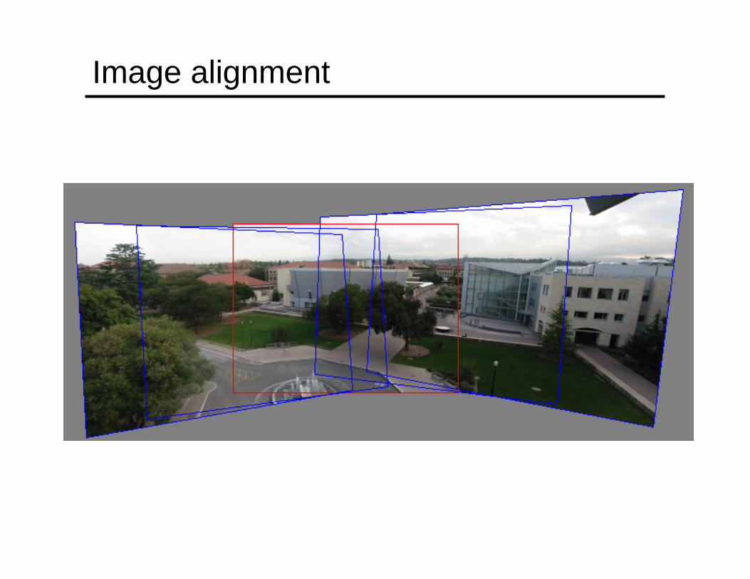
Image alignment
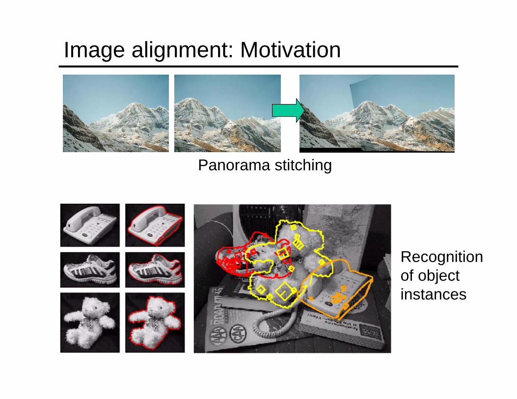
Image alignment: Motivation
Panorama stitching
Recognitionof objectinstances

Image alignment: Challenges
Small degree of overlap
Occlusion,clutter
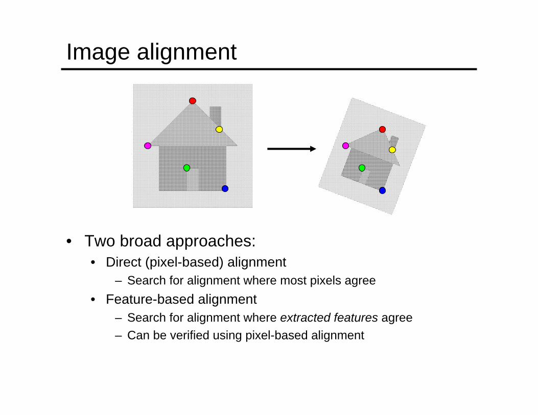
Image alignment
• Two broad approaches:• Direct (pixel-based) alignment
– Search for alignment where most pixels agree• Feature-based alignment
– Search for alignment where extracted features agree– Can be verified using pixel-based alignment
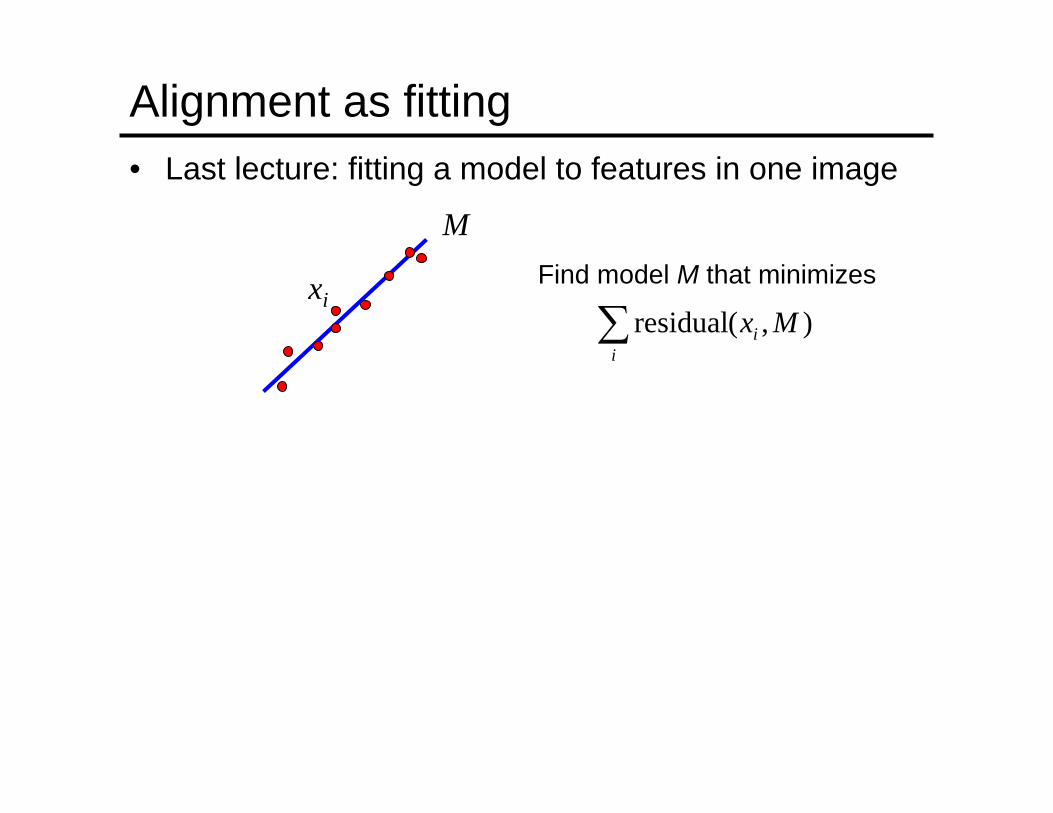
Alignment as fitting• Last lecture: fitting a model to features in one image
∑i
i Mx ),(residualFind model M that minimizes
M
xi
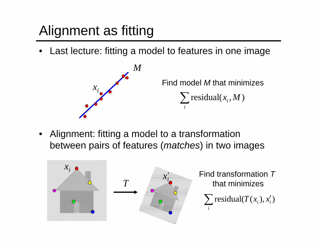
Alignment as fitting• Last lecture: fitting a model to features in one image
• Alignment: fitting a model to a transformation between pairs of features (matches) in two images
∑i
i Mx ),(residual
∑ ′i
ii xxT )),((residual
Find model M that minimizes
Find transformation Tthat minimizes
M
xi
T
xixi
'
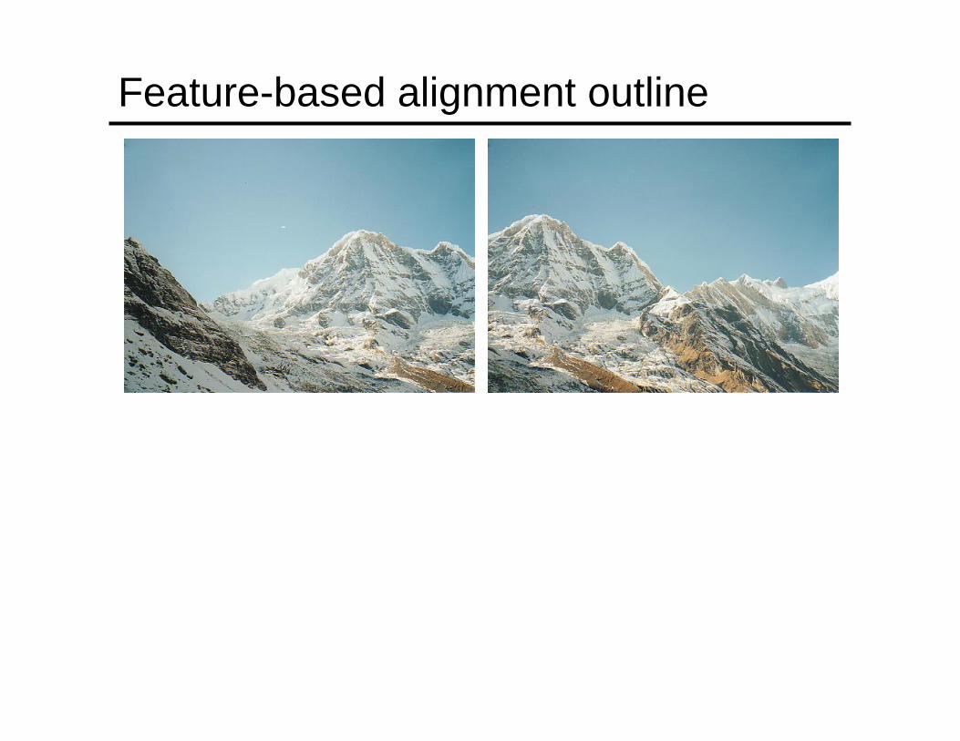
Feature-based alignment outline
Feature-based alignment outline
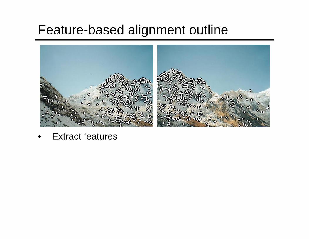
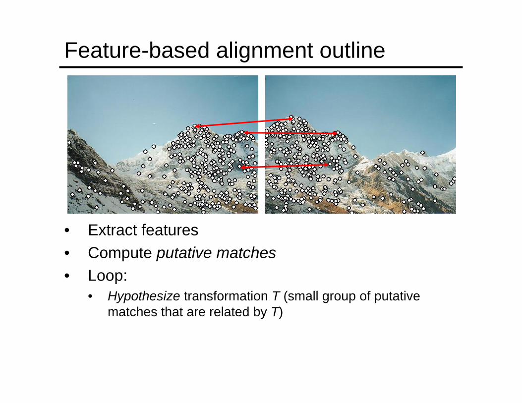
• Extract features
Feature-based alignment outline
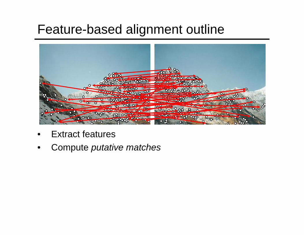
• Extract features• Compute putative matches
Feature-based alignment outline
• Extract features• Compute putative matches• Loop:
• Hypothesize transformation T (small group of putative matches that are related by T)

Feature-based alignment outline
• Extract features• Compute putative matches• Loop:
• Hypothesize transformation T (small group of putative matches that are related by T)
• Verify transformation (search for other matches consistent with T)

Feature-based alignment outline
• Extract features• Compute putative matches• Loop:
• Hypothesize transformation T (small group of putative matches that are related by T)
• Verify transformation (search for other matches consistent with T)

2D transformation models
• Similarity(translation, scale, rotation)
• Affine
• Projective(homography)
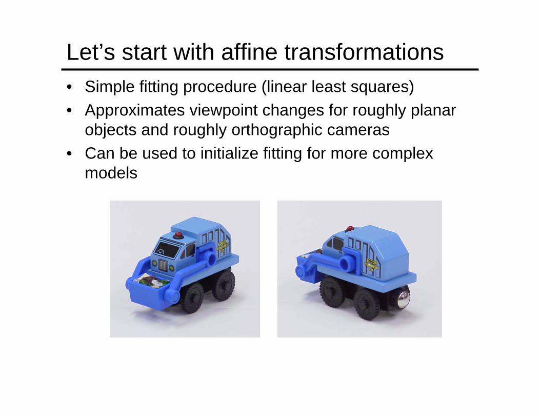
Let’s start with affine transformations• Simple fitting procedure (linear least squares)• Approximates viewpoint changes for roughly planar
objects and roughly orthographic cameras• Can be used to initialize fitting for more complex
models
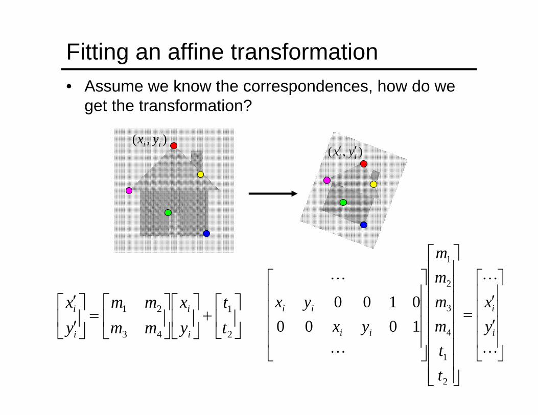
Fitting an affine transformation• Assume we know the correspondences, how do we
get the transformation?
),( ii yx ′′),( ii yx
⎥⎦
⎤⎢⎣
⎡+⎥
⎦
⎤⎢⎣
⎡⎥⎦
⎤⎢⎣
⎡=⎥
⎦
⎤⎢⎣
⎡′′
2
1
43
21
tt
yx
mmmm
yx
i
i
i
i
⎥⎥⎥⎥
⎦
⎤
⎢⎢⎢⎢
⎣
⎡
′′
=
⎥⎥⎥⎥⎥⎥⎥⎥
⎦
⎤
⎢⎢⎢⎢⎢⎢⎢⎢
⎣
⎡
⎥⎥⎥⎥
⎦
⎤
⎢⎢⎢⎢
⎣
⎡
L
L
L
L
i
i
ii
ii
yx
ttmmmm
yxyx
2
1
4
3
2
1
10000100

Fitting an affine transformation
• Linear system with six unknowns• Each match gives us two linearly independent
equations: need at least three to solve for the transformation parameters
⎥⎥⎥⎥
⎦
⎤
⎢⎢⎢⎢
⎣
⎡
′′
=
⎥⎥⎥⎥⎥⎥⎥⎥
⎦
⎤
⎢⎢⎢⎢⎢⎢⎢⎢
⎣
⎡
⎥⎥⎥⎥
⎦
⎤
⎢⎢⎢⎢
⎣
⎡
L
L
L
L
i
i
ii
ii
yx
ttmmmm
yxyx
2
1
4
3
2
1
10000100
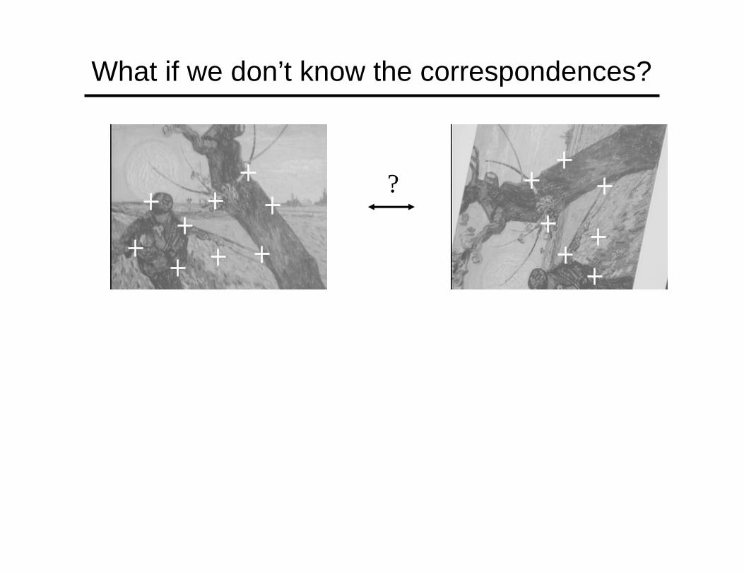
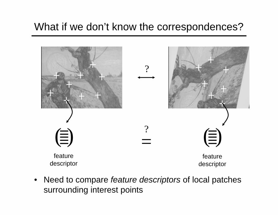
What if we don’t know the correspondences?
?
What if we don’t know the correspondences?
• Need to compare feature descriptors of local patches surrounding interest points
( ) ( )=?
featuredescriptor
featuredescriptor
?

Feature descriptors• Assuming the patches are already normalized (i.e.,
the local effect of the geometric transformation is factored out), how do we compute their similarity?
• Want invariance to intensity changes, noise, perceptually insignificant changes of the pixel pattern

• Simplest descriptor: vector of raw intensity values• How to compare two such vectors?
• Sum of squared differences (SSD)
– Not invariant to intensity change
• Normalized correlation
– Invariant to affine intensity change
Feature descriptors
( )∑ −=i
ii vuvu 2),SSD(
⎟⎟⎠
⎞⎜⎜⎝
⎛−⎟⎟
⎠
⎞⎜⎜⎝
⎛−
−−=
∑∑
∑
jj
jj
i ii
vvuu
vvuuvu
22 )()(
))((),(ρ
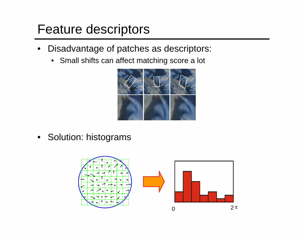
Feature descriptors• Disadvantage of patches as descriptors:
• Small shifts can affect matching score a lot
• Solution: histograms
0 2 π
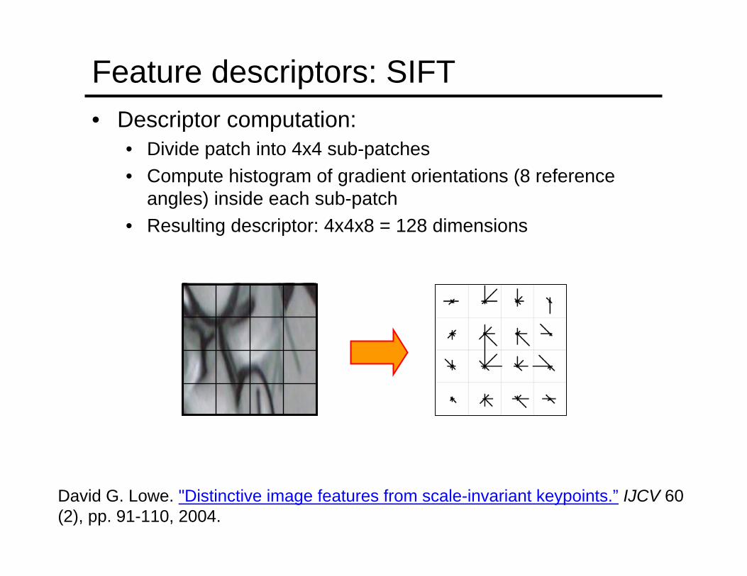
• Descriptor computation:• Divide patch into 4x4 sub-patches• Compute histogram of gradient orientations (8 reference
angles) inside each sub-patch• Resulting descriptor: 4x4x8 = 128 dimensions
Feature descriptors: SIFT
David G. Lowe. "Distinctive image features from scale-invariant keypoints.” IJCV 60 (2), pp. 91-110, 2004.

• Descriptor computation:• Divide patch into 4x4 sub-patches• Compute histogram of gradient orientations (8 reference
angles) inside each sub-patch• Resulting descriptor: 4x4x8 = 128 dimensions
• Advantage over raw vectors of pixel values• Gradients less sensitive to illumination change• “Subdivide and disorder” strategy achieves robustness to
small shifts, but still preserves some spatial information
Feature descriptors: SIFT
David G. Lowe. "Distinctive image features from scale-invariant keypoints.” IJCV 60 (2), pp. 91-110, 2004.

Feature matching
?
• Generating putative matches: for each patch in one image, find a short list of patches in the other image that could match it based solely on appearance

Feature matching• Generating putative matches: for each patch in one
image, find a short list of patches in the other image that could match it based solely on appearance• Exhaustive search
– For each feature in one image, compute the distance to allfeatures in the other image and find the “closest” ones (threshold or fixed number of top matches)
• Fast approximate nearest neighbor search– Hierarchical spatial data structures (kd-trees, vocabulary trees)– Hashing
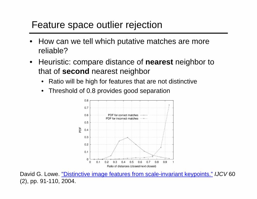
Feature space outlier rejection• How can we tell which putative matches are more
reliable?• Heuristic: compare distance of nearest neighbor to
that of second nearest neighbor• Ratio will be high for features that are not distinctive• Threshold of 0.8 provides good separation
David G. Lowe. "Distinctive image features from scale-invariant keypoints.” IJCV 60 (2), pp. 91-110, 2004.

Dealing with outliers• The set of putative matches still contains a very high
percentage of outliers• How do we fit a geometric transformation to a small
subset of all possible matches?• Possible strategies:
• RANSAC• Incremental alignment• Hough transform• Hashing

Strategy 1: RANSACRANSAC loop:1. Randomly select a seed group of matches2. Compute transformation from seed group3. Find inliers to this transformation 4. If the number of inliers is sufficiently large, re-compute
least-squares estimate of transformation on all of the inliers
Keep the transformation with the largest number of inliers

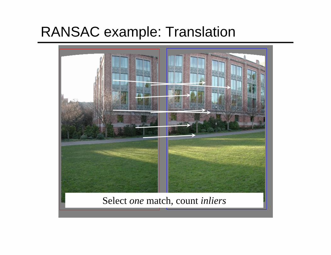
RANSAC example: Translation
Putative matches
RANSAC example: Translation
Select one match, count inliers

RANSAC example: Translation
Select one match, count inliers

RANSAC example: Translation
Find “average” translation vector

Problem with RANSAC• In many practical situations, the percentage of
outliers (incorrect putative matches) is often very high (90% or above)
• Alternative strategy: restrict search space by using strong locality constraints on seed groups and inliers• Incremental alignment
Strategy 2: Incremental alignment• Take advantage of strong locality constraints: only
pick close-by matches to start with, and gradually add more matches in the same neighborhood
S. Lazebnik, C. Schmid and J. Ponce, “Semi-local affine parts for object recognition,” BMVC 2004.

Strategy 2: Incremental alignment• Take advantage of strong locality constraints: only
pick close-by matches to start with, and gradually add more matches in the same neighborhood
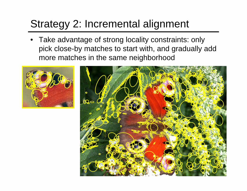
Strategy 2: Incremental alignment• Take advantage of strong locality constraints: only
pick close-by matches to start with, and gradually add more matches in the same neighborhood

Strategy 2: Incremental alignment• Take advantage of strong locality constraints: only
pick close-by matches to start with, and gradually add more matches in the same neighborhood
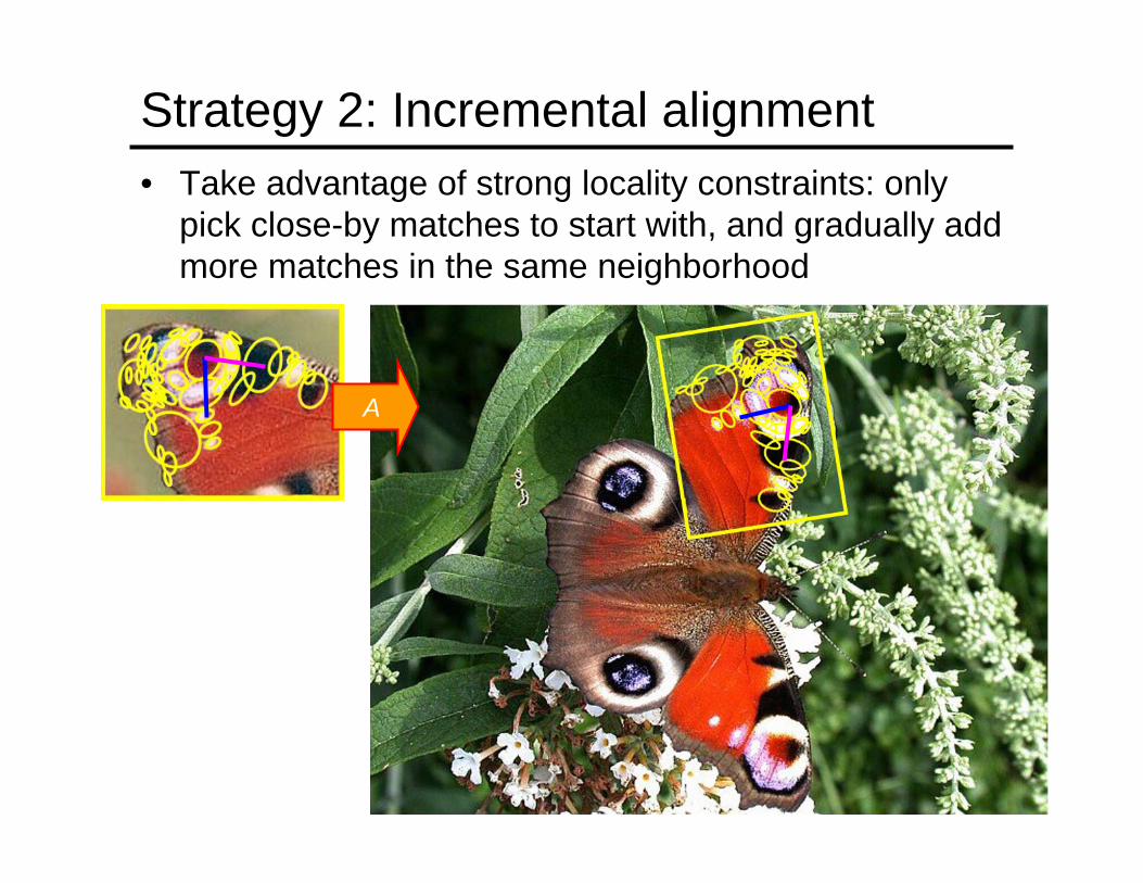
A
Strategy 2: Incremental alignment• Take advantage of strong locality constraints: only
pick close-by matches to start with, and gradually add more matches in the same neighborhood

Incremental alignment: Details
Generating seed groups:• Identify triples of neighboring features (i, j, k) in first image• Find all triples (i', j', k') in the second image such that i' (resp.
j', k') is a putative match of i (resp. j, k), and j', k' are neighbors of i'
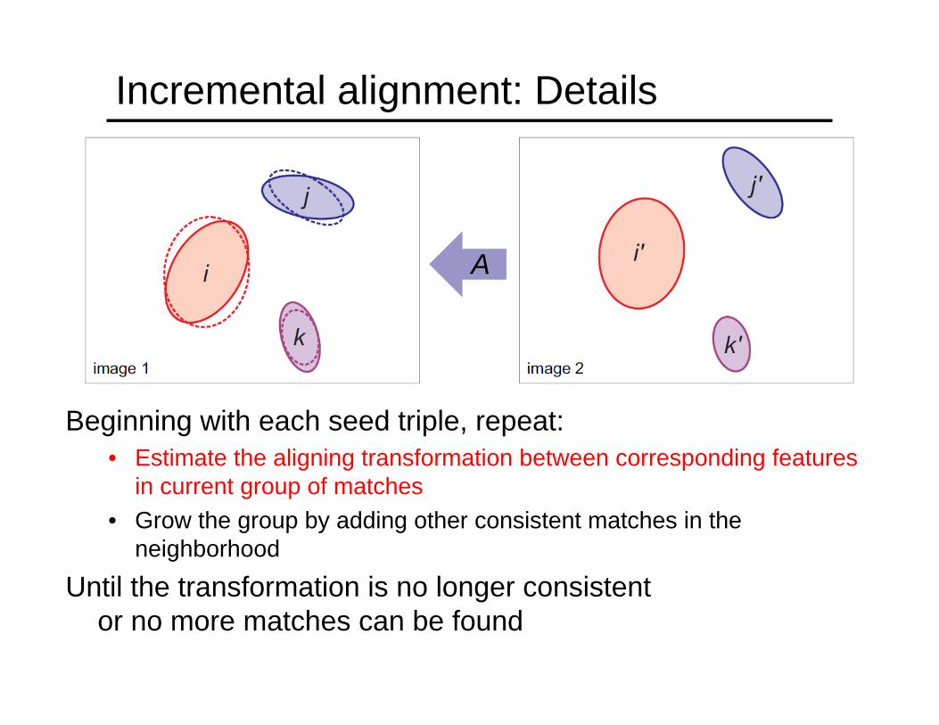
Incremental alignment: Details
Beginning with each seed triple, repeat:• Estimate the aligning transformation between corresponding features
in current group of matches• Grow the group by adding other consistent matches in the
neighborhood
Until the transformation is no longer consistent or no more matches can be found
A
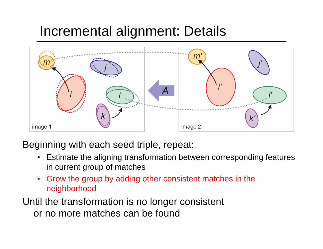
Incremental alignment: Details
A
Beginning with each seed triple, repeat:• Estimate the aligning transformation between corresponding features
in current group of matches• Grow the group by adding other consistent matches in the
neighborhood
Until the transformation is no longer consistent or no more matches can be found

Incremental alignment: Details
Beginning with each seed triple, repeat:• Estimate the aligning transformation between corresponding features
in current group of matches• Grow the group by adding other consistent matches in the
neighborhood
Until the transformation is no longer consistent or no more matches can be found
A'

Strategy 3: Hough transform• Suppose our features are scale- and rotation-invariant
• Then a single feature match provides an alignment hypothesis (translation, scale, orientation)
David G. Lowe. "Distinctive image features from scale-invariant keypoints.”IJCV 60 (2), pp. 91-110, 2004.
model

Strategy 3: Hough transform• Suppose our features are scale- and rotation-invariant
• Then a single feature match provides an alignment hypothesis (translation, scale, orientation)
• Of course, a hypothesis obtained from a single match is unreliable• Solution: let each match vote for its hypothesis in a Hough space
with very coarse bins
David G. Lowe. "Distinctive image features from scale-invariant keypoints.”IJCV 60 (2), pp. 91-110, 2004.
model
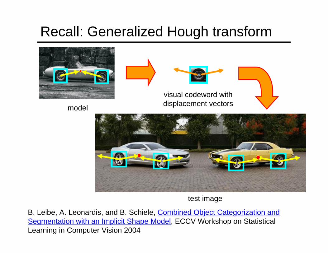
Recall: Generalized Hough transform
B. Leibe, A. Leonardis, and B. Schiele, Combined Object Categorization and Segmentation with an Implicit Shape Model, ECCV Workshop on Statistical Learning in Computer Vision 2004
model
visual codeword withdisplacement vectors
test image
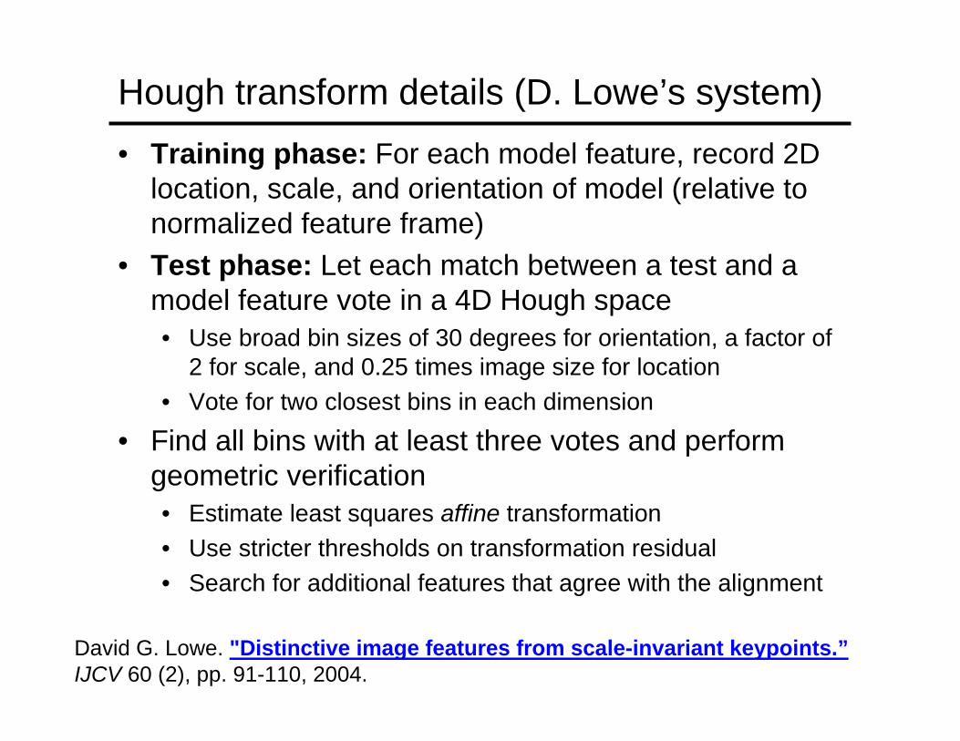
Hough transform details (D. Lowe’s system)• Training phase: For each model feature, record 2D
location, scale, and orientation of model (relative to normalized feature frame)
• Test phase: Let each match between a test and a model feature vote in a 4D Hough space• Use broad bin sizes of 30 degrees for orientation, a factor of
2 for scale, and 0.25 times image size for location• Vote for two closest bins in each dimension
• Find all bins with at least three votes and perform geometric verification • Estimate least squares affine transformation • Use stricter thresholds on transformation residual• Search for additional features that agree with the alignment
David G. Lowe. "Distinctive image features from scale-invariant keypoints.”IJCV 60 (2), pp. 91-110, 2004.

Image alignment: Review• What is the bias/variance tradeoff?• What are the advantages of a 2D affine alignment
model?• What are the main steps in feature-based alignment?• How do we generate putative matches?• How does the SIFT descriptor work?• What are different computational strategies for
estimating an alignment in the presence of outliers?• Strategy 1: RANSAC• Strategy 2: Incremental alignment• Strategy 3: Hough transform• Strategy 4: Hashing (next)

Strategy 4: Hashing• Make each invariant image feature into a low-dimensional “key”
that indexes into a table of hypotheses
model
hash table
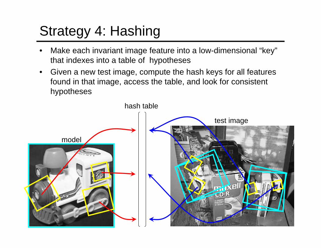
Strategy 4: Hashing• Make each invariant image feature into a low-dimensional “key”
that indexes into a table of hypotheses• Given a new test image, compute the hash keys for all features
found in that image, access the table, and look for consistent hypotheses
model
hash table
test image
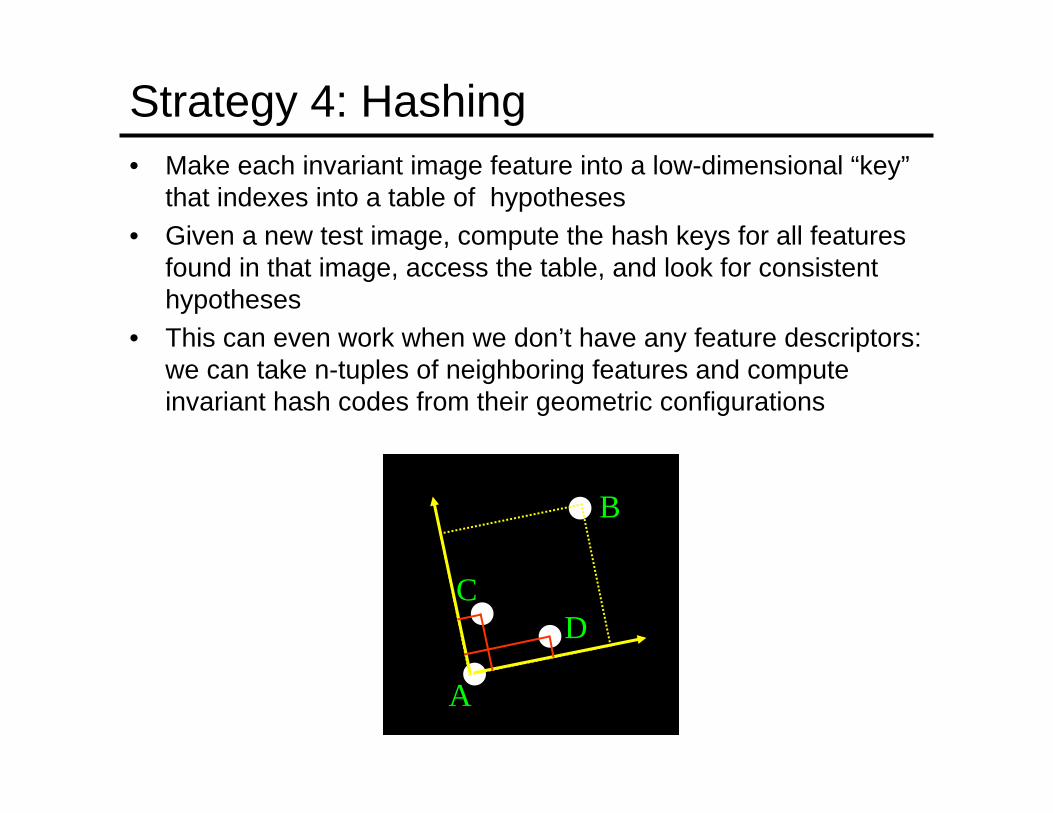
Strategy 4: Hashing• Make each invariant image feature into a low-dimensional “key”
that indexes into a table of hypotheses• Given a new test image, compute the hash keys for all features
found in that image, access the table, and look for consistent hypotheses
• This can even work when we don’t have any feature descriptors: we can take n-tuples of neighboring features and compute invariant hash codes from their geometric configurations
A
B
CD
Application: Searching the skyhttp://www.astrometry.net/
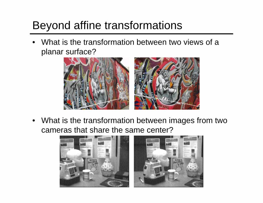
Beyond affine transformations• What is the transformation between two views of a
planar surface?
• What is the transformation between images from two cameras that share the same center?
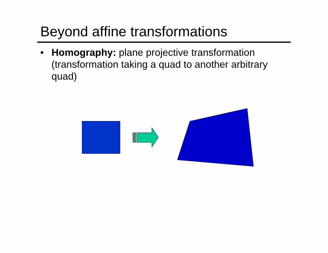
Beyond affine transformations• Homography: plane projective transformation
(transformation taking a quad to another arbitrary quad)

Fitting a homography• Recall: homogenenous coordinates
Converting to homogenenousimage coordinates
Converting from homogenenousimage coordinates

Fitting a homography• Recall: homogenenous coordinates
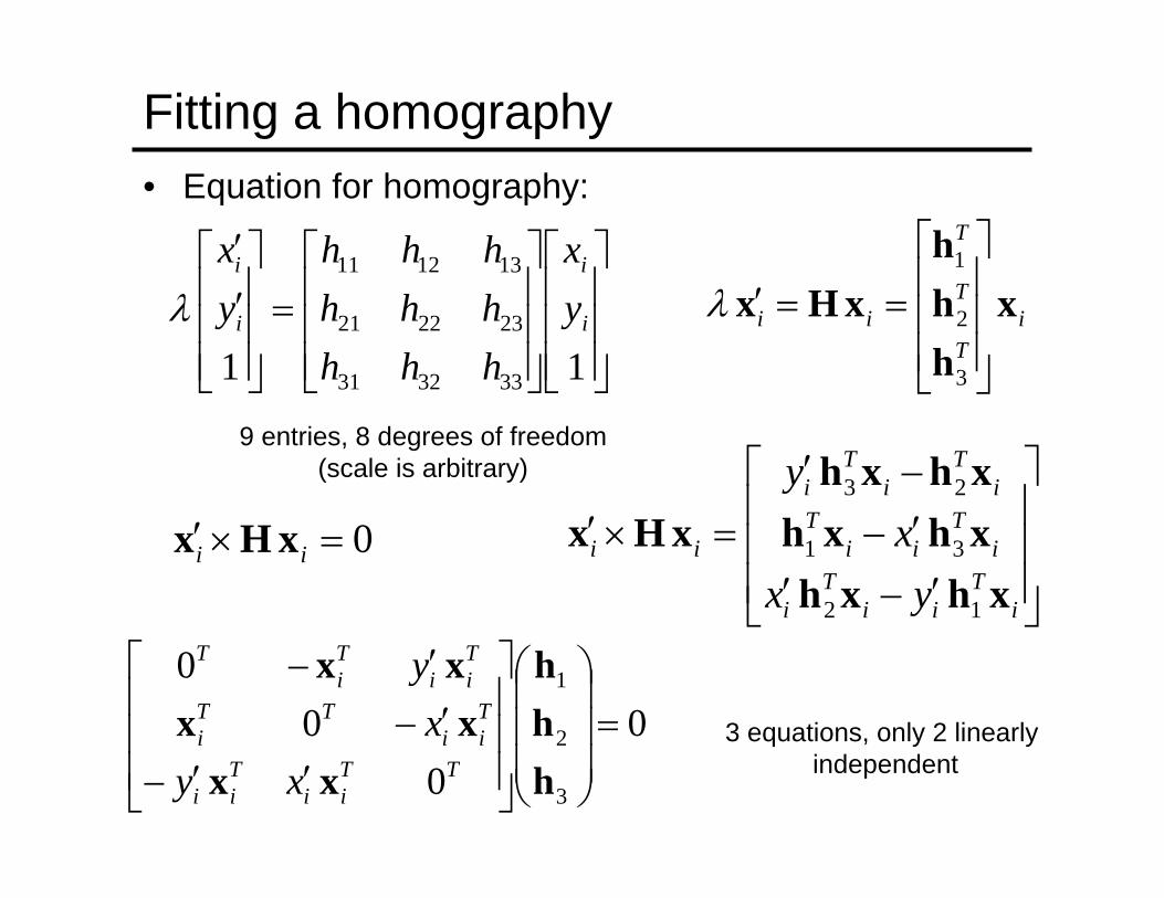
• Equation for homography:
Converting to homogenenousimage coordinates
Converting from homogenenousimage coordinates
⎥⎥⎥
⎦
⎤
⎢⎢⎢
⎣
⎡
⎥⎥⎥
⎦
⎤
⎢⎢⎢
⎣
⎡=
⎥⎥⎥
⎦
⎤
⎢⎢⎢
⎣
⎡′′
11 333231
232221
131211
yx
hhhhhhhhh
yx
λ
Fitting a homography• Equation for homography:
iT
T
T
ii xhhh
xHx⎥⎥⎥
⎦
⎤
⎢⎢⎢
⎣
⎡
==′
3
2
1
λ⎥⎥⎥
⎦
⎤
⎢⎢⎢
⎣
⎡
⎥⎥⎥
⎦
⎤
⎢⎢⎢
⎣
⎡=
⎥⎥⎥
⎦
⎤
⎢⎢⎢
⎣
⎡′′
11 333231
232221
131211
i
i
i
i
yx
hhhhhhhhh
yx
λ
0=×′ ii xHx⎥⎥⎥
⎦
⎤
⎢⎢⎢
⎣
⎡
′−′′−−′
=×′
iT
iiT
i
iT
iiT
iT
iT
i
ii
yxx
y
xhxhxhxhxhxh
xHx
12
31
23
00
00
3
2
1
=⎟⎟⎟
⎠
⎞
⎜⎜⎜
⎝
⎛
⎥⎥⎥
⎦
⎤
⎢⎢⎢
⎣
⎡
′′−
′−
′−
hhh
xxxx
xx
TTii
Tii
Tii
TTi
Tii
Ti
T
xyx
y
3 equations, only 2 linearly independent
9 entries, 8 degrees of freedom(scale is arbitrary)
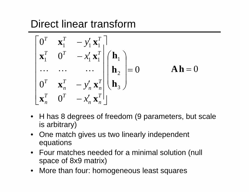
Direct linear transform
• H has 8 degrees of freedom (9 parameters, but scale is arbitrary)
• One match gives us two linearly independent equations
• Four matches needed for a minimal solution (null space of 8x9 matrix)
• More than four: homogeneous least squares
0
00
00
3
2
1111
111
=⎟⎟⎟
⎠
⎞
⎜⎜⎜
⎝
⎛
⎥⎥⎥⎥⎥⎥
⎦
⎤
⎢⎢⎢⎢⎢⎢
⎣
⎡
′−
′−
′−
′−
hhh
xxxx
xxxx
Tnn
TTn
Tnn
Tn
T
TTT
TTT
xy
xy
LLL 0=hA

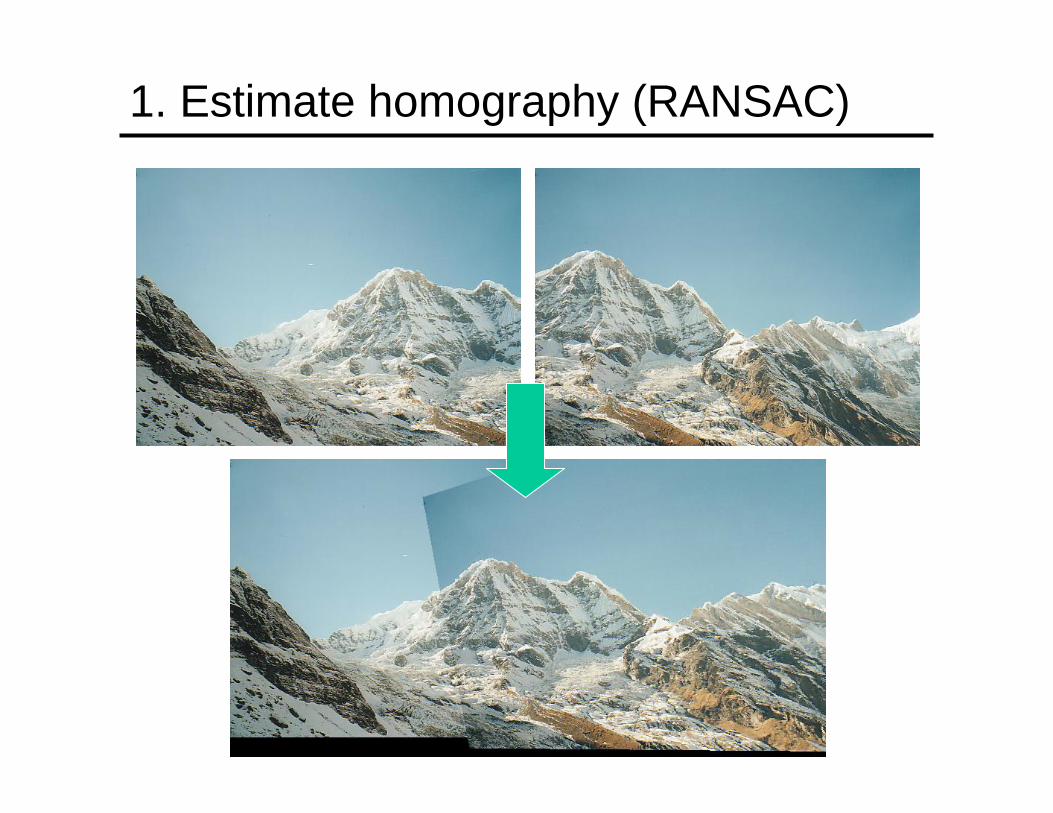
Application: Panorama stitching

Recognizing panoramas
M. Brown and D. Lowe, “Recognizing Panoramas,” ICCV 2003.
• Given contents of a camera memory card, automatically figure out which pictures go together and stitch them together into panoramas
http://www.cs.ubc.ca/~mbrown/panorama/panorama.html

1. Estimate homography (RANSAC)

1. Estimate homography (RANSAC)
1. Estimate homography (RANSAC)

2. Find connected sets of images
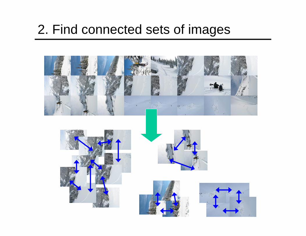
2. Find connected sets of images

2. Find connected sets of images
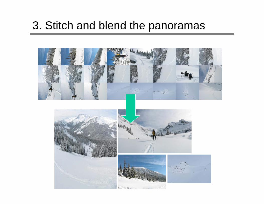
3. Stitch and blend the panoramas

Results
Issues in alignment-based applications
• Choosing the geometric alignment model• Tradeoff between “correctness” and robustness (also,
efficiency)
• Choosing the descriptor• “Rich” imagery (natural images): high-dimensional patch-based
descriptors (e.g., SIFT)• “Impoverished” imagery (e.g., star fields): need to create
invariant geometric descriptors from k-tuples of point-based features
• Strategy for finding putative matches• Small number of images, one-time computation (e.g., panorama
stitching): brute force search• Large database of model images, frequent queries: indexing or
hashing• Heuristics for feature-space pruning of putative matches

Issues in alignment-based applications
• Choosing the geometric alignment model• Choosing the descriptor• Strategy for finding putative matches• Hypothesis generation strategy
• Relatively large inlier ratio: RANSAC• Small inlier ratio: locality constraints, Hough transform
• Hypothesis verification strategy• Size of consensus set, residual tolerance depend on inlier ratio
and expected accuracy of the model• Possible refinement of geometric model• Dense verification
Next time: Single-view geometry
Top Related