


Languages
Pages
Legal

Published in Geomorphology 74, issues 1-4, 181-195, 2006which should be used for any reference to this work
1
Identification of facies models in alluvial soil formation:
The case of a Swiss alpine floodplain
G. Bullinger-Weber *, J.-M. Gobat
Laboratory Soil and Vegetation, University of Neuchatel, Emile-Argand 11, CH-2007 Neuchatel, Switzerland
Abstract
This paper describes different conceptual facies models intervening in alluvial soil formation in the case of the Sarine River
floodplain, a partially embanked floodplain situated in the northwest of the Swiss Alps. Alluvial soils are submitted to processes of
deposition and erosion and exhibit various characteristics reflecting the composition and properties of the material transported.
Moreover, these processes of sedimentation and erosion vary in space and time and contribute thus to the heterogeneity of the
whole floodplain system. Detailed analyses of the different soil layers permit a precise description of the variability and complexity
of soil formation. In addition, the vertical succession of the horizons is useful to reconstruct the different natural or artificial events
that occurred in this alluvial valley since the nineteenth century. On a larger scale, this study aims to contribute to floodplain
management by identifying zones for restoration. The investigation was undertaken using data from 109 auger borings carried out
in the Sarine River valley. Several morphological attributes of the different horizons and of the different profiles were first reduced
in number and then grouped by a hierarchical agglomerative clustering. Profile factors were analysed by means of correlation
analyses as well as other data summaries. The results showed positive correlations between several factors, particularly between the
total profile thickness and the number of horizons found in the profile. Four facies models of alluvial soil formation are then
proposed to illustrate and explain the variability of alluvial soil formation in the Sarine floodplain. Finally, these facies models are
placed into the context of the Sarine floodplain scale case, according to the levels of organization of the alluvial system.
Keywords: Facies models; Alluvial soil; Soil formation; Hierarchical levels; Floodplain; Switzerland
1. Introduction
Floodplains are ecotones forming a transition be-
tween aquatic and terrestrial environments. They are
characterized by complex ecological systems and are
dynamic spatial mosaics, more or less connected with
the active channel of the river. These lateral connections
*Corresponding author. Tel.: +41 32 71822 20; fax: +41 32 7182231.
E-mail address: [email protected] (G. Bullinger-Weber).
are essential for the functioning and integrity of a
floodplain (Thoms, 2003), and the various landscape
patches induce a hierarchical system that can be con-
sidered at different levels. Thoms (2003) also reported
that many floodplain management strategies often fail
to provide scientific knowledge at the appropriate scale.
The approach described by Petts and Amoros (1996) is
based on the fluvial hydrosystem. This one is defined as
an eco-complex forming by different environments that
are dependent to a greater or lesser degree on connec-
tivity with the active channel of the river, just like the
character of this main channel also depends on interac-

2
tions with those environments. In other words, the
fluvial hydrosystem may be viewed as a nested hierar-
chy of subsystems with different levels controlled by
different rates and types of processes. Five distinct
levels are then described:
– the drainage basin, delineated by a topographic di-
vide (the watershed) that results from geological
processes and climatic changes;
– the functional sectors, delimited by changes in valley
width and gradient due to different flow, water-quali-
ty and sediment regimes draining subbasins of dif-
ferent geological, climatic and biogeographical
character;
– the functional sets, defined as sections of typical
ecological units associated with specific landforms
(e.g. major cutoff meander, aggrading floodplain,
main channel);
– functional units, characterized by a typical animal
and plant community that is indicative of the habitat
conditions at the site that are generally arranged in
spatial successions along topographic gradients; and
– the mesohabitats, subdivisions of functional unit that
are particularly sensitive to variations of the control
variables and may change from year to year.
The integrity of the fluvial hydrosystem depends
then on the dynamic interaction between hydrological,
geomorphological, and biological processes. The explo-
ration and analysis of the multivariate and spatial data
found in these ecological attributes of floodplains are
commonly explored by standard methods such as cor-
respondence analysis or clustering and are widely used
by ecologists.
In this complex ecological system, alluvial soils are
characterized by sediment transport and deposition, as
well as by soil formation (Gerrard, 1987), and could be
identified at the level of functional units. In fact, these
particular sequences evolve from a single origin by
progressive changes over time-scales of 10�1 to 102
years and the processes involved include sedimentation
or organic matter accumulation for example (Petts and
Amoros, 1996). Thus, this combination of geomorphic
and pedologic processes is the main property of allu-
vial soils providing good elements for the interpretation
of past environmental changes (Daniels, 2003). More-
over, alluvial soil morphology varies according to
landscape position and overbank lithofacies (Autin
and Aslan, 2001), but also from river modifications
through time, such as embankments and dam construc-
tions. These geomorphic processes produce a land-
scape mosaic reflected by abrupt juxtapositions of
soils of different ages and degrees of profile develop-
ment (McAuliffe, 1994).
Stratification, formed by the alternation of pedologi-
cal layers and layers with new material, is a particular
characteristic of alluvial soils (Gerrard, 1987). New
deposition may bury a pre-existing soil and move it
away from the zone of active pedogenesis (Daniels,
2003). Alluvial soils are good models to estimate the
part of pedogenesis illustrating periods of stability with
development of pedogenic features and pedoturbation,
representing the overlay of sediments or instability
periods (Paton et al., 1995) in high or low energy
depositional environments. High energy deposition
contains coarse sediment deposited by traction currents,
whereas low energy deposition is characterised by fine-
grain sediment deposited by suspension settling.
The process of soil cumulization is particularly im-
portant in a floodplain context because all floodplains
are subject to pedogenesis during the intervals between
periods of sediment deposition. These vertical succes-
sions of overbank deposits and pedogenic features are
defined as paleosols by Kraus and Brown (1988) and
are generated by slow and sporadic aggradation and soil
modification interrupted by more rapid deposition.
Paleosols can be identified as buried soils determined
by five groups of soil-forming factors: climate, or-
ganisms (including man), relief, parent material, and
time (Bronger and Catt, 1998). They can also be
regarded as polygenetic soils if they contain features
formed during two or more periods of different envi-
ronmental conditions and they demonstrate moreover
an inverse relationship between soil maturity and sedi-
ment accumulation. But, paleosols are not restricted to
alluvial context, so the term pedofacies is mainly pre-
ferred in order to delimit the lateral changes of adjacent
packages of sedimentation rock when they vary in their
ancient soil properties as a function of their distance
from areas of relatively high sediment accumulation
(Kraus and Brown, 1988). According to these last
authors, the concept of pedogenic maturity is used to
infer sediment accumulation rates at different locations
in ancient floodplain environments: weak soil develop-
ment is assumed where sedimentation rates are rapid
and strong development is presumed where sediment
accumulation is slow. In a semiarid cut-and-fill flood-
plain context, Daniels (2003) defined three alluvial
pedofacies. These three identical soils are shown to
have developed different pedogenic features through
time as a result of different aggradation rates. Daniels
(2003) also defined A horizons as soil-stratigraphic
markers and indicators of relative aggradation rates.
Thus, identification of the different horizons present
3
in a soil, reflecting different aggradation phenomena
due to floods or development of a weak soil structure,
seems to be the ideal level approach to describe pre-
cisely the variability and complexity of the alluvial soil
profiles. The conceptual models of facies may then be
adapted and used in other floodplain context, such as
embanked zones. In these particular damaged systems,
the lateral connectivity is broken resulting in a quasi
complete isolation of the river from its floodplain and in
a suspension of aggradation. Embanked river floodplain
deposits are lithologically and sedimentologically dif-
ferent from natural (not human-influenced) floodplain
deposits and only pedogenic characteristics are then
observed in the subsurface of paleosols.
Using the concept of pedofacies defined by Kraus
and Brown (1988) on the basis of differences in paleo-
sol development, this study aims to develop a similar
hierarchy—or similar facies models—including the lat-
eral and vertical changes of soil development at dif-
ferent spatial and temporal scales in the case of the
embanked Sarine River floodplain. As embanked rivers
represent a large part of the actual floodplain cases, at
least in Europe, a better comprehension of the aggra-
dation and soil formation processes in the soils that are
now disconnected from the current flow, as well as a
better knowledge of their spatial distribution along the
riparian corridor, is highly relevant to understand the
global functioning of the Sarine River floodplain. In
order to undertake a detailed examination of these
properties, the vertical succession of the horizons (as
defined by Gerrard, 2000), presenting pedogenic fea-
tures or consisting of overbank sediments, were used to
describe the stratification of different alluvial soils at
functional set and unit levels according to Petts and
Amoros (1996). As these different sequences could be
related to the concepts primarily used in ecological
research (fluvial hydrosystem), analysis commonly
used in ecology is appropriate in our context of pedo-
logy and geomorphology. Results from this research,
giving abstract categories and statistical abstractions of
soil properties, are then employed to establish modified
simple conceptual models of alluvial soil formation
used for describing in a rapid, simple, and inexpensive
way the soils of the Sarine floodplain. These methods
are then compared with other soil classifications or soil
survey methods practiced in pedology. Simple indica-
tors, mainly horizon and soil profiles parameters (e.g.,
thickness of horizons, soil texture as defined in field;
Gobat et al., 2004), were used in order to identify the
different mechanisms for floodplain soil formation and
to understand the landscape evolution of an alpine
floodplain altered by human activity.
2. Materials and methods
2.1. Study area description
The Sarine River is situated in the NW of the Swiss
Alps (canton Fribourg) and is a tributary of the Aare
River, which flows into the Rhine River (Fig. 1). The
length of the study section is 12 km between Lessoc
(770 m) and the Gruyere Lake near Broc (670 m) with
an average slope of 0.0006 m m�1. The hydrological
regime is an intermediate nival regime with a maximum
flow in spring and a minimum flow in January. The
catchment area covers 639 km2 with an average altitude
of 1520 m. From 1972 to 2001, the maximum annual
peak discharge was 400 m3/s in 1974, and the mean
annual discharge was 217 m3/s.
The geomorphology of the section is characterized
by a succession of alluvial basins separated by rocky
constrictions, and the deposits are calcareous (Men-
donca Santos et al., 1997). But some geomorpholo-
gical particularities are observed. For example, the
sites 1 and 2 (see (A) in Fig. 1) were formed, before
the construction of the Rossens dam and the formation
of the Gruyere Lake in 1948, of gravel bars colonized
by pioneer annual herb communities or willow shrubs
that covered the entire base bed of that part of the
valley. Nowadays, and despite an artificial origin, this
area is characterized by a dynamic system of slow
velocity river and lake environments with slow sedi-
mentation. Site 3 was considered before the embank-
ments as a blakeQ where regular floods appeared. This
section is constituted of flat fields laid on a gravel
substrate. About the upstream area, the site 4 (see (C)
in Fig. 1) is situated on gravel bars that have been
colonized by willow shrubs for about 20 years. Dif-
ferences in micro-geomorphology are visible inside
that site: natural levees and channel fills. The site 5
is also located in a natural environment but colonized
by tree population for 20 to 100 years. Micro-geomor-
phological conditions are also contained inside the
site: natural levees, channel fills, active or abandoned
channel fills. Site 6 is situated under a mature forest
but with different morphological characteristics such
as abandoned channel fills and natural levees. Sites 7
and 8 are closed to the river main channel and do not
show any particular features. All the sites are situated
on the first terrace that is only a few meters above
river level (from 50 cm to 2 m) and a distance of few
meters to about 100 m from the main river channel.
The total thickness above basal gravel varies slightly
throughout the study area but these variations should
not interfere in the results.

Fig. 1. Localisation of the Sarine floodplain with two major study areas: (A) downstream area with investigated zones in black (sites 1 to 3); (B)
location and distribution of embankments throughout the downstream area; (C) upstream area with investigated zones in black (sites 4 to 8); (D)
location and distribution of embankments built from 1917 to 1938 (and even to 1974) throughout the upstream area (distribution not exhaustive
because of missing archives). Cross: Swiss coordinate system (in km) for orientation.
4

5
Historical descriptions revealed that because of the
catastrophic flood of 1913, important engineering and
regulation works were necessary to strengthen the Sa-
rine riverbanks (Guex et al., 2003). Thus, a general
diking and canalisation with one pair of continuous
and unsinkable dikes were made to transform the braid-
ed channel system to a single uniform channel (Fig. 1).
Further embankment projects were undertaken during
the twentieth century to reconstruct the damaged struc-
tures and to build new structures, but sometimes and
particularly in the upstream area (part D) in Fig. 1), the
archives miss that makes difficult to recall the real
embankment history of the zone. These works progres-
sively caused the modification of the sedimentation–
erosion phenomena by interrupting the flooding and
disconnected the Sarine River from its floodplain.
Moreover, the creation of the Gruyere retention lake
in 1948 caused the nearly complete disappearance of a
very dynamic floodplain, except for a reduced area
close to Broc and a second one upstream near Grand-
villard situated in the two major study areas (Fig. 1).
After 1960, two main human activities related to
river systems, gravel mining and water retention by
dams in the upper catchments, increased the bed inci-
sion and the disconnection of the river from its flood-
plain. Between 1960 and 1976, gravel was removed
directly from the riverbed, and the combination of this
activity with the sediment retention upstream acceler-
ated the riverbed incision process already initiated by
the systematic river embanking.
2.2. Data acquisition
Alluvial soils of the Sarine floodplain were surveyed
by a detailed description of the morphology of different
core samplings throughout the two major study areas
(investigated zones (A) and (C) in Fig. 1). They were
identified according to the World Reference Base of
Soil Resources (ISSS/ISRIC/FAO, 1998) using soil
characteristics, properties and horizons. Soil characte-
ristics, as well as soil properties, were measured in the
field and emphasis was on describing the soil texture
characteristics of the deposited sediments and the pedo-
genic layers, but the pedogenic features were also
observed. The different layers were called horizons
(corresponding to the diagnostic horizons or reference
horizons; AFES, 1998), which are three-dimensional
bodies more or less parallel to the earth’s surface,
characterized by one or more properties and a variable
thickness. Their succession was named soil profile (or
profile), by analogy with soil science concepts, and
defined the sequence of information related to a
solum ordered from the land surface downwards
(AFES, 1998).
A total of 143 points were surveyed with a pedo-
logical auger; and 109 of them, the ones reaching the
basal calcareous gravels, were taken into consideration.
This limit was chosen because it represents the bottom
of the studied system and was considered as almost
similar throughout the study area. This sampling tech-
nique is commonly used to provide an indication of the
soils represented in the field and to describe the soil
types, if soil profiles have been previously determined
(Cosandey et al., 2003; Earl et al., 2003; Bragato,
2004). This is the case for this site where previous
studies have already been published (Bureau et al.,
1995; Fierz et al., 1995; Mendonca Santos et al.,
2000). The sediment cores were collected from repre-
sentative locations and identified as being uncultivated
and susceptible to regular overbank flooding (forests,
active zones), as well as cultivated and disconnected
from the river (agricultural and embanked zones). In
addition to precise geographical information and short
vegetation description, the following characteristics and
properties were recorded for each point:
(i) total thickness of the profile, from top surface to
pebble limit (cm);
(ii) number of horizons found in the profile;
(iii) depth (cm), thickness (cm), and texture of each
horizon; horizon thickness is considered in the
case of alluvial soils as a feature that can be
linked to the duration and intensity of floods;
the texture was identified by hand in the field; a
total of 367 horizons were described;
(iv) presence or absence of oxidation marks, of coarse
material (gravel and pebbles N2 mm), and of
organic macrorestes in each horizon; and
(v) soil structure of the topsoil horizon (e.g. particu-
lar, granular; Gobat et al., 2004) illustrating the
actual development of the soil.
In addition to these descriptive factors, two indexes
were calculated for each soil profile, namely the num-
ber of horizons per total thickness (named nb/thick in
Fig. 3) and the number of horizons per meter (nb/m in
Fig. 3). All these data were introduced into a database
to be studied and analysed.
2.3. Statistical analyses
The different attributes describing each horizon and
profile were separated for statistical analysis. Horizon
attributes were quantitative (depth and thickness), bi-
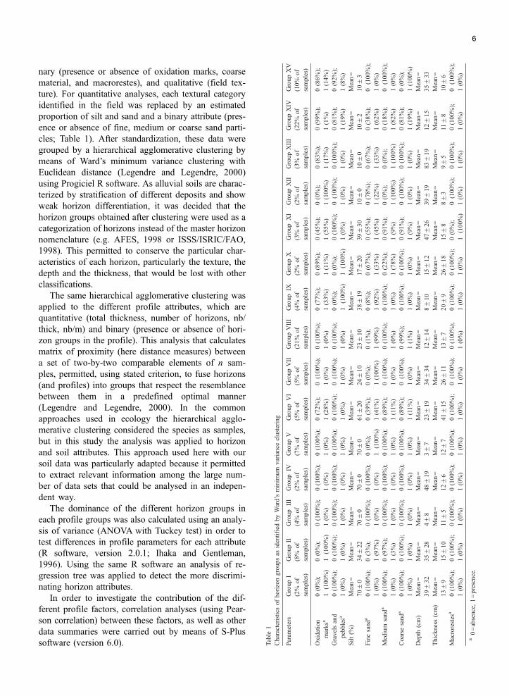
Table
1
Characteristicsofhorizongroupsas
identified
byWard’s
minim
um
variance
clustering
Param
eters
GroupI
(2%
of
samples)
GroupII
(8%
of
samples)
Group
III
(4%
of
samples)
GroupIV
(2%
of
samples)
GroupV
(7%
of
samples)
GroupVI
(5%
of
samples)
GroupVII
(5%
of
samples)
GroupVIII
(21%
of
samples)
GroupIX
(4%
of
samples)
GroupX
(2%
of
samples)
Group
XI
(3%
of
samples)
GroupXII
(2%
of
samples)
GroupXIII
(3%
of
samples)
GroupXIV
(22%
of
samples)
GroupXV
(10%
of
samples)
Oxidation
marksa
0(0%);
1(100%)
0(0%);
1(100%)
0(100%);
1(0%)
0(100%);
1(0%)
0(100%);
1(0%)
0(72%);
1(28%)
0(100%);
1(0%)
0(100%);
1(0%)
0(77%);
1(33%)
0(89%);
1(11%)
0(45%);
1(55%)
0(0%);
1(100%)
0(83%);
1(17%)
0(99%);
1(1%)
0(86%);
1(14%)
Gravelsand
pebblesa
0(100%);
1(0%)
0(100%);
1(0%)
0(100%);
1(0%)
0(100%);
1(0%)
0(100%);
1(0%)
0(100%);
1(0%)
0(100%);
1(0%)
0(100%);
1(0%)
0(0%);
1(100%)
0(0%);
1(100%)
0(100%);
1(0%)
0(100%);
1(0%)
0(100%);
1(0%)
0(81%);
1(19%)
0(92%);
1(8%)
Silt(%
)Mean=
70F0
Mean=
34F22
Mean=
70F0
Mean=
70F0
Mean=
70F0
Mean=
61F20
Mean=
24F10
Mean=
23F10
Mean=
38F19
Mean=
17F20
Mean=
39F30
Mean=
10F0
Mean=
10F0
Mean=
10F2
Mean=
10F3
Finesanda
0(100%);
1(0%)
0(3%);
1(97%)
0(100%);
1(0%)
0(100%);
1(0%)
0(0%);
1(100%)
0(39%);
1(41%)
0(0%);
1(100%)
0(1%);
1(99%)
0(8%);
1(92%)
0(67%);
1(33%)
0(55%);
1(45%)
0(78%);
1(22%)
0(67%);
1(33%)
0(38%);
1(62%)
0(100%);
1(0%)
Medium
sanda
0(100%);
1(0%)
0(97%);
1(3%)
0(100%);
1(0%)
0(100%);
1(0%)
0(100%);
1(0%)
0(89%);
1(11%)
0(100%);
1(0%)
0(100%);
1(0%)
0(100%);
1(0%)
0(22%);
1(78%)
0(91%);
1(9%)
0(0%);
1(100%)
0(0%);
1(100%)
0(18%);
1(82%)
0(100%);
1(0%)
Coarse
sanda
0(100%);
1(0%)
0(100%);
1(0%)
0(100%);
1(0%)
0(100%);
1(0%)
0(100%);
1(0%)
0(89%);
1(11%)
0(100%);
1(0%)
0(99%);
1(1%)
0(100%);
1(0%)
0(100%);
1(0%)
0(91%);
1(9%)
0(100%);
1(0%)
0(100%);
1(0%)
0(81%);
1(19%)
0(0%);
1(100%)
Depth
(cm)
Mean=
39F32
Mean=
35F28
Mean=
4F8
Mean=
48F19
Mean=
3F7
Mean=
23F19
Mean=
34F34
Mean=
12F14
Mean=
8F10
Mean=
15F12
Mean=
47F26
Mean=
39F19
Mean=
83F19
Mean=
12F15
Mean=
35F33
Thickness(cm)
Mean=
13F9
Mean=
15F10
Mean=
11F5
Mean=
12F6
Mean=
12F7
Mean=
41F15
Mean=
26F11
Mean=
13F7
Mean=
20F9
Mean=
26F18
Mean=
15F8
Mean=
8F3
Mean=
9F5
Mean=
11F8
Mean=
10F6
Macrorestes
a0(100%);
1(0%)
0(100%);
1(0%)
0(100%);
1(0%)
0(100%);
1(0%)
0(100%);
1(0%)
0(100%);
1(0%)
0(100%);
1(0%)
0(100%);
1(0%)
0(100%);
1(0%)
0(100%);
1(0%)
0(0%);
1(100%)
0(100%);
1(0%)
0(100%);
1(0%)
0(100%);
1(0%)
0(100%);
1(0%)
a0=absence,1=presence.
6
nary (presence or absence of oxidation marks, coarse
material, and macrorestes), and qualitative (field tex-
ture). For quantitative analyses, each textural category
identified in the field was replaced by an estimated
proportion of silt and sand and a binary attribute (pres-
ence or absence of fine, medium or coarse sand parti-
cles; Table 1). After standardization, these data were
grouped by a hierarchical agglomerative clustering by
means of Ward’s minimum variance clustering with
Euclidean distance (Legendre and Legendre, 2000)
using Progiciel R software. As alluvial soils are charac-
terized by stratification of different deposits and show
weak horizon differentiation, it was decided that the
horizon groups obtained after clustering were used as a
categorization of horizons instead of the master horizon
nomenclature (e.g. AFES, 1998 or ISSS/ISRIC/FAO,
1998). This permitted to conserve the particular char-
acteristics of each horizon, particularly the texture, the
depth and the thickness, that would be lost with other
classifications.
The same hierarchical agglomerative clustering was
applied to the different profile attributes, which are
quantitative (total thickness, number of horizons, nb/
thick, nb/m) and binary (presence or absence of hori-
zon groups in the profile). This analysis that calculates
matrix of proximity (here distance measures) between
a set of two-by-two comparable elements of n sam-
ples, permitted, using stated criterion, to fuse horizons
(and profiles) into groups that respect the resemblance
between them in a predefined optimal manner
(Legendre and Legendre, 2000). In the common
approaches used in ecology the hierarchical agglo-
merative clustering considered the species as samples,
but in this study the analysis was applied to horizon
and soil attributes. This approach used here with our
soil data was particularly adapted because it permitted
to extract relevant information among the large num-
ber of data sets that could be analysed in an indepen-
dent way.
The dominance of the different horizon groups in
each profile groups was also calculated using an analy-
sis of variance (ANOVA with Tuckey test) in order to
test differences in profile parameters for each attribute
(R software, version 2.0.1; Ihaka and Gentleman,
1996). Using the same R software an analysis of re-
gression tree was applied to detect the more discrimi-
nating horizon attributes.
In order to investigate the contribution of the dif-
ferent profile factors, correlation analyses (using Pear-
son correlation) between these factors, as well as other
data summaries were carried out by means of S-Plus
software (version 6.0).

7
3. Results
The soils have been identified as calcareous polyge-
netic Fluvisol or as Gleysol due to the World Reference
Base of Soil Resources (ISSS/ISRIC/FAO, 1998). The
clustering separates 15 groups of horizons (named
group I to group XV; Table 1, Fig. 2) and then 10 groups
of profiles (group 1 to group 10; Fig. 3).
Horizon groups differ from each other principally in
their texture parameter (from medium and coarse sand
to fine silt; Fig. 2), and then in their thickness com-
bined with the oxidation marks. Note that an absence
of oxidation marks does not mean that there is no
oxidation–reduction phenomenon, but only that these
marks were not visible at the moment of field observa-
tion or that particle size was too coarse for preservation.
Group I consists of very thin layers with oxidation
marks. Group II also presents oxidation marks, with a
coarser silty sandy texture. Groups III, IV, and V are
siltier and do not show any oxidation marks; they differ
on the basis of mean depth. Group VI is an intermediate
case between these last three groups. The fine sandy
textural horizons are represented by groups VII and
VIII, which also do not show any oxidation marks.
The presence of gravels is illustrated in groups IX
and X, but the particle size varies: fine sand for IX
and medium sand for X. Group XI is characterized by
various soil texture distributions but always with the
presence of macrorestes. Oxidation marks and medium
sand define group XII, whereas groups XIII and XIV
are only characterized by medium sand; the depth of
Fig. 2. Simplified dendrogram for 367 soil horizons obtained by means of
from the Sarine floodplain. The group fusion level is defined by a distance
tree in R Software version 2.0.1. Some horizon groups could appear twice o
this figure boxQ or boxmarksQ means oxidation marks).
each horizon differentiates these two groups. Coarse
sand with very little silt differentiates group XV from
all the others, independently of the other factors.
Topsoil horizon structure is mostly granular and
particular (63% and 25% of the horizons respectively).
The granular horizons are mainly represented by hori-
zons of group VIII (26%), group V (25%) and group
XIV (22%). Most of the particular horizons are found in
group XIV (63%) corresponding to a medium sandy
texture. The thickness of those topsoil horizons are
various (1 to 37 cm) but is generally thicker for the
granular horizons than for the particular ones (mean of
12 and 8 cm respectively).
Profile groups are separated by the factors of total
thickness (28 to 97 cm) and number of horizons (2 to
6.5; Fig. 3). Relative location of different groups within
the floodplain landscape is shown in Fig. 4. In this last
figure, the distribution of abstract representations of
real soil profiles is illustrated and does not necessarily
correspond to any of the 109 real profiles. Groups 1 to 5
are quite similar but differ from each other by the
parameter of the dominant horizons. They reveal pro-
files with few horizons and are not very thick. Group 1
differs from the other groups by a dominant presence of
horizons of group XV. Group 2 generally shows pro-
files with one or more horizons of group XIV and VIII,
which are also typical of group 3. Most of the profiles
are found in this last group where intermediate values
are observed between groups 1–2 and 4, except for the
number of horizons (1 to 4). Group 5 is characterized
by various total thicknesses (but thicker than groups 1
Ward’s minimum variance clustering and described in the 109 profiles
and the discriminating horizon attributes are obtained after a regression
r not at all in the dendrogram. See Table 1 for parameter designation (in
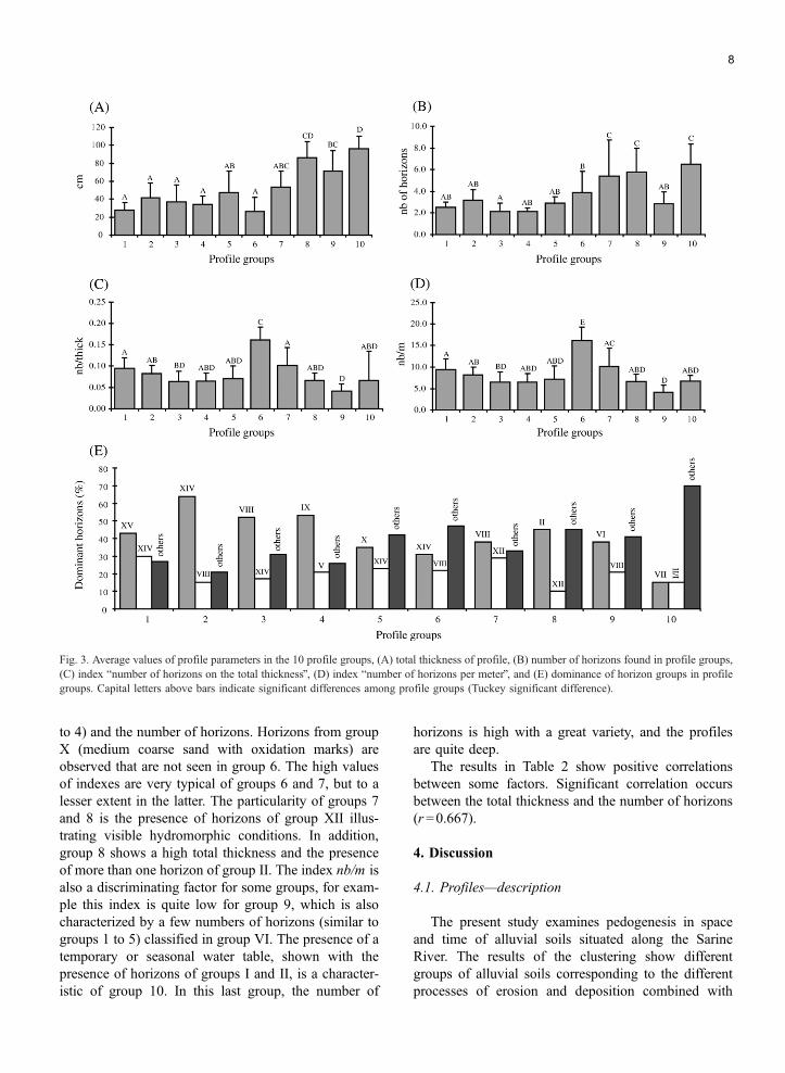
Fig. 3. Average values of profile parameters in the 10 profile groups, (A) total thickness of profile, (B) number of horizons found in profile groups,
(C) index bnumber of horizons on the total thicknessQ, (D) index bnumber of horizons per meterQ, and (E) dominance of horizon groups in profile
groups. Capital letters above bars indicate significant differences among profile groups (Tuckey significant difference).
8
to 4) and the number of horizons. Horizons from group
X (medium coarse sand with oxidation marks) are
observed that are not seen in group 6. The high values
of indexes are very typical of groups 6 and 7, but to a
lesser extent in the latter. The particularity of groups 7
and 8 is the presence of horizons of group XII illus-
trating visible hydromorphic conditions. In addition,
group 8 shows a high total thickness and the presence
of more than one horizon of group II. The index nb/m is
also a discriminating factor for some groups, for exam-
ple this index is quite low for group 9, which is also
characterized by a few numbers of horizons (similar to
groups 1 to 5) classified in group VI. The presence of a
temporary or seasonal water table, shown with the
presence of horizons of groups I and II, is a character-
istic of group 10. In this last group, the number of
horizons is high with a great variety, and the profiles
are quite deep.
The results in Table 2 show positive correlations
between some factors. Significant correlation occurs
between the total thickness and the number of horizons
(r=0.667).
4. Discussion
4.1. Profiles—description
The present study examines pedogenesis in space
and time of alluvial soils situated along the Sarine
River. The results of the clustering show different
groups of alluvial soils corresponding to the different
processes of erosion and deposition combined with
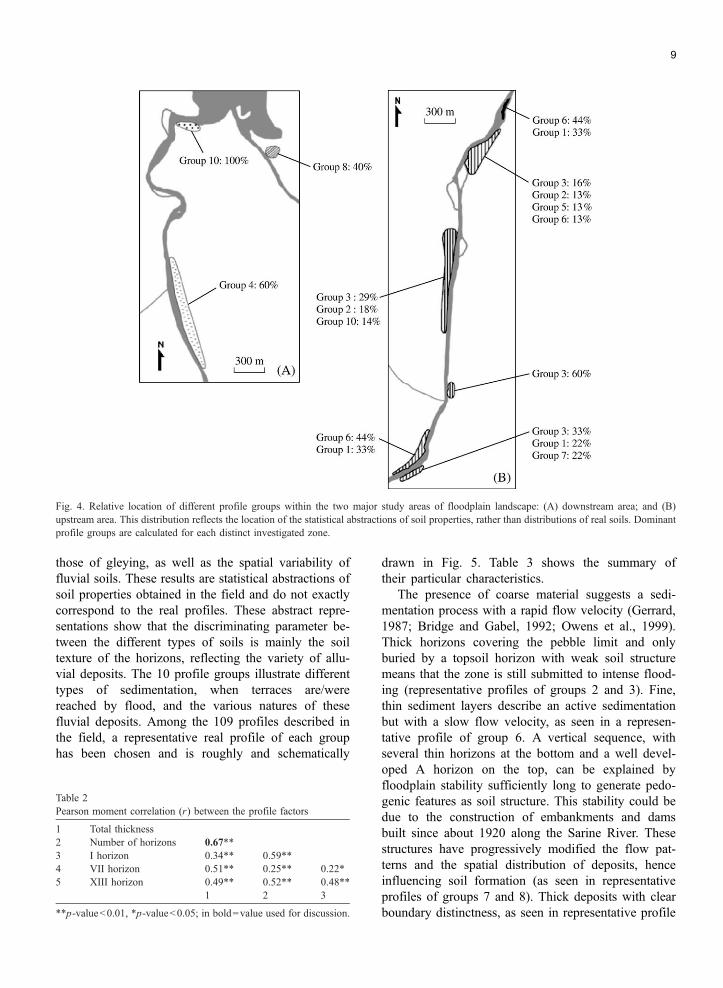
Fig. 4. Relative location of different profile groups within the two major study areas of floodplain landscape: (A) downstream area; and (B)
upstream area. This distribution reflects the location of the statistical abstractions of soil properties, rather than distributions of real soils. Dominant
profile groups are calculated for each distinct investigated zone.
9
those of gleying, as well as the spatial variability of
fluvial soils. These results are statistical abstractions of
soil properties obtained in the field and do not exactly
correspond to the real profiles. These abstract repre-
sentations show that the discriminating parameter be-
tween the different types of soils is mainly the soil
texture of the horizons, reflecting the variety of allu-
vial deposits. The 10 profile groups illustrate different
types of sedimentation, when terraces are/were
reached by flood, and the various natures of these
fluvial deposits. Among the 109 profiles described in
the field, a representative real profile of each group
has been chosen and is roughly and schematically
Table 2
Pearson moment correlation (r) between the profile factors
1 Total thickness
2 Number of horizons 0.67**
3 I horizon 0.34** 0.59**
4 VII horizon 0.51** 0.25** 0.22*
5 XIII horizon 0.49** 0.52** 0.48**
1 2 3
**p-valueb0.01, *p-valueb0.05; in bold=value used for discussion.
drawn in Fig. 5. Table 3 shows the summary of
their particular characteristics.
The presence of coarse material suggests a sedi-
mentation process with a rapid flow velocity (Gerrard,
1987; Bridge and Gabel, 1992; Owens et al., 1999).
Thick horizons covering the pebble limit and only
buried by a topsoil horizon with weak soil structure
means that the zone is still submitted to intense flood-
ing (representative profiles of groups 2 and 3). Fine,
thin sediment layers describe an active sedimentation
but with a slow flow velocity, as seen in a represen-
tative profile of group 6. A vertical sequence, with
several thin horizons at the bottom and a well devel-
oped A horizon on the top, can be explained by
floodplain stability sufficiently long to generate pedo-
genic features as soil structure. This stability could be
due to the construction of embankments and dams
built since about 1920 along the Sarine River. These
structures have progressively modified the flow pat-
terns and the spatial distribution of deposits, hence
influencing soil formation (as seen in representative
profiles of groups 7 and 8). Thick deposits with clear
boundary distinctness, as seen in representative profile
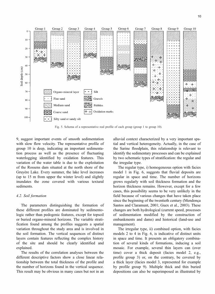
Fig. 5. Schema of a representative real profile of each group (group 1 to group 10).
10
9, suggest important events of smooth sedimentation
with slow flow velocity. The representative profile of
group 10 is deep, indicating an important sedimenta-
tion process as well as the presence of fluctuating
waterlogging identified by oxidation features. This
variation of the water table is due to the exploitation
of the Rossens dam situated at the north shore of the
Gruyere Lake. Every summer, the lake level increases
(up to 15 m from upper the winter level) and slightly
inundates the zone covered with various textural
sediments.
4.2. Soil formation
The parameters distinguishing the formation of
these different profiles are dominated by sedimento-
logic rather than pedogenic features, except for topsoil
or buried organo-mineral horizons. The variable strati-
fication found among the profiles suggests a spatial
variation throughout the study area and is involved in
the soil formation. The vertical sequences of distinct
layers contain features reflecting the complex history
of the site and should be clearly identified and
explained.
The results of the correlation analyses between the
different descriptive factors show a close linear rela-
tionship between the total thickness of the profile and
the number of horizons found in the vertical sequence.
This result may be obvious in many cases but not in an
alluvial context characterized by a very important spa-
tial and vertical heterogeneity. Actually, in the case of
the Sarine floodplain, this relationship is relevant to
identify the sedimentary processes and can be explained
by two schematic types of stratification: the regular and
the irregular type.
The regular type, i) homogeneous option with facies
model 1 in Fig. 6, suggests that fluvial deposits are
regular in space and time. The number of horizons
grows regularly with soil thickness formation and the
horizon thickness remains. However, except for a few
cases, this possibility seems to be very unlikely in the
field because of various changes that have taken place
since the beginning of the twentieth century (Mendonca
Santos and Claramunt, 2001; Guex et al., 2003). These
changes are both hydrological (current speed, processes
of sedimentation modified by the construction of
embankments and dams) and historical (land-use and
management).
The irregular type, ii) combined option, with facies
models 2 to 4 in Fig. 6, is indicative of distinct units
in space and time. It presents an obligatory combina-
tion of several kinds of formations, inducing a soil
mosaic. For example, several thin layers can (over
time) cover a thick deposit (facies model 2, e.g.,
profile group 3) or, on the contrary, be covered by
a thick layer (facies model 3, represented for example
by profile group 9). Multiple thick and thin buried
depositions can also be superimposed as illustrated by
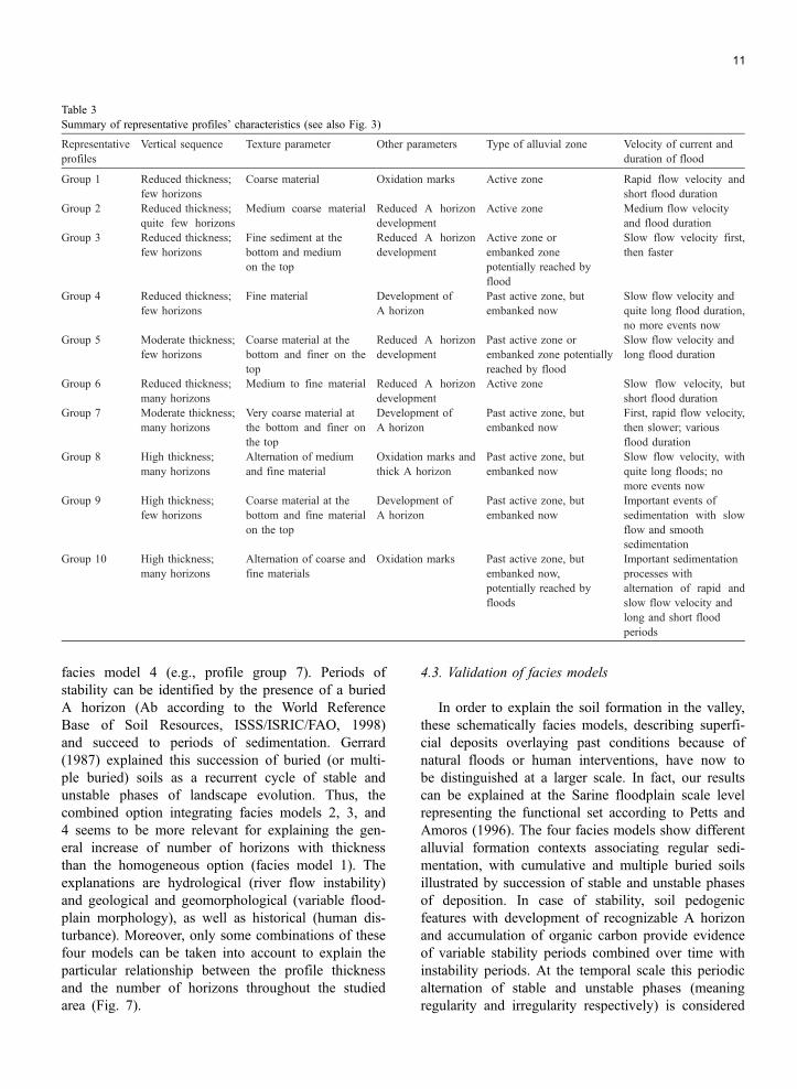
Table 3
Summary of representative profiles’ characteristics (see also Fig. 3)
Representative
profiles
Vertical sequence Texture parameter Other parameters Type of alluvial zone Velocity of current and
duration of flood
Group 1 Reduced thickness;
few horizons
Coarse material Oxidation marks Active zone Rapid flow velocity and
short flood duration
Group 2 Reduced thickness;
quite few horizons
Medium coarse material Reduced A horizon
development
Active zone Medium flow velocity
and flood duration
Group 3 Reduced thickness;
few horizons
Fine sediment at the
bottom and medium
on the top
Reduced A horizon
development
Active zone or
embanked zone
potentially reached by
flood
Slow flow velocity first,
then faster
Group 4 Reduced thickness;
few horizons
Fine material Development of
A horizon
Past active zone, but
embanked now
Slow flow velocity and
quite long flood duration,
no more events now
Group 5 Moderate thickness;
few horizons
Coarse material at the
bottom and finer on the
top
Reduced A horizon
development
Past active zone or
embanked zone potentially
reached by flood
Slow flow velocity and
long flood duration
Group 6 Reduced thickness;
many horizons
Medium to fine material Reduced A horizon
development
Active zone Slow flow velocity, but
short flood duration
Group 7 Moderate thickness;
many horizons
Very coarse material at
the bottom and finer on
the top
Development of
A horizon
Past active zone, but
embanked now
First, rapid flow velocity,
then slower; various
flood duration
Group 8 High thickness;
many horizons
Alternation of medium
and fine material
Oxidation marks and
thick A horizon
Past active zone, but
embanked now
Slow flow velocity, with
quite long floods; no
more events now
Group 9 High thickness;
few horizons
Coarse material at the
bottom and fine material
on the top
Development of
A horizon
Past active zone, but
embanked now
Important events of
sedimentation with slow
flow and smooth
sedimentation
Group 10 High thickness;
many horizons
Alternation of coarse and
fine materials
Oxidation marks Past active zone, but
embanked now,
potentially reached by
floods
Important sedimentation
processes with
alternation of rapid and
slow flow velocity and
long and short flood
periods
11
facies model 4 (e.g., profile group 7). Periods of
stability can be identified by the presence of a buried
A horizon (Ab according to the World Reference
Base of Soil Resources, ISSS/ISRIC/FAO, 1998)
and succeed to periods of sedimentation. Gerrard
(1987) explained this succession of buried (or multi-
ple buried) soils as a recurrent cycle of stable and
unstable phases of landscape evolution. Thus, the
combined option integrating facies models 2, 3, and
4 seems to be more relevant for explaining the gen-
eral increase of number of horizons with thickness
than the homogeneous option (facies model 1). The
explanations are hydrological (river flow instability)
and geological and geomorphological (variable flood-
plain morphology), as well as historical (human dis-
turbance). Moreover, only some combinations of these
four models can be taken into account to explain the
particular relationship between the profile thickness
and the number of horizons throughout the studied
area (Fig. 7).
4.3. Validation of facies models
In order to explain the soil formation in the valley,
these schematically facies models, describing superfi-
cial deposits overlaying past conditions because of
natural floods or human interventions, have now to
be distinguished at a larger scale. In fact, our results
can be explained at the Sarine floodplain scale level
representing the functional set according to Petts and
Amoros (1996). The four facies models show different
alluvial formation contexts associating regular sedi-
mentation, with cumulative and multiple buried soils
illustrated by succession of stable and unstable phases
of deposition. In case of stability, soil pedogenic
features with development of recognizable A horizon
and accumulation of organic carbon provide evidence
of variable stability periods combined over time with
instability periods. At the temporal scale this periodic
alternation of stable and unstable phases (meaning
regularity and irregularity respectively) is considered
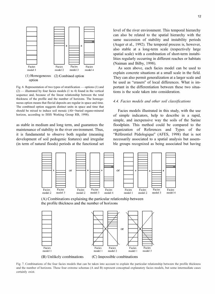
Fig. 6. Representation of two types of stratification — options (1) and
(2) — illustrated by four facies models (1 to 4) found in the vertical
sequence and, because of the linear relationship between the total
thickness of the profile and the number of horizons. The homoge-
neous option means that fluvial deposits are regular in space and time.
The combined option suggests distinct units in space and time that
should be mixed to induce soil mosaic (Ab=buried organo-mineral
horizon, according to ISSS Working Group RB, 1998).
12
as stable in medium and long term, and guarantees the
maintenance of stability in the river environment. Thus,
it is fundamental to observe both regular (meaning
development of soil pedogenic features) and irregular
(in term of natural floods) periods at the functional set
Fig. 7. Combinations of the four facies models that can be taken into accou
and the number of horizons. These four extreme schemas (A and B) represe
certainly exist.
level of the river environment. This temporal hierarchy
can also be related to the spatial hierarchy with the
same succession of stability and instability periods
(Auger et al., 1992). The temporal process is, however,
also stable at a long-term scale (respectively large
spatial scale) with a combination of short-term instabi-
lities regularly occurring in different reaches or habitats
(Naiman and Bilby, 1998).
As seen above, each facies model can be used to
explain concrete situations at a small scale in the field.
They can also permit generalization at a larger scale and
be used as berasersQ of local differences. What is im-
portant in the differentiation between these two situa-
tions is the scale taken into consideration.
4.4. Facies models and other soil classifications
Facies models illustrated in this study, with the use
of simple indicators, help to describe in a rapid,
simple, and inexpensive way the soils of the Sarine
floodplain. This method could be compared to the
organization of References and Types of the
bReferentiel PedologiqueQ (AFES, 1998) that is not
necessarily associated to a spatial analysis but assem-
ble groups recognized as being associated but having
nt to explain the particular relationship between the profile thickness
nt conceptual explanatory facies models, but some intermediate cases
13
ill-defined limits. Thus, it is not a new soil mapping
technique (using kriging and GIS methods like fuzzy
soil mapping) but a soil survey method that could help
to investigate rapidly the soils of an entire floodplain
valley. Nevertheless, it could be compared with the
fuzzy soil mapping as mentioned by Shi et al. (2004)
or the indicator kriging approach (Bierkens and Bur-
rough, 1993) that exclude the problems related with
the high cost (on money, labour, and time) and the
high subjectivity associated with the standard soil
surveys. These approaches, using mathematical equa-
tions, share some similarities with our facies models in
terms of soil properties and combinations. They can
be used to show the depth of different horizons or the
texture of A horizon (Shi et al., 2004). But if the
indicator kriging approach can be used for predicting
categorical soil data and producing maps with defined
boundaries, our facies models can interpret soil data at
different scale levels—in space and time—and relate
these to ancient landscape descriptions and floodplain
evolution.
5. Conclusions
The example of the Sarine River valley in the NWof
the Swiss Alps shows that the soil formation in alluvial
environment is highly heterogeneous and reveals dis-
tinctive sedimentologic and pedologic characteristics.
Frequent depositional disturbances from flooding, as
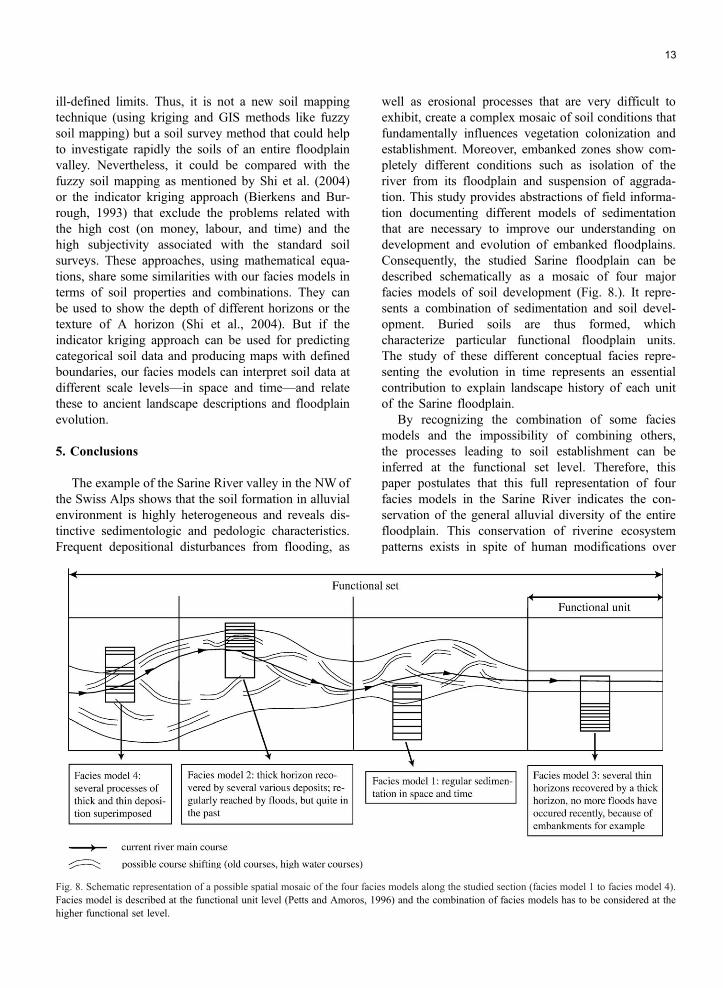
Fig. 8. Schematic representation of a possible spatial mosaic of the four fac
Facies model is described at the functional unit level (Petts and Amoros, 1
higher functional set level.
well as erosional processes that are very difficult to
exhibit, create a complex mosaic of soil conditions that
fundamentally influences vegetation colonization and
establishment. Moreover, embanked zones show com-
pletely different conditions such as isolation of the
river from its floodplain and suspension of aggrada-
tion. This study provides abstractions of field informa-
tion documenting different models of sedimentation
that are necessary to improve our understanding on
development and evolution of embanked floodplains.
Consequently, the studied Sarine floodplain can be
described schematically as a mosaic of four major
facies models of soil development (Fig. 8.). It repre-
sents a combination of sedimentation and soil devel-
opment. Buried soils are thus formed, which
characterize particular functional floodplain units.
The study of these different conceptual facies repre-
senting the evolution in time represents an essential
contribution to explain landscape history of each unit
of the Sarine floodplain.
By recognizing the combination of some facies
models and the impossibility of combining others,
the processes leading to soil establishment can be
inferred at the functional set level. Therefore, this
paper postulates that this full representation of four
facies models in the Sarine River indicates the con-
servation of the general alluvial diversity of the entire
floodplain. This conservation of riverine ecosystem
patterns exists in spite of human modifications over
ies models along the studied section (facies model 1 to facies model 4).
996) and the combination of facies models has to be considered at the

14
the last 150 yr and suggests a high potential for an
eventual revitalisation of embanked zones. However,
this occurrence of all alluvial facies models at the
functional set level does not prevent appearance of
bunbalancedQ zones at a smaller spatial scale level
where only one or two facies models remain. Thus,
the entire floodplain (functional set level), not only the
smaller scale functional alluvial unit, is the seemingly
obvious pertinent level needed to understand for the
long-term conservation of a complete alluvial system.
A real space–time balance should then exist between
the different facies models at a larger scale. This
spatial or temporal proportion between models also
depends on the damages that the system underwent.
Results documenting the different sedimentation mod-
els have then great significance for river management
and restoration activities in the alpine floodplain con-
text. For example, restoration management in a flood-
plain section — btrue and durableQ — should find the
balance between facies models by re-creating one
model or even more. Improved scientific understand-
ing of sedimentation and soil formation within the
embanked fluvial hydrosystem will enhance effective
management by finding equilibrium inside all types of
floodplain ecosystems.
Acknowledgements
This research is supported by the Swiss National
Science Foundation (PNR 48: Floodplains of the Al-
pine Arc, between security and biodiversity, project no.
4048-064357); the Swiss Agency for the Environments,
Forests and Landscape; and the Swiss Federal Office
for Water and Geology. The authors would like to thank
Anne Gerber and Nicolas Kueffer who greatly im-
proved the manuscript.
References
AFES, 1998. A Sound Reference Base for Soils, The TReferentiel
Pedologiquer. INRA Editions, Paris.
Auger, P., Baudry, J., Fournier, F., 1992. Hierarchies et Echelles en
Ecologie. Naturalia Publications, Turriers.
Autin, W.J., Aslan, A., 2001. Alluvial pedogenesis in Pleistocene and
Holocene Mississippi River deposits: effects of relative sea-level
change. Geological Society of America Bulletin 113, 1456–1466.
Bierkens, M.F.P., Burrough, P.A., 1993. The indicator approach
to categorical soil data: I. Theory. Journal of Soil Science 44,
361–368.
Bragato, G., 2004. Fuzzy continuous classification and spatial inter-
polation in conventional soil survey for soil mapping of the lower
Piave plain. Geoderma 118, 1–16.
Bridge, J.S., Gabel, S.L., 1992. Flow and sediment dynamics in a low
sinuosity, braided river—Calamus River, Nebraska Sandhills.
Sedimentology 39, 125–142.
Bronger, A., Catt, J.A., 1998. Summary outline and recommendations
on paleopedological issues. Quaternary International 51/52, 5–6.
Bureau, F., Guenat, C., Thomas, C., Vedy, J.-C., 1995. Human
impacts on alluvial flood plain stretches: effects on soils and
soil vegetation relations. Arch. Hydrobiol. Suppl. 101 Large
Rivers 9, 147-161.
Cosandey, A.C., Guenat, C., Bouzelboudjen, M., Maitre, W., Bovier,
R., 2003. The modelling of soil-process functional units based on
three-dimensional soil horizon cartography, with an example of
denitrification in a riparian zone. Geoderma 112, 111–129.
Daniels, J.M., 2003. Floodplain aggradation and pedogenesis in a
semiarid environment. Geomorphology 56, 225–242.
Earl, R., Taylor, J.C., Wood, G.A., Bradley, I., James, I.T., Waine,
T., Welsh, J.P., Godwin, R.J., Knight, S.M., 2003. Soil factors
and their influence on within-field crop variability: part 1.
Field observation of soil variation. Biosystems Engineering 84,
425–440.
Fierz, M., Gobat, J.-M., Guenat, C., 1995. Quantification et caracteri-
sation de la matiere organique de sols alluviaux au cours de
l’evolution de la vegetation. Annales des sciences forestieres 52,
547–559.
Gerrard, J., 1987. Alluvial Soils. Hutchinson Ross, New York.
Gerrard, J., 2000. Fundamentals of Soils. Routledge, New York.
Gobat, J.-M., Aragno, M., Matthey, W., 2004. The Living Soil,
Fundamentals of Soil Science and Soil Biology. Science Publi-
shers, Enfield.
Guex, D., Weber, G., Musy, A., Gobat, J.-M., 2003. Evolution of a
Swiss alpine floodplain over the last 150 years: hydrological and
pedological considerations. The Warsaw International Conference
of Ecoflood, Towards Natural Flood Reduction Strategies. Eco-
flood Network, Poland.
Ihaka, R., Gentleman, R., 1996. R: a language for data analysis and
graphics. Journal of Computational and Graphical Statistics 5,
299–314.
ISSS/ISRIC/FAO, 1998. World reference base for soil resources.
World Soil Rec. Rep, vol. 84. FAO, Rome.
Kraus, J.J, Brown, T.M., 1988. Pedofacies analysis; a new approach
to reconstructing ancient fluvial sequences. In: Reinhardt, J.,
Sigleo, W.R. (Eds.), Paleosols and Weathering Through Geologic
Time: Principles and Applications, The Geological Society of
America, Special Paper, vol. 216. The Geological Society of
America, Boulder, CO, pp. 143–152.
Legendre, P., Legendre, L., 2000. Numerical Ecology. Elsevier,
Amsterdam.
McAuliffe, J.R., 1994. Landscape evolution, soil formation, and
ecological patterns and processes in Sonoran Desert Bajadas.
Ecological Monographs 64, 111–148.
Mendonca Santos, M.L., Claramunt, C., 2001. An integrated land-
scape and local analysis of land cover evolution in alluvial zone.
Computers, Environment and Urban Systems 25, 557–577.
Mendonca Santos, M.L., Guenat, C., Thevoz, C., Bureau, F., Vedy,
J.-C., 1997. Impacts of embanking on the soil–vegetation rela-
tionships in a floodplain ecosystem of a pre-alpine river. Global
Ecology and Biogeography Letters 6, 339–348.
Mendonca Santos, M.L., Guenat, C., Bouzelboudjen, M., Golay, F.,
2000. Three-dimensional GIS cartography applied to the study of
the spatial variation of soil horizons in a Swiss floodplain. Geo-
derma 97, 351–366.
Naiman, R.J., Bilby, R.E., 1998. River Ecology and Management.
Springer, New York.
Owens, P.N., Walling, D.E., Leeks, G.J.L., 1999. Use of floodplain
sediment cores to investigate recent historical changes in overbank

,
15
sedimentation rates and sediment sources in the catchment of the
River Ouse, Yorkshire, UK. Catena 36, 21–47.
Paton, T.R., Humphreys, G.S., Mitchell, P.B., 1995. Soils—A New
Global View. UCL Press, London.
Petts, G.E., Amoros, C., 1996. Fluvial Hydrosystems. Chapman and
Hall, London.
Shi, X., Zhu, A.-X., Burt, J.E., Qi, F., Simonson, D., 2004. A case-
based reasoning approach to fuzzy soil mapping. Soil Science
Society of America Journal 68, 885–894.
Thoms, M.C., 2003. Floodplain–river ecosystems: lateral connections
and the implications of human interference. Geomorphology 56
335–349.
Top Related