


Languages
Pages
Legal


Hypoxia in Narragansett BayWorkshop Oct 2006
“Modeling”In the Narragansett Bay
CHRP Project
Dan Codiga, Jim Kremer, Mark Brush, Chris Kincaid, Deanna
Bergondo

Does the word “Model” have meaning?
• Hydrodynamic
• Ecological
• Research vs Applied
• Prognostic vs Diagnostic
• Heuristic, Theoretical, Conceptual, Empirical, Statistical, Probabilistic, Numerical, Analytic
• Idealized/Process-Oriented vs Realistic
• Kinematic vs Dynamic
• Forecast vs hindcast


CHRP Program Goals (selected excerpts from RFP)
• Predictive/modeling tools for decision makers
• Models that predict susceptibility to hypoxia
• Better understanding and parameterizations
• Transferability of results across systems
• Data to calibrate and verify models
Following two presentations

Our approaches• Hybrid Ecological-Hydrodynamic Modeling
– Ecological model: simple• Few processes, few parameters• Parameters that can be constrained by measurements• Few spatial domains (~20), as appropriate to measurements available• Net exchanges between spatial domains: from hydrodynamic model
– Hydrodynamic model: full physics and forcing of ROMS• realistic configuration; forced by observed winds, rivers, tides, surface fluxes• Applied across entire Bay, and beyond, at high resolution• Passive tracers used to determine net exchanges between larger domains of
ecological model
• Empirical-Statistical Modeling– Input-output relations, emphasis on empirical fit more than mechanisms– Development of indices for stratification, hypoxia susceptibility– Learn from hindcasts, ultimately apply toward forecasting

Heuristic models in research: iterative failure = learning
ConceptualModel
Runs that fall short
Processes
Formulations
Parameter values

But for management models:• Heuristic goal less impt
• Accurate even if not precise
• Well constrained coefs• Simple (?) (at least understandable)
_____________________________ ≠ Research models

A paradox --
“Realism” = many parameters weakly constrained limited data to corroborate
i.e. “Over-parameterized” (many ways to get similar results)
:. Accuracy is
unknown. (often unknowable)

An alternative approach? 4 state variables, 5 processes
N P
N
Land-use
Atmosphericdeposition
N P
Productivity
Temp, Light,Boundary Conditions
Chl, N, P, Salinity
Phytoplankton
Sedimentorganics
.
.
Physics
Surface layer
- - - - - - - - -
Deep layer
- - - - - - - - -
Bottom sediment
O2
Flux tobottom
Photic zoneheterotrophy
Benthicheterotrophy Denitri-
fication
O2 coupledstoichiometrically
Processes of the model (excluding macroalgae...)
mixing flushing

Corroboration:“Strength in numbers”
Shallow test sites (MA, RI,
CT)

Long Island Sound -- Hypoxia
August 20
Deep test sites (MA, RI, CT, VA, MD)
Chesapeake Bay
Narragansett Bay
Long Island Sound

Initial Conditions
Forcing Conditions
Output
EquationsMomentum balance x & y directions:u + vu – fv = + Fu + Du t xv + vv + fu = + Fv + Dv t yPotential temperature and salinity :T + vT = FT + DT
t S + v S = FS + DS
t The equation of state:= (T, S, P) Vertical momentum: = - gz o
Continuity equation:u + v + w = 0x y z
Hydrodynamic Model
ROMS Model
Regional Ocean Modeling System

Grid Resolution: 100 mGrid Size: 1024 x 512Vertical Layers: 20River Flow: USGSWinds: NCDCTidal Forcing: ADCIRC
Open Boundary
Hydrodynamic Model

This project: Mid-Bay focus
Extent of counterMt. Hope Bay circulation/exchange/mixing study. ADCP, tide gauges (Deleo, 2001)
Bay-RIS exchange study (98-02)
Narragansett Bay Commission: Providence & Seekonk Rivers
Summer, 07: 4 month deployment (Outflow pathways)

This project: Mid-Bay focus
Extent of counterMt. Hope Bay circulation/exchange/mixing study. ADCP, tide gauges (Deleo, 2001)
Bay-RIS exchange study (98-02)
Narragansett Bay Commission: Providence & Seekonk Rivers
Summer, 08: Deep return flow processes

Model-Data Comparison
Salinity - Phillipsdale
Sal
inity
(pp
t)
Time (days)
Model
Data

Model-Data ComparisonShallows: North-South Component
-0.25
-0.15
-0.05
0.05
0.15
10 15 20
Time
Model Velocity
(m/s)
-250
-150
-50
50
150
Observed Velocity
(mm/s)
Bottom-model
Bottom
Channel: North-South Component
-0.25
-0.15
-0.05
0.05
0.15
0.25
10 15 20
Time (days)
Model Velocity
(m/s)
-250
-150
-50
50
150
250
Obsevered Velocity (m/s)
Bottom-model
Bottom
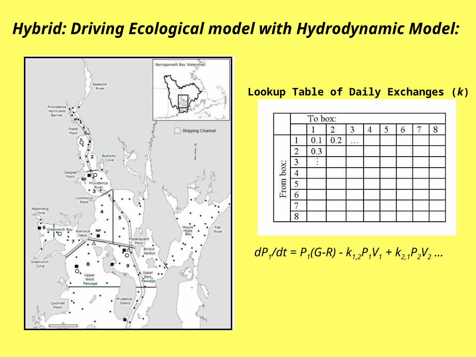
dP1/dt = P1(G-R) - k1,2P1V1 + k2,1P2V2 ...
Hybrid: Driving Ecological model with Hydrodynamic Model:
Lookup Table of Daily Exchanges (k)
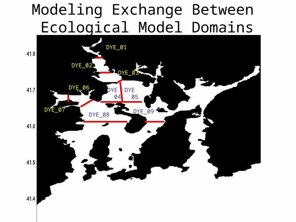
DYE_08
DYE_02DYE_03
DYE 05
DYE_01
DYE_09DYE_07
DYE_06 DYE 04
Modeling Exchange Between Ecological Model Domains

Passive Tracer Experiment

Passive Tracer Experiment

Passive Tracer Experiment

Long-term Aims:Hybrid Ecological-Physical Model
• Increased spatial resolution of ecology: approach TMDL applicability
• Scenario evaluation– Nutrient load changes– Climatic changes
• Alternative to mechanistic coupled hydrodynamic/ecological modeling

Empirical/Statistical ModelingOverall Goals
• Data-oriented—complements Hybrid– less mechanistic• Synthesize DO variability
– Spatial (Large-scale CTD; towed body)
– Temporal (Fixed-site buoys)
• Develop indices– Stratification
– Hypoxia vulnerability
• First: Hindcasts to understand relationship between forcing (physical and biological) and DO responses
• Long-term: Predictive capability for forecasting and scenario evaluation

• Candidate predictors for DO– Biological
• Chlorophyll• Temperature & solar input• Nutrient inputs (Rivers, WWTF, Estuarine
exchange) • Others
– Physical • River runoff, WWTF water transports• Tidal range cubed (energy available for mixing)• Windspeed cubed (energy available for mixing)• Others (Wind direction; Precip; Surface heat flux)


Strategy: start simple & develop method
• Start with Bullock Reach timeseries– 5 yrs at fixed single point (no spatial information)
• Investigate stratification (not DO-- yet)– Target variable: strat = [sigt(deep) – sigt(shallow)]– Include 3 candidate predictor variables:
• River runoff (sum over 5 rivers)
• Tidal range cubed (energy available for mixing)
• Windspeed cubed (energy available for mixing)

2001
Visually apparent features
• Stratification reacts to ‘events’ in each of:– River inputs– Winds– Tidal stage
• Stratification ‘events’ appear to be– Triggered irregularly by each process– Lagged by varying amounts from each process

Low-pass and subsample to 12 hrs…Compare techniques
• Multiple Linear Regression (MLR)– No lags– Optimal lags – determined individually
• Static Neural Network– No lags– Lags from MLR analysis
• [coming soon] Dynamic Neural Network– Varying lags– Multiple interacting inputs

Multiple Linear Regression
No lagsr2=0.42 (River alone: 0.36)
Observed Model
MLR with lags River 2 days Wind 1 day Tide 3.5 days
r2=0.51 (River alone: 0.48)
Stratificationt [kg m-3]
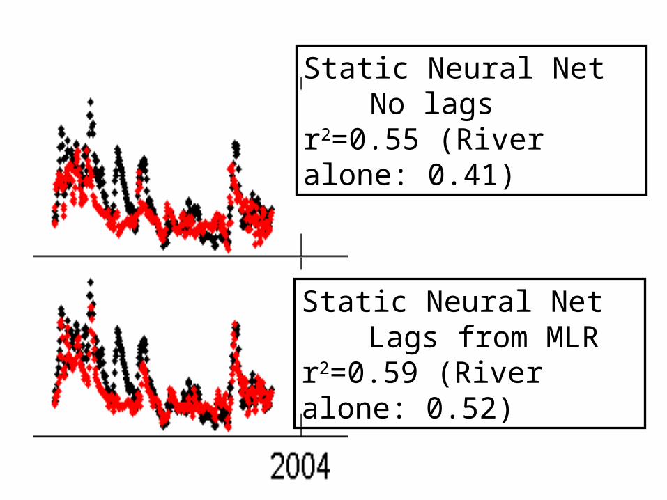
Static Neural NetNo lags
r2=0.55 (River alone: 0.41)
Static Neural NetLags from MLR
r2=0.59 (River alone: 0.52)

Advantages/Disadvantagesof Neural Networks
• Advantages– Nonlinear, can achieve better accuracy– Excels with multiple interacting predictors; – Dynamic NN: input delays capture lags
• Varying lags from multiple interacting inputs
– Transferable; conveniently applied to other/new data– Easy to use (surprise!!)
• Main disadvantage– opaque “black-box” can be difficult to interpret;
ameliorated by: complementary linear analysis, sensitivity studies, isolating/combining predictors

Next steps
• Stratification– Consider additional predictors:
• Surface heat flux; precipitation; WWTF volume flux
– Different sites (North Prudence, etc)– Treat spatially-averaged regions
• Apply similar approach to DO– Finish gathering forcing function data
• Chl; solar inputs; WWTF nutrients
– Corroborate Hybrid Ecological-Hydrodynamic Model
Top Related