


Languages
Pages
Legal

Hydraulic TransporT of sand/sHell MixTures in relaTion WiTH THe criTical VelociTy
sape a. MiedeMa and roBerT c. raMsdell
ABSTRACT
When pumping shells through a pipeline one
must consider that shells are not spherical,
but more disc-shaped. When shells settle they
will settle like leaves where the biggest cross
section is exposed to the drag. But they will
settle in the same orientation, flat on the
sediment, so the sides of the shells are
exposed to the horizontal flow in the pipeline.
Since the side cross section is much smaller
than the horizontal cross section, a much
higher velocity is required to make them
erode and go back into suspension.
The settling velocity is much smaller because
of the large area of the cross section. Even
when the slurry velocity exceeds the settling
velocity, some shells will reach the bottom of
the pipe owing to the combination of settling
velocity and turbulence. Once these shells are
on top of the sediment they are hard to
remove by erosion, because they lay flat on
the surface and only a small cross section is
exposed to the flow compared with the
weight of the shell.
So although their settling velocity is much
lower than equivalent sand particles, the
erosion velocity is much higher. On a shell-
covered beach, shells are always visible on top
of the sand. In fact, these shells are shielding
the sand from erosion. Bigger shells will also
shield the smaller pieces, because smaller
pieces settle faster. Shells settle more slowly
than sand grains, so they will be on top of
the bed (if there is a bed) just as on the beach.
These shells are hard to erode, in fact, they
protect the bed from being eroded, even if
the line speed is increased. The combination
of high erosion velocity and the shells
“protecting” the bed means that even a small
amount of shells can lead to relatively thick
bed in the pipeline. But there will always be
a velocity above the bed that will make the
shells erode.
This article describes the settling and erosion
process of shells and the consequences of
this on the critical velocity when pumping
a sand/shell mixture through a pipeline.
A mathematical model of the processes
involved will be presented.
INTRODUCTION
When pumping shells through a pipeline one
must consider that shells are not spherical,
but more disc shaped. When shells settle they
will settle like leaves where the biggest cross
section is exposed to the drag. But when they
settle, they will settle in the same orientation,
flat on the sediment, so the side of the shells
is exposed to the horizontal flow in the
pipeline. Since the side cross section is much
smaller than the horizontal cross section,
a much higher velocity is required to make
them erode and go back into suspension.
The settling velocity is much smaller because
of the large area of the cross section. Normally pipeline resistance is calculated based
on the settling velocity, where the resistance is
proportional to the settling velocity of the
grains. The critical velocity is also proportional
with the settling velocity. Since shells have a
much lower settling velocity than sand grains
with the same weight and much lower than
sand grains with the same sieve diameter,
one would expect a much lower resistance
and a much lower critical velocity, matching
the lower settling velocity.
This is only partly true. As long as the shells
are in suspension, on average they want to
stay in suspension because of the low settling
Above: A shell-covered beach provides protection,
shielding the sand from erosion. But when pumping
shells through a pipeline the line speed must be
considered. If line speed decreases so much that the
erosion flux is less than the sedimentation flux, not all
the particles will be eroded, resulting in a bed forming
at the bottom of the pipe as it does on the beach.
18 Terra et Aqua | Number 122 | March 2011

Hydraulic Transport of Sand /Shell Mixtures in Relation with the Critical Velocity 19
velocity. But settling and erosion are
stochastic processes because of the turbulent
character of the flow in the pipeline. Since we
operate at Reynolds numbers above 1 million,
the flow is always turbulent, meaning that
eddies and vortices occur stochastically
making the particles in the flow move up and
down, resulting in some particles hitting the
bottom of the pipe. Normally these particles
will be picked up in the flow because of
erosion, so there exists equilibrium between
sedimentation and erosion, resulting in not
having a bed at the bottom of the pipeline.
In fact the capacity of the flow to erode is
bigger than the sedimentation. If the line
speed decreases, the shear velocity at the
bottom of the pipe also decreases and less
particles will be eroded, so the erosion
capacity is decreasing. This does not matter,
because as long as the erosion capacity is
bigger than the sedimentation, there will not
be sediment at the bottom of the pipeline.
As soon as the line speed decreases so much
that the erosion capacity (erosion flux) is
smaller than the sedimentation flux, not all
the particles will be eroded, resulting in a bed
to be formed at the bottom of the pipe.
Having a bed at the bottom of the pipe also
means that the cross section of the pipe
decreases and the actual flow velocity above
the bed increases. This will result in a new
equilibrium between sedimentation flux and
erosion flux for each bed height.
From the moment there is a bed, decreasing
the flow will result in an almost constant flow
velocity above the bed, resulting in equilibrium
between erosion and sedimentation.
This equilibrium however is sensitive for
changes in the line speed and in the mixture
density. Increasing the line speed will reduce
the bed height; a decrease will increase the
bed height. Having a small bed does not really
matter, but a thick bed makes the system
vulnerable for plugging the pipeline.
The critical velocity in most models is chosen in
such a way that a thin bed is allowed. As said
before, some shells will always will reach the
bottom of the pipe owing to the combination
of settling velocity and turbulence. Once these
shells are on top of the sediment they are hard
to remove by erosion, because they lay flat on
the surface and have a small cross section that
is exposed to the flow compared with the
weight of the shell. So although their settling
velocity is much lower than equivalent sand
particles, the erosion velocity is much higher.
Looking at a beach in an area with many
shells, there are always shells visible on top of
the sand, covering the sand. In fact the shells
are shielding the sand from erosion, because
they are hard to erode. The bigger shells will
also shield the smaller pieces, because the
smaller pieces settle faster. Compare this with
leaves falling from a tree, the bigger leaves,
although heavier, will fall slower, because they
are exposed to higher drag. The same process
will happen in the pipeline. Shells settle more
slowly than sand grains, so they will be on top
of the bed (if there is a bed), just as on the
beach. Since they are hard to erode, in fact, they
protect the bed from being eroded, even
if the line speed is increased. But there will
always be velocities above the bed that will
make the shells erode. Now the question is
how to quantify this behaviour in order to
get control over it.
One must distinguish between sedimentation
and erosion. First of all assume shells are disc
shaped with a diameter d and a thickness of
a • d and let’s take a = 0.1 this gives a cross
section for the terminal settling velocity of
π / 4 • d2, a volume of π / 40 • d3, and a cross
section for erosion of d2 / 10. Two processes
have to be analysed to determine the effect of
shells on the critical velocity: the sedimentation
process and the erosion process.
THe sediMenTaTion processThe settling velocity of grains depends on the
grain size, shape and specific density. It also
depends on the density and the viscosity of
the fluid the grains are settling in and upon
whether the settling process is laminar or
turbulent. Discrete particles do not change
their size, shape or weight during the settling
process (and thus do not form aggregates).
A discrete particle in a fluid will settle under
the influence of gravity. The particle will
accelerate until the frictional drag force of
the fluid equals the value of the gravitational
force, after which the vertical (settling)
velocity of the particle will be constant.
In general, the settling velocity vs can be
determined with the following equation:
vg d
Cs
q w
w d=
⋅ ⋅ − ⋅ ⋅
⋅ ⋅
4
3
( )ρ ρ ψ
ρ [1]
The settling velocity is thus dependent on: the
density of the particle and fluid, diameter (size)
and shape (shape factor ψ) of the particle, and
flow pattern around the particle. The Reynolds
number of the settling process determines
whether the flow pattern around the particle
is laminar or turbulent. The Reynolds number
can be determined by:
Figure 1. Drag coefficient as a function of the particle shape (Wu and Wang, 2006).
The drag coefficient for different shape factors
CD
Re
102
101
100
10-1
100 101 102 103 104 105 106
Sf=1.0 Sf=0.80-0.99
Sf=1.0 Sf=0.9 Sf=0.7
Sf=0.6-0.79
Sf=0.5
Sf=0.4-0.59
Sf=0.3
Sf=0.20-0.39
Strokes
20 Terra et Aqua | Number 122 | March 2011
Repsv d
=⋅ν [2]
The viscosity of the water is temperature
dependent. If a temperature of 10° is used as
a reference, then the viscosity increases by
27% at 0° and it decreases by 30% at 20°
centigrade. Since the viscosity influences
the Reynolds number, the settling velocity
for laminar settling is also influenced by
the viscosity. For turbulent settling the drag
coefficient does not depend on the Reynolds
number, so this settling process is not
influenced by the viscosity.
The drag coefficientThe drag coefficient C
d depends upon the
Reynolds number according to Turton and
Levenspiel (1986), which is a 5 parameter
fit function to the data:
dCp
pp
= ⋅ + ⋅ ++ ⋅ −
241 0 173
0 413
1 163000 657
1Re( . Re )
.
Re.
.009 [3]
It must be noted that in general the drag
coefficients are determined based on the
terminal settling velocity of the particles.
Wu and Wang (2006) recently gave an over-
view of drag coefficients and terminal settling
velocities for different particle Corey shape
factors. The result of their research is reflected
in Figure 1. Figure 1 shows the drag coefficients
as a function of the Reynolds number and as a
function of the Corey shape factor.
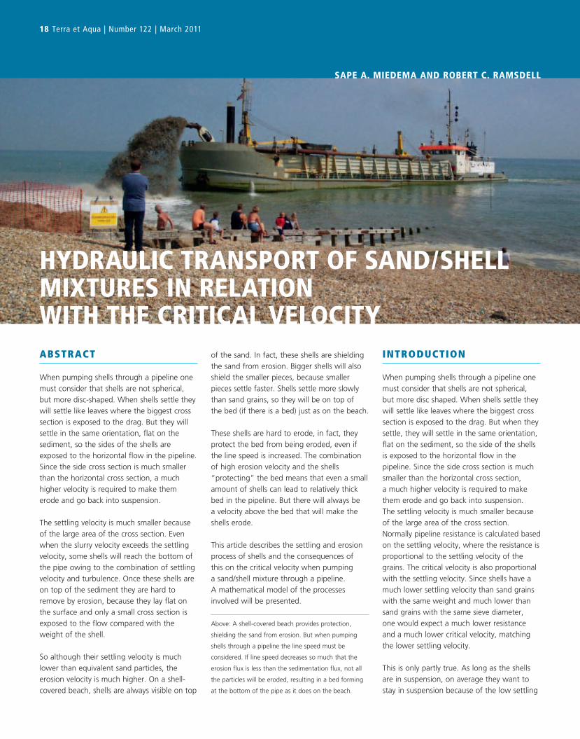
For shells settling the Corey shape factor is
very small, like 0.1, resulting in high drag
coefficients. According to Figure 2 the drag
coefficient should be like:
Hindered settlingThe above equations calculate the settling
velocities for individual grains. The grain moves
downwards and the same volume of water
has to move upwards. In a mixture, this means
that when many grains are settling, an
average upwards velocity of the water exists.
This results in a decrease of the settling
velocity, which is often referred to as hindered
settling. However, at very low concentrations
the settling velocity will increase because the
grains settle in each other’s shadow.
Richardson and Zaki (1954) determined an
equation to calculate the influence of hindered
settling for volume concentrations Cv between
0.05 and 0.65. Theoretically, the validity of the
Richardson and Zaki equation is limited by the
maximum solids concentration that permits
solids particle settling in a particulate cloud.
This maximum concentration corresponds with
the concentration in an incipient fluidised bed
(Cv of about 0.57). Practically, the equation
was experimentally verified for concentrations
not far above 0.30. The exponent in this
equation is dependent on the Reynolds
number. The general equation yields:
c
sv
vv
C= −( )β1 [7]
The following values for β should be used
(using the following definition does give a
continuous curve):
Rep<0.1 β=4.65
Rep>0.1 and Re
p<1.0 β=4.35 . Re
p-0.03
Rep>1.0 and Re
p<400 β=4.45 . Re
p-0.1
Rep>400 β=2.39
[8]
Other researchers found the same trend with
sometimes different values for the power β,
as shown in Figure 4.
ErosionIn Miedema (2010), a model for the
entrainment of particles as a result of fluid
(or air) flow over a bed of particles has been
developed. The model distinguishes sliding,
rolling and lifting as the mechanisms of
entrainment. Sliding is a mechanism that
occurs when many particles are starting to
move and it is based on the global soil
mechanical parameter of internal friction.
Both rolling and lifting are mechanisms of
C CDp
Dp
= + = +32
236
3Re Re
up to [4]
For shells lying flat on the bed, the drag
coefficient will be similar to the drag
coefficient of a streamlined half body (0.09),
which is much smaller than the drag
coefficient for settling (3).
So there is a large asymmetry between the
settling process and the erosion process of
shells, while for more or less spherical sand
particles the drag coefficient is considered to
be the same in each direction.
Terminal settling velocity equations from literatureThe shape factor was introduced into
equation (1) by multiplying the mass of a sand
particle with a shape factor ψ. For normal
sands this shape factor has a value of 0.7.
Zanke (1977) has derived an equation for
the transitional region (in m and m/sec):
vs =⋅⋅ +
⋅ ⋅
⋅−
101
1001
3
2
ννd
R g dd
[5]
With the relative density Rd defined as:
Rd =−ρ ρ
ρq w
w [6]
Figure 3 shows the settling velocity as a
function of the particle diameter for the
Stokes, Budryck, Rittinger and Zanke
equations. Instead of using the shape factor in
equation (1), it is better to use the actual drag
coefficient according to equation (4) giving
the shape factor a value of 1.
Sphere
Half Sphere
Cone
Cube
AngledCube
LongCylinder
ShortCylinder
StreamlinedBody
StreamlinedHalf-Body
0.47
0.42
0.50
1.05
0.80
Shape
Measured Drag Coefficients
0.82
1.15
0.04
0.09
DragCoefficient
Figure 2. Some drag coefficients (source Wikipedia).

Hydraulic Transport of Sand /Shell Mixtures in Relation with the Critical Velocity 21
individual particles and are based on local
parameters such as the pivot angle and the
exposure and protrusion rate. Equations (9),
(10) and (12) give the Shields parameter for
these 3 mechanisms.
Sliding
θαsliding
d
sliding
Drag D D
u
R g d f C=
⋅ ⋅= ⋅ ⋅
⋅ ⋅ +*2
2 2
43
1
l sliding L Lf C⋅ ⋅
µ
µ [9]
Rolling
θαrolling
d
rolling
Drag D D
u
R g d f C=
⋅ ⋅= ⋅ ⋅
⋅ ⋅ +*2
2 2
43
1l rolling L Lf C⋅ ⋅
µ
µ [10]
With the effective rolling friction coefficient
μrolling
:
ψ φψ φrollingRoll
L ever D Roll
=+
+ +−
sin( )
cos( )µ
l [11]
Lifting
θαlift ing
d L L
u
R g d C f=
⋅ ⋅=
⋅ ⋅*2
2
43
1
[12]
Non-uniform particle distributionsIn the model for uniform particle distributions,
the roughness ks was chosen equal to the
particle diameter d, but in the case of non-
uniform particle distributions, the particle
diameter d is a factor d+ times the roughness
ks, according to:
ddks
+ = [13]
The roughness ks should be chosen equal to
some characteristic diameter related to the
non-uniform particle distribution, for example
the d50
.
Laminar regionFor the laminar region (the viscous sub layer)
the velocity profile of Reichardt (1951) is
chosen. This velocity profile gives a smooth
transition going from the viscous sub layer
to the smooth turbulent layer.
uu y
u
ytop
top top++
= =+ ⋅
−+
⋅( ) ln( ) ln( / ) ln( )
*
1 1 91
κ
κκ
κ−− −
− +− ⋅
+
+
ey
e
ytop y
top
top11 6 0 33
11 6. .
.≈ +y top
uu y
u
ytop
top top++
= =+ ⋅
−+
⋅( ) ln( ) ln( / ) ln( )
*
1 1 91
κ
κκ
κ−− −
− +− ⋅
+
+
ey
e
ytop y
top
top11 6 0 33
11 6. .
.≈ +y top
[14]
For small values of the boundary Reynolds
number and thus the height of a particle,
SAPE A. MIEDEMA
obtained his MSc in Mechanical
Engineering with honours at the Delft
University of Technology (DUT) in 1983
and his PhD in 1987. From 1987 to the
present he has been at DUT, as assistant,
then associate, professor at the Chair of
Dredging Technology, then as a member of
the management board of Mechanical
Engineering and Marine Technology. From
1996 to 2001 he was appointed
educational director of Mechanical
Engineering and Marine Technology at
DUT, whilst remaining associate professor
of Dredging Engineering. In 2005, in
addition, he was appointed educational
director of the MSc programme of Offshore
Engineering.
ROBERT C. RAMSDELL
graduated with a BA in Mathematics from
the University Of California at Berkeley In
1986. He joined Great Lakes Dredge &
Dock Company, Oakbrook, Illinois in 1989
as a Field Engineer/Project Engineer/
Superintendent. In 1997 he became a
Production Engineer\Senior Production
Engineer. He is presently Production
Engineering Manager in the Administrative
Division of GLDD.
Figure 3. The settling velocity of individual particles.
Figure 4. The hindered
settling power according
to several researchers.
Settling velocity of real sand particles
Grainsize in mm
Sett
ling
vel
oci
ty in
mm
/sec
Stokes Budryck Rittinger Zanke
1000
100
10
1
0.10.01 0.1 1 10
Hindered settling power
Rep (-)
Bet
a (-
)
Rowe Wallis Garside Di Felice Richardson
7.00
6.00
5.00
4.00
3.00
2.00
0.001 0.01 0.1 1 10 100 1000 10000

22 Terra et Aqua | Number 122 | March 2011
the velocity profile can be made linear to:
u y d E d E ktop top s+ + + + += = ⋅ ⋅ = ⋅ ⋅Re* [15]
Adding the effective turbulent velocity to the
time averaged velocity, gives for the velocity
function aLam
:
αLam top eff topy u y= ++ + +( ) [16]
Turbulent regionParticles that extend much higher into the
flow will be subject to the turbulent velocity
profile. This turbulent velocity profile can be
the result of either a smooth boundary or a
rough boundary. Normally it is assumed that
for boundary Reynolds numbers less than 5
a smooth boundary exists, while for boundary
Reynolds numbers larger than 70 a rough
boundary exists. In between in the transition
zone the probability of having a smooth
boundary is:
P e eks
= =− ⋅ − ⋅
+0 95
11 60 95
11 6.
Re
..
.*
[17]
This probability is not influenced by the
diameter of individual particles, only by the
roughness ks which is determined by the
non-uniform particle distribution as a whole.
This gives for the velocity function aTurb
:
ακ δ κTurb
top
v
yP= ⋅ ⋅ + ⋅ + ⋅
+
+1
95 11
ln ln 330 1 1⋅ + ⋅ −+
+
y
kPtop
s
( )
ακ δ κTurb
top
v
yP= ⋅ ⋅ + ⋅ + ⋅
+
+1
95 11
ln ln 330 1 1⋅ + ⋅ −+
+
y
kPtop
s
( ) [18]
The velocity profile function has been modified
slightly by adding 1 to the argument of the
logarithm. Effectively this means that the
velocity profile starts y0 lower, meaning that
the virtual bed level is chosen y0 lower for the
turbulent region. This does not have much
effect on large exposure levels (just a few
percent), but it does on exposure levels of 0.1
and 0.2. Not applying this would result in to
high (not realistic) shear stresses at very low
exposure levels.
The exposure levelEffectively, the exposure level E is represented
in the equations (9), (10) and (12) for the
Shields parameter by means of the velocity
distribution according to equations (16) and
(18) and the friction coefficient μ or the pivot
angle ψ. A particle with a diameter bigger
than the roughness ks will be exposed to
higher velocities, while a smaller particle will
be exposed to lower velocities. So it is
important to find a relation between the
non-dimensional particle diameter d+ and
the exposure level E.
The angle of repose and the friction coefficientMiller and Byrne (1966) found the following
relation between the pivot angle ψ and the
non-dimensional particle diameter d+ with
c0=61.5˚ for natural sand, c
0=70˚ for crushed
quartzite and c0=50˚ for glass spheres.
ψ= ⋅ + −c do ( ) .0 3 [19]
Wiberg and Smith (1987A) re-analysed the
data of Miller and Byrne (1966) and fitted
the following equation:
ψ=++
−+
+cos *1
1
d z
d [20]
The average level of the bottom of the almost
moving grain z* depends on the particle
sphericity and roundness. The best agreement
is found for natural sand with z* = -0.045,
for crushed quartzite with z* = -0.320 and
for glass spheres with z* = -0.285. Wiberg
and Smith (1987A) used for natural sand
with z* = -0.02, for crushed quartzite with
z* = -0.16 and for glass spheres with z
* = -0.14.
The values found here are roughly 2 times the
values as published by Wiberg and Smith
(1987A). It is obvious that equation (20)
underestimates the angle of repose for d+
values smaller than 1.
The equal mobility criterionTwo different cases have to be distinguished.
Particles with a certain diameter can lie on
a bed with a different roughness diameter.
The bed roughness diameter may be larger or
smaller than the particle diameter. Figure 5
shows the Shields curves for this case (which
lisT of syMBols used
A Surface or cross section m2
Co
Pivot angle at d+ = 1 °C
D, C
dDrag coefficient -
CL
Lift coefficient -C
vVolumetric concentration -
d Diameter of particle or sphere md+ Dimensionless particle diameter -f
D, f
LDrag and lift surface factor -
Fdown
Submerged gravity force (downwards) NF
upDrag force (upwards) N
g Gravitational constant 9.81 m/sec2
ks
Bed roughness mP Probability related to transition smooth/rough -R
dRelative submerged density (1.65 for sand) -
Re, Rep
Reynolds number -T Temperature Ku
*Friction velocity m/sec
u Velocity m/secu+
topDimensionless velocity at top of particle -
u+eff
Dimensionless effective turbulent added velocity -U Average velocity above the bed. m/sec
vc
Terminal settling velocity including hindered settling m/secv
sTerminal settling velocity m/sec
V Volume of particle or sphere m3
y+top
Dimensionless height of particle -z
*Coefficient -
a Velocity coefficient Shields parameter -β Hindered settling coefficient -δ
vThickness of the viscous sub-layer m
δ+v
Dimensionless thickness of the viscous sub-layer -κ Von Karman constant 0.412λ Friction coefficient (see Moody diagram) -ρ
qDensity of quarts ton/m3
ρw
Water density ton/m3
ψ Shape factor particle -ψ Pivot angle °ϕ, φ Friction angle °ν Kinematic viscosity m2/secθ Shields parameter -μ Friction coefficient -lDrag Drag arm factor -lLever-D Additional lever arm for drag m

Hydraulic Transport of Sand /Shell Mixtures in Relation with the Critical Velocity 23
are different from the graph as published by
Wiberg and Smith (1987A)), combined with
the data of Fisher et al. (1983), and based on
the velocity distributions for non-uniform
particle size distributions. Fisher et al. carried
out experiments used to extend the application
of the Shields entrainment function to both
organic and inorganic sediments over passing
a bed composed of particles of different size.
Figure 5 shows a good correlation between the
theoretical curves and the data, especially for
the cases where the particles considered are
bigger than the roughness diameter (d / ks>1).
It should be noted that most of the experi-
ments were carried out in the transition zone
and in the turbulent regime. Figure 5 is very
important for determining the effect of shells
on a bed, because with this figure the critical
Shields parameter of a particle with a certain
diameter, lying on a bed with a roughness of
a different diameter, can be determined. In the
case of the shells the bed roughness diameter
will be much smaller than the shell diameter
(dimensions). To interpret Figure 5 one should
first determine the bed roughness diameter
and the roughness Reynolds number and take
the vertical through this roughness Reynolds
number (also called the boundary Reynolds
number). Now determine the ratio d / ks and
read the Shields parameter from the graph.
From this it appears that the bigger this ratio,
the smaller the Shields value found. This is
caused by the fact that the Shields parameter
contains a division by the particle diameter,
while the boundary shear stress is only
influenced slightly by the changed velocity
distribution. Egiazaroff (1965) was one of the
first to investigate non-uniform particle size
distributions with respect to initiation of
motion. He defined a hiding factor or exposure
factor as a multiplication factor according to:
θ θcr i cr did
d
, ,log( )
log
= ⋅
⋅50
50
19
19
2
[21]
The tendency following from this equation is
the same as in Figure 5, the bigger the particle,
the smaller the Shields value, while in equation
(21) the d50
is taken equation to the roughness
diameter ks. The equal mobility criterion is the
criterion stating that all the particles in the top
layer of the bed start moving at the same bed
shear stress, which matches the conclusion of
Miedema (2010) that sliding is the main
mechanism of entrainment of particles. Figure 6
shows that the results of the experiments are
close to the equal mobility criterion, although
not 100%, and the results from coarse sand
from the theory as shown in Figure 5, matches
the equal mobility criterion up to a ratio of
around 10. Since shells on sand have a d / ks
ratio bigger than 1, the equal mobility criterion
will be used for the interpretation of the shell
experiments as also shown in Figure 5.
ShellsDey (2003) has presented a model to determine
the critical shear stress for the incipient motion
of bivalve shells on a horizontal sand bed,
under a unidirectional flow of water.
Hydrodynamic forces on a solitary bivalve shell,
resting over a sand bed, are analysed for the
condition of incipient motion including the
effect of turbulent fluctuations. Three types
of bivalve shells, namely Coquina Clam, Cross-
barred Chione and Ponderous Ark, were tested
experimen tally for the condition of incipient
motion. The shape parameter of bivalve shells
is defined appropriately.
Although the model for determining the
Shields parameter of shells is given, the
experiments of Dey (2003) were not translated
into Shields parameters. It is interesting
however to quantify these experiments into
Shields parameters and to see how this relates
to the corresponding Shields parameters of
sand grains. In fact, if the average drag
coefficient of the shells is known, the shear
stress and thus the friction velocity, required
for incipient motion, is known, the flow
velocity required to erode the shells can be
determined. Figure 7 and Figure 8 give an
impression of the shells used in the
experiments of Dey (2003). From Figure 7 it is
clear that the shape of the shells match the
shape of a streamlined half body lying on a
surface and thus a drag coefficient is expected
of about 0.1, while sand grains have a drag
coefficient of about 0.45 at very high Reynolds
numbers in a full turbulent flow. The case
considered here is the case of a full turbulent
flow, in order to try to relate the incipient
motion of shells to the critical velocity.
Equation (9) shows the importance of the
drag coefficient in the calculation of the
incipient motion, while the lift coefficient is
often related to the drag coefficient. Whether
the latter is true for shells is the question. For
sand grains at high Reynolds numbers of then
the lift coefficient is chosen to be 0.85 times
the drag coefficient or at least a factor
between 0.5 and 1, shells are aerodynamically
shaped and also asymmetrical. There will be
Figure 5. Non-uniform particle distributions.
Non-uniform particle distribution
Shie
lds
Para
met
er
Re
100
10-1
10-2
10-3
10-2 10-1 100 101 102 103 104
d/ks=0.0-0.083 d/k
s=0.083-0.17 d/k
s=0.17-0.33 d/k
s=0.33-0.67
d/ks=0.67-1.33 d/k
s=1.33-2.66 d/k
s=2.66-5.33 d/k
s=5.33-10.66
d/ks=1/16, E=1.000
d/ks=1.00, E=0.500
d/ks=8.00, E=0.940
d/ks=1/8, E=0.875
d/ks=2.00, E=0.625
d/ks=10.0, E=0.950
d/ks=1/4, E=0.750
d/ks=4.00, E=0.750
d/ks=20.0, E=0.975
d/ks=1/2, E=0.625
d/ks=6.00, E=0.853
d/ks=10.0, E=0.995

24 Terra et Aqua | Number 122 | March 2011
shell and not the size of the shell. Using this
definition, results in useful Shields values.
Since convex upwards is important for the
critical velocity analysis, this case will be
analysed and discussed. It is clear however
from these figures that the convex down-
wards case results in much smaller Shields
values than the convex upwards case as was
expected. Smaller Shields values in this respect
means smaller shear stresses and thus smaller
velocities above the bed causing erosion.
In other words, convex downwards shells
erode much easier than convex upwards.
Although the resulting Shields values seem
to be rather stochastic, it is clear that the
mean values of the Chione and the Coquina
are close to the Shields curve for d / ks =1.
The values for the Ponderous Ark are close to
the Shields curve for d / ks =3. In other words,
the Ponderous Ark shells are easier to erode
than the Chione and the Coquina shells.
Looking at the shells in Figure 8 it is visible that
the Ponderous Ark shells have ripples on the
outside and will thus be subject to a higher
drag. On the other hand, the Ponderous Ark
shells have an average thickness of 2.69 mm
(1.95-3.98 mm) as used in the equation of the
Shields parameter, while the Coquina clam has
a thickness of 1.6 mm (0.73-3.57 mm) and the
Chione 1.13 mm (0.53-2.09 mm). This also
explains part of the smaller Shields values of
the Ponderous Ark. The average results of the
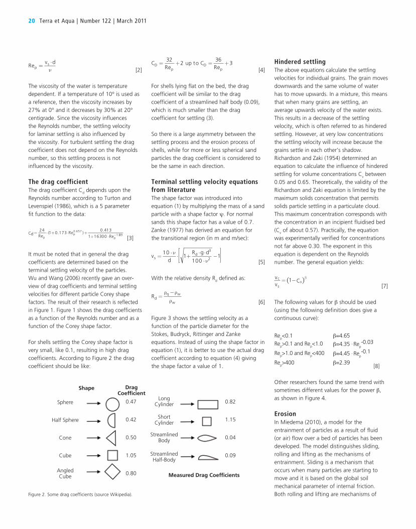
tests are shown in Table I.
A closer look at the data, based on Table I,
shows the following: For the shells on the
0.8 mm sand the d / ks values vary from 1.41-
3.36. The average Shields values found do not
match the corresponding curves, but lead to
slightly lower d / ks values. For example, the
Cross Barred Chione had a Shields value of
0.0378, but based on the d / ks value of 1.41,
a Shields value of about 0.02 would be
expected, a ratio of 1.89. The Coquina Clam
had an average Shields value of 0.0277, but
based on the d / ks value of 2.00 a Shields
value of about 0.015 would be expected,
a ratio of 1.84. The Ponderous Ark had an
average Shields value of 0.0129, but based
on the d / ks value of 3.36 a Shields value of
about 0.008 would be expected, a ratio of
1.61. For the 0.3 mm sand the average ratio
is about 5.5. In other words, the shells require
larger Shields values than corresponding sand
a big difference in the lift coefficient of shells
lying on the bed, between convex upwards
and convex downwards. A convex upwards
shell is like the streamlined half body with a
small drag coefficient. A convex downwards
shell obviously is easy to catch the flow and
start to move, because the drag coefficient is
larger and most probably, the lift coefficient is
much larger. So it will be the convex upwards
shells that armour the bed or the beach.
The question is: What would the drag
coefficient be, based on the experiments of
Dey (2003). Figure 9 shows the Shields
parameters for the three types of shells lying
convex upwards on the bed with two types
of sand, a d50
=0.8 mm and a d50
=0.3 mm,
also the average values are shown. For the
determination of the Shields values, the
definition of the Shields parameter has to be
used more strictly. Often a definition is used
where the Shields parameter equals the ratio
between the shear force and the normal force
on the grain, resulting in a denominator with
the particles diameter.
More strictly, the Shields parameter is the
shear stress divided by the normal stress
and in the case of shells; the normal stress
depends on the average thickness of the
Figure 6. Critical bed shear stress of individual size fractions in a mixture as a function of grain diameter [modified
after van Rijn,(2006) and Wilcock(1993)].
Figure 7. Shape of bivalve
shell (Dey, 2003).
Critical shear stress versus grain diameter
Cri
tica
l bed
sh
ear
stre
ss T
au (
Pa)
Grain diameter d (m)
100
10
1
0.10.0001
d50
=0.67mm, Wilcock (1988)
d50
=1.7mm, Wilcock (1993)
d50
=20mm, Petit (1994)
0.001 0.01 0.1
d50
=0.48mm, Kuhnle (1993)
d50
=2.8mm, Misri (1984)
d50
=0.55mm, Kuhnle (1993)
d50
=5.6mm, Kuhnle (1993)
Shields, E=0.5
d50
=6mm, Wilcock (1993)
d50
=18mm, Wilcock (1993)
Top
Base Plane
Umbo
Ellipse
Base
c
b b1
a = a1
Shell with convex upward condition
Shell with convex downward condition
FL
Fs F
D
FG
Z0
z
u
x
FL
Fs F
D
FG
Z0
z
u
x

How can this critical velocity be combined
with the erosion behavior of shells?
As mentioned above, there are different
models in literature for the critical velocity and
there is also a difference between the critical
velocity and the minimum friction velocity.
However, whatever model is chosen, the real
critical velocity is the result of an equilibrium
of erosion and deposition resulting in a
stationary bed. This equilibrium depends on
the particle size distribution, the slurry density
and the flow velocity. At very low concentra-
tions it is often assumed that the critical
velocity is zero, but based on the theory of
incipient motion, a certain minimum velocity
is always required to erode an existing bed.
The problem can be looked at in two ways:
one can compare the Shields values of the
shells with the Shields values of sand particles
with a diameter equal to the thickness of the
shells, resulting in the factors as mentioned in
the previous paragraph or one can compare
the shear stresses occurring to erode the shells
with the shear stresses required for the sand
beds used. The latter seems more appropriate
because the shear stresses are directly related
to the average velocity above the bed with
the following relation:
ρλρw wu U⋅ = ⋅ ⋅*
2 2
8 [22]
pumping velocity or lowering the concentration
will be enough to start the bed sliding, then
erode the bed and return to stable operation.
With a sand-shell mixture, as described above,
the critical velocity and minimum friction
velocities become time-dependent parameters.
The stochastic nature of the process means
that some fraction of the shells will fall to the
bottom of the pipe. The asymmetry between
deposition and erosion velocity means that
these shells will stay on the bottom, forming
a bed that grows over time, increasing the
critical velocity and minimum friction velocity.
Unless the system is operated with very high
margins of velocity, the new critical velocity
and Vimin
eventually fall within the operating
range of the system, leading to flow instability
and possible plugging.
grains. This effect is larger in the case of shells
on a bed with finer sand particles. The exact
ratios depend on the type of shells.
Critical VelocityA familiar phenomenon in the transport of
sand slurries is critical velocity, the velocity at
which the mixture forms a stationary bed in
the pipeline. As the velocity increases from the
critical, the mixture bed starts to slide along
the bottom of the pipe. As the velocity
increases further the bed begins to erode with
the particles either rolling or saltating along the
top of the bed, or fully suspended in the fluid.
A related concept is that of the minimum
friction velocity, Vimin
, at which the friction in
the pipeline is minimised. At low concentra-
tions the Vimin
may be equal or just above the
critical velocity, but as concentration increases
the critical velocity starts to decrease while the
Vimin
continues to rise. In operational terms, the
Vimin
represents a point of instability, so
pumping systems are generally designed to
maintain sufficiently high velocities that the
system velocity never falls below (or close to)
Vimin
during the operational cycle.
Implicit in most models of slurry transport is
the idea that the system can transition
smoothly in both directions along the system
resistance curves. So if the dredge operator
inadvertently feeds too high of a concentra-
tion, dropping the velocity close to the
minimum friction or even the critical velocity,
he can recover by slowly lowering the mixture
concentration, which in turn lowers the density
in the pipeline and allows the velocity to
recover. Alternatively the operator can increase
the pressure by turning up the pumps to raise
the velocity. In a sand-sized material this works
because the critical and minimum friction
velocities are fairly stable, so raising the
Hydraulic Transport of Sand /Shell Mixtures in Relation with the Critical Velocity 25
Figure 8. Selected samples of bivalve shells.
Figure 9. Shells convex upward.
Non-uniform particle distribution, Shells Convex Upward
Shie
lds
Para
met
er
Re
10-1
10-2
10-3
d/ks=0.50, E=0.625
d/ks=6.00, E=0.920
d/ks=100, E=0.995
d/ks=1.00, E=0.500
d/ks=8.00, E=0.940
d/ks=2.00, E=0.625
d/ks=10.0, E=0.950
d/ks=0.25, E=0.750
d/ks=4.00, E=0.750
d/ks=20.0, E=0.975
100 101 102
Ponderous Arksk=0.8 mm, up
Coquina,sk=0.3 mm, up
Chione average Ponderous Ark average
Chione,sk=0.3 mm, up
Coquina average
Chione,sk=0.8 mm, up
Chione average
Ponderous Arksk=0.8 mm, up
Chione,sk=0.8 mm, up
Ponderous Ark average
Coquina average
Coquina Clam Ponderous Ark Cross Barred Chione
26 Terra et Aqua | Number 122 | March 2011
Where the left hand side equals the bed shear
stress, λ the friction coefficient following from
the Moody diagram and U the average flow
velocity above the bed. The average shear
stresses are shown in Table II.
The Shields values for both sands are about
0.035, resulting in shear stresses of 0.45 Pa
for the 0.8 mm sand and 0.17 Pa for the
0.3 mm sand. The ratios between the shear
stresses required eroding the shells and the
shear stresses required to erode the beds are
also shown in Table II. For the shells laying
convex upwards on the 0.8 mm sand bed
these ratio’s vary from 1.24-1.60, while this is
a range from 2.18-3.41 for the 0.3 mm sand
bed. These results make sense, the shear
stress required for incipient motion of the
shells does not change much because of the
sand bed, although there will be some
reduction for sand beds of smaller particles
owing to the influence of the bed roughness
on the velocity profile according to equation
(14). Smaller sand particles with a smaller
roughness allow a faster development of the
velocity profile and thus a bigger drag force
on the shells at the same shear stress.
The main influence on the ratios is the size of
the sand particles, because smaller particles
require a smaller shear stress for the initiation
of motion.
This is also known from the different models
for the critical velocity, the finer the sand
grains, the smaller the critical velocity. In order
words, the smaller the velocity to bring the
particles in a bed back into suspension. It also
makes sense that the ratio between shell
erosion shear stress and sand erosion shear
stress will approach 1 if the sand particles will
have a size matching the thickness of the
shells and even may become smaller than 1
if the sand particles are bigger than the shells.
Since the velocities are squared in the shear
stress equation, the square root of the ratios
has to be taken to get the ratios between
velocities. This leads to velocity ratios from
1.11-1.26 for the 0.8 mm sand and ratios
from 1.48-1.89 for the 0.3 mm sand.
Translating this to the critical velocity can be
carried out under the assumption that the
critical velocity is proportional to the average
flow velocity resulting in incipient motion.
Although the critical velocity results from an
equilibrium between erosion and deposition
of particles and thus is more complicated,
the here derived ratios can be used as a first
attempt to determine the critical velocities for
a sand bed covered with convex upwards
shells. For the coarser sands (around 0.8 mm)
this will increase the critical velocity by 11%-
26%, while this increase is 48%-89% for the
finer 0.3 mm sand. Even finer sands will have
a bigger increase, while coarser sands will
have a smaller increase.
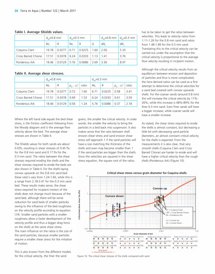
As stated, the shear stress required to erode
the shells is almost constant, but decreasing a
little bit with decreasing sand particle
diameters, an almost constant critical velocity
for the shells is expected. From the
measurements it is also clear, that very
smooth shells (Coquina Clam and Cross
Barred Chione) are harder to erode and will
have a higher critical velocity than the rough
shells (Ponderous Ark) (Figure 10).
Table II. Average shear stresses.
d50
=0.8 mm d50
=0.3 mm
Re*
θ ρw . u
*2 ratio Re
*θ ρ
w . u
*2 ratio
Coquina Clam 19.78 0.0277 0.72 1.60 6.71 0.0225 0.58 3.41
Cross Barred Chione 17.51 0.0378 0.69 1.53 6.24 0.0333 0.61 3.59
Ponderous Ark 18.46 0.0129 0.56 1.24 5.76 0.0086 0.37 2.18
Figure 10. The critical shear stresses of the shells compared with sand.
Critical shear stress versus grain diameter for Coquina shells
Cri
tica
l bed
sh
ear
stre
ss T
au (
Pa)
Grain diameter d (m)
10
1
0.1
0.00001
Shells cu on 0.3 mm sand (CC)
Shells cu on 0.3 mm sand (CBC)
Shells cu on 0.3 mm sand (PA)
0.0001 0.001 0.01
Shells cu on 0.8 mm sand (CC)
Shells cu on 0.8 mm sand (CBC)
Shells cu on 0.8 mm sand (PA)
0.01
CC = Coquina ClamCBC = Cross Barred ChionePA = Ponderous Ark
cu = Convex Upcd = Convex Down
Sand grains
Shells cd on 0.8 mm sand (CC)
Shells cd on 0.8 mm sand (CBC)
Shells cd on 0.8 mm sand (PA)
Shells cd on 0.3 mm sand (CC)
Shells cd on 0.3 mm sand (CBC)
Shells cd on 0.3 mm sand (PA)
Convex down
Convex up
Table I. Average Shields values.
d50
=0.8 mm d50
=0.3 mm d50
=0.8 mm d50
=0.3 mm
Re*
θ Re*
θ d d/ks
d/ks
Coquina Clam 19.78 0.0277 6.71 0.0225 1.60 2.00 5.33
Cross Barred Chione 17.51 0.0378 6.24 0.0333 1.13 1.41 3.76
Ponderous Ark 18.46 0.0129 5.76 0.0086 2.69 3.36 8.97
Hydraulic Transport of Sand /Shell Mixtures in Relation with the Critical Velocity 27
REFERENCES
Dey, S. (2003).Incipient motion of bivalve shells on
sand beds under flowing water. Journal of Hydraulic
Engineering, pp. 232-240.
Di Filice, R. (1999).The sedimentation velocity of
dilute suspensions of nearly monosized spheres.
International Journal of Multiphase Flows 25, pp.
559-574.
Egiazarof, I. (1965).Calculation of non-uniform
sediment concentrations. Journal of the Hydraulic
Division, ASCE, 91(HY4), pp. 225-247.
Fisher, J., Sill, B.and Clark, D. (1983).Organic
Detritus Particles: Initiation of Motion Criteria on
Sand and Gravel Beds. Water Resources Research,
Vol. 19, No. 6., pp. 1627-1631.
Garside, J.and Al-Dibouni, M.(1977).Velocity-
Voidage Relationships for Fluidization and
Sedimentation in Solid-Liquid Systems. 2nd Eng.
Chem. Process Des. Dev., 16, 206.
Miedema, S. (2010). Constructing the Shields curve,
a new theoretical approach and its applications.
WODCON XIX (p. 22 pages). Beijing, September
2010: WODA.
Miller, R.and Byrne, R.(1966).The angle of repose for
a single grain on a fixed rough bed. Sedimentology
6, pp. 303-314.
Reichardt, H.(1951).Vollstandige Darstellung der
Turbulenten Geswindigkeitsverteilung in Glatten
Leitungen. Zum Angew. Math. Mech., 3(7), pp.
208-219.
Richardson, J.and Zaki, W. (1954). Sedimentation &
Fluidization: Part I. Transactions of the Institution of
Chemical Engineering 32, pp. 35-53.
Rijn, L.van (2006). Principles of sediment transport in
rivers, estuaries and coastal areas, Part II:
Supplement 2006. Utrecht & Delft: Aqua
Publications, The Netherlands.
Rowe, P. (1987). A convenient empirical equation
for estimation of the Richardson-Zaki exponent.
Chemical Engineering Science Vol. 42, no. 11, pp.
2795-2796.
Turton, R. and Levenspiel, O. (1986). A short note
on the drag correlation for spheres. Powder
technology Vol. 47, pp. 83-85.
Wallis, G. (1969). One Dimensional Two Phase Flow.
McGraw Hill.
Wiberg, P. L. and Smith, J. D. (1987A). Calculations
of the critical shear stress for motion of uniform and
heterogeneous sediments. Water Resources
Research, 23 (8), pp. 1471–1480.
Wilcock, P. (1993). Critical shear stress of natural
sediments. Journal of Hydraulic Engineering Vol.
119, No. 4., pp. 491-505.
Wu, W. and Wang, S. (2006). Formulas for sediment
porosity and settling velocity. Journal of Hydraulic
Engineering, 132(8), pp. 858-862.
Zanke, U.C. (1977). Berechnung der Sinkgeschwindig
keiten von Sedimenten. Hannover, Germany:
Mitteilungen Des Francius Instituts for Wasserbau,
Heft 46, seite 243, Technical University Hannover.
CONCLUSIONS
The critical velocity for the hydraulic transport
of a sand-water mixture depends on a number
of physical processes and material properties.
The critical velocity is the result of equilibrium
between the deposition of sand particles and
the erosion of sand particles. The deposition
of sand particles depends on the settling
velocity, including the phenomenon of
hindered settling as described in this article.
The erosion or incipient motion of particles
depends on equilibrium of driving forces, like
the drag force, and frictional forces on the
particles at the top of the bed. This results in
the so-called friction velocity and bottom shear
stress. Particles are also subject to lift forces
and so-called Magnus forces, owing to the
rotation of the particles. Particles that are
subject to rotation may stay in suspension
owing to the Magnus forces and they do not
contribute to the deposition. From this it is
clear that an increasing flow velocity will result
in more erosion, finally resulting in hydraulic
transport without a bed. A decreasing flow
velocity will result in less erosion and an
increasing bed thickness, resulting in the
danger of plugging the pipeline.
Shells lying convex upwards on the bed in
general are more difficult to erode than sand
particles, as long as the sand particles are
much smaller than the thickness of the shells.
The shells used in the research had a thickness
varying from 1.13 to 2.69 mm. So the shells
armour the bed and require a higher flow
velocity than the original sand bed. Now as
long as the bed thickness is not increasing,
there is no problem, but since hydraulic
transport is not a simple stationary process,
there will be moments where the flow may
decrease and moments where the density may
increase, resulting in an increase of the bed
thickness. Since the shells are armouring the
bed, there will not be a decrease of the bed
thickness at moments where the flow is higher
or the density is lower, which would be the
case if the bed consists of just sand particles.
This means a danger of a bed thickness
increasing all the time and finally plugging the
pipeline. The question arises, how much does
one have to increase the flow or flow velocity
in order to erode the top layer of the bed
where the shells are armouring the bed.
From the research of Dey (2003) it appears
that the bottom shear stress to erode the
shells varies from 0.56-0.72 Pa for a bed with
0.8 mm sand and from 0.37-0.61 Pa for a bed
with 0.3 mm sand. It should be noted that
these are shear stresses averaged over a large
number of observations and that individual
experiments have led to smaller and bigger
shear stresses. So the average shear stresses
decrease slightly with a decreasing sand
particle size owing to the change in velocity
distribution. These shear stresses require
average flow velocities that are 11%-26%
higher than the flow velocities required to
erode the 0.8 mm sand bed and 48%-89%
higher to erode the 0.3 mm sand bed. From
these numbers it can be expected that the
shear stresses required to erode the shells,
match the shear stresses required to erode a
bed with sand grains of 1-1.5 mm and it is
thus advised to apply the critical velocity of
1-1.5 mm sand grains in the case of dredging
a sand containing a high percentage of shells,
in the case the shells are not too fragmented.
Top Related