


Languages
Pages
Legal

Hours Off the Clock
by
Andrew S. Green Cornell University and
U.S. Census Bureau
CES 17-44 June, 2017
The research program of the Center for Economic Studies (CES) produces a wide range of economic analyses to improve the statistical programs of the U.S. Census Bureau. Many of these analyses take the form of CES research papers. The papers have not undergone the review accorded Census Bureau publications and no endorsement should be inferred. Any opinions and conclusions expressed herein are those of the author(s) and do not necessarily represent the views of the U.S. Census Bureau. All results have been reviewed to ensure that no confidential information is disclosed. Republication in whole or part must be cleared with the authors. To obtain information about the series, see www.census.gov/ces or contact J. David Brown, Editor, Discussion Papers, U.S. Census Bureau, Center for Economic Studies 5K034A, 4600 Silver Hill Road, Washington, DC 20233, [email protected]. To subscribe to the series, please click here.

Abstract
To what extent do workers work more hours than they are paid for? The relationship between hours worked and hours paid, and the conditions under which employers can demand more hours “off the clock,” is not well understood. The answer to this question impacts worker welfare, as well as wage and hour regulation. In addition, work off the clock has important implications for the measurement and cyclical movement of productivity and wages. In this paper, I construct a unique administrative dataset of hours paid by employers linked to a survey of workers on their reported hours worked to measure work off the clock. Using cross-sectional variation in local labor markets, I find only a small cyclical component to work off the clock. The results point to labor hoarding rather than efficiency wage theory, indicating work off the clock cannot explain the counter-cyclical movement of productivity. I find workers employed by small firms, and in industries with a high rate of wage and hour violations are associated with larger differences in hours worked than hours paid. These findings suggest the importance of tracking hours of work for enforcement of labor regulations. *
*Any opinions and conclusions expressed herein are those of the author and do not necessarily represent the views of the U.S. Census Bureau. All results have been reviewed to ensure that no confidential information is disclosed. This paper has benefited greatly from comments and suggestions of John Abowd, Richard Mansfield, Karel Mertens, Lars Vilhuber, Kathryn Edwards, Hautahi Kingi, Mark Kutzbach, Sabrina Pabilonia (discussant), Jim Spletzer, as well as seminar participants of the Labor Dynamics Institute, Cornell Labor Work in Progress Seminar, Census CES Brown Bag Seminar, Census-BLS conference, and Cornell Labor Seminar. I acknowledge the use of the Cornell ECCO computing cluster. All errors are my own. E-mail: [email protected].
1 Introduction
How many hours do people work? Myriad government surveys of hours worked from
households, and hours paid from establishments exist to answer this question, though each
has drawbacks.1 How much time employees spend at work, and whether this time is ex-
plicitly tracked and bargained for, is neither well measured nor understood. In addition to
worker welfare, the difference between hours paid and hours worked has implications for the
cyclical movement of productivity and wages. Specifically, off-the-clock work2 is a possible
explanation for the change in productivity from pro-cyclical to counter-cyclical during the
last three business cycles.
The difficulty measuring work off the clock is not only a concern for economists and
government statistical agencies, it is also essential for the understanding of firm profits and
worker welfare. In the last few years, stories in the popular press recount hourly workers
asked to show up to work and told to wait – without pay – until demand picked up.3
Other times wage theft was more explicit, with employers doctoring reports of hours worked
to show a higher hourly wage,4 or workers asked to keep working after they had clocked
out.5 Salaried workers, too, were frequently asked to pick up some or all of the work for
colleagues who were laid off.6 The various stories are not uniform to all workers, but they
all point to the various dynamics that influence bargaining over time in the workplace and
how much work time happens off the clock. Empirical research that documents off-the-clock
work specifically, and labor compliance more broadly, is growing, but little research using
representative government datasets exists.7
In this study, I examine how shocks to labor demand and firm characteristics influence
work off the clock. I construct a unique dataset of survey responses of hours worked from
the U.S. Census Bureau’s American Community Survey (ACS) with administrative data
on hours paid from the U.S. Census Bureau’s Longitudinal Employer-Household Dynamics
(LEHD) program. I adjust the ACS survey weights to account for the shift in frame, so the
analysis sample remains representative. To the best of my knowledge, this is the first study
1Establishment surveys of hours paid likely miss long hours for salaried workers and off-the-clock work.Household surveys rely on accurate recall of all jobs.
2I will refer to “off-the-clock” work synonymously with ”the difference between hours worked and hourspaid”. I use this phrase only for its brevity.
3“More Workers Are Claiming ‘Wage Theft’.” The New York Times, Aug. 31, 2014.4“Squeezed garment factories use check cashing services to mask true wages, workers say.” The Los
Angeles Times, Jul. 30, 2016.5“Nearly 10,000 Chipotle Workers Join Class Action Wage Lawsuit.” The New York Daily News, Aug.
30, 2016.6“All Work and No Pay: The Great Speedup.” Mother Jones, July/August, 2011.7Bernhardt et al. (2013) and Milkman et al. (2012) are recent examples.
2
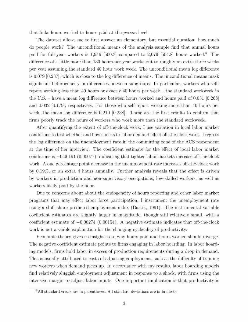
that links hours worked to hours paid at the person-level.
The dataset allows me to first answer an elementary, but essential question: how much
do people work? The unconditional means of the analysis sample find that annual hours
paid for full-year workers is 1,946 [500.3] compared to 2,079 [504.8] hours worked.8 The
difference of a little more than 130 hours per year works out to roughly an extra three weeks
per year assuming the standard 40 hour work week. The unconditional mean log difference
is 0.079 [0.237], which is close to the log difference of means. The unconditional means mask
significant heterogeneity in differences between subgroups. In particular, workers who self-
report working less than 40 hours or exactly 40 hours per week – the standard workweek in
the U.S. – have a mean log difference between hours worked and hours paid of 0.031 [0.268]
and 0.032 [0.179], respectively. For those who self-report working more than 40 hours per
week, the mean log difference is 0.210 [0.238]. These are the first results to confirm that
firms poorly track the hours of workers who work more than the standard workweek.
After quantifying the extent of off-the-clock work, I use variation in local labor market
conditions to test whether and how shocks to labor demand effect off-the-clock work. I regress
the log difference on the unemployment rate in the commuting zone of the ACS respondent
at the time of her interview. The coefficient estimate for the effect of local labor market
conditions is −0.00191 (0.00077), indicating that tighter labor markets increase off-the-clock
work. A one percentage point decrease in the unemployment rate increases off-the-clock work
by 0.19%, or an extra 4 hours annually. Further analysis reveals that the effect is driven
by workers in production and non-supervisory occupations, low-skilled workers, as well as
workers likely paid by the hour.
Due to concerns about about the endogeneity of hours reporting and other labor market
programs that may effect labor force participation, I instrument the unemployment rate
using a shift-share predicted employment index (Bartik, 1991). The instrumental variable
coefficient estimates are slightly larger in magnitude, though still relatively small, with a
coefficient estimate of −0.00274 (0.00154). A negative estimate indicates that off-the-clock
work is not a viable explanation for the changing cyclicality of productivity.
Economic theory gives us insight as to why hours paid and hours worked should diverge.
The negative coefficient estimate points to firms engaging in labor hoarding. In labor hoard-
ing models, firms hold labor in excess of production requirements during a drop in demand.
This is usually attributed to costs of adjusting employment, such as the difficulty of training
new workers when demand picks up. In accordance with my results, labor hoarding models
find relatively sluggish employment adjustment in response to a shock, with firms using the
intensive margin to adjust labor inputs. One important implication is that productivity is
8All standard errors are in parentheses. All standard deviations are in brackets.
3
pro-cyclical.
In light of the result that off-the-clock work is probably pro-cyclical and driven by low-skill
workers, I test for explanations centered on labor compliance. Although still an emerging
literature, research finds that smaller firms are much less likely to comply with labor regu-
lations. Consistent with this literature, I find that firms in the smallest firm size category,
0-19 employees, report higher incidence of work off the clock compared to firms with greater
than 2,500 employees with a log difference of 0.0231 (0.0053). I find the effect is driven
by production and non-supervisory workers who are likely paid on an hourly basis. I also
show that off-the-clock work is concentrated in industries where wage and hour violations
are prevalent.
The results on the cyclical nature of off-the-clock work challenge a recent literature testing
for efficiency wage explanations for the counter-cyclical nature of productivity. Lazear et al.
(2015) and Burda et al. (2016) use local labor market variation to test for greater effort
in slack labor markets. Unlike this paper, they do not look for work off the clock, rather
they model greater effort per unit of time at work. The empirical strategy in Lazear et al.
(2015) employs data on a single firm with a wide geographic dispersion of establishments,
that tracks piece-rate production. Burda et al. (2016) use an empirical strategy similar to
Lazear et al. (2015), but they use the American Time Use Survey to measure time at work
actually working, which is a proxy for greater effort. In contrast to my paper, both studies
find evidence that greater local labor market slack is associated with greater effort provision.
My estimates quantifying off-the-clock work and its implications for productivity statis-
tics confirm several previous papers. Aaronson and Figura (2010) also attempt to use off-
the-clock work to explain the counter-cyclical turn in productivity. They construct time
series of hours worked and hours paid from the Current Population Survey and the Current
Establishment Statistics, respectively. Although they must rely on aggregate data, they
too find little evidence for off-the-clock work biasing productivity estimates. Eldridge and
Pabilonia (2010) use the American Time-Use Survey (ATUS) and the Work Schedules and
Work at Home Supplement to the Current Population Survey to address whether the inci-
dence of working from home biases productivity statistics. They find over the time span of
their sample that unpaid work at home sometimes overstates, and other times understates
the hours levels used in the BLS productivity series. The bias in all cases is exceedingly
small, and unlikely to bias productivity statistics.
Recent research uses survey and administrative data to document non-compliance with
minimum wage laws, overtime regulations, and work off the clock. Bernhardt et al. (2013)
and Milkman et al. (2012) use the 2008 Unregulated Worker Survey, and they find that job
and employer characteristics are responsible for much of the variation in noncompliance. Ji
4

and Weil (2015) use a unique dataset of franchisor- and franchisee-owned establishments
matched to Wage and Hour Administration investigations. They find that franchisee-owned
establishments are more likely to commit wage and hour violations. My estimates of off-
the-clock work are broadly consistent with this literature. Off-the-clock work is most con-
centrated in small firms, and within industries that disproportionately employ low-wage
workers.
Since applied economics is moving towards the use of large administrative datasets, the
results of my study also suggest caution when using administrative data to measure hours.
Few studies have explicitly compared employer and employee reports of hours worked.9 One
exception is Mellow and Sider (1983) who use an employer validation supplement to the CPS
to glean employer and worker responses to myriad questions. For hours, they find worker
reports exceed employer reports by 3.9%, which is substantially less than the 7.9% in the
preferred specification. The difference is likely due to the analysis sample in this study, which
only considers full-time, full-year workers. Lastly, this study contributes to the growing body
of research which uses administrative data to validate survey data.10
2 Hours Divergence: Theory and Implications
I construct a unique dataset of hours worked and hours paid in order to try to infer
the causes, incidence, and implications of off-the-clock work. A natural question quickly
arises: why should we expect the difference between hours paid and hours worked to reflect
anything but errors in reporting? Although measurement error is no doubt present, this
section lays out established economic theories of why hours paid may diverge from hours
worked. The first two theories provide opposing predictions for the movement of off-the-
clock work over the business cycle. Efficiency wage models predict workers will exert more
effort – greater hours worked compared to hours paid – when labor markets are slack. In
contrast, theories of labor hoarding predict the opposite relationship between off-the-clock
work and macroeconomic conditions.
In addition to cyclical theories of why hours paid may diverge from hours worked, I
view the difference through an older literature on labor regulation compliance. In these
models the firm’s profit motive leads them to skirt labor laws to realize greater profits.
Firms must weigh the higher profit of non-compliance against the probability of getting
caught and the penalties of non-compliance. The Great Recession and the ensuing debate
9See Duncan and Hill (1985), Bound and Krueger (1991), Bound et al. (1994), and Bound et al. (2001)for an overview.
10See Abraham et al. (2013) and Abowd and Stinson (2013).
5
about the declining wages and working conditions of low wage workers have brought this
topic to greater prominence in the media. Better administrative data on employment, firms,
and greater transparency and data around compliance investigations have invigorated this
literature.
2.1 Efficiency Wages & Labor Hoarding
In efficiency wage theories of the labor market, workers would like to avoid being laid
off, and firms would like workers to exert effort. At least since Kalecki (1943), who noted
“under a regime of permanent full employment, the ‘sack’ would cease to play its role as a
disciplinary measure,” economists have studied the relationship between the labor market
and worker effort. More recent discussions of efficiency wage models pick up with Shapiro
and Stiglitz (1984). In their model, the firm’s production depends on worker effort, which
firms cannot perfectly monitor. Workers would prefer to shirk rather than exert effort. Firms
offer wages in excess of the market clearing rate in order to induce effort. The theory provides
a succinct explanation of involuntary unemployment.
The model relevant for the empirical tests in this paper does not provide a theory of
unemployment. Although similar, the key is the cost to firms of replacing workers, or
alternatively the cost to workers of finding a new job.11 The driving variable is the tightness
of the labor market. As the labor market becomes more slack, the cost of job loss increases
due to worse prospects of finding a new job. Workers exert extra effort in the form of more
hours worked in order to signal their worth to employers and avoid a lay off. In the case
of hourly workers, this may be explicit off-the-clock work. For salaried workers, these extra
hours are in excess of what is “normal” under more favorable labor market conditions.
In contrast, labor hoarding theories predict that labor productivity should be pro-cyclical
Popular in the 1960s,12 theories of labor hoarding hold that firms retain more workers in
a downturn than production explicitly requires.13 Firms may have incurred the costs of
training workers to their specific production technology, or highly skilled workers may be
scarce. In both cases firms would rather not risk laying off workers who may be difficult
to rehire, or pay the upfront cost to train new hires. To meet reduced production targets,
firms then adjust hours worked in order to meet production targets. If firms choose to keep
a worker’s labor earnings constant, hours paid may exceed hours worked. The implication
for labor hoarding theory is that productivity will decline during downturns as hours paid
11Rebitzer (1987) is the most relevant paper capturing the former case. See Appendix A for the lattercase.
12See Oi (1962) & Fair (1969).13Biddle (2014) provides a nice history of the literature.
6

stays relatively constant and production declines.14
More modern theories of labor demand would interpret labor hoarding through the lens
of adjustment costs. Firms face an explicit cost to adjusting their labor on the extensive
margin. Depending on the size and functional form of the costs, firms will not always adjust
employment to its optimal level in response to a shock. Firms will adjust employment less
than in the absence of adjustment costs and use hours to adjust total labor input to its
optimal level.15
Efficiency wage and labor hoarding models are not mutually exclusive. In fact, both are
likely present in any given employment relationship. The empirical approach employed in
this study will not be able to separately identify the two. The empirical analysis in this
paper serves to answer the question of which is more salient for interpreting the cyclical
changes in productivity and real wages. It should therefore help guide macroeconomists on
how best to incorporate the costs of separations to workers and firms in their models.
2.2 Labor Regulation Compliance
In addition to the cyclical forces, explicit failure to comply with labor regulations is
another reason why hours worked may exceed hours paid. The Fair Labor Standards Act
(FLSA), enacted in 1938, established the federal minimum wage, and effectively enshrined
the 40-hour work week by requiring overtime pay of time-and-a-half for all hours worked over
40 in a week. The literature on compliance with the FLSA centers on the firm. Firms weigh
their profits from compliance against their expected profits from non-compliance (Ashenfelter
and Smith, 1979). The model leads to the conclusion that firms need to take into account
the costs of noncompliance, the odds of getting caught, the elasticity of labor demand, and
the spread between the prevailing wage and the minimum wage in a given industry.16
Recent empirical research finds firm and job characteristics such as firm size, industry,
and non-hourly pay arrangements drive non-compliance with labor regulations. Bernhardt
et al. (2013) conduct a survey of low-wage workers in major American metropolitan areas.
They survey non-compliance, but also collect detailed worker and firm characteristics. They
have two important findings. First, larger firms (greater than 100 employees) are less likely
to commit labor violations compared to firms less than 100 employees. Second, they find that
non-hourly workers are more likely to incur wage and hour violations, and that off-the-clock
work is more prevalent than straight minimum wage violations.
14Employer reports of hours paid are the main input to the BLS productivity series, while hours workedis the variable of economic interest. See Eldridge and Pabilonia (2010).
15See Cooper et al. (2007), Caballero et al. (1997), and Hamermesh (1989) for more recent examples.Appendix A describes the theory in more detail.
16See also Chang and Ehrlich (1985), and Basu et al. (2010).
7
There are a few reasons why smaller firms may be more likely to commit labor viola-
tions. First, small firms have fewer establishments and therefore stand less of a chance of
getting caught for noncompliance if enforcement is equally probable for all establishments.
Second, small firms are less likely to have in-house expertise (human resource departments)
to negotiate regulations (Mendeloff et al., 2006), and are less likely to be unionized.17 Small
firms tend to have less capital and rely more heavily on labor inputs. Thus, if they are going
to cut costs, it will likely be on labor.18 Finally, the fact that small firms have less capital
reduces the costs of non-compliance. Firms that owe back wages have the opportunity to
declare bankruptcy and forsake owed back wages. The less capital a firm has, the smaller
the costs to bankruptcy.19
The measurement of hours is often an important determinant for wage and hour viola-
tions. Recent changes in technology and the organization of firms make measuring hours a
challenge in wage and hour compliance. Tracking hours is important for assessing off-the-
clock work, overtime violations, and many minimum wage violations when workers are not
paid by the hour. New technology makes assessing hours more difficult as more work takes
place at home with computers outside of normal business hours. In addition, tracking hours
for workers who may work at multiple work sites and who may be employed by third party
entities pose new challenges to enforcement agencies (Weil, 2010). In short, the measurement
of hours is invaluable for effective enforcement of wage and hour violations, and it constitutes
a significant margin through which many violations take place.
3 Data
Making inferences about the differences between hours paid and hours worked requires
data on both variables. Previous estimates of the divergence between hours paid and hours
worked relied on aggregated time series data. An innovation of this paper is to link the
two variables at the person level. To the best of my knowledge, this is the first paper to
explicitly link workers’ reports of hours worked to employers’ reports of hours paid for a
representative sample of workers. The result is a survey response of hours worked and the
corresponding administrative reports of hours paid from the survey respondent’s employers.
To construct this difference measure, I use administrative data of hours paid from the U.S.
Census Bureau’s Longitudinal Employer-Household Dynamics (LEHD) program linked to
survey responses to the American Community Survey from the U.S. Census Bureau.
17Weil (1991) shows labor unions correlate with OHSA investigations.18See Ji and Weil (2015) for a similar discussion on franchisee vs. franchisor labor compliance.19“Few California workers win back pay in wage-theft cases.” The Los Angeles Times, April 6, 2015.
8

The LEHD is an administrative file system of linked employer-employee data derived
from state unemployment insurance systems. The data result from a unique partnership
between states and the U.S. Census Bureau, where the states provide the Census Bureau
quarterly extracts of earnings records from their unemployment insurance systems. The core
file is a job-based frame, named the Employment History File (EHF), with a unique record
represented by a person-firm-year-quarter link with any positive earnings in a given quarter,
which covers approximately 95% of all jobs in the United States.20 The fact that the LEHD
comprises a near-universe of jobs and employer-employee links is important as it lets me
account for hours paid in all jobs of the survey respondent, as well as providing the link to
survey data for hours worked.
In addition to quarterly earnings, four states provide quarterly reports of hours paid.
The states are Washington, Minnesota, Rhode Island, and Oregon.21 The quarterly hours
data allow me to construct a measure of total hours paid across all jobs in the previous year
for each person. The final LEHD sample consists of a person-level measure of all jobs paid
in the previous year for each quarter from 2010 to 2013 for these states.22
Data on hours worked come from the U.S. Census Bureau’s American Community Survey
(ACS). The American Community Survey is a rolling monthly survey of 3.5 million house-
holds each year. The ACS replaced the Census long form after the 2000 census and as such,
it asks questions on housing, demographic, and economic topics. I focus on the questions on
weeks paid in the past year and the usual weekly hours worked. When combined, the two
variables allow me to construct a measure of usual hours worked in the past year across all
jobs from the perspective of the employee.
A point of clarification is needed regarding paid weeks worked for the annual hours worked
measure. The ACS hours worked measure conflates both hours paid and hours worked due
to the weeks worked variable including paid leave. I construct annual hours worked as the
product of usual weekly hours and weeks worked. The ACS measure of annual hours worked
includes some weeks for which the worker was paid, but for which no work was done. I do
not adjust for this in what follows because both LEHD and ACS include paid leave. The
difference in the annual hours measure therefore lets usual weekly hours drive the variation in
the difference between the two measures. Alternatively, both measures could be adjusted to
20 Self-employed workers are not currently incorporated into the LEHD. For a full description of theLEHD infrastructure files see Abowd et al. (2009).
21There does not appear to be an explicit administrative reason why some states collect hours paid inaddition to quarterly earnings.
22The states vary considerably with respect to the time of reporting. Internal rules of the LEHD programdictate that at least three states must be used for any released results, which limits the analysis to begin in2009 when Rhode Island first begins reporting hours until 2014 quarter one, which is the most recent hoursdata available for all states.
9
account for weeks worked rather than weeks paid. Because I am interested in the difference
between the two measures, adjusting both down by the same amount will not influence the
final measure of work off the clock. All statistics showing annual hours levels reflect the lack
of adjustment.
3.1 Sample Construction
For the final merged ACS-LEHD analysis sample, I first separately prepare ACS respon-
dents and create an analogous person-year-quarter frame for the LEHD. The ACS prepa-
ration begins by attaching a protected identification key (PIK) to each ACS respondent.
A PIK is a person-level identifier that allows one to link ACS responses to other individual
datasets within the U.S. Census Bureau.23 Using an internal crosswalk, I link ACS responses
from 2010 to 2013. For each year, an ACS respondent links to a PIK at rates between 91%
and 94% per year. After deduplicating records within a year, I am left with 18.3 million
ACS responses.
I merge the person-year-quarter LEHD frame and the ACS to create the final analysis
dataset. The resulting sample contains 571,000 records. The small sample is a result of
limiting the sample of ACS respondents to those who have positive hours paid in the previous
year in the LEHD hours-reporting states from the time of their ACS interview. I further
restrict the sample to ensure that the LEHD and the ACS frames accord as close as possible.
For consistency with the LEHD, I restrict ACS respondents to those age sixteen and over,
and I require that they have no jobs in other states over the previous year by consulting
the standard LEHD EHF, which includes all available states.24 Using the ACS-reported
dominant job, I exclude federal government employees.25 I use the ACS reported residence
and exclude all respondents who neither live in an hours reporting state, nor in a border
state. It is perfectly reasonable for an ACS respondent living in North Dakota, for example,
to work in Minnesota. As a result of these restrictions, I reduce the sample to 438,000
observations.
The final sample contains additional restrictions to negate any anticipated frame differ-
ences, which could lead to biased measurement of work off the clock. I restrict the sample
to records who report working a full year (50-52 weeks) in the ACS, and who report positive
23See Wagner and Layne (2014) for a description of the U.S. Census Bureau’s PIK assignment process.24I also exclude respondents for whom I find jobs with zero or missing hours data. This is evidence of
unit non-response and would bias measures of work off the clock.25The ACS-reported dominant job does not conform to the definition of a dominant job in the LEHD.
For the ACS, the dominant job is the main job in the week prior to the ACS response. Given the stabilityof federal jobs in general, and the high tenure of my final sample, I use the two definitions interchangeably.Checks for consistency find a high degree of agreement.
10

hours in the LEHD for every quarter in the past year. This restriction is reasonable for
a few reasons. First, the ACS sample restriction narrows weeks worked considerably. The
weeks worked variable in ACS is binned, and the bins become coarser the fewer weeks one
works.26 The LEHD restriction to working in the reference quarter as well as the preceding
four quarters simply ensures consistency with the ACS. Finally, I drop observations where
usual weekly hours is imputed, and observations where workers receive more than 20 percent
of their income from self-employment earnings as reported on the ACS. The final dataset
contains 218,000 records.
In order for the final analysis sample to remain representative of the United States pop-
ulation, I adjust the ACS sample weights. When I merge the ACS to the LEHD universe
of job records, the ACS weights are no longer representative of the U.S. population due
to differences in frame. I first use inverse probability weighting to adjust the ACS sample
weights for PIKs missing at random in the sense of Rubin (1987).27 Second, I adjust the
sample weights to match national demographic characteristics in the 2009-2013 ACS for full-
year workers excluding federal employees. I adjust based on age, gender, race/ethnicity, and
education. The resulting sampling weights allow for inferences about the population after
linking the ACS to a different universe.
3.2 Variable Construction
I create the final total for hours paid from the LEHD over the previous year by summing
hours over jobs and weighting the interview quarter and ending quarter by the ACS interview
date. For person i employed at job j at any year-quarter t between 2010 and 2013, define
hj(i),t as the gross quarterly hours for person i in job j in quarter t. I consider only LEHD
jobs between the quarter of the ACS interview (t), and four quarters prior (t− 4), inclusive.
Total hours paid over the previous year therefore include five quarters of data, which is one
too many. To calculate the final annual hours paid in the LEHD over the previous year from
the survey interview date, I sum hours over all jobs, and take a weighted average of hours
in the interview quarter and the last quarter,
Hi,lehd = (1− ρ)
(∑i∈J
hj(i),t−4
)+
(3∑
t=1
∑i∈J
hj(i),t−k
)+ ρ
(∑i∈J
hj(i),t
). (1)
26There is research pointing to quality problems in hours worked for the ACS for part-time workers(Baum-Snow and Neal, 2009). I include full-year part-time workers, though all results are robust to theirexclusion with some loss of precision.
27This is also known as missing conditional on observable covariates. See appendix B for details on inverseprobability weighting.
11

The first term on the right-hand side of equation 1 is the sum of all hours paid to
respondent i across all jobs J in which the respondent worked in period t − 4. This sum
is multiplied by the weight 1 − ρ. The middle term is the sum of hours paid at all jobs in
the three quarters immediately preceding the interview quarter. The last term is the sum of
hours across all jobs in the interview quarter multiplied by weight ρ. The weights are based
on the percentage of the interview quarter in scope for the total hours calculation.28
To construct annual hours worked in the ACS, I assume that usual weekly hours is
equivalent to average weekly hours and then multiply usual weekly hours by 50, 51 and
52 weeks to get three measures of annual hours worked. Table 1 provides statistics for
annual hours worked assuming a 52 week work year. This is my preferred hours measure for
several reasons. First, the final sample contains workers with relatively high tenure (over six
years), and I perform checks for continuous employment in the LEHD over the previous four
quarters from the reference quarter. Second, the ACS asks for usual weeks worked including
paid sick days, paid vacation, and military service. Given checks for continuous employment
and because the ACS weeks worked question includes paid leave, 52 weeks seems the most
reasonable measure of weeks paid that accords with the LEHD.
The final dependent variable of interest is the log difference between annual hours worked
from the ACS, and total hours paid over the previous year from the LEHD. Recall that the
sample is restricted to full-year workers, and that ACS weeks worked is binned for full-
year workers. Denote the annual ACS hours measure Hwi,acs where w ∈ {50, 51, 52} is the
possible weeks worked. The annual LEHD hours measure is denoted Hi,lehd. The measure of
difference between hours worked and hours paid is ywi = ln(Hwi,acs)− ln(Hi,lehd). I construct
the log difference for all three ACS measures of ACS annual hours. I then winsorize at the
5% and 95% level in order to mitigate bias induced by extreme outliers.29
Demographic, firm, and job characteristics come from a combination of the ACS and the
LEHD. Many characteristics are available in both the LEHD and the ACS. I use the ACS for
demographic characteristics, which are occasionally imputed in the LEHD. For the residence,
I use the ACS reported residence. The LEHD residence is from a fixed time period each year,
and will not necessarily correspond to the residence at the time of ACS interview. I use firm
characteristics from the LEHD dominant job30 as it comes from an administrative source
and best hues towards my preferred definition of a dominant job. I make use of whether or
28For example, if an ACS respondent completed the survey on May 10th, the weight assigned to theinterview quarter would be equal to the 40 days in the quarter divided by 91, which is total days in thesecond quarter. The weight on the end month is simply one minus the interview quarter weight.
29The following analysis has also been carried out with a dependent variable winsorized at the 1% and99%. Results are qualitatively unchanged.
30I define the LEHD dominant job as the job with the most hours paid in the three quarters which liecompletely within the preceding year from the date of the ACS interview.
12

Table 1: Summary Statistics for Analysis Sample
mean sd
ACS annual hours (52 Weeks) 2,079 500.3LEHD annual hours 1,946 504.8Annual hours error (50 weeks, ACS) 0.030 0.251Annual hours error (51 weeks, ACS) 0.055 0.241Annual hours error (52 weeks, ACS) 0.079 0.237
Firm/Job Characteristics
Unemployment rate (%) 7.354 1.901Private, for-profit firm 0.743 0.437Supervisory, Non-production 0.275 0.447Top Quartile, Liklihood Not Paid by Hour 0.277 0.448Dominant job tenure (quarters) 26.96 21.0
Demographic Characteristics
Age 42.30 12.87Male 0.519 0.500Non-white 0.239 0.426Bachelor’s degree or higher 0.325 0.468
Notes: N = 218, 000, with 58 commuting zones. Annual hourserror is the difference between log hours worked in the ACS andlog hours paid from the LEHD. The ACS hours paid measure isdefined by multiplying the usual weekly hours by the number ofweeks paid. Supervisory workers adhere to the Bureau of LaborStatistics definition of supervisory or non-production workers. Seetext for details.
13

not a worker is paid by the hour. This is not available in either the ACS or LEHD.31 I use
the Current Population Survey to impute hourly/non-hourly pay using industry, occupation,
and earnings according to the ACS. I then bin the resulting probability of non-hourly pay
into quartiles for use in the empirical analysis.32
3.3 Summary Statistics
Summary statistics of the mean and standard errors for the final sample are found in Table
1. The first two lines give the summary statistics for estimates of annual hours worked from
the ACS and annual hours paid from the LEHD. The bottom panel displays demographic
characteristics used to match the analysis sample to the U.S. population. The restriction to
full-year workers is perhaps the most salient for what follows. Note that the average tenure
in LEHD dominant jobs is a little under 27 quarters, or slightly greater than 6.5 years.
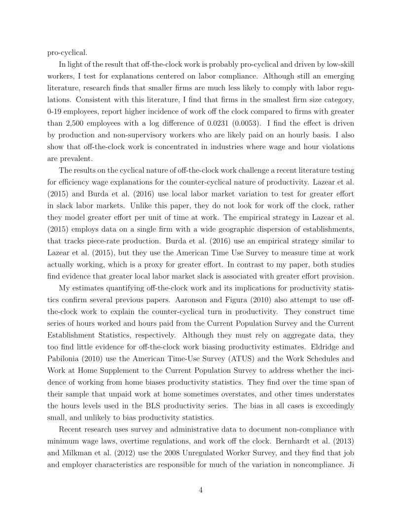
Figure 1 shows the full distribution of the difference in log hours worked from log hours
paid. I use my preferred ACS hours worked measure, which assumes 52 paid weeks. The
distribution is centered slightly to the right of zero, but it is highly skewed with a long right
tail implying many more people report working more than their employers say they do. Note
that the distribution is winsorized at the 95% level, which slightly truncates the right tail of
the distribution, but analysis relaxing the winsorization to the 99% level does not alter the
results.
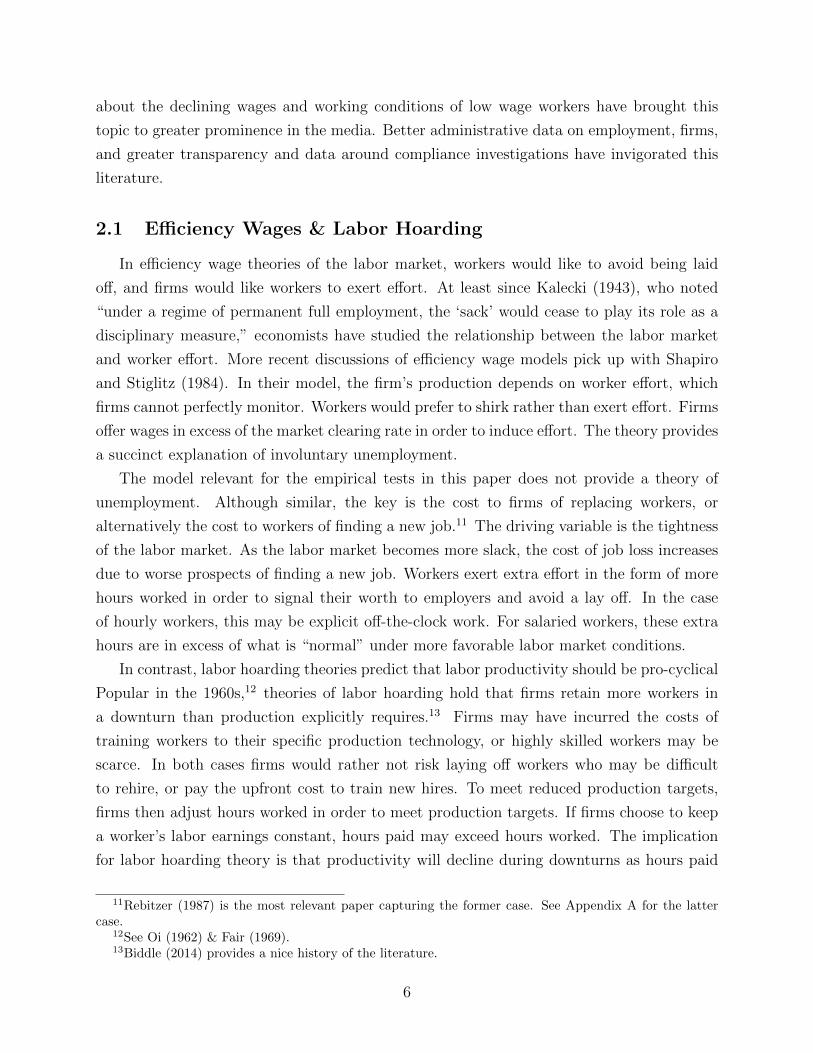
Partitioning the distribution by a few characteristics reveals large differences between
hours worked and hours paid, particularly for those who report working more than 40 hours
per week. Figure 2 shows the large disparity in work off the clock by workers who self-
report working more than 40 hours per week. The figure partitions the distribution of the
difference in log hours into those who self-report usually working less than 40 hours per
week (top panel), those who usually work 40 hours per week (middle panel), and those who
usually work more than 40 hours per week (bottom panel). The difference is stark. Those
who work less than 40 hours per week show a small difference in hours worked compared to
hours paid compared with those who usually work exactly 40 hours per week, with means
of 0.031 [0.268] and 0.032 [0.179], respectively. Most of the mass is centered around zero in
both distributions, with a slight right skew. In contrast, for those who report working more
than 40 hours the distribution shifts to the right with the mass less sharply concentrated.
31Deciphering salaried workers in the LEHD is not as simple as looking at low variance in quarterly hoursacross quarters for a given job. Due to the abundance of weekly or bi-weekly pay periods, jobs with constantweekly hours paid will nonetheless display quarter to quarter variance in hours paid as the number of payperiods in a quarter fluctuates.
32See appendix C for details.
14

Figure 1: Distribution of the Difference of Log Hours Worked and Log Hours Paid
Notes: Variable is the difference in log ACS hours worked from log LEHD hours paid for the analysissample, winsorized at the 5% and 95% level. N = 218, 000. See Table 1 for summary statistics.
The mean for this distribution is 0.21 [0.238].33
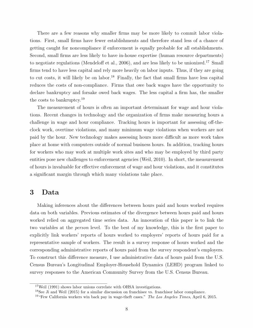
Figure 3 displays the distribution of log hours worked less log hours paid by LEHD hours
paid. I divide the annual hours paid measure from the LEHD by 52 weeks to obtain average
weekly hours paid. Figure 3 partitions the log difference distribution into those who on
average were paid less than 40 hours per week (top panel), 40 hours per week (middle panel),
and more than 40 hours per week (bottom panel). The top two panels show a significant
right skew in the distribution – what would be predicted from Figure 2. However, firms who
report paying for over 40 hours per week on average have a more symmetric distribution
with a mean of −0.020 [1.18]. In general, Figure 3 reinforces the finding that hours worked
and hours paid accord quite closely, but that hours worked over 40 hours per week are not
well recorded by employers.
The distributions of log hours worked less log hours paid suggest that hours worked is
accurately reported except for workers who report working more than 40 hours per week.
Recent studies support this finding by comparing survey responses from the Current Popu-
lation Survey (CPS) to the American Time Use Survey (ATUS). The ATUS is a time use
survey, and it is generally thought to more accurately reflect hours worked due to its short
33For comparison, Figure A.1 in appendix D shows the earnings error for the same two groups. Here, thedistributions show a significant left skew, but in general they are quite similar.
15

Figure 2: Distribution of the Difference of Log Hours Worked and Log Hours Paid by ACSusual weekly hours
Notes: Variable is the difference in log ACS hours worked from log LEHD hours paid for the full sample,winsorized at the 5% and 95% level. The variable is partitioned by whether an ACS respondent answersthat she usually works either 1) less than 40 hours per week (top panel) or 2) exactly 40 hours per week(middle panel) or 3) more than 40 hours per week (bottom panel). Top panel N = 49, 000, middle panelN = 108, 000, bottom panel N = 61, 000. Mean of top panel 0.031 [0.268], middle panel 0.032 [0.179] andbottom panel 0.21 [0.238].
16

Figure 3: Distribution of the Difference of Log Hours Worked and Log Hours Paid by LEHDHours Paid
Notes: Variable is the difference in log ACS hours worked from log LEHD hours paid for the full sample,winsorized at the 5% and 95% level. The variable is partitioned by average weekly hours paid (annualLEHD hours divided by 52). Top panel: less than 40 hours per week. Middle panel: exactly 40 hours aweek. Bottom panel: more than 40 hours per week. Top panel N = 116, 000, middle panel N = 24, 000,bottom panel N = 79, 000. Mean of bottom panel 0.158 [1.91], middle panel 0.108 [1.09] and bottom panel−0.020 [1.18].
17
recall period. Frazis and Stewart (2009) compare hours worked per job in the two surveys
at the person level. They find that survey responses from the CPS of hours worked are
remarkably close to the ATUS, with any overstatement confined to multiple jobholders.34
The conclusion of these validation studies is that respondents report work hours accurately
in surveys.
4 Hours & the Business Cycle
4.1 Empirical Strategy
Differentiating between the hypothesis of extra effort from employees in the form of off
the clock work when labor markets are slack versus the competing labor hoarding hypothesis
is the key empirical question. The ideal design for such an analysis would randomly assign
different unemployment rates, or other measures of labor market slack, to many identical
self-contained economies and then observe the co-movement of hours paid and hours worked.
Such a fantasy experiment is not feasible. This paper uses variation in local labor market
slack to infer the relationship between the business cycle and the difference between hours
paid and hours worked. Specifically, I use the variation in the change in unemployment rates
in commuting zones to identify hours off the clock. This approach takes advantage of the
large geographic dispersion of the United States, which effectively partitions the country into
many self-contained regional economies.35
I use the ACS respondent’s place of residence for the local labor market defined as a
commuting zone. Given the relatively small geographic area of four states and their adjoining
neighbors, I use commuting zones as the primary local labor market unit as it classifies
all counties into a commuting zone. The metropolitan statistical area (MSA) is also an
appealing geographic delineation for a local labor market as it is defined as a collection of
counties around a major (or minor) city usually including its suburbs. However, the MSA
excludes some mostly-rural counties from any MSA, which leads to further reductions in
sample size.36
I use the unemployment rate to measure the local labor market from the Local Area
Unemployment Statistics (LAUS) from the Bureau of Labor Statistics (BLS). LAUS provides
local area unemployment rates derived from BLS surveys and unemployment insurance data.
The data are available monthly for small areas including MSAs and counties. I use county
unemployment rates to construct monthly commuting zone unemployment rates by averaging
34See Frazis and Stewart (2010) and Frazis and Stewart (2004) for similar results.35Schaller (2016) is a recent example who employs a similar approach.36Headline results are robust to to local labor markets defined by MSA.
18
county unemployment rates for each county in a commuting zone weighting the average by
the labor force of each county. I then average monthly commuting zone unemployment
rates into a quarterly commuting zone unemployment rate. I use the quarterly commuting
zone unemployment rate corresponding to the quarter of the ACS survey response as an
indicator of labor market conditions. The LAUS unemployment rates are known to be noisy.
By averaging over the months in the reference quarter, I allow the data to accord to the
underlying analysis sample, and eliminate some of the noise.
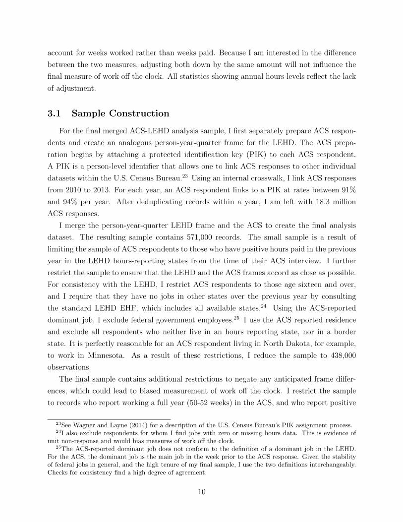
Figure 4 shows the time series of quarterly unemployment rates for the two largest com-
muting zones by population in the analysis sample. One commuting zone contains Min-
neapolis, Minnesota and the other contains Seattle, Washington. The unemployment rates
for both commuting zones rise quickly at the onset of the Great Recession before gradually
declining. Seattle’s commuting zone increases to almost 10% at its peak before declining to
below 7% at the end of the analysis sample. Minneapolis’s unemployment rate peaks at over
7% before 2010, and then declines to slightly below 5% at the end of 2013. For comparison,
the national unemployment rate declined from 9.8% in January 2010 to 6.6% in January
2014. All results that follow should be interpreted with these general macroeconomic con-
ditions in mind. Although this is just two commuting zones, Figure 4 shows that there is
ample variation both within and across commuting zones in the unemployment rate.37
The specification for the ordinary least squares (OLS) estimate is given by,
y52i,t = βUcz,t + δXi + ψJj(i) + αs + ωt + φcz + εi,t,cz . (2)
where y52i,t is the difference between the logarithm of ACS annual hours worked and the
logarithm of annual LEHD hours paid. I use my preferred 52-week measure for ACS hours
worked in the dependent variable. For this linear specification, the choice of dependent
variable corresponding to different weeks worked will not matter for the final estimates.
Differences in the dependent variable due to varying weeks worked only shift the intercept of
the regression line and have no effect on the slope, and therefore the coefficient of interest.
The variable Ucz,t is the unemployment rate in the commuting zone of the residence
of person i in interview quarter t. The vector Xi captures demographic characteristics of
person i, while Jj(i) captures job and firm characteristics of person i employed at dominant
job j. Job characteristics include tenure, industry fixed effects and an indicator variable for
whether a worker is employed in a supervisory or non-production occupation.38
37Figure A.3 shows the full distribution of unemployment rate changes across all commuting zones in theanalysis sample.
38I use the BLS definition for production and non-supervisory workers, which is defined by industry andoccupation. See U.S. Bureau of Labor Statistics (2004) for a detailed description.
19
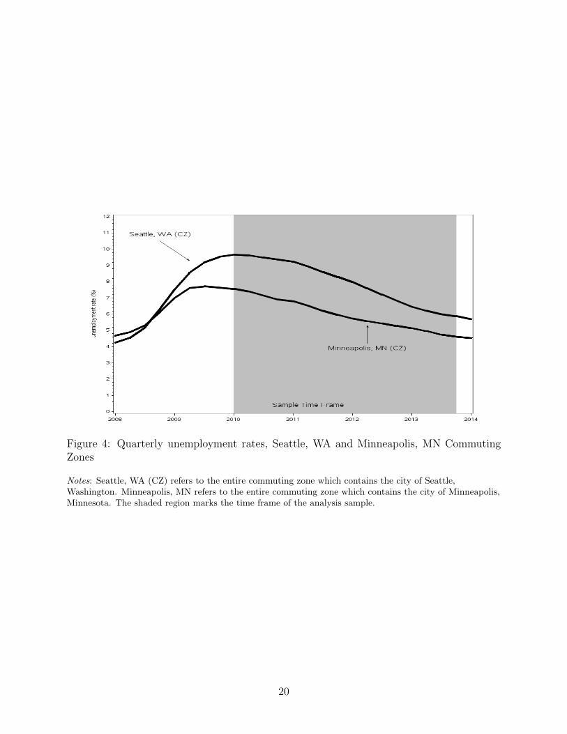
Figure 4: Quarterly unemployment rates, Seattle, WA and Minneapolis, MN CommutingZones
Notes: Seattle, WA (CZ) refers to the entire commuting zone which contains the city of Seattle,Washington. Minneapolis, MN refers to the entire commuting zone which contains the city of Minneapolis,Minnesota. The shaded region marks the time frame of the analysis sample.
20
I also include fixed commuting zone effects. Denoted φcz, the inclusion of fixed commuting
zone effects identifies the effect of the unemployment rate on the difference of log hours
using time-series variation within commuting zones. The inclusion of commuting zone time
trends in some specifications identifies the effect using de-trended time series variation within
commuting zones. I include additional controls for fixed year-quarter and state fixed effects
in the specification denoted ωt and αs, respectively. Finally, εi,t,cz is the error term.
Although commonly used in the literature, the use of local unemployment rates presents
some problems for measures of labor market slack. The unemployment rate confounds both
supply and demand induced responses of labor force participation. Changes in the unem-
ployment rate may be endogenous to other variables forcing changes in work off the clock.
In this setting, where the dependent variable is the difference in log hours worked from log
hours paid, such endogenous changes are harder to envision, but it is not implausible that
changes in state or local labor programs to encourage labor force participation may also
change an employer’s unemployment insurance hours reporting requirements.39
In order to buttress the results using the local unemployment rate, I also construct an
employment shift-share measure of plausibly exogenous labor demand. This shift-share index
commonly credited to Bartik (1991), but used extensively in local labor market analyses,40
uses a local labor market’s industrial composition in a base year to predict employment
growth in the local labor market in subsequent years. The intuition behind the instrument
is to fix local industrial composition, and allow national employment growth to predict local
employment growth. If drivers of national growth are applied uniformly, local labor markets
with greater concentrations of the growth industries should see greater predicted employment
growth simply due to their industrial composition. I follow Autor and Duggan (2003) and
construct predicted employment growth in labor market cz at time t from base year t0 as
Gt,cz =∑k
δt0,cz,kGt,k .
The first term, δt0,cz,k, gives the share of employment in NAICS sector k in local labor market
cz at time t0, and the second term, Gt,k, is the change in log national employment in NAICS
sector k between the base year and time t. I exclude the local labor market cz for the
computation of national growth rates for each local labor market.41
39It appears Rhode Island began requiring employers to report hours paid at the same time it began anew labor market policy. Whether the former is in response to the latter has proven difficult to pin down.
40See Blanchard and Katz (1991) Bound and Holzer (2000) Autor and Duggan (2003) for other examples.41National employment growth rates are from the Bureau of Labor Statistics CEW, and I construct local
labor market shares from the U.S. Census Bureau’s QWI, which is benchmarked to the CEW. I use 2007 forthe base year because it is the peak of previous business cycle, though results are robust to using year 2000.
21
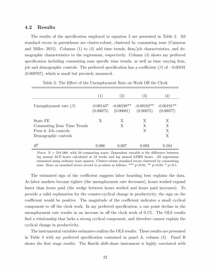
4.2 Results
The results of the specification employed in equation 2 are presented in Table 2. All
standard errors in parentheses are cluster-robust, clustered by commuting zone (Cameron
and Miller, 2015). Columns (1) to (4) add time trends, firm/job characteristics, and de-
mographic characteristics to the regressions, respectively. Column (4) shows my preferred
specification including commuting zone specific time trends, as well as time varying firm,
job and demographic controls. The preferred specification has a coefficient (β) of −0.00191
(0.000767), which is small but precisely measured.
Table 2: The Effect of the Unemployment Rate on Work Off the Clock
(1) (2) (3) (4)
Unemployment rate (β) -0.00143* -0.00198** -0.00182** -0.00191**(0.00075) (0.00081) (0.00075) (0.00077)
State FE X X X XCommuting Zone Time Trends X X XFirm & Job controls X XDemographic controls X
R2 0.006 0.007 0.093 0.104
Notes: N = 218, 000, with 58 commuting zones. Dependent variable is the difference betweenlog annual ACS hours calculated at 52 weeks and log annual LEHD hours. All regressionsestimated using ordinary least squares. Cluster-robust standard errors clustered by commutingzone. Stars on standard errors accord to p-values as follows: *** p<0.01, ** p<0.05, * p<0.1.
The estimated sign of the coefficient suggests labor hoarding best explains the data.
As labor markets become tighter (the unemployment rate decreases), hours worked expand
faster than hours paid (the wedge between hours worked and hours paid increases). To
provide a valid explanation for the counter-cyclical change in productivity, the sign on the
coefficient would be positive. The magnitude of the coefficient indicates a small cyclical
component to off the clock work. In my preferred specification, a one point decline in the
unemployment rate results in an increase in off the clock work of 0.1%. The OLS results
find a relationship that lacks a strong cyclical component, and therefore cannot explain the
cyclical change in productivity.
The instrumental variables estimates confirm the OLS results. These results are presented
in Table 3 with my preferred specification contained in panel A, column (3). Panel B
shows the first stage results. The Bartik shift-share instrument is highly correlated with
22

Table 3: The Effect of the Unemployment Rate on Work Off theClock, Two Stage Least Squares Results
(1) (2) (3)
Panel A: 2SLS Results
Unemployment rate (β) -0.00286 -0.00254 -0.00274*(0.00177) (0.00159) (0.00154)
Panel B: First Stage Results
Bartik Shift-Share -29.07*** -27.78*** -27.80***(3.790) (3.987) (3.994)
First stage F -Statistic 58.84 48.57 48.43
State FE X X XCommuting Zone Time Trends X XFirm & Job controls XDemographic controls XR2 0.005 0.006 0.104
Notes: N = 218, 000, with 58 commuting zones. Dependent variable is thedifference between log annual ACS hours calculated at 52 weeks and log annualLEHD hours. Panel A shows two stage least squares estimates. Panel Bshows the corresponding first stage regressions. Cluster-robust standard errorsclustered by commuting zone. Stars on standard errors accord to p-values asfollows: *** p<0.01, ** p<0.05, * p<0.1.
23
the unemployment rate across all specifications. The coefficient on predicted employment
growth is −27.8 (3.99), with the sign in the correct direction (higher predicted employment
growth leads to a lower unemployment rate), and a first stage F -statistic of 48.43. The
two stage least squares coefficient on the unemployment rate in column (3) is still negative
and larger in absolute value than in the OLS specification in column (2). The coefficient
on unemployment is now −0.00274 (0.00154). The instrumental variables estimates come
with the cost of a loss in precision with the coefficient only significant at the 10% level.
The instrumental variables results provide evidence for supply-induced responses possibly
attenuating the OLS results.
The headline results of a limited cyclical component mask heterogeneity in off the clock
work and the business cycle. Table 4 fits the same model given in equation 2, but interacts the
unemployment rate with subgroups most likely to work off the clock.42 Column (1) shows
the slopes of the regression lines associated with production and non-supervisory workers
and their complement, supervisory workers. Supervisory workers are most likely to be paid
a fixed salary and seem likely candidates to be driving off the clock work.43 Somewhat
surprisingly, column (1) shows that it is production and non-supervisory workers driving the
results. The coefficient estimate is −0.00219 (0.00075). In contrast, the estimate for the
coefficient for supervisory workers is imprecise and slightly positive, 0.00111 (0.00080).
Similar results obtain when interacting the unemployment rate by method of pay and by
skill level. Column (3) in Table 4 interacts the results by whether the ACS respondent is
likely paid by the hour. Workers most unlikely to be paid hourly have a coefficient on the
slope of the regression line of 0.00049 (0.00091). In contrast, workers most likely be paid
by the hour have an estimated coefficient of −0.00214 (0.000852). Column (2) shows the
results for workers with and without a bachelor’s degree. Although there is no a priori reason
why workers with a bachelor’s degree would be more or less likely to work off the clock, in
practice a bachelor’s degree is highly correlated with supervisory work and non-hourly pay
arrangements. The point estimate for workers without a bachelors degree is qualitatively
similar to the coefficient on non-supervisory workers, and precise, obtaining an estimate of
−0.00220 (0.00079). The results confirm that it is lower skilled workers likely paid by the
hour who are driving the results.
The preceding results show support for labor hoarding driving the cyclical component
of off the clock work, though the effect is small. Another further confirmation of the labor
hoarding hypothesis is the tenure of workers. Firms holding onto excess labor in a downturn
42Table A.5 shows qualitatively similar results by running the regression separately for each group.43This is due to the duties test for exemption from overtime in the FLSA. A key component of the test
is whether an employee works in a supervisory capacity.
24
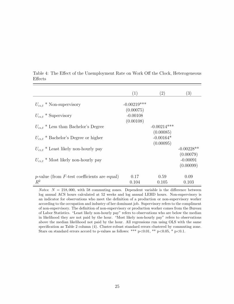
Table 4: The Effect of the Unemployment Rate on Work Off the Clock, HeterogeneousEffects
(1) (2) (3)
Ucz,t * Non-supervisory -0.00219***(0.00075)
Ucz,t * Supervisory -0.00108(0.00108)
Ucz,t * Less than Bachelor’s Degree -0.00214***(0.00085)
Ucz,t * Bachelor’s Degree or higher -0.00164*(0.00095)
Ucz,t * Least likely non-hourly pay -0.00228**(0.00079)
Ucz,t * Most likely non-hourly pay -0.00091(0.00099)
p-value (from F -test coefficients are equal) 0.17 0.59 0.09R2 0.104 0.105 0.103
Notes: N = 218, 000, with 58 commuting zones. Dependent variable is the difference betweenlog annual ACS hours calculated at 52 weeks and log annual LEHD hours. Non-supervisory isan indicator for observations who meet the definition of a production or non-supervisory workeraccording to the occupation and industry of her dominant job. Supervisory refers to the complimentof non-supervisory. The definition of non-supervisory or production worker comes from the Bureauof Labor Statistics. “Least likely non-hourly pay” refers to observations who are below the medianin likelihood they are not paid by the hour. “Most likely non-hourly pay” refers to observationsabove the median likelihood not paid by the hour. All regressions run using OLS with the samespecification as Table 2 column (4). Cluster-robust standard errors clustered by commuting zone.Stars on standard errors accord to p-values as follows: *** p<0.01, ** p<0.05, * p<0.1.
25

will be eager to deploy it once demand picks up. In contrast, in an efficiency wage setting
it seems plausible that workers with strong attachment to particular jobs who also happen
to retain their dominant job after the Great Recession are particularly good matches with
their employers, and their high tenure precludes them from feeling threatened with layoffs.44
Table 5 shows the results interacting various firm and job characteristics with the local
unemployment rate. Column (1) gives the results for tenure, where the estimating equation
augments equation 2 with indicator variables for length of tenure one year or less, 1-3 years,
3-5 years, and greater than 5 years. The estimated slopes show that it is longer tenured
workers driving the results with point estimates of −0.00230 (0.00786), −0.00223 (0.00803),
and −0.00170 (0.00754), for workers with 1-3 years, 3-5 years, and greater than 5 years
of tenure, respectively. These coefficient estimates are all significant, and much larger in
magnitude than for workers who have less than one year of tenure. Table 5 also shows that
off the clock work is concentrated in large, old firms. The results suggest a labor hoarding
model where firms work the excess labor they have kept during a downturn harder during
the ensuing recovery.45 The results further suggest that although likely paid a salary, higher
skill workers likely have better outside options and are better able to resist pressures to vary
hours according to cyclical labor market pressure.
4.3 Robustness Checks
The first robustness check tests for sensitivity of the results to the specification of the
dependent variable. The first two columns of Table 6 run regression 2 using alternate spec-
ifications of work off the clock. Column (1) shows the results using the disparity between
hours worked and hours paid according to Tornqvist et al. (1985).46 This measure is defined
if either hours measure is equal to zero, and is roughly equivalent to the log measure of the
percent difference. I also do not winsorize this variable. Column (2) uses a binary indicator
variable for the dependent variable, which equals unity if hours worked in the ACS exceeds
hours paid from the LEHD. This makes equation 2 a linear probability model. The point
estimates on the unemployment rate for columns (1) and (2) are −0.00183 (0.00080) and
−0.00505 (0.00204), respectively. The estimates are precise, and indicate that the results
are not sensitive to the specification of the dependent variable.
44This is one result of the model of Rebitzer (1987).45Table A.6 shows the correlation between off the clock work and firm employment growth. There is little
correlation. This is not inconsistent with a model of firms with large fixed adjustment costs who work theirexisting workforce as long and hard as possible before eventually adjusting.
46Formally, this is yalti =Hi,acs−Hi,lehd
12 (Hi,acs+Hi,lehd)
. Within the economics literature, this measure is usually
credited to Haltiwanger et al. (1996).
26
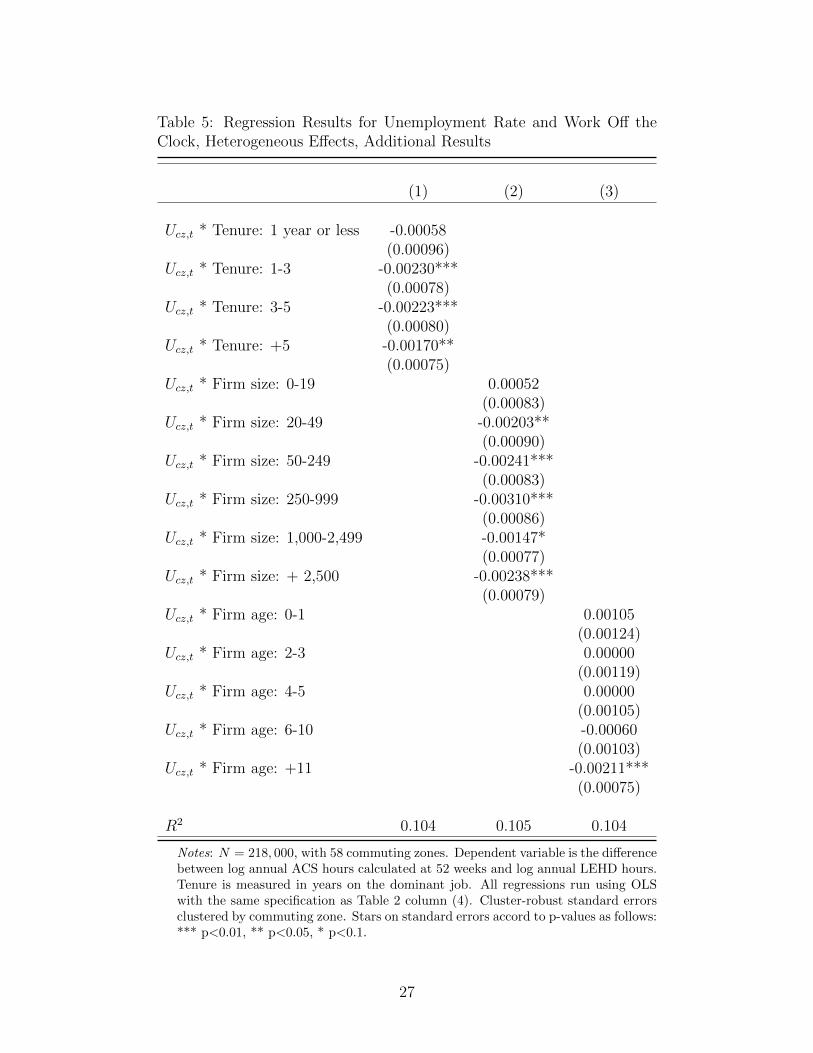
Table 5: Regression Results for Unemployment Rate and Work Off theClock, Heterogeneous Effects, Additional Results
(1) (2) (3)
Ucz,t * Tenure: 1 year or less -0.00058(0.00096)
Ucz,t * Tenure: 1-3 -0.00230***(0.00078)
Ucz,t * Tenure: 3-5 -0.00223***(0.00080)
Ucz,t * Tenure: +5 -0.00170**(0.00075)
Ucz,t * Firm size: 0-19 0.00052(0.00083)
Ucz,t * Firm size: 20-49 -0.00203**(0.00090)
Ucz,t * Firm size: 50-249 -0.00241***(0.00083)
Ucz,t * Firm size: 250-999 -0.00310***(0.00086)
Ucz,t * Firm size: 1,000-2,499 -0.00147*(0.00077)
Ucz,t * Firm size: + 2,500 -0.00238***(0.00079)
Ucz,t * Firm age: 0-1 0.00105(0.00124)
Ucz,t * Firm age: 2-3 0.00000(0.00119)
Ucz,t * Firm age: 4-5 0.00000(0.00105)
Ucz,t * Firm age: 6-10 -0.00060(0.00103)
Ucz,t * Firm age: +11 -0.00211***(0.00075)
R2 0.104 0.105 0.104
Notes: N = 218, 000, with 58 commuting zones. Dependent variable is the differencebetween log annual ACS hours calculated at 52 weeks and log annual LEHD hours.Tenure is measured in years on the dominant job. All regressions run using OLSwith the same specification as Table 2 column (4). Cluster-robust standard errorsclustered by commuting zone. Stars on standard errors accord to p-values as follows:*** p<0.01, ** p<0.05, * p<0.1.
27
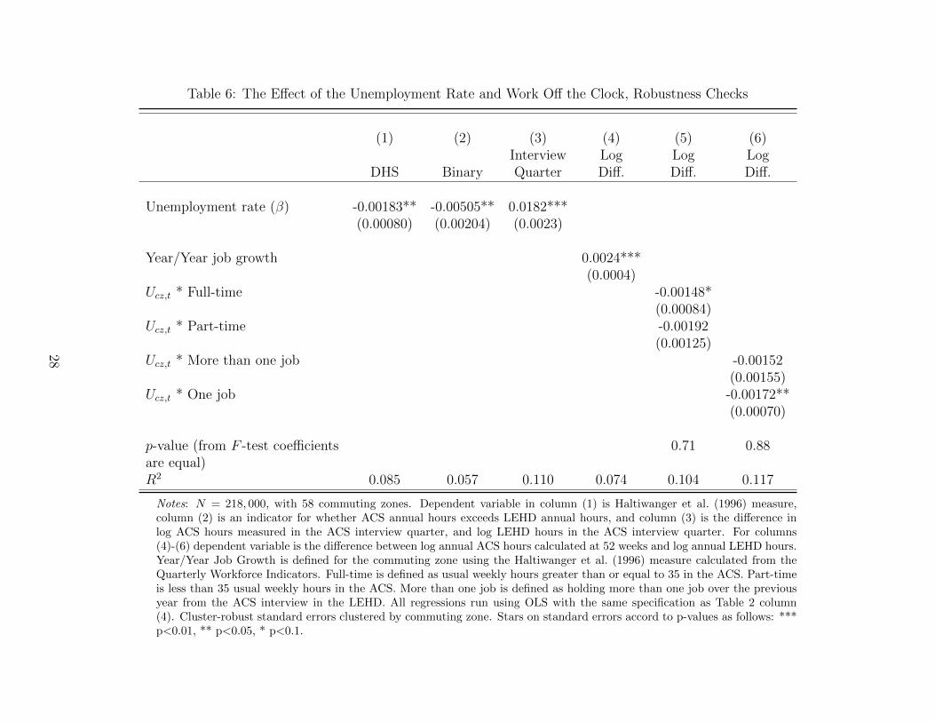
Table 6: The Effect of the Unemployment Rate and Work Off the Clock, Robustness Checks
(1) (2) (3) (4) (5) (6)Interview Log Log Log
DHS Binary Quarter Diff. Diff. Diff.
Unemployment rate (β) -0.00183** -0.00505** 0.0182***(0.00080) (0.00204) (0.0023)
Year/Year job growth 0.0024***(0.0004)
Ucz,t * Full-time -0.00148*(0.00084)
Ucz,t * Part-time -0.00192(0.00125)
Ucz,t * More than one job -0.00152(0.00155)
Ucz,t * One job -0.00172**(0.00070)
p-value (from F -test coefficients 0.71 0.88are equal)R2 0.085 0.057 0.110 0.074 0.104 0.117
Notes: N = 218, 000, with 58 commuting zones. Dependent variable in column (1) is Haltiwanger et al. (1996) measure,column (2) is an indicator for whether ACS annual hours exceeds LEHD annual hours, and column (3) is the difference inlog ACS hours measured in the ACS interview quarter, and log LEHD hours in the ACS interview quarter. For columns(4)-(6) dependent variable is the difference between log annual ACS hours calculated at 52 weeks and log annual LEHD hours.Year/Year Job Growth is defined for the commuting zone using the Haltiwanger et al. (1996) measure calculated from theQuarterly Workforce Indicators. Full-time is defined as usual weekly hours greater than or equal to 35 in the ACS. Part-timeis less than 35 usual weekly hours in the ACS. More than one job is defined as holding more than one job over the previousyear from the ACS interview in the LEHD. All regressions run using OLS with the same specification as Table 2 column(4). Cluster-robust standard errors clustered by commuting zone. Stars on standard errors accord to p-values as follows: ***p<0.01, ** p<0.05, * p<0.1.
28
The next threat to identification comes from recall bias. The ACS asks the respondent for
usual weekly hours over the previous year. My measure of work off the clock assumes “usual”
weekly hours is equivalent to average weekly hours, to respondents.47 Hours are growing in
the analysis sample as the unemployment rate trends down between 2010 and 2013. It is
possible that workers simply report their usual hours right around the time of interview, and
not over the previous year. If this is the case, then my results will show a positive relationship
between work off the clock and tightening of the local labor market – exactly what I find.
To test for this, in column (3) of Table 6 I use the difference between log hours worked and
log hours paid in the interview quarter.48 If ACS respondents understand usual hours to
mean hours over the previous year, this new measure should yield a positive coefficient –
the average over the previous year will be smaller than the interview quarter. If respondents
are giving usual hours in the interview quarter, the point estimate on the unemployment
rate should be close to zero and/or imprecisely measured. The positive estimate in column
(3) of 0.0182 (0.0023), suggests that respondents interpret usual weekly hours as asking for
average hours in the analysis time frame.
Table 6, column (4) tests whether the results are sensitive to the measure of labor market
slack. The Local Area Unemployment Statistics from the BLS are model based, and known
to be noisy. In column (3) I use the year-over-year job growth rate for the commuting zone
calculated using the approximate log change credited to Haltiwanger et al. (1996). The year
over year growth rate is measured from one year prior to the interview quarter. The data
come from the Quarterly Workforce Indicators (QWI) from the U.S. Census Bureau. The
QWI are the public-use version of the LEHD, and are therefore derived from administrative
unemployment insurance data. The coefficient estimate using the year over year job growth
rate is 0.0024 (0.0041). The estimate is precise and the sign of the coefficient is in the correct
direction. That is, a positive coefficient for local employment growth is consistent with a
negative coefficient for the local unemployment rate.49
Another potential problem with my specification is that some jobs may not be reported
to the unemployment insurance system at all. If the ACS respondent includes the hours from
these jobs in usual weekly hours, this could bias the results to look like labor hoarding.50 The
47The exact question is (capitalization as in original), “During the PAST 12 MONTHS, in the WEEKSWORKED, how many hours did this person usually work each WEEK?”
48I use the log of gross hours in the interview quarter for hours paid and the log of usual weekly hoursscaled by the number of weeks in the quarter for hours worked.
49Results are robust to sensitivity of included commuting zones, and the later inclusion of Oregon in 2012,though with a loss of precision in the latter case. Due to disclosure risks, these results are not able to bereleased at this time.
50From the perspective of a statistical agency calculating productivity, this distinction between “off thebooks” and “off the clock” is likely irrelevant.
29
construction of the analysis sample makes this scenario unlikely, but I test for off the books
work by interacting the unemployment rate by full time status and multiple job holding.51
The assumption is that workers who hold multiple jobs and/or work part-time are more
likely to pick up short, informal jobs that are not reported to the unemployment insurance
system. The results are given in columns (5) and (6) of Table 6. The coefficients for the
slope of part-time workers and multiple job holders are 0.00044 (0.001199) and −0.00155
(0.00154), respectively. Neither estimate is precise, though the coefficient on multiple job
holders suggests that it is not implausible off the books work may be influencing the results.
5 Hours & Labor Compliance
5.1 Empirical Strategy
Somewhat surprisingly, this paper finds that off the clock work has a small pro-cyclical
component, which is driven by low-skill workers likely paid by the hour. Non-compliance
with labor market regulations offers a possible explanation for these results. Non-compliance
can either be explicit, by paying workers under the table, or refusing to pay over-time for
hours worked over 40 hours per week. There are also subtle ways this can arise. For example
firms may mis-classify employees who should be non-exempt as exempt, and shift more
hours to these workers. To test this theory, we need to use the characteristics of firms. In
particular, theory and survey evidence suggest that small firms are more likely to engage in
non-compliance behavior due to lower costs of bankruptcy, diminished reputation, and lower
productivity firms.52
The relevant facts presented in Section 2 indicate that off-the-clock work, and wage
and hour violations often times operate through the (mis)management of hours of work.
Even in the case of minimum wage violations, non-hourly pay frequency and its associated
ambiguity of work hours is correlated with FLSA violations. In this section I test for whether
hours-based evidence for work off the clock is present in my representative microdata. I use
ordinary least squares regression and follow the specification of Bernhardt et al. (2013) using
survey data, as well as Ji and Weil (2015) who use administrative data.
Before analyzing firm characteristics in greater depth, I study the following specification
in order to ensure that key variables behave roughly as expected. The model is,
y52i,t = δXi + ψJj(i) + αs + ωt + εi,t,cz , (3)
51I calculate multiple job holding summing the number of jobs in the LEHD over the previous year.52Milkman et al. (2012) and Mendeloff et al. (2006) provide recent examples.
30
where the vector Xi captures demographic characteristics of person i, while Jj(i) captures job
and firm characteristics of person i employed at dominant job j. The specification is close to
equation 2, except for the omission of commuting zone effects. The empirical strategy used
to identify off the clock work for labor compliance does not rely on variation in local labor
market conditions. I therefore drop the commuting zone effects as well as commuting zone
time trends.
In addition to the standard firm and individual controls, I augment the model with
indicators for firm size. Both Bernhardt et al. (2013) and Ji and Weil (2015) emphasize the
role played by firm size in labor violations. I therefore augment equation 3 vector Jj(i) with
bins for firm size given by,
B∑b=1
ψb1{kb ≤ firmsizej(i) < kb+1} ,
where b indexes the bins with B total bins, and k is the set of bounds defining the bins with
B+1 bounds. The indicator function takes a value of one if firmsizej(i) – the firm size of the
LEHD dominant job – falls within the specified firm size category. The firm-person match
which constitutes a job in the LEHD uses a definition of a firm as a state-level tax reporting
entity. It is not uncommon for a larger national entity to be the real owner of a firm, with
the state distinction a product of the state-based nature of unemployment insurance records.
The LEHD remedies this by bringing in firm size from the U.S. Census Bureau’s Longitudinal
Business Database (LBD). All firm size categories use the LBD’s definition of a firm taking
into account inter-state ownership.
5.2 Results: Firm Size
The estimation results for equation 3 are given in Table 7. My preferred specification
given in column (1) lines up well with prior research. Workers with a bachelors degree,
men, and workers whose main job is with a private, for profit firm are more likely to report
more hours worked than hours paid. Two curious results are that the model indicates that
people of color report fewer hours worked than hours paid, and U.S. citizens slightly more
hours worked than hours paid. The higher incidence of work off the clock for U.S. citizens
is likely due to the fact that previous survey evidence included workers who are not able
to legally work in the U.S. The analysis sample includes only workers who are found in the
administrative data. Inclusion in the UI data generally necessitates a social security number
suggesting that non-citizens in the sample are likely different than non-citizens in purely
survey data. For workers of color, the difference in sign has no easy explanation, other than
31

previous results found only a tenuous relationship between race and labor compliance.
The coefficients of greatest interest are on the indicator variables for supervisory workers
and on the quartiles of likelihood a worker is not paid by the hour. It is generally assumed
that employers pay little attention to the hours for supervisory workers because they are
exempt from overtime and usually not paid by the hour. In such cases one should expect
hours worked to exceed hours paid. The coefficient on the indicator for supervisory workers in
the main specification in column (1) is 0.00909 (0.0050) indicating that supervisory workers,
all else equal, work 0.9% more hours than those for which they are paid over the course of
the year. At first glance this seems low, but it is important to realize that this indicator,
based on BLS definitions of supervisory workers, is highly correlated with my imputation of
non-hourly pay probability.
I measure non-hourly pay probability and its association with work off the clock by
indicators for quartiles of probability of non-hourly pay. In Table 7 column (1) the indicators
for quartile of non-hourly pay are measured relative to the lowest quartile, where workers
most are likely to be paid by the hour. The results indicate that workers most likely to
be in non-hourly pay arrangements are the most likely to report more hours worked than
hours paid. The coefficient in this case is 0.0136 (0.0059). Column (2) in the same table
fits equation 3 using OLS but subsets the data to only include those in the top quartile
of likelihood of non-hourly pay. Results are in general qualitatively unchanged, though the
coefficient on the indicator for supervisory flips sign – it is now negative – indicating the
limited explanatory power of this distinction in comparison to the pay type, although these
two effects are difficult to distinguish.
32

Table 7: Characteristics of Work Off the Clock: OLSResults
(1) (2)
Private, for-profit firm 0.0125*** 0.0135***(0.00281) (0.00497)
Not White -0.0270*** -0.0483***(0.00563) (0.00306)
Hispanic -0.00869* -0.00969(0.00522) (0.00624)
Male 0.00445** 0.00830***(0.00180) (0.00142)
U.S. Citizen 0.0319*** 0.0203***(0.00584) (0.00269)
Bachelors degree of higher 0.0486*** 0.0572***(0.00175) (0.00316)
Supervisory Worker 0.00909* -0.00970*(0.00502) (0.00566)
Second Quartile -0.0463***(0.00346)
Third Quartile -0.0355***(0.00538)
Top Quartile 0.0136**(0.00591)
Firm Controls X XYear-Quarter FE X XState FE X XDemographic Controls X X
Observations 218,000 67,000R2 0.073 0.096
Notes: Dependent variable is the difference between log an-nual ACS hours calculated at 52 weeks and log annual LEHDhours. Quartile is the quartile of likelihood paid non-hourly.Supervisory worker is defined by observation’s industry andoccupation according to BLS definition of production andnon-supervisory workers. Column (2) subsets the regressionto only observations in the top quartile of likely non-hourlypay. Cluster-robust standard errors clustered by state-firm.Stars on standard errors accord to p-values as follows: ***p<0.01, ** p<0.05, * p<0.1.
33
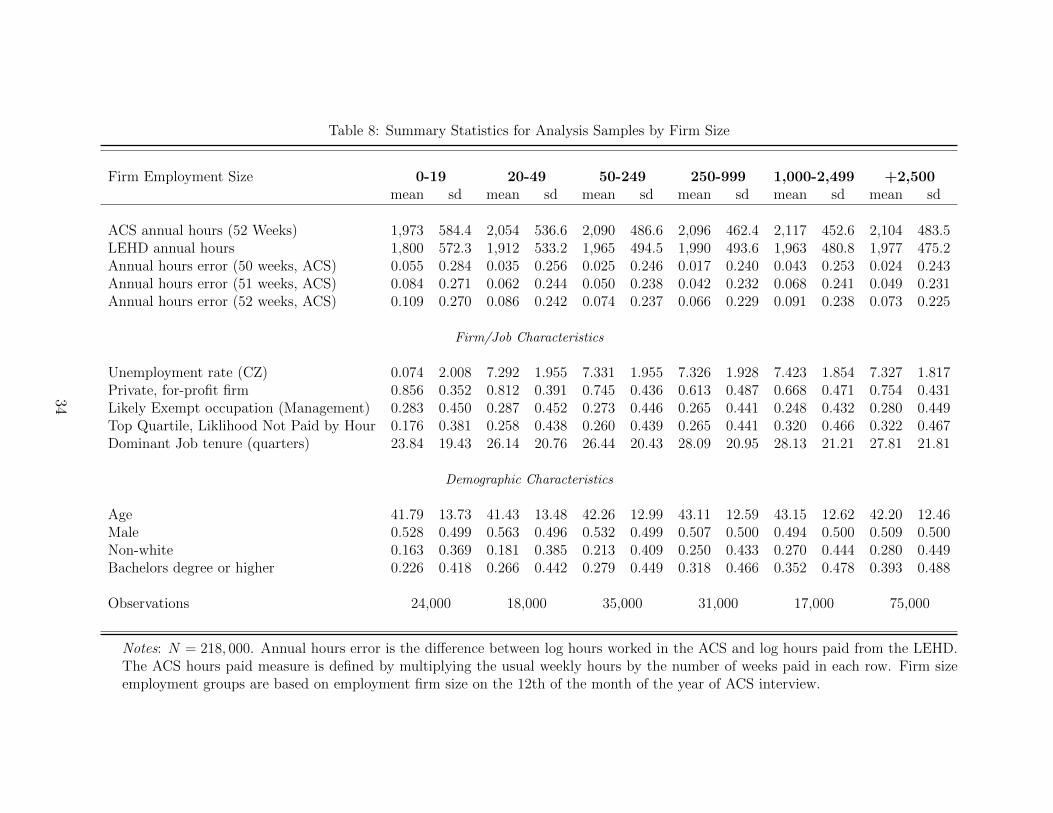
Table 8: Summary Statistics for Analysis Samples by Firm Size
Firm Employment Size 0-19 20-49 50-249 250-999 1,000-2,499 +2,500mean sd mean sd mean sd mean sd mean sd mean sd
ACS annual hours (52 Weeks) 1,973 584.4 2,054 536.6 2,090 486.6 2,096 462.4 2,117 452.6 2,104 483.5LEHD annual hours 1,800 572.3 1,912 533.2 1,965 494.5 1,990 493.6 1,963 480.8 1,977 475.2Annual hours error (50 weeks, ACS) 0.055 0.284 0.035 0.256 0.025 0.246 0.017 0.240 0.043 0.253 0.024 0.243Annual hours error (51 weeks, ACS) 0.084 0.271 0.062 0.244 0.050 0.238 0.042 0.232 0.068 0.241 0.049 0.231Annual hours error (52 weeks, ACS) 0.109 0.270 0.086 0.242 0.074 0.237 0.066 0.229 0.091 0.238 0.073 0.225
Firm/Job Characteristics
Unemployment rate (CZ) 0.074 2.008 7.292 1.955 7.331 1.955 7.326 1.928 7.423 1.854 7.327 1.817Private, for-profit firm 0.856 0.352 0.812 0.391 0.745 0.436 0.613 0.487 0.668 0.471 0.754 0.431Likely Exempt occupation (Management) 0.283 0.450 0.287 0.452 0.273 0.446 0.265 0.441 0.248 0.432 0.280 0.449Top Quartile, Liklihood Not Paid by Hour 0.176 0.381 0.258 0.438 0.260 0.439 0.265 0.441 0.320 0.466 0.322 0.467Dominant Job tenure (quarters) 23.84 19.43 26.14 20.76 26.44 20.43 28.09 20.95 28.13 21.21 27.81 21.81
Demographic Characteristics
Age 41.79 13.73 41.43 13.48 42.26 12.99 43.11 12.59 43.15 12.62 42.20 12.46Male 0.528 0.499 0.563 0.496 0.532 0.499 0.507 0.500 0.494 0.500 0.509 0.500Non-white 0.163 0.369 0.181 0.385 0.213 0.409 0.250 0.433 0.270 0.444 0.280 0.449Bachelors degree or higher 0.226 0.418 0.266 0.442 0.279 0.449 0.318 0.466 0.352 0.478 0.393 0.488
Observations 24,000 18,000 35,000 31,000 17,000 75,000
Notes: N = 218, 000. Annual hours error is the difference between log hours worked in the ACS and log hours paid from the LEHD.The ACS hours paid measure is defined by multiplying the usual weekly hours by the number of weeks paid in each row. Firm sizeemployment groups are based on employment firm size on the 12th of the month of the year of ACS interview.
34
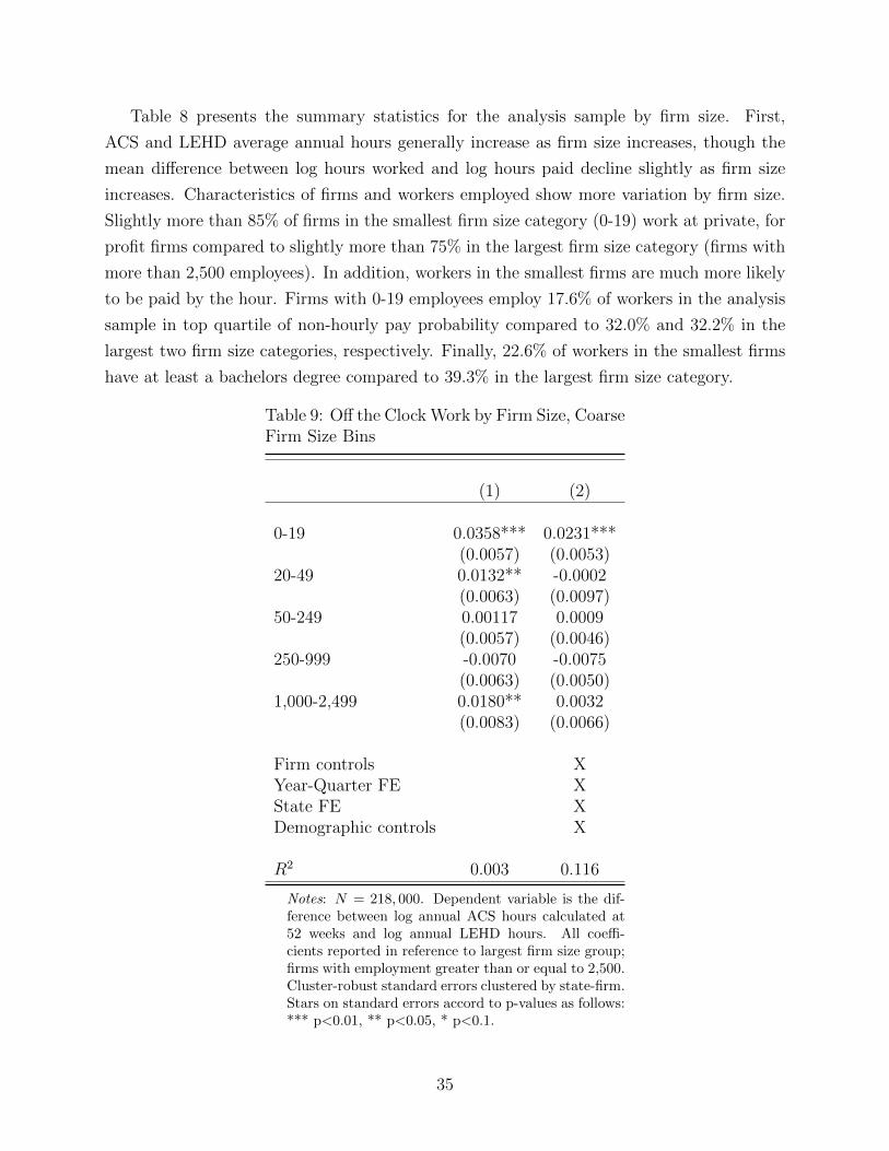
Table 8 presents the summary statistics for the analysis sample by firm size. First,
ACS and LEHD average annual hours generally increase as firm size increases, though the
mean difference between log hours worked and log hours paid decline slightly as firm size
increases. Characteristics of firms and workers employed show more variation by firm size.
Slightly more than 85% of firms in the smallest firm size category (0-19) work at private, for
profit firms compared to slightly more than 75% in the largest firm size category (firms with
more than 2,500 employees). In addition, workers in the smallest firms are much more likely
to be paid by the hour. Firms with 0-19 employees employ 17.6% of workers in the analysis
sample in top quartile of non-hourly pay probability compared to 32.0% and 32.2% in the
largest two firm size categories, respectively. Finally, 22.6% of workers in the smallest firms
have at least a bachelors degree compared to 39.3% in the largest firm size category.
Table 9: Off the Clock Work by Firm Size, CoarseFirm Size Bins
(1) (2)
0-19 0.0358*** 0.0231***(0.0057) (0.0053)
20-49 0.0132** -0.0002(0.0063) (0.0097)
50-249 0.00117 0.0009(0.0057) (0.0046)
250-999 -0.0070 -0.0075(0.0063) (0.0050)
1,000-2,499 0.0180** 0.0032(0.0083) (0.0066)
Firm controls XYear-Quarter FE XState FE XDemographic controls X
R2 0.003 0.116
Notes: N = 218, 000. Dependent variable is the dif-ference between log annual ACS hours calculated at52 weeks and log annual LEHD hours. All coeffi-cients reported in reference to largest firm size group;firms with employment greater than or equal to 2,500.Cluster-robust standard errors clustered by state-firm.Stars on standard errors accord to p-values as follows:*** p<0.01, ** p<0.05, * p<0.1.
35
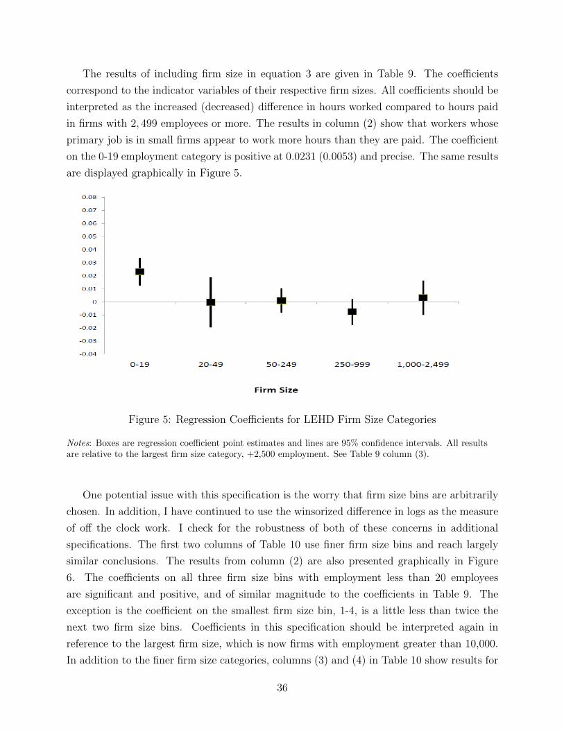
The results of including firm size in equation 3 are given in Table 9. The coefficients
correspond to the indicator variables of their respective firm sizes. All coefficients should be
interpreted as the increased (decreased) difference in hours worked compared to hours paid
in firms with 2, 499 employees or more. The results in column (2) show that workers whose
primary job is in small firms appear to work more hours than they are paid. The coefficient
on the 0-19 employment category is positive at 0.0231 (0.0053) and precise. The same results
are displayed graphically in Figure 5.
Figure 5: Regression Coefficients for LEHD Firm Size Categories
Notes: Boxes are regression coefficient point estimates and lines are 95% confidence intervals. All resultsare relative to the largest firm size category, +2,500 employment. See Table 9 column (3).
One potential issue with this specification is the worry that firm size bins are arbitrarily
chosen. In addition, I have continued to use the winsorized difference in logs as the measure
of off the clock work. I check for the robustness of both of these concerns in additional
specifications. The first two columns of Table 10 use finer firm size bins and reach largely
similar conclusions. The results from column (2) are also presented graphically in Figure
6. The coefficients on all three firm size bins with employment less than 20 employees
are significant and positive, and of similar magnitude to the coefficients in Table 9. The
exception is the coefficient on the smallest firm size bin, 1-4, is a little less than twice the
next two firm size bins. Coefficients in this specification should be interpreted again in
reference to the largest firm size, which is now firms with employment greater than 10,000.
In addition to the finer firm size categories, columns (3) and (4) in Table 10 show results for
36
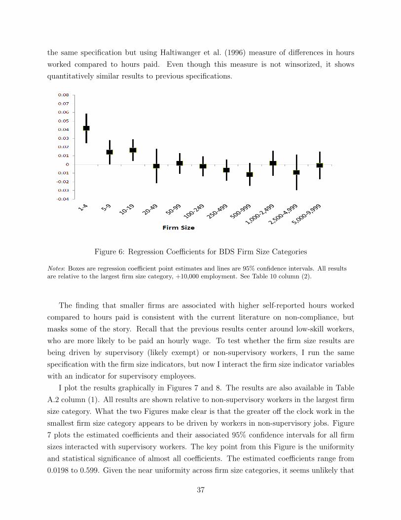
the same specification but using Haltiwanger et al. (1996) measure of differences in hours
worked compared to hours paid. Even though this measure is not winsorized, it shows
quantitatively similar results to previous specifications.
Figure 6: Regression Coefficients for BDS Firm Size Categories
Notes: Boxes are regression coefficient point estimates and lines are 95% confidence intervals. All resultsare relative to the largest firm size category, +10,000 employment. See Table 10 column (2).
The finding that smaller firms are associated with higher self-reported hours worked
compared to hours paid is consistent with the current literature on non-compliance, but
masks some of the story. Recall that the previous results center around low-skill workers,
who are more likely to be paid an hourly wage. To test whether the firm size results are
being driven by supervisory (likely exempt) or non-supervisory workers, I run the same
specification with the firm size indicators, but now I interact the firm size indicator variables
with an indicator for supervisory employees.
I plot the results graphically in Figures 7 and 8. The results are also available in Table
A.2 column (1). All results are shown relative to non-supervisory workers in the largest firm
size category. What the two Figures make clear is that the greater off the clock work in the
smallest firm size category appears to be driven by workers in non-supervisory jobs. Figure
7 plots the estimated coefficients and their associated 95% confidence intervals for all firm
sizes interacted with supervisory workers. The key point from this Figure is the uniformity
and statistical significance of almost all coefficients. The estimated coefficients range from
0.0198 to 0.599. Given the near uniformity across firm size categories, it seems unlikely that
37

Table 10: Off the Clock Work by Firm Size, Fine Firm Size Bins
(1) (2) (3) (4)
1-4 0.0586*** 0.0418*** 0.0505*** 0.0425***(0.0096) (0.0086) (0.0106) (0.0095)
5-9 0.0302*** 0.0142** 0.0295*** 0.0205**(0.0080) (0.0070) (0.0093) (0.0081)
10-19 0.0241*** 0.0164*** 0.0250*** 0.0228***(0.0078) (0.0063) (0.0092) (0.0074)
20-49 0.0119 -0.0018 0.0125 0.00247(0.0081) (0.0101) (0.0095) (0.0110)
50-99 0.00165 0.0012 0.0052 0.0071(0.0079) (0.0060) (0.0091) (0.0070)
100-249 -0.0013 -0.0021 0.0000 0.0012(0.0078) (0.0057) (0.0091) (0.0067)
250-499 -0.0057 -0.0065 -0.0029 -0.00278(0.0082) (0.0061) (0.0096) (0.0071)
500-999 -0.0104 -0.0116* -0.0081 -0.0088(0.0089) (0.0066) (0.0101) (0.0075)
1,000-2,499 0.0167* 0.0013 0.0182* 0.0033(0.0097) (0.0072) (0.0109) (0.0080)
2,500-4,999 -0.0036 -0.0091 0.0000 -0.0052(0.0118) (0.0105) (0.0136) (0.0117)
5,000-9,999 -0.0042 -0.00117 -0.0006 0.0013(0.0103) (0.0081) (0.0113) (0.0086)
Firm controls X XYear-Quarter FE X XState FE X XDemographic controls X X
R2 0.004 0.116 0.002 0.099
Notes: N = 218, 000. Dependent variable for columns (1) and (2) is the differencebetween log annual ACS hours calculated at 52 weeks and log annual LEHD hours.For columns (3) and (4) dependent variable is Haltiwanger et al. (1996) change. Allcoefficients reported in reference to largest firm size group; firms with employmentgreater than 10,000. Cluster-robust standard errors clustered by state-firm. Starson standard errors accord to p-values as follows: *** p<0.01, ** p<0.05, * p<0.1
38

supervisory workers are driving the results by firm size.
Figure 7: Regression Coefficients for Firm Size: Supervisory Workers
Notes: Boxes are regression coefficient point estimates and lines are 95% confidence intervals. All resultsare relative to the largest firm size category, +2,500 employment, for production and non-supervisoryworkers. See Table A.2 column (1), bottom panel.
In contrast, the estimated coefficients on non-supervisory workers depict a different pat-
tern. Figure 8 plots these coefficients, which are also available in Table A.2 column (1), top
panel. The estimated coefficients are uniformly small, and an estimate of zero cannot be
rejected at the 5% confidence level. The estimate for the smallest firm size category is the
only positive point estimate, 0.0294 (0.0294). The pattern on the coefficients for the firm
size indicators follows the same pattern as firm size overall. The results provide support for
the predictions of fewer hours reporting in smaller firms, and wage and hour compliance.
The effect is not driven by supervisory or non-production workers, rather by production or
non-supervisory workers.
Figures 9 and 10 provide further evidence for non-supervisory workers explaining the
firm size effect. Figure 9 shows the results of firm size interacted with an indicator for the
bottom half of hourly pay distribution. The coefficients are similar in magnitude to the
coefficients interacting firm size with and indicator for non-supervisory workers. Turning to
Figure 10, the case of the top half of the probability of hourly pay distribution, the results
are again similar to non-supervisory workers in Figure 8. This is somewhat curious as we
would expect non-hourly workers to be driving the variation. Due to the imputation of pay
39
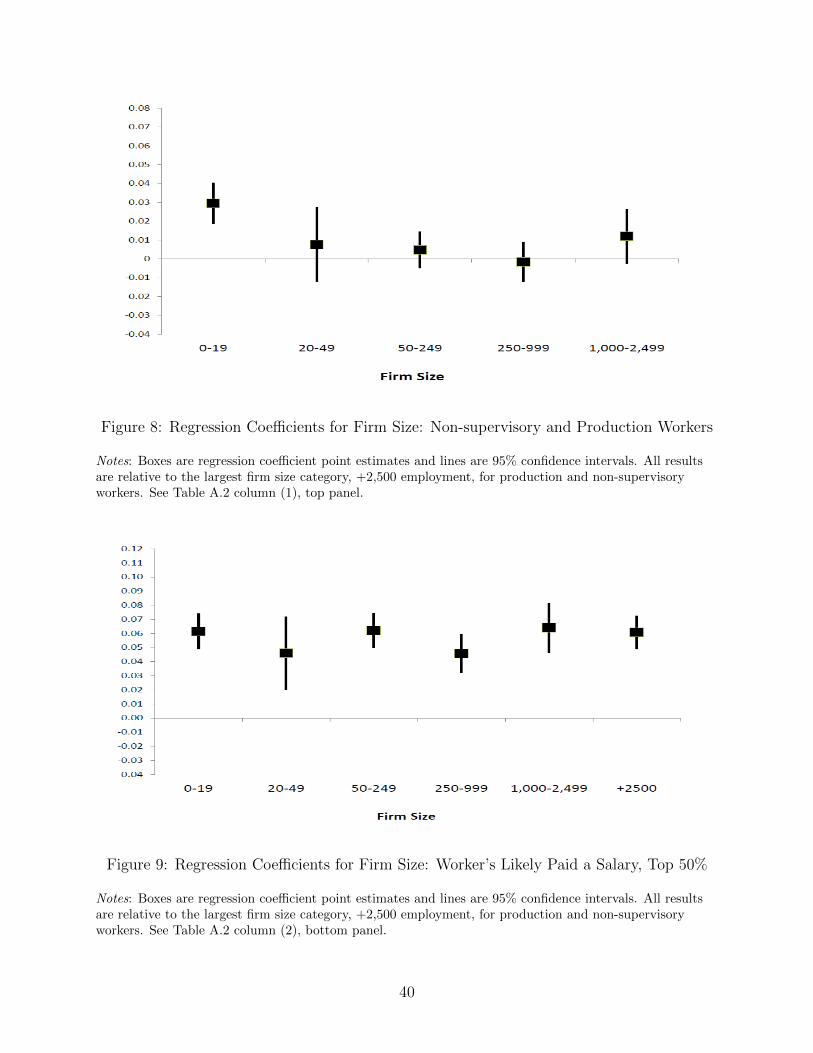
Figure 8: Regression Coefficients for Firm Size: Non-supervisory and Production Workers
Notes: Boxes are regression coefficient point estimates and lines are 95% confidence intervals. All resultsare relative to the largest firm size category, +2,500 employment, for production and non-supervisoryworkers. See Table A.2 column (1), top panel.
Figure 9: Regression Coefficients for Firm Size: Worker’s Likely Paid a Salary, Top 50%
Notes: Boxes are regression coefficient point estimates and lines are 95% confidence intervals. All resultsare relative to the largest firm size category, +2,500 employment, for production and non-supervisoryworkers. See Table A.2 column (2), bottom panel.
40
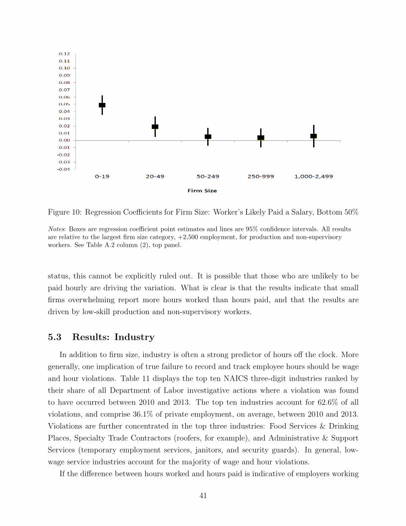
Figure 10: Regression Coefficients for Firm Size: Worker’s Likely Paid a Salary, Bottom 50%
Notes: Boxes are regression coefficient point estimates and lines are 95% confidence intervals. All resultsare relative to the largest firm size category, +2,500 employment, for production and non-supervisoryworkers. See Table A.2 column (2), top panel.
status, this cannot be explicitly ruled out. It is possible that those who are unlikely to be
paid hourly are driving the variation. What is clear is that the results indicate that small
firms overwhelming report more hours worked than hours paid, and that the results are
driven by low-skill production and non-supervisory workers.
5.3 Results: Industry
In addition to firm size, industry is often a strong predictor of hours off the clock. More
generally, one implication of true failure to record and track employee hours should be wage
and hour violations. Table 11 displays the top ten NAICS three-digit industries ranked by
their share of all Department of Labor investigative actions where a violation was found
to have occurred between 2010 and 2013. The top ten industries account for 62.6% of all
violations, and comprise 36.1% of private employment, on average, between 2010 and 2013.
Violations are further concentrated in the top three industries: Food Services & Drinking
Places, Specialty Trade Contractors (roofers, for example), and Administrative & Support
Services (temporary employment services, janitors, and security guards). In general, low-
wage service industries account for the majority of wage and hour violations.
If the difference between hours worked and hours paid is indicative of employers working
41
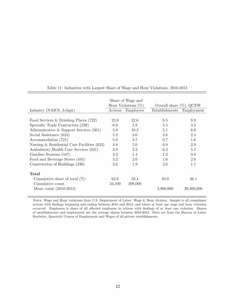
Table 11: Industries with Largest Share of Wage and Hour Violations, 2010-2013
Share of Wage andHour Violations (%) Overall share (%), QCEW
Industry (NAICS, 3-digit) Actions Employees Establishments Employment
Food Services & Drinking Places (722) 22.8 22.6 6.5 8.9Specialty Trade Contractors (238) 6.0 5.8 5.5 3.2Administrative & Support Services (561) 5.9 10.2 5.1 6.8Social Assistance (624) 5.2 3.6 3.6 2.4Accommodation (721) 5.0 3.7 0.7 1.6Nursing & Residential Care Facilities (623) 4.8 5.0 0.8 2.9Ambulatory Health Care Services (621) 3.9 3.2 6.3 5.7Gasoline Stations (447) 3.3 1.4 1.2 0.8Food and Beverage Stores (445) 3.2 2.0 1.6 2.6Construction of Buildings (236) 2.6 1.9 2.6 1.1
TotalCumulative share of total (%) 62.6 59.4 33.9 36.1Cumulative count 34,100 398,000Mean count (2010-2013) 2,980,000 39,400,000
Notes: Wage and Hour violations from U.S. Department of Labor, Wage & Hour division. Sample is all complianceactions with findings beginning and ending between 2010 and 2013, and where at least one wage and hour violationoccurred. Employees is share of all affected employees in actions with findings of at least one violation. Sharesof establishments and employment are the average shares between 2010-2013. Data are from the Bureau of LaborStatistics, Quarterly Census of Employment and Wages of all private establishments.
42

low-wage workers more than they report, this should be concentrated in the industries dis-
played in Table 11. To test this hypothesis, I create three indicator variables that evaluate
to unity if an ACS respondent’s LEHD dominant job is in one of the top ten, top five, or top
three NAICS 3-digit industries by share of enforcement actions, respectively. I fit equation
3 separately for each of the three indicator variables including demographic, job, firm, and
local labor market controls. The hypothesis is that the progression to industries with higher
concentrations of wage and hour violations should yield increased incidence of off the clock
work.
The results of this exercise are displayed in Table 12. The first column shows the results of
the indicator variable, denoted “High Incidence of Violation”, for the top ten industries. The
coefficient estimate is 0.0016 (0.0037), indicating workers report working 0.16% more hours
in these industries, although with little precision. Moving to column (2) and concentrating
on the top 5 industries, the estimate is now precise and 1.54% (0.0037) higher than in other
industries. Finally, column (3) focuses on the top 3 industries, which account for over a third
of enforcement actions. Again, the coefficient estimate is precise and increases, as expected,
with workers in these industries reporting working 3.04% (0.0035) more than they are paid.
Table 12: Off the Clock Work by Industry
(1) (2) (3)Top 10 Top 5 Top 3
High Incidence of Violation 0.0016 0.0154*** 0.0304***(0.0037) (0.0037) (0.0035)
R2 0.137 0.137 0.138
Notes: N = 218, 000. Dependent variable is the difference between logannual ACS hours calculated at 52 weeks and log annual LEHD hours.“High Incidence of Violation” is an indicator variable, which evaluates tounity if the LEHD dominant job is in the top 10, 5, or 3 NAICS 3-digitindustries ranked by incidence of wage and hour violations. See Table 11for ranking and details. All regressions estimated using OLS, and includefirm, job, demographic, and local labor market controls. Cluster-robuststandard errors clustered by state-firm. Stars on standard errors accordto p-values as follows: *** p<0.01, ** p<0.05, * p<0.1.
6 Conclusion
This study uses a unique dataset of person-level survey responses of hours worked linked
to the person’s employer reports of hours paid. To the best of my knowledge, this is the first
43

study in United States linking hours worked to administrative reports of hours paid at the
person-level. I interpret this as a measure of work off the clock. I use the measure to test
various theories of employer-employee bargaining.
I differentiate efficiency wage and labor hoarding theories of hours bargaining by test-
ing the association of off the clock work with cross-section variation in local labor market
slack. The hypothesis that greater work time off the clock may have a significant impact on
measured productivity is not supported by the empirical findings of this study. The results
find support for labor hoarding, though the effect is small. I find further evidence that the
cyclical component of work off the clock is driven by low-skill workers likely paid by the
hour.
The results also contribute to the emerging literature on labor compliance, and specifically
on more explicit determinants of work off the clock. In line with previous studies, I find
evidence that smaller firms are more likely to have employees report higher hours worked
compared to hours paid. The results indicate that for the smallest firms, work off the clock
is driven by production and non-supervisory employees.
At a broader level this study argues that hours of work should become a more prominent
topic in labor economic research. The measurement of hours is important for the study of
wages and productivity, and the often times casual tracking of hours by firms and workers
leads to failures of labor market compliance. Finally, this paper also advises caution when
using data on hours. The greater emphasis the economics profession is placing on adminis-
trative data combined with casual hours reporting by firms may produce misleading results
when using administrative data on hours. More stringently tracking hours worked for both
hourly and non-hourly workers would be an appropriate policy response. This will help both
administrative data collection and analysis, and may also have the beneficial effect of greater
wage and hour compliance.
References
Aaronson, S. and A. Figura (2010). How biased are measures of cyclical movements inproductivity and hours? Review of Income and Wealth 56 (3), 539–558.
Abowd, J. M., B. E. Stephens, L. Vilhuber, F. Andersson, K. L. McKinney, M. Roemer, andS. Woodcock (2009). The LEHD Infrastructure Files and the Creation of the QuarterlyWorkforce Indicators. In T. Dunne, J. B. Jensen, and M. J. Roberts (Eds.), ProducerDyanamics: New Evidence from Micro Data, pp. 149–230. University of Chicago Press.
Abowd, J. M. and M. H. Stinson (2013). Estimating Measurement Error in Annual Job
44
Earnings: A Comparison of Survey and Administrative Data. Review of Economics andStatistics (August), —-.
Abraham, K. G., J. Haltiwanger, K. Sandusky, and J. R. Spletzer (2013). Exploring Dif-ferences in Employment between Household and Establishment Data. Journal of LaborEconomics 31 (S1), S129–S172.
Ashenfelter, O. and R. S. Smith (1979). Compliance with the Minimum Wage Law. Journalof Political Economy 87 (2), 333–350.
Autor, D. H. and M. G. Duggan (2003). The rise in the disability rolls and the decline inunemployment. Quarterly Journal of Economics 118 (1), 157–206.
Bartik, T. J. (1991). Who Benefits from State and Local Economic Development Policies?W.E. Upjohn Institute for Employment Research.
Basu, A. K., N. H. Chau, and R. Kanbur (2010). Turning a Blind Eye: Costly Enforcement,Credible Commitment and Minimum Wage Laws. The Economic Journal 120 (543), 244–269.
Baum-Snow, N. and D. Neal (2009). Mismeasurement of usual hours worked in the censusand ACS. Economics Letters 102 (1), 39–41.
Bernhardt, A., M. Spiller, and N. Theodore (2013). Employers gone rogue: Explaining indus-try variation in violations of workplace laws. Industrial and Labor Relations Review 66 (4),808–832.
Biddle, J. E. (2014). Retrospectives: The Cyclical Behavior of Labor Productivity and theEmergence of the Labor Hoarding Concept. Journal of Economic Perspectives 28 (2),197–212.
Blanchard, O. J. and F. Katz (1991). Regional Revolutions. Brookings Papers on EconomicActivity (1), 1–75.
Bound, J., C. Brown, G. J. Duncan, and W. L. Rodgers (1994). Evidence on the Validity ofCross-Sectional and Longitudinal Labor Market Data. Journal of Labor Economics 12 (3),345.
Bound, J., C. Brown, and N. Mathiowetz (2001). Measurement error in survey data. InJ. Heckman and E. Leamer (Eds.), Handbook of Econometrics, Volume 5, Chapter 59, pp.3705–3843. Elsevier Masson SAS.
Bound, J. and H. J. Holzer (2000). Demand Shifts, Population Adjustments, and LaborMarket Outcomes during the 1980s. Journal of Labor Economics 18 (1), 20–54.
Bound, J. and A. B. Krueger (1991). The Extent of Measurement Error in LongitudinalEarnings Data: Do Two Wrongs Make a Right? Journal of Labor Economics 9 (1), 1.
Burda, M., K. R. Genadek, and D. S. Hammermesh (2016). Not Working at Work. NBERWorking Paper Series 21923.
45
Caballero, B. R. J., E. M. R. A. Engel, and J. Haltiwanger (1997). American EconomicAssociation Aggregate Employment Dynamics : Building from Microeconomic Evidence.The American Economic Review 87 (1), 115–137.
Caballero, R. J. and E. M. R. A. Engel (1993). Microeconomic Adjustment Hazards andAggregate Dynamics. The Quarterly Journal of Economics 108 (2), 359–383.
Cameron, A. C. and D. L. Miller (2015). A Practitioner’s Guide to Cluster- Robust Inference.Journal of Human Resouces 50 (2), 317–372.
Chang, Y.-m. and I. Ehrlich (1985). On the Economics of Compliance with the MinimumWage Law. Journal of Political Economy 93 (1), 84–91.
Cooper, R., J. Haltiwanger, and J. L. Willis (2007). Search frictions: Matching aggregateand establishment observations. Journal of Monetary Economics 54 (SUPPL.), 56–78.
Duncan, G. J. and D. H. Hill (1985). An Investigation of the Extent and Consequences ofMeasurement Error in Labor-Economic Survey Data. Journal of Labor Economics 3 (4),508.
Eldridge, L. P. and S. W. Pabilonia (2010). Bringing work home: implications for {BLS}productivity measures, Monthly Labor Review Online, December 2010. Monthly LaborReview 133 (12), 18–35.
Fair, R. C. (1969). The Short-Run Demand for Workers and Hours. Amsterdam: North-Holland Publishing Company.
Frazis, H. and J. Stewart (2004). What can time-use data tell us about hours of work.Monthly Labor Review. (December), 3–9.
Frazis, H. and J. Stewart (2009). Comparing Hours per Job in the CPS and the ATUS.Social Indicators Research 93 (1), 191–195.
Frazis, H. and J. Stewart (2010). Why Do BLS Hours Series Tell Different Stories aboutTrends in Hours Worked? In K. G. Abraham, J. R. Spletzer, and M. Harper (Eds.), Laborin the New Economy, Number October, pp. 343–372. University of Chicago Press.
Haltiwanger, J. C., S. J. Davis, and S. Shuh (1996). Job Creation and Job Destruction.Cambridge, MA: MIT Press.
Hamermesh, D. S. (1989). Labor Demand and the Structure of Adjustment Costs. TheAmerican Economic Review 79 (4), 674–689.
Ji, M. and D. Weil (2015). The Impact of Franchising on Labor Standards Compliance. ILRReview 68 (5), 977–1006.
Kalecki, M. (1943). Political Aspects of Full Employment. Political Quarterly 14, 322–330.
Lazear, E. P., K. L. Shaw, and C. Stanton (2015). Making Do with Less: Working Harderduring Recessions. Journal of Labor Economics 34 (1), 1–44.
46
Mellow, W. and H. Sider (1983). Accuracy of Response in Labor Market Surveys: Evidenceand Implications. Journal of Labor Economics 1 (4), 331.
Mendeloff, J., C. Nelson, K. Ko, and A. Haviland (2006). Small Businesses and WorkplaceFatality Risk: An exploratory analysis. Technical report, Rand Corporation.
Meyer, B. D. and R. M. Goerge (2011). Errors in Survey Reporting and Imputation andtheir Effects on Estimates of Food Stamp Program Participation.
Milkman, R., A. L. Gonzalez, and P. Ikeler (2012). Wage and hour violations in urbanlabour markets: a comparison of Los Angeles, New York and Chicago. Industrial RelationsJournal 43 (5), 378–398.
Oi, W. Y. (1962). Labor as a Quasi-Fiexed Factor. Journal of Political Economy 70 (6),538–555.
Rebitzer, J. B. (1987). Unemployment, Long-Term Employment Relations, and ProductivityGrowth. The Review of Economics and Statistics 69 (4), 627–635.
Rubin, D. B. (1987). Multiple Imputation for Nonresponse in Surveys. New York: JohnWiley & Sons.
Schaller, J. S. (2016). Booms , Busts , and Fertility: Testing the Becker Model Using Gender-Specific Labor Demand. The Journal of Human Resources 51 (1), 1–29.
Shapiro, C. and J. E. Stiglitz (1984). Equilibrium Unemployment as a Worker DesciplineDevice. American Economic Review 74 (3), 433–444.
Tibshirani, R. (1996). Regression Selection and Shrinkage via the Lasso. Journal of theRoyal Statistical Society B 58 (1), 267–288.
Tornqvist, L., P. Vartia, and Y. O. Vartia (1985). How Should Relative Changes Be Mea-sured? The American Statistician 39 (1), 43–46.
U.S. Bureau of Labor Statistics (2004). Construction of Average Weekly Hours for Super-visory and Nonproduction Wage and Salary Workers in Private Nonfarm Establishments.Technical report, Bureau of Labor Statistics.
Wagner, D. and M. Layne (2014). The Person Identificatoin Validation System (PVS):Applying the Center for Administrative Records Research and Applications’ (CARRA)Record Linkage Software.
Weil, D. (1991). Enforcing OSHA: The Role of Labor Unions. Industrial Relations 30 (1),20–36.
Weil, D. (2010). Improving Workplace Conditions Through Strategic Enforcement: A Reportto the Wage and Hour Division. Technical report.
47

Appendices
A Models of Efficiency Wages and Labor Hoarding
A.1 Model of Increased Worker Effort
The model is intentionally simple, and as such does not present a formal theory of unem-
ployment determination, or any equilibrium outcomes. What it does is clarify the continuous
implicit bargain between workers and firms, and give intuition for the difference between
hours worked and hours paid. The model is similar to the one presented in Lazear et al.
(2015), but here effort takes the form of hours worked above what is explicitly recorded by
employers. Workers are assumed to be paid a fixed salary implying that their wage is really
a gross earnings measure quoted over a fixed period that does not vary with hours worked.
Employer-recorded weekly hours are therefore an estimate usually determined by prevailing
laws and/or employer knowledge. In the United States, it is typical for a salaried employee to
be quoted a salary on a yearly basis (usually paid every two weeks or twice per month), with
40 hours per week that is loosely monitored by the employer. Workers therefore have some
latitude to choose the hours they actually work in a given week, trading off their distaste for
work against employers’ expectations of output.
In the model, time is discrete and workers are already matched with firms for a negotiated
period earnings measure, which I assume is fixed. Workers are exempt from overtime and
employers assume workers put in at least the statutory overtime limit of h hours. Employers
would like to terminate employees deemed to be shirking. Employers monitor worker effort
and they use observed hours as a proxy, whether perfectly observed, or a noisy measure.
For example, a worker who chooses not to show up to work stands a high risk of being
fired. Conversely, a worker who chooses to put in more hours likely produces more, and
sends a (possibly) valuable signal to employers about her ability to produce, which reduces
her probability of being fired. I define the function P (h) : R+ → [0, 1] ⊂ R, which maps
hours worked to the probability a worker retains her job in a given period. The probability
of retention is an increasing and concave function of hours worked with P (0) = 0 and
P ′(h) > 0, P ′′(h) < 0.
Putting forth effort is costly for workers, both because work is generally unpleasant, and
because workers are paid a lump sum regardless of how many hours they actually work.
Therefore, workers would prefer to work as little hours as possible. I capture the cost to
workers of putting forth greater effort by the function c(h) : R+ → R+. The costs to greater
working hours are increasing and convex with c(0) = 0 and c′(h) > 0, c′′(h) > 0. In addition
48
to the direct costs of more hours, workers must also weigh the costs of unemployment. More
specifically, the costs of losing one’s job in times of greater labor market slack are much
greater than when labor markets are tight, and the probability of contacting and finding a
suitable job is much higher. Define the unemployment rate by u, which both employers and
workers take as given. Further, define the option value of search from unemployment by R.
Although this sounds like the beginnings of a rudimentary search model, no formal theory
of of the aggregate determination of vacancies, unemployment and search will be presented
here.
Workers choose the optimal hours to work conditional on the explicit costs of working
and the indirect costs of aggregate labor market conditions. The problem of the worker is
maxh
V (h) = P (h) [W − c(h)] + (1− P (h))(1− u)R , (A.1)
where W is the gross earnings in the period, and V (h) is the asset value to the worker of
holding the job. The worker chooses the optimal hours of work to maximize A.1. Using the
first order condition and the implicit function theorem yields the following equation,
∂h
∂u= −P
′(h)R∂2V (h)
∂h
> 0 . (A.2)
The inequality follows from the fact that W − c(h) > (1− u)R in order for the employment
relationship to continue. Higher unemployment leads to greater hours worked.
Intuitively, hours increase in order to the decrease the probability of being fired, due to
the decrease in the payoff from unemployment. The second term in equation A.1 gives the
value of outside employment, R. As the probability of ascending to employment decreases –
as u increases – workers put forth more hours to avoid unemployment. With the employer’s
report of hours paid fixed at h, higher unemployment rates lead to a greater spread between
hours worked and hours paid.
A.2 Model of Labor Hoarding
The labor hoarding model is best conceptualized using a model of labor demand with
adjustment costs to employment. I describe the problem and the result loosely through the
“gap approach” (Caballero and Engel, 1993; Caballero et al., 1997). Consider a firm whose
production technology in a period uses only total labor inputs f (mt), with fm (·) > 0, and
mt = etht, where et is total employment and ht is average hours worked. I assume there is
an upper bound on the average hours worked per worker in a period so that firms seek to
employ more than one worker. Further, define h as the long-run average hours per employee
49
in the firm. For the purposes of this discussion, we can assume h = 40 and that these
are recorded by the firm as hours paid regardless of actual hours worked. Production faces
aggregate shocks At drawn from a probability distribution F (A). I assume only that the
probability distribution and production function are such that fA (·) > 0, which implies that
negative aggregate shocks should lead to decreased production in the absence of adjustment
costs.
Consider a firm faced with negative aggregate demand shock in the next period. Suppose
the current period’s employment as et−1 and without a loss of generality that ht−1 = h.
Following the gap approach, define e∗t as the frictionless optimal employment target for next
period given the realization of the negative aggregate demand shock. This is the optimal
employment for the firm if for the current period, and the current period only, the firm
did not have to pay any costs to adjust employment. Given the nature of the production
function, it holds that e∗t ≤ et−1, and et ∈ [e∗t , et−1]. In other words, the optimal employment
level given the shock will be bounded above by the current employment level, and bounded
below by the optimal frictionless level. The firm would like to get as close to its optimal
production level as possible, but in most cases the optimal employment level will lie above
the frictionless level. Thus, firms will adjust average hours down in order to further decrease
production beyond what was possible by only adjusting labor yielding ht ≤ ht−1. The same
logic, but in the opposite direction holds for a positive aggregate demand shock.
Putting this altogether, we see that a negative aggregate demand shock leads to less
hours worked. Note that in this model employment and hours move in the same direction in
response to a negative aggregate demand shock. The empirical results posit a relationship
between labor market slack and the difference between hours paid and hours worked. Given
the model, we need to assume the unemployment rate is negatively correlated with aggregate
demand shocks. That is, a positive demand shock produces non-positive movement in the
unemployment rate. This assumption seems straightforward.
To wrap up, a negative aggregate demand shock raises unemployment and forces firms
to cut production as well as raising the unemployment rate. Employment cannot fall to its
frictionless level so firms reduce hours worked to get closer to the optimal level of output.
As long as hours paid stay near constant, this produces the desired empirical test of greater
labor market slack and a non-positive gap between hours worked and hours paid.
B Details on Inverse Probability Weighting
The ACS links to the LEHD via a protected identification key (PIK). A PIK is a random
number mapped to a social security number, which serves as an internal Census Bureau
50
person-level identifier. PIK assignment is usually assumed to be correct, however survey
responses who fail to receive a PIK are known to be missing at random in the sense of Rubin
(1987).
Following (Meyer and Goerge, 2011) who point out that PIKs appear to be missing at
random, I use inverse probability weights to correct the ACS weights for PIKs missing at
random. I fit a probit model with a rich set of characteristics to predict the probability of
receiving a PIK. Using the fit model, I estimate the predicted probability for each cell, and
then multiply the ACS weights by the inverse of the probability of receiving a PIK for each
cell. Results obtained using weights adjusted in this manner differ very little from when they
are omitted. At no point do the qualitative findings change.
The terms of my data use for this project preclude the disclosure of ACS estimates
without commingled LEHD data. As such, I am not able to disclose the probit estimates
for the inverse probability weighting. The variables are summarized in Table A.4. However,
I am able to describe the key parameters qualitatively. In general, the included covariates
and results adhere closely to those used in Meyer and Goerge (2011).
The probability of receiving a PIK increases with age, likely due to greater work expe-
rience. The same holds true with education. The probability of receiving a PIK increases
with the highest level of educational attainment. People of color and Hispanics are slightly
less likely to receive a PIK than white non-Hispanics. Women and American citizens are
more likely to receive a PIK, while respondents who report speaking English “Well” or “Very
Well” are more likely to receive a PIK than respondents who report speaking English “Not
Well” or “Not at All”. Finally, respondents who did not move residences in the last year
have a higher probability of receiving a PIK than those who did.
C Details on Hourly/Nonhourly Imputation
Neither the ACS nor the LEHD datasets provide information on frequency or method
of pay for their earnings variables. This section describes the imputation of the probability
that an ACS respondent was not paid by the hour. This can include earnings or salaries paid
at annual, monthly, weekly or biweekly rate. This would also include workers who are paid
a piece rate. I use the Current Population Survey Outgoing Rotation Group (CPS ORG)
files, which asks respondents if they were paid by the hour or by some other arrangement on
their main job last week. I model the probability that a job is not paid by the hour using a
logit model, with covariates describing firm and job characteristics common to both the CPS
ORG and ACS. After fitting the model, I generate a predicted probability for each cell of
covariates. The final estimates are then attached to the ACS using the common covariates.
51

A more detailed explanation is offered below.
The CPS is a monthly survey of 60,000 households, which ask about labor market ac-
tivities during the previous week. Respondents are surveyed for four consecutive months,
they are then not interviewed for 8 months, and then they are reinterviewed for another
four months. The interviews conducted on the 4th and 8th months contain additional ques-
tions on earnings and hours for jobs worked the previous week. I use data from all months
from 2010-2013, which corresponds to the ACS years in my sample. I include only records
who worked in the private sector, state government, or local government. This discards
federal government workers, and the self-employed, neither of whom are included in the
ACS-LEHD matched sample. Finally, I keep only records for which the dependent variable,
“Hourly/Non-hourly status” is neither edited nor allocated.
To impute hourly/non-hourly pay, I fit a fully interacted least squares model with a
LASSO penalty. The LASSO provides a parsimonious model for both covariate shrinkage
and subset selection for an OLS model (Tibshirani, 1996). I use the LASSO in this setting
primarily as a tool for subset selection, using both five fold cross validation and the Akaike
information criterion (AIC) for selecting the LASSO parameter, which effectively chooses
the non-zero covariates in the model. Both methods return similar results, with the best
model including an indicator for whether a respondent has a Bachelor’s degree or more, and
an indicator for whether weekly earnings on the main job is in the top tercile of earnings, as
well as their interaction.
For the final imputation model I run a logit model interacting occupation, industry,
and tercile of weekly earnings. Although the LASSO indicated that a variable for Bachelor’s
degree or higher should be included, I omit it from the final imputation model for two reasons.
First, although highly correlated with non-hourly pay, there is no a priori reason for its
inclusion. Unlike weekly earnings, education is not part of the duties test for exemption from
overtime. Second, although correlated, I would like to evaluate education separately in the
statistical analysis. Including it in the non-hourly imputation would make the results hard
to identify and interpret. Finally, I include NAICS industry sectors and major occupation
groups in the final model. Job duties is one of the major tests for exemption from overtime,
which correlates highly with non-hourly status. Various industries carve out exemptions for
overtime and determine pay norms, which argues for its inclusion.
After fitting the model on the CPS, I attach the predicted probabilities for each cell to the
final analysis sample. Attaching major occupation groups and industry is straight forward.
I do not observe weekly earning for either the ACS or the LEHD. I calculate annual earnings
terciles based on the LEHD, and use that as the tercile to which I map weekly earnings.
This assumes the same weekly earnings is earned each week, which scales weekly earnings
52

to an annual earnings measure.53 I then bin each observation in the final analysis sample by
quartile of their likelihood of non-hourly pay.
Summary statistics for the analysis sample by quartile of non-hourly pay are available in
Table A.3. Based on prior knowledge and casual observation, the results are largely what
one would expect. Observations in the highest quartile of probability they are not paid
by the hour have much higher reported hours worked compared to hours paid averaging
14.3% assuming 52 weeks worked. In contrast, quartiles one through three are relatively
uniform with hours worked exceeding hours paid by 6.8%, 4.0%, and 6.3% for quartiles
one through three, respectively. The remaining stratifying variables change by quartile as
expected. Workers in the top quartile are much more likely to be white, male, and have a
Bachelor’s degree.
D Additional Tables and Figures
53Recall the final analysis sample is only for full-year workers.
53
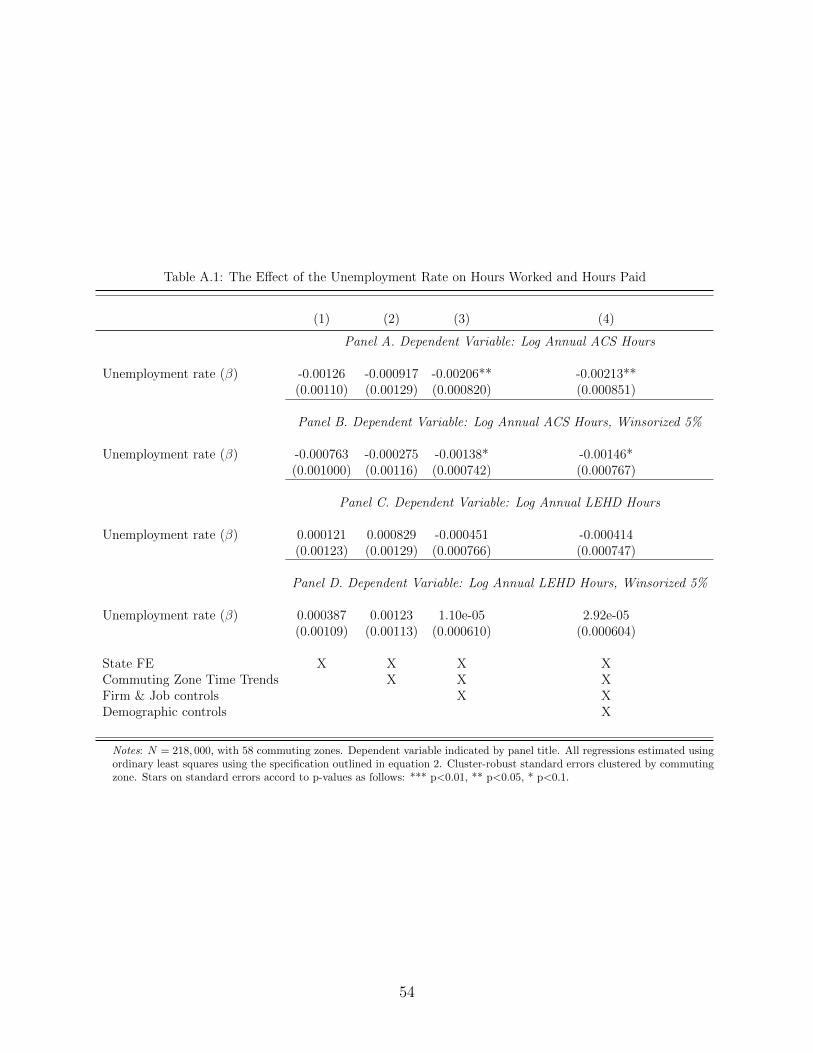
Table A.1: The Effect of the Unemployment Rate on Hours Worked and Hours Paid
(1) (2) (3) (4)
Panel A. Dependent Variable: Log Annual ACS Hours
Unemployment rate (β) -0.00126 -0.000917 -0.00206** -0.00213**(0.00110) (0.00129) (0.000820) (0.000851)
Panel B. Dependent Variable: Log Annual ACS Hours, Winsorized 5%
Unemployment rate (β) -0.000763 -0.000275 -0.00138* -0.00146*(0.001000) (0.00116) (0.000742) (0.000767)
Panel C. Dependent Variable: Log Annual LEHD Hours
Unemployment rate (β) 0.000121 0.000829 -0.000451 -0.000414(0.00123) (0.00129) (0.000766) (0.000747)
Panel D. Dependent Variable: Log Annual LEHD Hours, Winsorized 5%
Unemployment rate (β) 0.000387 0.00123 1.10e-05 2.92e-05(0.00109) (0.00113) (0.000610) (0.000604)
State FE X X X XCommuting Zone Time Trends X X XFirm & Job controls X XDemographic controls X
Notes: N = 218, 000, with 58 commuting zones. Dependent variable indicated by panel title. All regressions estimated usingordinary least squares using the specification outlined in equation 2. Cluster-robust standard errors clustered by commutingzone. Stars on standard errors accord to p-values as follows: *** p<0.01, ** p<0.05, * p<0.1.
54
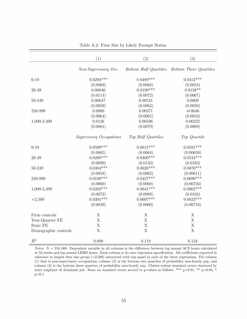
Table A.2: Firm Size by Likely Exempt Status
(1) (2) (3)
Non-Supervisory Occ. Bottom Half Quartiles Bottom Three Quartiles
0-19 0.0294*** 0.0489*** 0.0412***(0.0069) (0.0068) (0.0054)
20-49 0.00846 0.0190*** 0.0138**(0.0114) (0.0072) (0.0067)
50-249 0.00647 0.00521 0.0009(0.0059) (0.0062) (0.0050)
250-999 0.0000 0.00371 -0.0046(0.0064) (0.0065) (0.0053)
1,000-2,499 0.0126 0.00596 0.00232(0.0081) (0.0079) (0.0069)
Supervisory Occupations Top Half Quartiles Top Quartile
0-19 0.0599*** 0.0615*** 0.0591***(0.0065) (0.0064) (0.00659)
20-49 0.0280*** 0.0460*** 0.0534***(0.0099) (0.0133) (0.0163)
50-249 0.0384*** 0.0620*** 0.0870***(0.0058) (0.0062) (0.00611)
250-999 0.0198*** 0.0457*** 0.0690***(0.0060) (0.0068) (0.00756)
1,000-2,499 0.0202*** 0.0641*** 0.0902***(0.0073) (0.0089) (0.0103)
+2,500 0.0391*** 0.0607*** 0.0823***(0.0049) (0.0060) (0.00710)
Firm controls X X XYear-Quarter FE X X XState FE X X XDemographic controls X X X
R2 0.098 0.119 0.124
Notes: N = 218, 000. Dependent variable in all columns is the difference between log annual ACS hours calculatedat 52 weeks and log annual LEHD hours. Each column is its own regression specification. All coefficients reported inreference to largest firm size group (+2,500) interacted with top panel in each of the three regressions. For column(1) that is non-supervisory occupations, column (2) is the bottom two quartiles of probability non-hourly pay, andcolumn (3) is the bottom three quarters of probability non-hourly pay. Cluster-robust standard errors clustered bystate employer of dominant job. Stars on standard errors accord to p-values as follows: *** p<0.01, ** p<0.05, *p<0.1
55

Figure A.1: Distribution of the Difference of Log Labor Earnings (ACS) and Log LaborEarnings (LEHD) by Usual Weekly Hours
Notes: Variable is the difference in log ACS earnings from log LEHD earnings for the full sample,winsorized at the 5% and 95% level. The variable is partitioned by whether an ACS respondent answersthat she usually works either 1) less than 40 hours per work (top panel) or 2) exactly 40 hours a week(middle panel) or 3) more than 40 hours per week (bottom panel). Top panel N = 49, 000, middle panelN = 108, 000, bottom panel N = 61, 000. Mean of bottom panel −0.094 [0.318], middle panel −0.077[0.247] and bottom panel −0.078 [0.248].
56
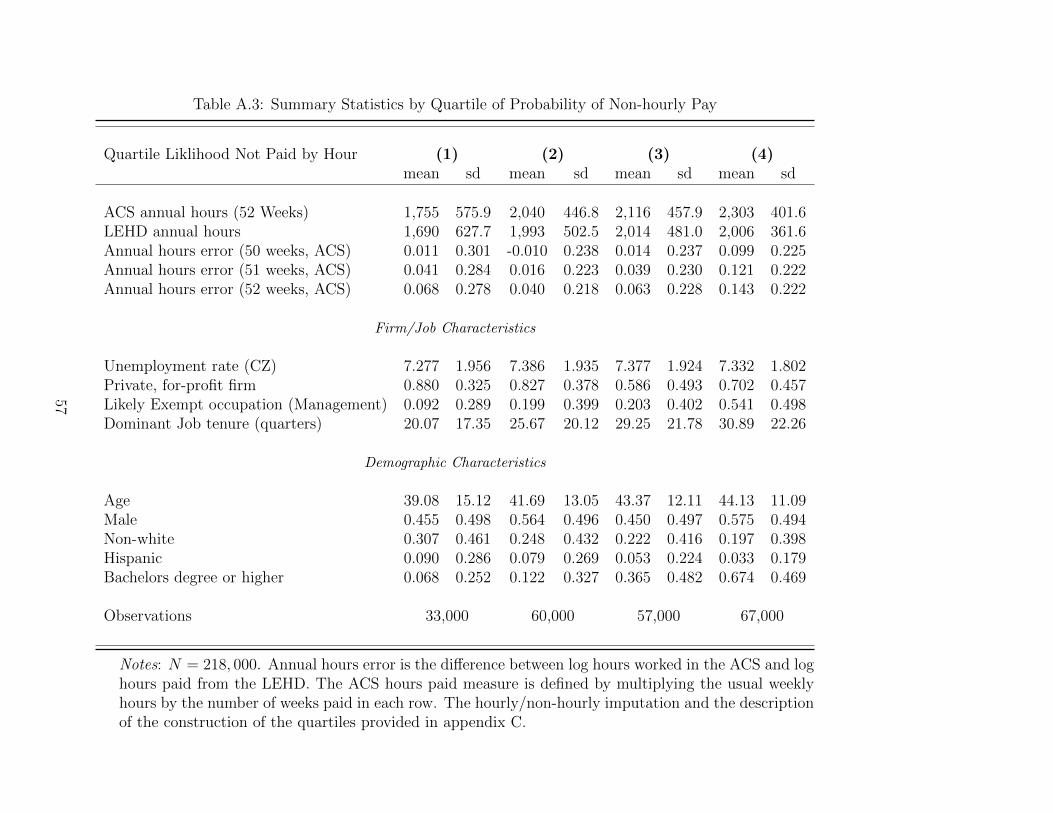
Table A.3: Summary Statistics by Quartile of Probability of Non-hourly Pay
Quartile Liklihood Not Paid by Hour (1) (2) (3) (4)mean sd mean sd mean sd mean sd
ACS annual hours (52 Weeks) 1,755 575.9 2,040 446.8 2,116 457.9 2,303 401.6LEHD annual hours 1,690 627.7 1,993 502.5 2,014 481.0 2,006 361.6Annual hours error (50 weeks, ACS) 0.011 0.301 -0.010 0.238 0.014 0.237 0.099 0.225Annual hours error (51 weeks, ACS) 0.041 0.284 0.016 0.223 0.039 0.230 0.121 0.222Annual hours error (52 weeks, ACS) 0.068 0.278 0.040 0.218 0.063 0.228 0.143 0.222
Firm/Job Characteristics
Unemployment rate (CZ) 7.277 1.956 7.386 1.935 7.377 1.924 7.332 1.802Private, for-profit firm 0.880 0.325 0.827 0.378 0.586 0.493 0.702 0.457Likely Exempt occupation (Management) 0.092 0.289 0.199 0.399 0.203 0.402 0.541 0.498Dominant Job tenure (quarters) 20.07 17.35 25.67 20.12 29.25 21.78 30.89 22.26
Demographic Characteristics
Age 39.08 15.12 41.69 13.05 43.37 12.11 44.13 11.09Male 0.455 0.498 0.564 0.496 0.450 0.497 0.575 0.494Non-white 0.307 0.461 0.248 0.432 0.222 0.416 0.197 0.398Hispanic 0.090 0.286 0.079 0.269 0.053 0.224 0.033 0.179Bachelors degree or higher 0.068 0.252 0.122 0.327 0.365 0.482 0.674 0.469
Observations 33,000 60,000 57,000 67,000
Notes: N = 218, 000. Annual hours error is the difference between log hours worked in the ACS and loghours paid from the LEHD. The ACS hours paid measure is defined by multiplying the usual weeklyhours by the number of weeks paid in each row. The hourly/non-hourly imputation and the descriptionof the construction of the quartiles provided in appendix C.
57

Table A.4: Covariates in Inverse Probability Weighting Probit
Variable Description
Gender Indicator for whether male.Age 16-19, 20-34, 35-49, 50-65, 65+Education Less than high school, High School, Some College, BA+White Indicator for whether race is whiteHispanic Indicator for hispanic ethnicityCitizen Indicator for whether U.S. citizenMarried Indicator for whether marriedKids Indicator for presence of own childrenMoved Indicator for whether moved in last yearDisability Indicator for whether has a disabilityEnglish Indicator for whether speaks English ”Very well” or ”Well”Labor Force Indicator for whether in labor force
Notes: Variables used for reweighting sample weights to account for PIKs missing at random. All variablesare indicator variables unless otherwise noted. Construction and use of the weights is described inappendix B.
58
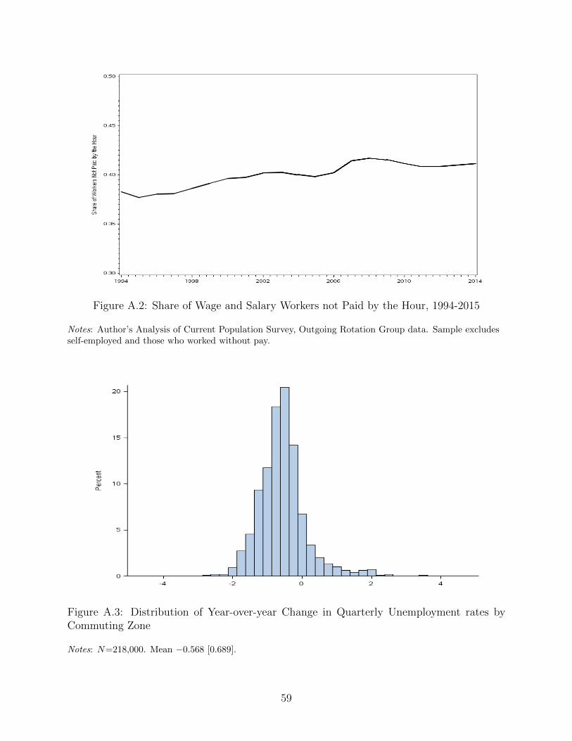
Figure A.2: Share of Wage and Salary Workers not Paid by the Hour, 1994-2015
Notes: Author’s Analysis of Current Population Survey, Outgoing Rotation Group data. Sample excludesself-employed and those who worked without pay.
Figure A.3: Distribution of Year-over-year Change in Quarterly Unemployment rates byCommuting Zone
Notes: N=218,000. Mean −0.568 [0.689].
59

Table A.5: Regression Results for Unemployment Rate and Work Off the Clock, Heterogeneous Effects Subsets
(1) (2) (3) (4) (5) (6)Top half Bottom half At least Less than
likely paid likely paid B.A. B.A.Supervisory Non-Supervisory non-hourly non-hourly degree degree
Unemployment rate (β) -0.00097 -0.00213* -0.00107 -0.00287* 0.00000 -0.00231**(0.00138) (0.00112) (0.00120) (0.00151) (0.00126) (0.00099)
Observations 74,000 145,000 131,000 87,000 75,000 143,000R2 0.133 0.070 0.129 0.096 0.125 0.075
Notes: N = 218, 000, with 58 commuting zones. Dependent variable is the difference between log annual ACS hours calculated at52 weeks and log annual LEHD hours. Supervisory, Column (1), refers to the compliment of non-supervisory. The definition ofnon-supervisory or production worker comes from the Bureau of Labor Statistics. Column (2), Non-supervisory, is an indicatorfor observations who meet the definition of a production or non-supervisory worker according to the occupation and industryof her dominant job. “Bottom half likely paid non-hourly”, Column (3), refers to observations who are below the median inlikelihood they are not paid by the hour. “Top half likely paid non-hourly”, Column (4), refers to observations above the medianlikelihood not paid by the hour. B.A refers to Bachelor’s degree. All regressions run using OLS with the same specification asTable 2 column (4), subset to cell listed at the top of each column. Cluster-robust standard errors clustered by commuting zone.Stars on standard errors accord to p-values as follows: *** p<0.01, ** p<0.05, * p<0.1.
60
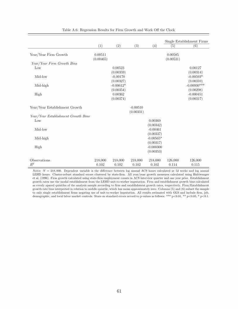
Table A.6: Regression Results for Firm Growth and Work Off the Clock
Single Establishment Firms(1) (2) (3) (4) (5) (6)
Year/Year Firm Growth 0.00511 0.00585(0.00465) (0.00531)
Year/Year Firm Growth BinsLow 0.00523 0.00127
(0.00359) (0.00314)Mid-low -0.00170 -0.00593*
(0.00327) (0.00310)Mid-high -0.00612* -0.00930***
(0.00354) (0.00298)High 0.00362 -0.000451
(0.00374) (0.00317)
Year/Year Establishment Growth -0.00510(0.00331)
Year/Year Establishment Growth BinsLow 0.00369
(0.00342)Mid-low -0.00461
(0.00337)Mid-high -0.00565*
(0.00317)High -0.000300
(0.00353)
Observations 218,000 218,000 218,000 218,000 126,000 126,000R2 0.102 0.102 0.102 0.102 0.114 0.115
Notes: N = 218, 000. Dependent variable is the difference between log annual ACS hours calculated at 52 weeks and log annualLEHD hours. Cluster-robust standard errors clustered by state-firm. All year/year growth measures calculated using Haltiwangeret al. (1996). Firm growth calculated using state-firm employment counts in ACS interview quarter and one year prior. Establishmentgrowth rates use the modal establishment from the LEHD unit-to-worker imputation. Firm and establishment growth bins calculatedas evenly spaced quintiles of the analysis sample according to firm and establishment growth rates, respectively. Firm/Establishmentgrowth rate bins interpreted in relation to middle quintile, which has mean approximately zero. Columns (5) and (6) subset the sampleto only single establishment firms negating use of unit-to-worker imputation. All results estimated with OLS and include firm, job,demographic, and local labor market controls. Stars on standard errors accord to p-values as follows: *** p<0.01, ** p<0.05, * p<0.1.
61
Top Related