


Languages
Pages
Legal


Higher education as a portfolio investment:students’ choices about studying, termtime employment, leisure, and loans
By Jim Pemberton*, Sarah Jewelly, Alessandra Faggianz, andZella King�
*School of Economics, University of Reading
ySchool of Economics, University of Reading, PO Box 218, Reading RG6 6AA;
e-mail: [email protected]
zAED Economics, The Ohio State University, Columbus, OH 43210, USA
�Henley Business School, University of Reading
Recent UK changes in the number of students entering higher education, and in the
nature of financial support, highlight the complexity of students’ choices about human
capital investments. Today’s students have to focus not on the relatively narrow issue
of how much academic effort to invest, but instead on the more complicated issue of
how to invest effort in pursuit of ‘employability skills’, and how to signal such acqui-
sitions in the context of a highly competitive graduate jobs market. We propose a
framework aimed specifically at students’ investment decisions, which encompasses
corner solutions for both borrowing and employment while studying.
JEL classifications: J22, J24, I23.
1. IntroductionThis paper analyses student choices in higher education (HE). It argues that
these are more complex than implied by existing literature, and develops a new
framework. We motivate the discussion by considering recent changes in the UK’s
HE system, which is reasonably representative of HE in the developed world in
most respects.1
Over the past two decades life for UK HE students has become much more
complex. Twenty years ago most were financially supported by a mixture of
non-repayable state grants and parental transfers, and whilst many supplemented
this with vacation earnings, term-time work was relatively unusual. Thus, for most
..........................................................................................................................................................................1 An exception is the nature and extent of student financial support, where there is sufficient diversity
among countries that no one country can reasonably be regarded as fully representative. The OECD
provides a good empirical survey of HE systems across the developed world (OECD 2009).
! Oxford University Press 2012All rights reserved
Oxford Economic Papers 65 (2013), 268–292 268doi:10.1093/oep/gps026
at Ohio State U
niversity Prior Health Sciences L
ibrary on June 21, 2013http://oep.oxfordjournals.org/
Dow
nloaded from

HE students their only important decision was the amount of effort to invest in
studying, and thereby in the quality of degree obtained, indicated by degree clas-
sification. A reasonable quality of degree in turn, provided near-automatic entry to
a graduate level job.
This simple world has largely disappeared because of two fundamental changes:
in sector size (a rise in the proportion of 18–20 year olds in HE from 6% in 1960
(Blanden and Machin, 2004) to 34% in 2006 (DIUS, 2009)); and in funding (the
replacement of most student grants by state-backed student loans repayable from
future earnings, as well as the introduction of tuition fees in 1998). Increased sector
size means that a degree is no longer a semi-automatic passport to a ‘graduate job’,
because the much increased number of graduates makes it difficult for employers to
identify the strongest candidates (Brown and Hesketh, 2004). Consequently, many
students seek to acquire additional forms of human capital, e.g., work experience,
to try to distinguish themselves from other candidates The UK Confederation of
British Industry provides a substantial survey of employer and student attitudes
which indicates that both groups now pay at least as much, perhaps more, attention
to ‘employability skills’ (e.g., self-management, team working, business awareness,
and problem-solving) as to the quality of degree result (CBI, 2009; see also Purcell
et al., 2002; Dickerson and Green, 2004). Hence today’s students face a more
complex investment decision than their predecessors: they have to invest time
and effort in a portfolio of activities, not just academic study; and they also need
to consider how best to signal such acquisitions in a highly competitive graduate
jobs market.
The switch from grants to repayable loans has also complicated students’
lives. Today’s students have to make more complex financial decisions than their
predecessors, involving choices between loans and term-time working as alternative
sources of income. Loans impose future repayment costs; term-time work may
reduce degree quality if it eats too much into study time (Jones and Sloane,
2005; Purcell et al., 2005; Van Dyke et al, 2005). A TUC report found a 50%
increase between 1996 and 2006 in the number of UK students working during
term time (TUC, 2006). Overall, there is a much increased dependence of students
on income from paid employment and loans, particularly among lower social class
students (Callender and Kemp, 2000; Callender and Wilkinson, 2003; Van Dyke
et al., 2005; Finch et al., 2006). The average annual loan taken by students increased
from £1,530 in 1998 to £3,330 in 2006,2 with average student debt expected to rise
as a result of the Browne review3 and the introduction of higher variable fees of up
to £9,000.
Although the consequences of changes in sector size and in funding could be
viewed separately, our contention is that they are better viewed together, since they
are interconnected. This is well illustrated by term time employment, which
..........................................................................................................................................................................2 See http://www.slc.co.uk/statistics.aspx.3 See http://www.bis.gov.uk/assets/biscore/corporate/docs/s/10-1208-securing-sustainable-higher-educa
tion-browne-report.pdf.
pemberton et al. 269
at Ohio State U
niversity Prior Health Sciences L
ibrary on June 21, 2013http://oep.oxfordjournals.org/
Dow
nloaded from
(i) provides a potential alternative to student loans as a source of income for
(perhaps) debt-averse students; might also be a means both (ii) of gaining
additional forms of human capital, and (iii) of signalling specific skills to a
future graduate recruiter; but (iv) takes time away from studying and from
leisure. Our contention is that all these choices—size of loan, and allocations of
time to each of studying, employment, and leisure—should be analysed in a unified
framework, since each affects and is affected by all the others. The next section
reviews the literature on this issue, and outlines findings from a recent survey of
student choices which suggest particular patterns of choice that require explan-
ation. This motivates the development in Sections 3 and 4 of a unified framework
for analysing students’ investment decisions. Section 5 concludes.
2. Student choices in higher education: previous literatureThe massive human capital literature has largely ignored the sorts of student
investment choices, even when dealing specifically with UK graduates (e.g.,
Faggian and McCann, 2006), introduced in the previous section. We could find
only three relevant conceptual papers: Oettinger (2005), Kalenkoski and Pabilonia
(2010), and Neill (2006).4 Whilst each provides useful insights, they also ignore at
least one core element. Thus, Oettinger ignores student loans and other borrowing,
and also assumes that future employment prospects depend only on academic
qualifications; Kalenkoski and Pabilonia likewise ignore borrowing, and also
leisure; and Neill assumes that each student has to choose between either
additional studying (over and above a fixed minimum) or paid employment: in
her model students cannot choose combinations of some discretionary studying
and some paid employment (see Neill, 2006, p.13, footnote 19). Overall, therefore,
none of these studies adequately captures the interlocking nature of HE students’
decisions about borrowing, paid employment, studying, employability, and
leisure.5 Although the issues are conceptually similar to other human capital
choices, we believe that there is sufficient distinctiveness to justify a specific
framework.
This view is strengthened by the patterns of student choice revealed in a recent
survey of students in the UK. Jewell (2008) undertook a survey at a university based
in the southeast of England, which asked about family background, financial cir-
cumstances and student employment (predominately that undertaken during term
..........................................................................................................................................................................4 Although all three papers are conceptual rather than empirical, the Oettinger and Kalenkoski/Pabilonia
models are oriented towards the HE set-up in the USA, and the Neill model towards HE in Canada. The
recent UK trends outlined in Section 1 have moved the UK set-up nearer to those in USA and Canada.
Neill’s work builds on earlier work by Keane (2002) and Keane and Wolpin (2001); she uses an
augmented version of the Keane-Wolpin model.5 Although there is little such work set in the HE context, there is a large empirical literature on the
consequences of high school students’ (‘school’ students in UK terminology) part-time working for their
post-school earning capacity, e.g., Ruhm (1997), Light (2001), and Hotz et al. (2002). To date no
empirical consensus has emerged. Ruhm and Light both provide summaries.
270 higher education as portfolio investment
at Ohio State U
niversity Prior Health Sciences L
ibrary on June 21, 2013http://oep.oxfordjournals.org/
Dow
nloaded from

time). Survey data from 622 British domiciled students graduating in 2006 and
2007 were matched to their university personal record and information about their
labour market outcomes six months after graduation.6 A companion paper (Jewell
et al., 2010), which provides an econometric analysis of the consequences of
students’ employment choices on degree and labour market outcomes, analyses
patterns of student loan take-up and student term-time employment. For this
purpose the amount of term time employment was divided into five categories:
zero, low, medium, high, and very high intensity.7 Table 1 summarizes the dataset.
In interpreting Table 1 we note that both loans and term-time employment
normally have upper limits. In the UK, for example, the Student Loans
Company sets a maximum loan; this is Table 1’s ‘maximum loan’.8 As regards
employment, many UK HE institutions publish advisory limits on term-time
working. Even if some students consider disregarding such advice, practical
limits are still likely to result from studying constraints. We discuss this further
in the next section; for now we simply assume that a limit exists, that it is common
to all students, and that it is equal to the highest of the five term-time employment
levels (very high intensity).
Table 1 Student loans and term-time employment: patterns of choice
Intensity of term-timeemployment
Level of borrowing.....................................................................................
Total
No loan Less thanmaximum loan
Maximumloan
Zero 36 25 259 320Low intensity 5 6 60 71Medium intensity 3 5 59 67High intensity 5 3 58 66Very high intensity 16 8 74 98Total 65 47 510 622
Source: Jewell, 2008.
Notes: Each individual cell shows the number of students in the sample choosing the indicated com-
bination of employment intensity and borrowing level.
..........................................................................................................................................................................6 This information was obtained from their Destinations of Leavers in Higher Education (DLHE) survey
responses. The DLHE is undertaken by all universities to gather information on graduate destinations;
for more information see http://www.hesa.ac.uk/index.php/component/option,com_collns/task,
show_collns/targetYear,any/Itemid,231/targetStream,3/.7 These categories were based on hours and number of weeks worked, see Jewell (2008) for more
information.8 In principle students might be able to obtain additional borrowing from other sources, but any such
lenders are themselves likely to limit what they will lend. Our dataset has no information on non-SLC
borrowing. The idea of borrowing constraints is familiar from the literature on intertemporal household
saving; cf., Zeldes 1989, Deaton 1991.
pemberton et al. 271
at Ohio State U
niversity Prior Health Sciences L
ibrary on June 21, 2013http://oep.oxfordjournals.org/
Dow
nloaded from

With this interpretation Table 1 suggests that both term-time employment deci-
sions and student loans decisions are bi-modal, with most choices at the extremes
of the distributions. Looking first at student loans, the modal choice, made by 82%
of the sample, is to borrow the maximum amount. There is a second, albeit much
smaller, modal point at zero loans, chosen by 10% of students. Only 8% choose an
intermediate point. The same pattern applies to term-time working. The modal
choice, made by 51% of students, is zero working; again there is a second modal
point at the opposite extreme of the distribution, with 16% of students choosing
‘very high work intensity’. In between these two extremes, 11% of students are
located at each of three intermediate points. This suggests that the incentive
structure systematically pushes HE students towards corner solutions for both
loans and employment, with only a minority choosing interior solutions. Whilst
economic analysis readily accommodates corner solutions, it routinely focuses on
interior solutions and rarely develops models in which the modal choice for even
one, let alone two, variables is at a corner.9 From this perspective the seemingly
corner-dominated pattern of student choices merits further analysis.10
3. A model of students’ investment of time and effort3.1 The model
We use a two-period framework. The first period covers time at university
(typically three years in the UK); the second spans a similar length of time and
covers the early years of subsequent working life.11 We assume the following utility
..........................................................................................................................................................................9 As noted in the previous footnote, the literature on intertemporal household saving routinely incorp-
orates borrowing constraints, especially in the early stages of the life cycle, and this causes younger
individuals to locate at borrowing corners. This literature has never explored the possibility of
employment constraints, however, presumably because it typically focuses on individuals in full time
employment rather than on HE students.10The joint distribution of loan and work choices in the Jewell (2008) dataset is also worthy of note, since
the subset of students who choose the highest level of term time working (‘very high intensity’) includes
the lowest proportion of people students who choose the maximum loan (75%). This is hard to explain
if the only or primary motive for working is to fund current consumption (since then one would expect
those who need to work the most for this purpose to be the keenest to take out loans). It is of course
possible that the Jewell dataset, derived as it is from a single UK university, is unrepresentative of student
behaviour more widely within the UK or internationally. Data from the UK Student Loan Company
show that in 2005 79% of eligible UK students took out a loan, compared with 89% in the Jewell dataset,
suggesting that the latter is not substantially out of line, at least so far as the decision about whether or
not to take a loan is concerned. It is much harder to assess its representativeness as regards the amounts
and pattern of term-time working, because so far as we are aware there are no detailed national or
international data about this, so the only source of information is surveys at individual universities, and
even here information is usually limited because few such surveys include details of total hours worked
by individual students per week, month, and year. More detailed information about UK student loans is
available from the Student Loan Company: see http://www.slc.co.uk/statistics.aspx.11 We define the second period in this way because the Jewell (2008) dataset’s use of the DLHE data (cf.,
footnote 6) means that its measures of post-HE employment and wage outcomes focus only on
short-run outcomes rather than on lifetime earnings. Extending our model to cover lifetime earnings
272 higher education as portfolio investment
at Ohio State U
niversity Prior Health Sciences L
ibrary on June 21, 2013http://oep.oxfordjournals.org/
Dow
nloaded from
function for an individual student i:
UðiÞ ¼ log½C1ðiÞ� þ VðiÞ log½LðiÞ� þ DðiÞ log½C2ðiÞ� ð1Þ
C1(i) is consumption whilst at university, C2(i) is consumption in early working
life, L(i) is leisure time whilst at university, V(i) is the weight attached to leisure
relative to consumption, and D(i) is the rate of time discounting, with V(i)> 0 and
0<D(i)4 1. Leisure is a choice variable in period 1 but in period 2 we assume that
all students work for a fixed amount of time.12
We specify budget constraints as follows:
C1ði Þ ¼ WH1ði Þ þ Tði Þ þ Bði Þ
LðiÞ ¼ 1� H1ðiÞ � f ðiÞSðiÞ
C2ðiÞ ¼ W2ðiÞH2 � RBðiÞ
BðiÞ4Bmax; 04H1ðiÞ4Hmax < 1
ð2Þ
We assume a fixed total amount of time in period 1, normalized at unity, of
which a fraction H1(i) is spent in paid term-time employment at an exogenously
fixed wage W, and a fraction S(i)> 0 is spent studying. Hmax reflects our previously
mentioned assumption of an upper limit on the amount of term-time employment
which is the same for all students. We discuss this before considering the other
details of the budget constraints. The issues are well captured by the advice which
Imperial College currently gives its students:
The College recommends that full-time students do not take up part-time work duringterm-time. If this is unavoidable we advise students to work no more than 10–15hours per week, which should be principally at weekends and not within the normalworking hours of the College. Working in excess of these hours could impact adverselyon a student’s studies or health . . . The College does not condone situations where astudent’s employment would cause them to miss teaching or other departmentalactivity during the College working day, or submit coursework after the specifieddeadline . . . The College’s examination boards will not normally consider asmitigating circumstances any negative impact that part-time work during term-timemay have had on a student’s performance in examinations or in other assessed work.(Imperial College, Senate papers, November 2011).
If Imperial’s students follow its advice they will all have the same value for Hmax,
determined by Imperial’s 15-hour upper limit. Of course, some students might
consider ignoring it, even though the risks (both to degree quality and to health)
are clearly spelled out. In practice many, and probably most students, will struggle
..........................................................................................................................................................................would not in itself require any substantial re-specification. However, many of today’s students will
eventually themselves have children who enter HE, and will thus need to make their own decisions
about the size of parental transfer. Extending our model to longer periods would thus logically require
us to model such decisions using an overlapping generations framework. This would evidently
complicate the analysis and shift it away from our intended focus on intra-HE decision making.12 Excluding leisure from period 2 is partly for simplicity but also reflects data considerations: there is no
information about students’ post-HE leisure choices in the DLHE dataset (cf., footnotes 6 and 11) nor so
far as we are aware in any other available dataset.
pemberton et al. 273
at Ohio State U
niversity Prior Health Sciences L
ibrary on June 21, 2013http://oep.oxfordjournals.org/
Dow
nloaded from

to exceed the 15-hour limit by a significant amount even if they wish to do so,
because the lumpy and inflexible nature of academic programmes and part-time
jobs severely constrains daytime employability. Most academic programmes have
commitments scattered throughout the working week, leaving few if any sizeable
chunks of free time during the working day. This will make it difficult if not
impossible to find weekday daytime jobs whose requirements match student avail-
ability and which are also financially worthwhile if there are significant fixed costs
of travel between campus and workplace. Weekday evening or night-time jobs do
not pose the same problems, but are still subject to the health and academic per-
formance risks emphasized by Imperial College. Peak load academic commitments
(coursework deadlines, exam revision) exacerbate the difficulties: if students cannot
commit to working every week for a significant length of time their employability is
further reduced.
Overall, it seems plausible that few if any full-time students can work over a
sustained period for the equivalent of more than weekend daytime hours plus
occasional weekday evening hours, suggesting an effective limit not much above
Imperial’s 15-hour guidance. Some students in some circumstances might find
ways to work significantly longer hours, but normally only for limited periods of
time (e.g., during a non-exam term, or during one year of a three-year degree
programme). Bearing in mind that in our framework Hmax is appropriately inter-
preted as a maximum limit which is averaged over an entire degree programme
rather than as a limit which applies to each individual week or term, assuming a
common limit does not seem an unreasonable generalization.
Returning to the budget constraints (2), the parameter f(i) measures the indi-
vidual’s attitude to studying. If she views it as pure work, offering no intrinsic
enjoyment, then f(i) = 1 and L(i) = [1-H1(i)-S(i)]. If instead she views it as a mix
of work and enjoyment, then f(i)< 1 and L(i) = [1-H1(i)-f(i)S(i)]. We assume that
studying is never seen as pure leisure; thus 0< f (i)4 1. We also assume no
intrinsic enjoyment from term-time employment.
First period consumption C1(i) equals income from paid term-time work,
WH1(i), plus or minus net financial transfers T(i), which equal parental financial
support less tuition fees, plus borrowing B(i).13 Borrowing is subject to the
constraint B(i)4Bmax. We allow that some students might save (i.e., choose
B(i)< 0).14 In the second period each former student works a fixed amount of
..........................................................................................................................................................................13 We assume that vacation earnings support vacation rather than term-time living expenses.14 As already noted, countries differ widely in their arrangements for tuition fees and student financial
support. In the UK, for example, no home students paid tuition fees for undergraduate degrees
pre-1998; since then a succession of changes has introduced and progressively increased fees for most
students, together with selected exemptions, e.g., for students from low-income households. Each
university chooses its own fee but subject to a maximum amount determined by the UK
government. Home students are entitled to pay their fees upfront if they wish; any unpaid fees are
then paid by the SLC, and added to the student’s SLC loan. Every home student is also entitled to
borrow from the SLC a specified amount towards basic living costs. Thus Bmax exceeds tuition fees for all
home UK students and is adjusted in line with changes in the maximum permitted fee.
274 higher education as portfolio investment
at Ohio State U
niversity Prior Health Sciences L
ibrary on June 21, 2013http://oep.oxfordjournals.org/
Dow
nloaded from

time H2 for wage W2(i). Second period consumption C2(i) equals the resulting
labour income, W2(i)H2, less repayments of student loans, RB(i). R incorporates
both interest charges and capital repayments, and is exogenous to any individual
student.15 The repayment regime for UK students is relatively generous, so since
our second period covers only the first few post-HE years, R will be small for most
students, and potentially zero for some.
The second period wage W2(i) equals the first period wage, W, augmented by
human capital acquired at university. Following Section 1’s discussion, we distin-
guish between intellectual (‘hard’) skills acquired by studying and signalled by the
degree class; and personal attributes (‘soft skills’) e.g., ambition, propensity to work
hard, etc., which are both strengthened and signalled by term-time working.
We assume that hard skills and degree quality are increasing in period 1 study
time S(i). As for soft skills, it is tempting to argue equivalently that these are
increasing in period 1 paid employment time H1(i). In practice things may not
be so simple: some types, or amounts, of such work might send stronger signals
than others. For example, working in a bar for five hours per week might not
impress a prospective employer, but doing so for fifteen hours per week whilst
simultaneously studying might signal a capacity for hard work, good time
management, etc. To allow for such possibilities we model the second period
wage as follows:
W2ði Þ ¼ W 1þ aði ÞSði Þ þ bðiÞmax 0,H1ðiÞ � Hh in o
ð3Þ
a(i)> 0 is the rate of return (RoR) to investment of time in studying, and b(i)> 0
is the RoR to investment of time in term-time employment. Equation (3) says
that this latter effect only operates if the student exceeds a threshold level of
work, H: Other specifications would also be defensible,16 though (3) is not par-
ticularly restrictive. Both a(i) and b(i) are person-specific. We assume that
a(i)> b(i) for all i. We also define [a(i)/f(i)] as the utility-adjusted RoR to
studying: if f(i)< 1 (i.e., studying is enjoyable as well as an investment) then the
utility-adjusted RoR is higher than if it is seen as simply another form of work
( f (i) = 1).
..........................................................................................................................................................................15 This is true in the sense that the repayment rules are exogenously given. However, because the rules
include a lower earnings threshold below which no repayments are required, the proportionate rate of
repayment varies according to students’ post-HE earnings levels. We ignore this complication. For
simplicity we also ignore the possibility of borrowing from other sources, which would normally be
at interest rates different from the student loan rate.16 For example, unpaid volunteering might send a stronger signal than paid work; a low-paid job with
good training opportunities might be better than a higher-paid but routine job; there might be multi-
plicative effects between hard and soft skills as well as the additive effects assumed in (3). A full analysis
of all the possibilities would unduly lengthen the paper, but might be a useful topic for future work.
pemberton et al. 275
at Ohio State U
niversity Prior Health Sciences L
ibrary on June 21, 2013http://oep.oxfordjournals.org/
Dow
nloaded from

The model takes as given the prior decision to enter HE. An earlier version
considered this participation decision, but a proper treatment would unduly
lengthen the paper and is tangential to its main aims.
3.2 Optimal choices
Differentiating (1) subject to (2) and (3) gives the first order conditions:
@UðiÞ
@H1ðiÞ¼
W
C1ðiÞ
� ��
VðiÞ
LðiÞ
� �þ GðiÞ
DðiÞbðiÞWH2
C2ðiÞ
� �5or � 0 ð4Þ
@UðiÞ
@SðiÞ¼ �
VðiÞf ðiÞ
LðiÞ
� �þ
DðiÞaðiÞWH2
C2ðiÞ
� �¼ 0 ð5Þ
@UðiÞ
@BðiÞ¼
1
C1ðiÞ
� ��
RDðiÞ
C2ðiÞ
� �50 ð6Þ
GðiÞ ¼0 for H1ðiÞ4H
1 for H1ðiÞ > H
(ð7Þ
We assume that the model always generates an interior solution for S(i) (i.e., (5)
always holds with equality), whence substituting for V(i)/L(i) in (4) using (5) gives:
@UðiÞ
@H1ðiÞ
� �@UðiÞ=@SðiÞ ¼ 0
������ ¼1
C1ðiÞ
� ��
DðiÞH2
C2ðiÞ
� �aðiÞ
f ðiÞ� GðiÞbðiÞ
� �5 or � 0
ð8Þ
(8) and (6) together define optimal choices H1(i)* and B(i)* conditional on the
optimal choice S(i)*.17 To analyse their implications it is convenient to define:
~RðiÞa �aðiÞH2
f ðiÞ
� �for H1ðiÞ4H
~RðiÞb � H2aðiÞ
f ðiÞ� bðiÞ
� �for H1ðiÞ � H
ð9Þ
Assumptions already made ensure ~RðiÞa � ~RðiÞb � 0: The ~RðiÞ variables measure the
utility-adjusted net RoR to future earnings from investing a unit of time in studying
when employment is ð ~RðiÞaÞ or above ð ~RðiÞbÞ the threshold H : the net RoR to
studying is lower when HðiÞ � H because there is then also a positive, albeit lower,
RoR from employment (hence the opportunity cost of studying is greater). Both~RðiÞa and ~RðiÞb are exogenous to i, since both are composites of exogenous
parameters reflecting individual ability (a(i) and b(i)), and preferences ( f(i)).18
..........................................................................................................................................................................17 Throughout, we use an asterisk to denote an optimal choice.18 They are also influenced by second period labour supply H2 which by assumption is common to all
individuals.
276 higher education as portfolio investment
at Ohio State U
niversity Prior Health Sciences L
ibrary on June 21, 2013http://oep.oxfordjournals.org/
Dow
nloaded from

Using (9) we can rewrite (6) and (8):
@UðiÞ
@BðiÞ
� �@UðiÞ=@SðiÞ ¼ 0
������� 50 asC2ðiÞ
DðiÞC1ðiÞ
� �5R
@UðiÞ
@H1ðiÞ
� �@UðiÞ=@SðiÞ ¼ 0
������� 5 or � 0 asC2ðiÞ
DðiÞC1ðiÞ
� �5 or � ~RðiÞa
~RðiÞb~RðiÞa
" #GðiÞð10Þ
(10) indicates that (6) and (8) cannot generally both hold with equality: this would
require R = ~RðiÞ,19 but both R and ~RðiÞ are exogenous to individual i. Hence R = ~RðiÞ
occurs only by coincidence, and in what follows we ignore this possibility and focus
on outcomes in which one or both of (6) and (8) is an inequality, so that at least
one, and potentially both, of B(i)* and H1(i)* are at corners.
This at once indicates a key difference between our framework in which
borrowing, studying, and paid employment are all decision variables, and a more
standard approach, exemplified by the papers reviewed in Section 2, in which one
or more of these are ignored. In the standard approach corner solutions can result
from particular parameter values (e.g., a student with a relatively high utility value
of leisure is relatively likely to choose a zero employment corner). Since parameter
values typically differ across individuals, the standard approach normally generates
a range of outcomes, some at corners and others at internal equilibria. Thus, corner
outcomes are not guaranteed but depend on particular parameter combinations.
By contrast, in our framework corner outcomes are an intrinsic property of the
model, since only by coincidence will any individual have a particular combination
of parameter values such that both equations in (10) hold with equality.
Since this is an unusual property in economic models, we briefly discuss its in-
tuition in the context of intertemporal models in general. Consider the simplest
possible two-period model in which the objective function is as in (1) but with
leisure initially ignored (i.e., V = 0 in (1)). Assume that the individual has a fixed
endowment E in each period and has access to a single financial instrument F1
which allows saving or borrowing at interest rate R1. Thus consumption in periods
1 and 2 is C1 = (E + F1) and C2 = (E—R1F1), where a positive (negative) value of
F1 denotes borrowing (saving) in period 1. If neither saving nor borrowing is
constrained an optimizing individual will always locate at an interior optimum
F1* at which the ratio of present to discounted future marginal utility equals R1.
If instead there are borrowing and/or saving constraints, then whether the
individual locates at an interior or corner outcome depends on parameter values,
which determine whether or not a constraint makes the interior optimum
unattainable.
Now modify this framework by introducing a second financial instrument F2
with interest rate R2 6¼R1. Consumption is now C1 = (E + F1 + F2) and C2 = (E – R1F1
..........................................................................................................................................................................19 Where there is no ambiguity, we use RðiÞ to denote whichever of RðiÞa or RðiÞb is appropriate.
pemberton et al. 277
at Ohio State U
niversity Prior Health Sciences L
ibrary on June 21, 2013http://oep.oxfordjournals.org/
Dow
nloaded from

– R2F2). An interior optimum for both choice variables is impossible: to satisfy the
first order conditions for both F1 and F2 with equality would require that the
ratio of present and discounted future marginal utilities is equated to both R1
and R2, but this is impossible. For concreteness, suppose R2>R1. Then, if there
are no borrowing or saving constraints the individual will seek to save unlimited
amounts of F2 and borrow unlimited amounts of F1, subject only to maintaining
the ratio C2/C1 within the range R1D<C2/C1<R2D. Thus, the intertemporal
optimizing process becomes destabilizing instead of stabilizing: optimization
drives the values of F1 and F2 ever further apart rather than towards stable
interior values. If instead there are borrowing and/or saving constraints, it is easy
to see that this ‘driving apart’ process will then make corner solutions an intrinsic
part of the model: at least one and potentially both of F1 and F2 will always be
driven to a corner. (Parameter values still play a role: they determine whether both
instruments, or only one, end at a corner.)
Markets will not normally allow two risk-free financial instruments to coexist
with unequal rates of return, so the previous paragraph’s setup is unrealistic. Our
model, however, is analytically equivalent but more realistic. We have three instru-
ments—term-time employment, study time, and borrowing/saving—each of which
can alter future relative to current consumption; and unlike in the case of different
financial instruments, there is no obvious mechanism to equate their rates of
return. Hence the ‘driving apart’ mechanism operates in our model to push the
choice variables towards corner solutions. Our model also differs from that in
the previous paragraph because we include period 1 leisure as an additional
choice variable. This additional degree of freedom allows the model to accommo-
date two choice variables, rather than only one, within the standard interior
optimizing framework. It is straightforward to check that if any one of the three
choice variables is exogenously fixed (as in the papers reviewed in Section 2), the
model then generates either corner or interior solutions for the two remaining
variables depending on parameter values, just as in the standard framework.
Once we model the full range of student choice variables, however, the ‘driving
apart’ mechanism comes into play, just as in the previous paragraph. As noted in
the previous section, modal choices by students do appear to gravitate towards
corners; hence, our framework may help to provide a better understanding of the
pattern of student choice.
Using (10) we can distinguish seven possible cases, summarized in Table 2, which
also specifies three possible configurations of R and ~RðiÞ: There is no a priori reason
to assume that any of these configurations is more general than the others, and
in what follows we assume that each represents a proportion of the student
population.20 We define Type 1 individuals as those for whom R � ~RðiÞb, Type
2 as those for whom ~RbðiÞ � R � ~RaðiÞ, and Type 3 as those for whom ~RðiÞa � R:
..........................................................................................................................................................................20 This assumption can be justified by noting that each configuration excludes at least one combination
of B(i)* and H1(i)* which is present in Table 1’s data. For example for any individual for whom~RðiÞa � R (the final column in Table 2) only Cases 6 and 7 are possible, both of which involve
278 higher education as portfolio investment
at Ohio State U
niversity Prior Health Sciences L
ibrary on June 21, 2013http://oep.oxfordjournals.org/
Dow
nloaded from

The intuition underpinning Table 2 can be seen by noting that (6) balances the
increase in current utility of an increase in borrowing (and thus in current con-
sumption) against the discounted decrease in future utility resulting from the need
to repay the loan. The higher the repayment rate R ceteris paribus the less attractive
is borrowing. Similarly, (8) balances the increase in current utility of a shift of time
away from studying towards employment (and resulting increase in current income
and consumption) against the discounted decrease in future utility resulting
from the shift towards lower-return soft skills, and consequent fall in future
earnings. The higher is ~RðiÞ, the higher the opportunity cost of reducing
high-return investment in hard skills. Combining all these points, an individual i
who wants to increase current consumption can choose between a shift of time
from studying towards employment, and an increase in borrowing. In each case
there is an adverse effect on future consumption. If ~RðiÞ is bigger (smaller) than R,
the adverse impact of the shift from studying to employment is bigger (smaller)
than that of extra borrowing. Thus, if R is low relative to ~RðiÞ then ceteris paribus we
would expect solutions tilted towards borrowing and away from term-time
employment, and vice versa. Table 2 reflects this intuition. Thus, the
configuration R< ~RðiÞb (Type 1 individuals) is consistent with five cases which
are all tilted towards borrowing: in four, B = Bmax and in the fifth (Case 5)
although B(i)<Bmax, this is accompanied by a zero employment (H1(i) = 0)
corner solution. By contrast, the configuration R> ~RðiÞa (Type 3 individuals) is
consistent with two cases, both involving H(i) = Hmax.
Table 2 Feasible combinations of first order conditions for HE students
Case First orderconditions
B* H* R � ~Rb
(type 1
individuals)
~Rb � R � ~Ra
(type 2
individuals)
~Ra � R
(type 3
individuals)
1 UB>UH> 0 B* = Bmax H* = Hmax
p
2 UB>UH = 0 B* = Bmax H � H� � Hmax
p
3 UB>UH = 0 B* = Bmax 0 � H� � Hp p
4 UB> 0>UH B* = Bmax H* = 0p p
5 UB = 0>UH B*<Bmax H* = 0p p
6 UH>UB> 0 B* = Bmax H* = Hmax
p p
7 UH>UB = 0 B*<Bmax H* = Hmax
p p
Notes: All ‘i’ terms have been omitted for notational simplicity. UB denotes @UðiÞ=@BðiÞ evaluated at
@UðiÞ=@SðiÞ ¼ 0: UH denotes @UðiÞ=@H1ðiÞ evaluated at @UðiÞ=@SðiÞ ¼ 0: The presence (absence) ofp
indicates that the combination of the case described in the relevant row and the configuration of R and ~R
indicated in the relevant column is possible (impossible).
..........................................................................................................................................................................a corner solution for first period employment at its maximum possible value (H1(i)* = Hmax). Since we
saw in the previous section that many individuals choose outcomes with much lower employment
(including many choosing zero employment) this at once indicates that the configuration ~RðiÞa � R
cannot apply to all individuals. Similarly, each of the other two configurations of R and ~RðiÞ rules out at
least one B(i)*, H1(i)* combination that is represented in Table 1.
pemberton et al. 279
at Ohio State U
niversity Prior Health Sciences L
ibrary on June 21, 2013http://oep.oxfordjournals.org/
Dow
nloaded from

The cases in Table 2 vary in the relative weight placed on current as against
future consumption. Looking first at the configuration R � ~RðiÞb, Cases 1–5 which
are consistent with this configuration are ranked in descending order of the relative
weight on current consumption. Thus, Case 1 involves maximum possible first
period consumption: both borrowing and employment are at maximum levels.
Cases 2–4 all still involve B(i) = Bmax, but progressively lower employment and
thus, first period consumption. Finally, Case 5 involves zero employment and
less than maximum borrowing. Now consider the configuration R � ~RðiÞa: Cases
6 and 7 are consistent with this, and are likewise ranked in descending order of
emphasis on current consumption (both involve maximum employment, but
B(i) = Bmax in Case 6 whereas B(i)<Bmax in Case 7.)
4. Borrowing and employment choicesIn this section we analyse borrowing and employment choices. We focus on the
intuition, and provide algebraic details in the Appendix. We first solve (4)–(7) for
optimal borrowing B(i)*, term-time employment H1(i)*, and study time S(i)*, for
each of the seven cases in Table 2. Table A1 in the Appendix summarizes the results.
Substituting optimal choices from Table A1 into the budget constraints in (2) gives
optimal first and second period consumption, C1(i)* and C2(i)*, and leisure L(i)*,
again for all seven cases. Appendix Table A2 reports the results. We then use
Tables A1 and A2 to analyse borrowing and employment choices. We focus on
pair-wise comparisons between cases in which one element of choice is common
whilst the other differs (e.g., both involve H = Hmax, but B = Bmax in one case whilst
B<Bmax in the other).
4.1 Borrowing choices
We first consider borrowing choices. Section 1 of the Appendix provides a detailed
analysis which can be summarized as follows:
Proposition 1 The probability that any individual student borrows the maximum
permitted amount is decreasing in (i) the size of parental transfer, (ii) the weight
which she puts on the future relative to the present, (iii) the weight which she puts
on leisure relative to consumption, and (iv) the rate of future loan repayment; is
increasing in her rate of return to human capital from studying; and is also
increasing in the level of tuition fees (provided that a rise in fees does not trigger
a corresponding rise in the maximum available loan). In addition, her probability
of borrowing the maximum amount is increasing in her rate of return to human
capital from term-time employment if she works the maximum permitted amount,
but not if she undertakes zero term-time employment. Also, if she borrows less than
the permitted maximum her size of loan is decreased (and her probability of not
taking a loan at all is increased) by the same set of influences that decrease her
probability of taking a maximum loan.
280 higher education as portfolio investment
at Ohio State U
niversity Prior Health Sciences L
ibrary on June 21, 2013http://oep.oxfordjournals.org/
Dow
nloaded from

All these predictions make intuitive sense: a large parental transfer reduces the
pressure to take a loan in order to finance current spending; a high weight on the
future (i.e., a low time discount rate) discourages borrowing because future
repayments are a greater cause for concern; a high weight on leisure relative to
spending reduces the incentive to borrow in order to fund spending; a high
repayment rate increases the repayment burden of any given amount of current
borrowing and thus discourages borrowing; and an increase in tuition fees increases
the need for a loan. As for the rates of return on studying (a(i)/f(i) ) and term-time
employment (b(i)), both affect current borrowing incentives via (6), which is a
standard Euler equation that equates current and discounted future marginal
utilities of consumption. High rates of return to current human capital investment
raise future income and therefore future consumption, and thus reduce the
associated future marginal utility. To maintain intertemporal balance requires cor-
respondingly high current consumption (and low current marginal utility), and this
increases the incentive to borrow in order to finance this consumption. This applies
to the rate of return to studying in all circumstances; by contrast, it applies to the
rate of return to term-time employment only if the latter is above the signalling
threshold H.
4.2 Term-time employment choices
Turning now to term-time employment choices, we focus on Type 1 individuals,
who from Table 2 have five feasible cases and four possible employment levels:
H1(i)* = 0, 0 � H1ðiÞ� � H, H � H1ðiÞ� � Hmax, and H1(i)* = Hmax, We label
these four levels zero employment, low employment, high employment, and
maximum employment outcomes respectively.21 Each individual chooses the
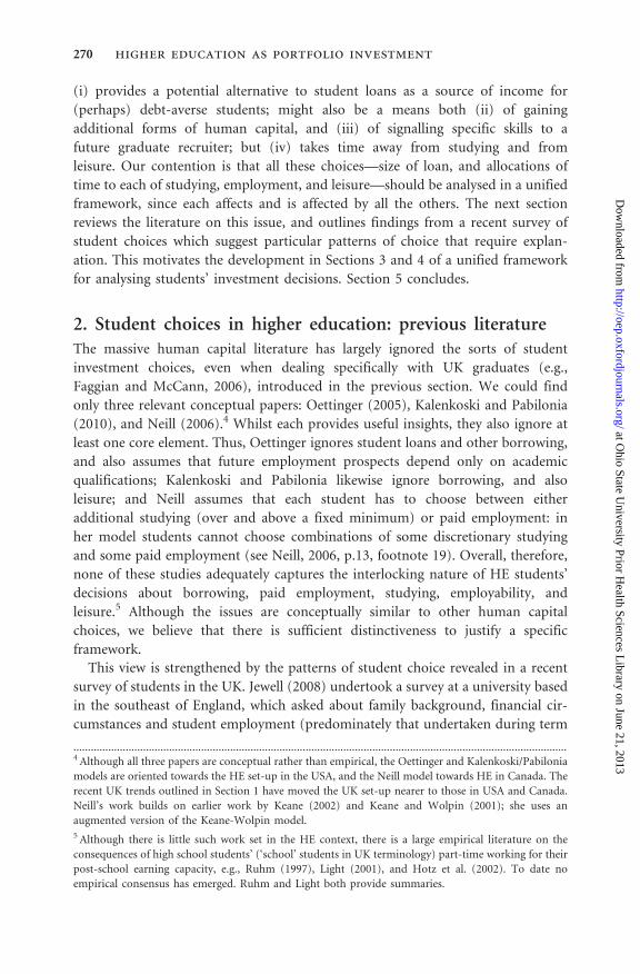
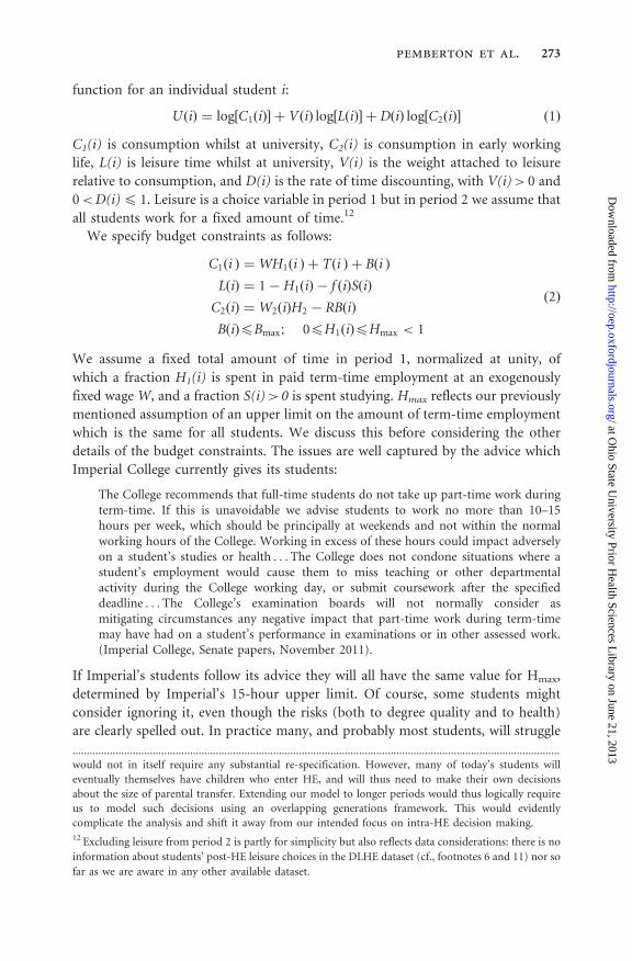
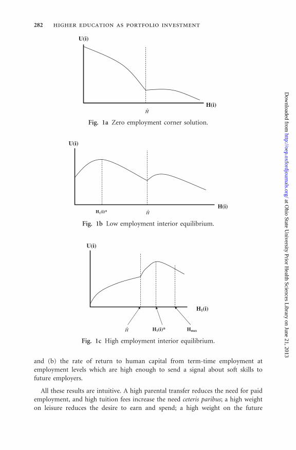
level yielding the highest utility. Figure 1 illustrates four possible forms for the
partial relationship between utility and term-time employment, each defining
a different optimal employment choice: corner solutions at H1* = 0 (Fig. 1a)
or at H1* = Hmax (Fig. 1d), and interior optima at low (Fig. 1b) or high (Fig. 1c)
employment.
Section 2 of the Appendix provides a detailed analysis which can be summarized
as follows:
Proposition 2 For a borrowing-constrained student the optimal term-time
employment level is decreasing in (i) the parental transfer; (ii) the utility weight
on leisure; (iii) the utility weight on the future; (iv) the utility-adjusted rate of
return to human capital from studying; (v) the rate of loan repayment; and (vi) the
size of the maximum available loan; and is increasing in (a) the level of tuition
fees (provided that the latter does not itself influence the maximum available loan);
..........................................................................................................................................................................21 Whereas Table 2 has four employment categories, Table 1 has five, corresponding to the definitions in
the Jewell (2008) dataset from which it is derived. We can think of Table 1’s ‘medium intensity’ category
as being subsumed into either the ‘low intensity’ or the ‘high intensity’ category for the purposes of
Table 2.
pemberton et al. 281
at Ohio State U
niversity Prior Health Sciences L
ibrary on June 21, 2013http://oep.oxfordjournals.org/
Dow
nloaded from
and (b) the rate of return to human capital from term-time employment at
employment levels which are high enough to send a signal about soft skills to
future employers.
All these results are intuitive. A high parental transfer reduces the need for paid
employment, and high tuition fees increase the need ceteris paribus; a high weight
on leisure reduces the desire to earn and spend; a high weight on the future
U(i)
H(i) H
Fig. 1a Zero employment corner solution.
U(i)
H1(i)* HH(i)
Fig. 1b Low employment interior equilibrium.
U(i)
H1(i)
H1(i)* H Hmax
Fig. 1c High employment interior equilibrium.
282 higher education as portfolio investment
at Ohio State U
niversity Prior Health Sciences L
ibrary on June 21, 2013http://oep.oxfordjournals.org/
Dow
nloaded from

incentivizes studying (whose pay-off is entirely in the future) relative to earning
(whose pay-off is partly in the present); a high rate of loan repayment (and
therefore, ceteris paribus, lower future spending) likewise incentivizes studying
over work in order to raise future income; and a high Bmax increases current
resources and reduces the need to earn. All these influences act to reduce
term-time employment; conversely, a high rate of return to future human capital
from term-time employment provides a direct incentive to work more.
The preceding discussion focuses on borrowing-constrained individuals. We
briefly consider the choice between Cases 5 and 7. In both cases B*<Bmax, and
in both cases employment is at a corner: H1* = 0 in Case 5, and H1* = Hmax in
Case 7. We proceed as in the Appendix, Section 2, by comparing the highest
attainable utility level in each case. Using the solutions for C1(i)*, C2(i)*, and
L(i)* in Table A2 it can be checked that utility in Case 5 is higher (lower) than
in Case 7 if C1(i)* is higher (lower) in Case 5 than in Case 7; and it is easily
established that this applies if X(i) (defined in Table A3) is positive (negative).
Using Table A3’s definition of X(i):
Proposition 3 The probability that a borrowing-unconstrained student will prefer
maximum to zero employment is increasing in the loan repayment rate and the rate
of return to human capital from term-time employment, and decreasing in the
utility-adjusted rate of return to human capital from studying.
Again these results are intuitive: a high loan repayment rate incentivizes employ-
ment and income earning in order to reduce the required size of loan; a high b(i)
directly incentivizes employment; and a high [a(i)/f(i)] incentivizes studying and
therefore disincentivizes alternative uses of time, including employment.
5. ConclusionsHigher education students face a pattern of incentives and constraints which
appears to push them systematically towards corner solutions rather than
U(i)
H1(i)
H Hmax
Fig. 1d Very high employment corner solution.
pemberton et al. 283
at Ohio State U
niversity Prior Health Sciences L
ibrary on June 21, 2013http://oep.oxfordjournals.org/
Dow
nloaded from

interior solutions for both their allocations of time and their levels of indebtedness.
We have formulated a framework which is consistent with this, and have used it to
derive results about students’ choices.
In conclusion we mention several implications and extensions of the analysis. At a
theoretical level, we have made various simplifications (e.g., all lending and
borrowing is at the same rate; the human capital eq. (3) is entirely additive; etc.)
and it would be useful to analyse to what extent relaxing these and other assumptions
would affect the results. At an empirical level, the paper develops many testable
predictions, and some of the underpinning assumptions (e.g., that the rate of
return on soft skills is always less than that on hard skills) are also testable. Finally,
the paper also identifies, but does not analyse, various public policy implications
which would merit further work. For example, an important issue both for public
policy and for universities is whether term-time working is a good or a bad thing. The
present paper analyses this only from the viewpoint of an individual student, but its
framework could be used to develop an analysis of the economy-wide social welfare
implications; and it also points towards policy levers that could be activated (either at
governmental level or by individual universities) either to encourage term-time
working (e.g., making it part of the formal curriculum), or to discourage it. In this
and other ways, the paper’s framework could be used as a starting point for analysing
the many important policy issues that stem from the expanding size and changing
nature of the higher education sector in the UK and elsewhere.
AcknowledgementsWe would like to thank two anonymous referees for their very helpful comments and
suggestions.
ReferencesBlanden, J. and Machin, S. (2004) Educational inequality and the expansion of higher
education, Scottish Journal of Political Economy, 51, 230–49.
Brown, P. and Hesketh, A. (2004) The Mismanagement of Talent, Oxford University Press,
Oxford.
Callender, C. and Kemp, M. (2000) Changing student finances: income, expenditure and the
take-up of student loans among full and part-time higher education students in 1998/99,
Research Report No. 213, Department for Education and Employment, London.
Callender, C. and Wilkinson, D. (2003) 2002/2003 Student income and expenditure survey:
students income’, expenditure and debt in 2002/2003 and changes since 1998/1999, Research
Report No. 487, Department for Education and Employment, Nottingham.
CBI (2009) Future fit: preparing graduates for the world of work, Confederation of British
Industry, London.
Deaton, A. (1991) Saving and liquidity constraints, Econometrica, 59, 1221–448.
Dickerson, A. and Green, F. (2004) The growth and valuation of computing and other
generic skills, Oxford Economic Papers, 56, 371–406.
284 higher education as portfolio investment
at Ohio State U
niversity Prior Health Sciences L
ibrary on June 21, 2013http://oep.oxfordjournals.org/
Dow
nloaded from

DIUS (2009) Participation rates in higher education academic years 1999/2000–2007/2008
(provisional), Department for Innovation, Universities and Skills, London.
Faggian, A. and McCann, P. (2006) Human capital and regional knowledge assets: a sim-
ultaneous equation model, Oxford Economic Papers, 58, 475–500.
Finch, S., Jones, A., Parfrement, J., Cebulla, A., Connor, H., Hillage, J., Pollard, E.,
Tyers, C., Hunt, W., and Loukas, G. (2006) Student income and expenditure survey
2004/05. Research Report No. 487, Department for Education and Employment, London.
Hotz, V., Lixin, C., Marta, T., and Avner, A. (2002) Are there returns to the wages of young
men from working while in school? Review of Economics and Statistics, 84, 221–36.
Jewell, S. (2008) Human capital acquisition and labour market outcomes in UK higher
education, PhD, School of Economics, University of Reading.
Jewell, S., Faggian, A., and King, Z. (2010) The effect of term-time employment on UK
higher education students, in L. Valencia and B. Hahn (eds) Employment and Labor Issues:
Unemployment, Youth Employment and Child Labor, Nova Science, Hauppage, NY.
Jones, R. and Sloane, P. (2005) Students and term-time employment, Report for The
Economic Research Unit, Welsh Assembly Government, University of Wales, Swansea.
Kalenkoskis, C. and Pabilonia, S. (2010) Parental transfers, student achievement, and the
labour supply of college students, Journal of Population Economics, 23, 469–96.
Keane, M. (2002) Financial aid, borrowing constraints and college attendance: evidence from
structural estimates, American Economic Review, Papers and Proceedings, 92, 293–97.
Keane, M. and Wolpin, K. (2001) The effect of parental transfers and borrowing constraints
on educational attainment, International Economic Review, 42, 1051–103.
Light, A. (2001) In-school work experience and the returns to schooling, Journal of Labor
Economics, 19, 65–93.
Neill, C. (2006) The effect of tuition fees on students’ work in Canada, unpublished
manuscript, Wilfrid Laurier University, Waterloo.
OECD (2009) Education at a Glance, 2009, OECD Publications, Paris.
Oettinger, G. (2005) Parents’ financial support, students’ employment, and academic per-
formance in college, unpublished manuscript, University Of Texas at Austin.
Purcell, K., Elias, P., Davies, R., and Wilton, N. (2005) The class of ’99: a study of the early
labour market experience of recent graduates, Report to the Department for Education and
Skills, London.
Purcell, K., Rowley, G., and Morley, M. (2002) Employers in the new graduate labour
market: recruiting from a wider spectrum of graduates, Council for Industry and Higher
Education, London.
Ruhm, C. (1997) Is high school employment consumption or investment? Journal of Labor
Economics, 15, 735–76.
TUC. (2006) All work and low pay: the growth in UK student employment, TUC, London.
Van Dyke, R., Little, B., and Callender, C. (2005) Survey of higher education students’
attitudes to debt and term time working and their impact on attainment, Higher
Education Funding Council for England, Bristol.
Zeldes, S. (1989) Consumption and liquidity constraints: an empirical investigation, Journal
of Political Economy, 97, 305–46.
pemberton et al. 285
at Ohio State U
niversity Prior Health Sciences L
ibrary on June 21, 2013http://oep.oxfordjournals.org/
Dow
nloaded from
Appendix
1. Borrowing choicesTable 2 indicates that B(i) = Bmax in five of the seven cases, and B(i)<Bmax in Cases
5 and 7. Hence we need to identify in what circumstances individuals will prefer
Cases 5 or 7 to any of the B = Bmax options. We begin with the choice between Cases
6 and 7. For Case 6 to be optimal requires both @UðiÞ=@H1ðiÞ � 0 in (4) and
@UðiÞ=@BðiÞ � 0 in (6) at the optimal values of C1(i)*, C2(i)*, and L(i)* given in
the relevant row of Table A2.22 Substituting these optimal values into (4) and (6)
allows the inequality conditions to be stated in terms of the size of the net financial
transfer T(i):
@UðiÞ
@H1ðiÞ� 0 if TðiÞ �
AðiÞ �WH2 aðiÞ � f ðiÞbðiÞ� �
Hmax þ f ðiÞbðiÞHh i
H2 aðiÞ � f ðiÞbðiÞ� �
DðiÞ þ VðiÞð Þ
� WHmax þ Bmaxð Þ � TðiÞ1
ðA1Þ
@UðiÞ
@BðiÞ� 0 if TðiÞ �
AðiÞ �WH2 aðiÞ � f ðiÞbðiÞ� �
Hmax þ f ðiÞbðiÞHh i
f ðiÞR DðiÞ þ VðiÞð Þ
� WHmax þ Bmaxð Þ � TðiÞ6
ðA2Þ
AðiÞ ¼ WH2 aðiÞ þ f ðiÞ� �
� f ðiÞRBmax ðA3Þ
Using (A1)–(A3) and the definition of ~RðiÞb in (9) indicates that
TðiÞ15 or � TðiÞ6 as R5 or � ~RðiÞb ðA4Þ
Noting from Table 2 that the choice between Cases 6 and 7 is only feasible for
Types 2 and 3, for both of whom R � ~RðiÞb, it follows that T(i)<T(i)6 is the
relevant condition for Case 6 to be preferred to Case 7. By implication Case 7
will be preferred if T(i)>T(i)6. This can be checked using Table A1’s specification
of Case 7’s optimal value of B(i)*: manipulating this expression indicates that the
requirement for it to be less than Bmax (as required in Case 7) is that T(i)>T(i)6.
Thus the choice between Cases 6 and 7 turns on the value of the net transfer T(i)
relative to the critical value T(i)6. This and subsequent results are summarized
in Table A3.
Equivalent considerations govern the choice between Cases 4 and 5, which
is feasible for Types 1 and 2 but not for Type 3. In both cases H1(i)* = 0, with
B(i)<Bmax in Case 5 and B(i) = Bmax in Case 4. To derive the condition governing
this choice we follow the same methodology as in (A1–A3): Case 4 requires
@UðiÞ=@BðiÞ � 0 in (6) at the optimal consumption and leisure values (specified
..........................................................................................................................................................................22 As explained earlier, C1(i)*, C2(i)* and L(i)* are obtained by substituting into the budget constraints
(2) the optimal values of H1(i)*, L(i)* and S(i)* obtained from (4)–(7). These optimal values incorporate
whichever corner solution[s] is/are appropriate to the case being considered. Thus, for Case 6 they
explicitly build in both the stated inequalities (and similarly for all the other cases discussed below.)
286 higher education as portfolio investment
at Ohio State U
niversity Prior Health Sciences L
ibrary on June 21, 2013http://oep.oxfordjournals.org/
Dow
nloaded from
in Table A2) which are applicable to Case 4, and some manipulation allows this
inequality to be re-written as T(i)<T(i)4, where T(i)4 is specified in Table A3.
Again proceeding as in the previous paragraph, it can be checked that if this
inequality is reversed Case 5 is then preferred instead.
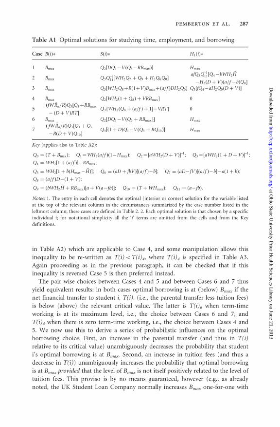
The pair-wise choices between Cases 4 and 5 and between Cases 6 and 7 thus
yield equivalent results: in both cases optimal borrowing is at (below) Bmax if the
net financial transfer to student i, T(i), (i.e., the parental transfer less tuition fees)
is below (above) the relevant critical value. The latter is T(i)6 when term-time
working is at its maximum level, i.e., the choice between Cases 6 and 7, and
T(i)4 when there is zero term-time working, i.e., the choice between Cases 4 and
5. We now use this to derive a series of probabilistic influences on the optimal
borrowing choice. First, an increase in the parental transfer (and thus in T(i)
relative to its critical value) unambiguously decreases the probability that student
i’s optimal borrowing is at Bmax. Second, an increase in tuition fees (and thus a
decrease in T(i)) unambiguously increases the probability that optimal borrowing
is at Bmax provided that the level of Bmax is not itself positively related to the level of
tuition fees. This proviso is by no means guaranteed, however (e.g., as already
noted, the UK Student Loan Company normally increases Bmax one-for-one with
Table A1 Optimal solutions for studying time, employment, and borrowing
Case BðiÞ� SðiÞ� H1ðiÞ�
1 Bmax Q2½DQ1�VðQ5�RBmaxÞ� Hmax
2 Bmax Q3Q�111½WH2Q7 þ Q9 þH2Q6Q0�
afQ3Q�111½Q4�bWH2H
�H2ðDþ VÞða=f �bÞQ0�
3 Bmax Q3½WH2Q8þRð1þVÞBmaxþða=f ÞDH2Q0� Q3½fQ4�aH2Q0ðDþ VÞ�
4 Bmax Q2½WH2ð1þQ8Þ þ VRBmax� 0
5ðfW ~Ra=RÞQ3½Q4þRBmax
� ðDþ VÞRT�Q3fWH2ðQ8 þ ða=f Þ þ 1��VRTg 0
6 Bmax Q2½DQ1�VðQ5 þ RBmaxÞ� Hmax
7ð fW ~Ra=RÞQ3½Q1 þQ5
�RðDþ VÞQ10�Q3½ð1þ DÞQ1�VðQ5 þ RQ10Þ� Hmax
Key (applies also to Table A2):
Q0 ¼ ðT þ BmaxÞ; Q1¼WH2ða=f Þð1�HmaxÞ; Q2¼½aWH2ðDþ VÞ��1; Q3¼½aWH2ð1þ Dþ VÞ��1;
Q4 ¼ WH2½1þ ða=f Þ��RBmax;
Q5 ¼ WH2½1þ bðHmax�HÞ�; Q6 ¼ ðaDþ fbVÞ½ða=f Þ�b�; Q7 ¼ ðaD�fVÞ½ða=f Þ�b��að1þ bÞ;
Q8 ¼ ða=f ÞD�ð1þ VÞ;
Q9 ¼ ðbWH2H þ RBmaxÞ½aþ Vða�fbÞ�; Q10 ¼ ðT þWHmaxÞ; Q11 ¼ ða�fbÞ:
Notes: 1. The entry in each cell denotes the optimal (interior or corner) solution for the variable listed
at the top of the relevant column in the circumstances summarized by the case number listed in the
leftmost column; these cases are defined in Table 2. 2. Each optimal solution is that chosen by a specific
individual i; for notational simplicity all the ‘i’ terms are omitted from the cells and from the Key
definitions.
pemberton et al. 287
at Ohio State U
niversity Prior Health Sciences L
ibrary on June 21, 2013http://oep.oxfordjournals.org/
Dow
nloaded from
tuition fees increases). Third, the probability that the net transfer T(i) is above its
critical value (so that B<Bmax) is decreasing (increasing) in parameters that
increase (decrease) whichever critical value, T(i)4 or T(i)6, is relevant. From
Table A3 both these critical values are decreasing in D(i), V(i), and R(i), and
increasing in [a(i)/f(i)]. In addition T(i)6 (but not T(i)4) is increasing in b(i).
Further, when B(i)*<Bmax (Cases 5 and 7) Table A1 indicates that B(i)* is
decreasing in T(i), V(i), D(i) and R(i) and increasing in a(i)/f(i) and (when
employment is at its maximum level, Case 7) is increasing in b(i). For appropriate
parameter combinations B(i)*< 0 is possible (i.e., net saving, and a zero student
loan). All the foregoing points are combined and summarized in Proposition 1
in Section 4.
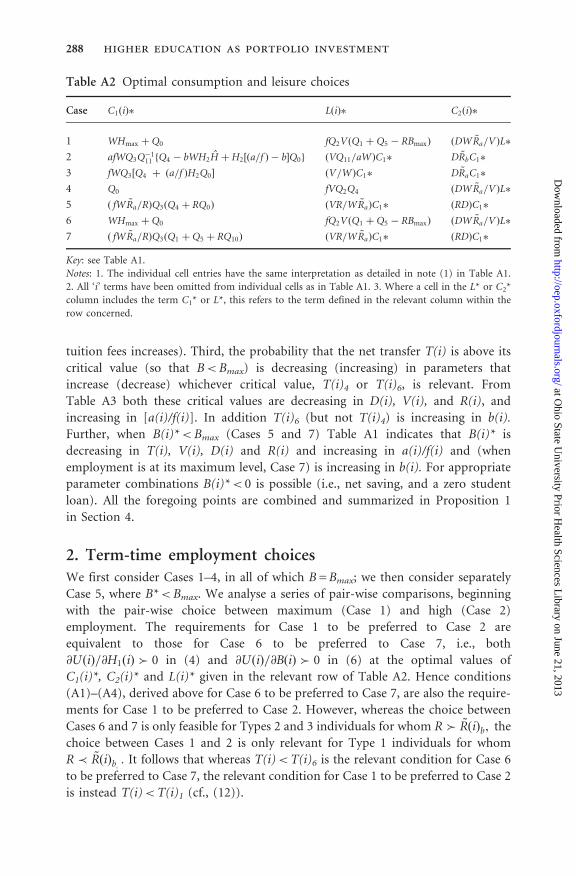
2. Term-time employment choicesWe first consider Cases 1–4, in all of which B = Bmax; we then consider separately
Case 5, where B*<Bmax. We analyse a series of pair-wise comparisons, beginning
with the pair-wise choice between maximum (Case 1) and high (Case 2)
employment. The requirements for Case 1 to be preferred to Case 2 are
equivalent to those for Case 6 to be preferred to Case 7, i.e., both
@UðiÞ=@H1ðiÞ � 0 in (4) and @UðiÞ=@BðiÞ � 0 in (6) at the optimal values of
C1(i)*, C2(i)* and L(i)* given in the relevant row of Table A2. Hence conditions
(A1)–(A4), derived above for Case 6 to be preferred to Case 7, are also the require-
ments for Case 1 to be preferred to Case 2. However, whereas the choice between
Cases 6 and 7 is only feasible for Types 2 and 3 individuals for whom R � ~RðiÞb, the
choice between Cases 1 and 2 is only relevant for Type 1 individuals for whom
R � ~RðiÞb, : It follows that whereas T(i)<T(i)6 is the relevant condition for Case 6
to be preferred to Case 7, the relevant condition for Case 1 to be preferred to Case 2
is instead T(i)<T(i)1 (cf., (12)).
Table A2 Optimal consumption and leisure choices
Case C1ðiÞ� LðiÞ� C2ðiÞ�
1 WHmax þ Q0 fQ2VðQ1 þ Q5 � RBmaxÞ ðDW ~Ra=VÞL�
2 afWQ3Q�111 fQ4 � bWH2H þH2½ða=f Þ � b�Q0g ðVQ11=aWÞC1� D ~RbC1�
3 fWQ3½Q4 þ ða=f ÞH2Q0� ðV=WÞC1� D ~RaC1�
4 Q0 fVQ2Q4 ðDW ~Ra=VÞL�
5 ð fW ~Ra=RÞQ3ðQ4 þ RQ0Þ ðVR=W ~RaÞC1� ðRDÞC1�
6 WHmax þ Q0 fQ2VðQ1 þ Q5 � RBmaxÞ ðDW ~Ra=VÞL�
7 ð fW ~Ra=RÞQ3ðQ1 þQ5 þ RQ10Þ ðVR=W ~RaÞC1� ðRDÞC1�
Key: see Table A1.
Notes: 1. The individual cell entries have the same interpretation as detailed in note (1) in Table A1.
2. All ‘i’ terms have been omitted from individual cells as in Table A1. 3. Where a cell in the L* or C2*
column includes the term C1* or L*, this refers to the term defined in the relevant column within the
row concerned.
288 higher education as portfolio investment
at Ohio State U
niversity Prior Health Sciences L
ibrary on June 21, 2013http://oep.oxfordjournals.org/
Dow
nloaded from
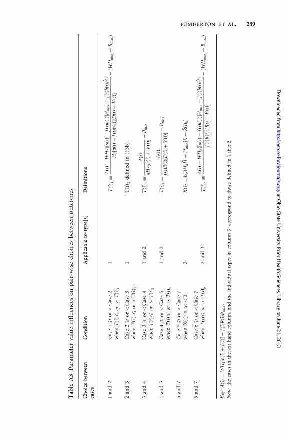
Tab
leA
3P
aram
eter
valu
ein
flu
ence
so
np
air-
wis
ech
oic
esb
etw
een
ou
tco
mes
Ch
oic
eb
etw
een
case
sC
on
dit
ion
Ap
pli
cab
leto
typ
e[s]
Def
init
ion
s
1an
d2
Cas
e15
or<
Cas
e2
1TðiÞ 1�
AðiÞ�
WH
2f½
aðiÞ�
fðiÞ
bðiÞ�H
maxþ
fðiÞ
bðiÞ
Hg
H2½aðiÞ�
fðiÞ
bðiÞ�½
DðiÞþ
VðiÞ�
�ðW
Hm
axþ
Bm
axÞ
wh
enTðiÞ4
or�
TðiÞ 1
2an
d3
Cas
e25
or<
Cas
e3
1T
(i) 2
def
ined
in(1
3b)
wh
enT
(i)4
or>
T(i
) 2
3an
d4
Cas
e35
or<
Cas
e4
1an
d2
TðiÞ 3�
AðiÞ
aH2½DðiÞþ
VðiÞ��
Bm
ax
wh
enTðiÞ4
or�
TðiÞ 3
4an
d5
Cas
e45
or<
Cas
e5
1an
d2
TðiÞ 4�
AðiÞ
fðiÞ
RðiÞ½
DðiÞþ
VðiÞ��
Bm
ax
wh
enTðiÞ4
or�
TðiÞ 4
5an
d7
Cas
e55
or<
Cas
e7
wh
enX
(i)5
or<
02
XðiÞ¼
bðiÞ
H2H�
Hm
ax½R�
~ RðiÞ b�
6an
d7
Cas
e65
or<
Cas
e7
wh
enTðiÞ4
or�
TðiÞ 6
2an
d3
TðiÞ 6�
AðiÞ�
WH
2f½
aðiÞ�
fðiÞ
bðiÞ�H
maxþ
fðiÞ
bðiÞ
Hg
fðiÞ
RðiÞ½
DðiÞþ
VðiÞ�
�ðW
Hm
axþ
Bm
axÞ
Key
:AðiÞ¼
WH
2½aðiÞþ
fðiÞ��
fðiÞ
RðiÞB
max
.
Not
e:th
eca
ses
inth
ele
fth
and
colu
mn
,an
dth
ein
div
idu
alty
pes
inco
lum
n3,
corr
esp
on
dto
tho
sed
efin
edin
Tab
le2.
pemberton et al. 289
at Ohio State U
niversity Prior Health Sciences L
ibrary on June 21, 2013http://oep.oxfordjournals.org/
Dow
nloaded from
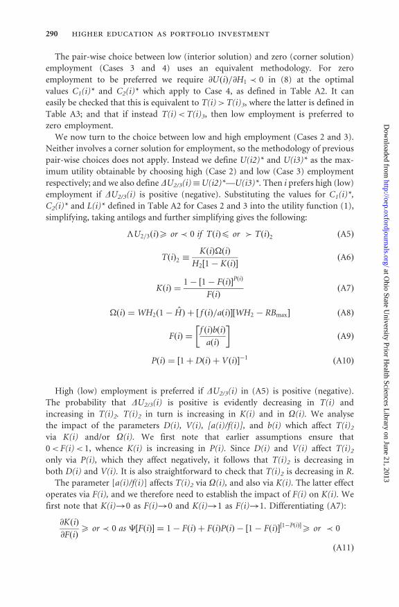
The pair-wise choice between low (interior solution) and zero (corner solution)
employment (Cases 3 and 4) uses an equivalent methodology. For zero
employment to be preferred we require @UðiÞ=@H1 � 0 in (8) at the optimal
values C1(i)* and C2(i)* which apply to Case 4, as defined in Table A2. It can
easily be checked that this is equivalent to T(i)>T(i)3, where the latter is defined in
Table A3; and that if instead T(i)<T(i)3, then low employment is preferred to
zero employment.
We now turn to the choice between low and high employment (Cases 2 and 3).
Neither involves a corner solution for employment, so the methodology of previous
pair-wise choices does not apply. Instead we define U(i2)* and U(i3)* as the max-
imum utility obtainable by choosing high (Case 2) and low (Case 3) employment
respectively; and we also define DU2/3(i)�U(i2)*—U(i3)*. Then i prefers high (low)
employment if DU2/3(i) is positive (negative). Substituting the values for C1(i)*,
C2(i)* and L(i)* defined in Table A2 for Cases 2 and 3 into the utility function (1),
simplifying, taking antilogs and further simplifying gives the following:
�U2=3ðiÞ5 or � 0 if TðiÞ4 or � TðiÞ2 ðA5Þ
TðiÞ2 �KðiÞ�ðiÞ
H2½1� KðiÞ�ðA6Þ
KðiÞ ¼1� 1� FðiÞ½ �
PðiÞ
FðiÞðA7Þ
�ðiÞ ¼ WH2ð1� HÞ þ ½ f ðiÞ=aðiÞ�½WH2 � RBmax� ðA8Þ
FðiÞ ¼f ðiÞbðiÞ
aðiÞ
� �ðA9Þ
PðiÞ ¼ 1þ DðiÞ þ VðiÞ½ ��1
ðA10Þ
High (low) employment is preferred if DU2/3(i) in (A5) is positive (negative).
The probability that DU2/3(i) is positive is evidently decreasing in T(i) and
increasing in T(i)2. T(i)2 in turn is increasing in K(i) and in O(i). We analyse
the impact of the parameters D(i), V(i), [a(i)/f(i)], and b(i) which affect T(i)2
via K(i) and/or O(i). We first note that earlier assumptions ensure that
0< F(i)< 1, whence K(i) is increasing in P(i). Since D(i) and V(i) affect T(i)2
only via P(i), which they affect negatively, it follows that T(i)2 is decreasing in
both D(i) and V(i). It is also straightforward to check that T(i)2 is decreasing in R.
The parameter [a(i)/f(i)] affects T(i)2 via O(i), and also via K(i). The latter effect
operates via F(i), and we therefore need to establish the impact of F(i) on K(i). We
first note that K(i)!0 as F(i)!0 and K(i)!1 as F(i)!1. Differentiating (A7):
@KðiÞ
@FðiÞ5 or � 0 as �½FðiÞ� ¼ 1� FðiÞ þ FðiÞPðiÞ � ½1� FðiÞ�½1�PðiÞ�5 or � 0
ðA11Þ
290 higher education as portfolio investment
at Ohio State U
niversity Prior Health Sciences L
ibrary on June 21, 2013http://oep.oxfordjournals.org/
Dow
nloaded from

Differentiating C[.]:
@�½FðiÞ�
@FðiÞ¼ ½1� PðiÞ�
1
1� FðiÞ½ �PðiÞ� 1
� �� 0 ðA12Þ
Using (A12) and noting that C[F(i)]!0 as F(i)!0 and that C[F(i)]!P(i)
[0<P(i)< 1] as F(i)!1, it follows that C[F(i)]>0 for all admissible values of
F(i) and hence, from (A11) that @KðiÞ=@FðiÞ � 0 unambiguously. Noting that
both F(i) and O(i) are decreasing in [a(i)/f(i)] we can now sign the impact of
the latter upon T(i)2 unambiguously:
dTðiÞ2
d aðiÞf ðiÞ
¼ @TðiÞ2@KðiÞ
� �@KðiÞ
@FðiÞ
� �@FðiÞ
@ aðiÞf ðiÞ
0@
1Aþ @TðiÞ2
@�ðiÞ
� �@�ðiÞ
@ aðiÞf ðiÞ
0@
1A � 0 ðA13Þ
Finally, noting that b(i) affects T(i)2 only via F(i) and that @FðiÞ=@bðiÞ�0, it follows
from the foregoing analysis that T(i)2 is increasing in b(i). Summarizing the
analysis of (A11)–(A13), T(i)2 is decreasing in D(i), V(i), R, and a(i)/f(i), and is
increasing in b(i). Feeding these results into (A5) in turn generates results
concerning the sign of DU2/3.
The discussion in this section has so far related to adjacent employment choices
(e.g., zero-low) rather than non-adjacent choices (e.g., zero-high). To derive global
results we note from Table A3 and (A6)–(A10) that T(i)1<T(i)3 unambiguously
but that T(i)2 can be larger or smaller than either or both. Using this and earlier
results allows us to identify three global patterns of choice for borrowing-
constrained individuals:
Pattern A T(i)2<T(i)1<T(i)3: zero employment is chosen if T(i)>T(i)3; low
employment if T(i)1<T(i)<T(i)3; either low or maximum employment if
T(i)2<T(i)<T(i)1; maximum employment if T(i)<T(i)2.
Pattern B T(i)1<T(i)2<T(i)3: zero employment is chosen if T(i)>T(i)3; low
employment if T(i)2<T(i)<T(i)3; high employment if T(i)1<T(i)<T(i)2;
maximum employment if T(i)<T(i)1.
Pattern C T(i)1<T(i)3<T(i)2: zero employment is chosen if T(i)>T(i)2;
either zero or high employment if T(i)3<T(i)<T(i)2; high employment if
T(i)1<T(i)<T(i)3; maximum employment if T(i)<T(i)1.
Pattern B identifies a straightforward inverse relationship between the net financial
transfer T(i) and the optimal employment category. Patterns A and C are similar,
but in each case one potential employment category is infeasible. All three patterns
replicate at a global level the relationships that we have identified from (A5)–(A13)
between adjacent employment levels. In particular, the employment category that is
optimal for any individual student is inversely related to her net transfer T(i); and
the probability that, for a given transfer, she is located in or below any given
employment category is positively related to the relevant T(i)N value (N = 1,2,3)
which determines its upper boundary point. The T(i)N values are themselves
pemberton et al. 291
at Ohio State U
niversity Prior Health Sciences L
ibrary on June 21, 2013http://oep.oxfordjournals.org/
Dow
nloaded from

determined by a series of independent parameters whose impact can be obtained by
differentiation of the T(i)N. To sign the impact of [a(i)/f(i)] we assume (WH2-
RBmax)>0, i.e., student loan repayments are never large enough to exhaust period 2
labour income even if the latter is not increased at all by human capital obtained
whilst at university. In differentiating T(i)2 in (A6) we make use of results derived
in (A11)–(A13). All the points listed so far in this paragraph relate to discrete
employment level categories, but two of these—the low and high employment
categories—encompass a range of possible employment levels, and contingent on
either category being optimal the precise employment level which is optimal within
the relevant range likewise depends on a series of independent parameters whose
effects can be determined by differentiating the appropriate expressions for H1(i)*
in Table (A1). Combining all these points together gives the results summarized in
Proposition 2 in Section 4.
292 higher education as portfolio investment
at Ohio State U
niversity Prior Health Sciences L
ibrary on June 21, 2013http://oep.oxfordjournals.org/
Dow
nloaded from
Top Related