


Languages
Pages
Legal


HIGH-MIXED-FREQUENCY
FORECASTING MODELS –
WITH APPLICATIONS TO
PHILIPPINE GDP AND
INFLATION
Roberto S. Mariano & Suleyman Ozmucur
University of Pennsylvania
SKBI Seminar, SMU, Singapore – November 23, 2018

SMU Classification: Restricted
INTRODUCTION
Main Topic: technical and practical issues involved
in the use of data at mixed and high frequencies
(quarterly and monthly and, possibly, weekly and
daily) to forecast monthly and quarterly economic
activity in a country
Renewed interest in this topic – for timely utilization
of high-frequency indicators to update market
assessments and forecasts – e.g.,
Government policy planners
Investors, industry & business leaders and
analysts2

SMU Classification: Restricted
INTRODUCTION (CONT)
Based on Mariano & Ozmucur, Chapter 1 in Peter Pauly
(editor) Global Economic Modeling. World Scientific, 2018
Consider high-frequency forecasting models for GDP growth
& inflation in the Philippines, focusing on
Multi-Frequency Dynamic Latent Factor Models (MF-DLFM) and
Mixed Data Sampling (MIDAS) Regression
Also consider alternative earlier approaches such as
AR and VAR benchmark models
Current Quarter Modeling (CQM) with Bridge Equations
3
SMU Classification: Restricted
PRACTICAL AND TECHNICAL
ISSUES
Timely and statistically efficient use of breaking “news” for
forecast updates --- so use mixed frequency data
(quarterly, monthly, weekly, daily, or even intra-day, like tick
data in the stock market)
Prefer data-parsimonious over data-intensive models
(without sacrificing forecast accuracy)
Combination of mixed-frequency data and latent factors in
the dynamic latent factor model introduces additional
complexities in the estimation and simulation of the model
Data reduction techniques are needed when dealing with a
large number of variables in the data set4
SMU Classification: Restricted
MIXED-FREQUENCY DATA SET
In general, the data set may include quarterly,
monthly, weekly, and daily observations
In this paper,
target variables – quarterly
GDP and GDP deflator, growth rates
indicator variables – monthly (more specific
details in subsequent slides)
5
SMU Classification: Restricted
ALTERNATIVE FORECASTING
MODELS (VIS-À-VIS FREQUENCY)
Quarterly Models
Use observed quarterly values of target variables
Aggregate over the quarter for the monthly indicators,
Average over the quarter for a stock variable
Sum for a flow variable
Calculate growth rates from the aggregated series
Monthly Models
Considers all the data series (target or indicator) as generated
at the highest frequency (monthly, in our case), but some of
them are not observed
Variables observed at the low frequency (quarterly) are treated
as having periodically missing or unobserved data points,
available only at the end month of the quarter6
SMU Classification: Restricted
QUARTERLY MODELS
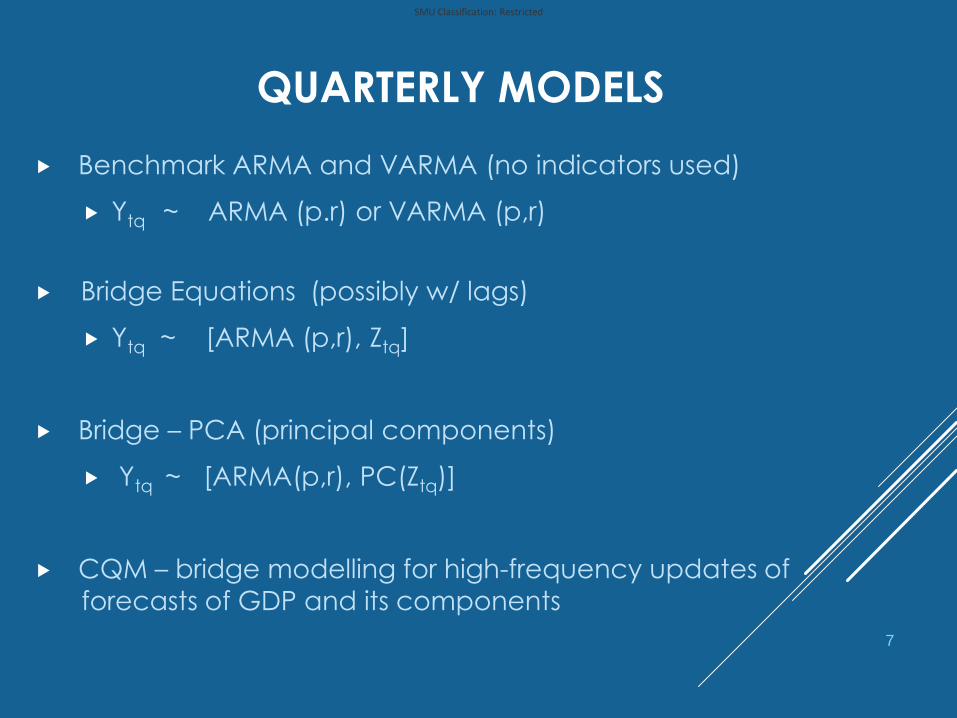
Benchmark ARMA and VARMA (no indicators used)
Ytq ~ ARMA (p.r) or VARMA (p,r)
Bridge Equations (possibly w/ lags)
Ytq ~ [ARMA (p,r), Ztq]
Bridge – PCA (principal components)
Ytq ~ [ARMA(p,r), PC(Ztq)]
CQM – bridge modelling for high-frequency updates of forecasts of GDP and its components
7

SMU Classification: Restricted
A BIT MORE ON CQM
Objective: timely forecast of GDP and its components in
the national income accounts, typically available quarterly
Use “bridge” equations, relating GDP components to
observabvle quarterly and monthly “indicator” variables.
Monthly observations are averaged over the quarter, with
updates as more monthly observations become available
To forecast the monthly and quarterly indicators, ARIMA
models are used
If no indicators are available, an ARIMA model would be
estimated for the GDP component itself
8

SMU Classification: Restricted
MONTHLY MODELS (HIGHEST FREQUENCY)
Mixed-Frequency Vector Autoregressive (MF-VAR)
Ytm ~ [VAR(p), Ztm)
Has a state-space model formulation
Can use Kalman filtering methods to estimate the model
and calculate forecasts at the highest frequency
Mixed Data Sampling (MIDAS) Regressions
Mixed Frequency Dynamic Latent Factor Model (MF-DLFM)
All these models also provide estimates and forecasts of the
target variables disaggregated at the high frequency
(monthly)
9
SMU Classification: Restricted
MIDAS
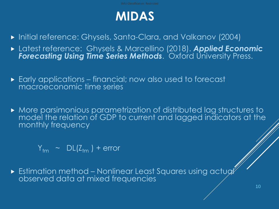
Initial reference: Ghysels, Santa-Clara, and Valkanov (2004)
Latest reference: Ghysels & Marcellino (2018). Applied Economic Forecasting Using Time Series Methods. Oxford University Press.
Early applications – financial; now also used to forecast macroeconomic time series
More parsimonious parametrization of distributed lag structures to model the relation of GDP to current and lagged indicators at the monthly frequency
Ytm ~ DL(Ztm ) + error
Estimation method – Nonlinear Least Squares using actual observed data at mixed frequencies
10

SMU Classification: Restricted
MIDAS (CONT) - LAG STRUCTURES
ΣKCK LK
(AVAILABLE IN EVIEWS 9.5)
Step Function (equal weights for months of same quarter, truncated)
Polynomial Almon Lag
Exponential Almon
ck = exp(θ1k + θ2k2)/ Σkexp(θ1k + θ2k
2)
Beta Lag ck = f(k/K;a,b) / Σk f(k/K;a,b),
f (x;a,b)= xa-1 (1-x)G(a+b)/[G(a)G(b)]
11
SMU Classification: Restricted
MIDAS (CONT)
SOME EXTENSIONS
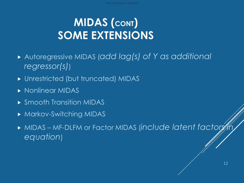
Autoregressive MIDAS (add lag(s) of Y as additional
regressor(s))
Unrestricted (but truncated) MIDAS
Nonlinear MIDAS
Smooth Transition MIDAS
Markov-Switching MIDAS
MIDAS – MF-DLFM or Factor MIDAS (include latent factors in
equation)
12
SMU Classification: Restricted
MIXED FREQUENCY DYNAMIC LATENT
FACTOR MODEL (MF-DLFM) –
ONE COMMON FACTOR
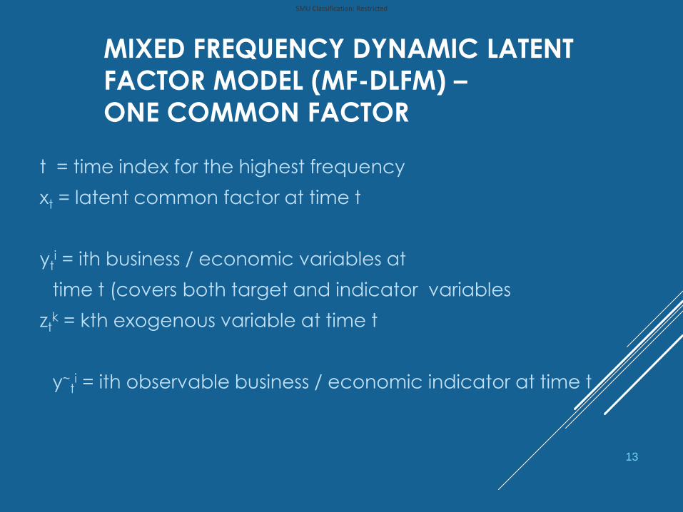
t = time index for the highest frequency
xt = latent common factor at time t
yti = ith business / economic variables at
time t (covers both target and indicator variables
ztk = kth exogenous variable at time t
y~ti = ith observable business / economic indicator at time t
13

SMU Classification: Restricted
MF-DLFM MODEL
1. Model for latent factor xt : AR(p) + error
r(L) xt = et, et ~ iid N(O,1) ,
r (L) = 1 + r L + r2L2 + … + rp Lp
2. Model for variables yti (NOT fully observed!)
yti = ci + bi xt + Sk(dik zt
k) + g(L) yti + ut
i
= [AR(r) , xt , zt ] + error
14
SMU Classification: Restricted
MF-DLFM
STATE SPACE FORMULATION
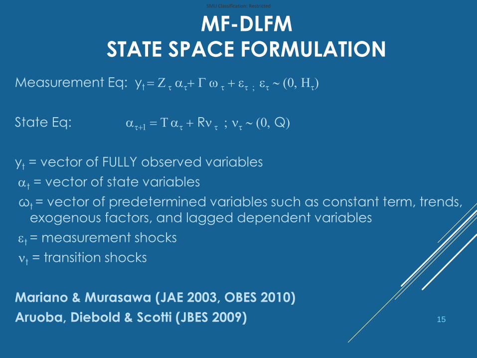
Measurement Eq: yt = Z t at+ G w t + et ; et ~ (0, Ht)
State Eq: at+1 = T at + Rn t ; nt ~ (0, Q)
yt = vector of FULLY observed variables
at = vector of state variables
ωt = vector of predetermined variables such as constant term, trends,
exogenous factors, and lagged dependent variables
et = measurement shocks
nt = transition shocks
Mariano & Murasawa (JAE 2003, OBES 2010)
Aruoba, Diebold & Scotti (JBES 2009) 15

SMU Classification: Restricted
EMPIRICAL RESULTS IN THE PAPER -
PHILIPPINES
Two Target Quarterly Variables
Real GDP Growth Rate
GDP Deflator Growth Rate
All Indicator Variables are monthly
Estimation Period
2000.Q1 – 2015.Q4
16
SMU Classification: Restricted
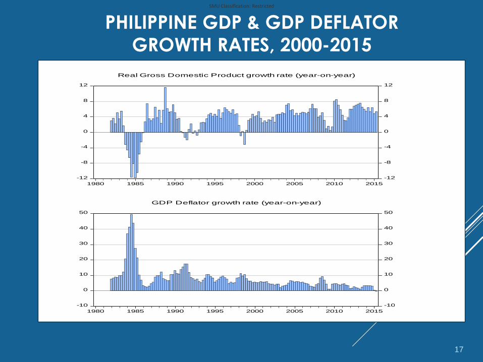
PHILIPPINE GDP & GDP DEFLATOR
GROWTH RATES, 2000-2015
-12
-8
-4
0
4
8
12
-12
-8
-4
0
4
8
12
1980 1985 1990 1995 2000 2005 2010 2015
Real Gross Domestic Product growth rate (year-on-year)
-10
0
10
20
30
40
50
-10
0
10
20
30
40
50
1980 1985 1990 1995 2000 2005 2010 2015
GDP Deflator growth rate (year-on-year)
17
SMU Classification: Restricted
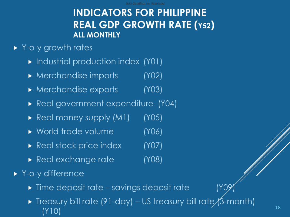
INDICATORS FOR PHILIPPINE
REAL GDP GROWTH RATE (Y52)ALL MONTHLY
Y-o-y growth rates
Industrial production index (Y01)
Merchandise imports (Y02)
Merchandise exports (Y03)
Real government expenditure (Y04)
Real money supply (M1) (Y05)
World trade volume (Y06)
Real stock price index (Y07)
Real exchange rate (Y08)
Y-o-y difference
Time deposit rate – savings deposit rate (Y09)
Treasury bill rate (91-day) – US treasury bill rate (3-month)
(Y10)18
SMU Classification: Restricted
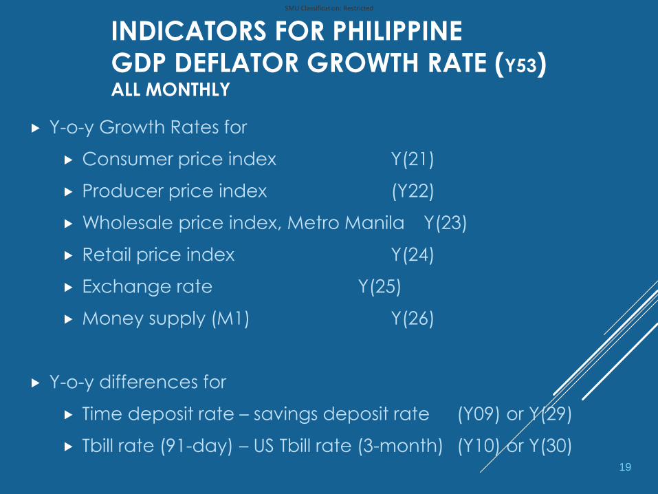
INDICATORS FOR PHILIPPINE
GDP DEFLATOR GROWTH RATE (Y53) ALL MONTHLY
Y-o-y Growth Rates for
Consumer price index Y(21)
Producer price index (Y22)
Wholesale price index, Metro Manila Y(23)
Retail price index Y(24)
Exchange rate Y(25)
Money supply (M1) Y(26)
Y-o-y differences for
Time deposit rate – savings deposit rate (Y09) or Y(29)
Tbill rate (91-day) – US Tbill rate (3-month) (Y10) or Y(30)19

SMU Classification: Restricted
FORECASTING MODELS
ESTIMATED FOR THE PHILIPPINES
Quarterly
AR
VAR
LEI
Bridge
Bridge – PCA
PCA with Two Groups
Monthly
MIDAS – polynomial Almon lag
MIDAS – PCA
MF-DLFM20

SMU Classification: Restricted
ESTIMATED BENCHMARK AND LEI
Estimated quarterly AR models:
AR(1) for real GDP growth rate, with R2 = 0.49
AR(2) for GDP deflator growth rate, R2 = 0.67
Estimated quarterly VAR for Y52 and Y53 : VAR(2)
LEI includes the leading economic indicator index and its lags
as additional regressors in the individual quarterly AR models.
Estimation results: ARDL(1,1) for real GDP and ARDL(2,0) for the
GDP deflator, with R2 = 0.58 and R2 = 0.67, respectively
21

SMU Classification: Restricted
ESTIMATED BRIDGE & BRIDGE-PCA
BRIDGE and BRIDGE-PCA equations are estimated separately for the two target variables. These are quarterly data regressions of target variables on the indicators, with monthly indicators converted to quarterly by averaging.
R2 values for the estimated Bridge equations
0.74 for real GDP growth
0.89 for GDP deflator growth
22
SMU Classification: Restricted
ESTIMATED MIDAS
MIDAS – regressions with Almon polynomial lags are estimated separately for the two target variables. For MIDAS-PCA principal components of the indicators are utilized in the regressions. Results for MIDAS-PCA are not much different from MIDAS; but there are some differences in forecasting performance
R2 values: 0.90 for real GDP; 0.95 for the GDP deflator
23
SMU Classification: Restricted
ESTIMATED MF-DLFM
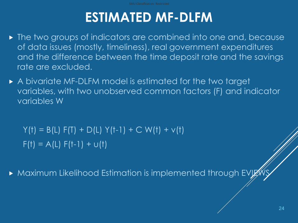
The two groups of indicators are combined into one and, because
of data issues (mostly, timeliness), real government expenditures
and the difference between the time deposit rate and the savings
rate are excluded.
A bivariate MF-DLFM model is estimated for the two target
variables, with two unobserved common factors (F) and indicator
variables W
Y(t) = B(L) F(T) + D(L) Y(t-1) + C W(t) + v(t)
F(t) = A(L) F(t-1) + u(t)
Maximum Likelihood Estimation is implemented through EVIEWS
24

SMU Classification: Restricted
MF-DLFM ONE-STEP AHEAD
FORECASTS – Y52 & Y53
25
-4
-2
0
2
4
0
2
4
6
8
10
2000 2002 2004 2006 2008 2010 2012 2014
One-step-ahead Y52
-4
-2
0
2
4
-4
0
4
8
12
2000 2002 2004 2006 2008 2010 2012 2014
One-step-ahead Y53
SMU Classification: Restricted
COMPARISON OF ERROR STATISTICS
Based on one-period-ahead forecasts, MF-DLFM has the lowest
mean absolute error and root mean square error for GDP growth rate - .40% for real GDP growth rate, and 0.33% for the nominal
GDP growth rate. Corresponding statistics are 0.43%, and 0.49%
for MIDAS_PCA, which ranks the second. Principal components,
and bridge equations follow these two models. The benchmark
AR and VAR models show the biggest errors.
On the other hand, MIDAS_PCA has the lowest mean absolute
error for the GDP deflator (0.34%). MF-DLFM, Bridge, and Bridge-
PCA MAEs are bunched at 0.47%. AR and VAR models show
the biggest errors.
26
SMU Classification: Restricted
27
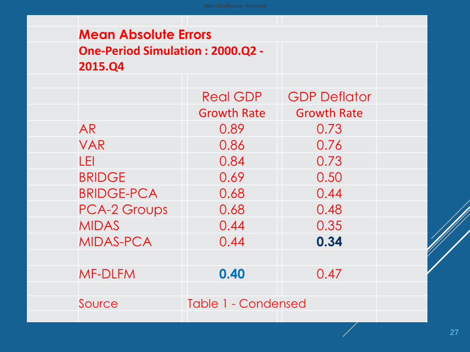
Mean Absolute Errors
One-Period Simulation : 2000.Q2 -2015.Q4
Real GDP GDP Deflator
Growth Rate Growth Rate
AR 0.89 0.73
VAR 0.86 0.76
LEI 0.84 0.73
BRIDGE 0.69 0.50
BRIDGE-PCA 0.68 0.44
PCA-2 Groups 0.68 0.48
MIDAS 0.44 0.35
MIDAS-PCA 0.44 0.34
MF-DLFM 0.40 0.47
Source Table 1 - Condensed
SMU Classification: Restricted
COMPARISON RESULTS FOR THE PHILIPPINES -
DIEBOLD-MARIANO TEST
Diebold-Mariano statistics were calculated to test the forecast
accuracy of MF-DLFM relative to the other models, one at a
time. For real GDP growth, test results show statistically
significant lower errors for MF-DLFM, except when compared
with MIDAS or MIDAS-PCA.
For the GDP deflator, the MIDAS-PCA average forecast error is
the lowest and significantly better than MF-DLFM at 5% critical
level.
MF-DLFM has lower errors relative to Bridge and Bridge-PCA,
but not statistically significant at 5%.
The bivariate tests done here can be extended to a
multivariate test comparing MF-DLFM with the alternative methods taken together - see Mariano & Preve (2012)
28

SMU Classification: Restricted
29
Diebold-Mariano Statistics for Forecast Accuracy
Alternative Model Versus MF-DLFM
Based on Squared Forecast Errors
Over 2000.Q2 - 2015.Q4
Real GDPGDP
Deflator
AR 2.45 3.05
VAR 4.02 3.23
LEI 2.74 3.04
BRIDGE 3.90 1.70
BRIDGE-PCA 3.92 0.35
PCA-2 Groups 3.92 1.40
MIDAS 0.96 -1.81
MIDAS-PCA 1.16 -2.07
Source Table 2 - Condensed

SMU Classification: Restricted
COMPARISON RESULTS FOR THE PHILIPPINES
– TURNING POINT ANALYSIS
All models do relatively well, if the prediction is for the level of
GDP, real GDP or the GDP deflator. However, not all of them fare
well in predicting the turning point in the growth rate of these
indicators .
For the growth rates, MF-DLFM appears to have a bigger edge
over the other models in predicting turning points
DLFM correctly predicts 87% of turning points in real GDP, while
MIDAS predicts 74% of them. The ratio is 79% for the bridge
equation model, and the PCA model.
MF-DLFM correctly predicts 89% of downturns, and 85% of upturns. Corresponding ratios for the MIDAS model are 74% and 68%. 30
SMU Classification: Restricted
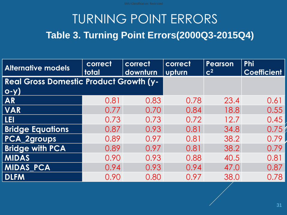
TURNING POINT ERRORS
Alternative modelscorrect total
correct downturn
correct upturn
Pearson c2
Phi Coefficient
Real Gross Domestic Product Growth (y-o-y)
AR 0.81 0.83 0.78 23.4 0.61
VAR 0.77 0.70 0.84 18.8 0.55
LEI 0.73 0.73 0.72 12.7 0.45
Bridge Equations 0.87 0.93 0.81 34.8 0.75
PCA_2groups 0.89 0.97 0.81 38.2 0.79
Bridge with PCA 0.89 0.97 0.81 38.2 0.79
MIDAS 0.90 0.93 0.88 40.5 0.81
MIDAS_PCA 0.94 0.93 0.94 47.0 0.87
DLFM 0.90 0.80 0.97 38.0 0.78
31
Table 3. Turning Point Errors(2000Q3-2015Q4)
SMU Classification: Restricted
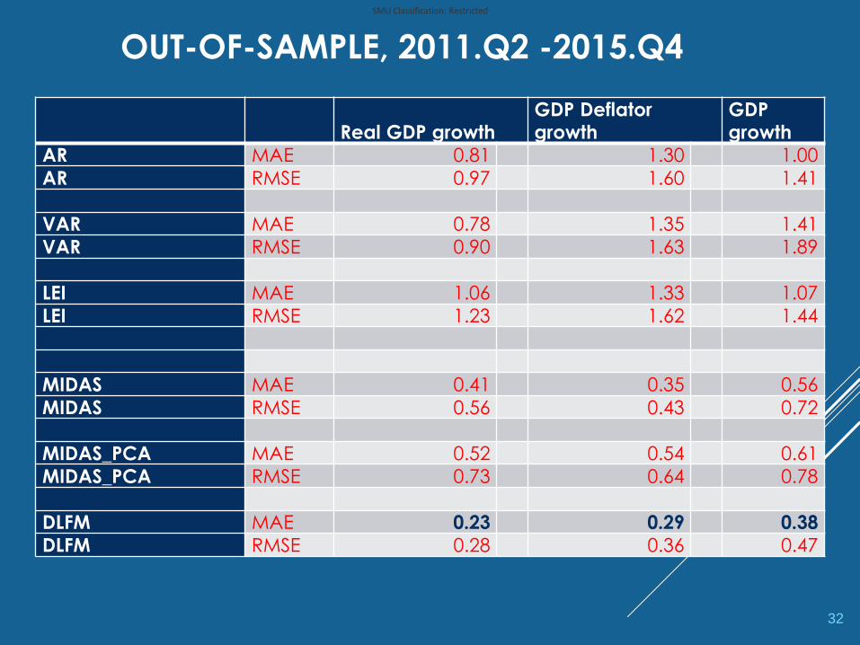
OUT-OF-SAMPLE, 2011.Q2 -2015.Q4
Real GDP growth GDP Deflator growth
GDP growth
AR MAE 0.81 1.30 1.00
AR RMSE 0.97 1.60 1.41
VAR MAE 0.78 1.35 1.41
VAR RMSE 0.90 1.63 1.89
LEI MAE 1.06 1.33 1.07
LEI RMSE 1.23 1.62 1.44
MIDAS MAE 0.41 0.35 0.56
MIDAS RMSE 0.56 0.43 0.72
MIDAS_PCA MAE 0.52 0.54 0.61
MIDAS_PCA RMSE 0.73 0.64 0.78
DLFM MAE 0.23 0.29 0.38
DLFM RMSE 0.28 0.36 0.47
32
SMU Classification: Restricted
CONCLUDING REMARKS
We have considered alternative models for use of data at
mixed frequencies (quarterly and monthly and, possibly, weekly
and daily) to forecast monthly and quarterly economic activity
in a country
While alternative models are mostly data-intensive, MF-DLFM
presents a parsimonious approach which depends on a much
smaller data set that needs to be updated regularly. But it also
faces additional complications in methodology and
calculations as mixed-frequency data are included in the
analysis.
33
SMU Classification: Restricted
CONCLUDING REMARKS
(CONT)MF-DLFM for real and nominal GDP
MIDAS for inflation
But final verdict is still on hold – more work needed – e.g.
more elaborate error structures
multiple latent common factors
choice of indicators
multiperiod forecasting (dynamic simulations)
how about other Asian countries?
34

THE END
Top Related