


Languages
Pages
Legal


Hierarchical Linear Models/Multilevel AnalysisEdps/Psych/Stat 587
Carolyn J. Anderson
Department of Educational Psychology
I L L I N O I Suniversity of illinois at urbana-champaign
Fall 2014

Introduction Data and Examples Applications Multilevel Theories & Propositions Summary
Overview
◮ Hierarchical Linear Models
◮ Multilevel Analysis using Linear Mixed Models
◮ Variance Components Analysis
◮ Random coefficients Models
◮ Growth curve analysis
All are special cases of Generalized Linear Mixed Models (GLMMs)
Reading:Snijders & Bosker (2012) — chapters 1 & 2
C.J. Anderson (Illinois) Introduction Fall 2014 2.1/ 53

Introduction Data and Examples Applications Multilevel Theories & Propositions Summary
Definition of Multilevel Analysis◮ Snijders & Bosker (2012):
Multilevel analysis is a methodology for the analysis ofdata with complex patterns of variability, with a focuson nested sources of variability.
◮ Wikipedia (Aug, 2014):
Multilevel models (also hierarchical linear models,nested models, mixed models, random coefficient,random-effects models, random parameter models, orsplit-plot designs) are statistical models of parametersthat vary at more than one level. These models canbe seen as generalizations of linear models (inparticular, linear regression), although they can alsoextend to non-linear models. These models becamemuch more popular after sufficient computing powerand software became available.[1]
◮ Today:
◮ Data and examples◮ Range of applications◮ Multilevel Theories
C.J. Anderson (Illinois) Introduction Fall 2014 3.1/ 53

Introduction Data and Examples Applications Multilevel Theories & Propositions Summary
Data and Examples
Children within families:
◮ Children with same biological parents tend to be more alikethan children chosen at random from the general population.
◮ They are more a like because
◮ Genetics◮ Environment◮ Both
C.J. Anderson (Illinois) Introduction Fall 2014 4.1/ 53
Introduction Data and Examples Applications Multilevel Theories & Propositions Summary
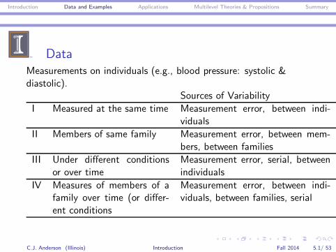
DataMeasurements on individuals (e.g., blood pressure: systolic &diastolic).
Sources of Variability
I Measured at the same time Measurement error, between indi-viduals
II Members of same family Measurement error, between mem-bers, between families
III Under different conditionsor over time
Measurement error, serial, betweenindividuals
IV Measures of members of afamily over time (or differ-ent conditions
Measurement error, between indi-viduals, between families, serial
C.J. Anderson (Illinois) Introduction Fall 2014 5.1/ 53

Introduction Data and Examples Applications Multilevel Theories & Propositions Summary
Examples of Hierarchies(a) Individuals within groups
Level 2
Level 1
Group 1
person11
���
person12
. . .person1n1
AAA
Group 2
person21
���
person22
. . .person2n2
AAA
. . . Group N
personN1
���
personN2
. . .personNnN
AAA
(b) LongitudinalLevel 2
Level 1
Person 1
time11
���
time12
. . .time1t1
AAA
Person 2
time21
���
time22
. . .time2t2
AAA
. . . Person N
timeN1
���
timeN2
. . .timeNtN
AAA
(c) Repeated Measures
Level 2
Level 1
Person 1
trial11
���
trial12
. . .trialn1
AAA
Person 2
trial1
���
trial2
. . .trialn2
AAA
. . . Person N
trialN1
���
trialN2
. . .trialNnN
AAA
C.J. Anderson (Illinois) Introduction Fall 2014 6.1/ 53

Introduction Data and Examples Applications Multilevel Theories & Propositions Summary
More Examples of Hierarchies
peer groups schools litters companies
kids students animals employees
neighborhoods schools clinics
families classes doctors
children students patients
C.J. Anderson (Illinois) Introduction Fall 2014 7.1/ 53

Introduction Data and Examples Applications Multilevel Theories & Propositions Summary
A Little Terminology
Hierarchy Levels Labels/terminology
Schools level 3 population, macro, primary units(first level sampled)
Classes level 2 sub-population, secondary units,groups
Students level 1 individuals, micro(last level sampled)
C.J. Anderson (Illinois) Introduction Fall 2014 8.1/ 53

Introduction Data and Examples Applications Multilevel Theories & Propositions Summary
Sampling Designs
Structure of data obtained by the way data are collected.
◮ Observational Studies.
◮ Experiments.
C.J. Anderson (Illinois) Introduction Fall 2014 9.1/ 53
Introduction Data and Examples Applications Multilevel Theories & Propositions Summary
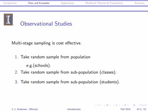
Observational Studies
Multi-stage sampling is cost effective.
1. Take random sample from population
e.g.(schools).
2. Take random sample from sub-population (classes).
3. Take random sample from sub-population (students).
C.J. Anderson (Illinois) Introduction Fall 2014 10.1/ 53
Introduction Data and Examples Applications Multilevel Theories & Propositions Summary
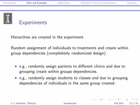
Experiments
Hierarchies are created in the experiment.
Random assignment of individuals to treatments and create withingroup dependencies (compleletely randomized design).
◮ e.g., randomly assign patients to different clinics and due togrouping create within groups dependencies.
◮ e.g., randomly assign students to classes and due to groupingdependencies of individuals in the same group created.
C.J. Anderson (Illinois) Introduction Fall 2014 11.1/ 53

Introduction Data and Examples Applications Multilevel Theories & Propositions Summary
Experiments (continue)
Grouping may initially be random but over the course of theexperiment individuals become differentiated.
◮ Groups =⇒ members.
◮ Members =⇒ groups.
C.J. Anderson (Illinois) Introduction Fall 2014 12.1/ 53

Introduction Data and Examples Applications Multilevel Theories & Propositions Summary
Analysis Must Incorporated Structure
Need to take structure of data into account because
◮ Invalidates most traditional statistical analysis methods (i.e.,independent observations).
◮ Risk overlooking important group effects.
◮ Within group dependencies is interesting phenomenon.
People exist within social contexts and want to study and makeinferences about individuals, groups, and the interplay betweenthem.
C.J. Anderson (Illinois) Introduction Fall 2014 13.1/ 53

Introduction Data and Examples Applications Multilevel Theories & Propositions Summary
Classic Example
◮ Bennett (1976): Statistically significant difference betweenways of teaching reading (i.e., “formal” styles are better thanothers).
◮ Data analyzed using traditional multiple regression wherestudents were the units of analysis.
◮ Atikin et al (’81): When the grouping of children into classeswas accounted for, significant differences disappeared.
C.J. Anderson (Illinois) Introduction Fall 2014 14.1/ 53

Introduction Data and Examples Applications Multilevel Theories & Propositions Summary
References
◮ Aitkin, M, Anderson, D, & Hinde, J. (1981). Statisticalmodelling of data on teaching styles. Journal of the RoyalStatistical Society, A, 144, 419-461.
◮ Aitkin, M., & Longford, N. (1986). Statistical modeling issuesin school effectiveness studies. Journal of the Royal StatisticalSociety, A, 149, 1-43. (with discussion).
◮ Goldstein, H. (1995). Multilevel statistical models, 2ndEdition. London: Arnold.
C.J. Anderson (Illinois) Introduction Fall 2014 15.1/ 53

Introduction Data and Examples Applications Multilevel Theories & Propositions Summary
What happened?
◮ Children w/in a classroom tended to be more similar withrespect to their performance.
◮ Each child provides less information than would have been thecase if they were taught separately.
◮ Teacher should have been the unit of comparison.
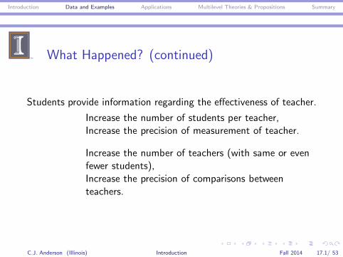
◮ Students provide information regarding the effectiveness ofteacher.
C.J. Anderson (Illinois) Introduction Fall 2014 16.1/ 53
Introduction Data and Examples Applications Multilevel Theories & Propositions Summary
What Happened? (continued)
Students provide information regarding the effectiveness of teacher.
Increase the number of students per teacher,Increase the precision of measurement of teacher.
Increase the number of teachers (with same or evenfewer students),Increase the precision of comparisons betweenteachers.
C.J. Anderson (Illinois) Introduction Fall 2014 17.1/ 53

Introduction Data and Examples Applications Multilevel Theories & Propositions Summary
Unit of Analysis Problem
◮ Problems with ignoring hierarchical structure of data were wellunderstood, but until recently, they were difficult to solve.
◮ Solution: Hierarchial linear models, along with computersoftware.
Hierarchical linear models are
◮ Generalizations of traditional linear regression models.
◮ Special cases of them include random and mixed effectsANOVA and ANCOVA models.
C.J. Anderson (Illinois) Introduction Fall 2014 18.1/ 53
Introduction Data and Examples Applications Multilevel Theories & Propositions Summary
A Little Example: NELS88 data
National Education Longitudinal Study — conducted by NationalCenter for Education Statistics of the US department of Education.
◮ Data constitute the first in a series of longitudinalmeasurements of students starting in 8th grade. Data werecollected Spring 1988.
◮ I obtained the data used here fromwww.stat.ucla.edu/∼deleeuw/sagebook
◮ From these data, we’ll use 2 out of the 1003 schools.
C.J. Anderson (Illinois) Introduction Fall 2014 19.1/ 53

Introduction Data and Examples Applications Multilevel Theories & Propositions Summary
NELS88: Data from two schools
C.J. Anderson (Illinois) Introduction Fall 2014 20.1/ 53

Introduction Data and Examples Applications Multilevel Theories & Propositions Summary
Schools 24725 and 62821 identified
C.J. Anderson (Illinois) Introduction Fall 2014 21.1/ 53

Introduction Data and Examples Applications Multilevel Theories & Propositions Summary
Applications of Multilevel Models
An incomplete list of possibilities:
Sample survey Measurement errorSchool/teacher effectiveness MultivariateLongitudinal Structural EquationDiscrete responses Event historyRandom cross-classifications Nonlinear patternsMeta Analysis IRT Models
C.J. Anderson (Illinois) Introduction Fall 2014 22.1/ 53

Introduction Data and Examples Applications Multilevel Theories & Propositions Summary
Survey Samples
Multi-stage sampling often used to collect data.
geographical area (clustering of polticial attitudes)
neighborhoods (clustering of SES)
households
“Nuisance factor”
The population structure is not interesting. So, multilevel samplingis a way to collect and analyze data about higher level units.
C.J. Anderson (Illinois) Introduction Fall 2014 23.1/ 53

Introduction Data and Examples Applications Multilevel Theories & Propositions Summary
School (teacher) Effectiveness
Students nested within schools.
◮ 1995 special issue Journal of Educational and BehavioralStatistic, 20 (summer) on Hierarchical Linear Models:Problems and Prospects.
◮ Educational researchers interested in comparing schools w/rtstudent performance (measured by standardized achievementtests).
◮ Public accountability.
◮ What factors explain differences between schools.
C.J. Anderson (Illinois) Introduction Fall 2014 24.1/ 53
Introduction Data and Examples Applications Multilevel Theories & Propositions Summary
Examples
Question: Does keeping gifted students in class or separate classeslead to better performance?
Measures available: Performance at beginning of year, performanceat end of year, and aptitude.
Question: To what extent do differences in average exam resultsbetween schools accounted for by factors such as
◮ Organizational practices
◮ Characteristics of students
C.J. Anderson (Illinois) Introduction Fall 2014 25.1/ 53

Introduction Data and Examples Applications Multilevel Theories & Propositions Summary
Advantages of multilevel approach
◮ Statistically efficient estimates of regression coefficients.
◮ Correct standard errors, confidence intervals, and significancetests.
◮ Can use covariates measured at any of the levels of thehierarchy.
C.J. Anderson (Illinois) Introduction Fall 2014 26.1/ 53

Introduction Data and Examples Applications Multilevel Theories & Propositions Summary
Example with Data
Rank schools w/rt to quality (adjusting for factors such as student“intake”)
Data: http://multilevel.ioe.ac.uk/
“The data come from the Junior School Project (Mortimore et al,1988). There are over 1000 students measured over three schoolyears with 3236 records included in this data set. Ravens test inyear 1 is an ability measure.”
C.J. Anderson (Illinois) Introduction Fall 2014 27.1/ 53

Introduction Data and Examples Applications Multilevel Theories & Propositions Summary
JSP Data:Columns Description Coding
1-2 School Codes from 1 to 5014-15 Mathematics test Score 1-4016 Junior school year One=0; Two=1;
Three=2
Goldstein,H. (1987). Multilevel Models in Educationaland Social Research. London, Griffin; New York, OxfordUniversity Press.1
Mortimore,P.,Sammons,P.,Stoll,L.,Lewis,D. & Ecob,R.(1988). School Matters, the Junior Years. Wells, OpenBooks.Prosser,R., Rasbash,J., and Goldstein,H.(1991). ML3Software for Three-level Analysis, Users’ Guide for V.2,Institute of Education, University of London.
1The data used by Goldstein consist of measures on 728 students in 50
elementary schools in inner London on two measurement occasions.C.J. Anderson (Illinois) Introduction Fall 2014 28.1/ 53

Introduction Data and Examples Applications Multilevel Theories & Propositions Summary
JSP: Level 1 Within School #1 Variation(R2 = .70)
C.J. Anderson (Illinois) Introduction Fall 2014 29.1/ 53

Introduction Data and Examples Applications Multilevel Theories & Propositions Summary
JSP: Level 2 Between School VariationMost R2’s between .6 and .9.
Different slopes and intercepts.C.J. Anderson (Illinois) Introduction Fall 2014 30.1/ 53

Introduction Data and Examples Applications Multilevel Theories & Propositions Summary
School/Teacher Effectiveness
May be OK to fit separate regressions, if
◮ Only a few schools each with a large number
of students
◮ Only want to make inferences about these specific schools.
However, if view schools as random sample from a large populationof schools, then need multilevel approach.
C.J. Anderson (Illinois) Introduction Fall 2014 31.1/ 53
Introduction Data and Examples Applications Multilevel Theories & Propositions Summary
Longitudinal Data
Same individuals measured on multiple occasions.
Individual
Occasions
◮ Strong hierarchies.
◮ Much more variations between individuals than betweenoccasions within individuals.
C.J. Anderson (Illinois) Introduction Fall 2014 32.1/ 53

Introduction Data and Examples Applications Multilevel Theories & Propositions Summary
A Little (hypothetical) Example
◮ Response variable: reading ability◮ Explanatory variable: Age◮ Two measurement occasions
C.J. Anderson (Illinois) Introduction Fall 2014 33.1/ 53

Introduction Data and Examples Applications Multilevel Theories & Propositions Summary
Hypothetical Example
Any explanations?C.J. Anderson (Illinois) Introduction Fall 2014 34.1/ 53

Introduction Data and Examples Applications Multilevel Theories & Propositions Summary
Longitudinal (continued)
◮ Traditional procedures:
◮ Balanced designs (no missing data)◮ All measurement occasions the same for all individuals.
◮ Multilevel modeling allows:
◮ Different occasions for different individuals.◮ Different number of observations per individual.◮ Build in particular error structures within individuals (eg,
auto-correlated errors).◮ Others....later
C.J. Anderson (Illinois) Introduction Fall 2014 35.1/ 53

Introduction Data and Examples Applications Multilevel Theories & Propositions Summary
Discrete Response Data
The response dependent variables are discrete rather thancontinuous.
◮ School’s exam pass rate (proportions).
◮ Graduation rate as a function of ethnic class.
◮ Rate of arrest from 911 calls.
Generalized linear mixed models (SAS procedures NLMIXED,GLMMIX, MDC, MCMC).
Some common IRT models are generalized non-linear mixedmodels (e.g., Rasch, 2PL, others).
C.J. Anderson (Illinois) Introduction Fall 2014 36.1/ 53

Introduction Data and Examples Applications Multilevel Theories & Propositions Summary
Multivariate Data
This is a variation of the use of hierarchical linear models foranalyzing longitudinal data.
individualւ ւ ց
x1 x2 . . . xp
Here we can have different variables and not every individual needsto have been measured on all of the variables...
C.J. Anderson (Illinois) Introduction Fall 2014 37.1/ 53

Introduction Data and Examples Applications Multilevel Theories & Propositions Summary
Nonlinear Models
Nonlinear models that are not linear in the parameters (e.g.,multiplicative).
Some kinds of growth models.
e.g., Growth spurts in children and when reach adulthood, growthlevels off.
Some nonlinear patterns can be modeled by polynomials or splines,but not all (e.g., logistic, discontinuous).
C.J. Anderson (Illinois) Introduction Fall 2014 38.1/ 53

Introduction Data and Examples Applications Multilevel Theories & Propositions Summary
Random cross-classifications
Subject X Stimuliց ւ
trial
elementary school X high schoolց ւ
individual
Raudenbush, S.W. (1993). A crossed random effects model forunbalanced data with applications in cross-sectional andlongitudinal research. Journal of Educational Statistics, 18,321–350.C.J. Anderson (Illinois) Introduction Fall 2014 39.1/ 53

Introduction Data and Examples Applications Multilevel Theories & Propositions Summary
Structural Equation ModelingIncluding Factor analysis
group
individualւ ց
item1 . . . item20
If apply factor analysis to responses from group data, the resultingfactors could represent
◮ Group differences
◮ Individual differences
C.J. Anderson (Illinois) Introduction Fall 2014 40.1/ 53

Introduction Data and Examples Applications Multilevel Theories & Propositions Summary
Measurement Error
. . . in the explanatory variables at different levels.
e.g. Let Yij be measure on individual i within group/cluster j andx∗ij be an explanatory variable measured with error.
Yij = βo + β1x∗
ij + ǫij
= βo + β1(xi + uj) + ǫij
= (βo + β1uj) + β1xi + ǫij
= β∗
oj + β1xi + ǫij
See also Muthen & Asparouhov (2011) who take a latent variableapproach.
C.J. Anderson (Illinois) Introduction Fall 2014 41.1/ 53

Introduction Data and Examples Applications Multilevel Theories & Propositions Summary
Other Applications
◮ Image analysis (e.g., analysis of shapes, DNA patterns,computer scans).
◮ How is repeated measures different from longitudinal?
◮ How could you do a meta-analysis as a multilevel (HLM)analysis?
◮ For some examples of these, seehttp://www.dartmouth.edu/∼eugened (Demidenko, EugeneMixed Models: Theory and Applications. NY: Wiley).
C.J. Anderson (Illinois) Introduction Fall 2014 42.1/ 53

Introduction Data and Examples Applications Multilevel Theories & Propositions Summary
Multilevel Theories and Propositions
From Snijders & Bosker
Handy device:
Macro-level Z marco in capital letters. . . ց. . . . . .
Micro-level x → y micro in lower case
C.J. Anderson (Illinois) Introduction Fall 2014 43.1/ 53

Introduction Data and Examples Applications Multilevel Theories & Propositions Summary
Micro-level propositions
No variables as the macro-level.Dependency is a nuisance.
. . . . . . . . .x → y
e.g., At macro-level you’ve randomly sampled towns and withintowns households.
x =occupational status,y =income
C.J. Anderson (Illinois) Introduction Fall 2014 44.1/ 53
Introduction Data and Examples Applications Multilevel Theories & Propositions Summary
Macro-level propositionsZ → Y. . . . . . . . .
Z and Y are not directly observable, but are composites (averages,aggregates) of micro-level measurements, then we end up withmultilevel structure.
e.g., Z = wealth of area (average SES).Y = school performance (mean achievement test).
lower mean SES → lower mean achievement test scores. or Z =
student/teacher ratio.
C.J. Anderson (Illinois) Introduction Fall 2014 45.1/ 53
Introduction Data and Examples Applications Multilevel Theories & Propositions Summary
Macro-Micro relations
Three basic possibilities:
◮ 1. Macro to micro.
◮ 2. Macro and micro to micro.
◮ 3. Macro–micro interaction.
C.J. Anderson (Illinois) Introduction Fall 2014 46.1/ 53

Introduction Data and Examples Applications Multilevel Theories & Propositions Summary
1. Macro to Micro.
Z. . . ց. . . . . .
y
y = math achievementZ = mean SES of students
Theory/proposition:
Higher average SES → higher math achievement
C.J. Anderson (Illinois) Introduction Fall 2014 47.1/ 53

Introduction Data and Examples Applications Multilevel Theories & Propositions Summary
2. Macro and Micro to MicroZ. . . ց. . . . . .x → y
x = # of hours spent doing homework.
Theory/proposition:
◮ Given time spent doing homework, higher average SES →
higher math achievement.
◮ Given average SES, more time spent doing homework →
higher math achievement.
C.J. Anderson (Illinois) Introduction Fall 2014 48.1/ 53

Introduction Data and Examples Applications Multilevel Theories & Propositions Summary
3. Macro-Micro Interaction
In the two macro-micro relations above, there is essentially achange in mean (random intercept). Here the relationship betweenx and y depends on Z .
Z. . . ↓. . . . . .x → y
Z = no/ability grouping of children,
x = aptitude or IQ, and y = achievement.
Theory: Small effect of x when there is grouping but large effectwhen there is no grouping.
C.J. Anderson (Illinois) Introduction Fall 2014 49.1/ 53

Introduction Data and Examples Applications Multilevel Theories & Propositions Summary
Emergent or micro-macro propositions
Z. . . ր. . . . . .x
Z = teacher’s experience of stress.x = student achievement.
C.J. Anderson (Illinois) Introduction Fall 2014 50.1/ 53

Introduction Data and Examples Applications Multilevel Theories & Propositions Summary
Another Example of Emergent
W Z. . . ց. . . . . .ր. . . . . .
x → y
W = teacher’s attitude toward learning.x = student’s attitude toward learning.y = student achievement.Z = teacher’s prestige.
C.J. Anderson (Illinois) Introduction Fall 2014 51.1/ 53

Introduction Data and Examples Applications Multilevel Theories & Propositions Summary
Summary
Clustered/multilevel/hierarchically structured data are assumed tobe
1. Random sample of macro-level units from population ofmacro-level units (or a representative sample).
2. Random sample of micro-level units from population of a(sampled) macro-level unit (or a representative sample).
C.J. Anderson (Illinois) Introduction Fall 2014 52.1/ 53

Introduction Data and Examples Applications Multilevel Theories & Propositions Summary
Advantages of multilevel approach
◮ Takes care of dependencies in data and gives correct standarderrors, confidence intervals, and significance tests.
◮ Statistically efficient estimates of regression coefficients.
◮ With clustered/multilevel/hierarchially structured data, canuse covariates measured at any of the levels of the hierarchy.
◮ Model all levels simultaneously.
◮ Study contextual effects.
◮ Theories can be rich.
However,
◮ Need to modify tools used in normal linear regression.
◮ Models can become overwhelmingly complex.
◮ Estimation can be a problem.
C.J. Anderson (Illinois) Introduction Fall 2014 53.1/ 53
Top Related