


Languages
Pages
Legal


Hidden Markov Models: Hidden Markov Models: an Introductionan Introduction
by Rachel Karchin
OutlineOutline
Stochastic ModelingDiscrete time seriesSimple Markov modelsHidden Markov modelsSummary of key HMM algorithmsModeling protein families with linear
profile HMMs

OutlineOutline
Overfitting and regularization.To come.

BME100 9/28/01
ReferencesReferences
Lectures from David Haussler’s CMPS243 class (Winter 1998)

BME100 9/28/01
Stochastic ModelingStochastic Modeling
Stochastic modeling. For phenomenon that exhibit random behavior.
Random doesn’t mean arbitrary. Random events can be modeled by some
probability distribution. Represented with random variables that
take on values (numeric or symbolic) according to event outcomes.

BME100 9/28/01
General Discrete Time SeriesGeneral Discrete Time Series
Chain of random variablesX1,X2,X3, . . . , Xn
Sequence of observed values x=x1,x2,x3, . . . , xn
When we observe x, say that: X1= x1,X2= x2,X3= x3, . . . , Xn= xn
BME100 9/28/01
Simple Markov model of order kSimple Markov model of order k
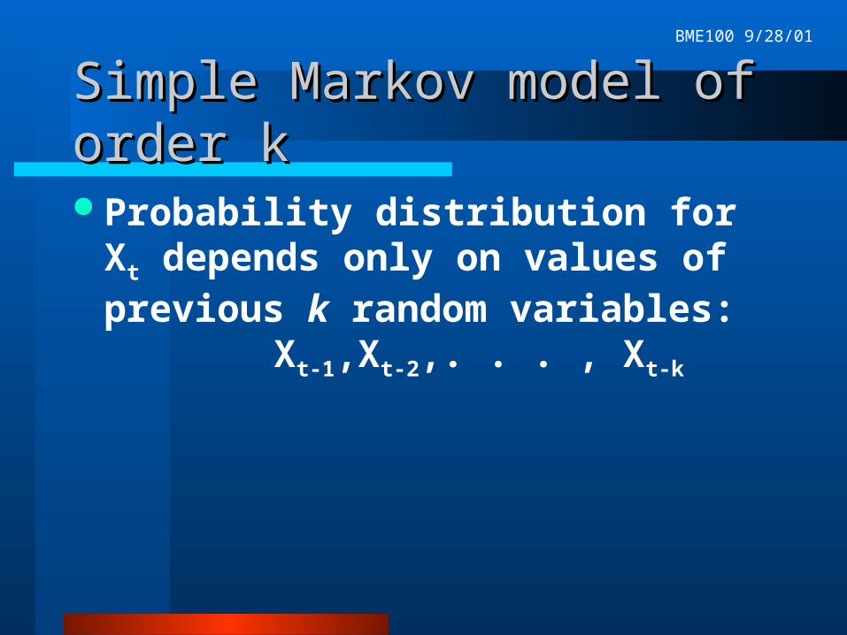
Probability distribution for Xt depends only on values of previous k random variables:
Xt-1,Xt-2,. . . , Xt-k

BME100 9/28/01
Simple Markov model of order kSimple Markov model of order k
Example with k=1 and Xt = {a,b}
Observed sequence: x = abaaababbaa
Model: Prev Next Prob
a 0.5 b 0.5
SStart probs
a a 0.7
a b 0.3
b a 0.5
b b 0.5
P(x) = 0.5 * 0.3* 0.5 * 0.7* 0.7 * 0.3 * 0.5 * 0.3 * 0.5 * 0.5 * 0.7

BME100 9/28/01
What is a hidden Markov model?What is a hidden Markov model?
Finite set of hidden states.At each time t, the system is in a hidden state, chosen at random depending on
state chosen at time t-1.At each time t, observed letter is generated at random, depending only on
current hidden state.

BME100 9/28/01
HMM for random toss of fair and HMM for random toss of fair and biased coinsbiased coins
0.8
0.2
0.2
0.8P(H)=0.
5
P(T)=0.5
FairP(H)=0.
1
P(T)=0.9
Biased
Start 0.5
0.5
Sequence of states: q = FFFFBBBFFFFFObserved sequence: x = HTTHTTTTHHTH
BME100 9/28/01
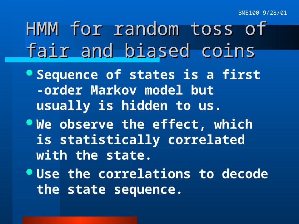
HMM for random toss of fair and HMM for random toss of fair and biased coinsbiased coinsSequence of states is a first -order
Markov model but usually is hidden to us.
We observe the effect, which is statistically correlated with the state.
Use the correlations to decode the state sequence.

BME100 9/28/01
HMM for fair and biased coinsHMM for fair and biased coins
Sequence of states: q = FFFFBBBFFFFF
Observed sequence: x = HTTHTTTTHHTH
With complete information, can compute:
P(x,q) = 0.5 * 0.5 * 0.8 * 0.5 * 0.8 * 0.5 * 0.8 * 0.5 * 0.2 * 0.9 . . .
q
)q,x(P)x(POtherwise:
BME100 9/28/01
Three key HMM algorithmsThree key HMM algorithms
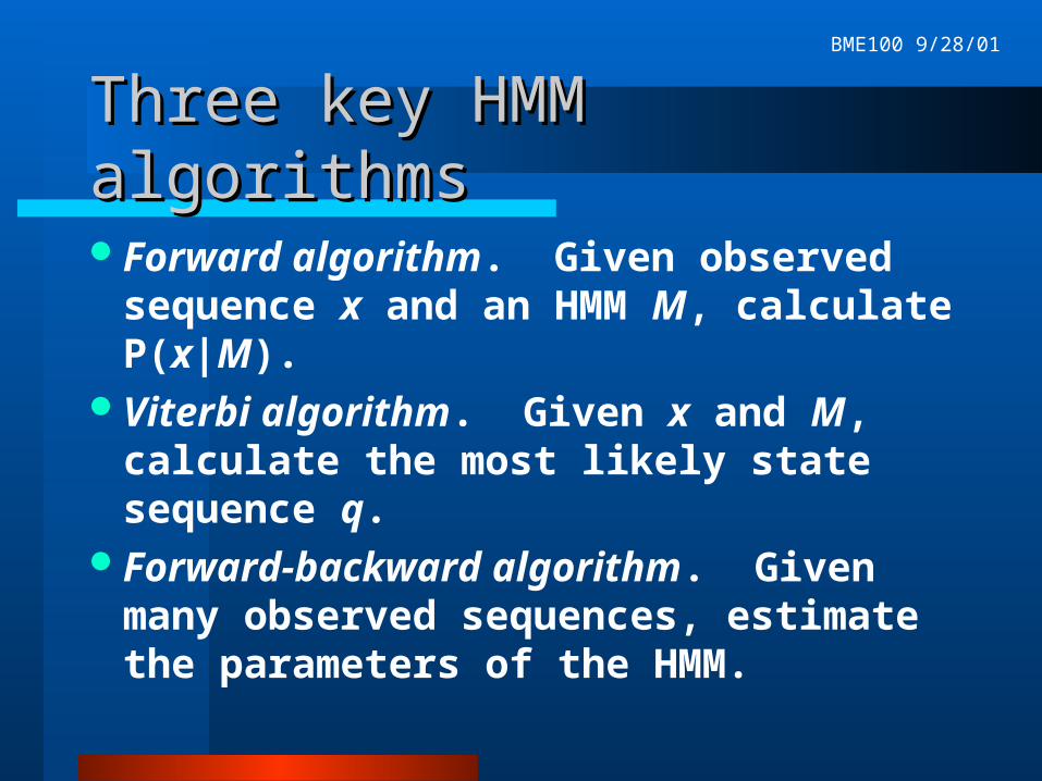
Forward algorithm. Given observed sequence x and an HMM M, calculate P(x|M).
Viterbi algorithm. Given x and M, calculate the most likely state sequence q.
Forward-backward algorithm. Given many observed sequences, estimate the parameters of the HMM.

BME100 9/28/01
Some HMM TopologiesSome HMM Topologies

BME100 9/28/01
Modeling protein families with Modeling protein families with linear profile HMMslinear profile HMMsObserved sequence is the amino acid
sequence of a protein.Typically want to model a group of
related proteins.Model states and transitions will be
based on a multiple alignment of the group.
No transitions from right to left.
BME100 9/28/01
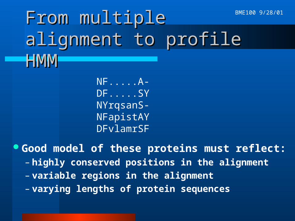
From multiple alignment to From multiple alignment to profile HMMprofile HMM
Good model of these proteins must reflect:– highly conserved positions in the alignment– variable regions in the alignment– varying lengths of protein sequences
NF.....A-DF.....SYNYrqsanS-NFapistAYDFvlamrSF
BME100 9/28/01
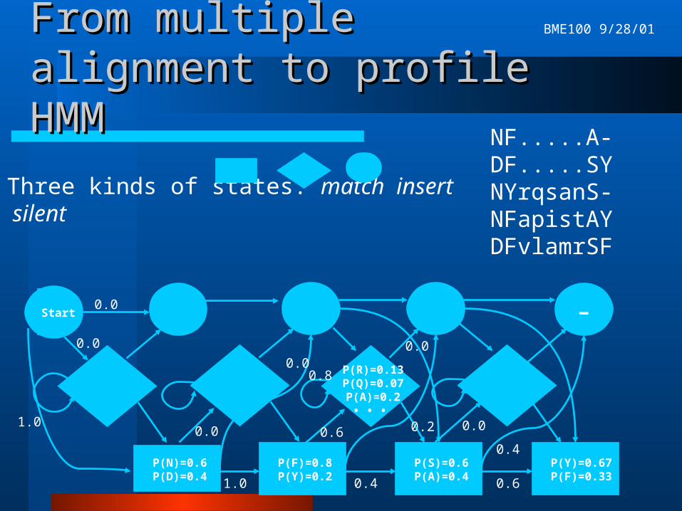
From multiple alignment to From multiple alignment to profile HMMprofile HMM
NF.....A-DF.....SYNYrqsanS-NFapistAYDFvlamrSF
P(N)=0.6P(D)=0.4
P(R)=0.13P(Q)=0.07P(A)=0.2
• • •
Three kinds of states: match insert silent
P(F)=0.8P(Y)=0.2
1.0
0.8
0.6
P(S)=0.6P(A)=0.4
P(Y)=0.67P(F)=0.33
0.4
-
0.2
0.4
0.6
0.0
0.00.0
0.0
Start
0.0
0.0
1.0
BME100 9/28/01
Finding probability of a sequence Finding probability of a sequence with an HMMwith an HMMOnce we have an HMM for a group of
proteins, we are often interested in how well a new sequence fits the model.
We want to compute a probability for our sequence with respect to the model.
BME100 9/28/01
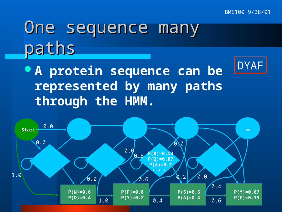
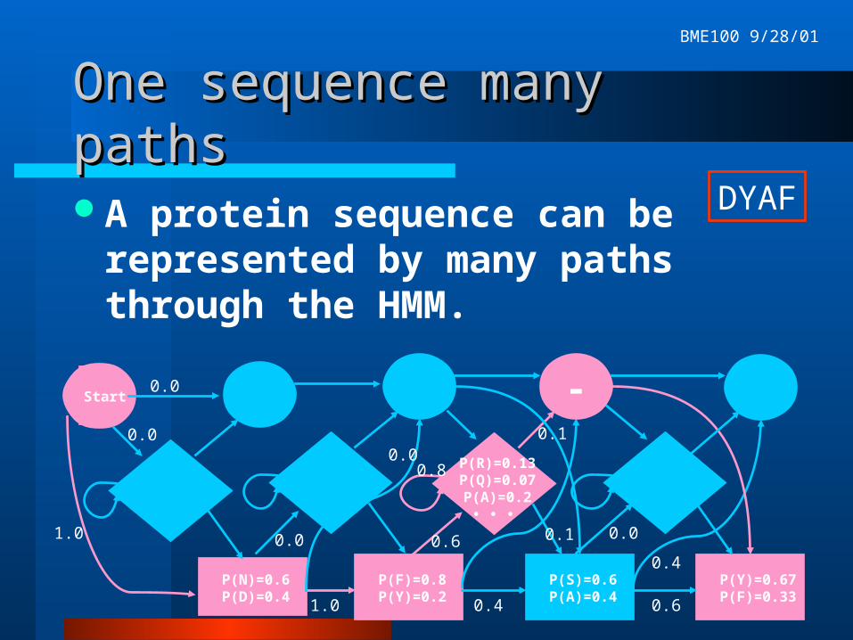
One sequence many pathsOne sequence many paths
A protein sequence can be represented by many paths through the HMM.
P(N)=0.6P(D)=0.4
-
P(F)=0.8P(Y)=0.2
P(S)=0.6P(A)=0.4
P(Y)=0.67P(F)=0.33
P(R)=0.13P(Q)=0.07P(A)=0.2
• • •
1.0 0.4
0.6
0.6
0.8
0.2
0.40.0
0.00.0
0.0
DYAF
Start
0.0
0.0
1.0
BME100 9/28/01
One sequence many pathsOne sequence many paths
A protein sequence can be represented by many paths through the HMM.
P(N)=0.6P(D)=0.4
P(F)=0.8P(Y)=0.2
P(S)=0.6P(A)=0.4
P(Y)=0.67P(F)=0.33
P(R)=0.13P(Q)=0.07P(A)=0.2
• • •
1.0 0.4
0.6
0.6
0.8
0.1
0.4
-
0.0
0.00.1
0.0
DYAF
Start
0.0
0.0
1.0
BME100 9/28/01
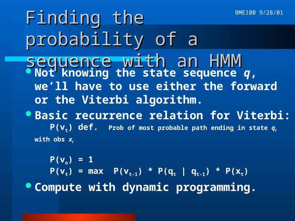
Finding the probability of a Finding the probability of a sequence with an HMMsequence with an HMMNot knowing the state sequence q, we’ll
have to use either the forward or the Viterbi algorithm.
Basic recurrence relation for Viterbi: P(vt) def. Prob of most probable path ending in state qt with obs xt P(vo) = 1 P(vt) = max P(vt-1) * P(qt | qt-1) * P(xt)
Compute with dynamic programming.
BME100 9/28/01
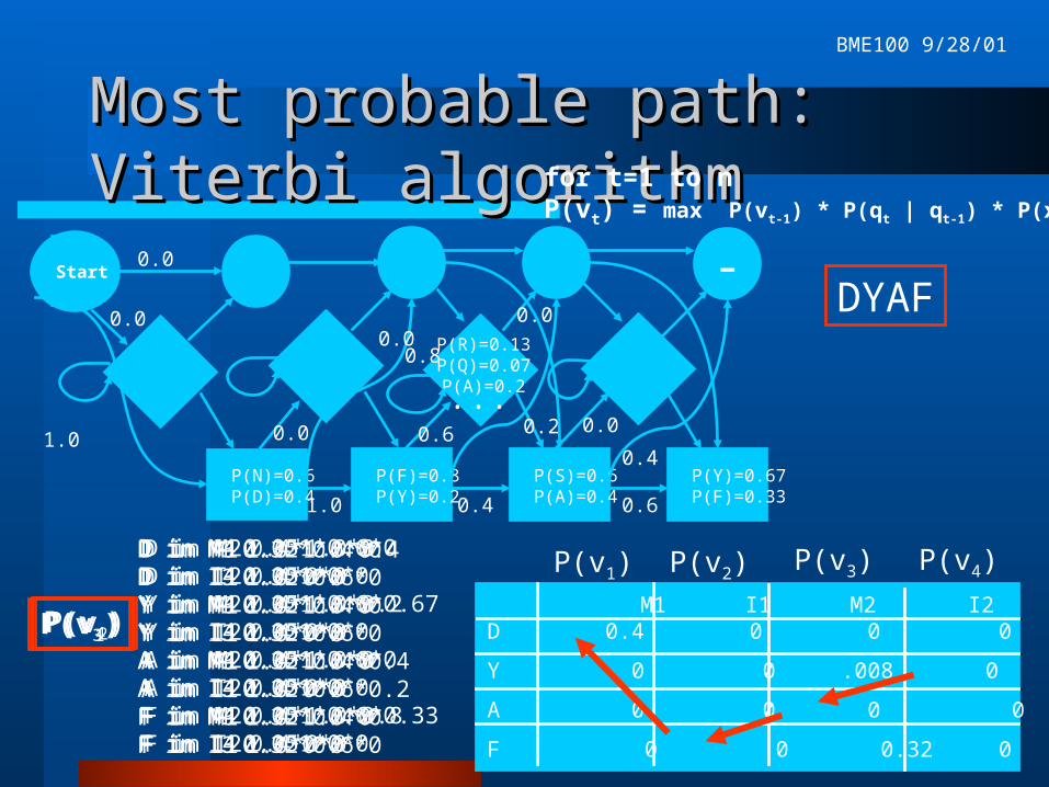
M1 I1 M2 I2 M3 I3 M4 I4D 0.4 0 0 0 0 0 0 0
Y 0 0 .008 0 0 0 .021 0
A 0 0 0 0 .051 .038 0 0
F 0 0 0.32 0 0 0 .01 0
Most probable path: Viterbi Most probable path: Viterbi algorithmalgorithm
P(N)=0.6P(D)=0.4
-
P(F)=0.8P(Y)=0.2
P(S)=0.6P(A)=0.4
P(Y)=0.67P(F)=0.33
P(R)=0.13P(Q)=0.07P(A)=0.2
• • •
1.0 0.4
0.6
0.6
0.8
0.2
0.40.0
0.00.0
0.0
DYAFStart
0.0
0.0
1.0
for t=1 to nP(vt) = max P(vt-1) * P(qt | qt-1) * P(xt)
D in M1 1.0*1.0*0.4D in I1 1.0*0*0Y in M1 1.0*1.0*0Y in I1 1.0*0*0A in M1 1.0*1.0*0A in I1 1.0*0*0F in M1 1.0*1.0*0F in I1 1.0*0*0
P(v1)
P(v1) P(v2) P(v3) P(v4)D in M2 0.4*1.0*0D in I2 0.4*0*0Y in M2 0.4*1.0*0.2Y in I2 0.4*0*0A in M2 0.4*1.0*0A in I2 0.4*0*0F in M2 0.4*1.0*0.8F in I2 0.4*0*0
P(v2)
D in M3 0.32*0.4*0D in I3 0.32*0.6*0Y in M3 0.32*0.4*0Y in I3 0.32*0.6*0A in M3 0.32*0.4*0.4A in I3 0.32*0.6*0.2F in M3 0.32*0.4*0F in I3 0.32*0.6*0
P(v3)
D in M4 0.051*0.6*0D in I4 0.051*0*0Y in M4 0.051*0.6*0.67Y in I4 0.051*0*0A in M4 0.051*0.6*0A in I4 0.051*0*0F in M4 0.051*0.6*0.33F in I4 0.051*0*0
P(v4)
BME100 9/28/01
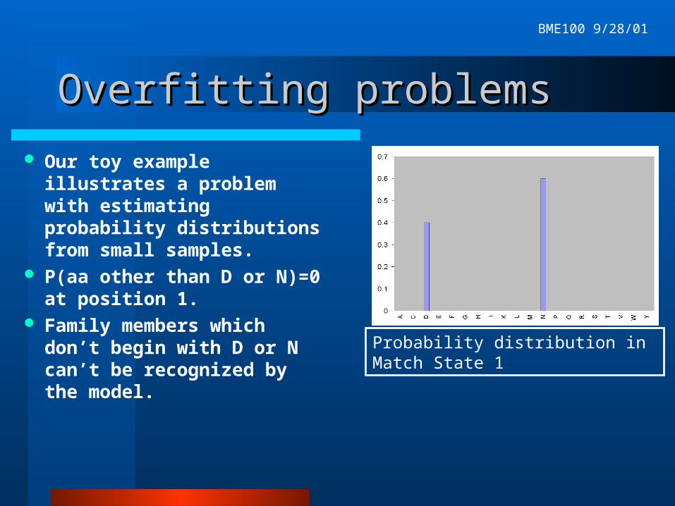
Overfitting problemsOverfitting problems
Our toy example illustrates a problem with estimating probability distributions from small samples.
P(aa other than D or N)=0at position 1.
Family members which don’t begin with D or N can’t be recognized by the model.
Probability distribution in Match State 1
BME100 9/28/01
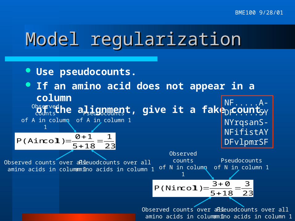
Model regularizationModel regularization
Use pseudocounts. If an amino acid does not appear in a column
of the alignment, give it a fake count. NF.....A-DF.....SYNYrqsanS-NFifistAYDFvlpmrSF23
1
185
10 1) colin P(A
Observed countsof A in column 1
Pseudocountsof A in column 1
Observed counts over all amino acids in column 1
Pseuodcounts over allamino acids in column 1
23
3
185
03 1) colin P(N
Observed countsof N in column 1
Pseudocountsof N in column 1
Observed counts over all amino acids in column 1
Pseuodcounts over allamino acids in column 1
BME100 9/28/01
Model regularizationModel regularization
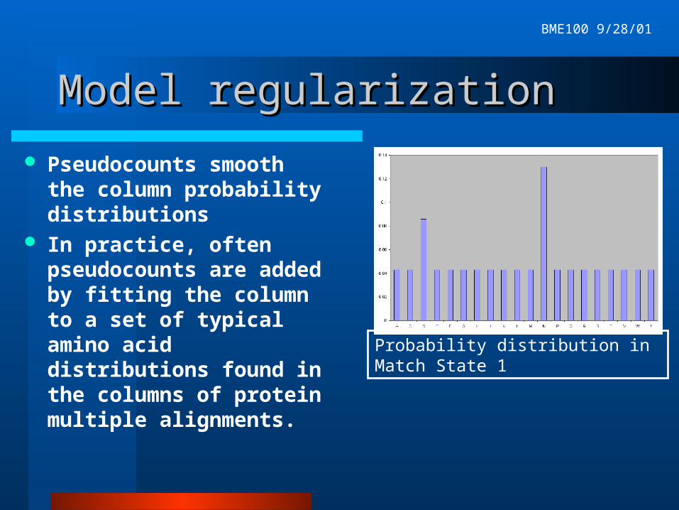
Pseudocounts smooth the column probability distributions
In practice, often pseudocounts are added by fitting the column to a set of typical amino acid distributions found in the columns of protein multiple alignments.
Probability distribution in Match State 1

BME100 9/28/01
To come:To come:
HMMs can be used to automatically produce a high-quality multiple alignment.
Active areas of research:– Building HMMs that can recognize very
distantly related proteins–Multi-track HMMs
Top Related