


Languages
Pages
Legal

Hedge Fund Leverage∗
Andrew Ang†
Columbia University and NBER
Sergiy Gorovyy‡
Columbia University
Gregory B. van Inwegen§
Citi Private Bank
This Version: 25 January, 2011
JEL Classification: G11, G18, G23, G32Keywords: Capital structure, long-short positions,
alternative investments, exposure, hedging, systemic risk
∗We thank Viral Acharya, Tobias Adrian, Zhiguo He, Arvind Krishnamurthy, Suresh Sundaresan,Tano Santos, an anonymous referee, and seminar participants at Columbia University and Risk USA2010 for helpful comments.
†Email: [email protected]; WWW: http://www.columbia.edu/∼aa610.‡Email: [email protected]§Email: [email protected]
Hedge Fund Leverage
Abstract
We investigate the leverage of hedge funds in the time series and cross section. Hedge fund
leverage is counter-cyclical to the leverage of listed financial intermediaries and decreases prior
to the start of the financial crisis in mid-2007. Hedge fund leverage is lowest in early 2009 when
the market leverage of investment banks is highest. Changes in hedge fund leverage tend to be
more predictable by economy-wide factors than by fund-specific characteristics. In particular,
decreases in funding costs and increases in market values both forecast increases in hedge fund
leverage. Decreases in fund return volatilities predict future increases in leverage.

1 Introduction
The events of the financial crisis over 2007-2009 have made clear the importance of leverage of
financial intermediaries to both asset prices and the overall economy. The observed “delever-
aging” of many listed financial institutions during this period has been the focus of many regu-
lators and the subject of much research.1 The role of hedge funds has played a prominent role
in these debates for several reasons. First, although in the recent financial turbulence no single
hedge fund has caused a crisis, the issue of systemic risks inherent in hedge funds has been
lurking since the failure of the hedge fund LTCM in 1998.2 Second, within the asset manage-
ment industry, the hedge fund sector makes the most use of leverage. In fact, the relatively high
and sophisticated use of leverage is a defining characteristic of the hedge fund industry. Third,
hedge funds are large counterparties to the institutions directly overseen by regulatory authori-
ties, especially commercial banks, investment banks, and other financial institutions which have
received large infusions of capital from governments.
However, while we observe the leverage of listed financial intermediaries through periodic
accounting statements and reports to regulatory authorities, little is known about hedge fund
leverage despite the proposed regulations of hedge funds in the U.S. and Europe. This is be-
cause hedge funds are by their nature secretive, opaque, and have little regulatory oversight.
Leverage plays a central role in hedge fund management. Many hedge funds rely on leverage
to enhance returns on assets which on an unlevered basis would not be sufficiently high to at-
tract funding. Leverage amplifies or dampens market risk and allows funds to obtain notional
exposure at levels greater than their capital base. Leverage is often employed by hedge funds
to target a level of return volatility desired by investors. Hedge funds use leverage to take ad-
vantage of mispricing opportunities by simultaneously buying assets which are perceived to
be underpriced and shorting assets which are perceived to be overpriced. Hedge funds also
dynamically manipulate leverage to respond to changing investment opportunity sets.
We are the first paper, to our knowledge, to formally investigate hedge fund leverage using
1 See, for example, Adrian and Shin (2009), Brunnermeier (2009), Brunnermeier and Pedersen (2009), and He,
Khang, and Krishnamurthy (2010), among many others.2 Systemic risks of hedge funds are discussed by the President’s Working Group on Financial Markets (1999),
Chan et al. (2007), Kambhu, Schuermann, and Stiroh (2007), Financial Stability Forum (2007), and Banque de
France (2007).
1

actual leverage ratios with a unique dataset from a fund-of-hedge funds. We track hedge fund
leverage in time series from December 2004 to October 2009, a period which includes the
worst periods of the financial crisis from 2008 to early 2009. We characterize the cross section
of leverage: we examine the dispersion of leverage across funds and investigate the macro and
fund-specific determinants of future leverage changes. We compare the leverage and exposure
of hedge funds with the leverage and total assets of listed financial companies. As well as
characterizing leverage at the aggregate level, we investigate the leverage of hedge fund sectors.
The prior work on hedge fund leverage are only estimates (see, e.g., Banque de France,
2007; Lo, 2008) or rely only on static leverage ratios reported by hedge funds to the main
databases. For example, leverage at a point in time is used by Schneeweis et al. (2004) to inves-
tigate the relation between hedge fund leverage and returns. Indirect estimates of hedge fund
leverage are computed by McGuire and Tsatsaronis (2008) using factor regressions with time-
varying betas. Even without considering the sampling error in computing time-varying factor
loadings, this approach requires that the complete set of factors be correctly specified, otherwise
the implied leverage estimates suffer from omitted variable bias. Regressions may also not ade-
quately capture abrupt changes in leverage. Other work by Brunnermeier and Pedersen (2009),
Gorton and Metrick (2009), Adrian and Shin (2010), and others, cite margin requirements, or
haircuts, as supporting evidence of time-varying leverage taken by proprietary trading desks at
investment banks and hedge funds. These margin requirements give maximum implied lever-
age, not the actual leverage that traders are using. In contrast, we analyze actual leverage ratios
of hedge funds.
Our work is related to several large literatures, some of which have risen to new prominence
with the financial crisis. First, our work is related to optimal leverage management by hedge
funds. Duffie, Wang and Wang (2008) and Dai and Sundaresan (2010) derive theoretical models
of optimal leverage in the presence of management fees, insolvency losses, and funding costs
and restrictions at the fund level. At the finance sector level, Acharya and Viswanathan (2008)
study optimal leverage in the presence of moral hazard and liquidity effects showing that due
to deleveraging, bad shocks that happen in good times are more severe. A number of au-
thors have built equilibrium models where leverage affects the entire economy. In Fostel and
Geanakoplos (1998), economy-wide equilibrium leverage rises in times of low volatility and
2

falls in periods where uncertainty is high and agents have very disperse beliefs. Leverage am-
plifies liquidity losses and leads to over-valued assets during normal times. Stein (2009) shows
that leverage may be chosen optimally by individual hedge funds, but this may create a fire-
sale externality causing systemic risk by hedge funds simultaneously unwinding positions and
reducing leverage. There are also many models where the funding available to financial in-
termediaries, and hence leverage, affects asset prices. In many of these models, deleveraging
cycles are a key part of the propagating mechanism of shocks.3 Finally, a large literature in cor-
porate finance examines how companies determine optimal leverage. Recently, Welch (2004)
studies the determinants of firm debt ratios and finds that approximately two-thirds of variation
in corporate leverage ratios is due to net issuing activity.
The remainder of the paper is organized as follows. We begin in Section 2 by defining and
describing several features of hedge fund leverage. Section 3 describes our data. Section 4 out-
lines the estimation methodology which allows us to take account of missing values. Section 5
presents the empirical results. Finally, Section 6 concludes.
2 The Mechanics of Hedge Fund Leverage
2.1 Gross, Net, and Long-Only Leverage
A hedge fund holds risky assets in long and short positions together with cash. Leverage mea-
sures the extent of the relative size of the long and short positions in risky assets relative to the
size of the portfolio. Cash can be held in both a long position or a short position, where the
former represents short-term lending and the latter represents short-term borrowing. The assets
under management (AUM) of the fund is cash plus the difference between the fund’s long and
short positions and is the value of the claim all investors have on the fund. The net asset value
per share (NAV) is the value of the fund per share and is equal to AUM divided by the number
of shares. We use the following three definitions of leverage, which are also widely used in
industry:
3 See, for example, Gromb and Vayanos (2002), He and Krishnamurthy (2009), Brunnermeier and Pedersen
(2009), and Adrian and Shin (2010).
3
Gross Leverage is the sum of long and short exposure per share divided by NAV. This defi-
nition implicitly treats both the long and short positions as separate sources of profits in their
own right, as would be the case for many long-short equity funds. This leverage measure over-
states risk if the short position is used for hedging and does not constitute a separate active bet.
If the risk of the short position by itself is small, or the short position is usually taken together
with a long position, a more appropriate definition of leverage may be:
Net Leverage is the difference between long and short exposure per share expressed as a pro-
portion of NAV. The net leverage measure captures only the long positions representing active
positions which are not perfectly offset by short hedges, assuming the short positions represent
little risk by themselves. Finally, we consider,
Long-Only Leverage or Long Leverage is defined as the long positions per share divided by
NAV. Naturally, by ignoring the short positions, long-only leverage could result in a large
under-estimate of leverage, but we examine this conservative measure because the reporting
requirements of hedge fund positions by the SEC involve only long positions.4 We also investi-
gate if long leverage behaves differently from gross or net leverage, or put another way, if hedge
funds actively manage their long and short leverage positions differently.
Only a fund 100% invested in cash has a leverage of zero for all three leverage definitions.
Furthermore, for a fund employing only levered long positions, all three leverage measure coin-
cide. Thus, active short positions induce differences between gross, net, and long-only leverage.
Appendix A illustrates these definitions of leverage for various hedge fund portfolios.
2.2 How do Hedge Funds Obtain Leverage?
Hedge funds obtain leverage through a variety of means, which depend on the type of securities
traded by the hedge fund, the creditworthiness of the fund, and the exchange, if any, on which
4 Regulation 13-F filings are required by any institutional investor managing more than $100 million. Using
these filings, Brunnermeier and Nagel (2004) examine long-only hedge fund positions in technology stocks during
the late 1990s bull market.
4

the securities are traded. Often leverage is provided by a hedge fund’s prime broker, but not
all hedge funds use prime brokers.5 By far the vast majority of leverage is obtained through
short-term funding as there are very few hedge funds able to directly issue long-term debt or
secure long-term borrowing.
In the U.S., regulations govern the maximum leverage permitted in many exchange-traded
markets. The Federal Reserve Board’s Regulation T (Reg T) allows investors to borrow up to
a maximum 50% of a position on margin (which leads to a maximum level of exposure equal
1/0.5 = 2). For a short position, Reg T requires that short sale accounts hold collateral of
50% of the value of the short implying a maximum short exposure of two. By establishing
offshore investment vehicles, hedge funds can obtain “enhanced leverage” higher than levels of
than allowable by Reg T. Prime brokers have established facilities overseas in less restrictive
jurisdictions in order to provide this service. Another way to obtain higher leverage than allowed
by Reg T is “portfolio margining” which is another service provided by prime brokers. Portfolio
margining was approved by the SEC in 2005 and allows margins to be calculated on a portfolio
basis, rather than on a security by security basis.6
Table 1 reports typical margin requirements (“haircuts”) required by prime brokers or other
counterparties. The last column of the Table 1 lists the typical levels of leverage able to be ob-
tained in each security market, that are the inverse of the margin requirements. This data is ob-
tained at March 2010 by collating information from prime brokers and derivatives exchanges.7
Note that some financial instruments, such as derivatives and options, have embedded leverage
in addition to the leverage available from external financing. The highest leverage is available
in Treasury, foreign exchange, and derivatives security markets such as interest rate and foreign
exchange swaps. These swap transactions are over the counter and permit much higher levels
of leverage than Reg T. These securities enable investors to have large notional exposure with
little or no initial investment or collateral. Similarly, implied leverage is high in futures markets
5 In addition to providing financing for leverage, prime brokers provide hedge fund clients with risk management
services, execution, custody, daily account statements, and short sale inventory for stock borrowing. In some cases,
prime brokers provide office space, computing and trading infrastructure, and may even contribute capital.6 Portfolio margining only applies to “hardwired” relations, such as calls and puts on a stock, and the underlying
stock itself, rather than to any statistical correlations between different assets.7 Brunnermeier and Pedersen (2009) and Gorton and Metrick (2009) show that margin requirements changed
substantially over the financial crisis.
5
because the margin requirements there are much lower than in the equity markets.
Based on the dissimilar margin requirements of different securities reported in Table 1, it is
not surprising that hedge fund leverage is heterogeneous and depends on the type of investment
strategy employed by the fund. Our results below show that funds engaged in relative value
strategies, which trade primarily fixed income, swaps, and other derivatives, have the highest
average gross leverage of 4.8 through the sample. Some relative value funds in our sample
have gross leverage greater than 30. Credit funds which primarily hold investment grade and
high yield corporate bonds and credit derivatives have an average gross leverage of 2.4 in our
sample. Hedge funds in the equity and event driven strategies mainly invest in equity and
distressed corporate debt and hence have lower leverage. In particular, equity and event driven
funds have average gross leverage of 1.6 and 1.3, respectively over our sample.
The cost of leverage to hedge funds depends on the method used to obtain leverage. Prime
brokers typically charge a spread over LIBOR to hedge fund clients who are borrowing to fund
their long positions and brokers pay a spread below LIBOR for cash deposited by clients as
collateral for short positions. These spreads are higher for less credit worthy funds and are
also higher when securities being financed have high credit risk or are more volatile. The cost
of leverage through prime brokers reflects the costs of margin in traded derivatives markets.
We include instruments capturing funding costs like LIBOR and interest rate spreads in our
analysis.
In many cases, there are maximum leverage constraints imposed by the providers of lever-
age on hedge funds. Hedge fund managers make a decision on optimal leverage as a function
of the type of the investment strategy, the perceived risk-return trade-off of the underling trades,
and the cost of obtaining leverage, all subject to exogenously imposed leverage limits. Financ-
ing risk is another consideration as funding provided by prime brokers can be subject to sudden
change. In contrast, leverage obtained through derivatives generally have lower exposure to
funding risk. Prime brokers have the ability to pull financing in many circumstances, for exam-
ple, when performance or NAV triggers are breached. Dai and Sundaresan (2010) show that this
structure effectively leaves the hedge funds short an option vis-a-vis their prime broker. Adding
further risk to this arrangement is the fact that the hedge fund is also short an option vis-a-vis
another significant financing source, their client base, which also has the ability to pull financ-
6
ing following terms stipulated by the offering memorandum.8 We do not consider the implicit
leverage in these funding options in our analysis as we are unable to obtain data on hedge fund
prime broker agreements or the full set of investment memoranda of hedge fund clients; our
analysis applies only to the leverage reported by hedge funds in their active strategies.9
2.3 Reported Hedge Fund Leverage
An important issue with hedge fund leverage is which securities are included in the firm-wide
leverage calculation and how the contribution of each security to portfolio leverage is calculated.
The most primitive form of leverage calculation is unadjusted balance sheet leverage, which is
simply the value of investment assets, not including notional exposure in derivatives, divided
by equity capital. Since derivatives exposure for hedge funds can be large, this understates, in
many cases dramatically, economic risk exposure.
To remedy this shortcoming, leverage is often adjusted for derivative exposure by taking
delta-adjusted notional values of derivative contracts.10 For example, in order to account for
the different volatility and beta exposures of underlying investments, hedge funds often beta-
adjust the exposures of (cash) equities by upward adjusting leverage for high-beta stock hold-
ings. Likewise, (cash) bond exposures are often adjusted to account for the different exposures
to interest rate factors. In particular, the contribution of bond investments to the leverage cal-
culation is often scaled up or down by calculating a 10-year equivalent bond position. Thus, an
investment of $100 in a bond with twice the duration of a 10-year bond would have a position
of $200 in the leverage calculation. The issues of accounting for leverage for swaps and futures
affect fixed income hedge funds the most and long-short equity hedge funds the least. For this
reason we break down leverage statistics by hedge fund sectors.
8 In many cases, hedge funds have the ability to restrict outflows by invoking gates even after lockup periods
have expired (see, for example, Ang and Bollen, 2010).9 Dudley and Nimalendran (2009) estimate funding costs and funding risks for hedge funds, which are not
directly observable, using historical data on margins from futures exchanges and VIX volatility. They do not
consider hedge fund leverage.10 Many hedge funds account for the embedded leverage in derivatives positions through internal reporting
systems or external, third-party risk management systems like Riskmetrics. These risk system providers compute
risk statistics like deltas, left-hand tail measures of risk like Value-at-Risk, and implied leverage at both the security
level and the aggregate portfolio level. Riskmetrics allows hedge funds to “pass through” their risk statistics to
investors who can aggregate positions across several funds.
7

Funds investing primarily in futures, especially commodities, report a margin-to-equity ra-
tio, which is the amount of cash used to fund margin divided by the nominal trading level of
the fund. This measure is proportional to the percentage of available capital dedicated to fund-
ing margin requirements. It is frequently used by commodity trading advisors as a gauge of
their market exposure. Other funds investing heavily in other zero-cost derivative positions like
swaps also employ similar measures based on ratios of nominal, or adjusted nominal exposure,
to collateral cash values to compute leverage.
Thus, an important caveat with our analysis is that leverage is not measured in a consistent
fashion across hedge funds and the hedge funds in our sample use different definitions of lever-
age. Our data is also self-reported by hedge funds. These effects are partially captured in our
analysis through fund fixed effects. Our analysis focuses on the common behavior of leverage
across hedge funds rather than explaining the movements in leverage of a specific hedge fund.
3 Data
3.1 Macro Data
We capture the predictable components of hedge fund leverage by various aggregate market
price variables, which we summarize in Appendix B. We graph two of these variables in Fig-
ure 1. We plot the average cost of protection from a default of major “investment banks” (Bear
Stearns, Citibank, Credit Suisse, Goldman Sachs, HSBC, JP Morgan, Lehman Brothers, Merrill
Lynch, and Morgan Stanley) computed using credit default swap (CDS) contracts in the solid
line with the scale on the left-hand axis. This is the market-weighted cost of protection per year
against default of each firm. Our selected firms are representative of broker/dealers and invest-
ment banking activity and we refer to them as investment banks even though many of them are
commercial banks and some became commercial banks during the sample period.
In Figure 1 we also plot the VIX volatility index in the dotted line with the scale on the right-
hand axis. The correlation between VIX and investment bank CDS protection is 0.89. Both of
these series are low at the beginning of the sample and then start to increase in mid-2007,
which coincides with the initial losses in subprime mortgages and other certain securitized
markets. In late 2008, CDS spreads and VIX increase dramatically after the bankruptcy of
8

Lehman Brothers, with VIX reaching a peak of 60% at the end of October 2008 and the CDS
spread reaching 3.55% per annum in September 2008. In 2009, both CDS and VIX decline
after the global financial sector is stabilized.
Our other macro series are monthly returns on investment banks, monthly returns on the
S&P 500, the three-month LIBOR rate, and the three-month Treasury over Eurodollar (TED)
spread. The LIBOR and TED spreads are good proxies for the aggregate cost of short-term
borrowing for large financial institutions. Prime brokers pass on at least the LIBOR and TED
spread costs to their hedge fund clients plus a spread. Finally, we also include the term spread,
which is the difference between the 10-year Treasury bond yield and the yield on three-month
T-bills. This captures the slope of the yield curve, which under the Expectations Hypothesis is
a forward-looking measure of future short-term interest rates and thus provides a simple way of
estimating future short-term borrowing costs.
3.2 Hedge Fund Data
Our hedge fund data is obtained from a large fund-of-hedge-funds (which we refer to as the
“Fund”). The original dataset from the Fund contains over 45,000 observations of 758 funds
from February 1977 to December 2009. In addition to hedge fund leverage, our data includes
information on the strategy employed by the hedge funds, monthly returns, NAVs, and AUMs.
The hedge funds are broadly representative of the industry and contain funds managed in a
variety of different styles including global macro funds, fundamental stock-picking funds, credit
funds, quantitative funds, and funds investing using technical indicators. The hedge funds invest
both in specific asset classes, for example, fixed income or equities, and also across global asset
classes. Our data includes both U.S. and international hedge funds, but all returns, NAVs, and
AUMs are in US dollars.
An important issue is whether the hedge funds in the database exhibit a selection bias.
In particular, do the hedge funds selected by the Fund have better performance and leverage
management than a typical hedge fund? The Fund selects managers using both a “top down” and
a “bottom up” approach. The former involves selecting funds in various sector allocation bands
for the Fund’s different fund-of-fund portfolios. The latter involves searching for funds, or
re-allocating money across existing funds, using a primarily qualitative, proprietary approach.
9

Leverage is a consideration in choosing funds, but it is only one of many factors among the
usual suspects – Sharpe ratios and other performance criteria, due diligence considerations,
network, manager quality, transparency, gates and restrictions, sector composition, investment
style, etc. The Fund did not add leverage to its products and only very rarely asked hedge
funds to provide a customized volatility target or to provide leverage which differed from the
hedge funds’ existing product offerings. There is no reason to believe that the Fund’s selection
procedure results in funds with leverage management practices that are significantly different
to the typical hedge fund.
Our Fund database includes funds that are present in TASS, CISDM, Barclay Hedge, or
other databases commonly used in research and also includes other funds which do not report
to the public hedge fund databases. This mitigates the reporting bias of the TASS database (see
Malkiel and Saha, 2005; Ang, Rhodes-Kropf, and Zhao, 2008; Agarwal, Fos, and Jiang, 2010).
However, the composition by sector is similar to the overall sector weighting of the industry as
reported by TASS and Barclay Hedge. Survival biases are mitigated by the fact that often hedge
funds enter the database not when they receive funds from the Fund, but several months prior to
the Fund’s investment and they often exit the database several months after disinvestment. Our
database also includes hedge funds which terminate due to poor performance. The aggregate
performance of the Fund is similar to the performance of the main hedge fund indexes.
3.2.1 Hedge Fund Leverage
Leverage is reported by different hedge funds at various frequencies and formats, which are
standardized by the Fund. Appendix C discusses some of these formats. Most reporting is
at the monthly frequency, but some leverage numbers are reported quarterly or even less fre-
quently. For those funds reporting leverage at the quarterly or at lower frequencies, the Fund
is often able to obtain leverage numbers directly from the hedge fund managers at other dates
through a combination of analyst site visits and calls to hedge fund managers. The data is of
high quality because the funds undergo thorough due diligence by the Fund. In addition, the
performance and risk reports are audited, and the Fund conducts regular, intensive monitoring
of the investments made in the individual hedge funds.
10

3.2.2 Hedge Fund Returns, Volatilities, and Flows
We have monthly returns on all the hedge funds. These returns are actual realized returns, rather
than returns reported to the publicly available databases. In addition to examining the relation
between past returns and leverage, we construct volatilities from the returns. We construct
monthly hedge fund volatility using the sample standard deviation of returns over the past 12
months. Figure 2 plots the volatilities of all hedge funds and different hedge fund strategies
over the sample. The volatilities follow the same broad trend and are approximately the same.
This is consistent with hedge funds using leverage to scale returns to similar volatility levels.
Figure 2 shows that at the beginning of the sample, hedge fund volatilities were around 3%
per month and reach a low of around 2% per month in 2006. As subprime mortgages start to
deteriorate in mid-2007, hedge fund return volatility starts to increase and reaches 4-5% per
month by 2009. Volatility stays at this high level until the end of the sample in October 2009.
This is because we use rolling 12-month sample volatilities which include the very volatile,
worst periods of the financial crisis 12 months prior to October 2009.
Figure 3 compares the rolling 12-month volatilities of hedge fund returns in the data sample
with the rolling 12-month volatilities of hedge fund returns in the HFR database for the Decem-
ber 2004 - October 2009 time period. We observe that the average volatilities of hedge funds
in the data closely track the median hedge fund volatility in the HFR database. Thus, the Funds
hedge funds have very similar return behavior as the typical hedge fund reported on the publicly
available databases. Since hedge funds often use leverage to target particular levels of volatility,
this partially alleviates concerns that the Fund’s hedge funds have atypical leverage policies.
In addition to hedge fund volatility, we also use hedge fund flows as a control variable.
We construct hedge fund-level flows over the past three months using the return and AUM
information from the following formula:
Flowt =AUMt
AUMt−3
− (1 +Rt−2)(1 +Rt−1)(1 +Rt) (1)
where Flowt is the past three-month flow in the hedge fund, AUMt is assets under management
at time t and Rt is the hedge fund return from t − 1 to t. The flow formula in equation (1)
is used by Chevalier and Ellison (1997), Sirri and Tufano (1998), and Agarwal, Daniel, and
Naik (2009), among others. We compute three-month flows as the flows over the past month
11

tend to be very volatile. We also compute past three-month hedge fund flows for the aggregate
hedge fund industry as measured by the Barclay Hedge database using equation (1).
3.3 Summary Statistics
We clean the raw data from the Fund and impose two filters. First, often investments are made
by the Fund in several classes of shares of a given hedge fund. All of these share classes have
almost identical returns and leverage ratios. We use the share class with the longest history or
the share class representing the largest AUM. Our second filter is that we require funds to have
at least two years of leverage observations. The final sample spans December 2004 to October
2009 and thus our sample includes the poor returns of quantitative funds during Summer 2007
(see Khandani and Lo, 2007) and the financial crisis of 2008 and early 2009. There are at least
63 funds in our sample at any one time. The maximum number of funds at any given month is
163 over the sample period.
Panel A of Table 2 lists the number of observations and number of hedge funds broken
down by strategy. The strategies are defined by the Fund and do not exactly correspond to the
sector definitions employed by TASS, Barclay Hedge, CSDIM or other hedge fund databases
(which themselves employ arbitrary sector definitions). The TASS categories of fixed income
arbitrage and convertible arbitrage fall under the Fund’s relative value sector. In the relative
value sector, hedge funds invest in both developed and emerging markets and can also invest
in a variety of different asset classes. Most of the Fund’s investments have been in long-short
equity funds in the equity category and this is also by far the largest hedge fund sector in TASS,
as reported, for example, by Chan et al. (2007). At the last month of our sample, October 2009,
the proportion of equity funds reported in Barclay Hedge, not including multi-strategy, other,
and sector-specific categories, is also over 40%.
After our data filters, there are a total of 208 unique hedge funds in our sample with 8,136
monthly observations. Over half (114) of the funds in our sample run long-short equity strate-
gies. The number of funds in the areas of credit and relative value are 21 and 36, respectively.
The remaining 37 funds are in the event driven strategy, which are mainly merger arbitrage and
distressed debt. The number of funds reported in Panel A of Table 2 is large enough for reliable
12
inference when averaged across strategies and across all hedge funds.11
In Panel B of Table 2, we report summary statistics of all the hedge fund variables observed
in the sample. These statistics should be carefully interpreted because they do not sample all
hedge funds at the same frequency and there are missing observations in the raw data. Panel B
reports that the average gross leverage across all hedge funds is 2.13 with a volatility of 0.62.
This volatility is computed using only observed data and the true volatility of leverage, after
estimating the unobserved values, will be lower, as we show below. Nevertheless, it is clear
that hedge fund leverage changes over time. Even without taking into account missing observa-
tions, this volatility is much lower than the volatility of leverage reported in the estimations of
McGuire and Tsataronis (2008) using factor regressions. This discrepancy could possibly result
from the large error in their procedure of inferring leverage from estimated factor coefficients
in regressions on short samples. Individual gross hedge fund leverage is also persistent, with
an average autocorrelation of 0.68 across all the hedge funds. Again because of unobserved
leverage ratios, this persistence is biased downwards and we report more accurate measures of
autocorrelation taking into account other predictive variables below.
Panel B of Table 2 also reports the summary statistics for the other two leverage measures.
The average net leverage of hedge funds is 0.59 and average long-only leverage is 1.36. The
raw volatilities of net leverage and long-only leverage are 0.28 and 0.38 respectively, which are
significantly lower than the volatility of gross leverage. Thus, in our analysis, we break out
gross, net, and long-only leverage separately.
The other variables reported in Panel B of Table 2 are control variables used in our analy-
sis. The average hedge fund return is 29 basis points per month. These returns are autocorre-
lated, with an average autocorrelation of 0.24 across funds, which indicates that out- or under-
performing manager returns are persistent, as noted by Getmansky, Lo, and Makarov (2004)
and Jagannathan, Malakhov, and Novikov (2010). The returns are lower than those reported by
previous literature because our sample includes the financial crisis during which many hedge
funds did poorly.12 The average 12-month rolling volatility across hedge funds is 2.65% per
11 The sample also includes commodity trading funds and global macro funds, but we do not break out separate
performance of these sectors as there are too few funds for reliable inference.12 See, among many others, Fung and Hsieh (1997, 2001), Brown, Goetzmann and Ibbotson (1999), and more
recently Bollen and Whaley (2009).
13
month. The volatility is computed only when all fund returns in the previous 12 months are
observed. This explains why only approximately 70% of fund volatilities are observed. Nev-
ertheless, our volatility estimates are close to those reported in the literature by Ackermann,
McEnally, and Ravenscraft (1999) and Chan et al. (2007), among others.
The last two fund-specific variables we include are past three-month hedge fund flows and
log AUMs. Flows are on average positive, at 2.2% per month and exhibit a large average
autocorrelation of 0.62. The average fund size over our sample is $962 million. The median
fund size is $430 million. The difference between mean and median of fund size is explained by
the presence of some large funds, with the largest funds having AUMs well over $10 billion in
just one share class. Our sample is slightly biased upwards in terms of size compared to recent
estimates such as those by Chan et al. (2007) and the Banque de France (2007). This is due
to the application of filters which tend to remove smaller funds which are effectively different
share classes of larger funds. Our filters also remove funds which are in their infancy. These
funds are likely to have lower levels of leverage, with more onerous financing conditions, than
more established funds, making the levels of our leverage ratios conservatively biased upwards.
The last column in Panel B, Table 2 lists the proportion of months across all funds where the
variables are observed. While we always observe returns, the leverage variables are observed
approximately 80% of the time. We do not restrict our analysis to a special subset of data where
all variables are observed. Instead, our algorithm permits us to use all the available data and to
infer the leverage ratios when they are missing. We now discuss our estimation methodology.
4 Methodology
4.1 Predictive Model
We specify that leverage over at month t + 1 for fund i, Li,t+1, is predictable at time t by both
economy-wide variables, xt, and fund-specific variables, which we collect in the vector yi,t, in
the linear regression model:13
∆Li,t+1 = ci + γ · xt + ρ · yi,t + εi,t+1, (2)
13 We also investigate the forecastability of proportional leverage changes, ∆Li,t+1/(1 + Li,t), in the same
regression specification of equation (2). The results are very similar to the results for leverage changes.
14

where ∆Li,t+1 = Li,t+1 − Li,t is the change in fund i leverage from t to t + 1, γ is the vector
of predictive coefficients on economy-wide variables, ρ is the vector of coefficients on fund-
specific variables, and the idiosyncratic error εi,t+1 ∼ N(0, σ2) is i.i.d. across funds and time.
The set of firm-specific characteristics, yi,t includes lagged leverage, Li,t, which allows us to
estimate the degree of mean reversion of the leverage employed by funds. We capture fund-fixed
effects in the constants ci which differ across each fund.
We estimate the parameters θ = (ci γ ρ σ2) using a Bayesian algorithm which also permits
estimates of non-observed leverage and other fund-specific variables. Appendix D contains
details of this estimation. Briefly, the estimation method treats the non-reported variables as
additional parameters to be inferred along with θ. As an important byproduct, the estimation
supplies posterior means of leverage ratios where these are unobserved in the data. We use
these estimates, combined with the observed leverage ratios, to obtain time-series estimates of
aggregate hedge fund leverage and leverage for each sector. Since we use uninformative priors,
the special case where both the regressors and regressands in equation (2) are all observed in
data is equivalent to running standard OLS.
An advantage of our procedure is that we are able to use all observations after imposing
the data filters. Using OLS would result in very few funds and observations because both the
complete set of regressors and the regressand must be observed. Taking only observed lever-
age produces a severely biased sample as different types of funds report at quarterly or lower
frequencies versus the monthly frequency. Sudden stops in leverage reporting correlate with
unexpected bad performance. Linearly interpolating unobserved leverage produces estimates
that are too smooth because it relies on filling in points based on the mean reversion properties
of leverage alone. We show below that other variables significantly predict leverage, both in the
time series and cross section.
4.2 Contemporaneous Model
The model in equation (2) is a predictive model where leverage over the next period is fore-
castable by macro and fund-specific variables at the beginning of the period. We consider an
alternative model where leverage is determined contemporaneously with instruments:
Li,t = ci + γ · xt + ρ · yi,t + ϵi,t, (3)
15
where we use the same set of macro variables in xt as in the predictive model (2), but we now
assume that the fund-specific variables, yi,t do not include lagged leverage.
In equation (3), the potential observable determinants of leverage like VIX, interest rate
spreads, hedge fund flows, etc. in xt and yi,t are persistent. The unobserved determinants,
which are in the error term ϵi,t, are also likely to be persistent so we specify that the errors are
serially correlated and follow
ϵt = ϕϵϵt−1 + vt, (4)
where vt ∼ i.i.d. N(0, σ2). It can be shown that accounting for the persistence in the regressands
in equation (3) through VAR or autoregressive specifications produces a reduced-form model
of the same form as equation (2), except without a lagged leverage term. The relation between
equations (2) and (3) involves the persistence of the regressands and the strength of the serial
correlation, ϕϵ, of the error terms. Appendix D describes the estimation of the contemporaneous
system and compares it with the predictive model.
The contemporaneous model (3) can be used to test various theories on the determinants of
hedge fund leverage. It is important to note, however, that equation (3) is not a structural model.
Many of the fund-specific variables, and perhaps some of the macro variables, are jointly en-
dogenously determined with hedge fund leverage. Put another way, while equation (3) can shed
light on contemporaneous correlations between hedge fund leverage and various instruments,
it is silent on causation. We may expect that some variables that are contemporaneously as-
sociated with hedge fund leverage in equation (3) may have the opposite sign when used as a
predictor of hedge fund leverage in equation (2). Some of this may be due to the effect of the
serially correlated errors in the contemporaneous specification or that the contemporaneous vs.
predictive relations between certain variables and leverage are indeed different.
16

5 Empirical Results
5.1 Time Series of Leverage
5.1.1 Gross Leverage
We begin our analysis by presenting the time series of gross leverage of hedge funds. This is
obtained using the model in equation (2) with all macro and fund-specific variables and fund-
fixed effects. We graph gross hedge fund leverage for all hedge funds and the hedge fund sectors
in Figure 4. We report the posterior mean of gross leverage across all hedge funds in the solid
line. Gross leverage is stable at approximately 2.3 until mid-2007 where it starts to decrease
from 2.6 in June 2007 to a minimum of 1.4 in March 2009. At the end of our sample, October
2009, we estimate gross leverage across hedge funds to be 1.5. Over the whole sample, average
gross leverage is 2.1. As expected from the fairly smooth transitions in Figure 4, gross leverage
is very persistent with an autocorrelation of 0.97.
The patterns of gross leverage for all hedge funds are broadly reflected in the dynamics
of the leverage for hedge fund sectors, which are also highly persistent with correlations well
above 0.95. Leverage for event driven and equity funds is lower, on average, at 1.3 and 1.6,
respectively, than for all hedge funds, which have an average gross leverage of 2.1 over the
sample. Both the event driven and equity sectors reach their highest peaks of gross leverage in
mid-2007 and gradually decrease their leverage over the financial crisis. Event driven leverage
falls below one and reaches a low of 0.8 in December 2008 before rebounding. Credit funds
steadily increase their gross leverage from 1.5 at the beginning of 2005 to reach a peak of 3.9 at
June 2007. This decreases to 1.1 at the end of the sample.
Figure 4 shows that the most pronounced fall in leverage is seen in the relative value sector:
relative value gross leverage reaches an early peak of 6.8 in April 2006 and starts to cut back
in early 2006. This is well before the beginning of the deterioration in subprime mortgages
in 2007. In December 2007, gross leverage in relative value funds falls to 4.5 and decreases
slightly until a sharp increase over April to June 2008 to reach a local high of 5.8 in June 2008.
These periods coincide with increasing turbulence in financial markets after the purchase of
Bear Stearns by JP Morgan Chase in March 2008 and the illiquidity of many securitized asset
17

markets.14 The increasing leverage in early 2008 in relative value is not due to any one fund;
several large funds in the database exhibit this behavior and, in general, the leverage of all
relative value funds over the financial crisis is volatile. From June 2008 gross leverage of the
relative value sector decreases from 5.8 to 2.3 at October 2009. Over the whole sample, relative
value gross leverage is 4.8.
5.1.2 Dispersion of Gross Leverage
While Figure 4 shows the average hedge fund leverage, an open question is how the cross
section of leverage changes over time. We address this in Figure 5 which plots the median
and the cross-sectional interquartile range (25th and 75th percentiles) of gross leverage. The
cross-sectional distribution of all leverage measures does change, but is fairly stable across the
sample. Since there are some funds with very large leverage in our sample, the median falls
closer to the 25th percentile than to the 75th percentile for all the leverage ratios. During 2005
to early 2007, the interquartile range for gross hedge fund leverage stays in the range 1.0 to
1.3. During mid-2007, the interquartile cross-sectional dispersion increases to 1.6 in May 2007
and then falls together with the overall decrease in leverage during this period. Interestingly,
the largest decline in leverage in 2008 during the financial crisis is not associated with any
significant change in the cross-section of hedge fund leverage. In summary, although hedge
fund leverage is heterogeneous, the cross-sectional pattern of hedge fund leverage is fairly stable
and in particular, does not significantly change in 2008 when the overall level of leverage is
declining.
5.1.3 Gross vs. Net and Long-Only Leverage
In Figure 6 we plot gross, net, and long-only leverage across all hedge funds (top panel) and for
hedge fund sectors (bottom four panels). The lines for gross leverage are the same as Figure 4
14 Relative value strategies (e.g. capital structure arbitrage and convertible bond arbitrage) tend to be more
sensitive to the relative relation between securities and asset classes than credit, equity, and event driven strategies,
which tend to be based more on single security fundamentals. When markets showed signs of normalizing after
the Bear Stearns takeover in March 2008, many relative value strategies were quick to reapply leverage to take
advantage of the stabilized and converging valuations. This period of improved market conditions was brief as
new financial sector shocks occurred during the Summer of 2008, at which time relative value managers quickly
brought leverage down.
18

and are drawn so we can compare net and long-only leverage. Figure 6 shows that the three
leverage measures, for all hedge funds and within the hedge fund sectors, are highly correlated
and have the same broad trends. Table 3 reports correlations of the gross, net, and long-only
leverage and they are all high. In particular, gross, net, and long-only leverage all have pairwise
correlations above 0.92 in Panel A.
Panel B of Table 3 reports the correlations of gross, net, and long leverage for the hedge
fund sectors. If there are no independent active short bets, then the correlations of all leverage
measures should be one. Thus, we can infer the extent of the separate management of long and
short positions by examining the correlations between gross and net leverage. The correlation
of net and gross leverage is lowest for equity hedge funds, at 0.49, and above 0.80 for the other
hedge fund sectors. This is consistent with funds in the equity sector most actively separately
managing their long and short bets. In contrast, the highest correlation between net and gross
leverage is 0.88 for relative value funds, which indicates these funds are most likely to take
positions as long-short pairs.
One difference between the leverage measures in Figure 6 is that the net and long-only
leverage ratios are smoother than gross leverage. For all hedge funds the standard deviation
of gross leverage is 0.36, whereas the standard deviations for net and long leverage are 0.14
and 0.25, respectively. Thus, hedge funds manage the leverage associated with active long and
short positions in different ways. This pattern is also repeated in each of the hedge fund sectors.
The largest difference in the volatility of gross leverage compared to net leverage is for relative
value, where gross and net leverage standard deviations are 1.22 and 0.20, respectively. The
mean of net leverage for relative value is also much lower, at 0.82, than the average level of
gross leverage at 4.84. The low volatility of net leverage for relative value funds is consistent
with these funds maintaining balanced long-short positions where a large number of their active
bets consist of taking advantage of relative pricing differentials between assets. The stable
and low net leverage for relative value funds may also imply that focusing on gross leverage
overstates the market risk of this hedge fund sector.
An interesting episode for equity hedge funds is the temporary ban on shorting financial
stocks which was imposed in September 2008 and repealed one month later (see Boehmer,
Jones, and Zhang, 2009, for details). Equity hedge fund leverage was already trending down-
19

wards prior to this period beginning in mid-2007 and there is no noticeable additional effect in
September or October 2008 for gross leverage or long-only leverage. However, Figure 6 shows
there is a small downward dip in net leverage during these months with net leverage being 0.48,
0.44, and 0.50 during the months of July, September, and October 2008, respectively. Thus,
this event seems to affect the short leverage positions of equity funds, but the overall effect is
small. This may be because the ban affected only the financial sector or because these hedge
funds were able to take offsetting trades in derivatives markets or other non-financial firms to
maintain their short positions.
Finally, we observe a high level of covariation for net and long-only leverage in Figure 6
across all hedge funds and within sectors. This is similar to the high degree of comovement
of gross leverage across sectors in Figure 4. We report correlations for all hedge funds and
across sectors for each leverage measure in Table 4. These cross correlations are high indicating
that each leverage measure generally rises and falls in tandem for each hedge fund sector. In
particular, Panel A shows that although the relative value sector contains the smallest number
of funds, the correlation of gross leverage of relative value with all hedge funds is 0.93. The
lowest correlation is between relative value and event driven, at 0.65. Put another way, looking
at gross leverage across all hedge funds is a good summary measure for what is happening to
gross leverage in the various hedge fund sectors. Panels B and C also show that this is true for
net and long-only leverage. Thus, sector-level variation in hedge fund leverage is similar to the
aggregate-level behavior of leverage across all hedge funds.
5.2 Macro Predictors of Hedge Fund Leverage
In this section, we discuss the ability of various macro and fund-specific variables to predict
hedge fund leverage. We first report estimates of the predictive model in equation (2) taking
only economy-wide variables and report the results in Table 5. We consider gross leverage in
Panel A, net leverage in Panel B, and long-only leverage in Panel C. In all regressions we include
lagged leverage as an independent variable. Regressions (1)-(8) add each macro variable one
at a time together with lagged leverage, while all variables jointly enter regression (9). We use
fund-level fixed effects in all regressions. In each panel, the coefficients on lagged leverage are
negative with very high posterior t-statistics. The lagged leverage coefficients range from -0.20
20
to -0.31 indicating that hedge fund leverage is strongly mean-reverting.
Panel A, which reports results for gross leverage, shows that all the macro variables, with
the exception of aggregate hedge fund flows, significantly predict changes in hedge fund lever-
age when used in conjunction with past leverage. The largest coefficient in magnitude is on
investment bank CDS protection, where for a 1% increase in CDS spreads, next-month hedge
fund leverage shrinks by 11.5%, on average. As investment banks perform well (regression
(2)) or the S&P 500 posts higher returns (regression (3)), hedge fund leverage tends to increase
next month. We observe that when volatility increases, as measured by VIX (regression (4)),
or assets become riskier, as measured by the TED spread (regression (6)), hedge fund leverage
tends to decrease over the next month. This is consistent with hedge funds targeting a specific
risk profile of their returns, where an increase in the riskiness of the assets leads to a reduction
in their exposure. In particular, a 1% movement in VIX predicts that gross leverage declines by
0.9% over the next month and a 1% increase in the TED spread predicts gross leverage will fall
over the next month by 15.2%.
In regression (5), the sign on LIBOR is unexpectedly positive. We might expect increases
in funding rates, of which LIBOR should be a large component, to decrease future leverage.
Instead, the coefficient on LIBOR is positive at 4.35. This is surprising given that Figure 4
shows that hedge fund leverage decreases before and during the financial crisis. However, in
the joint regression (9), the coefficient on LIBOR flips sign and is now negative at -6.66. Thus,
controlling for other variables, which are significantly correlated especially over the 2007-9
period, produces the expected negative relation between LIBOR and future leverage changes.
In fact, LIBOR, the TED spread, CDS spreads, and VIX are very highly correlated, all around
90%, and capture common effects associated with the financial crisis over the sample period.
Thus, it is not surprising that the coefficient on VIX also becomes insignificant in the joint
regression (9). In contrast, the term spread coefficients are consistently negative as expected,
which implies that higher expected funding costs reduce leverage next period.
In regression (9) where we take all macro variables together, the predictors of hedge fund
leverage which have posterior t-statistics greater than two in absolute value are investment bank
CDS spreads, the lagged S&P 500 return, LIBOR, and the term spread. Increases in current
funding costs, as measured by CDS spreads and LIBOR predict decreases in leverage, as do
21

increases in future expected funding costs, as measured by the term spread.
In Panels B and C of Table 5, we report estimates of the same regressions for net and
long-only leverage. In Panel B, all the coefficients on the macro variables are significant in
the bivariate regressions (1)-(8), with the same signs as Panel A for gross leverage but with
smaller magnitudes. However, there are no significant macro predictors of net leverage in the
joint regression (9). Thus, overall net leverage is mostly determined only by its lagged value.
Said differently, the only significant distinguishing feature of net leverage predictability is that
it is highly mean reverting. In Panel C, long-only leverage is significantly predicted by each
individual macro variable in regressions (1)-(8) with the same signs as gross leverage in Panel A.
The last column in Panel C for regression (9) reports that increases in the cost of investment
bank CDS protection and the term spread significantly lower future long leverage. This indicates
that most of the predictability in gross leverage by macro determinants in Panel A is coming
from the predictability of long-only leverage by macro variables.
5.3 Fund-Specific Predictors of Hedge Fund Leverage
In Table 6 we examine the ability of fund-specific variables to predict hedge fund leverage. All
the regressions in Table 6 include the macro predictors used in Table 5 which are not reported
as they have the same signs, same significance levels, and approximately the same magnitudes,
as the coefficients reported in the macro-only regressions of Table 5.
The main surprising result of Table 6 is that, with one exception, all of the fund-specific
variables have insignificant coefficients. This is for both the case of the bivariate regressions
(1)-(4), where the fund-specific variables are used together with past leverage, and in the case
of the joint regression (5). This occurs for all three measures of leverage in Panels A-C. More-
over, the adjusted R2s of the macro-only specifications in Table 5 are almost identical to their
counterparts in the fund-specific variable specifications in Table 6. This finding suggests that
hedge funds exhibit a high degree of similarity in their leverage exposures that depends largely
only on the aggregate state of the economy. Said differently, predictable changes in hedge fund
leverage are mostly systematic and there are few fund-level idiosyncratic effects.15
15 Our filters remove young hedge funds which tend to be smaller and tend to have higher funding costs. Thus,
our data filters may account for the lack of a relation between AUM and hedge fund leverage. The lack of a relation
22
The only fund-specific variable that has a posterior t-statistic larger than two is hedge fund
return volatility. In Panel A for gross leverage, this variable has a coefficient of -1.41 in the
joint regression (5) with a posterior t-statistic of -2.11. The bivariate regression (2) also has
a similar coefficient on fund-specific volatility of -1.34 with a posterior t-statistic of -1.93. In
the deleveraging cycles of Brunnermeier and Pedersen (2009) and others, fund return volatil-
ity affects margins and since margins correspond to limits in leverage, increases in fund return
volatility should lead to lower leverage levels of hedge funds. Thus, our findings confirm the
prediction of Brunnemeier and Pedersen of a significantly negative coefficient on return volatil-
ity. This is essentially the only significant fund-specific effect and it occurs only for gross
leverage.
5.4 Contemporaneous Relations with Hedge Fund Leverage
We now investigate the contemporaneous relations of gross leverage in the model in equation (3)
with macro and fund-specific variables. Table 7 reports the regression coefficients of the con-
temporaneous model (3) and compares them with the predictive model (2), which are identical
to regression (9) of Table 5 for the macro-only predictors and regression (5) of Table 6 for the
fund-specific predictors.
The contemporaneous model has significantly lower adjusted R2s than the predictive model,
at 0.08 vs. 0.13 for the macro-only system and 0.09 vs. 0.13 for the fund-specific variable
system. Thus, the fit of the contemporaneous model without lagged leverage is worse than the
predictive system with lagged leverage. Hence, the lagged leverage coefficient is an extremely
important predictor. The contemporaneous model does have significantly autocorrelated error
terms, with estimates of ϕϵ of 0.25 and 0.55 for the macro-only and fund-specific variable
cases, respectively. As a specification check, we compute the autocorrelation of error terms
in the predictive specification. This turns out to be 0.03. Thus, absorbing the persistence of
leverage by past leverage on the RHS absorbs most of the serial correlation effects – when
lagged leverage is included as a regressor, there seems to be little gained by making the error
terms autocorrelated.
between past flows and leverage may be due to notice period, lockups, and gates restrictions (see, for example,
Ang and Bollen, 2010), which give managers advance notice of flows before they actually occur.
23

Table 7 shows two major differences in sign between the predictive model coefficients and
the contemporaneous determinants of leverage in the macro-only specification. First, the coef-
ficient on the S&P500 return is positive at 0.67 in the predictive model and negative at -0.94
in the contemporaneous model. As the stock market increases, leverage contemporaneously
decreases – by definition as asset values increase. But, higher stock returns in the past forecast
that hedge fund leverage will increase in the future.
Second, the coefficient on LIBOR is contemporaneously positive, at 3.44, but insignificant,
in the contemporaneous model compared to a significantly negative coefficient of -6.66 in the
predictive model. We expect the coefficient to be negative, which it is in the predictive re-
gression. The unexpected positive sign in the contemporaneous model could be due to lack of
power or the fact that true funding costs could have much shorter duration and be more variable
than LIBOR. The LIBOR interest rate is, of course, a valid predictor even though it may be an
inferior instrument to proxy for leverage costs in a contemporaneous model.
The coefficient on VIX and on aggregate hedge fund flows have the same sign in the pre-
dictive and contemporaneous systems, but while their effects are statistically insignificant in
predicting hedge fund leverage, they are significantly contemporaneously correlated. In the
contemporaneous model, VIX has a coefficient of -1.43 with a posterior t-statistic of -4.79.
When VIX increases it is well known that asset prices fall (the leverage effect), which accounts
for the negative contemporaneous coefficient. This finding is also consistent with the predic-
tion of Fostel and Geanakoplos (2008), among others, where leverage decreases during times
of high volatility. It is also consistent with hedge funds increasing (decreasing) leverage during
less (more) volatile times to achieve a desired target level of volatility. As a predictor, the fore-
casting ability of VIX for future leverage is largely subsumed by lagged leverage as a regressor.
The finding that aggregate hedge fund flows are contemporaneously correlated with hedge fund
leverage goes against Stein (2009), who predicts that the entry of new capital should decrease
the leverage of arbitrageurs.
The last two columns of Table 7 report coefficients for fund-specific variables for the pre-
dictive and contemporaneous systems, where both estimations control for the macro variables.
The results are similar. The only significant variable in both cases is the fund’s rolling 12-
month volatility of returns. The effect, however, is much stronger contemporaneously (with a
24

coefficient of -4.35 and a posterior t-statistic of -2.35) compared to the predictive model (with
a coefficient of -1.41 with a posterior t-statistic of -2.11). While the negative forecasting ability
of fund-specific volatility for future leverage is consistent with deleveraging cycle models, the
contemporaneous relation is even stronger. Like the effect of VIX, this may be a reflection of
the leverage effect, but it is also consistent with hedge funds using leverage to target a desired
level of volatility.
5.5 Hedge Fund Leverage vs. Finance Sector Leverage
In this section we compare hedge fund leverage to the leverage of listed financial companies.
We focus on aggregate gross hedge fund leverage, but our previous results show that the net
and long-only leverage ratios exhibit similar patterns both for all hedge funds and within hedge
fund sectors. We define the leverage of listed firms as the value of total assets divided by
market value, that is we study market leverage. Other authors studying the leverage of financial
institutions like Adrian and Shin (2009, 2010), among others, use book leverage rather than
market leverage. We use market leverage because the market equity value is closest to the
NAV of a hedge fund (see Appendix A). We compare hedge fund leverage to the leverage of
banks, investment banks, and the entire finance sector, which we describe in more detail in
Appendix B.16
Figure 7 plots the average level of gross hedge fund leverage in the solid line using the
left-hand scale and plots the leverage of the financial sectors in various dashed lines on the
right-hand scale. The level of gross hedge fund leverage is the same as in Figure 4 and starts to
decline in mid-2007. Gross hedge fund leverage is modest, between 1.5 and 2.5, compared to
the leverage of listed financial firms: the average leverage of investment banks and the whole
finance sector over our sample are 14.2 and 9.4, respectively. Figure 7 shows that leverage in
each of the banking and investment banking subsectors and the whole finance sector are highly
correlated. Finance sector leverage starts to rise when hedge fund leverage starts to fall in 2007,
continues to rise in 2008, and then shoots up in early 2009 before reverting back to more normal
16 He, Khang, and Krishnamurthy (2010) contrast the behavior of commercial and investment bank leverage
and show they are different. However, many investment banks were either acquired or became commercial banks
during the financial crisis. Since our focus is on hedge fund leverage, we choose to contrast hedge fund leverage
with the leverage of all of these institutions.
25

levels in late 2009. This counter-cyclical behavior of financial leverage, where market leverage
increases during bad times, is consistent with the model of He and Krishnamurthy (2009).17
The remarkable takeaway of Figure 7 is that hedge fund leverage is counter-cyclical to
the market leverage of financial intermediaries. As hedge fund leverage declines in 2007 and
continues to fall over the financial crisis in 2008 and early 2009, the leverage of financial in-
stitutions continues to inexorably rise. The highest level of gross hedge fund leverage is 2.6
at June 2007, well before the worst periods of the financial crisis. In contrast, the leverage of
investment banks is 10.4 at June 2007 and severely spikes upward to reach a peak of 40.7 in
February 2009. During this month, the U.S. Treasury takes equity positions in all of the major
U.S. banks. In contrast, hedge fund leverage is very modest at 1.4 at that time. Note that hedge
fund leverage started to decline at least six months before the financial crisis began in 2008.
We document the counter-cyclical behavior of hedge fund leverage to finance sector leverage
more completely in Table 8. We report correlation matrices of gross, net and long-only hedge
fund leverage in Panels A-C, respectively, with banks, investment banks, and the finance sector.
These correlations are very negative. For example, the correlations of gross leverage for all
hedge funds with the finance sector are -0.88, -0.82, and -0.88 for banks, investment banks,
and the finance sector, respectively. The correlations are very similar for each listed finance
sector. The correlations between financial firms and hedge funds are also highly negative for
each hedge fund strategy. Clearly, hedge fund leverage moves in the opposite way during the
financial crisis to the leverage of regulated and listed financial intermediaries.
There are at least two explanations for the counter-cyclical behavior of hedge fund leverage
with respect to listed financial intermediary leverage. First, hedge funds voluntarily reduced
leverage much earlier than banks as part of their regular investment process of searching for
trades with excess profitability and funding them. An alternative explanation is that the reduc-
tion of hedge fund leverage was involuntary. Hedge funds often obtain their leverage through
prime brokers which are attached to investment banks and other financial firms. The change
in hedge fund leverage could be caused by the suppliers of leverage to hedge funds curtailing
17 Other authors like Fostel and Geanakoplos (2008), Adrian and Shin (2009, 2010), and Shleifer and
Vishny (2010) emphasize the pro-cyclicality of leverage. Many of these authors focus on accounting or book
leverage rather than market leverage. Market leverage increases to very high levels during the financial crisis
because stock prices of financial institutions are very low at this time.
26

funding. Risk managers in the prime brokerage divisions of investment banks may have been
prescient in partially forecasting the turbulent periods in 2008 and forced hedge funds to reduce
leverage earlier. Only when times were very bad in late 2008 did investment banks adjust their
own balance sheet leverage. While this story cannot be refuted, the substantial lead time of 6-8
months, shown clearly in Figure 7, where hedge funds reduced leverage before 2008 makes this
unlikely. Furthermore, anecdotal evidence through the Fund’s industry contacts suggests that
prime brokers were not substantially increasing funding costs in early to mid-2007.
5.6 Hedge Fund vs. Finance Sector Exposure
We last attempt to measure the dynamic total exposure of the hedge fund industry. We do this
by multiplying leverage by AUM to obtain an estimate of the total exposure. This exercise is,
of course, subject not only to the estimation error of our procedure, but also the measurement
error of total hedge fund AUM. Since hedge funds are not required to report, the estimates
of aggregated hedge fund AUM in the public databases are probably conservative. Thus, our
estimated levels of hedge fund exposure have to be interpreted carefully.
Figure 8 plots total hedge fund exposure by taking the estimated gross leverage across hedge
funds and aggregated hedge fund AUM reported from the Barclay Hedge database. In the top
panel, we plot hedge fund exposure in the solid line (left-hand scale) and hedge fund AUM in
the dashed-dot red line (right-hand scale) in trillions of dollars. The correlation between the two
series is 0.83. Both AUM and exposure increase over 2006 and 2007 and start falling after June
2008. The total hedge fund exposure starts the sample in January 2005 at $2.5 trillion, steadily
increases, and then drops from a peak of $4.9 trillion in June 2008 to a low of $1.7 trillion in
March 2009. This decrease represents an overall drop of 65% from peak. The correlations of
hedge fund AUM and total exposure with gross leverage are only 0.08 and 0.61, respectively.
Note that the decrease in hedge fund leverage from 2007 to 2009 is from around 2.3 to 1.5.
Thus, hedge fund exposure is primarily driven by AUM and the dramatic fall in total hedge
fund exposure over the financial crisis is caused by investors withdrawing capital from the hedge
fund sector. While many studies emphasize the role of leverage cycles, Figure 8 highlights that
inflows and outflows are important components of determining total exposure for hedge funds.
The bottom panel of Figure 8 plots the total exposure and market value for investment banks
27
for comparison. Exposure is defined as the total amount of assets held on the balance sheet.
Investment bank and hedge fund exposure have similar patterns in the top and bottom panels
of Figure 8 and have a high correlation of 0.8. There is a sharp drop in investment bank assets
in March 2009 which is due to large writedowns in balance sheets during this quarter. Total
assets of investment banks decreased from $6.9 trillion in early 2008 to a low of $3.8 trillion
in February 2009. Towards the end of the sample assets rebounded to $5.2 trillion as financial
markets stabilized.
We graph the relative exposure of hedge funds to investment banks and the finance sector in
Figure 9, which is measured as the ratio of hedge fund exposure to total assets for each of the
investment banks and finance sector. The ratio of hedge fund exposure to investment banks (the
finance sector) is approximately 65% (30%) until early 2008. Then, the events of the financial
crisis in 2008 cause hedge fund exposure to decline to 40% and 15% of the total asset base of
investment banks and the finance sector, respectively. Thus, total exposure of hedge funds is
modest compared with the exposure of listed financial intermediaries, especially recently after
the financial crisis, and it is modest even before the start of the financial crisis in mid-2007.
6 Conclusion
This paper presents, to our knowledge, the first formal analysis of hedge fund leverage using
actual leverage ratios. Our unique dataset from a fund-of-hedge funds provides us with both a
time series of hedge fund leverage from December 2004 to October 2009, which includes the
worst periods of the financial crisis, and a cross section to investigate the determinants of the
dynamics of hedge fund leverage. We uncover several interesting and important results.
First, hedge fund leverage is fairly modest, especially compared with the listed leverage
of broker/dealers and investment banks. The average gross leverage (including long and short
positions) across all hedge funds is 2.1. While there are some funds with large leverage, well
above 30, most hedge funds have low leverage partly due to most hedge funds belonging to the
equity sector where leverage is low. Gross leverage for other hedge fund sectors like relative
value is higher, at 4.8, over the sample.
Second, hedge fund leverage is counter-cyclical to the market leverage of listed financial
28

intermediaries. In particular, hedge fund leverage decreases prior to the start of the financial
crisis in mid-2007, where the leverage of investment banks and the finance sector continues to
increase. At the worst periods of the financial crisis in late 2008, hedge fund leverage is at its
lowest while the leverage of investment banks is at its highest. We find that the dispersion of
hedge fund leverage does not markedly change over the financial crisis and that the leverage of
each hedge fund sector moves in a similar pattern to aggregate hedge fund leverage. However,
we find that the total exposure of hedge funds is similar to the total exposure of investment banks
even though the behavior of leverage is different. The main reason for this similar behavior is
not the change in hedge fund leverage, but the withdrawal of assets from the hedge fund industry
during 2008.
Third, we find that the predictability of hedge fund leverage is mainly from economy-wide,
systematic variables. In particular, decreases in funding costs as measured by LIBOR, interest
rate spreads, and the cost of default protection on investment banks predict increases in hedge
fund leverage over the next month. Increases in asset prices measured by lagged market re-
turns also predict increases in hedge fund leverage. We find the only fund-specific variable
significantly predicting hedge fund leverage is return volatility, where increases in fund return
volatility tend to reduce leverage. There is little evidence that hedge fund leverage changes are
predictable by hedge fund flows or assets under management. Contemporaneously, hedge fund
leverage decreases when VIX or fund-specific volatility increase and hedge fund leverage is
positively related to aggregate hedge fund flows.
An interesting direction for the future work is to study hedge fund leverage and returns,
since in theory when managers perceive better investment opportunities, they should increase
leverage. Thus, leverage levels can provide a crude measure of a hedge fund manager’s market
outlook. Existing empirical work finds little relation at an unconditional level between leverage
and returns at the stock level (see, e.g., Bhandari, 1988; Fama and French, 1992), which may be
due to not accounting for endogenous leverage and investment choices. Hedge funds are a good
laboratory to examine the relation between dynamic leverage management and returns because
the underlying asset returns are more easily measured than the asset returns of corporations.
29

Appendix
A Examples of Hedge Fund LeverageIn order to illustrate how our definitions of leverage differ for various portfolios, we present several simple exam-ples of highly stylized hedge funds. In all our examples, we assume no fees are paid so the gross value of the fundis the same as the net value of the fund. All the transactions are done instantaneously and we report the overallbalance sheet of the fund at the same date. For simplicity assume there is only one share so the NAV per share isthe same as the AUM of the fund.
Example 1: Long-Only Fund
Consider a hedge fund that has just obtained $10 in cash from investors. The hedge fund manager purchasessecurities worth $10. In addition, the hedge fund manager borrows $50 and invests those proceeds in a $50 longsecurities position. The NAV of the hedge fund is the difference between the long and short positions, which is $10,and is the same as the initial investment by investors. The balance sheet of the hedge fund after these transactionscan be represented by:
Long Assets Short Assets$60 Long Securities $50 Borrowed Cash
$10 NAV
In this case, the hedge fund has $60 of Long Securities and $0 of Short Securities on its balance sheet. As a result,gross leverage is 60/10 = 6, net leverage is 60/10 = 6, and long-only leverage is also 6. All these leveragemeasures coincide because there are no risky asset short positions and the long positions are levered by short cashpositions.
Note that an unlevered long-only fund, which holds long asset positions between zero and one together withcash, has positive leverage ratios less than one. All three leverage ratios – gross, net, and long-only – also coincide.In comparison, a corporate finance definition of leverage where assets are the sum of debt and equity would resultin a zero leverage measure. This is because cash is counted as an asset on corporate balance sheets, but in ourleverage definitions only risky assets are included in the leverage measures.
Example 2: Dedicated Long-Short Fund
Suppose a fund with an initial cash endowment of $10 uses that cash to purchase a $10 long security position.In addition, the fund places $50 in long-short bets in risky assets. The balance sheet of the fund is:
Long Assets Short Assets$60 Long Securities $50 Short Securities
$10 NAV
In this case, gross leverage is (60 + 50)/10 = 11, net leverage is (60 − 50)/10 = 1 and long-only leverage is60/10 = 6. Now all three leverage measures are different because of the presence of the active short position. Inparticular, the active short bet in this example induces the marked difference between gross and net leverage.
Example 3: General Levered Fund
Consider a fund with the following balance sheet:
Long Assets Short Assets$20 Long Securities $8 Short Securities
$2 Borrowed Cash$10 NAV
In this example the fund obtains leverage by both a short cash position as well as a short position in risky assets.The gross leverage is (20+ 8)/10 = 2.8, net leverage is (20− 8)/10 = 1.2, and long-only leverage is 20/10 = 2.In this example the long position is leveraged by both short security positions, which could be active bets or passivehedges, and a short cash position. Note that whereas net leverage in Example 2 is equal to one, the combination ofshort risky and cash positions causes net leverage to be different from one.
30

Example 4: Dedicated Short Fund
Our final example is a dedicated short fund. The fund starts with $10 cash, which it pledges as a collateral toborrow $50 worth of assets. This represents a margin (haircut) of 20%. The proceeds from selling the securitiesresult in cash received by the fund. These positions represent $60 of cash on the asset side of the balance sheet and$50 of short securities on the liability side of the fund’s balance sheet:
Long Assets Short Assets$60 Long Cash $50 Short Securities
$10 NAV
In this case, the hedge fund has $0 of Long Securities and $50 of short securities on its balance sheet. Hence, thefund’s gross leverage is (0 + 50)/10 = 50/10 = 5, the net leverage is (0 − 50)/10 = −50/10 = −5, and thelong-only leverage is 0/10 = 0. In the case when net leverage is negative the fund is said to be net short, otherwiseit is said to be net long. Since the fund is taking only active short positions, the leverage on the long-side of thebalance sheet is zero.
In the case of a fund buying or selling derivative securities instead of transacting in the physical or cashmarket, the previous examples hold if the derivatives are decomposed into underlying, but time-varying, positionsin physical assets and risk-free securities at the reporting date. At a given time, once the derivatives are decomposedinto replicating positions in underlying securities, the same leverage calculations can be performed.
B Macro Data SourcesThis appendix describes data sources of the macro variables and the construction of leverage for investment banks,bank holding companies, and the financial sector.
B.1 Macro VariablesThe list of macro variables is:
Investment Bank (IB) CDS Protection. We take credit default swap (CDS) spreads on 10-year senior bonds ofthe following institutions, with tickers in parentheses: Bear Stearns (BSC), Citigroup (C), Credit Suisse (CS),Goldman Sachs (GS), HSBC (HBC), JP Morgan (JPM), Lehman Brothers (LEH), Merrill Lynch (MER), and Mor-gan Stanley (MS). While several of these firms are mainly commercial banks with relatively small investmentbanking and proprietary trading activities compared to other firms in the list, we take these firms as representativeof broker/dealer and investment banking activity. Merrill Lynch and Bear Stearns ceased to be independent entitiesin the sample and Lehman Brothers entered bankruptcy. Data on CDS prices are obtained from Bloomberg andmarket weights are taken from CRSP. The CDS contract is specified so that a buyer of protection pays premiumsspecified in percentage points per annum of a notional contract amount to a seller of protection. If the credit event(default) occurs, then the seller of protection has to deliver the underlying bond to the buyer of protection. We takeCDS on 10-year senior bonds of the listed financial institutions. We market weight the CDS spreads using marketcapitalization data on common equity for those firms in existence at a given point in time.
Investment Bank (IB) Returns. We take monthly total returns on the investment banks from CRSP. These aremarket value weighted.
S&P 500 Returns. This is the total return on the S&P 500 index taken from Standard & Poor’s Index Services.
VIX. This is the monthly level of the VIX volatility index taken from Yahoo Finance.
LIBOR. We obtain the three-month LIBOR rate from Bloomberg.
TED Spread. The TED spread is the difference between the three-month LIBOR yield and the three-month T-bill yield. We obtain the three-month T-bill rate from the St. Louis Fed.
Term Spread. The term spread is defined to be the difference between the 10-year Treasury yield and the three-month T-bill. These are obtained from the St. Louis Fed.
31

Aggregate Hedge Fund Flows. This is the past three-month flow on the aggregate hedge fund industry, at a monthlyfrequency, constructed from the Barclays Hedge fund database. This is computed following Section 3.2.2.
B.2 Financial Sector LeverageWe construct leverage for investment banks (BSC, C, CS, GS, HBC, JPM, LEH, MER, and MS), bank holdingcompanies, and the entire financial sector using CRSP and COMPUSTAT data. Bank holding companies aredefined as U.S.-based institutions with SIC codes which fall between 6000 and 6199. We define the financialsector as all U.S.-based companies with SIC codes between 6000 and 6299.
Leverage for the listed financial sub-sectors is defined to be:∑i∈subsector Ai,t∑
i∈subsector MVi,t(B-1)
for firm i at time t, MVi,t is the company i’s market value obtained from CRSP as the product of number of sharesoutstanding and the closing price at the end of the month t, and Ai,t is the total assets of the company obtainedfrom COMPUSTAT. The assets are reported quarterly and we use the most recent, observable quarterly balancesheet report. Note that Ai,t/MVi,t is the market leverage of company i using the market value of common stockas the value of equity.
C Examples of Reported Hedge Fund LeverageHedge funds report their leverage to investors in several formats, often with several measures of leverage. First,hedge funds periodically send their investors risk reports which list performance and risk statistics over the lastreporting period. Table A-1 provides an extract of a risk exposure report from an actual hedge fund. This fundbreaks down its exposure into different sectors and reports a gross leverage of 1.11, a net leverage of 0.22, anda long-only leverage of 0.66. This fund reports both long and short positions in each sector. These numbers arereceived by the Fund every reporting period.
Second, some hedge funds report leverage information in investor letters. An extract of an actual letter is:
We made 5.3% on the short book and lost 3.3% on the long book. Having started the month with7% net long position, we were by mid-month slightly net short for the first time in the fund’s history.Around mid-month we suspected that the market falls, triggered by subprime losses in the financialsystem, were coming to an end and decided to rebuild a modest 18% net long position, which iswhere we ended the month.
From the text of the investor letter, we observe that net leverage at the end of the month is 0.18, but gross leverageand long-only leverage are not reported. However, the Fund is able to obtain more details on leverage, and otherrisk and performance characteristics of each hedge fund than reported in the investor letters by having analystsvisit or call the funds to obtain further information. Thus, although the hedge fund officially does not report sizeof long and short exposure at this month, our dataset contains this information.
D EstimationThis appendix describes the conditional distributions used in the Gibbs sampler. We treat the unobserved datavariables as additional parameters using data augmentation. A textbook exposition of these procedures is Robertand Casella (1999).
D.1 Predictive ModelWe rewrite the predictive model as:
Yi,t+1 = ci + β1 · Yi,t + β2 ·Xi,t + εi,t+1, (D-1)
where Yi,t is leverage of fund i at time t, the vector Xi,t includes both fund-specific variables and economy-widevariables, and εi,t ∼ N(0, σ2) and is IID across funds and time. The constant terms, ci, captures fund-fixed effects.We are especially interested in the predictive coefficients, β = (β1 β2).
32

We cast the model in equation (D-1) into a measurement equation:
Y ∗i,t+1 = Yi,t+1 + wi,t+1, (D-2)
where each observation error in {wi,t+1} is equal to zero if Yi,t+1 is observed and if Yi,t+1 is unobserved isdistributed as N(0, σ2
w), where the measurement error is IID across funds and time and is orthogonal to εi,t+1.This extreme form of measurement error follows Sinopoli et al. (2004) and others and effectively eliminatesobservations which are observed from the set of measurement equations. This allows us to use a Kalman filter,with extreme heteroskedasticity, in the estimation (see below). We denote
σ2v = σ2 + σ2
w,
which is the total variance for observations where leverage is not reported.We denote the parameters θ = (β σ2 σ2
v) and partition the data Y = {Yi,t} and X = {Xi,t} into observedand unobserved sets, X = {Xobs Xunobs} and Y = {Y obs Y unobs}, where we denote the unobserved data with“unobs” superscripts. The set of observed data we denote as Y = {Xobs Y obs}. We use θ− to denote the set ofparameters less the parameter currently being drawn.
The set of conditional distributions in the Gibbs sampler is:
p(β, ci|θ−,Y, Xunobs, Y unobs)
Conditional on Xunobs and Y unobs being observed, equation (D-1) is a regular OLS regression and we can usea conjugate Normal draw. The dependent variable has two variances: if the regressor is observed in data theresiduals have variance σ2 and if the regressor is unobserved in data the residual variance is σ2
v . Thus, we canrewrite equations (D-1) and (D-2) as
Y = Xβ + V, (D-3)
where Y = {Yi,t+1 − ci}, X = {Yi,t Xi,t}, and V ∼ N(0,Σ), where Σ is a diagonal covariance matrix withentries σ2 or σ2
v depending on whether the regressor is observed in data or not.We estimate the fixed effects in each iteration by appropriately demeaning both sides of equation (D-3). For
fund-fixed effects we subtract average values of the left-hand side and right-hand side variables for the observationsthat correspond to that fund. The fixed effects change in each iteration because the missing Y unobs and Xunobs
are updated.
p(σ2, σ2v |θ−,Y, Xunobs, Y unobs)
We draw σ2 using a conjugate Inverse Gamma distribution given the regression (D-3) taking only the entries wherethe residual variance is σ2. We can draw σ2
v = σ2+σ2w by taking the entries where the residual variance is σ2
v . Weensure that σ2
v > σ2 in each draw.
p(Y unobs|θ,Y, Xunobs)
We can interpret the system for Yi,t as a state equation (D-1) and a measurement equation (D-2). This allows usto use a FFBS draw following Carter and Kohn (1994), except with (extreme) heteroskedasticity and exogenousvariables. For notational simplicity, we suppress dependence on fund i below and use a FFBS draw separately oneach fund i with missing values.
We run the Kalman filter to determine the conditional distributions of the unobserved variables,
Yt|t−1 ∼ N(µt,t−1, Vt,t−1),
where Yt|t−1 is Yt conditional on the history of observations up to and including t− 1, which we denote as Ht−1,
µt,t−1 = c+ β1Y∗t−1 + β2Xt−1
andVt,t−1 = β2
1Vt−1,t−1 + σ2,
treating the Xt values as exogenous.
33

When Y ∗t is added to the history, we have the joint distribution(
Yt
Y ∗t
)∼ N
((µt,t−1
µt,t−1
),
(Vt,t−1 Vt,t−1
Vt,t−1 Vt,t−1 + σ2w
)). (D-4)
Note that σ2w = 0 if Yt is observed. From the moments of a partitioned normal, we have
Yt|t = Yt|Y ∗t ,Ht−1 ∼ N(µt,t, Vt,t), (D-5)
whereµt,t = µt,t−1 +
Vt,t−1
Vt,t−1 + σ2w
(Y ∗t − µt,t−1),
and
Vt,t = Vt,t−1 −V 2t,t−1
Vt,t−1 + σ2w
=Vt,t−1σ
2w
Vt,t−1 + σ2w
.
Note that if β2 = 0 this simplifies to a regular Kalman filter. We assume the initial distribution is
y1 ∼ N
(c+ β2EX
1− β1,
σ2
1− β21
),
which is the stationary distribution for Yt assuming Xt is exogenous. We update as per a normal Kalman filter toobtain the distribution yT |T and the smoothed conditional values yt|T . Once the Kalman filter is run forwards, webackwards sample following Carter and Kohn (1994).
p(Xunobs|θ,Y, Y unobs)
We assume that the regressand variables, both observed and unobserved, are all jointly normally distributedN(µ, Σ). To draw the unobserved variables for fund i at time t, Xunobs
i,t , we have
Xunobsi,t |Xobs
i,t , θ,Y ∼ N(m, v2), (D-6)
where m and v2 can be obtained by the mean and variance of a partitioned normal where
Xi,t = (Xobsi,t Xunobs
i,t ) ∼ N(µ, Σ)
has been partitioned into the observed and unobserved components. A similar procedure is used by Li, Sarkar, andWang (2003), except we recognize that Yi,t is endogenously persistent.
We update the values µ and Σ each iteration by a conjugate normal distribution and conjugate Wishart draw,respectively.
We estimate with a burn-in period of 1000 observations and 2000 simulations. Convergence is extremely fast. Wereport in the tables a posterior mean for each parameter and a posterior “t-statistic” which is the ratio of the posteriormean and posterior standard deviation. This is to make inference comparable to a classical OLS estimation, whichcannot handle missing observations.
During each iteration we compute adjusted R2 statistics. We calculate the regular R2 as
R2 = 1− SSresidual
SStotal(D-7)
where SSresidual denotes the residual sum of square, while SStotal denotes the total sum of squares. For ourmodel that predicts values Yi,t by producing estimates Yi,t, SSresidual =
∑i,t(Yi,t+1 − Yi,t+1)
2 and SStotal =∑i,t(Yi,t+1− Y )2, where Y is the average value of Yi,t and Yi,t+1 = ci+β1 ·Yi,t+β2 ·Xi,t from equation (D-1).
We record the adjusted R2:
adjusted R2 = 1− (1−R2)n− k
n− p− k. (D-8)
where the number of observations is n, the number of funds is k and the number of explanatory variables is p. Inthe tables, we report the posterior mean of the adjusted R2 statistic computed in each iteration.
34

D.2 Contemporaneous ModelThe estimation of the contemporaneous model in equation (3) is similar to the predictive model in equation (2),except that we must now account for serial correlation in the error terms. The model is
Yi,t = β′Xi,t + ϵi,t, (D-9)
where for simplicity we ignore the fund-fixed effects. Fund i’s idiosyncratic error term, ei,t follows the AR(1)process
ϵi,t = ϕϵϵi,t−1 + vi,t, (D-10)
where vi,t ∼ N(0, σ2). Similar to the predictive model, leverage may be unobserved at time t, so we employ themeasurement equation (D-2).
We follow Chib (1993) in recasting equations (D-9) and (D-10) as a regular OLS equation by defining
Yi,t = Yi,t − ϕϵYi,t−1
Xi,t = Xi,t − ϕϵXi,t−1. (D-11)
This allows us to writeYi,t = ci + β′Xi,t + vi,t, (D-12)
which now has an i.i.d. error term. The corresponding measurement equation is
Y ∗i,t = Yi,t + wi,t, (D-13)
where the observation error variance is σ2v = σ2 + σ2
w where Yi,t is unobserved and σ2 if Yt is observed.The set of conditional draws in the Gibbs sampler we use are:
p(β|θ−,Y, Y unobs)
We draw β using a conjugate normal draw from the regression equation (D-12). There are two possible variances,σ2 in the case Yi,t is observed and σ2
v in the case it is unobserved.
p(ϕϵ|θ−,Y, Y unobs)
Chib (1993) notes that equation (D-10) is a standard regression draw with ϵt given by equation (D-9). We draw ϕϵ
with a conjugate normal distribution.
p(σ2, σ2v |θ−,Y∗, Y unobs),
We draw σ2v using a conjugate Inverse Gamma distribution from the regression equation (D-12). We ensure that
σ2v > σ2 in each draw.
p(Y unobs|θ,Y)
Same as Section D.1.
35

ReferencesAcharya, V., Viswanathan, S., 2008. Leverage, Moral Hazard, and Liquidity. Working paper, NYU.
Ackerman, C., McEnally, R., Ravenscraft, D., 1999. The Performance of Hedge Funds: Risk, Return, andIncentives. Journal of Finance 54, 833-874.
Adrian, T., Shin, H., 2009. Money, Liquidity, and Monetary Policy. American Economic Review Papers andProceedings 99, 600-605.
Adrian, T., Shin, H., 2010. Liquidity and Leverage. Journal of Financial Intermediation 19, 418-437.
Agarwal, V., Daniel, N., Naik, N., 2009. Role of Managerial Incentives and Discretion in Hedge FundPerformance. Journal of Finance 64, 2221-2256.
Agarwal, V., Fos, V., Jiang, W., 2010. Inferring Reporting Biases in Hedge Fund Databases from Hedge FundEquity Holdings. Working paper, Columbia Business School.
Ang, A., Bollen, N., 2010. Locked Up by a Lockup: Valuing Liquidity as a Real Option. Financial Management39, 1069-1095.
Ang, A., Rhodes-Kropf, M., Zhao, R., 2008. Do Funds-of-Funds Deserve their Fees-on-Fees? Journal ofInvestment Management 6, 34-58.
Banque de France, 2007. Special Issue on Hedge Funds. Financial Stability Review 10.
Bhandari, L., 1988. Debt/Equity Ratio and Expected Stock Returns: Empirical Evidence. Journal of Finance 43,507-528.
Boehmer, E., Jones, C., Zhang, X., 2009. Shackling Short Sellers: The 2008 Shorting Ban. Working paper,Columbia University.
Bollen, N., Whaley, R., 2009. Hedge Fund Risk Dynamics: Implications for Performance Appraisal. Journal ofFinance 64, 985-1035.
Brown, S., Goetzmann, W., Ibbotson, R., 1999. Offshore Hedge Funds: Survival and Performance 1989-95.Journal of Business 72, 91-117.
Brunnermeier, M., 2009. Deciphering the Liquidity and Credit Crunch 2007-08. Journal of EconomicPerspectives 23, 77-100.
Brunnermeier, M., Nagel, S., 2004. Hedge Funds and the Technology Bubble. Journal of Finance 59, 2013-2040.
Brunnermeier, M., Pedersen, L., 2005. Predatory Trading. Journal of Finance 60, 1825-1863.
Brunnermeier, M., Pedersen, L., 2009. Market Liquidity and Funding Liquidity. Review of Financial Studies 22,2201-2238.
Carter, C., Kohn, R., 1994. On Gibbs Sampling for State Space Models. Biometrika 81, 541-553.
Chan, N., Getmansky, M., Haas, S., Lo, A., 2007. Systemic Risk and Hedge Funds. In: Carey, M., Stulz, R.(Eds.), Risks of Financial Institutions. University of Chicago Press, pp. 235-330.
Chevalier, J., Ellison G., 1997. Risk Taking by Mutual Funds as a Response to Incentives. Journal of PoliticalEconomy 105, 1167-1200.
Chib, S., 1993. Bayes Estimation of Regressions with Autoregressive Errors: A Gibbs Sampling Approach.Journal of Econometrics 58, 275-294.
Dai, J., Sundaresan, S., 2010. Risk Management Framework for Hedge Funds: Role of Funding and RedemptionOptions on Leverage. Working paper, Columbia University.
Duffie, D., Wang, C., Wang, H., 2008. Leverage Management. Working paper, Stanford University.
Dudley, E., Nimalendran, M., 2009. Funding Risk and Expected Hedge Fund Returns. Working paper, Universityof Florida.
Fama, E., French, K., 1992. The Cross-Section of Expected Stock Returns. Journal of Finance 47, 3427-3465.
Financial Stability Forum, 2007. Update of the FSF Report on Highly Leveraged Institutions.
Fostel, A., Geanakoplos, J., 2008. Leverage Cycles and the Anxious Economy. American Economic Review 98,1211-1244.
36
Fung, W., Hsieh, D., 1997. Empirical Characteristics of Dynamic Trading Strategies: The Case of Hedge Funds.Review of Financial Studies 10, 275-302.
Fung, W., Hsieh, D., 2001. The Risk in Hedge Fund Strategies: Theory and Evidence from Trend Followers.Review of Financial Studies 14, 313-341.
Getmansky, M., Lo, A., Makarov, I., 2004. An Econometric Model of Serial Correlation and Illiquidity in HedgeFund Returns. Journal of Financial Economics 74, 529-609.
Gorton, G., Metrick, A., 2009. Haircuts. Working paper, Yale University.
Gromb, D., Vayanos, D., 2002. Equilibrium and Welfare in Markets with Financially Constrianed Arbitrageurs.Journal of Financial Economics 66, 361-407.
He, Z., Krishnamurthy, A., 2009. A Model of Capital and Crises. Working paper, Northwestern University.
He, Z., Khang, I., Krishnamurthy, A., 2010. Balance Sheet Adjustments in the 2008 Crisis. Working paper,Northwestern University.
Jagannathan, R., Malakhov, A., Novikov, D., 2010. Do Hot Hands Exist among Hedge Fund Managers? AnEmpirical Evaluation. Journal of Finance 65, 217 - 255.
Khandani, A., Lo, A., 2007. What Happened to the Quants in August 2007?. Journal of Investment Management5, 5-54.
Kambhu, J., Schuermann, T., Stiroh, K., 2007. Hedge Funds, Financial Intermediation, and Systemic Risk.FRBNY Economic Policy Review 13, 1-18.
Li, K., Sarkar A., Wang, Z., 2003. Diversification Benefits of Emerging Markets Subject to Portfolio Constraints.Journal of Empirical Finance 10, 57-80.
Lo, A., 2008. Hedge Funds, Systemic Risk, and the Financial Crisis of 2007-2008. Statement to the Committeeon Oversight and Government Reform, U.S. House of Representatives.
Malkiel, B., Saha, A., 2005. Hedge Funds: Risk and Return. Financial Analysts Journal 61, 80-88.
McGuire, P., Tsatsaronis, K., 2008. Estimating Hedge Fund Leverage. Working paper, BIS.
President’s Working Group on Financial Markets, 1999. Hedge Funds, Leverage, and the Lessons of Long-TermCapital Management. http://www.treas.gov/press/releases/reports/hedgfund.pdf.
Robert, C. , Casella, G., 1999. Monte Carlo Statistical Methods. Springer-Verlag.
Schneeweis, T., Martin, G., Kazemi, H., Karavas, V., 2004. The Impact of Leverage on Hedge Fund Risk andReturn. University of Massachusetts Amherst.
Sharpe, W., 1992. Asset Allocation: Management Style and Performance Management. Journal of PortfolioManagement Winter, 7-19.
Shleifer, A., Vishny, R., 2010. Unstable Banking. Journal of Financial Economics 97, 306-318.
Sinopoli, B., Schenato, L., Franceschetti, M., Poolla, K., Jordan, M., Sastry, S., 2004. Kalman Filtering withIntermittent Observations. IEEE Transations on Automatic Control 49, 1453-1464.
Sirri, E. R, Tufano, P., 1998. Costly Search and Mutual Fund Flows. Journal of Finance 53, 1589-1622.
Stein, J. , 2009. Sophisticated Investors and Market Efficiency. Journal of Finance 64, 1517-1548.
Welch, I., 2004. Capital Structure and Stock Returns. Journal of Political Economy 112, 106-131.
37

Table 1: Margin Requirements by Security Type
Margin Implied(Haircut) Leverage
Treasuries 0.1-3% 33-100Investment Grade Corp Bonds 5-10% 10-20High Yield Bonds 10-15% 6.6-10Convertible Bonds: 15-20% 5-6.6Equities: 5-50% 2-20Commodity Futures 10% 10Financial Futures 3% 33Foreign Exchange Futures 2% 50Options (equity) 75% 1.3Interest Rate Swaps 1% 100Foreign Exchange Swaps 1% 100Total Return Swaps 10% 10
The table lists the margin requirements and their implied level of leverage in various security markets. Thedata is obtained by collating information from prime brokers and derivatives exchanges as of March 2010.
38

Table 2: Summary Statistics of Data
Panel A: Number of Observations
Strategy Observations Funds
Relative Value (RV) 1414 36Credit (CR) 875 21Event Driven (ED) 1408 37Equity (EQ) 4439 114
Total Hedge Funds 8136 208
Panel B: Fund Specific Variables
Standard Auto-Mean Deviation Correlation % Observed
Observed Gross Leverage 2.130 0.616 0.680 82.0%Observed Net Leverage 0.587 0.278 0.595 82.0%Observed Long-Only Leverage 1.360 0.382 0.690 82.1%Returns 0.003 0.031 0.241 100.0%Past 12-month Volatility 0.026 0.010 0.828 69.6%Past 3-month Flows 0.022 0.226 0.620 77.4%Log AUM 8.528 0.143 0.883 85.0%
Panel A lists the number of observations and number of hedge funds broken down by strategy. Panel B reportssummary statistics for the hedge fund variables across all funds. We report means, standard deviation, andautocorrelation of the monthly frequency variables. The means and standard deviation are computed usingthe full observed data while the autocorrelations are computed only using observations with adjacent monthsfor each fund. We compute the variables for each fund and then report the average across funds for eachvariable. Hedge fund flows are computed using AUMs and fund returns over the past three months followingequation (1). The last column reports the percentage of observations that are observed in the dataset. Thedata sample is from December 2004 to October 2009.
39

Table 3: Correlations of Gross, Net, and Long-Only Leverage
Long- Long-Gross Net Only Gross Net Only
Panel A: All Hedge Funds
Gross 1.000Net 0.927 1.000Long-Only 0.994 0.962 1.000
Panel B: Hedge Fund Sectors
Relative Value Equity
Gross 1.000 1.000Net 0.876 1.000 0.490 1.000Long-Only 0.997 0.910 1.000 0.955 0.725 1.000
Event Driven Credit
Gross 1.000 1.000Net 0.835 1.000 0.805 1.000Long-Only 0.974 0.938 1.000 0.981 0.904 1.000
The table reports correlations of the posterior means of gross, net, and long-only leverage for all hedge fundsand for hedge fund sectors at a monthly frequency. The hedge fund leverage ratios consist of all observedhedge fund leverage and estimated hedge fund leverage when these are unobserved following equation (2)and the estimation method outlined in Appendix D using all macro and fund-specific variables and fund-fixedeffects. The data sample is from December 2004 to October 2009.
40

Table 4: Cross-Correlations of Hedge Fund Leverage Within Sectors
Hedge Fund Strategies
All HedgeFunds (HF) RV EQ ED CR
Panel A: Gross Leverage
All Hedge Funds (HF) 1.000Relative Value (RV) 0.930 1.000Equity (EQ) 0.761 0.557 1.000Event Driven (ED) 0.846 0.650 0.899 1.000Credit (CR) 0.836 0.738 0.853 0.786 1.000
Panel B: Net Leverage
All Hedge Funds (HF) 1.000Relative Value (RV) 0.780 1.000Equity (EQ) 0.932 0.695 1.000Event Driven (ED) 0.963 0.657 0.857 1.000Credit (CR) 0.921 0.578 0.854 0.879 1.000
Panel C: Long-Only Leverage
All Hedge Funds (HF) 1.000Relative Value (RV) 0.923 1.000Equity (EQ) 0.866 0.683 1.000Event Driven (ED) 0.915 0.736 0.920 1.000Credit (CR) 0.877 0.751 0.917 0.857 1.000
The table reports correlations of the posterior means of leverage of hedge funds (HF) and average leverage oftheir specific strategies (RV, EQ, ED, CR) for each of the definitions of hedge fund leverage: Gross Leverage(Panel A), Net Leverage (Panel B), and Long Only Leverage (Panel C) separately at a monthly frequency.The hedge fund leverage ratios consist of all observed hedge fund leverage and estimated hedge fund leveragewhen these are unobserved following equation (2) and the estimation method outlined in Appendix D usingall macro and fund-specific variables and fund-fixed effects. The data sample is from December 2004 toOctober 2009.
41

Table 5: Macro Predictors of Hedge Fund Leverage
(1) (2) (3) (4) (5) (6) (7) (8) (9)
Panel A: Gross Leverage
Past Gross Lev -0.2446 -0.2228 -0.2250 -0.2423 -0.2378 -0.2288 -0.2401 -0.2347 -0.2447[-32.0] [-28.8] [-30.7] [-31.8] [-30.0] [-29.5] [-31.5] [-30.9] [-32.0]
IB CDS -11.49 -9.3278[-12.4] [-3.54]
IB Ret 0.5968 -0.0436[6.11] [-0.26]
S&P 500 Ret 1.3684 0.6750[7.68] [2.09]
VIX -0.9238 -0.1010[-11.9] [-0.51]
LIBOR 4.3489 -6.6629[7.66] [-2.35]
TED Spread -15.19 7.5973[-8.64] [1.90]
Term Spread -6.8214 -10.32[-9.54] [-2.80]
Agg HF Flows 7.7129 0.0934[1.15] [0.38]
Adjusted R2 0.130 0.118 0.121 0.129 0.120 0.122 0.123 0.120 0.131
Panel B: Net Leverage
Past Net Lev -0.3114 -0.2931 -0.3003 -0.3013 -0.3053 -0.2965 -0.3036 -0.2959 -0.3052[-3.48] [-3.75] [-3.31] [-4.22] [-3.61] [-3.49] [-3.90] [-3.86] [-3.82]
IB CDS -3.3967 -1.1898[-3.69] [-1.04]
IB Ret 0.2644 0.1340[5.88] [1.83]
S&P 500 Ret 0.5101 0.0784[5.92] [0.57]
VIX -0.2854 -0.1051[-4.83] [-1.22]
LIBOR 1.4241 0.9969[2.75] [0.85]
TED Spread -4.5400 -0.7010[-4.26] [-0.43]
Term Spread -2.0531 0.5129[-3.16] [0.34]
Agg HF Flows 0.3295 -0.0668[3.29] [-0.61]
Adjusted R2 0.155 0.150 0.151 0.155 0.151 0.149 0.153 0.149 0.156
42
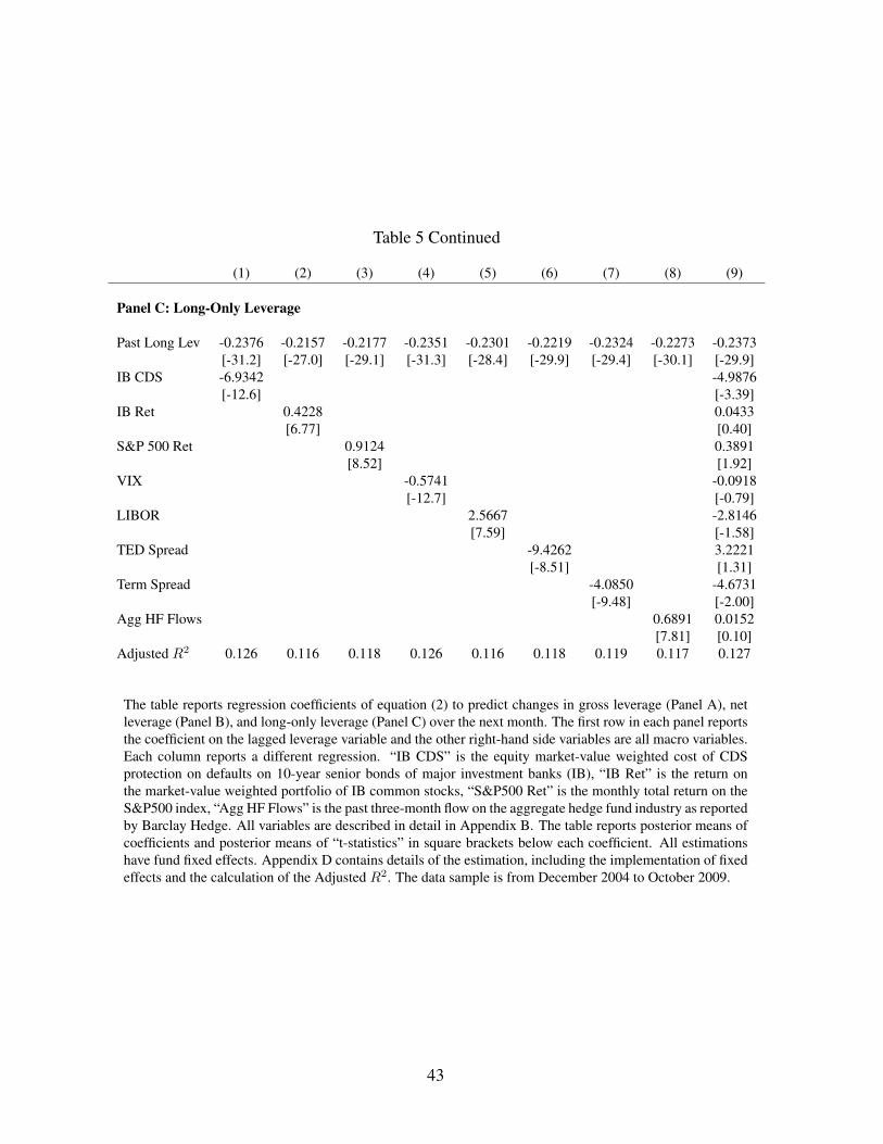
Table 5 Continued
(1) (2) (3) (4) (5) (6) (7) (8) (9)
Panel C: Long-Only Leverage
Past Long Lev -0.2376 -0.2157 -0.2177 -0.2351 -0.2301 -0.2219 -0.2324 -0.2273 -0.2373[-31.2] [-27.0] [-29.1] [-31.3] [-28.4] [-29.9] [-29.4] [-30.1] [-29.9]
IB CDS -6.9342 -4.9876[-12.6] [-3.39]
IB Ret 0.4228 0.0433[6.77] [0.40]
S&P 500 Ret 0.9124 0.3891[8.52] [1.92]
VIX -0.5741 -0.0918[-12.7] [-0.79]
LIBOR 2.5667 -2.8146[7.59] [-1.58]
TED Spread -9.4262 3.2221[-8.51] [1.31]
Term Spread -4.0850 -4.6731[-9.48] [-2.00]
Agg HF Flows 0.6891 0.0152[7.81] [0.10]
Adjusted R2 0.126 0.116 0.118 0.126 0.116 0.118 0.119 0.117 0.127
The table reports regression coefficients of equation (2) to predict changes in gross leverage (Panel A), netleverage (Panel B), and long-only leverage (Panel C) over the next month. The first row in each panel reportsthe coefficient on the lagged leverage variable and the other right-hand side variables are all macro variables.Each column reports a different regression. “IB CDS” is the equity market-value weighted cost of CDSprotection on defaults on 10-year senior bonds of major investment banks (IB), “IB Ret” is the return onthe market-value weighted portfolio of IB common stocks, “S&P500 Ret” is the monthly total return on theS&P500 index, “Agg HF Flows” is the past three-month flow on the aggregate hedge fund industry as reportedby Barclay Hedge. All variables are described in detail in Appendix B. The table reports posterior means ofcoefficients and posterior means of “t-statistics” in square brackets below each coefficient. All estimationshave fund fixed effects. Appendix D contains details of the estimation, including the implementation of fixedeffects and the calculation of the Adjusted R2. The data sample is from December 2004 to October 2009.
43

Table 6: Fund-Specific Predictors of Hedge Fund Leverage
(1) (2) (3) (4) (5)
Panel A: Gross Leverage
Past Gross Lev -0.2443 -0.2452 -0.2445 -0.2451 -0.2455[-30.3] [-30.5] [-30.5] [-30.1] [-31.1]
Past Ret -0.1288 -0.2151[-0.49] [-0.82]
12-month Vol -1.337 -1.4139[-1.93] [-2.11]
3-month Flows -0.0053 -0.0024[-0.21] [-0.10]
Log AUM -0.0325 -0.0414[-1.13] [-1.43]
Adjusted R2 0.130 0.131 0.131 0.131 0.131
Panel B: Net Leverage
Past Net Lev -0.3107 -0.3066 -0.3106 -0.3089 -0.3098[-3.69] [-3.99] [-3.59] [-3.71] [-3.62]
Past Ret -0.2357 -0.2057[-1.93] [-1.64]
12-month Vol 0.1615 0.0543[0.51] [0.18]
3-month Flows 0.0142 0.0153[1.35] [1.49]
Log AUM -0.0183 -0.0201[-1.41] [-1.45]
Adjusted R2 0.157 0.156 0.156 0.157 0.157
Panel C: Long-Only Leverage
Past Long Lev -0.2371 -0.2372 -0.2373 -0.2381 -0.2375[-30.4] [-32.1] [-31.1] [-29.9] [-30.6]
Past Ret -0.1923 -0.2258[-1.20] [-1.41]
12-month Vol -0.6278 -0.7289[-1.60] [-1.76]
3-month Flows 0.0048 0.0045[0.33] [0.31]
Log AUM -0.0236 -0.0284[-1.38] [-1.60]
Adjusted R2 0.127 0.127 0.127 0.127 0.127
44

Note to Table 6The table reports regression coefficients of equation (2) to predict changes in gross leverage (Panel A), netleverage (Panel B), and long-only leverage (Panel C) over the next month. The first row in each panel reportsthe coefficient on the lagged leverage variable and the other right-hand side variables are fund-specific andmacro variables. Each column reports a different regression. “Past Ret” is the fund’s return in the past month,“12-month Vol” is the volatility of the hedge fund’s returns computed using monthly data over the past 12months, “3-month Flows” is the hedge fund flow over the past three months computed using equation (1),and “Log AUM” is the logarithm of each hedge fund’s AUM. All the regression specifications also controlfor the macro predictors used in Table 5: the cost of CDS protection on major investment banks, the return onthe market-value weighted portfolio of investment banks, the S&P500 return, option VIX volatility, LIBOR,the TED spread, the term spread, and aggregate hedge fund flows. All variables are described in detail inAppendix B. The table reports posterior means of coefficients and posterior means of “t-statistics” in squarebrackets below each coefficient. All estimations have fund fixed effects. Appendix D contains details of theestimation, including the implementation of fixed effects and the calculation of the Adjusted R2. The datasample is from December 2004 to October 2009.
45

Table 7: Contemporaneous Relations with Gross Hedge Fund Leverage
Predictive Contemporaneous Predictive Contemporaneous
Macro Variables Fund-Specific Variables
Past Leverage -0.2447 Past Leverage -0.2455[-32.0] [-31.1]
IB CDS -9.3278 -1.3666 Past Ret -0.2151 -0.1123[-3.54] [-0.38] [-0.82] [-0.35]
IB Ret -0.0436 -0.2248 12-month Vol -1.4139 -4.3495[-0.26] [-0.90] [-2.11] [-2.35]
S&P 500 Ret 0.6750 -0.9419 3-month Flows -0.0024 -0.0530[2.09] [-2.02] [-0.10] [-1.11]
VIX -0.1010 -1.4324 Log AUM -0.0414 0.2552[-0.51] [-4.79] [-1.43] [1.75]
LIBOR -6.6629 3.4420[-2.35] [0.76]
TED Spread 7.5973 8.7629[1.90] [1.49]
Term Spread -10.32 -12.237[-2.80] [-2.09]
Agg HF Flows 0.0934 1.3419[0.38] [3.13]
ϕϵ 0.2494 ϕϵ 0.5547[32.9] [45.5]
Adjusted R2 0.131 0.080 Adjusted R2 0.131 0.086
The table reports regression coefficients for macro and fund-specific variables of the “Predictive” model inequation (2) and the “Contemporaneous” model in equation (3) for gross hedge fund leverage. The predictivemodel coefficients are identical to regression (9) of Table 5 for the macro-only predictors and regressionregression (5) of Table 6 for the fund-specific predictors. The “Fund-Specific Variables” regressions controlfor the macro predictors listed in the “Macro Variables” regressions: “IB CDS” is the equity market-valueweighted cost of CDS protection on defaults on 10-year senior bonds of major investment banks (IB), “IBRet” is the return on the market-value weighted portfolio of IB common stocks, “S&P500 Ret” is the monthlytotal return on the S&P500 index, “Agg HF Flows” is the past three-month flow on the aggregate hedge fundindustry as reported by Barclay Hedge. “Return” is the fund’s return in the last month, “12-month Vol” isthe volatility of the hedge fund’s returns computed using monthly data over the past 12 months includingthe last month, “3-month Flows” is the hedge fund flow over the past three months including the last monthcomputed using equation (1), and “Log AUM” is the logarithm of each hedge fund’s AUM. For the fund-specific variables: “Past Ret” is the fund’s return in the past month, “12-month Vol” is the volatility of thehedge fund’s returns computed using monthly data over the past 12 months, “3-month Flows” is the hedgefund flow over the past three months computed using equation (1), and “Log AUM” is the logarithm of eachhedge fund’s AUM. All variables are described in detail in Appendix B. The table reports posterior meansof coefficients and posterior means of “t-statistics” in square brackets below each coefficient. All estimationshave fund fixed effects. Appendix D contains details of the estimation, including the implementation of fixedeffects and the calculation of the Adjusted R2. The data sample is from December 2004 to October 2009.
46
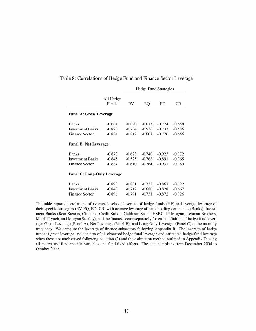
Table 8: Correlations of Hedge Fund and Finance Sector Leverage
Hedge Fund Strategies
All HedgeFunds RV EQ ED CR
Panel A: Gross Leverage
Banks -0.884 -0.820 -0.613 -0.774 -0.658Investment Banks -0.823 -0.734 -0.536 -0.733 -0.586Finance Sector -0.884 -0.812 -0.608 -0.776 -0.656
Panel B: Net Leverage
Banks -0.873 -0.623 -0.740 -0.923 -0.772Investment Banks -0.845 -0.525 -0.766 -0.891 -0.765Finance Sector -0.884 -0.610 -0.764 -0.931 -0.789
Panel C: Long-Only Leverage
Banks -0.893 -0.801 -0.735 -0.867 -0.722Investment Banks -0.840 -0.712 -0.680 -0.828 -0.667Finance Sector -0.896 -0.791 -0.738 -0.872 -0.726
The table reports correlations of average levels of leverage of hedge funds (HF) and average leverage oftheir specific strategies (RV, EQ, ED, CR) with average leverage of bank holding companies (Banks), Invest-ment Banks (Bear Stearns, Citibank, Credit Suisse, Goldman Sachs, HSBC, JP Morgan, Lehman Brothers,Merrill Lynch, and Morgan Stanley), and the finance sector separately for each definition of hedge fund lever-age: Gross Leverage (Panel A), Net Leverage (Panel B), and Long-Only Leverage (Panel C) at the monthlyfrequency. We compute the leverage of finance subsectors following Appendix B. The leverage of hedgefunds is gross leverage and consists of all observed hedge fund leverage and estimated hedge fund leveragewhen these are unobserved following equation (2) and the estimation method outlined in Appendix D usingall macro and fund-specific variables and fund-fixed effects. The data sample is from December 2004 toOctober 2009.
47

Table A-1: A Sample Hedge Fund Risk Exposure Report
Gross Leverage Net Leverage Long Market Value/ Short Market Value/Sector Ratio (%) Ratio (%) Equity (%) Equity (%)
Consumer Discretionary 16.73 1.93 9.33 (7.40)Consumer Staples 9.08 5.16 7.12 (1.96)Energy 7.84 (1.91) 2.97 (4.87)Financials 4.20 (2.87) 0.66 (3.53)Health Care 5.01 2.17 3.59 (1.42)Industrials 22.14 7.28 14.71 (7.43)Information Technology 26.05 5.41 15.73 (10.32)Materials 1.31 0.46 0.89 (0.43)Other Assets 17.72 3.76 10.74 (6.98)Telecommunication Services 0.69 0.28 0.48 (0.21)
Total 110.78 21.68 66.23 (44.55)
This table shows a sample hedge fund risk exposure report. This fund reports exposures monthly brokendown by sector. The reported quantities are percentages of NAV.
48
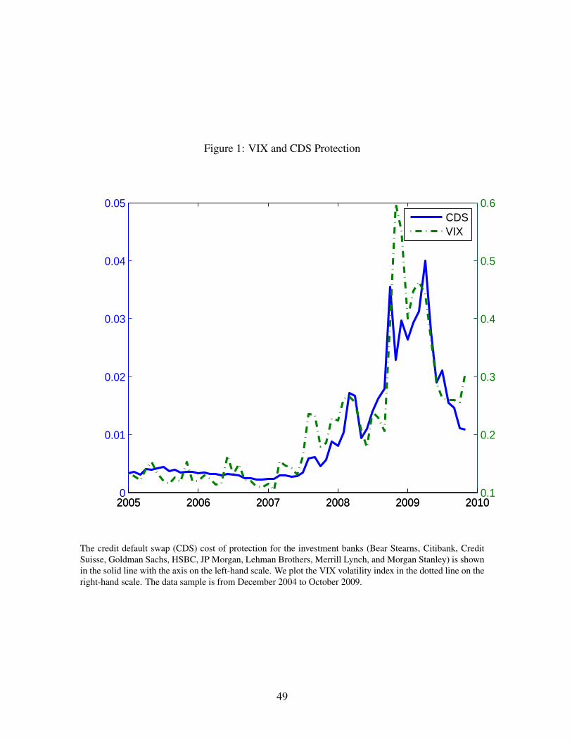
Figure 1: VIX and CDS Protection
2005 2006 2007 2008 2009 20100
0.01
0.02
0.03
0.04
0.05
2005 2006 2007 2008 2009 20100.1
0.2
0.3
0.4
0.5
0.6CDSVIX
The credit default swap (CDS) cost of protection for the investment banks (Bear Stearns, Citibank, CreditSuisse, Goldman Sachs, HSBC, JP Morgan, Lehman Brothers, Merrill Lynch, and Morgan Stanley) is shownin the solid line with the axis on the left-hand scale. We plot the VIX volatility index in the dotted line on theright-hand scale. The data sample is from December 2004 to October 2009.
49

Figure 2: Rolling 12-month Hedge Fund Volatilities
2005 2006 2007 2008 2009 20100
0.01
0.02
0.03
0.04
0.05
0.06
HFRVEQEDCR
This figure compares volatilities of returns of different hedge fund strategies over the sample period. Themonthly volatility for each strategy is constructed as an average value of sample volatilities of returns overthe past 12 months for the hedge funds that belong to the strategy. The strategies are relative value (RV),equity (EQ), event driven (ED), credit (CR), and the whole hedge fund sample is denoted HF. The datasample is from December 2004 to October 2009.
50

Figure 3: Hedge Fund Volatilities vs. HFR Volatilities
2005 2006 2007 2008 2009 20100.01
0.02
0.03
0.04
0.05
0.06
0.07
0.08
0.09
25−th percentile of volatility in HFRMedian volatility in HFR75−th percentile of volatility in HFRAverage volatility in the data sample
We plot 25-th, 50-th and 75-th percentile values of 12-month rolling volatilities of returns of funds in theHFR database and the average 12-month rolling volatility of returns of funds in the Fund’s database. Thedata sample is from December 2004 to October 2009.
51

Figure 4: Hedge Fund Gross Leverage
2005 2006 2007 2008 2009 20100
1
2
3
4
5
6
7
HFRVEQEDCR
The figure plots hedge fund gross leverage for all hedge funds (HF) and hedge fund sectors. The sectors arerelative value (RV), equity (EQ), event driven (ED), and credit (CR). The leverage aggregates all observedhedge fund leverage and estimated hedge fund leverage when these are unobserved following the estimationmethod outlined in Appendix D. These estimates are obtained using the model in equation (2) using all macroand fund-specific variables and fund-fixed effects. The data sample is from December 2004 to October 2009.
52
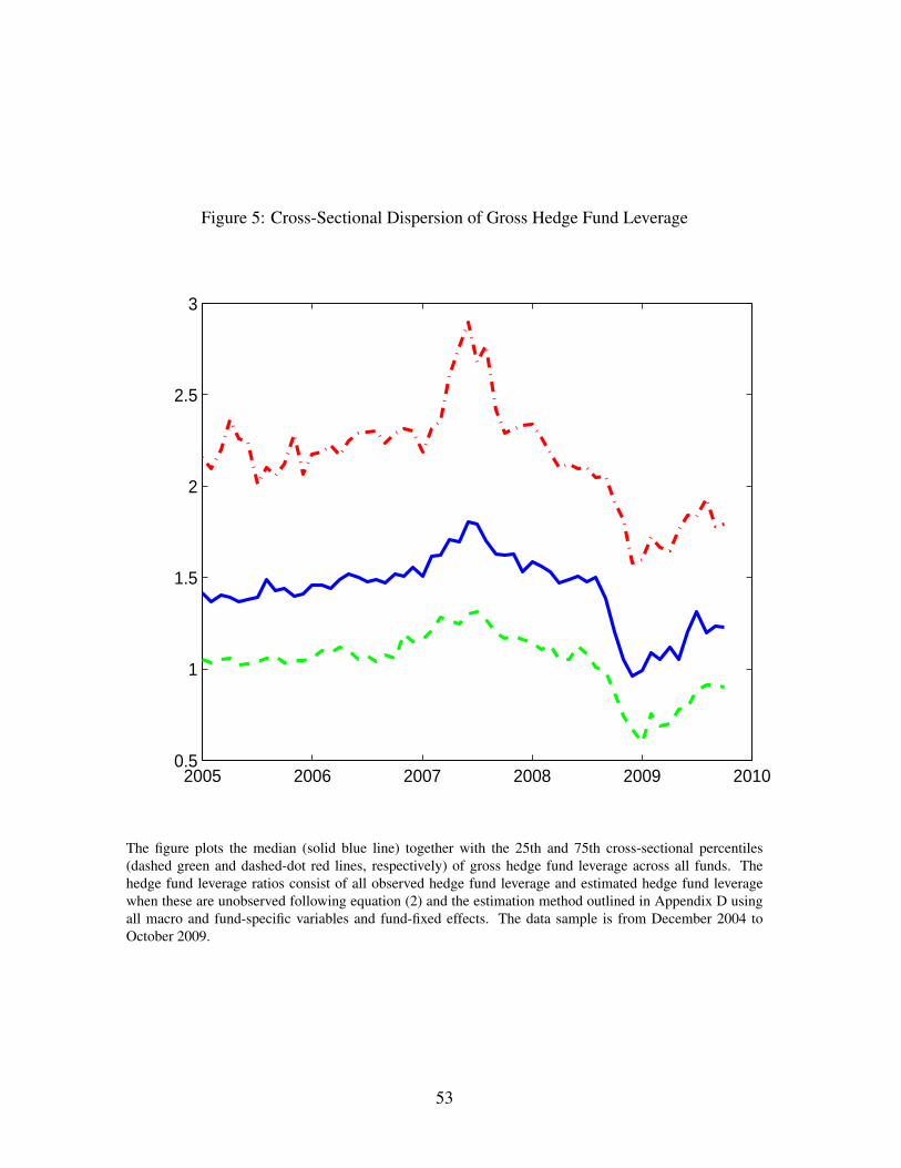
Figure 5: Cross-Sectional Dispersion of Gross Hedge Fund Leverage
2005 2006 2007 2008 2009 20100.5
1
1.5
2
2.5
3
The figure plots the median (solid blue line) together with the 25th and 75th cross-sectional percentiles(dashed green and dashed-dot red lines, respectively) of gross hedge fund leverage across all funds. Thehedge fund leverage ratios consist of all observed hedge fund leverage and estimated hedge fund leveragewhen these are unobserved following equation (2) and the estimation method outlined in Appendix D usingall macro and fund-specific variables and fund-fixed effects. The data sample is from December 2004 toOctober 2009.
53
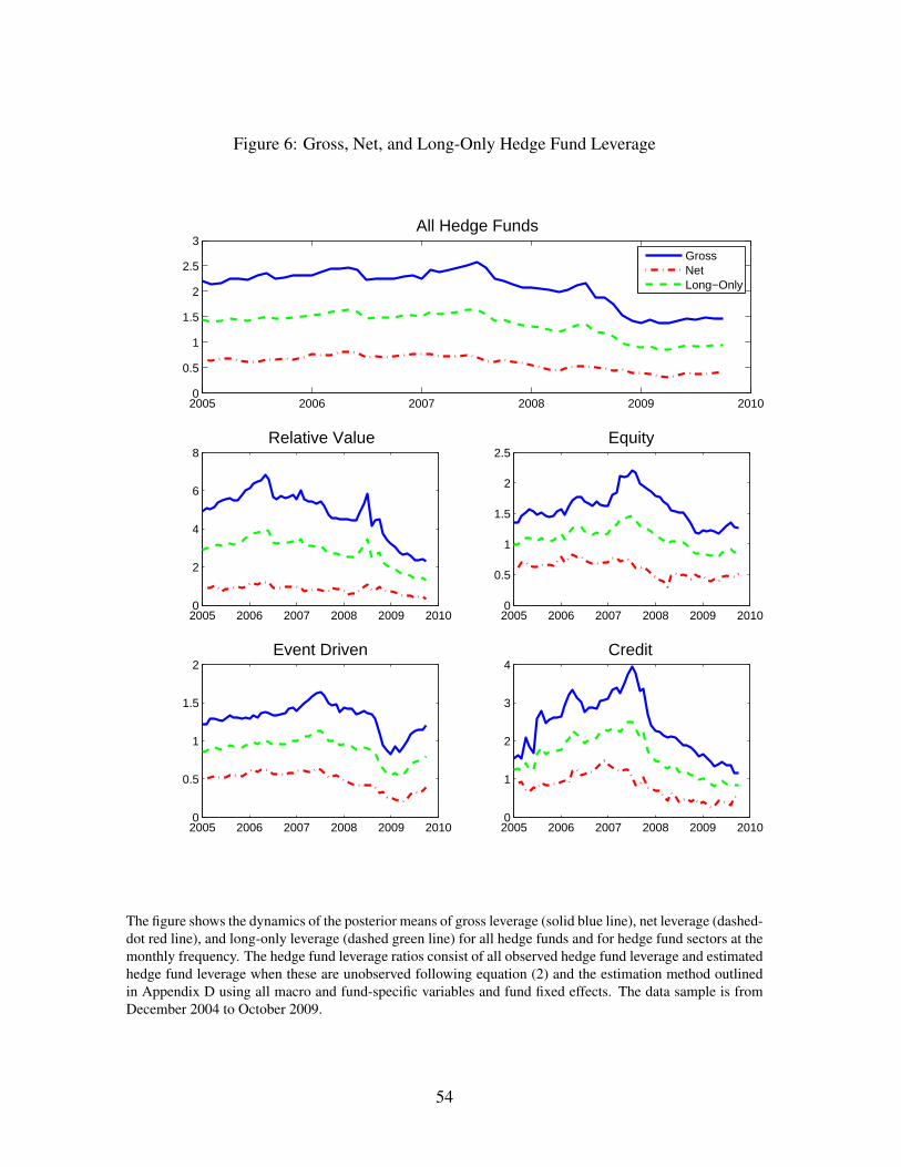
Figure 6: Gross, Net, and Long-Only Hedge Fund Leverage
2005 2006 2007 2008 2009 20100
0.5
1
1.5
2
2.5
3All Hedge Funds
GrossNetLong−Only
2005 2006 2007 2008 2009 20100
2
4
6
8Relative Value
2005 2006 2007 2008 2009 20100
0.5
1
1.5
2
2.5Equity
2005 2006 2007 2008 2009 20100
0.5
1
1.5
2Event Driven
2005 2006 2007 2008 2009 20100
1
2
3
4Credit
The figure shows the dynamics of the posterior means of gross leverage (solid blue line), net leverage (dashed-dot red line), and long-only leverage (dashed green line) for all hedge funds and for hedge fund sectors at themonthly frequency. The hedge fund leverage ratios consist of all observed hedge fund leverage and estimatedhedge fund leverage when these are unobserved following equation (2) and the estimation method outlinedin Appendix D using all macro and fund-specific variables and fund fixed effects. The data sample is fromDecember 2004 to October 2009.
54

Figure 7: Hedge Fund and Finance Sector Leverage
2005 2006 2007 2008 2009 20100
0.5
1
1.5
2
2.5
3
0
10
20
30
40
50
Hedge FundsBanksInvestment BanksFinance Sector
We compare average gross hedge fund leverage with the leverage of banks, investment banks, and the financesector. The left-hand axis corresponds to average gross hedge fund leverage and the right-hand axis corre-sponds to the leverage of banks, investment banks, and the finance sector. The hedge fund leverage ratiosconsist of all observed hedge fund leverage and estimated hedge fund leverage when these are unobservedfollowing equation (2) and the estimation method outlined in Appendix D using all macro and fund-specificvariables and fund-fixed effects. The finance sector leverage is constructing following the method describedin Appendix B. The data sample is from December 2004 to October 2009.
55

Figure 8: Hedge Fund and Investment Bank Gross Exposure and Leverage
Hedge Funds
2005 2006 2007 2008 2009 20101
2
3
4
5
6
1
1.5
2
2.5Hedge Fund ExposureHedge Fund AUM
Investment Banks
2005 2006 2007 2008 2009 20103
4
5
6
7
8
0
0.1
0.2
0.3
0.4
0.5
0.6
0.7
0.8IB AssetsIB Market Value
56

Note to Figure 8We graph the gross exposure and AUM of hedge funds in Panel A and the gross exposure and market valueof equity of investment banks (IB) in Panel B. For hedge funds, we take gross leverage across all hedgefunds which consists of observed gross leverage and estimated gross leverage when these are unobservedfollowing equation (2) and the estimation method outlined in Appendix D using all macro and fund-specificvariables and fund fixed effects. The hedge fund exposure is computed by multiplying the gross leverage bythe aggregated AUM of hedge funds from the Barclays Hedge database. Investment bank exposure is the totalamount of assets held by investment banks. The left-hand axes in both panels correspond to AUM or equity.The market value of investment banks is the value of common equity. Appendix B contains further detailson these variables. The right-hand axes correspond to gross exposure. The scale of both axes is in trillions ofdollars. The data sample is from December 2004 to October 2009.
57

Figure 9: Relative Gross Exposures of Hedge Funds to Investment Banks and the Finance Sector
2005 2006 2007 2008 2009 20100.3
0.4
0.5
0.6
0.7
0.8
2005 2006 2007 2008 2009 20100.1
0.15
0.2
0.25
0.3
0.35
Relative exposure of HF to IB assetsRelative exposure of HF to FS assets
We plot the ratio of gross exposure of hedge funds (HF) to investment banks (IB) and the finance sector (FS).The gross exposure is computed by multiplying gross leverage and AUM in the case of hedge funds and istotal assets in the case of investment banks and the finance sector. For hedge funds, we take gross leverageacross all hedge funds which consists of observed gross leverage and estimated gross leverage when theseare unobserved following the estimation method outlined in Appendix D using all macro and fund-specificvariables and fund fixed effects. The left-hand axis corresponds to the relative gross exposure of hedge fundsto the assets of investment banks, while the right-hand axis corresponds to the relative exposure of hedgefunds to the assets of the finance sector. The data sample is from December 2004 to October 2009.
58
Top Related