


![LECT06 - MDOF Part 2 [Compatibility Mode]](https://static.fdocuments.us/doc/165x107/577cc1431a28aba711928c4a/lect06-mdof-part-2-compatibility-mode.jpg)


Languages
Pages
Legal


MEEN 617 HD 11 Modal Analysis of MDOF Systems with Viscous Damping L. San Andrés © 2013
1
MEEN 617 Handout #11
MODAL ANALYSIS OF MDOF Systems with VISCOUS DAMPING ^ Symmetric
The motion of a n-DOF linear system is described by the set of 2nd
order differential equations
( )tM U + CU + K U = F
(1)
where U(t) and F(t) are n rows vectors of displacements and external
forces, respectively. M, K, C are the system (nxn) matrices of mass,
stiffness, and viscous damping coefficients. These matrices are
symmetric, i.e. M=MT, K=KT, C=CT.
The solution to Eq. (1) is determined uniquely if vectors of initial
displacements Uo and initial velocities 0t
dd t
oUV are specified.
For free vibrations, the force vector F(t)=0 , and Eq. (1) is
M U +CU + K U = 0 (2)
A solution to Eq. (2) is of the form
teU ψ (3)
where in general is a complex number. Substitution of Eq. (3) into
Eq. (2) leads to the following characteristic equation:
2 0 M C K Ψ f Ψ (4)
MEEN 617 HD 11 Modal Analysis of MDOF Systems with Viscous Damping L. San Andrés © 2013
2
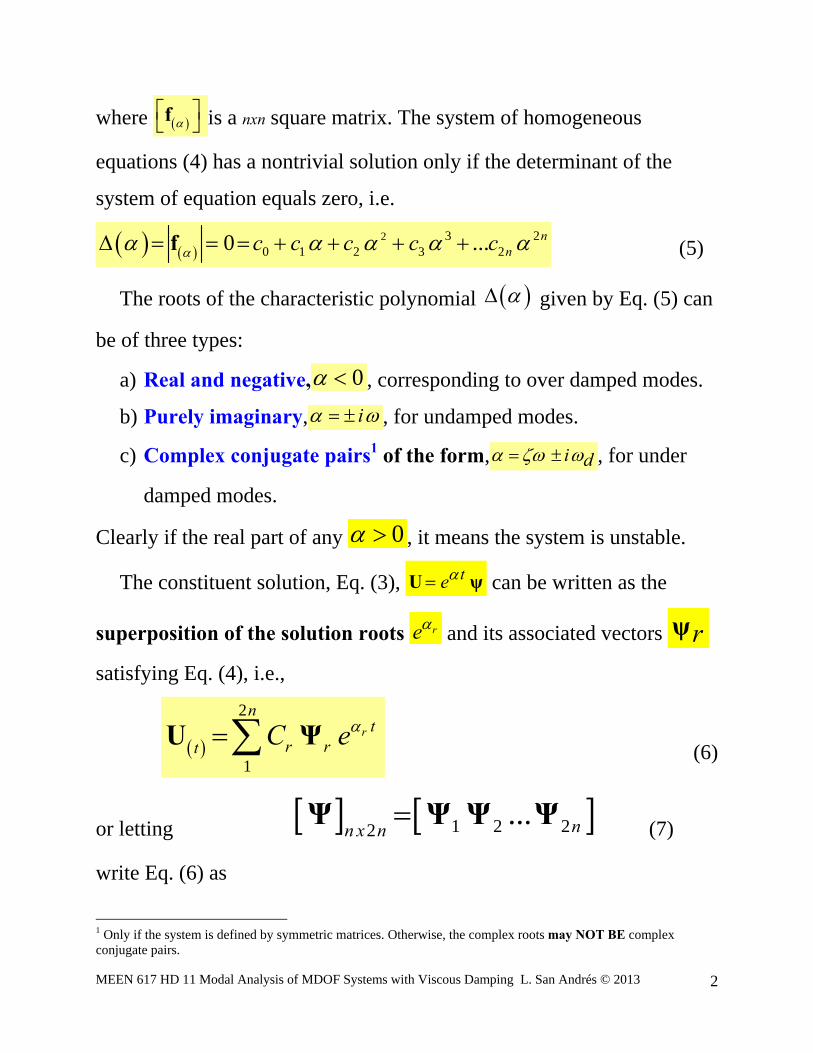
where f is a nxn square matrix. The system of homogeneous
equations (4) has a nontrivial solution only if the determinant of the
system of equation equals zero, i.e.
2 3 2
0 1 2 3 20 ... nnc c c c c f (5)
The roots of the characteristic polynomial given by Eq. (5) can
be of three types:
a) Real and negative, 0 , corresponding to over damped modes.
b) Purely imaginary, i , for undamped modes.
c) Complex conjugate pairs1 of the form, i d , for under
damped modes.
Clearly if the real part of any 0 , it means the system is unstable.
The constituent solution, Eq. (3), teU ψ can be written as the
superposition of the solution roots re and its associated vectors rψ
satisfying Eq. (4), i.e.,
2
1
r
nt
r rt C eU Ψ (6)
or letting 1 2 22... nn x n
Ψ Ψ Ψ Ψ (7)
write Eq. (6) as
1 Only if the system is defined by symmetric matrices. Otherwise, the complex roots may NOT BE complex conjugate pairs.

MEEN 617 HD 11 Modal Analysis of MDOF Systems with Viscous Damping L. San Andrés © 2013
3
r trt C eU Ψ (8)
However, a transformation of the form,
2 11
nxnx tU Ψ q (9)
is not possible since this implies the existence of 2n- modal coordinates
which is not physically apparent when the number of physical
coordinates is only n.
To overcome this apparent difficulty, reformulate the problem in a
slightly different form. Let Y be a 2n- rows vector composed of the
physical velocities and displacements, i.e.
UY =
U
, and (t)
0Q =
F (10)
be a modified force vector. Then write tM U +CU + K U = F as
0 M -M 0U U 0+ =U FUM C 0 K
(11.a)
or
A Y + B Y = Q (11.b)
where
0 M -M 0A = , B =
M C 0 K (12)
MEEN 617 HD 11 Modal Analysis of MDOF Systems with Viscous Damping L. San Andrés © 2013
4
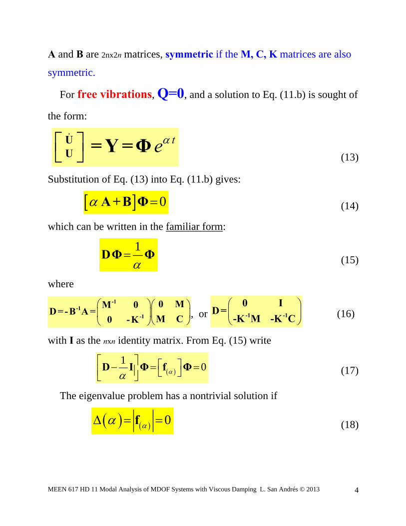
A and B are 2nx2n matrices, symmetric if the M, C, K matrices are also
symmetric.
For free vibrations, Q=0, and a solution to Eq. (11.b) is sought of
the form:
te UU = Y =Φ
(13)
Substitution of Eq. (13) into Eq. (11.b) gives:
0 A +B Φ (14)
which can be written in the familiar form:
1
DΦ Φ (15)
where
-1-1
-1
0 MM 0D= -B A =
M C0 -K, or
-1 -1
0 ID=
-K M -K C (16)
with I as the nxn identity matrix. From Eq. (15) write
1
0 D Ι Φ f Φ (17)
The eigenvalue problem has a nontrivial solution if
0 f (18)
MEEN 617 HD 11 Modal Analysis of MDOF Systems with Viscous Damping L. San Andrés © 2013
5
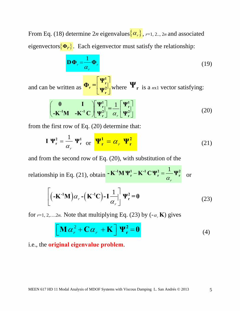
From Eq. (18) determine 2n eigenvalues r , r=1, 2.., 2n and associated
eigenvectors rΦ . Each eigenvector must satisfy the relationship:
1
r rr
DΦ Φ (19)
and can be written as
1r
r 2r
ΨΦ =
Ψ where rΨ is a nx1 vector satisfying:
1
r
1 1r r
-1 -1 2 2r r
0 I Ψ Ψ=
-K M -K C Ψ Ψ (20)
from the first row of Eq. (20) determine that:
1
r2 1
r rI Ψ Ψ or r1 2r rΨ Ψ (21)
and from the second row of Eq. (20), with substitution of the
relationship in Eq. (21), obtain1
r -1 1 -1 2 2
r r r- K MΨ K CΨ Ψ or
1r
r
-1 -1 2r-K M - K C -I Ψ = 0 (23)
for r=1, 2,….2n. Note that multiplying Eq. (23) by (- r K) gives
2r r
2rM C K Ψ 0 (4)
i.e., the original eigenvalue problem.
MEEN 617 HD 11 Modal Analysis of MDOF Systems with Viscous Damping L. San Andrés © 2013
6
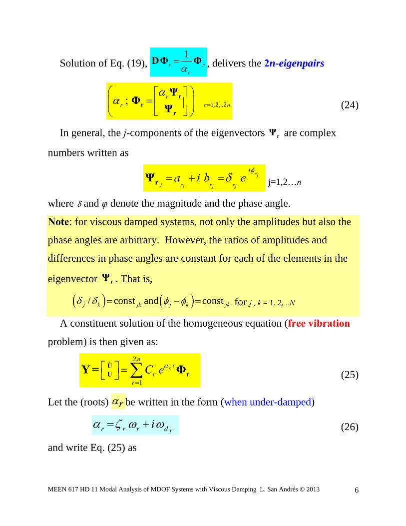
Solution of Eq. (19), 1
r rr
DΦ Φ , delivers the 2n-eigenpairs
1,2,..2; rr r n
rr
r
ΨΦ
Ψ (24)
In general, the j-components of the eigenvectors rΨ are complex
numbers written as
rj
j r r rj j j
ia i b e
rΨ j=1,2…n
where and φ denote the magnitude and the phase angle.
Note: for viscous damped systems, not only the amplitudes but also the
phase angles are arbitrary. However, the ratios of amplitudes and
differences in phase angles are constant for each of the elements in the
eigenvector rΨ . That is,
/ const and constj k jk j k jk for j , k = 1, 2, ..N
A constituent solution of the homogeneous equation (free vibration
problem) is then given as:
2
1
r
nt
rr
C e
UU rY = Φ
(25)
Let the (roots) r be written in the form (when under-damped)
r r r d ri (26)
and write Eq. (25) as
MEEN 617 HD 11 Modal Analysis of MDOF Systems with Viscous Damping L. San Andrés © 2013
7
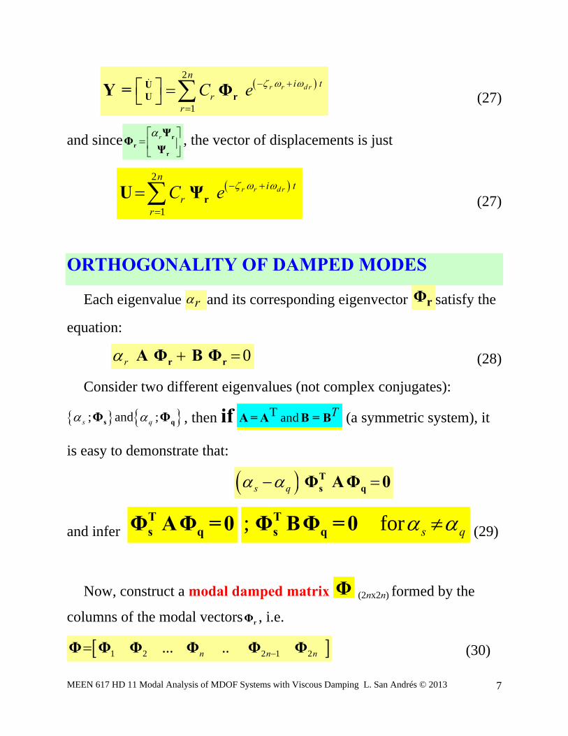
2
1
r r d r
ni t
rr
C e
UU rY = Φ
(27)
and since r
rr
r
ΨΦ
Ψ, the vector of displacements is just
2
1
r r d r
ni t
rr
C e
rU Ψ (27)
ORTHOGONALITY OF DAMPED MODES
Each eigenvalue r and its corresponding eigenvector rΦ satisfy the
equation:
0r r rΑ Φ B Φ (28)
Consider two different eigenvalues (not complex conjugates):
; and ;s q s qΦ Φ , then if T and TΑ =Α B = B (a symmetric system), it
is easy to demonstrate that:
s q Ts qΦ AΦ 0
and infer Ts qΦ AΦ =0 ; for s q T
s qΦ ΒΦ = 0 (29)
Now, construct a modal damped matrix Φ (2nx2n) formed by the
columns of the modal vectors rΦ , i.e.
1 2 2 1 2... ..n n nΦ Φ Φ Φ Φ Φ (30)
MEEN 617 HD 11 Modal Analysis of MDOF Systems with Viscous Damping L. San Andrés © 2013
8
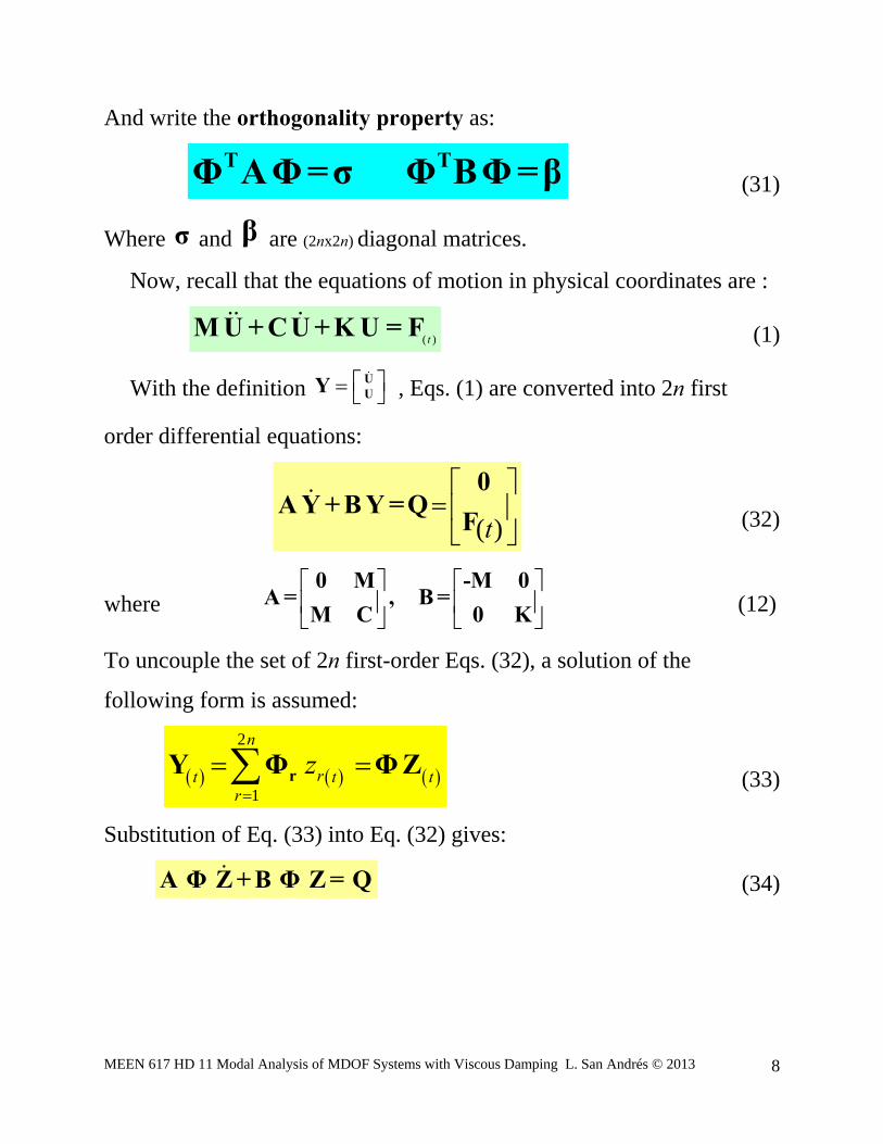
And write the orthogonality property as:
T TΦ ΑΦ=σ Φ ΒΦ=β (31)
Where σ and β are (2nx2n) diagonal matrices.
Now, recall that the equations of motion in physical coordinates are :
( )tM U + CU + K U = F
(1)
With the definition UUY
, Eqs. (1) are converted into 2n first
order differential equations:
( )t
0ΑY +ΒY =Q
F
(32)
where
0 M -M 0A = , B =
M C 0 K (12)
To uncouple the set of 2n first-order Eqs. (32), a solution of the
following form is assumed:
2
1
n
rt t tr
z
rY Φ ΦZ (33)
Substitution of Eq. (33) into Eq. (32) gives:
Α Φ Ζ+Β Φ Ζ= Q (34)

MEEN 617 HD 11 Modal Analysis of MDOF Systems with Viscous Damping L. San Andrés © 2013
9
Premultiply this equation by TΦ and use the orthogonality property2 of
the damped modes to get:
T T TΦ Α Φ Ζ+ Φ Β Φ Ζ=Φ Q (35)
or Tσ Ζ+β Ζ= G Φ Q (36)
Eq. (36) represents a set of 2n uncoupled first order equations:
( )1 1 1 1 1 tz z g
( )2 2 2 2 2 tz z g
( )2 2 2 2 2 tN N N N Nz z g (37)
where ;r r r r T Tr r r rΦ ΑΦ Φ BΦ , r=1, 2..2N
/r r r (38)
since r r rΑΦ Β Φ 0 . In addition,
( ) ( )tr tg T
rΦ Q (39)
Initial conditions are also determined from o
oo
UUY
with the
transformation 0 0tY ΦZ
TσΖ =Φ ΑYo o (40.a)
2 The result below is only valid for symmetric systems, i.e. with M, K and C as symmetric matrices. For the more general case (non symmetric system), see the textbook of Meirovitch to find a discussion on LEFT and RIGHT eigenvectors.
MEEN 617 HD 11 Modal Analysis of MDOF Systems with Viscous Damping L. San Andrés © 2013
10
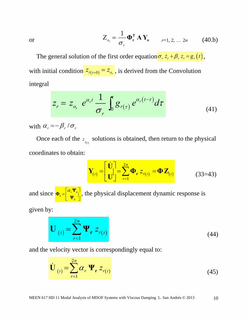
or 1
ror
Tr oΦ ΑY r=1, 2, 2n (40.b)
The general solution of the first order equation r r r r rz z g t ,
with initial condition 0 rr otz z , is derived from the Convolution
integral
0
1rr
r
t ttr o r
r
z z e g e d
(41)
with /r r r
Once each of the ( )r t
z solutions is obtained, then return to the physical
coordinates to obtain:
2
1
n
rt t tr
z
r
UY Φ ΦZ
U
(33=43)
and since r
rr
r
ΨΦ
Ψ, the physical displacement dynamic response is
given by:
2
1
n
rt tr
z
rU Ψ (44)
and the velocity vector is correspondingly equal to:
2
1
n
r rt tr
z
rU Ψ (45)

MEEN 617 HD 11 Modal Analysis of MDOF Systems with Viscous Damping L. San Andrés © 2013
11
Read/study the accompanying MATHCAD® worksheet with a detailed
example for discussion in class.

k3 2.0 107 n 3 # of DOF
Make matrices:
M
m1
0
0
0
m2
0
0
0
m3
K
k1 k2
k2
0
k2
k2 k3
k3
0
k3
k3
C
c1 c2
c2
0
c2
c2 c3
c3
0
c3
c3
Initial conditions in displacement and velocity:
PLOTs - only N 1024 # for time steps
Uo
1
0
0
Vo
0
.1
0
natural freqs - undamped
damped eigenvals
=====================================================================2. Evaluate the damped eigenvalues: Rewrite Eq (1), as
A dY/dt + B Y = Q(t), where Y = [ dU/dt, U ]T, and Q=[0, F(t)]T are 2n row vectors of (velocity, displacements ) and generalized forces; and initial conditions Yo = [ Vo, Uo ]
are 2nx2nSymmetric matricesA
0
M
M
C
= BM
0
0
K
=
MODAL ANALYSIS of MDOF linear systems with viscous dampingOriginal by Dr. Luis San Andres for MEEN 617 class / SP 08, 12
(1)The equations of motion are: M d2U/dt2 + C dU/dt + K U = F(t)where M,C,K are nxn SYMMETRIC matrices of inertia, viscous damping and stiffness coefficients, and U, dU/dt, d2U/dt2,and are the nx1 vectors of displacements, velocity and accelerations. F(t) is the nx1 vector of generalized forces. Eq (1) is solved with appropriate initial conditions, at t=0, Uo,Vo=dU/dt
========================================================================
Define elements of inertia, stiffness, and damping matrices:
m1 100 k1 1.0 107 c1 5000
m2 100 N/m N.s/mkg k2 1.0 107 c2 2000
m3 50 c3 1000
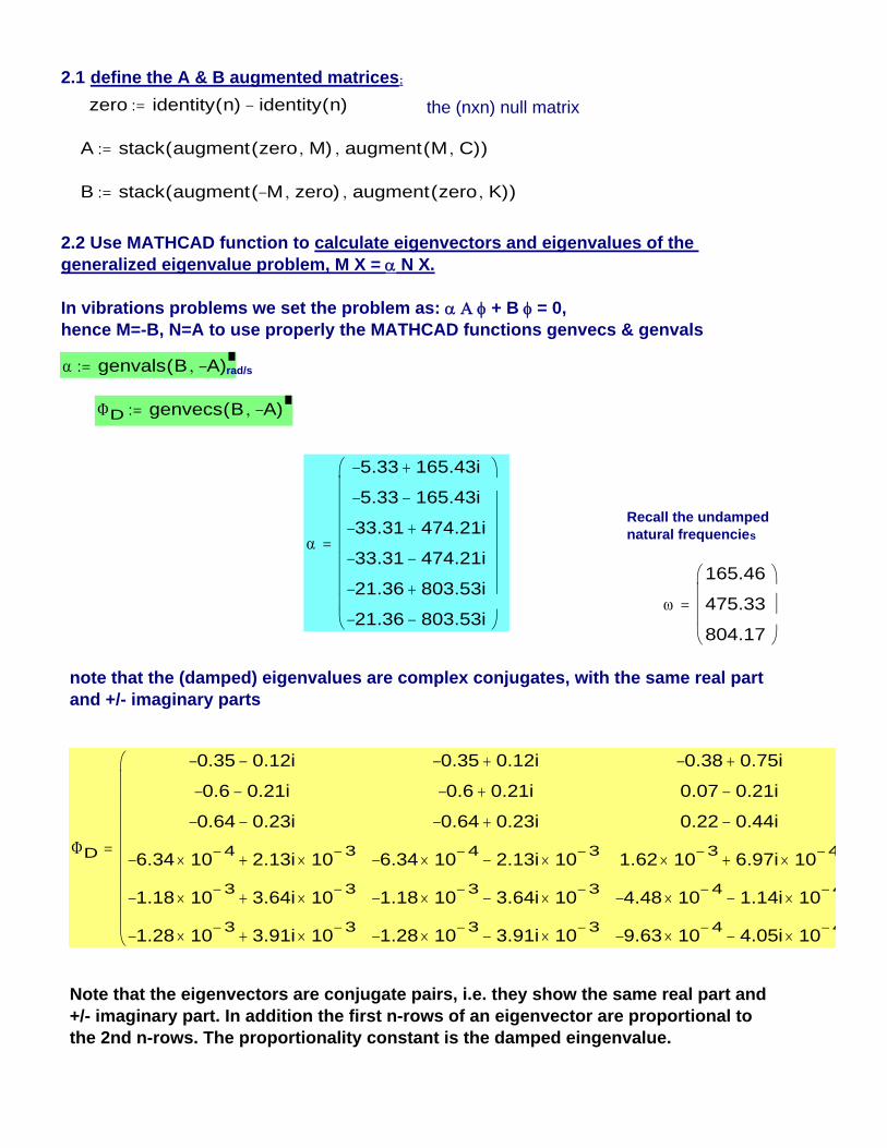
2.1 define the A & B augmented matrices:
zero identity n( ) identity n( ) the (nxn) null matrix
A stack augment zero M( ) augment M C( )( )
B stack augment M zero( ) augment zero K( )( )
2.2 Use MATHCAD function to calculate eigenvectors and eigenvalues of the generalized eigenvalue problem, M X = N X.
In vibrations problems we set the problem as: + B = 0,hence M=-B, N=A to use properly the MATHCAD functions genvecs & genvals
genvals B A( ) rad/s
D genvecs B A( )
Recall the undamped natural frequencies
5.33 165.43i
5.33 165.43i
33.31 474.21i
33.31 474.21i
21.36 803.53i
21.36 803.53i
165.46
475.33
804.17
note that the (damped) eigenvalues are complex conjugates, with the same real part and +/- imaginary parts
D
0.35 0.12i
0.6 0.21i
0.64 0.23i
6.34 104 2.13i 10
3
1.18 103 3.64i 10
3
1.28 103 3.91i 10
3
0.35 0.12i
0.6 0.21i
0.64 0.23i
6.34 104 2.13i 10
3
1.18 103 3.64i 10
3
1.28 103 3.91i 10
3
0.38 0.75i
0.07 0.21i
0.22 0.44i
1.62 103 6.97i 10
4
4.48 104 1.14i 10
4
9.63 104 4.05i 10
4
Note that the eigenvectors are conjugate pairs, i.e. they show the same real part and +/- imaginary part. In addition the first n-rows of an eigenvector are proportional to the 2nd n-rows. The proportionality constant is the damped eingenvalue.
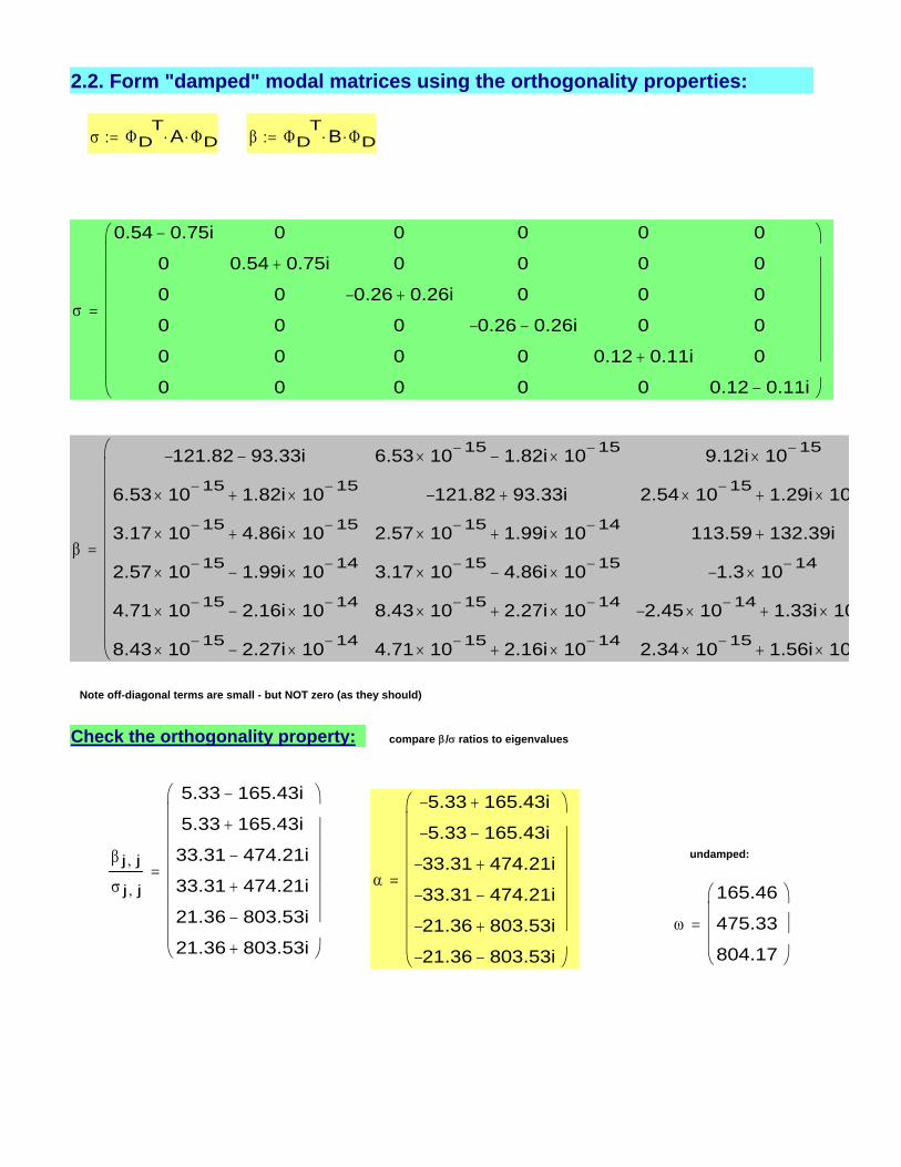
2.2. Form "damped" modal matrices using the orthogonality properties:
DT
A D DT
B D
0.54 0.75i
0
0
0
0
0
0
0.54 0.75i
0
0
0
0
0
0
0.26 0.26i
0
0
0
0
0
0
0.26 0.26i
0
0
0
0
0
0
0.12 0.11i
0
0
0
0
0
0
0.12 0.11i
121.82 93.33i
6.53 1015 1.82i 10
15
3.17 1015 4.86i 10
15
2.57 1015 1.99i 10
14
4.71 1015 2.16i 10
14
8.43 1015 2.27i 10
14
6.53 1015 1.82i 10
15
121.82 93.33i
2.57 1015 1.99i 10
14
3.17 1015 4.86i 10
15
8.43 1015 2.27i 10
14
4.71 1015 2.16i 10
14
9.12i 1015
2.54 1015 1.29i 10
113.59 132.39i
1.3 1014
2.45 1014 1.33i 10
2.34 1015 1.56i 10
Note off-diagonal terms are small - but NOT zero (as they should)
Check the orthogonality property: compare / ratios to eigenvalues
undamped: j j
j j
5.33 165.43i
5.33 165.43i
33.31 474.21i
33.31 474.21i
21.36 803.53i
21.36 803.53i
5.33 165.43i
5.33 165.43i
33.31 474.21i
33.31 474.21i
21.36 803.53i
21.36 803.53i
165.46
475.33
804.17

damped modal response
from undamped modal analysisT
165.46 475.33 804.17( )
dT
165.43 165.43 474.21 474.21 803.53 803.53( ) damped natural freqs.
rad/snatural freqs.nT
165.52 165.52 475.37 475.37 803.81 803.81( )
T
0.03 0.03 0.07 0.07 0.03 0.03( ) damping ratios.
damped eigenvals
damped natural freqs.
dj
Im j
natural frequenciesnj
Re j j
j1
Im j Re j
2
1
.5
j 1 2 n
d n 1 2
.5=damping ratios:imaginary part:
nreal part: for underdamped systems only
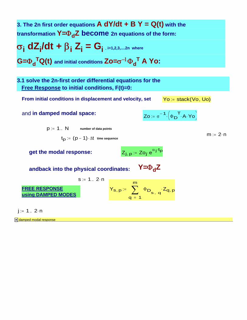
damped modal response
j 1 2 n
Ys p
1
m
q
Ds q
Zq p
FREE RESPONSEusing DAMPED MODES
s 1 2 n
andback into the physical coordinates: Y=dZ
Zj p Zoj e j tpget the modal response:
time sequencetp p 1( ) tm 2 n
number of data pointsp 1 N
Zo 1
DT
A Yo
and in damped modal space:
Yo stack Vo Uo( )From initial conditions in displacement and velocity, set
3.1 solve the 2n-first order differential equations for the Free Response to initial conditions, F(t)=0:
3. The 2n first order equations A dY/dt + B Y = Q(t) with the transformation Y=dZ become 2n equations of the form:
i dZi/dt + i Zi = Gi , i=1,2,3,....2n where
G=dTQ(t) and initial conditions Zo=d
T A Yo:

recall:Plot the displacements (last n rows of Y vector):Uo
1
0
0
RESPONSE: U1
0 0.022 0.043 0.065 0.087 0.11 0.13 0.151
0
1
dampedundamped
time(secs)
U1
RESPONSE: U2
0 0.022 0.043 0.065 0.087 0.11 0.13 0.151
0.5
0
0.5
1
DampedUndamped
time(secs)
U2
RESPONSE: U3
0 0.022 0.043 0.065 0.087 0.11 0.13 0.151
0
1
DampedUndamped
time(secs)
U3
T
0.03 0.03 0.07 0.07 0.03 0.03( )

and in physical coordinates:m 2 ns 1 m
Ys p
1
m
q
Ds q
Zq p
STEP RESPONSEusing DAMPED MODES
Y=dZ
===================================================================6. For completeness, obtain also the undamped forced response:
o Mm1
T M Uo o Mm
1 T
M Vo T
Fo
j 1 n
j p oj cos j tp oj
jsin j tp
j
Kmj j1 cos j tp
s 1 nand into physical coordinates:
STEP RESPONSEusing UNDAMPED MODES U Us p
1
n
q
s q q p
================================================================== static response - check
Us K1
FoPlot the displacements (last n rows of Y vector):Step load response
4. Forced response to step load F(t)=Fo and initial conditions Set initial conditions in displacement and velocity:
STEP FORCEFo
30000
105
105
O
0
0
0
Uo
0
0
0
Vo
0
0
0
Step load response
Then set: Yo stack Vo Uo( ) Qo stack O Fo( )
and transform to damped modal space: Zo 1
DT
A Yo
Go D
TQo
Tmax8
f1 secs t
Tmax
N j 1 2 n
p 1 Ntp p 1( ) t
to get the modal response Zj p Zoj e j tp
Goj
j j1 e
j tp
p p
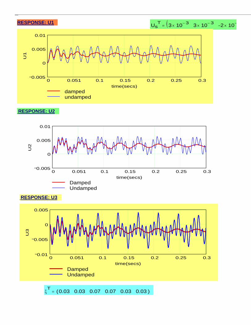
RESPONSE: U1Us
T3 10
3 3 103 2 10
0 0.051 0.1 0.15 0.2 0.25 0.30.005
0
0.005
0.01
dampedundamped
time(secs)
U1
RESPONSE: U2
0 0.051 0.1 0.15 0.2 0.25 0.30.005
0
0.005
0.01
DampedUndamped
time(secs)
U2
RESPONSE: U3
0 0.051 0.1 0.15 0.2 0.25 0.30.01
0.005
0
0.005
DampedUndamped
time(secs)
U3
T
0.03 0.03 0.07 0.07 0.03 0.03( )

0 01
0.005
0
0.005
0.01
U3
RESPONSE: U3
0 0.00560.01110.01670.02220.02780.03330.03890.0444 0.050.01
0
0.01
DampedUndamped
time(secs)
U2
RESPONSE: U2
j
165.46
475.33
804.17
0 0.00560.01110.01670.02220.02780.03330.03890.0444 0.050.02
0
0.02
dampedundamped
time(secs)
U1
RESPONSE: U1 502.65recall:
Plot the displacements (last n rows of Y vector):
502.65
165.46
475.33
804.17
recall theundampedfrequencies
2 fHzFo
3 104
1 105
1 105
fHz 80
freq. of excitationResponse due to initial conditions vanishes after a long time because of damping:
5. Periodic response to loading, F(t)=Fo sin(t):

qj k j
Kmj j
1
1.0k 2
j 2
2 jk
j
i
kmin 12.06
here i=imaginary unit
s 1 n
Us k
1
n
i
s i qi k
x cos(t)FRF in physical plane:
___________________________________________________________
DAMPED CASE set: Qo stack O Fo( )forcing vector
Go DT
Qo
k kmin kmax
kk
kmaxmax
rad/s <=== forcing frequency
j 1 2 n Zj kGoj
j j
1
1 ik
j
x cos(t)modal response
and back into the physical plane:
6) FRF Response to periodic loading, F=Fo cos(t)
UNDAMPED CASE
i 1 nSET
0
0
0
Fo
3 104
1 105
1 105
modal force magntidue:
TFo i
165.46
475.33
804.17
and the modal "S-S" response is modes.
j 1 n max 3 n
kmin 1 kmax 200
k kmin kmaxrad/sec <=== forcing frequency
kk
kmaxmax
kmax 2.41 103
x cos(t)MODALresponse

s 1 2 n m 2 n
PERIODIC RESPONSEusing DAMPED MODES
Ys k
1
m
q
Ds q
Zq k
x cos(t)
Plot magnitude of response in physical space
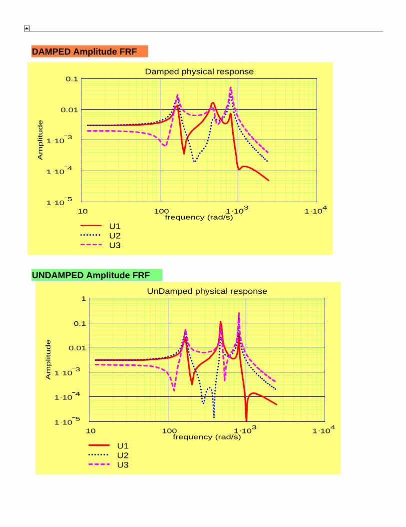
DAMPED Amplitude FRF
10 100 1 103
1 104
1 105
1 104
1 103
0.01
0.1
U1U2U3
Damped physical response
frequency (rad/s)
Am
plitu
de
UNDAMPED Amplitude FRF
10 100 1 103
1 104
1 105
1 104
1 103
0.01
0.1
1
U1U2U3
UnDamped physical response
frequency (rad/s)
Am
plitu
de

select coordinate to displate physical response - damped & undamped jj 2 n 3 DOFs
10 100 1 103
1 104
1 105
1 104
1 103
0.01
0.1
1
dampedundamped
frequency (rad/s)
LINEAR vertical scale undamped: T
165.46 475.33 804.17( )
10 100 1 103
1 104
0
0.05
0.1
0.15
0.2
dampedundamped
frequency (rad/s)
Top Related