


Languages
Pages
Legal


i
Harmonic Interaction between weak AC systems and VSC-based HVDC schemes
By
Ernst Krige
Thesis presented in fulfilment of the requirements for the degree
Master of Science in Electrical Engineering at the University of Stellenbosch
Supervisor:
Prof. H.J. Vermeulen
Co-supervisor:
Prof. H. du T. Mouton
Department of Electronic and Electrical Engineering
December 2012

ii
Declaration
By submitting this thesis electronically, I declare that the entirety of the work contained
therein is my own, original work, that I am the sole author thereof (save to the extent
explicitly otherwise stated), that reproduction and publication thereof by Stellenbosch
University will not infringe any third party rights and that I have not previously in its entirety
or in part submitted it for obtaining any qualification.
December 2012
Copyright © 2012 University of Stellenbosch
All rights reserved.
Stellenbosch University http://scholar.sun.ac.za

iii
Abstract
The implementation of the Caprivi Link Interconnector (CLI) High Voltage Direct Current
(HVDC) scheme in 2010 connecting the weak Namibian and Zambian Alternating Current
(AC) transmission networks via overhead line is based on Voltage Source Converter (VSC)
technology. This world-first combination of attributes presents a unique opportunity to study
harmonic interaction between weak AC systems and VSC-based HVDC schemes. Relatively
few publications exist that focus on AC and DC harmonic interaction and very few refer to
VSC HVDC schemes. Because weak AC systems are much more prone to harmonic
distortion than strong AC systems, there is a clear motivation for more detailed work in this
field.
In order to understand the context wherein AC and DC harmonic interaction exists, the fields
of AC power system harmonic analysis and resonance, VSC switching theory, HVDC
scheme configurations, Pulse Width Modulation (PWM) techniques and frequency domain
analysis techniques are discussed.
This thesis then presents the concept of Harmonic Amplitude Transfer Ratio (HATR) by a
theoretical analysis of AC and DC harmonic interaction due to the fundamental component,
as well as harmonic interaction due to scheme characteristic harmonics and is compared to
the simulation results obtained from different software solutions. Simulation and modelling
techniques for AC and DC harmonic interaction are discussed including AC and DC systems
modelling.
The theoretical results and simulation results are compared to the results obtained from a real
life case study on the CLI HVDC scheme where a harmonic resonance condition occurred.
The correlation of these three sets of results confirms the validity of the theories presented
and possible mitigation of the case study resonance problems is explored.
The results and conclusion highlight a variety of interesting points on harmonic sequence
components analysis, VSC zero sequence elimination, AC and DC harmonic interaction due
to the fundamental component and the HATR for different PWM methods, AC and DC
harmonic interaction due to scheme characteristic harmonics, modelling techniques and
mitigation for the resonance conditions experienced in the analysed real life case study.
Stellenbosch University http://scholar.sun.ac.za

iv
Opsomming
Die implementering van die Caprivi Skakel Tussenverbinder (CLI) hoogspannings-
gelykstroom (HSGS) skema in 2010 wat die swak Namibiese and Zambiese Wisselstroom
(WS) transmissienetwerke verbind via „n oorhoofse lyn is gebasseer op Spanningsgevoerde-
omsetter tegnologie. Hierdie wêreld-eerste kombinasie van eienskappe verskaf „n unieke
geleentheid om harmoniese interaksie tussen swak WS stelsels en Spanningsgevoerde-
omsetter Hoogspannings GS stelsels te bestudeer. Relatief min publikasies wat fokus op WS
en GS harmoniese interaksie bestaan, en baie min verwys na Spanningsgevoerde-omsetter
Hoogspannings GS skemas. Omdat swak WS stelsels baie meer geneig is tot harmoniese
verwringing as sterk WS stelsels, is daar „n duidelike motivering vir meer gedetaileerde werk
in hierdie veld.
Om die konteks te verstaan waarin WS en GS harmoniese interaksie bestaan, word die velde
van WS kragstelsel harmoniese analise en resonansie, Spanningsgevoerde-omsetter
skakelteorie, Hoogspannings GS skema opstellings, Pulswydte Modulasie (PWM) tegnieke,
en frekwensiegebied analiese tegnieke bespreek.
Hierdie tesis stel dan die konsep van Harmoniese Amplitude Oordragsverhouding voor deur
„n teoretiese analise van WS en GS harmoniese interaksie na aanleiding van die fundamentele
komponent, asook harmoniese interaksie a.g.v. harmonieke wat die stelsel kenmerk en word
vergelyk met die simulasieresultate verkry uit verskilllende sagteware oplossings. Simulasie-
en modelleringstegnieke vir WS en GS harmoniese interaksie word bespreek insluitend WS-
en GS stelselmodellering.
Die teoretiese resultate en simulasieresultate word vergelyk met die resultate wat verkry is uit
„n werklike gevallestudie op die CLI HSGS skema waar „n harmoniese resonansie toestand
voorgekom het. Die ooreenkomste tussen hierdie drie stelle resultate bevestig die geldigheid
van die teorieë soos uiteengeset voor, en die moontlike verbetering van die gevallestudie
resonansie probleme word verken.
Die resultate en samevatting beklemtoon „n verskeidenheid punte aangaande harmoniese
volgorde-komponent analiese, Spanningsgevoerde-omsetter zero-volgorde uitskakeling, WS
en GS harmoniese interaksie na aanleiding van die fundamentele komponent en die
Stellenbosch University http://scholar.sun.ac.za

v
Harmoniese Amplitude Oordragsverhouding vir verskillende PWM metodes, WS en GS
harmoniese interaksie na aanleiding van skema-kenmerkende harmonieke,
modelleringstegnieke, asook verbetering van die resonansie toestande soos ervaar in die
analise van die werklike gevallestudie.
Stellenbosch University http://scholar.sun.ac.za

vi
Acknowledgements
I would like to express my appreciation to the following persons:
To my wife Christa, my daughter Clarissa and my son Ian for their unconditional love,
continued support and inspiration during difficult circumstances.
To my colleague and friend Manfred Manchen for his support of this work and assistance
with PSCAD modelling and simulations.
To NamPower for their financial support of this work and consent to publish transmission
network specific information.
To ABB Ludvika, Sweden for consent to publish certain scheme specific information.
To Prof H.J. Vermeulen and Prof H. Du T. Mouton for their efforts as promoters of this
thesis.
To my Heavenly Father for His enabling grace.
Stellenbosch University http://scholar.sun.ac.za

vii
Table of Contents
1 Project description and motivation ..................................................................................... 1
1.1 Introduction ............................................................................................................................. 1
1.2 Project Motivation .................................................................................................................. 2
1.3 Project Description .................................................................................................................. 4
1.4 Document Overview ............................................................................................................... 5
1.4.1 Chapter 2 – Literature study ............................................................................................ 5
1.4.2 Chapter 3 – Alternating Current and Direct Current harmonic interaction ..................... 6
1.4.3 Chapter 4 – Harmonic interaction simulation and modelling techniques ....................... 6
1.4.4 Chapter 5 – Case study .................................................................................................... 6
1.4.5 Chapter 6 – Results and conclusions ............................................................................... 7
1.4.6 Appendices ...................................................................................................................... 7
2 Literature Study .................................................................................................................. 8
2.1 Background information on interconnected AC systems ........................................................ 8
2.1.1 Namibian transmission system ........................................................................................ 8
2.1.2 Southern African Power Pool interconnected grids ........................................................ 9
2.2 Overview of High Voltage Direct Current technology ......................................................... 11
2.2.1 History of classical- and Voltage Source Converter High Voltage Direct Current ...... 11
2.2.2 High Voltage Direct Current scheme configurations .................................................... 13
2.2.3 Other Voltage Source Converter technology and applications ..................................... 15
2.2.4 Current Source Converter technology and applications ................................................ 16
2.2.5 Capacitor Commutated Converter HVDC configurations ............................................ 17
2.3 Voltage Source Converter High Voltage Direct Current scheme composition and main
components ....................................................................................................................................... 17
2.3.1 Overview of Voltage Source Converter High Voltage Direct Current scheme
composition ................................................................................................................................... 17
2.3.2 Direct Current Pole Breaker and other primary Direct Current equipment .................. 19
2.3.3 Direct Current smoothing reactor.................................................................................. 20
2.3.4 Insulated Gate Bipolar Transistor Valves ..................................................................... 20
2.3.5 Direct Current capacitors .............................................................................................. 21
2.3.6 Converter reactor........................................................................................................... 21
2.3.7 Converter Transformer .................................................................................................. 21
2.3.8 Converter Alternating Current breaker ......................................................................... 21
2.3.9 Alternating Current filters ............................................................................................. 22
2.3.10 Cooling and auxiliary equipment .................................................................................. 22
2.3.11 Protection and Control equipment ................................................................................ 22
Stellenbosch University http://scholar.sun.ac.za

viii
2.4 Power system harmonic analysis overview........................................................................... 23
2.4.1 Fundamentals of power system harmonics ................................................................... 23
2.4.2 Characteristic harmonic orders of power systems......................................................... 26
2.4.3 Power system harmonic sequence components ............................................................ 26
2.5 Principles of resonance and sensitivity ................................................................................. 28
2.5.1 Conditions for resonance .............................................................................................. 28
2.5.2 Series resonance ............................................................................................................ 29
2.5.3 Parallel resonance ......................................................................................................... 29
2.5.4 System impedance versus frequency plots .................................................................... 30
2.5.5 Simplified system modelling and capacitor banks ........................................................ 33
2.6 Voltage Source Converter theory overview .......................................................................... 36
2.6.1 Forced commutated voltage source converters ............................................................. 36
2.6.2 Active and reactive power flow control ........................................................................ 36
2.6.3 Insulated Gate Bipolar Transistor valve switching and operation principle ................. 40
2.6.4 Insulated Gate Bipolar Transistor valve switching techniques and application ............ 44
2.7 Alternating Current / Direct Current systems interaction overview ..................................... 48
2.7.1 Dynamic interactions .................................................................................................... 48
2.7.2 Harmonic interaction ..................................................................................................... 51
2.8 Simulation techniques for electromagnetic transient- and harmonic studies ........................ 54
2.8.1 Transmission lines......................................................................................................... 54
2.8.2 Power transformers ....................................................................................................... 54
2.8.3 Synchronous generators ................................................................................................ 55
2.8.4 Reactors, capacitors and filter banks ............................................................................. 56
2.8.5 Voltage Source Converter High Voltage Direct Current .............................................. 56
2.8.6 Harmonic loads ............................................................................................................. 57
2.8.7 Dynamic models and simulation ................................................................................... 57
2.8.8 Harmonic modelling and simulations ........................................................................... 58
2.8.9 Frequency domain analysis ........................................................................................... 59
2.9 Simulation tools .................................................................................................................... 60
2.9.1 General discussion on software simulation tools .......................................................... 60
2.9.2 PSCAD/EMTDC ........................................................................................................... 61
2.9.3 DigSilent PowerFactory ................................................................................................ 62
2.9.4 Real Time Digital Simulator systems ........................................................................... 64
2.9.5 Matlab ........................................................................................................................... 64
2.9.6 MathCad ........................................................................................................................ 65
2.9.7 Excel ............................................................................................................................. 65
2.9.8 Lingo64 ......................................................................................................................... 66
Stellenbosch University http://scholar.sun.ac.za

ix
3 Alternating Current and Direct Current harmonic interaction .......................................... 67
3.1 Power system harmonic analysis .......................................................................................... 67
3.1.1 Harmonic sequence components ................................................................................... 67
3.1.2 Phase rotation in the frequency domain ........................................................................ 73
3.2 Voltage Source Converter switching operation and harmonic generation ............................ 76
3.2.1 Voltage Source Converter switching at fundamental frequency ................................... 76
3.2.2 Pulse Width Modulation ............................................................................................... 77
3.2.3 Optimised Pulse Width Modulation .............................................................................. 81
3.3 Alternating Current / Direct Current Harmonic interaction theory ....................................... 89
3.3.1 Harmonic amplitude transfer ratio ................................................................................ 89
3.3.2 Modulation by scheme characteristic harmonics .......................................................... 92
4 Harmonic interaction simulation and modelling techniques ............................................ 94
4.1 Modelling of NamPower and ZESCO transmission networks ............................................. 94
4.2 Development of Electromagnetic Transient mode harmonic voltage and current sources ... 95
4.3 Harmonic Interaction models ................................................................................................ 98
4.3.1 Mathematical model in Excel ....................................................................................... 98
4.3.2 DigSilent PowerFactory harmonic interaction results ................................................ 105
4.3.3 PSCAD interaction results .......................................................................................... 113
4.4 Alternating Current / Direct Current harmonic interaction: Modulation by scheme
characteristic harmonics .................................................................................................................. 115
5 Harmonic Interaction case study analysis ...................................................................... 118
5.1 Case background and methodology .................................................................................... 118
5.2 Network configuration and frequency response ................................................................. 120
5.3 Simulated line and reactor energisation analysis ................................................................ 122
5.4 Actual line and reactor energisation analysis (23:27.24) .................................................... 125
5.5 PSCAD Electromagnetic Transient simulation ................................................................... 130
5.6 Case study conclusions and risk mitigation ........................................................................ 134
6 Results and conclusions .................................................................................................. 136
6.1 Overview of results and conclusions .................................................................................. 136
6.2 Overview of important results............................................................................................. 136
6.2.1 Harmonic sequence components ................................................................................. 136
6.2.2 Identification of potentially dangerous series and parallel resonant points ................ 137
6.2.3 Voltage Source Converter zero sequence elimination ................................................ 137
6.2.4 Alternating Current / Direct Current harmonic interaction theory .............................. 138
6.2.5 Alternating Current/Direct Current harmonic interaction for modulation by scheme
characteristic harmonics .............................................................................................................. 138
6.2.6 Modelling techniques and simulations ........................................................................ 139
6.2.7 Case study results ........................................................................................................ 139
Stellenbosch University http://scholar.sun.ac.za

x
6.3 Future work on Alternating Current / Direct Current harmonic interaction ....................... 140
6.4 Recommendations and final conclusion ............................................................................. 141
7 References ...................................................................................................................... 142
Appendix A – Harmonic sequence analyser code ................................................................. 148
Appendix B – Case study event list ....................................................................................... 151
Appendix C – Complex vector, Clarke‟s ( ) components and d-q components ................ 154
C.1) Complex vector ....................................................................................................................... 154
C.2) -components ...................................................................................................................... 155
C.3) - components ...................................................................................................................... 155
Stellenbosch University http://scholar.sun.ac.za

xi
List of figures
Fig. 2.1 NamPower transmission network (Courtesy NamPower) ....................................... 9
Fig. 2.2 SAPP network (Courtesy NamPower) .................................................................. 10
Fig. 2.3 BTB HVDC scheme [10], [14] .............................................................................. 14
Fig. 2.4 Monopolar HVDC scheme [14], [16] .................................................................... 14
Fig. 2.5 Bipolar HVDC scheme [14], [16].......................................................................... 15
Fig. 2.6 MTDC scheme [14] ............................................................................................... 15
Fig. 2.7 UPFC overview [10] .............................................................................................. 16
Fig. 2.8 CLI VSC overview (Courtesy NamPower) ........................................................... 18
Fig. 2.9 Gerus Converter station simplified single line diagram (Courtesy NamPower) ... 19
Fig. 2.10 Zambezi Converter station simplified single line diagram (Courtesy NamPower)
19
Fig. 2.11 Impedance magnitude versus frequency plot (Courtesy NamPower) ................... 31
Fig. 2.12 Impedance, real and imaginary versus frequency plot (Courtesy NamPower) ..... 31
Fig. 2.13 Impedance XY plot (Courtesy NamPower)........................................................... 32
Fig. 2.14 Parallel and series resonant points [13] ................................................................. 33
Fig. 2.15 Basic VSC circuit layout [10] ................................................................................ 36
Fig. 2.16 Relative voltage angles and impedance (adopted from [10], [16]) ....................... 37
Fig. 2.17 VSC circuit quantities and flows (Courtesy ABB Sweden) .................................. 38
Fig. 2.18 VSC circuit vector representation (Courtesy ABB Sweden) ................................. 39
Fig. 2.19 Generator connected to infinite bus (adopted from [16]) ...................................... 40
Fig. 2.20 Power swing of generator against infinite bus [13] ............................................... 40
Fig. 2.21 VSC switching circuit [10], [22] ........................................................................... 41
Fig. 2.22 VSC switching functions [10], [22] ....................................................................... 43
Fig. 2.23 Harmonic transfer rules (adopted from [10]) ........................................................ 53
Fig. 3.1 Harmonic component phase rotations ................................................................... 67
Fig. 3.2 SVC TCR phase voltages and currents .................................................................. 71
Fig. 3.3 SVC TCR phase currents harmonic content .......................................................... 72
Fig. 3.4 SVC TCR phase current harmonic sequence components .................................... 72
Fig. 3.5 SVC harmonic generation versus firing angle ....................................................... 73
Fig. 3.6 Positive and negative phase rotation in time domain ............................................ 74
Fig. 3.7 Frequency domain components of separate time domain components ................. 75
Fig. 3.8 Frequency components of summated time domain components ........................... 75
Fig. 3.9 Square wave switching scheme harmonic components ......................................... 76
Stellenbosch University http://scholar.sun.ac.za

xii
Fig. 3.10 PWM switching principle ...................................................................................... 78
Fig. 3.11 VSC switching phase quantity ............................................................................... 79
Fig. 3.12 Triangular PWM switching harmonic content ...................................................... 79
Fig. 3.13 Triangular PWM switching phase quantity harmonic content .............................. 80
Fig. 3.14 Sawtooth PWM switching phase quantity harmonic content ................................ 81
Fig. 3.15 OPWM switching and harmonic content............................................................... 83
Fig. 3.16 OPWM switching and phase quantity harmonic content ...................................... 84
Fig. 3.17 OPWM solution angle variations .......................................................................... 85
Fig. 3.18 Gerus converter station steady-state waveforms ................................................... 86
Fig. 3.19 Gerus converter station valve current harmonic content ....................................... 87
Fig. 3.20 Gerus converter station current harmonics at PCC ............................................... 88
Fig. 3.21 Harmonic transfer due to modulation by fundamental component ....................... 92
Fig. 3.22 Harmonic transfer due to modulation by scheme characteristic harmonics .......... 93
Fig. 4.1 Harmonic current source library type .................................................................... 96
Fig. 4.2 Harmonic current source DSL script ..................................................................... 96
Fig. 4.3 Harmonic current source element type and frame ................................................. 97
Fig. 4.4 Harmonic current source output of negative phase sequence, 2nd
harmonic ........ 97
Fig. 4.5 VSC model PWM and phase quantity switching waveforms ................................ 99
Fig. 4.6 Excel VSC model lower order harmonics ........................................................... 100
Fig. 4.7 Excel VSC model with 6th harmonic DC component ......................................... 101
Fig. 4.8 Excel VSC model with 3rd harmonic DC component ........................................ 102
Fig. 4.9 Excel VSC model residual harmonic components .............................................. 103
Fig. 4.10 Excel VSC OPWM model switching with 13th harmonic DC ........................... 104
Fig. 4.11 Excel VSC OPWM harmonic components with 13th harmonic DC ................... 105
Fig. 4.12 PowerFactory STATCOM model single line diagram ........................................ 107
Fig. 4.13 PowerFactory model harmonic components with 5th harmonic PPS injection .. 108
Fig. 4.14 PowerFactory model harmonic components with 7th harmonic PPS injection .. 110
Fig. 4.15 Harmonic sequence components with 7th harmonic PPS injection .................... 111
Fig. 4.16 PowerFactory model harmonic components with 4th harmonic NPS injection .. 112
Fig. 4.17 Harmonic sequence components with 4th harmonic NPS injection.................... 113
Fig. 4.18 PSCAD output analysed in Matlab harmonic sequence analyser ........................ 114
Fig. 4.19 Harmonic transfer by scheme characteristic 5th
harmonic during 13th
harmonic
PPS injection .......................................................................................................................... 116
Fig. 4.20 Harmonic sequence components, transfer by scheme characteristic 5th
harmonic
during 13th
harmonic PPS injection ....................................................................................... 117
Stellenbosch University http://scholar.sun.ac.za

xiii
Fig. 4.21 Harmonic sequence components in Excel model, transfer by scheme
characteristic 5th
harmonic during 13th
harmonic PPS injection ............................................ 117
Fig. 5.1 NamPower and ZESCO interconnector ............................................................... 120
Fig. 5.2 CLI HVDC model single line diagram (Courtesy NamPower / ABB) ............... 121
Fig. 5.3 Passive ZESCO network frequency response ..................................................... 122
Fig. 5.4 220kV Sesheke VicFalls line energisation .......................................................... 123
Fig. 5.5 Line energisation harmonic sequence components ............................................. 124
Fig. 5.6 Actual line energisation plots .............................................................................. 126
Fig. 5.7 Actual line energisation AC-side harmonic components .................................... 127
Fig. 5.8 Actual line energisation DC-side harmonic components .................................... 128
Fig. 5.9 Actual line energisation continuous harmonic sequence components ................ 129
Fig. 5.10 PSCAD VSC line energisation simulation .......................................................... 131
Fig. 5.11 PSCAD VSC with line energisation AC-side harmonic components ................. 132
Fig. 5.12 PSCAD VSC with line energisation DC-side harmonic components ................. 133
Fig. 5.13 Passive network frequency response with and without loading .......................... 134
Stellenbosch University http://scholar.sun.ac.za

xiv
Abbreviations
AC Alternating Current
AGC Automatic Generation Control
AIEE American Institute of Electrical Engineers
ASCI Auto-Sequentially Commutated Inverter
AVR Automatic Voltage Regulator
BTB Back-to-Back
CCC Capacitor Commutated Converter
CSCC Controlled Series Capacitor Converter
CLI Caprivi Link Interconnector
CSI Current Source Inverter
DC Direct Current
DCPB DC Pole Breaker
DF Distortion Factor
DFT Discrete Fourier Transform
DLL Dynamic Link Library
DPF Displacement Power Factor
DPL DigSilent Programming Language
DSL DigSilent Simulation Language
DSM Demand Side Management
DWT Discrete Wavelet Transform
EMT Electromagnetic Transient
ESI Electricity Supply Industry
ESCR Effective Short-Circuit Ratio
FACTS Flexible AC Transmission Systems
FFT Fast Fourier Transform
GIC Geomagnetically Induced Currents
GOOSE Generic Object Orientated Substation Event
HATR Harmonic Amplitude Transfer Ratio
HP High-Pass
HVDC High Voltage Direct Current
IEEE Institute of Electrical and Electronic Engineers
IGBT Insulated Gate Bipolar Transistor
LCC Line Commutated Converter
MSD Multi-Signal Decomposition
Stellenbosch University http://scholar.sun.ac.za
xv
MTDC Multi-Terminal Direct Current
NPS Negative Phase Sequence
NRS National Recommended Standards (South Africa)
OCT Optical Current Transducer
OPGW Optical Pilot Ground Wire
OPWM Optimised Pulse Width Modulation
PCC Point of Common Coupling
PF Power Factor
PLC Power Line Carrier
PLL Phase-Lock Loop
POD Power Oscillation Damper
PPS Positive Phase Sequence
PSS Power System Stabiliser
PU Per Unit
PWM Pulse Width Modulation
QOS Quality of Supply
RMS Root Mean Square
RPWM Random Pulse Width Modulation
RTDS Real Time Digital Simulator
SAPP Southern Africa Power Pool
SCADA Supervisory Control and Data Acquisition
SCO Synchronous Condenser
SCR Short-Circuit Ratio
SCR Silicone Controlled Rectifier
SSR Sub-Synchronous Resonance
SSSC Static Synchronous Series Compensator
SSTI Sub-Synchronous Torsional Instability
STATCOM Static Compensator
SVC Static VAR Compensator
SVM State Vector Modulation
TCP/IP Transmission Control Protocol/Internet Protocol
TCR Thyristor Controlled Reactor
TFR Transient Fault Record
THD Total Harmonic Distortion
TOV Transient Overvoltage
UPFC Unified Power Flow Controller
Stellenbosch University http://scholar.sun.ac.za

xvi
UPS Uninterruptable Power Supply
VA Volt-Ampere
VAR Volt-Ampere Reactive
VSC Voltage Source Converter
ZESCO Zambian Electricity Supply Corporation
ZPS Zero Phase Sequence
Stellenbosch University http://scholar.sun.ac.za

1
1 Project description and motivation
1.1 Introduction
Since the early 2000‟s, the eminence of a looming power crisis in the Southern African
Power Pool (SAPP) started to crystallise and many power utilities renewed their outlook with
regards to their own demand and supply balance by investigating their integrated resource
planning, generation capacity increase, inter-connectivity, contingency planning, power
supply agreements, power purchase agreements and several aspects of Demand Side
Management (DSM).
By 2005, very few of the planned projects that would improve the situation substantially have
moved beyond feasibility stage and even fewer were implemented. As a consequence, the
power crises started to escalate necessitating load shedding in some of the major SAPP
utilities causing frustration and economic pressure in various industries [1].
As a result of this regional situation and as part of a drive to decrease its dependency on its
only interconnected neighbour (Eskom), the Namibian Power utility during 2007 till 2010
embarked on a project to integrate a High Voltage Direct Current (HVDC) scheme into the
Namibian transmission grid to interconnect the Namibian and Zambian networks that were
previously only linked via the Eskom and SAPP networks. The idea behind the
interconnection is to be able to provide an energy highway between Central and Southern
Africa with controllable power and controllable direction of power flow as an energy trading
tool between the various SAPP members.
This HVDC link was built for its strategic importance in the region and although initial
power flows would be limited to the transfer capabilities of the connecting Alternating
Current (AC) grids, its full potential would be realised more and more as the connecting
transmission networks are upgraded to fulfil the power transfer requirements posed by local
and regional developmental activities and as congestion increases on the other north-south
SAPP interconnecting lines. The HVDC scheme would also help to support the weak
connecting systems in terms of dynamic stability and voltage support.
This link is the first of its kind where Voltage Source Converter (VSC) technology is used to
connect two AC systems via an overhead Direct Current (DC) line and is called the Caprivi
Link Interconnector (CLI). The first monopole phase of 300MW connects the two very weak
Stellenbosch University http://scholar.sun.ac.za

2
AC networks via a 952km, -350kV DC overhead line [2]. The scheme is designed for a
second phase to create a full bipolar scheme rated at 600MW. This first phase
implementation of the project won the prize for “Best Fast Track Power Project award” for
Africa early in 2011 [3].
The addition of this new asset to the NamPower network inevitably introduces a whole range
of new aspects with regards to system behaviour and characteristics, uncommon phenomena
and new operational scenarios that have to be analysed and understood in order to operate the
transmission network as a whole at a world-class standard of reliability, availability,
maintainability, efficiency and safety.
These new system behaviours may be such that the way the transmission network was
operated in the past might not be valid anymore for certain scenarios and have an effect on
operational regimes and operating procedures that have been followed for a few decades.
1.2 Project Motivation
The motivation for this research thesis stems from the technical aspects of the influence that
the new HVDC link has on the NamPower and Zambian Electricity Supply Corporation
(ZESCO) transmission networks. The two existing networks previously both had their own
fault levels and variations, X/R ratios, network protection settings, out-of-step and islanding
philosophies, steady state load-flow characteristics, ability to do successful single- or three-
phase reclosing, voltage stability, angular stability and network impedance versus frequency
responses.
The VSC HVDC scheme now influences all of these aspects in specific parts of the
transmission networks and have the effect of bringing many of the design assumptions for
existing schemes into question and pose new challenges to existing and trusted operating
regimes.
Although this is not the first integration of a HVDC scheme into existing AC networks, this is
the first time VSC technology is used with an overhead DC line integrated with two very
weak AC systems. Line Commutated Converters (LCC), also known as classical HVDC
systems, are well studied and understood with cable or overhead lines. VSC HVDC systems
with cable systems are also known as is dealing with weak AC networks. However, the
combination of all three of these is a first ever design and implementation attempt and the
Stellenbosch University http://scholar.sun.ac.za

3
first opportunity where theoretical modelling and real life measurements can be compared for
this combination to verify system studies and modelling validity [4].
Although there are many aspects of influence a new HVDC system has on the existing AC
networks as referred to earlier and various interactions between AC and DC systems such as
dynamic interaction [5], possible Sub-Synchronous Resonance (SSR) with generators or
series capacitors and harmonic interaction between AC- and DC-sides, it is this last area of
interaction that is of interest for this research thesis.
The effect of AC/DC harmonic interaction could play a significant role in the individual
harmonic content or Total Harmonic Distortion (THD) aspect of Quality of Supply (QOS)
[6], [7] that all utilities worldwide have to adhere to as governed by their respective operating
licenses, governing bodies or control boards. The increase of harmonic content would also
suddenly decrease the available harmonic content budget allowed for customers with non-
linear loads to inject allowable harmonic content.
At worst, the effect of AC/DC harmonic interaction under transient conditions could be such
that the networks are inoperable and cause transformer saturation or even equipment damage,
peak over-voltage trips or over-current trips. This can occur where harmonic series or parallel
resonance conditions are created by transmission equipment inductance and capacitive
parameter combinations [8] and aggravated by a VSC scheme that starts to generate new
harmonic orders that under steady state conditions did not exist.
The field of AC/DC harmonic interaction is described in some literature to a certain extent,
but is often generalised and not analysed in great detail. This field is very rich in interesting
detail and has a lot of depth to be explored. The unique opportunity now exists where
simulation models can be tested against converter station theory and real life measurements
for an overhead DC line VSC scheme with weak fault level, by using real life case studies
that have presented themselves over the first year of commercial operation of the Caprivi
Link Interconnector. By this means, AC/DC harmonic interaction can be understood in
greater detail and the results and recommendations presented can aid future VSC HVDC
project design, implementation, network planning and operations.
Stellenbosch University http://scholar.sun.ac.za

4
1.3 Project Description
The project motivation shows that there is a need for research in the field of VSC AC/DC
harmonic interaction and that a unique opportunity exists to obtain results. The key questions
that have to be answered by this research thesis are as follows:
Is VSC AC/DC harmonic interaction a phenomenon to be reckoned with in modern VSC
HVDC schemes or could this phenomenon generally be disregarded?
What is the detailed mechanism by which AC/DC harmonic interaction works?
Under which conditions do VSC AC/DC harmonic interaction become prominent and how
does it influence the connected AC systems?
When VSC AC/DC harmonic interaction is present and causes problems, how can it be
resolved or mitigated?
In order to answer these questions, certain objectives have to be set in order to lay the right
theoretical foundations, create valid simulation models and cases and to have the necessary
field measurements and records to verify and compare all findings. Once this is done, the key
questions can be answered and conclusions and recommendations can be formulated. This
gives rise to the following objectives:
Explore the theory pertaining to the fields that form part of the picture of AC/DC
harmonic interaction. These could include:
VSC theory
Pulse Width Modulation (PWM) switching techniques and harmonic content
AC/DC interaction theory
Power system harmonics and sequence analysis
AC network resonance studies and filter design
Examine modelling techniques for VSC and AC transmission systems
Electromagnetic Transient (EMT) dynamic modelling of transmission equipment and
VSCs
Harmonic analysis and frequency domain modelling techniques
Relevant simulation case studies
Compare different simulation software packages
PSCAD/EMTDC studies
Stellenbosch University http://scholar.sun.ac.za

5
Real Time Digital Simulator (RTDS) studies
DigSilent PowerFactory studies
Matlab simulations
Excel mathematical models
Lingo64 non-linear solving models
Investigate and obtain case study data to compare with theory and simulations
NamPower National Control Centre event records
HVDC transient fault recordings
Select tools to analyse fault records with to be able to compare with simulation results
Transient Fault Recorder software (TFRPlot from ABB)
Matlab
Excel
Compare all results and relevant cases to formulate general and specific conditions and
derive conclusions.
If recommendations can be made, test recommended solutions where applicable and
practical
Identify unanswered or new questions and recommend future work
1.4 Document Overview
1.4.1 Chapter 2 – Literature study
This chapter examines the different fields that have relevance to the thesis topic as set out in
the objectives and combines relevant inputs from published journals, books, conference
proceedings, international standards and other references. These inputs are used as guidance
on the specific topic with regards to previous research, but are also evaluated against one
another and against the findings of this research thesis for validity and applicability.
First, background information is given on the networks and utilities for which the research is
performed in order to understand the parameters within which the analysed scheme operates.
Next, an overview is given of HVDC schemes with some focus on VSC HVDC schemes and
the typical composition of VSC HVDC schemes. The unique features of the analysed scheme
are discussed here in detail.
Stellenbosch University http://scholar.sun.ac.za

6
Subsequently, the foundation of power system harmonics, sequence components, resonance
and sensitivity is laid before continuing into VSC theory and valve switching techniques.
This is followed by AC/DC harmonic interaction theory, after which modelling and
simulation techniques to implement these theories are discussed.
1.4.2 Chapter 3 – Alternating Current and Direct Current harmonic interaction
This chapter builds on the foundations laid in the previous chapter on the combination of
relevant sources and further explores the different fields of power system harmonic sequence
components, VSC switching operation, harmonics generation and AC/DC harmonic
interaction. The purpose of this is to go into more detail and give new perspectives,
relationships and understanding of existing theories, illustrate some theories by using
practical examples and to set the scene for the next chapter.
1.4.3 Chapter 4 – Harmonic interaction simulation and modelling techniques
This is a more practical chapter on how the relevant power system components and harmonic
interaction phenomena can be modelled using different software packages and what tools can
be used to analyse the data generated. The creation of specific electromagnetic transient
harmonic sources is demonstrated and the harmonic interaction results from different
software packages are compared to the theories presented in Chapters 2 and 3.
1.4.4 Chapter 5 – Case study
The purpose of the case study is to use a real life example to prove that the theories presented
and the simulation models and results and agree with the real power system harmonic
interaction results. The case background and methodology are presented, after which the
network configuration and frequency response are explained. Thereafter, the case study line
and reactor energisation is simulated (without VSC present) and compared to records from
the real life harmonic resonance occurrence. The VSC harmonic interaction effect is then
verified by using another simulation package and certain case specific results and conclusions
drawn.
Stellenbosch University http://scholar.sun.ac.za

7
1.4.5 Chapter 6 – Results and conclusions
The most important results and findings throughout the thesis are summarised and a short
discussion of each is presented to put it in context and show why these results are significant
or valuable to the industry.
1.4.6 Appendices
Appendix A – Harmonic sequence analyser code
Appendix B – Case study event list
Appendix C – Complex vector, Clarke‟s ( components and d-q components
Stellenbosch University http://scholar.sun.ac.za

8
2 Literature Study
2.1 Background information on interconnected AC systems
2.1.1 Namibian transmission system
The Namibian power system is characterised by long, high voltage transmission lines that
have traditionally been lightly loaded with a few rings and many radial systems in order to
cover the approximately 824,292km2 [9] of sparsely populated area. The main transmission
voltages are 400kV, 330kV, 220kV and 132kV with the peak demand in the order of
550MW. The three generation stations are situated at Ruacana (330MW hydro), Windhoek
(Van Eck 120MW coal power station) and Walvisbay (24 MW Paratus diesel plus 22.5MW
Anixas “clean” diesel).
The NamPower grid is connected to the South African power grid (operated by Eskom) via a
400kV and double 220kV lines to the Eskom Aries and Aggeneis substations respectively.
The NamPower network is also connected to the Zambian network from the Zambezi
substation via a 220kV line to the Sesheke substation. The fault levels on transmission level
of the NamPower system varies from 1600MVA to as low as 150MVA. Fig 2.1 shows the
geographical orientation and voltage levels of the major interconnecting lines.
Stellenbosch University http://scholar.sun.ac.za

9
Fig. 2.1 NamPower transmission network (Courtesy NamPower)
2.1.2 Southern African Power Pool interconnected grids
The Southern African Power Pool (SAPP) consists of a few role players of which Eskom is a
major player in terms of comparative generation capacity (rotating masses and spinning
reserve) and interconnected tie lines. Previously the connection between Gerus and Zambezi
was seen as a weak AC connection via South Africa, Zimbabwe and Zambia. Eskom provides
a swing bus for the Namibian grid in terms of load/frequency support and NamPower
currently still falls under the control area of Eskom. An overview of the SAPP system is
shown in Fig. 2.2.
With the commissioning of the Caprivi Link Interconnector, an alternative path was created
between Zambia and Namibia. Although this provides a direct exchange of energy between
the two utilities, under steady state conditions there is no inadvertent flow of energy as the
Stellenbosch University http://scholar.sun.ac.za

10
power flow on the HVDC link is controlled. During disturbances, Eskom still acts as a swing
bus to the NamPower system and any the change in power flow on the CLI HVDC link is
seen as a change of load to the Zambian (ZESCO) system and has not been included in the
ZESCO Automatic Generation Control (AGC) system.
Fig. 2.2 SAPP network (Courtesy NamPower)
The Zambian system has generation sources, amongst others, in the vicinity of the CLI
HVDC link at Victoria Falls and Kafue Gorge. Due to the long 220kV connection between
Kafue Town and Sesheke, the fault level at Sesheke and Zambezi is very low and varies
around 180MVA to 250MVA. This pose some challenges to a LCC or classical HVDC
scheme, but is handled better by the VSC HVDC technology [10] - [11]. As will be shown
later, the fault level (and relative change in fault level) has a definite influence on the
movement of harmonic resonant points [8], [12].
Dynamically, the NamPower network frequency is determined by the Eskom network and
inter-area oscillations occur between the Ruacana generators and groups of generators in the
Stellenbosch University http://scholar.sun.ac.za

11
Eskom system. During faults close to the NamPower backbone that are not cleared within
400ms to 600ms, the Ruacana generators have accelerated due to loss of load and started to
move out of step with the Eskom system. The main cause of instability during transient
conditions is the impedance of the long 521km 330kV line connecting the Ruacana and
Omburu substations. Various out-of-step and power swing tripping schemes have been
implemented [13].
During normal network conditions in the Zambian and Namibian systems, the CLI HVDC
scheme is set to allow energy flow in either direction, but with the norm being to import from
Zambia to Namibia. The frequency is determined by the connected AC systems and the
Phase-Lock Loop (PLL) elements of the VSC controllers follow the frequency within a
certain band.
A likely occurrence is a split in the Zambian network, where the southern part of Zambia
islands with the CLI HVDC scheme. In this event, the CLI HVDC scheme would go into
frequency control mode and would attempt to stabilise the Zambian network frequency by
either injecting power into or extracting power from the Zambian network according to a
preset power/frequency droop. It has been observed that a fixed droop setting has definite
risks to both networks and an adaptive frequency droop controller has been developed and
implemented to avoid excessive power shifts for the sake of frequency stabilisation.
Each of the converter stations can be run in a normal mode meaning it is synchronised to the
AC network be it in power control mode or DC voltage control mode. Alternatively, one of
the converters can function in frequency control mode feeding a passive network or forming
part of an islanded network with other generation present where the VSC scheme gives the
50Hz heartbeat for the connected AC system. The CLI HVDC scheme also acts as a powerful
Static Compensator (STATCOM) to do reactive power compensation in either voltage (VAC)
or reactive power (Q) control mode with a +-200MVAR capability [2], [13].
2.2 Overview of High Voltage Direct Current technology
2.2.1 History of classical- and Voltage Source Converter High Voltage Direct
Current
Although the first theoretical examination and implementation of HVDC power transmission
was done by Marcel Deprez during 1881 and 1882, the classical HVDC scheme as we know
Stellenbosch University http://scholar.sun.ac.za
12
it today has been around since 1939, following the successful development of the mercury-
arc valve for high voltage applications by Dr Uno Lamm of ASEA (Sweden). His invention
of using a system of grading electrodes with a single phase valve construction provided the
basis for larger peak-inverse withstand voltages [14]. The first commercial HVDC scheme
was commissioned in 1954 between the Swedish mainland at Västervik and the island of
Gotland using these mercury-arc valves with a rating of 20MW transported over 98km at
100kV [15], [16], [17].
The advent of the development of transistor technology and consequentially power
electronics devices like the thyristor or Silicon Controlled Rectifier (SCR) during the late
1950‟s had an immense effect on static-converter technology, especially as power ratings,
control speeds and strategies improved [10], [14]. The first thyristor-based HVDC scheme,
known as the Eel River scheme, was built in 1972 in Canada and was used as a 320MW
back-to-back HVDC scheme between two provincial power systems [16]. The first thyristor-
based HVDC scheme in Africa built in 1977 is the Cabora Bassa HVDC scheme which is a
bipolar scheme operated at +-533kV with a capability of 1920MW. It connects the Cabora
Bassa hydro-electric generation scheme in Mozambique to the Eskom network at the Apollo
transmission station [15].
During the 1990‟s, the fast development in high power semiconductors with current turn-off
capabilities, such as Gate Turn-off Thyristors (GTO‟s) and Insulated Gate Bipolar Transistors
(IGBT‟s), allowed for the development of forced-commutated Voltage Source Converters
(VSC) for power transmission applications [14], [18], [19]. The combination of DC-side
energy storage in DC capacitors with forced commutated VSCs gives the ability to generate a
synchronous voltage at any phase angle and amplitude as limited by the converter and DC
capacitor energy storage [20], [21]. These characteristics have the following advantages for
VSC-based schemes over classical HVDC schemes [10]:
Active and reactive power can be controlled almost independently.
As a voltage source with storage capability, it can supply fault level which makes it more
suitable for weak AC systems. Thus there is no requirement for Synchronous Condensers
(SCO‟s) to increase the fault level and thus no mechanical inertia that could contribute to
angular instability.
Absorption of reactive power is realised by solid-state means instead of passive
components and a reduction in size of the total installation is possible.
Stellenbosch University http://scholar.sun.ac.za

13
Low frequency resonance due to shunt passive components as well as SSR due to series
compensation can be mitigated.
Fast control and high switching frequencies allow for active filtering of harmonics and
different switching schemes to optimise efficiency and transient stability.
Because of forced commutation, problems associated with classical HVDC schemes such
as misfire, fire-through, commutation failure and backfire can be avoided [14], [16].
Features such as islanded operation (frequency control) and “black start” capability are
now easier to implement.
The main disadvantage of a VSC compared to a classical HVDC is that the switching losses
are typically higher due to the fact that higher switching frequencies are generally utilised and
that more complex circuit configurations might be required to limit total harmonic content
[10], [22].
2.2.2 High Voltage Direct Current scheme configurations
2.2.2.1 Overview of High Voltage Direct Current scheme configurations
In general, High Voltage Direct Current (HVDC) schemes can be classified into a number of
categories with regards to basic configurations regardless of being classified as LCC schemes
(also referred to as classical schemes) or VSC HVDC schemes. These are discussed in the
remainder of this section.
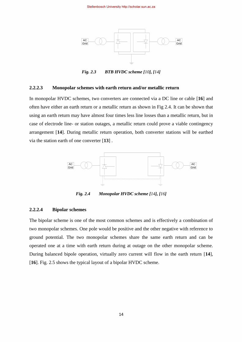
2.2.2.2 Back-to-back High Voltage Direct Current interconnection schemes
Back-to-back High Voltage Direct Current (BTB HVDC) interconnection schemes consist of
two converters connected back-to-back without any DC line as shown in Fig 2.3. These back-
to-back schemes are often used to interconnect between different AC grids where the power
flow needs to be controlled, to couple between AC grids with different frequencies or to de-
couple two AC networks dynamically from each other where existing dynamics problems
necessitate this [10], [11], [14], [23].
Stellenbosch University http://scholar.sun.ac.za
14
AC
Grid
AC
Grid
Fig. 2.3 BTB HVDC scheme [10], [14]
2.2.2.3 Monopolar schemes with earth return and/or metallic return
In monopolar HVDC schemes, two converters are connected via a DC line or cable [16] and
often have either an earth return or a metallic return as shown in Fig 2.4. It can be shown that
using an earth return may have almost four times less line losses than a metallic return, but in
case of electrode line- or station outages, a metallic return could prove a viable contingency
arrangement [14]. During metallic return operation, both converter stations will be earthed
via the station earth of one converter [13] .
AC
Grid
AC
Grid
Fig. 2.4 Monopolar HVDC scheme [14], [16]
2.2.2.4 Bipolar schemes
The bipolar scheme is one of the most common schemes and is effectively a combination of
two monopolar schemes. One pole would be positive and the other negative with reference to
ground potential. The two monopolar schemes share the same earth return and can be
operated one at a time with earth return during at outage on the other monopolar scheme.
During balanced bipole operation, virtually zero current will flow in the earth return [14],
[16]. Fig. 2.5 shows the typical layout of a bipolar HVDC scheme.
Stellenbosch University http://scholar.sun.ac.za

15
AC
Grid
AC
Grid
Fig. 2.5 Bipolar HVDC scheme [14], [16]
2.2.2.5 Multi-terminal Direct Current schemes
Multi-terminal Direct Current (MTDC) schemes can be described as a group of converters
connected to a common DC bus from where power can be imported or exported [14].
Coordination in terms of stable DC voltages, stable power and DC-side harmonics between
schemes is becoming more important with complex multi-terminal schemes [24]. One
possible MTDC layout is shown in Fig. 2.6.
AC
Grid
AC
Grid
AC
Grid
Fig. 2.6 MTDC scheme [14]
2.2.3 Other Voltage Source Converter technology and applications
Apart from VSC HVDC transmission schemes, other VSC Flexible AC Transmission System
(FACTS) devices also exist. These include the Static Synchronous Compensator
(STATCOM), Unified Power Flow Controller (UPFC) and the Static Synchronous Series
Compensator (SSSC) [11].
Although a VSC HVDC scheme is also effectively a STATCOM, the STACOM alone is used
in applications requiring rapid response to transient conditions, smooth voltage control over a
Stellenbosch University http://scholar.sun.ac.za

16
wide range of operating conditions and active harmonic filtering. Two such examples in the
United States are the VELCO Essex STATCOM rated at +133/-41 MVA at 115 kV and the
SDG&E Talega STATCOM iBTB rated at l00MVA with voltage level at 138 kV [11].
The UPFC consists of one series- and one parallel connected VSC with a common DC link
and energy storage using DC capacitors as shown in Fig. 2.7. This device can control both the
transmitted active- and reactive power, as well as the busbar voltage where the parallel
connected VSC is situated. The series element is effectively a SSSC and the parallel element
is effectively a STATCOM. Combined, these two elements give independent active and
reactive power flow over the connected line. The UPFC is functionally used for voltage
regulation, series compensation and phase shifting. The combinations of these functions
provide a very useful and versatile device for situations where high operating flexibility is
required [10], [11].
Line
SSSC
STATCOM
UPFC
Fig. 2.7 UPFC overview [10]
2.2.4 Current Source Converter technology and applications
Just as a VSC is a stiff DC voltage source provided by a DC capacitance, a Current Source
Converter (CSC), also known as a Current Source Inverter (CSI), is a stiff DC current source
provided by a DC inductance. A series-connected transistor and diode arrangement is used to
provide a bidirectional voltage blocking, unidirectional current conducting switch.
A common implementation of a current source converter is an Auto-Sequentially
Commutated Inverter (ASCI) device. Although the same fixed frequency modulation
strategies used in VSC applications can be used in CSCs and although CSC circuit
Stellenbosch University http://scholar.sun.ac.za

17
configurations have a lot of potential in high power drive systems, these advantages have not
been widely exploited to date [22].
2.2.5 Capacitor Commutated Converter HVDC configurations
Non-conventional HVDC circuit configurations such as the Capacitor Commutated Converter
(CCC) and Controlled Series Capacitor Converter (CSCC) have been proposed [25] with the
aim to provide improved immunity to commutation failure, lower load rejection over-
voltages and increased stability margins in power control mode. Although ferro-resonance is
a danger associated with CSCC configurations, this can be mitigated by controlling the
amount of series compensation.
2.3 Voltage Source Converter High Voltage Direct Current scheme composition
and main components
2.3.1 Overview of Voltage Source Converter High Voltage Direct Current scheme
composition
According to the CIGRE Protocol for reporting the operational performance of HVDC links
[26], the Institute for Electrical and Electronic Engineers (IEEE) Guide for the Evaluation of
the Reliability of HVDC Converter Stations [27] and partially by other sources [14], [16],
[28], [29], a complete interconnected HVDC scheme is generally divided into the following
main categories and sub-categories:
AC and auxiliary equipment:
AC filters and shunt banks
AC control and protection
Converter transformer
Synchronous compensator (not applicable to VSC schemes)
Auxiliary equipment and auxiliary power
Other AC switchyard equipment
Valves:
Valve electrical
Valve cooling
Valve capacitor
Stellenbosch University http://scholar.sun.ac.za
18
Phase reactor (added recently for VSC schemes)
DC Control and Protection:
Local control and protection
Master control and protection
Control and protection telecommunications
Primary DC equipment:
DC smoothing reactor
DC switching equipment
DC ground electrode
DC ground electrode line
DC filters
DC switchyard and valve hall equipment
DC Line
External AC network
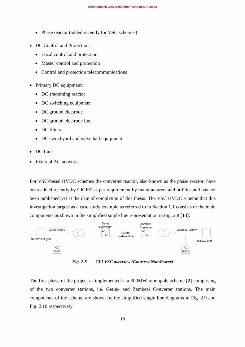
For VSC-based HVDC schemes the converter reactor, also known as the phase reactor, have
been added recently by CIGRE as per requirement by manufacturers and utilities and has not
been published yet at the date of completion of this thesis. The VSC HVDC scheme that this
investigation targets as a case study example as referred to in Section 1.1 consists of the main
components as shown in the simplified single line representation in Fig. 2.8 [13]:
AC
filters
AC
DC
DC
AC952km
overhead line
AC
filters
Zambezi 330kVGerus 400kV
Gerus
ConverterZambezi
Converter
NamPower gridZESCO grid
Fig. 2.8 CLI VSC overview (Courtesy NamPower)
The first phase of the project as implemented is a 300MW monopole scheme [2] comprising
of the two converter stations, i.e. Gerus- and Zambezi Converter stations. The main
components of the scheme are shown by the simplified single line diagrams in Fig. 2.9 and
Fig. 2.10 respectively.
Stellenbosch University http://scholar.sun.ac.za

19
HP60
filter
HP32
filter
HP3
filter
Converter
transformer
Converter
reactor
DC Smoothing
reactorDC Pole
breaker
Pole bus
-350kV
Neutral bus
400kV
225kV
Fig. 2.9 Gerus Converter station simplified single line diagram (Courtesy NamPower)
HP60
filter
HP32
filter
HP3
filter
Converter
transformer
Converter
reactor
DC Smoothing
reactorDC Pole
breaker
Pole bus
-350kV
Neutral bus
330kV
225kV
Fig. 2.10 Zambezi Converter station simplified single line diagram (Courtesy NamPower)
The CLI scheme that will be used for the case studies has the main circuit equipment and
functions detailed below. Some detail have been omitted to comply with confidentiality
clauses between the Utility and the Contractor.
2.3.2 Direct Current Pole Breaker and other primary Direct Current equipment
On the DC side of the converter station, there are various types of equipment like
links/disconnectors, high frequency filters, optical current transformers (OCTs) and surge
arrestors (detail not shown). The links/disconnectors allow for different operating
configurations such as metallic return and earth return, with parallel or single DC line
configurations in earth return configuration. The high frequency filters filter out switching-
frequency noise as well as accommodating the Power-Line Carrier (PLC) system. Surge
Stellenbosch University http://scholar.sun.ac.za

20
arrestors provide protection against switching and lightning impulses. The OCTs, Rogovski
coils and voltage dividers provide inputs to the protection and control system.
The Direct Current Pole Breaker (DCPB), consisting out of four separate units, is used during
DC line faults in conjunction with a auto-restart switching scheme in order to clear DC faults.
The word “breaker” is slightly misleading as a breaker cannot really break current. It is only
subsequent to a zero-crossing of a current waveform that opening mechanisms and arc
extinguishing methods can stop the current driven by strong inductive components in the
system from flowing. The same applies for a DC breaker. In order to break the current, a zero
crossing is created by commutating the DC current to a capacitor that resonates with the
series line inductance. This resonance gives opportunity for a zero crossing for the second
breaker to open. The third breaker opens a few milliseconds later in case the first zero
crossing is missed. The fourth breaker is used to bypass or switch in a damping resistor
during energising from the DC line side to limit converter transformer inrush currents [13].
2.3.3 Direct Current smoothing reactor
The DC smoothing reactor is used to limit transient over-currents during DC line faults and
also plays an important role in the DC side filtering design. The total harmonic content found
on the DC side of a 2-level VSC can be divided into DC and AC harmonics, or pole and
ground mode harmonics. DC harmonics modulated over from the AC side depend on the
relative fundamental current magnitude, modulation index and power factor.
AC-side zero sequence harmonics can be transferred via the mid-point connection and High-
Pass (HP60) filter to the DC side and are not cross-modulated. An ideal symmetrical system
will cause the DC-side harmonic content to contain both pole mode and ground mode
harmonics.
The smoothing reactor value is chosen such that it does not resonate with the DC line and
interconnected systems [13].
2.3.4 Insulated Gate Bipolar Transistor Valves
Each of the three phases from the AC system is connected to the midpoint of two IGBT
stacks (175kV DC). Each of the stacks contains a certain number of positions, of which a
certain percentage plus one position relates to the number of redundant positions and extra
margin to avoid tripping the converter. Each IGBT has a resistive and capacitive voltage
divider circuit that allows for even voltage distribution across all the IGBT‟s.
Stellenbosch University http://scholar.sun.ac.za
21
The IGBT positions for each valve are fired simultaneously either in Optimised Pulse Width
Modulation (OPWM) mode (under steady state conditions with cancellation techniques) at
23rd
harmonic, or normal PWM with third harmonic injection (under transient conditions
with high zero sequence content) mode at 33rd
harmonic [13].
2.3.5 Direct Current capacitors
The DC capacitors located between the pole- and midpoint buses and neutral bus to ground
have the purpose to store energy to help maintain a stable DC voltage, as well as to provide
fault level during AC faults [13].
2.3.6 Converter reactor
The converter reactor is a crucial piece of equipment in the AC/DC conversion process of the
converter stations. On the valve side of the converter reactor, the voltage waveform is that of
the PWM-switched DC voltage while on the AC side of the reactor the voltage waveform is
much closer to a fundamental component AC waveform at 225kV, but with a DC offset of -
175kV and several harmonic components. The converter reactor inductance with the
converter transformer gives the impedance required to control active and reactive power flow
[13].
2.3.7 Converter Transformer
The 300MVA 400/225kV or 330kV/225kV converter transformers connects the HVDC
scheme to the AC power system at the desired voltage level (in this case 330kV or 400kV)
and has a wide tap changer range in order to cater for different operating modes like reduced
DC voltage operation (in case of bush fires), black start conditions, etc. The transformer,
although built as three single phase transformers, has a star connection on the High Voltage
side and a delta connection on the converter (225kV) side. The delta connection does not
allow zero-sequence currents to flow into it [8] and simplifies external filter requirements.
The relatively high transformer impedance aids the converter reactor to obtain a bigger phase
angle change for active and reactive power control [13].
2.3.8 Converter Alternating Current breaker
The converter AC breaker connects the HVDC scheme to the AC grid and has the ability to
do several opening and closing operations in a short time in order to complete DC line fault
clearing sequences. The AC breaker also has a resistor with bypass breaker that is switched
during energising sequences in order to limit inrush currents into converter transformer, or to
Stellenbosch University http://scholar.sun.ac.za

22
limit inrush currents into the adjacent 315MVA coupling transformer during black start
operation [13].
2.3.9 Alternating Current filters
The scheme has three main AC filter banks, named according to their tuned frequencies,
namely HP60, HP32 and HP3. The HP60 filter connected between the converter reactor and
converter transformer has fairly flat impedance versus frequency response between the 55th
and 70th
harmonic order to filter our higher order harmonic distortion.
The HP32 filters are connected to the 330kV and 400kV AC busbars. This filter also has a
flat and damped response and caters for the 28th
to 35th
harmonic orders during OPWM
operation. It also targets the 33rd
harmonic order during PWM transient operation that would
normally occur only as a zero phase sequence harmonic, but would under unbalanced
conditions occur as positive- and negative phase sequence components on the HV side of the
converter transformer.
The HP3 filters are also connected to the 330kV or 400kV AC busbars. The HP3 filter at
Gerus converter station is tuned to 150Hz and caters for AC network 3rd
harmonic sensitivity
in that area. The HP3 filter at Zambezi is tuned to around 115Hz (closer to an HP2) and gives
a better response in terms of impedance magnification for the Zambian network. It will,
however, be shown that this tuning is not perfectly suited for transient and/or unbalanced
conditions [13].
2.3.10 Cooling and auxiliary equipment
The IGBT switching losses in the VSC scheme is significant and a pressurised water-cooled
system is used to transport heat away from the IGBT valves to be dissipated through cooling
fans outside the building. The AC and DC auxiliary systems include redundant medium
voltage (22kV) and low voltage (0.4kV) switchgear, diesel generator, battery banks (110VDC
and -50VDC), Uninterruptable Power Supply (UPS) systems and fire protection systems [13].
2.3.11 Protection and Control equipment
The protection and control equipment consists out of various cubicles where plant signals
terminate and are converted to protocol communications. Three individually redundant
control and protection systems monitor different areas of the scheme and communicate via
Ethernet communications networks with redundant network switches and interfaces. The
Stellenbosch University http://scholar.sun.ac.za

23
valve control and firing are controlled from one of these systems, but the lower level firing
pulses are done by individual and redundant valve control units.
Other equipment, such as line fault locators, power quality meters, tariff meters, fibre optic
terminal equipment (primary inter-station communications via Optical Pilot Ground Wire
(OPGW)) and PLC equipment (secondary inter-station communications), also form part of
the scheme. The OPGW line has 6 repeater stations and the PLC system has one repeater
station along the almost 1000 kilometres of line. Supervisory Control and Data Acquisition
(SCADA) data and engineering data is carried back to the control centre in Windhoek via
OPGW or digital PLC systems via Transmission Control Protocol / Internet Protocol
(TCP/IP) based protocols (IEC60870-5-104) with redundant routing options. The HVDC
scheme also interfaces with the AC substation automation systems that use the IEC61850
standard for publisher/subscriber information interchange. Aspects such as the practical
implementation of substation interlocking and bus zone protection via generic object
orientated substation event (GOOSE) messages will not be discussed as part of this thesis
[13].
2.4 Power system harmonic analysis overview
2.4.1 Fundamentals of power system harmonics
The generation of electricity by a utility is ideally required to be at a constant frequency, e.g.
50Hz or 60Hz, and to be purely sinusoidal. Even if this was the case, the sinusoidal voltage
that is applied to non-linear loads cause non-sinusoidal currents to flow through these devices
or loads. System impedances such as lines, transformers, etc between generation points and
loads can cause non-sinusoidal voltage drops, especially when non-sinusoidal load currents
are drawn. As a result, the voltage presented to load terminals also contains components that
contribute to the supply voltage not to be purely sinusoidal. Even linear loads presented with
non-sinusoidal voltages will then draw non-sinusoidal currents. These non-sinusoidal
components are considered QOS pollution and is referred to as power system harmonics
occurring as harmonic voltage- and harmonic current components [8], [12], [16], [22], [30],
[31], [32], [33], [34]. The term “harmonics” is a very broad term and is often misused. Proper
reference should be made using more descriptive and contextual terms such as “harmonic
component”, “harmonic distortion”, “harmonic order”, etc.
Stellenbosch University http://scholar.sun.ac.za

24
Power system harmonic components are theoretical constructs and are normally represented
as independently rotating phasors with rotational speeds of integer multiples of the
fundamental frequency rotational speed with a specific phase offset in relation to the
fundamental phasor. In a three-phase system harmonic components have certain phase-
rotation or sequence component characteristics. Harmonic components that do not rotate at
integer multiples of the fundamental frequency, called inter-harmonics, also exist in certain
cases and are often observed under transient conditions. Although this concept brings forth
some conflicting theoretical implications, it will not be discussed here [8], [12], [35], [36].
According to the work of Jean Baptiste Joseph Fourier (1768–1830) as first published in 1878
[37], any periodic waveform can be expanded in the form of a Fourier series as follows
[8], [12], [16], [22], [34], [38]:
where is the mean value of the periodic signal over one period given by the
relationship
The coefficients and are given by the relationships
and
where denotes the period of the waveform.
A simpler and more elegant form of the Fourier series is the complex exponential Fourier
series using the relationships
Stellenbosch University http://scholar.sun.ac.za

25
and
This gives
Let denote a complex coefficient related to and by the relationships
It follows that
where
The reason for using the complex exponential Fourier series and negative frequency
components are not only to provide a compact and more elegant mathematical description of
a periodic signal [38], but will later also help to give insight into the frequency domain
representation of the phase rotation of harmonic sequence components.
For discrete valued functions for numerical/computational purposes, the Discrete Fourier
Transform (DFT) or Fast Fourier Transform (FFT) is used. The discrete valued time domain
function is transformed into the frequency domain function of discrete
components given by the relationship [12]
where N is the number of samples per period.
Stellenbosch University http://scholar.sun.ac.za

26
The FFT is has a much more efficient computational algorithm and for large numbers of N a
significant computation time saving is achieved. The FFT takes advantage of the similarity of
many of the elements of the matrix formed by and by factorising this matrix of into
individual or factor matrices such that there are only two non-zero elements in each
row of these matrices, one of which is always unity [12], [38], [39].
2.4.2 Characteristic harmonic orders of power systems
Due to the symmetries found in power system wave shapes, the harmonics that normally
occur are referred to as characteristic harmonics. In general, the symmetry properties of the
wave shapes give rise to the following effects [8], [12], [16], [28], [38]:
Odd symmetry:
This results in al the terms cancelling out and the Fourier series containing only sine
terms.
Even symmetry:
This results in al the terms cancelling out and the Fourier series containing only cosine
terms.
Half-wave symmetry:
This results in a cancellation of all even order harmonics and a zero DC component.
In power systems, except where non-linearities cause half-wave symmetry to be
compromised, only odd harmonics are generated. Phenomena such as transformer saturation
by heavy loading or inrush currents can remove half-wave symmetry that introduces lower
order even harmonics [8], [12], [16], [28], [34], [40], [41].
2.4.3 Power system harmonic sequence components
In order to explain the harmonic interaction phenomena introduced by VSC schemes, it is
important to establish the concept of harmonic sequence components.
On a basis of inspection, [8] describes the individual harmonic components of balanced three
phase power systems to be entirely of positive-, negative-, or zero sequence by using the
Fourier representation of phase voltages:
Stellenbosch University http://scholar.sun.ac.za
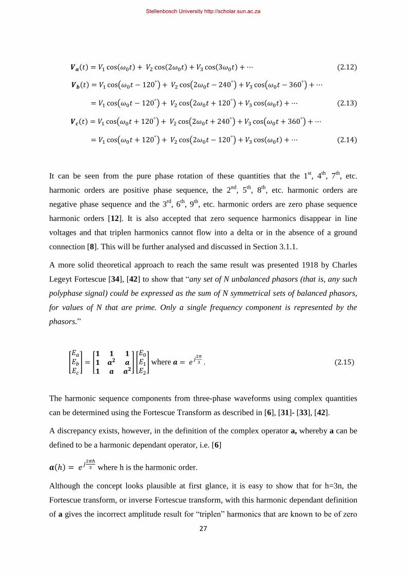
27
It can be seen from the pure phase rotation of these quantities that the 1st, 4
th, 7
th, etc.
harmonic orders are positive phase sequence, the 2nd
, 5th
, 8th
, etc. harmonic orders are
negative phase sequence and the 3rd
, 6th
, 9th
, etc. harmonic orders are zero phase sequence
harmonic orders [12]. It is also accepted that zero sequence harmonics disappear in line
voltages and that triplen harmonics cannot flow into a delta or in the absence of a ground
connection [8]. This will be further analysed and discussed in Section 3.1.1.
A more solid theoretical approach to reach the same result was presented 1918 by Charles
Legeyt Fortescue [34], [42] to show that “any set of N unbalanced phasors (that is, any such
polyphase signal) could be expressed as the sum of N symmetrical sets of balanced phasors,
for values of N that are prime. Only a single frequency component is represented by the
phasors.”
where
The harmonic sequence components from three-phase waveforms using complex quantities
can be determined using the Fortescue Transform as described in [6], [31]- [33], [42].
A discrepancy exists, however, in the definition of the complex operator a, whereby a can be
defined to be a harmonic dependant operator, i.e. [6]
where h is the harmonic order.
Although the concept looks plausible at first glance, it is easy to show that for h=3n, the
Fortescue transform, or inverse Fortescue transform, with this harmonic dependant definition
of a gives the incorrect amplitude result for “triplen” harmonics that are known to be of zero
Stellenbosch University http://scholar.sun.ac.za

28
sequence nature. For any harmonic component, it should be possible to express this harmonic
component in its positive phase sequence (PPS), negative phase sequence (NPS) and zero
phase sequence (ZPS) components, irrespective of its angular velocity. Relative phase angles
are harmonic order dependant, but are taken care of in the harmonic component expression
(3.1).
The non-harmonic dependant definition of
for a three-phase system is in fact valid
for determining the sequence components of waveforms containing harmonics [31]- [34] as
also acknowledged by Fortescue [42]. This is also confirmed by the complex number
theoretical expansion given in Section 3.1.1.
Harmonic sequence components can also be determined by using space vector components
represented by the Clarke‟s components [10], [41].
Another way to determine harmonic sequence components where real time calculation is
required, but without introducing the calculation delay typically experienced with discrete
time implementations [12], has been illustrated by connecting together a group of phase
locked loops in a special way in order to simultaneously separate out the sequence- and
harmonic components of waveforms typical in power systems [30]. A STATCOM was used
as a practical example to illustrate the robustness of this technique.
2.5 Principles of resonance and sensitivity
2.5.1 Conditions for resonance
For a true resonance condition to occur, two conditions need to be fulfilled, namely the
generation of a certain harmonic order and a sensitivity to that specific harmonic order due to
a series or parallel resonance point. The damping of the system will determine if the
resonance condition will remain damped or grow out of control while excited. The damping
is normally determined by the resistive components in the resonant circuit.
The movement of resonance points due to contingencies, system configurations, operating
regimes and the operating points of dynamic devices also plays an important role in the
harmonic analysis of a power system [6], [8], [12], [16], [34], [35].
Stellenbosch University http://scholar.sun.ac.za

29
2.5.2 Series resonance
A series resonance condition occurs in a series RLC circuit when the circuit impedance is at a
minimum when inductive and capacitive reactance cancels out each other. A small excitation
voltage then results in large currents [8], [12]. For a series RLC circuit, the total circuit
impedance is given by
where R is the resistance, the inductive reactance and the capacitive reactance of the
circuit.
It can be shown that is at a minimum when .
Using the relationship
where L is the inductance, the circuit frequency and using the relationship
where C is the capacitance, yields that is at a minimum when
The resonant frequency of the RLC circuit is thus given by
It can also be shown that the resonant harmonic is given by
2.5.3 Parallel resonance
A parallel resonance condition occurs in a parallel RLC circuit when the oscillating LC part
of the circuit is such that the inductive and capacitive reactances summate to zero and the
total parallel circuit impedance is at a maximum. A small excitation current thus results in
large voltage [8], [12]. For a parallel RLC circuit and using the relationships (2.17) and
(2.18), the total circuit impedance is given by
Stellenbosch University http://scholar.sun.ac.za

30
It can be shown that is at a maximum when .
Using the relationships from (2.17) and (2.18), it yields that is at a maximum when
The resonant frequency of the RLC circuit is thus given by
It can also be shown that the resonant harmonic is given by
2.5.4 System impedance versus frequency plots
In general for transmission systems, the positive phase sequence (PPS) impedance and
negative phase sequence (NPS) impedance is assumed to be very similar. However, in the
vicinity of large generation plant, the negative phase sequence can be slightly less due to the
fact that generator negative phase sequence impedance is less than positive phase sequence
impedance. The reason for this is that in the presence of NPS, the generator rotor sees a 2nd
harmonic rotating in an opposite direction to that of the fundamental PPS. This causes rotor
flux to saturate and lessens the flux penetration from the stator and thus yields a smaller
impedance value [16], [17].
Although system impedance versus frequency could be plotted for both the positive and
negative frequency domain due to different PPS and NPS system impedance, this is generally
not done for harmonic studies due to the small differences encountered [8], [17].
One representation of the frequency response of a transmission network is the system
impedance magnitude plotted against frequency to show parallel and series resonant points as
shown in Fig. 2.11. Accompanying this diagram should be another one showing the real and
Stellenbosch University http://scholar.sun.ac.za
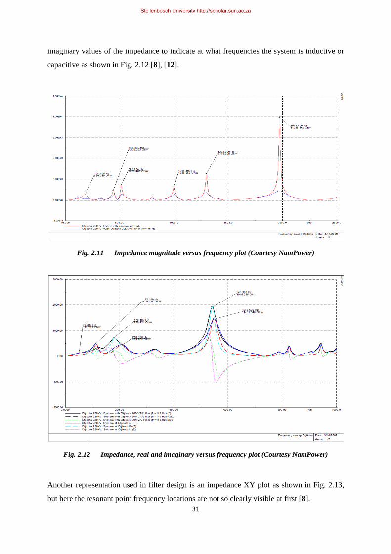
31
imaginary values of the impedance to indicate at what frequencies the system is inductive or
capacitive as shown in Fig. 2.12 [8], [12].
Fig. 2.11 Impedance magnitude versus frequency plot (Courtesy NamPower)
Fig. 2.12 Impedance, real and imaginary versus frequency plot (Courtesy NamPower)
Another representation used in filter design is an impedance XY plot as shown in Fig. 2.13,
but here the resonant point frequency locations are not so clearly visible at first [8].
Stellenbosch University http://scholar.sun.ac.za

32
Fig. 2.13 Impedance XY plot (Courtesy NamPower)
All series and parallel resonance points seen in an impedance plot are not necessarily
problematic. A rule of thumb for transmission systems to avoid dangerous resonance points is
to consider a window as shown in Fig. 2.14. This window includes the following area where
is the frequency, and is the system impedance at the nominal frequency of
50Hz. The window is defined by the relationship:
Stellenbosch University http://scholar.sun.ac.za

33
Fig. 2.14 Parallel and series resonant points [13]
For the harmonic integration of new equipment such as filter banks in the transmission
system, resonant points that move outside this area defined by the thumb rule combined with
the measured background harmonics normally give a good indication of probable resonance
problems [13]. (No clear published references for this rule of thumb could be found, except
for experiences from trusted filter bank designers.)
The reason for the typical system impedance increase of roughly
over the frequency
sweep is the dominance of inductive components in the transmission system, where
with h being the harmonic order [8].
2.5.5 Simplified system modelling and capacitor banks
Due to the characteristics of transmission system equipment i.e. a generator with series line
inductance and parallel capacitance, the system is considered to be predominantly inductive
at the nominal operating frequency. At frequencies above the first parallel resonance point
but below the next series resonant point, the system impedance could move to the capacitive
region. In this region, the system behaviour would change completely. Where a reactor
switched onto the system would normally lower the voltage, it would now raise the voltage.
Where a capacitor bank switched onto the system would normally raise the voltage, it would
now lower the voltage. For systems with very long transmission lines, low fault levels and at
Stellenbosch University http://scholar.sun.ac.za

34
high transmission voltages, the first parallel resonance point can move down very close to the
operating frequency. The danger of a 50Hz resonance condition becomes eminent and must
be properly managed [13].
When investigating the probable resonance point of a capacitor bank added to a system, an
approximate model can be used where the system is modelled only as a series resistance and
inductance. Adding a pure capacitor bank to the system then yield the following results [8]:
Using the relationships from (2.17) and (2.18), it yields that
and
The nominal frequency in Hz is related to the nominal angular velocity in radians per
second by
Using (2.26) and (2.27), let
For resonance to occur, . By substituting (2.28) and (2.29) into (2.23), the resonant
frequency is given by the relationship
Let the circuit inductive reactance be equal to the modelled system series reactance ,
and let the system short circuit power , be given by the relationship
where is the busbar voltage where the capacitor bank is connected.
The reactive power delivered by the capacitor bank is given by the relationship
Stellenbosch University http://scholar.sun.ac.za

35
Using (2.31) - (2.32) and substituting into (2.30) yields that
The resonant harmonic is therefore given by the relationship
As an example, according to the rule of thumb, a 40MVAR plain capacitor added to a system
with a fault level of 800MVA at any voltage level will resonate with the system at the
th harmonic. Should the fault level increase in future, the resonant point will
move towards the 5th harmonic and could pose problems should there be 5th harmonic
generation in the area.
To provide for system contingencies and future fault level and where only a reactive power
requirement is put forward and not to filter a specific harmonic order from the system,
damped C-type filters tuned to about 10Hz below the resonant harmonic are often used.
These filters are tuned such so as not participate directly in harmonic interactions and also to
cater for system frequency variations, but still to provide the required reactive power at 50Hz
[13].
Passive filter design for industrial applications using genetic algorithms to achieve the correct
Power Factor (PF) consisting of the Displacement Power Factor (DPF) and Distortion Factor
(DF) is an interesting recent development [43].
In cases where the placement of passive filters would cause too many complications with
either the creation of new resonance points or the movement of resonant points due to system
contingencies and fault level variations, either wide-band series/parallel filter solutions or
active filtering systems could be considered [44].
Stellenbosch University http://scholar.sun.ac.za

36
2.6 Voltage Source Converter theory overview
2.6.1 Forced commutated voltage source converters
The principle behind voltage source converters is the fact that a stiff DC voltage source
behind converted AC outputs gives voltage outputs instead of current outputs. Because the
commutation instants between valves are controllable and independent of the AC voltage, it
gives full control over the output of the converter. This is the principle of forced commutated
or self-commutated valve switching [10].
A common configuration for a three phase forced commutated converter VSC is the two level
bridge using IGBT valves with anti-parallel diodes as depicted in Fig. 2.15. Each bridge arm
can conduct current in both directions because of the uni-directionality offered by the diodes
and voltage polarity across each IGBT and diode switch combination. A change in power
flow direction can now be realised by changing the DC current direction. This is done by
changing the DC voltage of opposing converter stations allowing DC current to flow in the
desired direction. The stiff DC source is provided by the DC capacitors that can store a
significant amount of energy. Design considerations include active and reactive power
capability, harmonic injection limits, valve switching losses and cost implications [10], [22].
Udc/2
Udc/2
N g
Uva
Uvb
Uvc
Idc
Iva
Ivb
Ivc
Fig. 2.15 Basic VSC circuit layout [10]
2.6.2 Active and reactive power flow control
For any two interconnected AC power systems, the active and reactive power flow is
determined by the connecting impedance as well as the magnitude and angle between the two
Stellenbosch University http://scholar.sun.ac.za

37
voltage vectors [10], [16], [45]. In this case, the VSC scheme represents one voltage source
connected to an AC system via the combined converter reactor- and converter transformer
impedances as shown in Fig. 2.16 (also see Section 2.3.6 and Section 2.3.7):
UsysUVSC δ Xt
Ix
Fig. 2.16 Relative voltage angles and impedance (adopted from [10], [16])
The real power P that flows from the converter to the system is given by the relationship [10]
where is the system voltage, is the VSC terminal voltage, is the reactance
connecting the VSC to the system and denotes the voltage angle between the VSC and the
system. Similarly, the reactive power that will be exchanged between the VSC and the system
is given by the following relationship [10]:
From these equations it can be seen that for no voltage angle difference, the real power equals
zero and the reactive power is determined by the difference in voltage magnitudes. If
, Q is smaller than zero and implies inductive operation (VSC absorbs reactive
power). If , Q is larger than zero and implies capacitive operation (VSC delivers
reactive power to the system).
For equal voltage magnitudes, the reactive power equals zero and the real power is
determined by the voltage angle between the two vectors. If , power flows from the
VSC to the system (inverter operation) and if , power flows from the system to the
VSC (rectifier operation).
From the active and reactive power flow equations (2.35)-(2.36) it has been shown that four
quadrant power control is possible and although active and reactive power can be controlled
almost independently, there is a certain measure of coupling introduced by the VSC scheme
Stellenbosch University http://scholar.sun.ac.za

38
itself, as well as the connected AC systems. For reactive power control, the modulation index
controls the AC voltage magnitude and the reactive power flow and the firing instant of the
valves in relation to the AC side voltage determines the voltage phase angle and active power
flow. The power capability graph is limited by the AC current capability of the converter
(thermal limit) and the AC and DC voltage limits of the converter [10], [16].
For the voltages and currents shown in Fig. 2.17, the converter equations can be defined.
Ud
Uf UcUt
Id
Ir
If
It
Ul
Il
XrXtr
Zf
Fig. 2.17 VSC circuit quantities and flows (Courtesy ABB Sweden)
The converter voltage is given by the relationship
where is the AC filter bus voltage, is the converter reactor reactance and is the
current through the converter reactor.
The current is given by the relationship
where total current through the converter transformer and is the current through
the filter impedance .
The AC filter bus voltage is given by the relationship
Stellenbosch University http://scholar.sun.ac.za

39
where is the voltage on the primary side of the converter transformer connected to the
system and is the converter transformer reactance.
The filter current is given by the following relationship:
The converter equations as defined in (2.37) – (2.40) are shown as a vector diagram in Fig.
2.18.
It
If
Ir
UtUf
Uc
Xtr*ItXr*Ir
Φ
δ
Fig. 2.18 VSC circuit vector representation (Courtesy ABB Sweden)
In Fig. 2.18 Uc can be equated to the converter voltage ( ) and Ut to the system voltage
( ) without the transformer ratio and tap changer. Angle δ is the voltage angle across the
converter reactor and transformer impedances and angle Φ is the angle between output
voltage and current.
The illustration of a generator and infinite bus system with graph (generated by an Excel
model and equations) in Fig. 2.19 and Fig. 2.20 shows the change in active power flowing
between two systems as the voltage vector between them gradually increases due to a
difference running frequencies. During a power swing condition (see relevance to Section
2.1.2) the same applies [13].
Stellenbosch University http://scholar.sun.ac.za

40
Fig. 2.19 Generator connected to infinite bus (adopted from [16])
Fig. 2.20 Power swing of generator against infinite bus [13]
2.6.3 Insulated Gate Bipolar Transistor valve switching and operation principle
The operation principle of different VSC bridge configurations are generally the same and
commutation takes place between valves connected to the same phase. For a three phase AC
system, three sets of output voltages can be created at the desired frequency by switching the
correct IGBTs sequentially at the correct times. The direction of current through each bridge
arm is determined by which element, i.e. diode or IGBT, is conducting.
The basic relationships between AC and DC side quantities can be determined using the
equivalent circuit shown in Fig. 2.21 [10], [22].
Stellenbosch University http://scholar.sun.ac.za
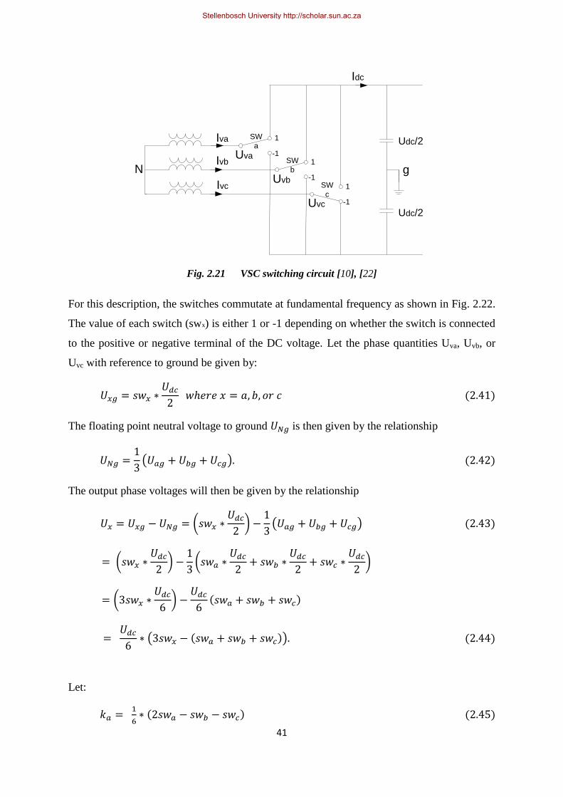
41
Udc/2
Udc/2
g
Uva
Uvb
Uvc
Idc
Iva
Ivb
Ivc
SW
a1
-1SW
b1
-1SW
c1
-1
N
Fig. 2.21 VSC switching circuit [10], [22]
For this description, the switches commutate at fundamental frequency as shown in Fig. 2.22.
The value of each switch (swx) is either 1 or -1 depending on whether the switch is connected
to the positive or negative terminal of the DC voltage. Let the phase quantities Uva, Uvb, or
Uvc with reference to ground be given by:
The floating point neutral voltage to ground is then given by the relationship
The output phase voltages will then be given by the relationship
Let:
Stellenbosch University http://scholar.sun.ac.za

42
and
This gives the phase quantities for the VSC in terms of the DC voltage and basic switching
functions [10], [22]:
The relationship between the switching positions and functions are shown in Fig. 2.22:
Stellenbosch University http://scholar.sun.ac.za

43
Fig. 2.22 VSC switching functions [10], [22]
Stellenbosch University http://scholar.sun.ac.za
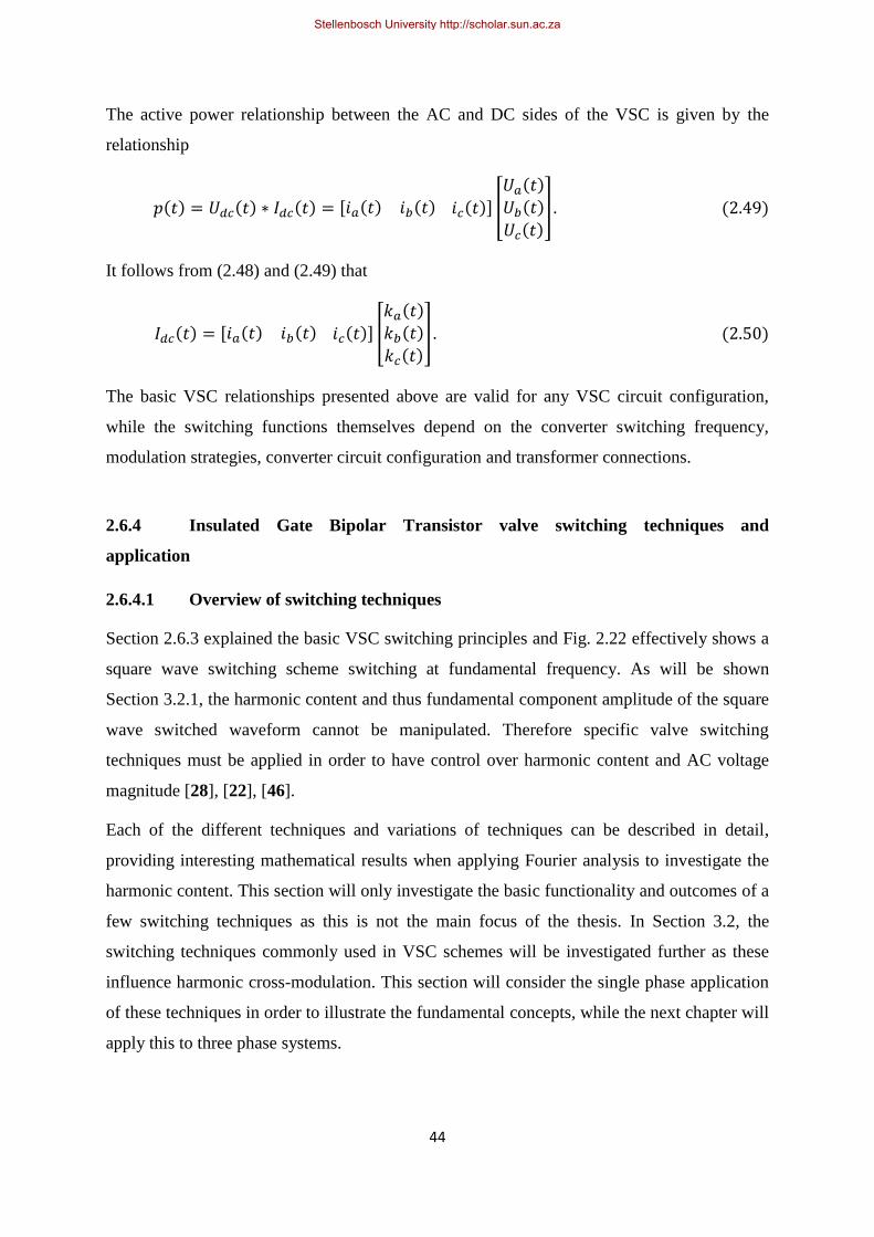
44
The active power relationship between the AC and DC sides of the VSC is given by the
relationship
It follows from (2.48) and (2.49) that
The basic VSC relationships presented above are valid for any VSC circuit configuration,
while the switching functions themselves depend on the converter switching frequency,
modulation strategies, converter circuit configuration and transformer connections.
2.6.4 Insulated Gate Bipolar Transistor valve switching techniques and
application
2.6.4.1 Overview of switching techniques
Section 2.6.3 explained the basic VSC switching principles and Fig. 2.22 effectively shows a
square wave switching scheme switching at fundamental frequency. As will be shown
Section 3.2.1, the harmonic content and thus fundamental component amplitude of the square
wave switched waveform cannot be manipulated. Therefore specific valve switching
techniques must be applied in order to have control over harmonic content and AC voltage
magnitude [28], [22], [46].
Each of the different techniques and variations of techniques can be described in detail,
providing interesting mathematical results when applying Fourier analysis to investigate the
harmonic content. This section will only investigate the basic functionality and outcomes of a
few switching techniques as this is not the main focus of the thesis. In Section 3.2, the
switching techniques commonly used in VSC schemes will be investigated further as these
influence harmonic cross-modulation. This section will consider the single phase application
of these techniques in order to illustrate the fundamental concepts, while the next chapter will
apply this to three phase systems.
Stellenbosch University http://scholar.sun.ac.za
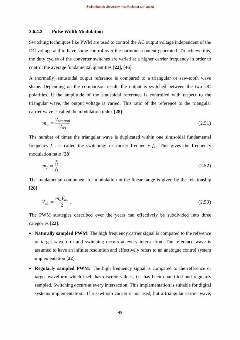
45
2.6.4.2 Pulse Width Modulation
Switching techniques like PWM are used to control the AC output voltage independent of the
DC voltage and to have some control over the harmonic content generated. To achieve this,
the duty cycles of the converter switches are varied at a higher carrier frequency in order to
control the average fundamental quantities [22], [46].
A (normally) sinusoidal output reference is compared to a triangular or saw-tooth wave
shape. Depending on the comparison result, the output is switched between the two DC
polarities. If the amplitude of the sinusoidal reference is controlled with respect to the
triangular wave, the output voltage is varied. This ratio of the reference to the triangular
carrier wave is called the modulation index [28]:
The number of times the triangular wave is duplicated within one sinusoidal fundamental
frequency , is called the switching- or carrier frequency . This gives the frequency
modulation ratio [28]
The fundamental component for modulation in the linear range is given by the relationship
[28]
The PWM strategies described over the years can effectively be subdivided into three
categories [22]:
Naturally sampled PWM: The high frequency carrier signal is compared to the reference
or target waveform and switching occurs at every intersection. The reference wave is
assumed to have an infinite resolution and effectively refers to an analogue control system
implementation [22].
Regularly sampled PWM: The high frequency signal is compared to the reference or
target waveform which itself has discrete values, i.e. has been quantified and regularly
sampled. Switching occurs at every intersection. This implementation is suitable for digital
systems implementation. If a sawtooth carrier it not used, but a triangular carrier wave,
Stellenbosch University http://scholar.sun.ac.za

46
sampling can be symmetrical or asymmetrical. Each of these choices has a slight effect on
the fundamental component as well as individual harmonic amplitudes [22].
Direct PWM: Also known as current-regulated modulation, switching occurs such that
the integrated output of the converter is equal to, or within a certain band of the integrated
target reference waveform. Two methods apply here, namely tolerance band control and
fixed frequency control [28].
A PWM technique to increase the maximum available modulation index and thus the
fundamental component magnitude applicable to three-phase inverters is called third-
harmonic reference injection. By using this technique, the modulation index can be increased
up to 1.15 by including a third harmonic injection of one-sixth without moving into the over-
modulation region. The third harmonic injection is a common mode injection and has no
effect on the phase to phase fundamental output voltage [22].
2.6.4.3 Square wave switching
Square wave switching is a special case of sinusoidal PWM where the modulation index
is so large that intersections between the carrier and reference waveform occur only when
the reference waveform reaches a zero-crossing (see Fig. 2.22). The fundamental component
is given by [22], [28]:
The frequency analysis of this switching scheme is continued in Section 3.2.1. The advantage
of this scheme is the low number of switching instants and thus lower losses for high power
applications. The drawback as stated in the introduction of this section is that the harmonic
content and fundamental component amplitude cannot be controlled.
2.6.4.4 Optimised/programmed Pulse Width Modulation
The principle behind OPWM or programmed harmonic elimination is that an output
waveform is constructed by switching at specific angles during the fundamental cycle. This
waveform is effectively a square-wave switching scheme that is combined with PWM in
order to typically control the fundamental component while minimising desired harmonic
components [22], [28].
Stellenbosch University http://scholar.sun.ac.za

47
The switching angles are determined by pre-determining for each desired modulation index
what the switching angles need to be to cancel out certain harmonics. If the modulation ratio
, then the number of angles available to switch at are
These angles are normally
numbered
. The equations that these angles have to fulfil simultaneously are
the formulas for the Fourier coefficients for the harmonic orders that are to be minimised, as
well as the fundamental component or modulation index determination [22], [28].
Solving these equations can be done my using an n-dimensional form of Newton‟s method,
or by using other non-linear solving algorithms provided by software packages such as
Matlab, Lingo64 and even Excel. Other methods have also been described by [47]. These
equations can be solved to control the fundamental- and harmonic components specifically,
to obtain certain performance characteristics according to a specification (eg. certain
allowable individual harmonic content or THD) or to minimise losses [22], [47], [48].
The maximum fundamental frequency component for this scheme is the same as for the
square-wave switching scheme and is given by [22], [28]:
2.6.4.5 Random Pulse Width Modulation
Where applications of PWM is required where spectral energy cannot be concentrated at
specific discrete frequencies, e.g. due to unwanted mechanical vibration in electrical
machines as a result of pulsating flux from current harmonics, one approach is to spread to
spectral energy over the frequency band and is referred to as Random Pulse Width
Modulation (RPWM). This must be achieved without substantially increasing harmonic
losses, considering band-limited noise generation and at the same time maintaining a linear
transfer function between the fundamental input and output of the scheme [22], [49].
To implement this, the period of the carrier frequency is randomly varied, while remaining
triangular within each half carrier period in order to maintain linearity of the modulation
process. In this way, the PWM duty cycle remains proportional over any single period of the
carrier signal to the value of the reference signal [22], [49].
Stellenbosch University http://scholar.sun.ac.za

48
2.6.4.6 Space Vector Modulation
Space Vector Modulation (SVM) is not a different modulation technique as such, but is a
method to view phase quantities in a different space/domain in order to make use of a
stationary plane as opposed to a rotating plane when doing online control [10]. (Also see
Appendix C). Using the Clarke and Park transforms, but with zero sequence components
included, the d-q-0 space vectors are used to represent the three phase quantities. For a three-
phase inverter, only eight possible switch positions are possible, of which two are short
circuit positions of the output. The remaining six positions represent active voltages as shown
in Fig. 2.22 and forms a rotating hexagon on the d-q plane for each switching instant [22].
Using the d-q-0 transformation gives the advantage that complex number calculations need
not to be done online by the control system and simplifies control strategy implementation
[10], [13].
2.7 Alternating Current / Direct Current systems interaction overview
2.7.1 Dynamic interactions
2.7.1.1 Overview of dynamic interactions
With regards to dynamic interaction between AC and DC systems, a complete study can be
dedicated to this topic. However, only a few concepts are highlighted here that have to be
taken into account in the designing, commissioning and operating HVDC schemes [4], [14],
[16]. Although similar, there are some subtle differences between the interactions observed
when considering classical HVDC schemes as opposed to modern VSC schemes:
2.7.1.2 Short-circuit ratio
Most AC/DC interactions (dynamic and harmonic) are strongly influenced by the AC system
strength compared to the HVDC scheme strength. This is often referred to as the system fault
level or system short-circuit ratio (SCR).
Although most sources refer to the classical HVDC converter MW rating, for VSC schemes
the MVA rating can also be used. A definition that includes the effects of AC-side equipment
such as filters, synchronous condenser, etc., is the Effective Short-Circuit Ratio (ESCR). The
Stellenbosch University http://scholar.sun.ac.za

49
ESCR classification is used traditionally to identify schemes in terms of potential interaction
problems [14], [16]. With reference to the ESCR, the risk for problems can be summarised as
follows:
ESCR > 3: High
2< ESCR<3: Low
ESCR<2: Very low
The ESCR of the Zambezi converter station is less than 0.7 under some network conditions
[13]. This indicates the significance of the references to the achievement of operating a VSC
scheme with overhead line on very weak AC systems [4].
The SCR or ESCR concepts have to be handled with caution as these definitions assume only
a fundamental component fault current contribution, as well a constant contribution over the
sub-transient and transient time windows. In reality, the fault current contribution changes
significantly during the first fundamental cycle in accordance with the network time constant
and DC capacitance discharge. Saturation effects and harmonic current contributions also
effects AC protection systems. As a result, protection coordination and discrimination based
on relay capabilities and reaction times become more complex. Modern relays that react
during the first quarter cycle may need to be set differently to relays that rely on a half or full
cycle buffered digital information [13], [16], [17].
2.7.1.3 Dynamic voltage interaction
During AC or DC system disturbances, the temporary blocking of the HVDC scheme could
cause significant overvoltages due to the AC filter equipment still connected to the possibly
weak AC systems. Depending on the fault clearing sequence, certain Transient Overvoltage
(TOV) equipment capabilities have to be observed, as well as regulatory QOS requirements.
Filter selection under weak network conditions can also be set differently to stronger network
conditions to alleviate extreme TOV conditions to some extent. The reactive power
requirements will also change during the blocked state due to the sudden change in active
power flow. For VSC schemes, active voltage regulation can only resume after de-blocking
again.
Another dynamic voltage problem can occur during high resistance DC line faults where the
AC systems supply the fault, but at a fault level less than the converter rated power
capability. During these conditions, the weak AC networks can suffer from severe voltage
Stellenbosch University http://scholar.sun.ac.za
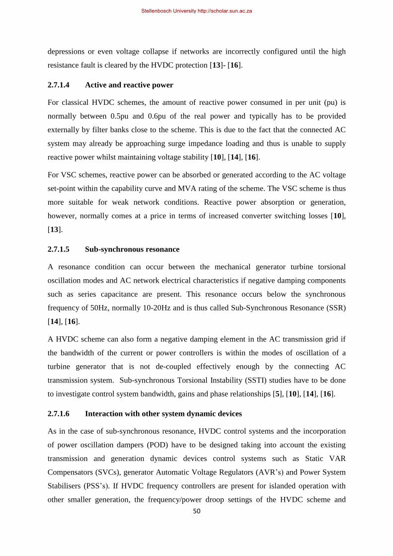
50
depressions or even voltage collapse if networks are incorrectly configured until the high
resistance fault is cleared by the HVDC protection [13]- [16].
2.7.1.4 Active and reactive power
For classical HVDC schemes, the amount of reactive power consumed in per unit (pu) is
normally between 0.5pu and 0.6pu of the real power and typically has to be provided
externally by filter banks close to the scheme. This is due to the fact that the connected AC
system may already be approaching surge impedance loading and thus is unable to supply
reactive power whilst maintaining voltage stability [10], [14], [16].
For VSC schemes, reactive power can be absorbed or generated according to the AC voltage
set-point within the capability curve and MVA rating of the scheme. The VSC scheme is thus
more suitable for weak network conditions. Reactive power absorption or generation,
however, normally comes at a price in terms of increased converter switching losses [10],
[13].
2.7.1.5 Sub-synchronous resonance
A resonance condition can occur between the mechanical generator turbine torsional
oscillation modes and AC network electrical characteristics if negative damping components
such as series capacitance are present. This resonance occurs below the synchronous
frequency of 50Hz, normally 10-20Hz and is thus called Sub-Synchronous Resonance (SSR)
[14], [16].
A HVDC scheme can also form a negative damping element in the AC transmission grid if
the bandwidth of the current or power controllers is within the modes of oscillation of a
turbine generator that is not de-coupled effectively enough by the connecting AC
transmission system. Sub-synchronous Torsional Instability (SSTI) studies have to be done
to investigate control system bandwidth, gains and phase relationships [5], [10], [14], [16].
2.7.1.6 Interaction with other system dynamic devices
As in the case of sub-synchronous resonance, HVDC control systems and the incorporation
of power oscillation dampers (POD) have to be designed taking into account the existing
transmission and generation dynamic devices control systems such as Static VAR
Compensators (SVCs), generator Automatic Voltage Regulators (AVR‟s) and Power System
Stabilisers (PSS‟s). If HVDC frequency controllers are present for islanded operation with
other smaller generation, the frequency/power droop settings of the HVDC scheme and
Stellenbosch University http://scholar.sun.ac.za
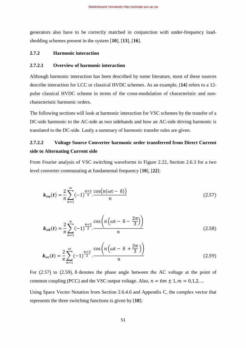
51
generators also have to be correctly matched in conjunction with under-frequency load-
shedding schemes present in the system [10], [13], [16].
2.7.2 Harmonic interaction
2.7.2.1 Overview of harmonic interaction
Although harmonic interaction has been described by some literature, most of these sources
describe interaction for LCC or classical HVDC schemes. As an example, [14] refers to a 12-
pulse classical HVDC scheme in terms of the cross-modulation of characteristic and non-
characteristic harmonic orders.
The following sections will look at harmonic interaction for VSC schemes by the transfer of a
DC-side harmonic to the AC-side as two sidebands and how an AC-side driving harmonic is
translated to the DC-side. Lastly a summary of harmonic transfer rules are given.
2.7.2.2 Voltage Source Converter harmonic order transferred from Direct Current
side to Alternating Current side
From Fourier analysis of VSC switching waveforms in Figure 2.22, Section 2.6.3 for a two
level converter commutating at fundamental frequency [10], [22]:
For (2.57) to (2.59), denotes the phase angle between the AC voltage at the point of
common coupling (PCC) and the VSC output voltage. Also,
Using Space Vector Notation from Section 2.6.4.6 and Appendix C, the complex vector that
represents the three switching functions is given by [10]:
Stellenbosch University http://scholar.sun.ac.za
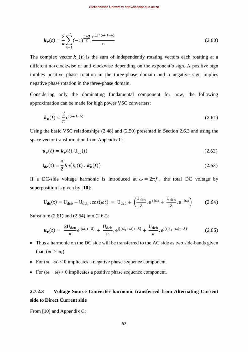
52
The complex vector is the sum of independently rotating vectors each rotating at a
different clockwise or anti-clockwise depending on the exponent‟s sign. A positive sign
implies positive phase rotation in the three-phase domain and a negative sign implies
negative phase rotation in the three-phase domain.
Considering only the dominating fundamental component for now, the following
approximation can be made for high power VSC converters:
Using the basic VSC relationships (2.48) and (2.50) presented in Section 2.6.3 and using the
space vector transformation from Appendix C:
If a DC-side voltage harmonic is introduced at , the total DC voltage by
superposition is given by [10]:
Substitute (2.61) and (2.64) into (2.62):
Thus a harmonic on the DC side will be transferred to the AC side as two side-bands given
that: (ω > ω1)
For (ω1- ω) < 0 implicates a negative phase sequence component.
For (ω1+ ω) > 0 implicates a positive phase sequence component.
2.7.2.3 Voltage Source Converter harmonic transferred from Alternating Current
side to Direct Current side
From [10] and Appendix C:
Stellenbosch University http://scholar.sun.ac.za

53
Substitute (2.61) and (2.66) into (2.63):
A positive sequence harmonic on the AC side transferred to the DC side gives only one of
the side-bands at (ωn- ω1).
A negative sequence harmonic on the AC side transferred to the DC side gives only one of
the side-bands at (ωn+ ω1).
An unbalanced harmonic on the AC side (with positive and negative phase sequence
components) will give two side-bands on the DC side [10]:
2.7.2.4 Alternating Current / Direct Current Harmonic transfer summary
The representation in Fig. 2.23 shows the summary of the AC/DC harmonic transfer rules as
derived above where the symbol (+) denotes PPS and (-) denotes NPS in the Space Vector
Domain:
Fig. 2.23 Harmonic transfer rules (adopted from [10])
Stellenbosch University http://scholar.sun.ac.za
54
Note that a single balanced three phase harmonic on the AC side only generates a single side
band on the DC and not both sides. Else, the wrong conclusion could be made that VSC
schemes do not only transfer harmonics between the AC to DC sides, but also proliferate the
number of harmonics infinitely [10].
2.8 Simulation techniques for electromagnetic transient- and harmonic studies
2.8.1 Transmission lines
The different mathematical models that exist to model transmission lines vary from the
simple T model and nominal or equivalent PI models with simple L and C parameters to
more complex and optionally distributed models where every physical attribute determining
the L and C components are taken into account. These range from the conductor bundling,
material conductivity, conductor spacing, tower geometry, ground resistivity, phase
transpositions, mutual couplings, etc. In general, the main parameters reduce to a series
resistance, series inductance, shunt capacitance and shunt conductance [8], [40].
Where multiple circuits on the same structure need to be taken into account, this geometry
must be indicated, as well as the parameters of line length and voltage level. Earth wire
spacing and conductor parameters are also important aspects [12], [40].
Typically a lumped or distributed model can be selected in software packages depending on
the intended simulation purpose. The increase in resistance and decrease in internal
inductance due to skin effect is proportional to √ω . For frequency sweeps above 1kHz and
for EMT- and harmonic distortion studies where long lines are present, a distributed model
with frequency dependant parameters, where both the surge impedance Zc and the
propagation factor are a function of the frequency, should be utilised for accurate results
[8], [12], [13], [50].
2.8.2 Power transformers
Transformer models in software packages are generally defined to include MVA rating,
positive- and zero sequence winding impedance in percentage and normally referred to the
HV MVA rating, copper losses, magnetizing impedance, zero-sequence magnetizing
impedance, tertiary winding parameters if a three winding transformer, vector group and
phase shift, neutral earthing parameters and tap changer parameters [40], [50], [51].
Stellenbosch University http://scholar.sun.ac.za

55
These parameters relate to the equivalent transformer circuit with an ideal voltage
transformation ratio, effective primary and secondary series resistances, primary and
secondary leakage reactances, shunt conductance that resembles iron losses and shunt
inductive susceptance that is equivalent to the quadrature magnetising current at no load [40],
[16], [50].
The transformer vector group, zero sequence circuit modelling and stray capacitances are
important to model correctly for EMT and harmonic studies. For studies of specific effects
such as transformer inrush currents and ferro-resonance [52], inter-winding stray
capacitances, winding to ground stray capacitances and core saturation should be included in
the transformer model. Saturation characteristics can normally be entered as a two-slope,
polynomial, or piece-wise linear approximation. Here the knee-point flux, linear
(unsaturated) reactance, saturated reactance and saturation exponent are common parameters.
Residual flux or remanence that plays a role in transformer energisation and inrush currents
and Ferro-resonance can also be modelled by specifying the d, q, 0 residual flux components.
Geomagnetically Induced Currents (GIC) can also be modelled by using the transformer
saturation parameters in conjunction with a DC voltage source in the transformer neutral
connection [50], [51].
2.8.3 Synchronous generators
Generators and motors are probably the most complex equipment to accurately model, with
many parameters applicable to different types of transient phenomena. These range from
synchronous, transient, to sub-transient and are important for protection- and EMT studies.
Important parameters are the direct axis synchronous reactance (Xd), direct axis transient
reactance (Xd‟), direct axis sub-transient reactance (Xd”), armature time constant (Td), direct
axis transient time constant (Td‟), direct axis sub-transient time constant (Td”), open circuit
voltage (E) and machine inertia constant (H) [40], [50].
Other machine stability parameters are the rotor saliency represented by the quadrature axis
parameters Xq, Xq‟ and Xq” and the associated time constants T‟qo and T”qo. The excitation
system modelling and governor system modelling depending on the prime mover type is also
important to model correctly for dynamic studies especially when considering machine
stability and the designing of power system stabilisers [16], [40].
With regards to harmonic studies, the machine sub-transient reactances and flux saturation
values are of importance. Harmonic content can cause increased copper and iron losses and
Stellenbosch University http://scholar.sun.ac.za

56
thus increased heat is a resultant effect. Pulsating torques is another effect that results due to
the interaction of harmonic-generated magnetic fields and fundamental frequency magnetic
fields. The rotor harmonics are also generated as a result of stator harmonics at one order less
than the stator harmonic order (hf-1) where the stator harmonic order is of positive or
negative phase rotation in the space vector domain. Harmonic orders of PPS and NPS pairs
can give rise to pulsating torques. For example, a combination of PPS harmonics (harmonic
orders of 4,7,10,...) and NPS harmonics (harmonic orders of 2,5,8,11) can give rise to
pulsating torques due to rotor harmonic orders of 3,6,9,12,... . Should the natural frequency of
the machine be close to one of these harmonic orders, super-synchronous resonance and
torsional oscillation leading to serious mechanical damage can occur [8].
2.8.4 Reactors, capacitors and filter banks
Reactors and capacitors are generally modelled simply as inductive (L) or capacitive (C)
components and in combination to form filter banks. The reactor series resistance (R) is also
modelled although normally relatively small. Filter bank configurations can range from a
simple series L and C combination, to a C-type filter with C1, C2, L and parallel R value, to a
double-tuned filter with series-parallel L and C combinations. In some packages, the filter
MVAR rating, tuning frequency and quality factor can be entered and the relevant L and C
values are automatically calculated. The three phase filter connection in star (where neutral
earthing details come into play) or delta with stray capacitances is also important for zero-
sequence circuit modelling [8], [40], [50].
2.8.5 Voltage Source Converter High Voltage Direct Current
For HVDC Voltage Source Converters, PWM switching elements and a PLL is normally
used in conjunction with DC capacitors, series reactor and or transformer, AC-side filters,
DC-side filters, DC line, etc. The complexity of the PWM element can vary from a steady-
state voltage source for loadflow simulations, to detailed firing control to simulate exact
valve firing in EMT studies. In order to protect the intellectual property of valve control
techniques, dynamic link library (DLL) files with valve control code are often compiled from
code to serve as a “black box” where manufacturer models are to be distributed to clients.
Several controllers are normally present to model the HVDC control system at each converter
station, namely DC voltage control, AC voltage or reactive power controllers, phase locked
loop to synchronise fire instants with AC system voltage and power control. Phase angle
measurement between the AC system and the valves across the converter reactor and
Stellenbosch University http://scholar.sun.ac.za

57
transformer is also required as an input to the active and reactive power controllers [14], [22],
[50], [51].
2.8.6 Harmonic loads
Normal loads can be modelled to be frequency dependent as either a series or parallel
combination of resistance and inductance whereby which these will draw different harmonic
currents due to harmonic voltages. This would be valid for harmonic load flows as well as for
EMT studies [8], [50].
For harmonic loads [53], the common practice is to specify harmonic currents as a percentage
of fundamental current in either balanced or unbalanced fashion. This can be used to model
for example a specific variable speed drive according to manufacturer data. A 6-pulse VSD
would for instance draw 5th
, 7th
, 11th
, 13th
, 17th
, 19th
... harmonics, while a 12-pulse VSD
would draw 11th
, 13th
, 23rd
, 25th
, etc. This method is normally only applicable to harmonic
loadflow studies. For EMT studies, harmonic EMT loads have to be modelled specifically for
certain software applications [8], [12], [50].
The hybrid time/frequency domain modelling of non-linear components proposed by B.C.
Smith et al [54] could also be used.
2.8.7 Dynamic models and simulation
Dynamic simulations are normally classified either as time domain root mean square (RMS)
or EMT simulations. The purpose of RMS studies are to observe the RMS values of
waveforms rather than instantaneous values and generally slower transient conditions where
slower control system phenomena such as generator AVR and governor behaviours, power
system stabilisers, sub-synchronous resonance due to series capacitors or control system
interactions, etc. need to be studied. Inter-machine and inter-area oscillation modes can be
better observed without the 50Hz component cluttering the waveform. The purpose of EMT
studies are to do small time step simulations in the microsecond range to observe
instantaneous values of waveforms to study electromagnetic transient effects during events
like equipment energisation, breaker pre-strike, fault conditions, harmonic- and resonance
phenomena, saturation, transferred saturation, ferro-resonance, travelling wave effects, TOV
and surge arrester studies [8], [13], [40], [16], [50], [51].
For dynamic studies, i.e. RMS or EMT, every dynamic device in the system would normally
have its control system modelled either as a piece of programmed code, a compilation of
Stellenbosch University http://scholar.sun.ac.za

58
logic functions, or a combination. These devices would include SVC‟s, HVDC schemes,
generator governor and AVR systems and automated reactor switching schemes.
The simulation time step size has a definite influence of the accuracy in some applications
like HVDC VSC schemes, but impacts negatively simulation execution time and requires
more processing power. This is where RTDS systems play an important role in factory testing
of systems as real-time simulations connected the actual plant protection and control system
hardware has a definite advantage. Yet, the quality of the output data is no better than a
normal computer using the same time step size and model to calculate the same output
results, although taking much longer to complete [13], [40], [50], [51].
2.8.8 Harmonic modelling and simulations
All equipment in the power system that has frequency dependant parameters must be
properly modelled in order to get accurate results when performing harmonic simulations.
The simplest harmonic simulation is a harmonic loadflow where essentially a normal
loadflow is performed at different frequencies and harmonic loads modelled to generate
harmonic voltages or currents with specified amplitudes and phase angles at specific
frequencies. In this way, pre-existing background harmonics that have been measured in the
field can also be modelled to get an accurate picture should new harmonic loads be added to
the system [55], [53].
For certain devices such as VSCs, an EMT model may be required to do time domain
simulations of the valve switching [56]. The EMT time domain waveforms from these
simulations then need to be analysed to determine the harmonic content in order to model an
accurate equivalent harmonic load. In most cases, the dynamics of the control system behind
the VSC element may perform such that a single harmonic load or PWM harmonic content
cannot be modelled and a harmonic loadflow study may prove insufficient. In this case,
frequency domain analyses of EMT waveforms are required to do a harmonic analysis [8],
[23], [35], [50], [51]. As referenced in Section 2.8.6, the hybrid time/frequency domain
modelling of non-linear components proposed by W. Wiechowski et al [54] could also be
used.
Stellenbosch University http://scholar.sun.ac.za

59
2.8.9 Frequency domain analysis
2.8.9.1 Simulation frequency sweep
The impedance versus frequency sweep simulation is done to ascertain the network frequency
response and to identify series and parallel resonance points. Although the impedance
magnitude is normally sufficient, the imaginary part of the impedance sometimes gives useful
information if the system will behave predominantly inductive or capacitive at a certain
frequency.
These frequency sweeps are useful in filter bank designs when adding a filter to an existing
network with known background harmonics. The network frequency response with and
without the filter under different contingencies can be compared to generate a harmonic
amplification curve to see what existing harmonics will be amplified and by how much. The
filter tuning frequency and quality factor can then be varied to obtain the best magnification
curve depending on the purpose of the filter. The magnification curves are to be compiled for
all different system contingencies and fault levels to ensure robust designs [8], [12], [40],
[50].
2.8.9.2 Fast Fourier Transformation – effects, limitations and alternatives
In practice, time domain waveforms that are generated by real life Transient Fault Records
(TFRs) or by time domain EMT simulations often have to be analysed to determine the
frequency domain information contained in it. For this, the most common transformation
used by modern computing systems is the Fast Fourier Transformation (FFT). However, this
sensitivity of the FFT to both the time resolution of the simulation and the periodicity of the
overall waveform has been highlighted. Where the small magnitude sideband or baseband
harmonics are of interest in harmonic analysis of PWM techniques using time simulation
studies, the FFT is only effective for exact integer carrier harmonic orders [22], [39].
According to the sampling theorem, the sampling frequency must at least be twice the highest
frequency contained in the original waveform to correctly transfer information to the sampled
system. The frequency component at half the sampling frequency is called the Nyquist
frequency. Misinterpretation of frequencies above the Nyquist frequency as lower
frequencies is called aliasing, but can be avoided by passing the original time domain signal
through a band-limited low pass filter with cut-off frequency set appropriately below the
Nyquist frequency [12], [38].
Stellenbosch University http://scholar.sun.ac.za

60
The windowing effect is inevitable as time domain functions can practically only be observed
for a limited time period with implied infinite periodicity. This effect can introduce errors in
the frequency spectrum as this effective multiplication by a rectangular window in the time
domain results in convolution in the frequency domain with a sinc pulse function. If the
window function is not synchronised to multiples of the fundamental frequency, non-periodic
noise will contribute to spectral leakage. This convolution in the frequency domain also gives
rise to the picket fence effect whereby the time domain function is effectively filtered by a
series of filters at integer multiples of 1/T where T is the sampling period. If the analysed
signal contains non-discrete, non-orthogonal frequencies, the non-ideal effect of the DFT
filter will cause such frequencies to be seen by more than one such time domain filter at a
time, but at reduced amplitude. This effect can be reduced by zero-padding. Adding a number
of zero values to the time domain waveform normally equal to the original record length
effectively increases the sampling period T by introducing extra DFT filters between the
original filters. Yet, the bandwidth of the original filters still depends on the original sampling
period and is not affected by zero-padding [12], [38], [57].
Alternatives to the FFT also exist, namely the Walsh transform, Hartley transform and the
Wavelet transform. If phase information is not required, the Hartley transform is an efficient
alternative to the FFT. The discrete implementation of the Wavelet Transform (DWT) is
normally implemented using Multi-Signal Decomposition (MSD) on different scales starting
at the Nyquist frequency downwards depending on the resolution required. High and low pass
filters are used to split each signal to the next scale level [12], [58]. The “fast non-similarity
wavelet transform” method has also been developed and describes techniques to decrease
computation time and to reduce storage space [59].
2.9 Simulation tools
2.9.1 General discussion on software simulation tools
In the power systems- and power electronics environment, there are many simulation
packages and tools available to assist the engineer in the modelling, simulation and analysis
of power systems including high-voltage devices that contain power electronics and control
systems. These tools also assist with the representation of data and interpretation of results.
The danger with any computerised simulation is that no mathematical model is a 100%
identical copy of reality and that any incorrect input parameter may give the wrong output
Stellenbosch University http://scholar.sun.ac.za

61
results. The principle of garbage in, garbage out applies. Certain modelling assumptions or
simplifications could also yield different results than measured in reality.
The other danger of computerised simulations is that of simply pressing a button and getting
results without doing some hand calculations to at least get an idea of what the results should
look like and just blindly accepting the simulation outputs. Results should make intuitive
sense and unexpected phenomena should be investigated and plausible reasons investigated
and tested.
Each simulation tool or package has certain strong points and certain weaknesses depending
on their intended purpose, developmental history, software platforms, operating systems, etc.
Each tool should be known and understood in order to select the right tool for the task
required. If two similar tools can do the same job, it could be worthwhile to compare results
and to try to identify and understand differences in results in order to make better choices for
future studies. License costs versus benefits also play a definite role, as well as after-sales
technical support, online support, etc. [8], [12], [13].
2.9.2 PSCAD/EMTDC
PSCAD/EMTDC is a power systems simulation tool that has been developed over many
years and started off in the 1970‟s as EMTDC (Electromagnetic transients and DC) as
inspired by Dr. Hermann Dommel‟s paper on Digital Computer Solution of Electromagnetic
Transients in Single- and Multiphase Networks [60]. The first version were utilised at
Manitoba Hydro on mainframe computers using punched cards and were used to analyse the
Nelson River HVDC power system in Manitoba, Canada. The first lines of code were written
Dennis Woodford at Manitoba Hydro who extended Dr Dommel‟s equations to HVDC
systems.
PSCAD is the graphical visual interface to EMTDC in which circuits are constructed,
simulations run and results plotted. Typical PSCAD studies include [51]:
Contingency studies of AC networks consisting of rotating machines, exciters,
governors, turbines, transformers, transmission lines, cables and loads
Relay coordination
Transformer saturation effects
Stellenbosch University http://scholar.sun.ac.za

62
Insulation coordination of transformers, breakers and arrestors
Impulse testing of transformers
Sub-synchronous resonance (SSR) studies of networks with machines, transmission lines
and HVDC systems
Evaluation of filter design and harmonic analysis
Control system design and coordination of FACTS and HVDC; including STATCOM,
VSC and cycloconverters
Optimal design of controller parameters
Investigation of new circuit and control concepts
Lightning strikes, faults or breaker operations
Steep front and fast front studies
Investigate the pulsing effects of diesel engines and wind turbines on electric networks
PSCAD/EMTDC is a very suitable tool and often the preferred tool for any EMT-related
study and therefore also for the analysis of HVDC schemes and harmonic interaction as
pertaining to the topic of this thesis, although the setting up of models and cases can take
some time and a certain amount of experience helps to correctly set up all the components.
With newer corporately endorsed 64-bit operating systems like Windows7, it may take some
time to correctly set up all the components and FORTRAN compiler. Initialisation of PSCAD
models and control systems has to be done in the correct manner to reach steady state values.
Then taking and storing snapshots with steady-state values to start the next simulation can be
done in order to save some time [13], [51].
2.9.3 DigSilent PowerFactory
Although DigSilent PowerFactory is perhaps a younger simulation tool, it caters for a wide
variety of studies, options and functions for different types of studies with an all-in-one
program, compiler, good models and a visual graphical user interface. Among the license
options that are selectable are:
Loadflow (Balanced or three-phase unbalanced)
Optimal power flow
Stellenbosch University http://scholar.sun.ac.za

63
Short circuit (complete, according to ANSI or according to IEC)
Stability functions (RMS, long term, EMT)
Flicker analysis
Contingency analysis
Reliability analysis
Generator adequacy analysis
Optimal Capacitor placement
Modal analysis
Network reduction (Loadflow, short circuit)
Harmonic calculation
Frequency sweep
Filter analysis
Distance Protection (Relay models)
Over-current protection (Relay models)
Other tools (DGS import and export)
State estimation
The building of networks, models and organisation of model parameters and data in the “Data
Manager” is simple and fairly intuitive. The setting up of cases, network variations,
initialisation of models, etc is also fairly simple to do. The 64-bit versions of PowerFactory
with multi-threading enabled runs a fair amount quicker than on a 32-bit system with single
processor.
The state estimation and RMS function have been used by NamPower as a real-time
simulator connected with the National Control Centre SCADA system to aid system
controllers in decision-making by providing a real time updated simulation environment from
system snapshots from where a certain operation can then be performed and the results
ascertained before performing the operation on the live system.
For protection-related studies, almost all modern protection relay models are available for
PowerFactory from the various relay manufacturers and can easily be used for protection
studies, settings calculations and other verification studies such as exporting a simulated
EMT file to a Comtrade format, importing into a waveform generator such as the Omicron
Stellenbosch University http://scholar.sun.ac.za

64
test set and injecting the voltages and currents into the real relay. Hereby true relay operation
can be compared with the relay model in PowerFactory [13], [50].
For the purpose of this thesis, the frequency sweep function and EMT stability functions
could be utilised. Loadflow simulations are almost always done as given and a quick check to
see that steady-state results make sense and that the model iterative methods with tolerances
solve without problems.
2.9.4 Real Time Digital Simulator systems
The purpose of Real time digital simulator (RTDS) systems is to incorporate specialised
software on a specialised hardware platform where small time step simulations need to be
executed in real time. As first developed at the Manitoba HVDC Research centre in the
1980‟s, RTDS Technologies (Inc) produced the world‟s first real time digital simulator.
RTDS systems have a wide area of application and are commonly use for the testing and
development of:
Protection and control schemes
Control systems of HVDC, SVC, synchronous machines and FACTS devices
AC and DC system operations and behaviour
Interaction of AC and DC systems
Demonstration and training purposes
The visual RTDS environment called RSCAD can run the same compiled code as generated
in PSCAD/EMTDC and is often used to switch between desktop studies and RTDS studies.
The hardware is based on a modular set up that includes parallel processing features,
input/output cards for interfacing to protection and control systems and different modes of
inter-card communication to avoid communications bottlenecks [13], [61].
RTDS systems have also been used in the NamPower network during the testing and
commissioning of the Auas SVC and Caprivi Link VSC HVDC schemes [13].
2.9.5 Matlab
The Matlab language of technical computing by Mathworks has been around since 1984 and
with its multi-domain simulation environment (Simulink) provides a powerful mathematical
tool to model anything from complex mathematical functions and algorithms to control
Stellenbosch University http://scholar.sun.ac.za

65
systems, signal processing, power systems, mechanical systems, financial modelling and
aeronautical systems, to automotive systems.
Although the application of Matlab is a lot wider than just power systems, many models do
exist for power systems components such as lines, transformers, synchronous machines,
voltage sources converters, etc.
Other useful functions that can be utilised in this thesis are its efficient FFT function and the
.m file programming function to execute sets of Matlab code. Interfacing between Matlab and
other simulation tools such as PSCAD, DigSilent PowerFactory, Excel, etc is also possible.
Matlab also supports OPC (Open Process Control) data links [13], [62].
2.9.6 MathCad
MathCad as owned by Parametric Technology Corporation was founded 1985 and is known
as an advanced engineering software package that allows the user to analyse/solve
mathematical or engineering problems while documenting it in a desired format [63].
MathCad has been widely used by power systems engineers in Southern Africa in the
calculating and documenting of relay protection settings, generator AVR and PSS design and
settings, reactor automation logic, etc. [13].
2.9.7 Excel
Although the use of the popular MS Office program Excel for engineering purposes is often
frowned upon by some engineers, it is a useful tool for the quick assessment of certain
electrical phenomena and to demonstrate certain principles although not simulating all
electrical parameters in detail [64].
Because of its complex number capability, Excel has been successfully used in filter bank
frequency responses, VSC AC/DC harmonic interaction, SVC external devices automated
switching schemes, generator governor response tests, SVC operating point harmonics
generation, harmonic sequence component analysis, high resolution FFT, transmission line
voltage sag, pole slip and power swing simulations, etc. [13].
In this thesis Excel has been used in AC/DC harmonic interaction, FFTs and solving of
OPWM simultaneous non-linear formulas.
Stellenbosch University http://scholar.sun.ac.za

66
2.9.8 Lingo64
Lingo64 by LINDO Systems Inc is an optimisation software package for linear, non-linear
and stochastic programming. Although the user interface is close to a text-based interface, it
is very efficient and very flexible [65].
In this thesis, Lingo64 has also been used in the solving of OPWM simultaneous non-linear
formulas to compare with Excel results.
Stellenbosch University http://scholar.sun.ac.za

67
3 Alternating Current and Direct Current harmonic interaction
3.1 Power system harmonic analysis
3.1.1 Harmonic sequence components
From Section 2.4.3 it was shown that the Fortescue transformation can be applied to non-
sinusoidal waveforms in a three phase system to calculate harmonic sequence components
and can thus be expanded as follows:
Let denote the harmonic voltage of phase k and of harmonic order h where h = 0,1,2,...:
According to (2.9), the total harmonic voltage will be given by the sum of the individual
harmonic components. The relative phase angles ( ) of the individual harmonic
phasors in relation to the fundamental component have been assumed to be zero for this
calculation in order to simplify:
A representation of the three phase voltages for each harmonic component for h=1, 2, 3
rotating at angular velocity is shown in Fig. 3.1:
Fig. 3.1 Harmonic component phase rotations
Stellenbosch University http://scholar.sun.ac.za

68
Manipulating (2.15), the sequence components of a three phase system are determined by:
, where n is the number of phases and k denotes the specific phase
(k=0,1,2,...,n-1).
It follows that:
for a three phase system to denote the reference phase (a) in this case.
for a three phase system to translate the b phase onto the reference (a)
phase.
for a three phase system to translate the c phase onto the reference (a) phase.
Also see [32], [42].
Assume a balanced system where .
The total ZPS voltage is then given by the following relationship and shows that ZPS
harmonic orders occur where h = 3n:
The total PPS voltage is given by the following relationship and shows that PPS
harmonic orders occur where h = 3n+1:
Stellenbosch University http://scholar.sun.ac.za

69
Lastly follows that the total NPS voltage is given by the following relationship and
shows that NPS harmonic orders occur where h = 3n+2:
This gives the information for Table 3.1 for the characteristic phase rotation of power system
harmonics under balanced conditions and is also confirmed by [8], [34]:
Table 3.1: Harmonic order phase rotations
ZPS PPS NPS ZPS PPS NPS
DC 1 2 33 34 35
3 4 5 36 37 38
6 7 8 39 40 41
9 10 11 42 43 44
12 13 14 45 46 47
Stellenbosch University http://scholar.sun.ac.za
70
15 16 17 48 49 50
18 19 20 51 52 53
21 22 23 54 55 56
24 25 26 57 58 59
27 28 29 60 61 62
30 31 32 63 64 65
It can also be shown that for phase-phase quantities, eg. , zero sequence components
disappear as given by the following relationship:
(Assume a balanced star-connected system where )
With a perfectly balanced system but with the presence of harmonics it can be seen that
positive, negative and zero sequence components can occur.
However, in a practical power system, there is always a measure of unbalance causing
harmonic orders that would characteristically occur for example as a ZPS harmonic, also to
contain PPS and NPS components.
For example, the zero sequence (3rd
, 9th
, ...) harmonic orders generated by Thyristor-Switched
Reactors (TCR‟s) in SVC‟s that are dependent on firing angle, normally circulate in the
strategically chosen TCR delta connections or delta winding of the SVC transformers [8].
Under unbalanced conditions, such as during single phase faults and reclosing cycles in the
system, TCR firing mismatch, inductor tolerances and unbalance in the system due to long
un-transposed lines or load imbalance, these harmonic orders would not circulate but escape
Stellenbosch University http://scholar.sun.ac.za
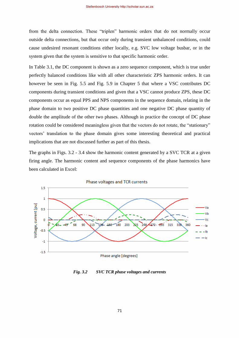
71
from the delta connection. These “triplen” harmonic orders that do not normally occur
outside delta connections, but that occur only during transient unbalanced conditions, could
cause undesired resonant conditions either locally, e.g. SVC low voltage busbar, or in the
system given that the system is sensitive to that specific harmonic order.
In Table 3.1, the DC component is shown as a zero sequence component, which is true under
perfectly balanced conditions like with all other characteristic ZPS harmonic orders. It can
however be seen in Fig. 5.5 and Fig. 5.9 in Chapter 5 that where a VSC contributes DC
components during transient conditions and given that a VSC cannot produce ZPS, these DC
components occur as equal PPS and NPS components in the sequence domain, relating in the
phase domain to two positive DC phase quantities and one negative DC phase quantity of
double the amplitude of the other two phases. Although in practice the concept of DC phase
rotation could be considered meaningless given that the vectors do not rotate, the “stationary”
vectors‟ translation to the phase domain gives some interesting theoretical and practical
implications that are not discussed further as part of this thesis.
The graphs in Figs. 3.2 - 3.4 show the harmonic content generated by a SVC TCR at a given
firing angle. The harmonic content and sequence components of the phase harmonics have
been calculated in Excel:
Fig. 3.2 SVC TCR phase voltages and currents
Stellenbosch University http://scholar.sun.ac.za

72
Fig. 3.3 SVC TCR phase currents harmonic content
Fig. 3.4 SVC TCR phase current harmonic sequence components
It can be seen that the TCR current harmonic sequence components calculated by using the
FFT and Fortescue transform follows the results in Table 3.1 as presented above, as well as
the characteristic odd harmonics described by Section 2.4.2.
The current harmonic content versus firing angle for a TCR generated in Excel is shown in
Fig 3.5. This illustrates why some resonant problems can be TCR operating point dependant
as mentioned in Section 2.5.1.
Stellenbosch University http://scholar.sun.ac.za

73
Fig. 3.5 SVC harmonic generation versus firing angle
3.1.2 Phase rotation in the frequency domain
When analysing a three phase system with or without the presence of harmonic components,
positive or negative phase rotation in the sequence domain can be observed and confirmed in
the frequency domain by doing a Fourier transform on the phase domain waveforms.
In the sequence domain, a phasor with positive phase rotation is given by:
In the sequence domain, a phasor with negative phase rotation is given by:
Using (2.15) in the phase domain and ignoring for this purpose, the reference phase “a”
would be given by the relationship
According to the complex exponential Fourier series in (2.9), the total harmonic voltage
signal, where h denotes the harmonic order, is given by the relationship
Stellenbosch University http://scholar.sun.ac.za

74
This gives rise to the following result
where in the phase domain is equal to the previously denoted in the sequence domain.
Thus a negative phase sequence component at any multiple of the fundamental frequency can
be regarded as a phasor with a negative frequency. This makes sense when considering the
result of Section 2.7.2.4.
This is also confirmed by the following example in Figs. 3.6 – 3.8 where an FFT is performed
on a waveform containing both positive and negative phase sequence components. The
resultant FFT in Fig.3.8 also shows the NPS component in the negative frequency domain
where , and is the resultant voltage phasors shown in Fig. 3.6:
Fig. 3.6 Positive and negative phase rotation in time domain
First the FFT of the real part of Ut is calculated and then the FFT of the imaginary part of Ut
is calculated resulting only in real valued frequency components. Recording the positive and
negative frequency domain quantities gives the results shown in Fig. 3.7 where the FFT of
the real part of Ut contains PPS and NPS components of 0.6 each. The FFT of the imaginary
part of Ut contains a PPS component of 0.4 and a NPS component of -0.4. Summating the
Stellenbosch University http://scholar.sun.ac.za

75
PPS and NPS components gives a total PPS component again of 1 and a NPS component of
0.2 .
Fig. 3.7 Frequency domain components of separate time domain components
To confirm the results, an FFT is done on the time domain total voltage Ut as shown in Fig.
3.8:
Fig. 3.8 Frequency components of summated time domain components
It can be seen that for , Ut will contain no imaginary component and equal PPS and
NPS components. The example above also confirms the well known identities of:
Stellenbosch University http://scholar.sun.ac.za
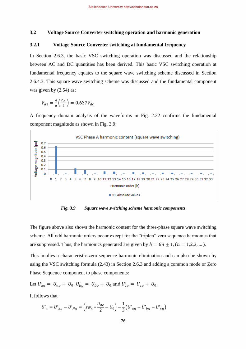
76
3.2 Voltage Source Converter switching operation and harmonic generation
3.2.1 Voltage Source Converter switching at fundamental frequency
In Section 2.6.3, the basic VSC switching operation was discussed and the relationship
between AC and DC quantities has been derived. This basic VSC switching operation at
fundamental frequency equates to the square wave switching scheme discussed in Section
2.6.4.3. This square wave switching scheme was discussed and the fundamental component
was given by (2.54) as:
A frequency domain analysis of the waveforms in Fig. 2.22 confirms the fundamental
component magnitude as shown in Fig. 3.9:
Fig. 3.9 Square wave switching scheme harmonic components
The figure above also shows the harmonic content for the three-phase square wave switching
scheme. All odd harmonic orders occur except for the “triplen” zero sequence harmonics that
are suppressed. Thus, the harmonics generated are given by .
This implies a characteristic zero sequence harmonic elimination and can also be shown by
using the VSC switching formula (2.43) in Section 2.6.3 and adding a common mode or Zero
Phase Sequence component to phase components:
Let ,
.
It follows that
Stellenbosch University http://scholar.sun.ac.za

77
The result above confirms that zero sequence components are not transferred or produced by
a VSC scheme. The only exception exists with configurations where zero sequence
components are transferred to the DC side via a midpoint filter coupling.
3.2.2 Pulse Width Modulation
As described in Section 2.6.4.2, switching techniques like PWM is used to be able to control
the AC output voltage independent of the DC voltage and to have some control over the
harmonic content generated. A sinusoidal output reference is compared to a triangular (or
saw-tooth) wave shape. Depending on the comparison result, the output is switched between
the two DC polarities. If the amplitude of the sinusoidal reference is controlled with respect
to the triangular wave, the output voltage is varied. This ratio of the reference to the
triangular wave is called the modulation index as given by (2.51):
The number of times the triangular wave is duplicated within one sinusoidal fundamental
frequency , is called the switching- or carrier frequency, . This gives the frequency
modulation ratio given by (2.52):
To recall, the fundamental component is given by (2.53):
The following example in Fig. 3.10 shows triangular PWM with and :
Stellenbosch University http://scholar.sun.ac.za

78
Fig. 3.10 PWM switching principle
Using the switching functions for ka, kb and kc given by (2.45) – (2.47) defined for VSC‟s
earlier in Section 2.6.3 gives the phase voltage wave shape as shown in Fig. 3.11 for phase A:
-1.5
-1
-0.5
0
0.5
1
1.5
0 45 90 135 180 225 270 315 360
Vo
ltag
e [p
u]
Phase angle [degrees]
Triangular Wave and Phase Reference Signals
Triangular Wave Phase A Phase B Phase C
-1.5
-1
-0.5
0
0.5
1
1.5
0 45 90 135 180 225 270 315
Vo
ltag
e [p
u]
Phase angle [degrees]
PWM Wave Phase A
PWM Phase A
Stellenbosch University http://scholar.sun.ac.za

79
Fig. 3.11 VSC switching phase quantity
Switching at higher frequencies eliminates the problem of sub-harmonics at
asynchronous PWM when the reference and triangular waves are not synchronised. This
technique moves harmonic content to higher frequencies, but increases the switching losses
and has a significant effect on high power applications. Triangular PWM produces harmonics
at
[28] as shown in Fig. 3.12:
Fig. 3.12 Triangular PWM switching harmonic content
-1
-0.5
0
0.5
1
0 45 90 135 180 225 270 315
Vo
ltag
e [p
u]
Phase angle [degrees]
Phase A Voltage from Triangular PWM
ka
0
0.2
0.4
0.6
0.8
1
0 11 22 33 44 55 66 77 88 99 Vo
ltag
e m
agn
itu
de
[pu
]
Harmonic order [h]
Triangular PWM harmonic content
ABS(FFT(PWM))
Stellenbosch University http://scholar.sun.ac.za
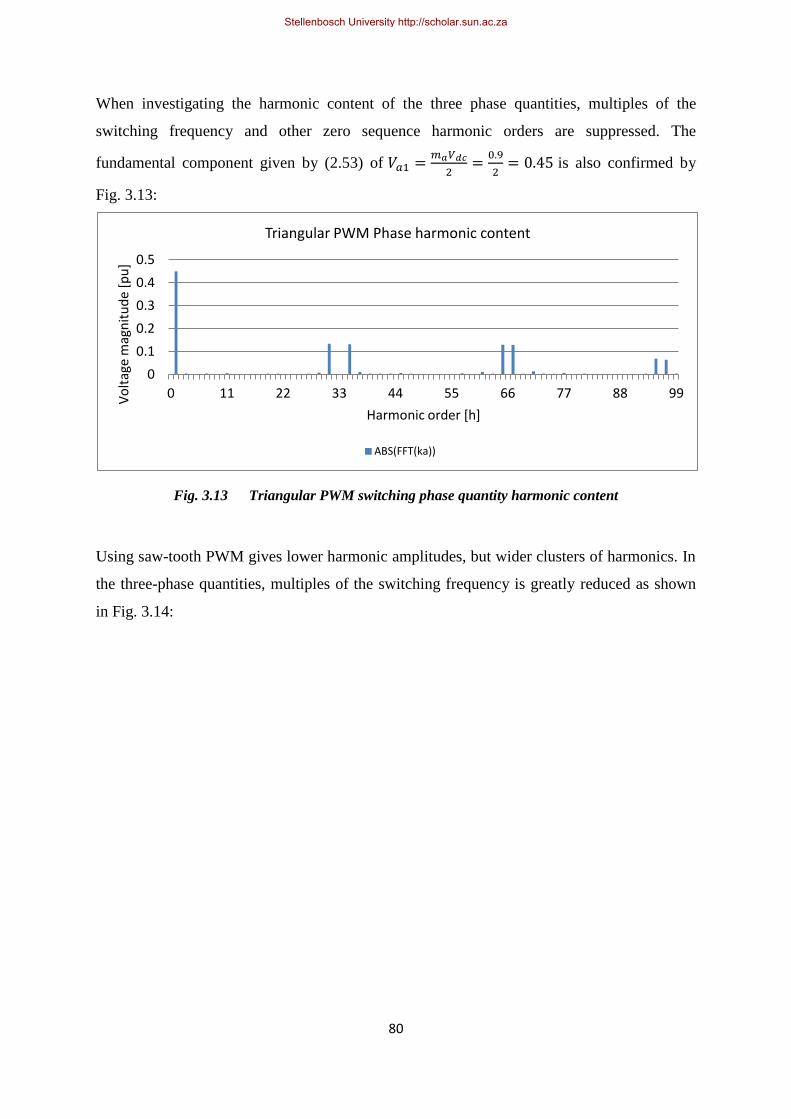
80
When investigating the harmonic content of the three phase quantities, multiples of the
switching frequency and other zero sequence harmonic orders are suppressed. The
fundamental component given by (2.53) of
is also confirmed by
Fig. 3.13:
Fig. 3.13 Triangular PWM switching phase quantity harmonic content
Using saw-tooth PWM gives lower harmonic amplitudes, but wider clusters of harmonics. In
the three-phase quantities, multiples of the switching frequency is greatly reduced as shown
in Fig. 3.14:
0
0.1
0.2
0.3
0.4
0.5
0 11 22 33 44 55 66 77 88 99 Vo
ltag
e m
agn
itu
de
[pu
]
Harmonic order [h]
Triangular PWM Phase harmonic content
ABS(FFT(ka))
Stellenbosch University http://scholar.sun.ac.za
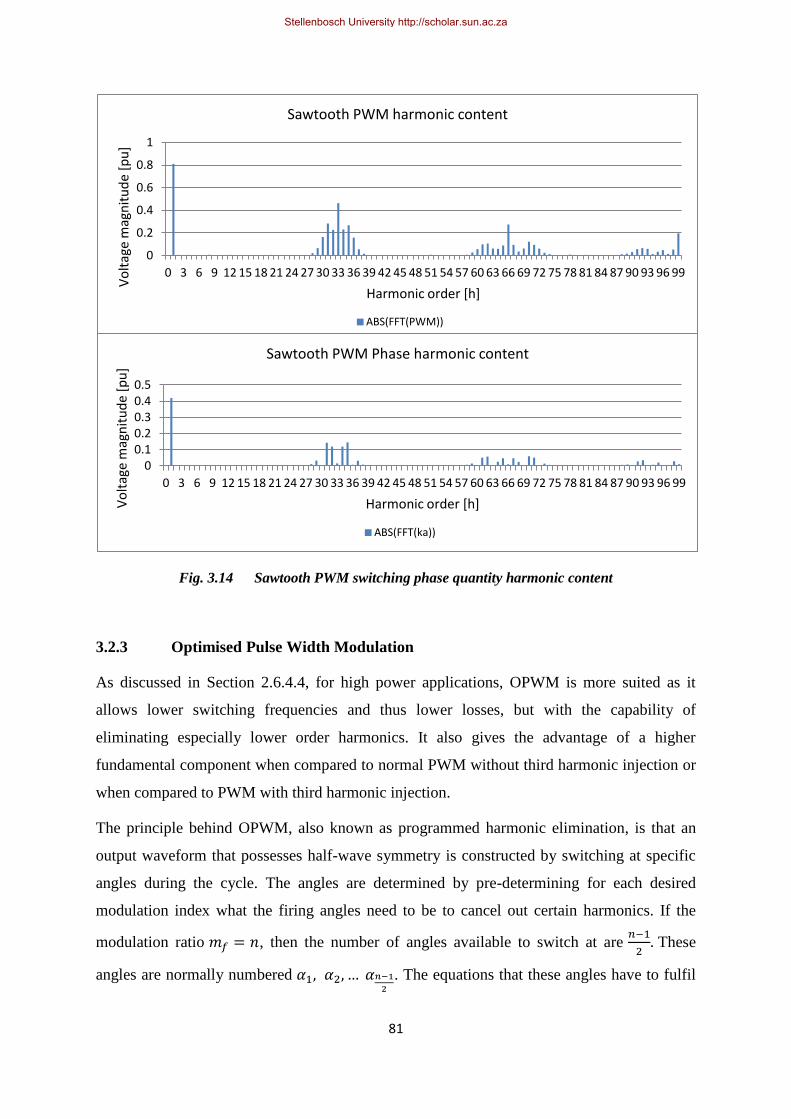
81
Fig. 3.14 Sawtooth PWM switching phase quantity harmonic content
3.2.3 Optimised Pulse Width Modulation
As discussed in Section 2.6.4.4, for high power applications, OPWM is more suited as it
allows lower switching frequencies and thus lower losses, but with the capability of
eliminating especially lower order harmonics. It also gives the advantage of a higher
fundamental component when compared to normal PWM without third harmonic injection or
when compared to PWM with third harmonic injection.
The principle behind OPWM, also known as programmed harmonic elimination, is that an
output waveform that possesses half-wave symmetry is constructed by switching at specific
angles during the cycle. The angles are determined by pre-determining for each desired
modulation index what the firing angles need to be to cancel out certain harmonics. If the
modulation ratio , then the number of angles available to switch at are
These
angles are normally numbered
. The equations that these angles have to fulfil
0
0.2
0.4
0.6
0.8
1
0 3 6 9 12 15 18 21 24 27 30 33 36 39 42 45 48 51 54 57 60 63 66 69 72 75 78 81 84 87 90 93 96 99
Vo
ltag
e m
agn
itu
de
[pu
]
Harmonic order [h]
Sawtooth PWM harmonic content
ABS(FFT(PWM))
0 0.1 0.2 0.3 0.4 0.5
0 3 6 9 12 15 18 21 24 27 30 33 36 39 42 45 48 51 54 57 60 63 66 69 72 75 78 81 84 87 90 93 96 99
Vo
ltag
e m
agn
itu
de
[pu
]
Harmonic order [h]
Sawtooth PWM Phase harmonic content
ABS(FFT(ka))
Stellenbosch University http://scholar.sun.ac.za

82
simultaneously are the formulas for the Fourier coefficients for the harmonic orders that are
to be minimised, as well as the fundamental component or modulation index determination.
For example, to switch at 9 times the fundamental frequency, 3 harmonic orders can be
eliminated and the modulation index can be set by solving the following equations
simultaneously:
To solve these equations, a non-linear solving program or iterative program has to be used.
Both the programs Lingo64 and Excel were used to obtain solutions to minimise lower order
harmonics. Below is an example of how to use Lingo64 to solve these equations:
MODEL:
! Find solutions for a1,a2,a3,a4;
[MOD1] 1 - 2*(@cos(a1)-@cos(a2)+@cos(a3)-@cos(a4)) > 0.939;
[MOD2] 1 - 2*(@cos(a1)-@cos(a2)+@cos(a3)-@cos(a4)) < 0.941;
[_5th] (1 - 2*(@cos(5*a1)-@cos(5*a2)+@cos(5*a3)-@cos(5*a4))) < 0.01;
[_7th] (1 - 2*(@cos(7*a1)-@cos(7*a2)+@cos(7*a3)-@cos(7*a4))) < 0.01;
[_11th] (1 - 2*(@cos(11*a1)-@cos(11*a2)+@cos(11*a3)-@cos(11*a4))) < 0.01;
! [_13th] (1 - 2*(@cos(13*a1)-@cos(13*a2)+@cos(13*a3)-@cos(13*a4))) < 0.01;
! [_15th] 1 - 2*(@cos(15*a1)-@cos(15*a2)+@cos(15*a3)-@cos(15*a4)) < 0.1;
! [_17th] 1 - 2*(@cos(17*a1)-@cos(17*a2)+@cos(17*a3)-@cos(17*a4)) < 0.1;
[total] min = @abs(1 - 2*(@cos(5*a1)-@cos(5*a2)+@cos(5*a3)-@cos(5*a4))
)+@abs(1 - 2*(@cos(7*a1)-@cos(7*a2)+@cos(7*a3)-@cos(7*a4)) )+@abs(1 -
2*(@cos(11*a1)-@cos(11*a2)+@cos(11*a3)-@cos(11*a4)))+@abs(1 -
2*(@cos(13*a1)-@cos(13*a2)+@cos(13*a3)-@cos(13*a4)))+@abs(1 -
2*(@cos(15*a1)-@cos(15*a2)+@cos(15*a3)-@cos(15*a4)))+@abs(1 -
2*(@cos(17*a1)-@cos(17*a2)+@cos(17*a3)-@cos(17*a4)) );
a1 < a2;
a2 < a3;
a3 < a4;
a4 < 1.570796;
END
After some experimentation and a lot of iterations, Excel seems to give better solutions when
evaluating the minimum sum of harmonics to be cancelled out. Below is an Excel example
with OPWM functions to minimise harmonic orders 5 to 17 while switching 9 times per cycle
Stellenbosch University http://scholar.sun.ac.za

83
depicted in Fig. 3.15. The four angles available when switching 9 times per cycle have been
determined at:
Fig. 3.15 OPWM switching and harmonic content
Investigating the three phase quantities and harmonic content, zero sequence harmonics also
disappear. The fundamental component is set by the equation determining the modulation
index to 0.94. Using (2.54), this gives the phase fundamental component of
which is the square-wave fundamental component times the governed
modulation index as shown in Fig. 3.16:
-1.5
-1
-0.5
0
0.5
1
1.5
0 23 45 68 90 113 135 158 180 203 225 248 270 293 315 338 360
Vo
ltag
e [p
u]
Phase angle [degrees]
OPWM Wave Phase A
OPWM Phase A
0
0.2
0.4
0.6
0.8
1
1.2
1.4
0 4 8 12 16 20 24 28 32 36 40 44 48 52 56 60 64 68 72 76 80 84 88 92 96 100
Vo
ltag
e m
agn
itu
de
[pu
]
Harmonic order [h]
OPWM Harmonic Content
ABS(FFT)
Stellenbosch University http://scholar.sun.ac.za

84
Fig. 3.16 OPWM switching and phase quantity harmonic content
To further investigate the influence that angle variations have on the harmonic content and
to get a better feeling of the simultaneous non-linear equations, a Matlab figure was created
by plotting the harmonic amplitudes for harmonic components 3,5,7,9,11,13 and 15 while
varying either of three angles between zero and 90 degrees. From this plot in Fig. 3.17 it
can be seen that a perfect cancellation solution does not exist, but only a “best-fit” solution
since the “valleys” or zero amplitude crossings do not fall in a perfectly straight line as the
harmonic order increases.
-1
-0.5
0
0.5
1
0 23 45 68 90 113 135 158 180 203 225 248 270 293 315 338
Vo
ltag
e [p
u]
Phase angle [degrees]
Phase A Voltage from OPWM
ka
0
0.1
0.2
0.3
0.4
0.5
0.6
0.7
0
4
8
12
16
20
24
28
32
36
40
44
48
52
56
60
64
68
72
76
80
84
88
92
96
10
0
Vo
ltag
e m
agn
itu
de
[pu
]
Harmonic order [h]
OPWM Phase Harmonic Content
ABS(FFT(ka))
Stellenbosch University http://scholar.sun.ac.za

85
Fig. 3.17 OPWM solution angle variations
Fig. 3.18 shows a plot from the actual Gerus converter station switching in OPWM mode at
1150Hz, i.e. 23 times per cycle. Thus the control strategy can cancel out 10 lower order
harmonics while maintaining the desired modulation index. The voltages and currents at PCC
are shown, as well as the filter bus voltage, valve currents and DC voltage. A frequency
analysis of the valve currents, as measured flowing through the valve before the midpoint
phase split-off, is shown in Fig. 3.19 and indicates high 3rd and 9th harmonic orders, as well
as a cluster of harmonics around the 32nd and 60th harmonic orders. When looking at the
phase currents at the PCC as shown in Fig. 3.20, zero sequence harmonics have been
suppressed as well as the cluster around the 60th harmonic by the HP60 filter. Only the 31st
harmonic component still exists that is filtered out by the HP32 filter on the 400 or 330kV
AC busbars.
Stellenbosch University http://scholar.sun.ac.za

86
Fig. 3.18 Gerus converter station steady-state waveforms
Stellenbosch University http://scholar.sun.ac.za

87
Fig. 3.19 Gerus converter station valve current harmonic content
Stellenbosch University http://scholar.sun.ac.za

88
Fig. 3.20 Gerus converter station current harmonics at PCC
Stellenbosch University http://scholar.sun.ac.za

89
3.3 Alternating Current / Direct Current Harmonic interaction theory
3.3.1 Harmonic amplitude transfer ratio
Apart from the AC/DC harmonic interaction theory presented in Section 2.7.2 that centres
primarily around harmonic cross-modulation and phase rotation, it would further be
interesting to observe the amplitude ratios with which harmonic components are transferred
between the AC and DC sides as this would help substantiate whether AC/DC harmonic
interaction is a phenomenon to be reckoned with, or if its effects could be considered
negligible.
One factor that would influence the harmonic amplitude transfer ratio (HATR) is the
harmonic transfer equations from Section 2.7.2 (2.65), (2.67) and (2.69). Another important
factor is the relationship to the relative fundamental component generation as determined by
the specific switching scheme. The specific PWM method (e.g. PWM or OPWM strategy),
modulation index, as well as other factors such as the external AC network frequency
response and DC-side frequency response could possibly influence the effective or measured
HATR from AC to DC or vice versa.
Another factor to consider is the simplification made in (2.61) whereby harmonic transfer is
only considered with regards to modulation by the fundamental component. The higher order
terms could also yield interesting results whereby introduced harmonics would also by
modulated by the switching scheme‟s characteristic or pre-existing harmonics.
3.3.1.1 Harmonic amplitude transfer ratio (HATR) from DC to AC side
From Section 2.7.2.2, the side band harmonics that will be generated from any DC harmonic
component has been derived, as well as their phase rotations.
From the same derivation in (2.65), the amplitude of the two AC side-band harmonics
can be seen for the basic VSC square wave switching operation where h indicates the DC
harmonic order:
Let the harmonic amplitude transfer ratio (HATR) be given by the relationship
Stellenbosch University http://scholar.sun.ac.za

90
This result yields that for a three-phase square-wave switching scheme and similarly for an
OPWM switching scheme:
The HATR for a three-phase PWM switching scheme can be derived by using the
relationship between the theoretical values for the fundamental components of a square wave
switching scheme and a PWM switching scheme.
As was given earlier by (2.54), the fundamental component for a square wave switching
scheme is given by:
The fundamental component for a PWM switching scheme is given by (2.53):
Using the relationship between (2.53) and (2.54) yields the following result:
To calculate the AC-side harmonic magnitudes, the basic VSC switching operation formula
multiplied by the fundamental component ratio above yields:
Substituting (3.22) into (3.19) yields that for a three-phase triangular-wave PWM switching
scheme:
In general, the two sidebands of the AC-side harmonics‟ amplitudes transferred from the DC
side will for any switching scheme be given by:
Stellenbosch University http://scholar.sun.ac.za

91
Section 4.3 uses the proposed HATR figures as derived above and tests these in different
simulation environments to establish their validity and applicability.
3.3.1.2 Harmonic amplitude transfer ratio from Alternating Current side to Direct
Current side
From Section 2.7.2.3, it can be seen that if any of the two AC sideband harmonics are
present, a single DC harmonic will be created with an amplitude ratio of:
This gives an effective AC to DC HATR of
and seems to be independent of the switching
technique or modulation index.
Section 4.3 uses the proposed HATR figure as derived above and tests this in different
simulation environments to establish their validity and applicability.
In practice, the AC voltage- and current harmonics presented to the VSC are related by the
system impedance at that specific frequency and transferred to the relevant DC-side
frequency depending on the AC-side harmonic phase rotation. Depending on the DC-side
frequency response and DC capacitor size, DC harmonics can be attenuated or filtered out.
The remaining DC-side harmonic is transferred back to the AC side depending on the scheme
specific HATR.
The effective cross-modulated voltage harmonics seen at the point of common coupling
(PCC) on the system-side of the converter reactor or converter transformer is strongly
influenced by the system impedance at those specific frequencies. Therefore low fault level
systems are much more prone to AC/DC harmonic interaction. In general, OPWM schemes
will show a larger total interaction transfer ratio than PWM switched schemes due to the
larger DC to AC HATR. The effect of third harmonic injection on PWM schemes‟ HATR has
not been investigated.
The diagram in Fig. 3.21 shows the AC-side and DC-side harmonics of a VSC scheme. A
13th harmonic PPS is introduced on the AC side and translates due to the fundamental
component to a (13-1)th or 12th harmonic on the DC side as two sidebands. The 12th
harmonic on the DC side translates back to an 11th harmonic NPS on the AC side.
Stellenbosch University http://scholar.sun.ac.za

92
Fig. 3.21 Harmonic transfer due to modulation by fundamental component
3.3.2 Modulation by scheme characteristic harmonics
The fundamental component of the VSC scheme is designed to be the largest and therefore
contributes the most to AC/DC harmonic interaction. Yet, it should be noted that the
characteristic or pre-existing harmonics of the scheme will also play a role although to a
lesser or even negligible extent.
If the simplification in (2.61) is not done, it can be shown that the higher order terms
depending on their amplitudes will modulate DC-side harmonics to new AC harmonics as
follows using (2.65). Instead of considering the fundamental component , each
characteristic harmonics that would normally be produced can be considered independently
as . This would yield:
This result shows that each DC-side harmonic will be transferred to the AC side at two
sidebands at radians apart from the DC harmonic. As shown as an example in Fig. 3.22, if
a scheme characteristically generates a relatively large 5th
harmonic NPS by design and a new
Stellenbosch University http://scholar.sun.ac.za

93
AC-side 13th
harmonic PPS is introduced, apart from the 12th
harmonic DC side component
and AC-side 11th
harmonic NPS harmonic produced by cross-modulation due to the
fundamental component, additional harmonics will be produced on the AC side at (12-5=7)
7th
harmonic as well as at (12+5=17) 17th
harmonic due to the 12th
harmonic DC component.
The phase rotation of the generated harmonics will depend on the phase rotation of the
generated characteristic 5th
harmonic. If the 5th
harmonic is characteristically with NPS, the
phase rotations will be opposite to those produced by the normal PPS fundamental
component.
The same 13th
harmonic (PPS) will also produce a smaller 18th
harmonic DC component due
to the generated NPS 5th
harmonic and cross-modulate to a relatively small 23rd
harmonic on
the AC side with NPS. If the 18th
harmonic DC component has any significant amplitude, it
will again modulate back to the AC side also with the fundamental component to a 19th
harmonic PPS and 17th
harmonic NPS. Depending on the existing 17th
harmonic, the new
superimposed value will depend on the relative phase angles of the two generated 17th
NPS
harmonics.
These statements are further demonstrated by simulation in Section 4.4 to provide more
clarity.
Fig. 3.22 Harmonic transfer due to modulation by scheme characteristic harmonics
Stellenbosch University http://scholar.sun.ac.za

94
4 Harmonic interaction simulation and modelling techniques
4.1 Modelling of NamPower and ZESCO transmission networks
Section 2.8 described the various modelling- and simulation techniques especially pertaining
to EMT- and harmonic studies. In order to study harmonic interaction phenomena, these
principles are important to obtain accurate results especially at higher frequencies.
For the complete NamPower network and southern ZESCO network, all transmission lines
with tower geometries and frequency dependant parameters, transformers, generators, filter
banks, SVC‟s and HVDC VSC have been modelled according to the principles described in
Section 2.8 so as to be valid both load flow-, harmonic load flow-, RMS dynamic-, EMT
dynamic studies and impedance versus frequency sweeps. The modelling of double circuit
lines in DigSilent PowerFactory however have the limitation that only a lumped line
parameter model can be selected as opposed to the preferred distributed model. Fortunately,
in the network vicinity where studies were conducted, no double circuit lines exist that would
influence the frequency response or EMT results. The Eskom network connected to the
Namibian network has been modelled as an external grid with appropriate fault level, X/R
ratio, inertia or acceleration time constant and secondary frequency bias in MW/Hz.
For EMT studies in DigSilent PowerFactory, a simplified HVDC VSC model excluding
certain controllers is used in order to simulate valve switching instants but does not replicate
the exact switching techniques employed in the PSCAD model, RTDS or real life scheme.
This model is valid and effective to illustrate the principles of AC/DC harmonic interaction,
but will not produce the exact same harmonic amplitude results as compared to the scheme‟s
recorded Transient Fault Records (TFRs) when attempting to reconstruct a real life harmonic
cross-modulation and resonance case.
Therefore, the case study example in Chapter 5 employs a DigSilent PowerFactory network
model that is accurate for impedance versus frequency sweeps, EMT study for line
energisation and time domain frequency analysis and checking of load flow results. A
PSCAD HVDC VSC model developed by the manufacturer of the HVDC scheme is used to
reconstruct the real life case study and confirm the preliminary PowerFacory results.
Stellenbosch University http://scholar.sun.ac.za

95
4.2 Development of Electromagnetic Transient mode harmonic voltage and current
sources
As the purpose of modelling the interconnected AC networks and HVDC VSC scheme is to
study AC/DC harmonic interaction, an essential component would be a harmonic voltage- or
current source to provide controlled AC-side generation of harmonic components of known
amplitude and phase rotation.
Although DigSilent PowerFactory has standard harmonic sources, these only operate in
harmonic load flows and not in RMS/EMT simulations. In order to simulate AC/DC
interaction, an EMT simulation is required to incorporate a detailed model for IGBT valve
firing. The problem is thus that harmonic sources would not be taken into account and
AC/DC harmonic interaction would not be visible in DigSilent PowerFactory simulations.
The solution was to create both harmonic voltage- and current sources by creating a
composite model that incorporates either the standard AC voltage source with two terminals
that can be put in series with the network to super-impose voltage harmonics, or the standard
AC current source with one terminal to be put in parallel with a busbar. The parallel-
connected harmonic current source effectively models a harmonic load that will translate to
voltage harmonics according to the system frequency dependant impedance. The standard
voltage source or current source components are then fed by a DigSilent simulation language
(DSL) script to output the desired harmonic content during EMT simulations at the desired
amplitudes and phase angles as governed by the chosen input parameters.
The first step is to create the library objects that will be referred to by the element objects. A
frame is created that houses the standard “Iac” or “Vac” element type, as well as a block
containing the DSL signal generator script. Although only creation of a harmonic current
source is shown, the process for the harmonic voltage source is similar. The two blocks are
connected by three signals that are named after the Iac or Vac internal variables designating
the phase currents or voltages as shown in Fig. 4.1:
Stellenbosch University http://scholar.sun.ac.za

96
Fig. 4.1 Harmonic current source library type
The second step is to create the DSL script that will feed the Iac or Vac element. The
“Signal_Gen” DSL element is set up with the correct parameters and internal variables and
the simple script is entered as shown in Fig. 4.2. The phase angle for each phase (Pha, Phb
and Phc) is defined as multiples of to make easy to enter a PPS (0, 4, 2) or NPS (0, 2, 4)
rotation as shown in Fig. 4.3.
Fig. 4.2 Harmonic current source DSL script
After the library objects have been created, the elements objects in the active grid can be
created and linked to the library items. The desired parameters defined in the DSL script can
be entered into the DSL parameter page shown in Fig. 4.3:
Stellenbosch University http://scholar.sun.ac.za

97
Fig. 4.3 Harmonic current source element type and frame
Fig. 4.4 shows the current- or voltage source outputs from the parameters entered in Fig 4.3.
The parameters yield an output waveform with the peak amplitude at 0.1kA, harmonic order
at 2 and the phase angle parameters yield negative phase rotation:
Fig. 4.4 Harmonic current source output of negative phase sequence, 2nd
harmonic
The result is a harmonic current or voltage source that is easily configurable and can now be
used in EMT simulations together with detailed VSC models to simulate AC/DC harmonic
interaction.
Stellenbosch University http://scholar.sun.ac.za
98
4.3 Harmonic Interaction models
4.3.1 Mathematical model in Excel
An Excel model has been built using the switching functions (2.45)-(2.47) derived in Section
2.6.3. The model incorporates the addition of a harmonic of specified order and magnitude to
be superimposed on the DC voltage. A FFT is done before and after the DC-side harmonic
activation and then a harmonic sequence analysis as is done on the three phase quantities to
confirm the phase rotation of the AC side harmonics. The results should confirm the
mathematical theory presented in Section 3.3.1.
The sampling rate is set at 2048 samples per cycle or 102.4kHz to eliminate some of the
unwanted effects of the FTT as discussed in Section 2.8.9.2.
First, a normal triangular PWM switching scheme at 33rd harmonic with modulation index
equal to 1 is presented in Fig. 4.5 and analysed.
Stellenbosch University http://scholar.sun.ac.za
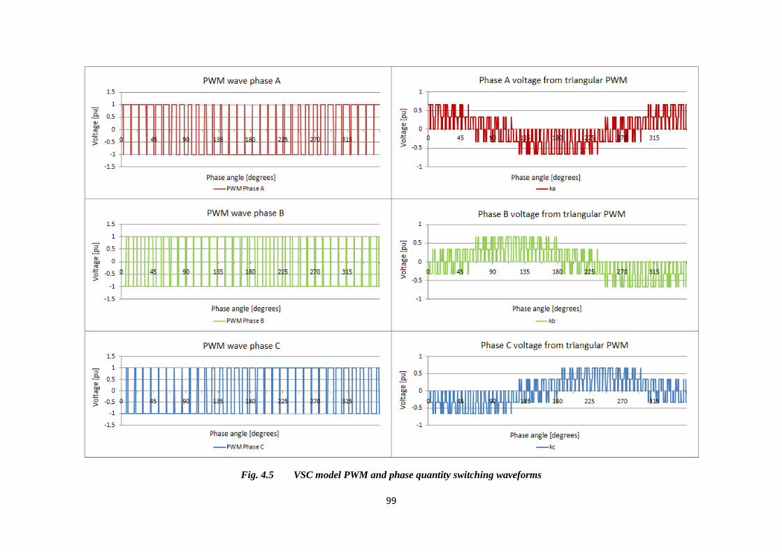
99
Fig. 4.5 VSC model PWM and phase quantity switching waveforms
Stellenbosch University http://scholar.sun.ac.za

100
The representation of the harmonic sequence components of the phase quantities in Fig. 4.5
for lower order harmonics is shown in Fig. 4.6. A relatively high switching frequency is
chosen not to have dominant lower order harmonics so that additional harmonic components
can easily be identified.
Fig. 4.6 Excel VSC model lower order harmonics
It is clear from Fig. 4.6 that no lower order harmonics of substantial magnitude are present
other than the fundamental component. Now a 6th harmonic is added to the DC voltage with
amplitude of 0.1 for demonstration purposes as shown in Fig. 4.7:
Stellenbosch University http://scholar.sun.ac.za

101
Fig. 4.7 Excel VSC model with 6th harmonic DC component
The 6th harmonic on the DC side is transferred to the AC side as a 5th harmonic with
negative phase sequence and a 7th harmonic with positive phase sequence. According to
(3.22) and (3.24) for a triangular PWM three-phase switching scheme, the transferred
harmonic amplitude would be:
= 2.5%
This agrees with the simulated values in Fig. 4.7.
The next example shows a 3rd harmonic on the DC side with the same amplitude of 0.1,
generating non-characteristic (even) harmonics on the AC side and also confirms the HATR
of the previous example. A 2nd harmonic with negative phase sequence and a 4th harmonic
with positive phase sequence is generated on the AC side with amplitude 0.025 or 2.5% as
expected as shown in Fig. 4.8:
Stellenbosch University http://scholar.sun.ac.za
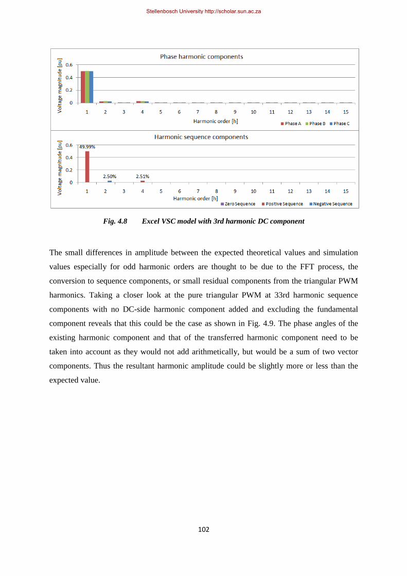
102
Fig. 4.8 Excel VSC model with 3rd harmonic DC component
The small differences in amplitude between the expected theoretical values and simulation
values especially for odd harmonic orders are thought to be due to the FFT process, the
conversion to sequence components, or small residual components from the triangular PWM
harmonics. Taking a closer look at the pure triangular PWM at 33rd harmonic sequence
components with no DC-side harmonic component added and excluding the fundamental
component reveals that this could be the case as shown in Fig. 4.9. The phase angles of the
existing harmonic component and that of the transferred harmonic component need to be
taken into account as they would not add arithmetically, but would be a sum of two vector
components. Thus the resultant harmonic amplitude could be slightly more or less than the
expected value.
Stellenbosch University http://scholar.sun.ac.za
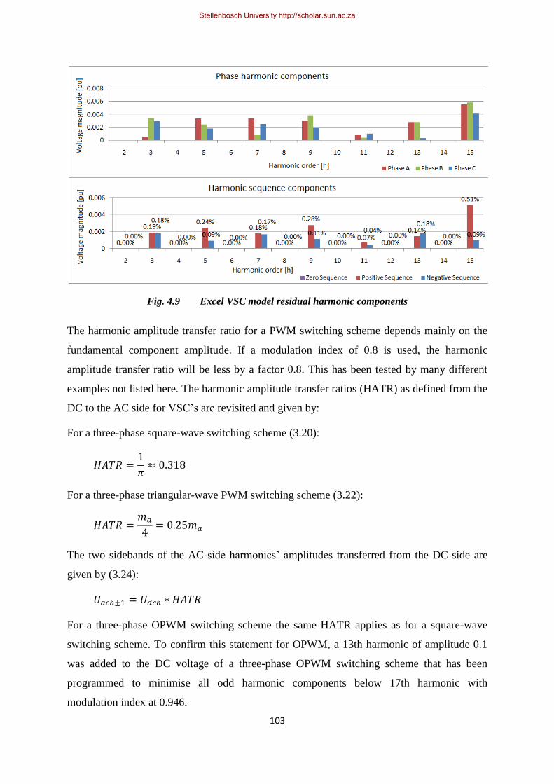
103
Fig. 4.9 Excel VSC model residual harmonic components
The harmonic amplitude transfer ratio for a PWM switching scheme depends mainly on the
fundamental component amplitude. If a modulation index of 0.8 is used, the harmonic
amplitude transfer ratio will be less by a factor 0.8. This has been tested by many different
examples not listed here. The harmonic amplitude transfer ratios (HATR) as defined from the
DC to the AC side for VSC‟s are revisited and given by:
For a three-phase square-wave switching scheme (3.20):
For a three-phase triangular-wave PWM switching scheme (3.22):
The two sidebands of the AC-side harmonics‟ amplitudes transferred from the DC side are
given by (3.24):
For a three-phase OPWM switching scheme the same HATR applies as for a square-wave
switching scheme. To confirm this statement for OPWM, a 13th harmonic of amplitude 0.1
was added to the DC voltage of a three-phase OPWM switching scheme that has been
programmed to minimise all odd harmonic components below 17th harmonic with
modulation index at 0.946.
Stellenbosch University http://scholar.sun.ac.za
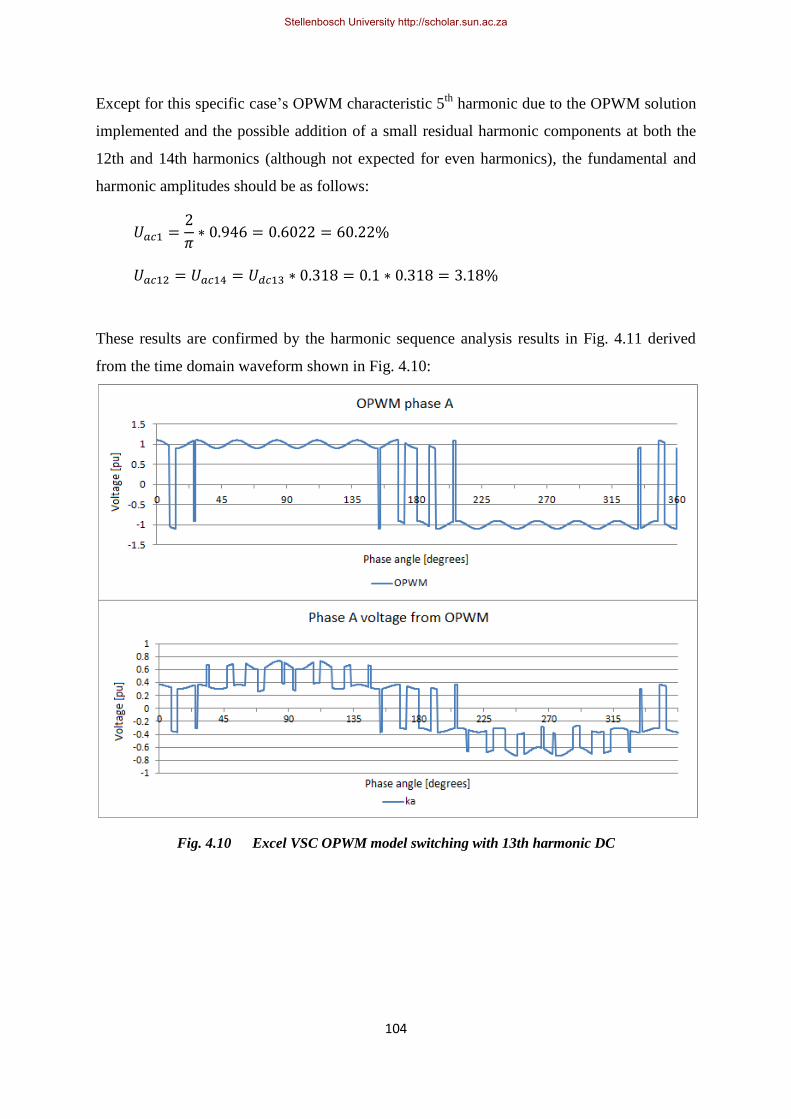
104
Except for this specific case‟s OPWM characteristic 5th
harmonic due to the OPWM solution
implemented and the possible addition of a small residual harmonic components at both the
12th and 14th harmonics (although not expected for even harmonics), the fundamental and
harmonic amplitudes should be as follows:
These results are confirmed by the harmonic sequence analysis results in Fig. 4.11 derived
from the time domain waveform shown in Fig. 4.10:
Fig. 4.10 Excel VSC OPWM model switching with 13th harmonic DC
Stellenbosch University http://scholar.sun.ac.za
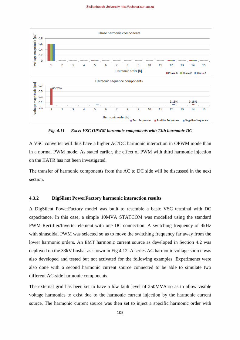
105
Fig. 4.11 Excel VSC OPWM harmonic components with 13th harmonic DC
A VSC converter will thus have a higher AC/DC harmonic interaction in OPWM mode than
in a normal PWM mode. As stated earlier, the effect of PWM with third harmonic injection
on the HATR has not been investigated.
The transfer of harmonic components from the AC to DC side will be discussed in the next
section.
4.3.2 DigSilent PowerFactory harmonic interaction results
A DigSilent PowerFactory model was built to resemble a basic VSC terminal with DC
capacitance. In this case, a simple 10MVA STATCOM was modelled using the standard
PWM Rectifier/Inverter element with one DC connection. A switching frequency of 4kHz
with sinusoidal PWM was selected so as to move the switching frequency far away from the
lower harmonic orders. An EMT harmonic current source as developed in Section 4.2 was
deployed on the 33kV busbar as shown in Fig 4.12. A series AC harmonic voltage source was
also developed and tested but not activated for the following examples. Experiments were
also done with a second harmonic current source connected to be able to simulate two
different AC-side harmonic components.
The external grid has been set to have a low fault level of 250MVA so as to allow visible
voltage harmonics to exist due to the harmonic current injection by the harmonic current
source. The harmonic current source was then set to inject a specific harmonic order with
Stellenbosch University http://scholar.sun.ac.za

106
either negative or positive phase sequence at suitable amplitude that would give a notable
harmonic voltage component of between 0.01pu and 0.1pu. Although it was tested, zero
phase sequence harmonic generation was not selected for an example because it is not
transmitted to the DC side of a VSC as proven earlier. The VSC control mode was set to
AC/DC voltage control and the voltage set-point was set to slightly above 1.1pu in order to
have the modulation index close to 0.75.
The time step and simulation output was set to 1µs and the FFT results were calculated using
4069 samples per period to retain good frequency resolution. Different sampled cycles in the
records was compared to ensure no differences occur.
To compare the simulation results with (2.67), the harmonic currents at the VSC terminals
and DC-side harmonic currents were measured. Because the STATCOM is connected to an
external grid, the grid‟s source impedance will influence the voltage harmonics as it would
provide an impedance path to sink the current harmonics flowing from the VSC. Therefore,
considering current harmonics should give a better view on the HATR. Fig. 4.12 shows the
single line diagram with load-flow results:
Stellenbosch University http://scholar.sun.ac.za

107
Fig. 4.12 PowerFactory STATCOM model single line diagram
4.3.2.2 Example 1:
The first example shown in Fig. 4.13 monitors the AC-side and DC-side harmonic
components when a 5th harmonic with positive phase sequence (non-characteristically) is
injected on the 33kV busbar:
E. Krige
PowerFactory 14.1.2
STATCOM model
Illustration of AC/DC harmonic interaction
Project: VSC ACDC
Graphic: Network Diagram
Date: 4/5/2012
Annex :
DC
-Bus
Bar
1.0
01
.00
0.0
0
0.4kV BB0.431.07
-30.00
33kV BB33.001.00-0.00
33kV PCC
33.001.000.00
~
AC Current Source..
-0.00 MW5.72 Mv ar
0.00
~
AC Current Source
-0.00 MW5.72 Mv ar
0.00
Ex ternal Grid
0.00 MW-7.18 Mv ar
0.00
STATCOM(1) 0.73
-0.00 MW20.00 Mv ar
-0.00
General L..
0.00 MW0.00 Mv ar
1.00
DC
-Cap
acita
nce
0.00 MW-7.18 Mv ar
0.00
-0.00 MW7.18 Mv ar
-0.00
LV
Trf
0.00 MW-18.61 Mv ar
0.00
-0.00 MW20.00 Mv ar
-0.00
DIg
SIL
EN
T
Stellenbosch University http://scholar.sun.ac.za
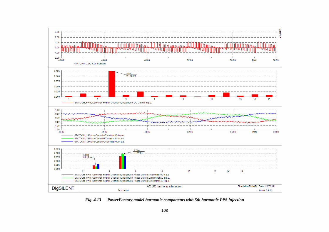
108
Fig. 4.13 PowerFactory model harmonic components with 5th harmonic PPS injection
Stellenbosch University http://scholar.sun.ac.za
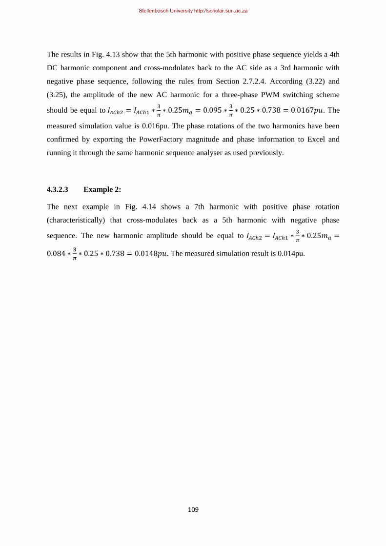
109
The results in Fig. 4.13 show that the 5th harmonic with positive phase sequence yields a 4th
DC harmonic component and cross-modulates back to the AC side as a 3rd harmonic with
negative phase sequence, following the rules from Section 2.7.2.4. According (3.22) and
(3.25), the amplitude of the new AC harmonic for a three-phase PWM switching scheme
should be equal to
. The
measured simulation value is 0.016pu. The phase rotations of the two harmonics have been
confirmed by exporting the PowerFactory magnitude and phase information to Excel and
running it through the same harmonic sequence analyser as used previously.
4.3.2.3 Example 2:
The next example in Fig. 4.14 shows a 7th harmonic with positive phase rotation
(characteristically) that cross-modulates back as a 5th harmonic with negative phase
sequence. The new harmonic amplitude should be equal to
. The measured simulation result is 0.014pu.
Stellenbosch University http://scholar.sun.ac.za

110
Fig. 4.14 PowerFactory model harmonic components with 7th harmonic PPS injection
Stellenbosch University http://scholar.sun.ac.za

111
Fig. 4.15 below confirms the expected harmonic sequence components as exported to the
Excel harmonic sequence component analyser:
Fig. 4.15 Harmonic sequence components with 7th harmonic PPS injection
4.3.2.4 Example 3:
The last example shows a 4th harmonic NPS injection that cross-modulates to a 6th harmonic
PPS. The new harmonic amplitude should be equal to
. The measured simulation result is 0.013pu. Compare this with
the PSCAD example in Section 4.3.3.1.
Stellenbosch University http://scholar.sun.ac.za

112
Fig. 4.16 PowerFactory model harmonic components with 4th harmonic NPS injection
60.0056.0052.0048.0044.0040.00 [ms]
3.00
2.00
1.00
0.00
-1.00
-2.00
STATCOM(1): DC-Current in p.u.
1 3 5 7 9 11 13 15[-]
0.25
0.20
0.15
0.10
0.05
0.00
STATCOM(1): Fourier-Coefficient, Magnitude, DC-Current in p.u.
5.000 0.111 p.u.
2 4 6 8 10 12 14[-]
0.10
0.08
0.06
0.04
0.02
-0.00
STATCOM(1): Fourier-Coefficient, Magnitude, Phase Current A/Terminal AC in p.u.
STATCOM(1): Fourier-Coefficient, Magnitude, Phase Current B/Terminal AC in p.u.
STATCOM(1): Fourier-Coefficient, Magnitude, Phase Current C/Terminal AC in p.u.
4.000 0.082 p.u.
6.000 0.013 p.u.
60.0056.0052.0048.0044.0040.00 [ms]
1.00
0.50
0.00
-0.50
-1.00
-1.50
STATCOM(1): Phase Current A/Terminal AC in p.u.
STATCOM(1): Phase Current B/Terminal AC in p.u.
STATCOM(1): Phase Current C/Terminal AC in p.u.
DIgSILENT AC / DC harmonic interaction Simulation Plots(2)
E. Krige
Date: 4/6/2012
Annex:
DIg
SIL
EN
T
Stellenbosch University http://scholar.sun.ac.za

113
The Excel harmonic sequence analysis confirms the 4th harmonic NPS and 6th harmonic PPS
phase rotations as shown in Fig. 4.17:
Fig. 4.17 Harmonic sequence components with 4th harmonic NPS injection
What was noted for other examples is that the cross-modulation amplitude factor seems to
decrease with higher harmonic orders and is attributed to the measured DC voltage harmonic
component decreasing as the injected frequency increases. The reason for this is thought to be
the DC-side frequency response of the STATCOM model where the impedance decreases
with because of the DC capacitance. This effect has not been noted in the Excel
examples as no DC-side filtering is modelled in Excel.
4.3.3 PSCAD interaction results
The PSCAD model used to test AC/DC harmonic interaction is the actual detailed model that
is also implemented in the CLI scheme and also the RTDS replica scheme. The time steps are
set to 4µs to have accurate IGBT valve switching instants. In the model, the VSC is supplied
via the DC line and connected to a passive network under light loading conditions where no
other fundamental frequency sources exist. Harmonic voltage sources are connected on the
AC-side of the VSC to each phase via the two 315MVA coupling transformer impedances at
220kV on the passive network side.
4.3.3.1 Example 1:
For this example, a 4th harmonic with negative phase sequence is injected under steady state
conditions after 1 second and the time domain waveforms were analysed to determine the
cross-modulation factors. The modulation index of the converter was measured at 0.78. The
PSCAD results were exported to a Comtrade format and the Matlab program written as is
Stellenbosch University http://scholar.sun.ac.za
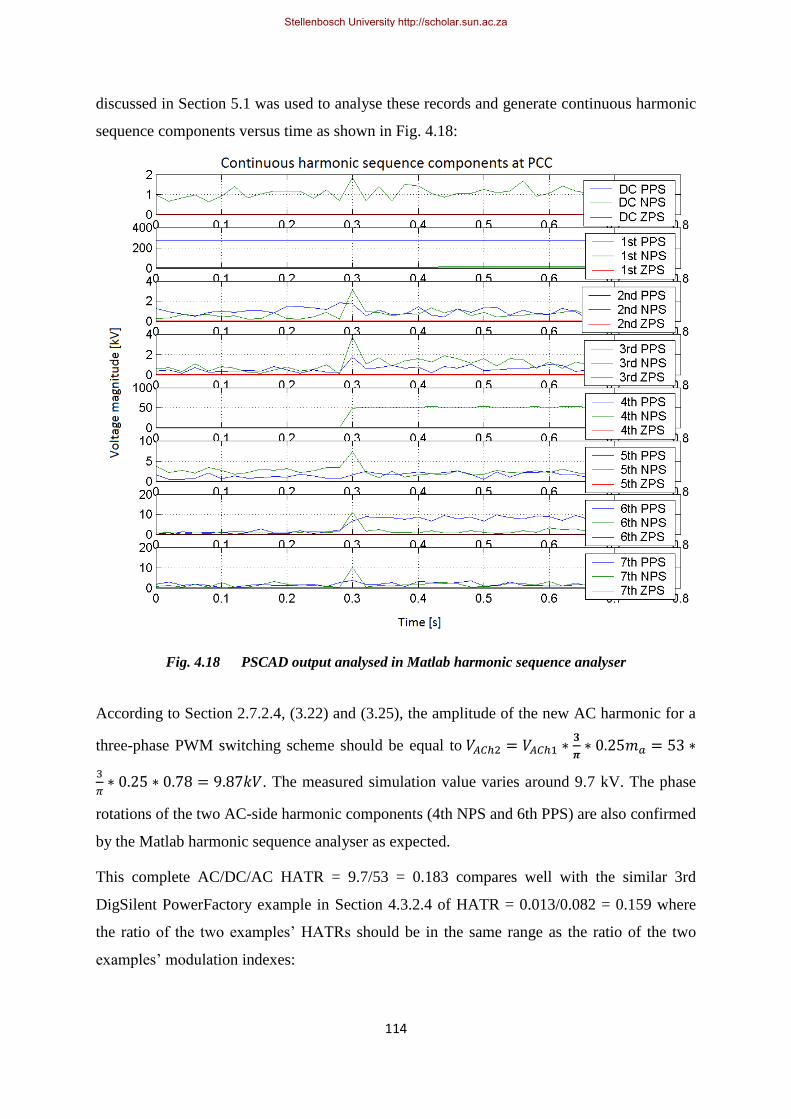
114
discussed in Section 5.1 was used to analyse these records and generate continuous harmonic
sequence components versus time as shown in Fig. 4.18:
Fig. 4.18 PSCAD output analysed in Matlab harmonic sequence analyser
According to Section 2.7.2.4, (3.22) and (3.25), the amplitude of the new AC harmonic for a
three-phase PWM switching scheme should be equal to
. The measured simulation value varies around 9.7 kV. The phase
rotations of the two AC-side harmonic components (4th NPS and 6th PPS) are also confirmed
by the Matlab harmonic sequence analyser as expected.
This complete AC/DC/AC HATR = 9.7/53 = 0.183 compares well with the similar 3rd
DigSilent PowerFactory example in Section 4.3.2.4 of HATR = 0.013/0.082 = 0.159 where
the ratio of the two examples‟ HATRs should be in the same range as the ratio of the two
examples‟ modulation indexes:
Stellenbosch University http://scholar.sun.ac.za

115
HATRPF/HATRPSCAD = 0.159/0.183 = 0.87
maPF/maPSCAD = 0.732/0.78 = 0.938
The relatively small difference in ratios (less than 10%) confirms that the harmonic
interaction from AC to DC and back to AC compares fairly well between the two packages
for this example. The reason why voltage harmonics could be considered and measured as
opposed to current harmonics in the PowerFactory examples is that in PSCAD the HVDC
scheme was run in a passive network condition without any other AC-side source impedance
connected that would influence voltage harmonics.
As with DigSilent PowerFactory, the DC-side filtering for higher order harmonics was also
noted in PSCAD, thus reducing the effective AC/DC/AC HATR because of reduced DC-side
voltage harmonics. The DC-side capacitor sizing does play a role in the DC-side filtering and
observed HATR especially for higher order harmonics and may need to be investigated
further.
4.4 Alternating Current / Direct Current harmonic interaction: Modulation by
scheme characteristic harmonics
As discussed in Section 3.3.2, harmonic content presented to the VSC scheme from the AC
side will not only be transferred and modulated to the DC-side and back by the fundamental
component, but also by scheme characteristic harmonics.
The following PowerFactory example shows a 13th harmonic PPS injection with assuming a
pre-existing scheme characteristic 5th harmonic NPS. In Section 3.3.2, Fig. 3.22 suggests
what harmonic orders should be formed according (3.26).
The graph in Fig. 4.19 shows the simulated DC-side and AC-side harmonic orders generated:
Stellenbosch University http://scholar.sun.ac.za

116
Fig. 4.19 Harmonic transfer by scheme characteristic 5th
harmonic during 13th
harmonic PPS injection
2 6 10 14 18 22[-]
0.0020
0.0016
0.0012
0.0008
0.0004
0.0000
STATCOM(1): Fourier-Coefficient, Magnitude, Phase Current A/Terminal AC in p.u.
STATCOM(1): Fourier-Coefficient, Magnitude, Phase Current B/Terminal AC in p.u.
STATCOM(1): Fourier-Coefficient, Magnitude, Phase Current C/Terminal AC in p.u.
50.0048.0046.0044.0042.0040.00 [ms]
3.00
2.00
1.00
0.00
-1.00
-2.00
STATCOM(1): DC-Current in p.u.
1 5 9 13 17 21[-]
0.25
0.20
0.15
0.10
0.05
0.00
STATCOM(1): Fourier-Coefficient, Magnitude, DC-Current in p.u.
50.0048.0046.0044.0042.0040.00 [ms]
1.00
0.50
0.00
-0.50
-1.00
-1.50
STATCOM(1): Phase Current A/Terminal AC in p.u.
STATCOM(1): Phase Current B/Terminal AC in p.u.
STATCOM(1): Phase Current C/Terminal AC in p.u.
DIgSILENT AC / DC harmonic interaction Simulation Plots(2)
E. Krige
Date: 4/5/2012
Annex:
DIg
SIL
EN
T
Stellenbosch University http://scholar.sun.ac.za

117
The DC-side and AC-side harmonic sequence components are confirmed by the Excel
sequence analyser as shown in Fig. 4.20:
Fig. 4.20 Harmonic sequence components, transfer by scheme characteristic 5th
harmonic
during 13th
harmonic PPS injection
Because of the DC-side filtering of higher order harmonics, the amplitudes of the 17th, 19th
and 23rd harmonics are comparatively small compared to the lower order harmonics and the
graph zooming level is increased. Despite this, the orders generated correspond to the theory
presented in Section 3.3.2 and as proposed by Figure 3.22. An Excel model where higher
order harmonics are not suppressed, the theoretical harmonic orders and relative magnitudes
can be seen more clearly as shown in Fig. 4.21:
Fig. 4.21 Harmonic sequence components in Excel model, transfer by scheme characteristic 5th
harmonic during 13th
harmonic PPS injection
Stellenbosch University http://scholar.sun.ac.za
118
5 Harmonic Interaction case study analysis
5.1 Case background and methodology
This case study analyses the events of 05/10/2010 on the CLI connection with the ZESCO
system where after energising a passive network, a resonance condition occurred causing the
HVDC scheme to trip due to an AC harmonic overvoltage.
At 23:16, the Zambezi converter station went into passive network mode with the Southern
ZESCO network after cascade tripping of generation and transmission equipment at the
Victoria Falls Power Station. The 220kV Sesheke – Zambezi 1 line also tripped with this
disturbance.
After the HVDC scheme supplied the passive local load at Zambezi substation with Katima
Mulilo load for 10 minutes, the 220kV Sesheke Zambezi breaker was closed, energizing
Sesheke substation including the 220kV Sesheke – Livingstone line with 15MVAR line
reactor. This condition led to a resonance condition with high lower order harmonic content
and subsequent overvoltage of 1.25 per unit causing the Zambezi converter station to trip on
overvoltage. Supply to Zambezi was restored and the CLI was back to normal at 03:51 on
06/10/2010.
The aim of this case study is to determine the cause of the resonance condition and
subsequent over-voltages that occurred. To do this, the frequency response of the AC
network is done with DigSilent PF to determine which sensitive parallel and series resonant
points exist. After this, an EMT study is performed to reveal the network energisation
currents that would be characteristic of the line and reactor energisation. The harmonic
content analysis of the inrush currents with sequence analysis is then done to establish the
harmonic orders, amplitudes and phase rotations that would be characteristic of the line and
reactor inrush condition. The theoretical analysis done in Chapters 2 and 3 on AC/DC
harmonic interaction can then be utilised to ascertain how these harmonic orders would cross-
modulate via the VSC terminal to give rise to new harmonic orders on the AC side. These
newly cross-modulated harmonic orders can then be checked against the network frequency
response for sensitivity. This would lead to possible reasons for the observed resonance
condition.
In order to confirm the theoretical analysis and to consider possible solutions to the problem,
a simulation in PSCAD or the RTDS can be done to replicate the case and to confirm the
Stellenbosch University http://scholar.sun.ac.za
119
results. The detailed model that exists for the CLI in DigSilent PowerFactory model is
sufficient for loadflows, frequency sweeps and RMS dynamic simulations. An EMT
simulation model with valve firing is only available in PSCAD and RSCAD for the RTDS.
Therefore simulations that require detailed VSC time domain analysis will be done in
PSCAD or in the RTDS.
An important source of information is the event list registered at the NamPower National
Control Centre. This information is used to correlate GPS time-stamped events originating
from the substation automation system with the recorded TFRs to be able to help identify the
effects seen on the TFR waveforms. (See the events list in Appendix B).
Another vital source of information are the TFRs from the Zambezi converter station that
recorded the relevant voltages, currents and digital channels during the disturbances and can
be used as input data to perform a harmonic sequence analysis of the waveforms during each
stage of the abnormal condition. Because the record is stored in Comtrade format, a Matlab
file capable of importing a Comtrade file and doing a harmonic sequence analysis was used
as a tool for the analysis. This tool from the author of [10] is mathematically similar to the
Excel harmonic sequence analyser that was created for the other examples in this thesis.
However, the Matlab code of this tool had to be modified by the author of this thesis in order
to be able to continuously plot different harmonic sequence components over time. For this a
loop was created to step a window of one period at a time and to register all the harmonic
sequence components for that period. Outside the loop, plots of the recorded harmonic
sequence components are executed. In this way, continuous harmonic interaction and
saturation effects can be seen against time. (See Matlab program code in Appendix A).
From the transient fault records of this case study it can be seen the waveform shapes change
from one 50Hz cycle to the next. To be able to monitor continuous harmonic sequence
components of a transient condition that changes from cycle to cycle, it was decided to only
look at one fundamental cycle at a time and letting the DFT or FFT assume an infinite
periodicity of the waveform. Although the sampling rate of the TFR‟s are sufficient at 200
samples per cycle or 10kHz to monitor up to the 100th
harmonic order in theory, any inter-
harmonic distortion would be transformed to the two adjacent integer multiples of the
fundamental component with some possible additional spectral leakage. Because of the fact
that the inverse DFT or FFT would reproduce the original waveform, this possibility was
accepted in order to be able to apply the common tools used that do not really cater for inter-
Stellenbosch University http://scholar.sun.ac.za
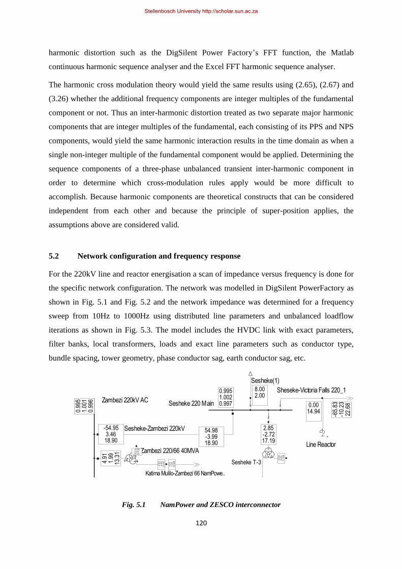
120
harmonic distortion such as the DigSilent Power Factory‟s FFT function, the Matlab
continuous harmonic sequence analyser and the Excel FFT harmonic sequence analyser.
The harmonic cross modulation theory would yield the same results using (2.65), (2.67) and
(3.26) whether the additional frequency components are integer multiples of the fundamental
component or not. Thus an inter-harmonic distortion treated as two separate major harmonic
components that are integer multiples of the fundamental, each consisting of its PPS and NPS
components, would yield the same harmonic interaction results in the time domain as when a
single non-integer multiple of the fundamental component would be applied. Determining the
sequence components of a three-phase unbalanced transient inter-harmonic component in
order to determine which cross-modulation rules apply would be more difficult to
accomplish. Because harmonic components are theoretical constructs that can be considered
independent from each other and because the principle of super-position applies, the
assumptions above are considered valid.
5.2 Network configuration and frequency response
For the 220kV line and reactor energisation a scan of impedance versus frequency is done for
the specific network configuration. The network was modelled in DigSilent PowerFactory as
shown in Fig. 5.1 and Fig. 5.2 and the network impedance was determined for a frequency
sweep from 10Hz to 1000Hz using distributed line parameters and unbalanced loadflow
iterations as shown in Fig. 5.3. The model includes the HVDC link with exact parameters,
filter banks, local transformers, loads and exact line parameters such as conductor type,
bundle spacing, tower geometry, phase conductor sag, earth conductor sag, etc.
Fig. 5.1 NamPower and ZESCO interconnector
Zambezi 220kV AC
0.99
51.
001
0.99
6
Sesheke 66 Main0 .9991 .0061 .000
Sesheke 220 Main
0.9951.0020.997
Sesheke 11 Main1 .0021 .0030 .996 Sesheke 66 Reserv e
0 .0000 .0000 .000
Sheseke-Victoria Falls 220_1
-65.
83-1
0.23
22.6
8
Sesheke-Zambezi 220kV-54.953.4618.90
54.98-3.9918.90 Line Reactor
0.0014.94
Senanga-S..
2.2
5-1
.26
6.9
4
Katima Mulilo-Zambezi 66 NamPowe..
4.9
11
.91
12
.98
Zambezi 220/66 40MVA
4.91
1.99
13.3
1
-4.9
1-1
.91
13
.31
-0 .000 .00
13.31
Sesheke(1)
8.002.00
Sesheke lo..
0 .600 .12
Sesheke T-3
2.85-2.7217.19
-2 .852 .74
17.19
-0.0
00
.00
17
.19
Ses
h..
0 .600 .136 .15
-0 .60-0 .126 .15 8
Km
Ove
rhe
ad
Lin
e
Ka
zu
ng
ula
-Se
sh
eke
66
1A
0 .00-1 .613 .07
Ka
tim
a M
ulilo
-Se
sh
eke
66
1A
Ka
tim
a M
ulilo
-Se
sh
eke
66
1A
0 .000 .000 .00
DIg
SIL
EN
T
Stellenbosch University http://scholar.sun.ac.za

121
Fig. 5.2 CLI HVDC model single line diagram (Courtesy NamPower / ABB)
Zambezi 220kV AC
Zambezi 330kV AC
Zam
bezi
330
kV H
VD
C
Ger
us 4
00kV
HV
DC
ElectrodeBus_Gerus ElectrodeBus_Zambezi
AC
Filte
rBus
_Ger
us_P
ole.
.
ACFi
lterB
us_Z
ambe
zi_P
ole.
.
BB Gerus
HP
3 F
ilte
r
1
Zambez i 330/220k V TR FR
0
Zambez i 330/220k V TR FRZambez i 330/220k V TR FR
Hp
32
filte
r11
DC
neut
ralC
ap_G
erus
_Pol
e1
1D
Cne
utra
lCap
_Zam
bezi
_Pol
e1 1
V
Sn
ub
be
rArr
est
er
Sn
ub
be
rArr
est
er
Ch
op
pe
rVa
lve
Ch
op
pe
rVa
lve
Ch
op
pe
rC
ho
pp
er
ConverterRes_Zambezi_Pole1ConverterRes_Zambezi_Pole1ConverterRes_Gerus_Pole1ConverterRes_Gerus_Pole1
Gerus HVDC 400kV BreakerGerus HVDC 400kV Breaker
Zambezi HVDC 330kV BreakerZambezi HVDC 330kV Breaker
SmoothReact_Gerus_Pole1SmoothReact_Gerus_Pole1SmoothReact_Zambezi_Pole1SmoothReact_Zambezi_Pole1
DCLine_Pole1DCLine_Pole1
Hp
3 fi
lter
1
Gro
un
d
IntA
CF
ilte
r_G
eru
s_P
ole
11
Gro
un
d_
Za
mb
ezi
HP
32
Filt
er
1
Trafo_Gerus_Pole17
Trafo_Gerus_Pole17
Trafo_Zambezi_Pole1
0
Trafo_Zambezi_Pole1
0
IntA
CF
ilte
r_Z
am
be
zi_
Po
le1
1
11
DCLine_Pole2DCLine_Pole2
Gro
un
d_
Ge
rus
DIg
SIL
EN
T
Stellenbosch University http://scholar.sun.ac.za

122
Fig. 5.3 Passive ZESCO network frequency response
The frequency response of this network configuration shows a parallel resonance point close
to the 4th harmonic order, a series resonance point close to the 5th harmonic order and other
dominant parallel resonance points close to the 9th and 17th harmonic orders. The major
players in these resonance points are the open-ended 224km long 220kV line between
Sesheke and Victoria Falls with 15MVAR line reactor and the HVDC scheme source
impedance with connected filter banks. Under normal circumstances, a parallel resonance
point close to the even-numbered 4th harmonic order would not be a great concern. However,
in this case it could prove to be an aspect to be reckoned with.
5.3 Simulated line and reactor energisation analysis
Since the local Katima Mulilo load was already energised by the HVDC converter station, the
inrush currents of the 220kV Sesheke Victoria Falls line with line reactor was investigated by
using a DigSilent EMT simulation to determine the nature of the inrush currents as it would
be without the VSC but only a normal external grid with equivalent source impedance and is
shown in Fig. 5.4:
Stellenbosch University http://scholar.sun.ac.za
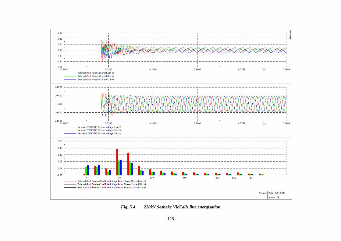
123
Fig. 5.4 220kV Sesheke VicFalls line energisation
Stellenbosch University http://scholar.sun.ac.za

124
The inrush currents were analysed in the frequency domain to reveal dominant harmonic
components. Among these, the 3rd and 4th harmonics were notably higher than the rest
during the transient condition. A proper harmonic sequence analysis of the current wave
shapes would give insight as to how these harmonic orders would cross-modulate via the
VSC. The continuous harmonic sequence analyser as developed for this thesis in Matlab was
used and yielded the following results as shown in Fig. 5.5:
Fig. 5.5 Line energisation harmonic sequence components
The phase sequence of the high 3rd and 4th harmonic orders can be identified as mostly PPS
but also with notable NPS components. Note the slow decaying DC component that contains
almost equal stationary NPS and PPS. These, together with the 2nd harmonic PPS and NPS
presence will have a definite effect on cross-modulated VSC harmonics.
Table 5.1 lists the expected cross-modulation effects as also shown in Fig. 2.23:
Stellenbosch University http://scholar.sun.ac.za
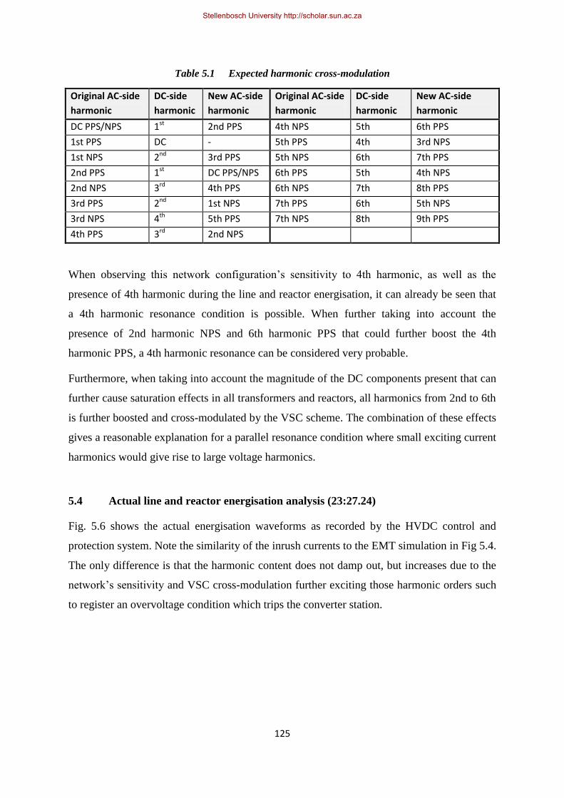
125
Table 5.1 Expected harmonic cross-modulation
Original AC-side
harmonic
DC-side
harmonic
New AC-side
harmonic
Original AC-side
harmonic
DC-side
harmonic
New AC-side
harmonic
DC PPS/NPS 1st 2nd PPS 4th NPS 5th 6th PPS
1st PPS DC - 5th PPS 4th 3rd NPS
1st NPS 2nd 3rd PPS 5th NPS 6th 7th PPS
2nd PPS 1st DC PPS/NPS 6th PPS 5th 4th NPS
2nd NPS 3rd 4th PPS 6th NPS 7th 8th PPS
3rd PPS 2nd 1st NPS 7th PPS 6th 5th NPS
3rd NPS 4th 5th PPS 7th NPS 8th 9th PPS
4th PPS 3rd 2nd NPS
When observing this network configuration‟s sensitivity to 4th harmonic, as well as the
presence of 4th harmonic during the line and reactor energisation, it can already be seen that
a 4th harmonic resonance condition is possible. When further taking into account the
presence of 2nd harmonic NPS and 6th harmonic PPS that could further boost the 4th
harmonic PPS, a 4th harmonic resonance can be considered very probable.
Furthermore, when taking into account the magnitude of the DC components present that can
further cause saturation effects in all transformers and reactors, all harmonics from 2nd to 6th
is further boosted and cross-modulated by the VSC scheme. The combination of these effects
gives a reasonable explanation for a parallel resonance condition where small exciting current
harmonics would give rise to large voltage harmonics.
5.4 Actual line and reactor energisation analysis (23:27.24)
Fig. 5.6 shows the actual energisation waveforms as recorded by the HVDC control and
protection system. Note the similarity of the inrush currents to the EMT simulation in Fig 5.4.
The only difference is that the harmonic content does not damp out, but increases due to the
network‟s sensitivity and VSC cross-modulation further exciting those harmonic orders such
to register an overvoltage condition which trips the converter station.
Stellenbosch University http://scholar.sun.ac.za

126
Fig. 5.6 Actual line energisation plots
Stellenbosch University http://scholar.sun.ac.za

127
The frequency response of the voltage waveforms from Fig. 5.6 as shown in Fig. 5.7 shows
the expected high 3rd and 4th harmonics. Note the relatively high 9th harmonic that makes
sense when looking at the network frequency response and the parallel resonance point close
to the 9th harmonic previously in Fig. 5.3.
Fig. 5.7 Actual line energisation AC-side harmonic components
Stellenbosch University http://scholar.sun.ac.za

128
The DC-side harmonics shown in Fig. 5.8 reveal a high fundamental component, as well as
high 2nd - 6th harmonic orders. These harmonic are cross-modulated from the AC-side
harmonic content as a result of the inrush current DC offset and other inrush and saturation
harmonic orders.
Fig. 5.8 Actual line energisation DC-side harmonic components
Stellenbosch University http://scholar.sun.ac.za

129
A continuous harmonic sequence component analysis of the recorded TFR reveals the
following results as shown in Fig. 5.9:
Fig. 5.9 Actual line energisation continuous harmonic sequence components
The constant presence of DC NPS and PPS with 2nd harmonic PPS explains DC-side
fundamental component. This effect could prolong transient and saturation conditions and
give rise to more harmonic content.
The increasing fundamental NPS component corresponds to the high DC-side 2nd harmonic
and increasing 3rd harmonic PPS. When investigating the HP3 filter that is supposed to cater
for 3rd harmonic PPS, it is found to be tuned at 115Hz which is closer to 2nd harmonic. Thus
the 3rd harmonic is not sufficiently damped but is allowed to grow.
The initial inrush currents contain all harmonic orders from 2nd to 7th. The initial presence of
4th harmonic PPS and NPS, boosted by more 4th
harmonic content originating from cross-
modulated 6th harmonic PPS and 2nd harmonic NPS interacts with the network parallel
resonance point that is close to 4th harmonic. Although the 4th harmonic NPS declines
slightly over time, the 4th harmonic PPS increases keeping the total 4th harmonic content
Stellenbosch University http://scholar.sun.ac.za

130
fairly stable although slightly increasing. This correlates with a slightly increasing DC-side
3rd harmonic. This exchange of NPS and PPS content is still to be examined.
The total harmonic content added to the fundamental component over the time period fulfils
the over-voltage tripping condition of the converter station at 1.25pu after 400ms.
5.5 PSCAD Electromagnetic Transient simulation
An EMT study was also conducted in PSCAD with the same detailed model that is used in
the RTDS system with the results shown in Fig. 5.10. The difference in this case is that the
energisation load selected to the various substations‟ loading points is the normal load which
is about 50MW compared to the 5MW energisation load in the actual case. The reasoning
behind this is to see if energising the line with normal load connected beforehand would help
to damp out some of the harmonic distortion effects.
The simulation time step was selected at 4µs as this gives a balance between high bandwidth
and valve firing accuracy, i.e. 125 times faster than valves switching at around 2kHz and the
amount of time consumed to complete a single simulation run of 2 to 5 seconds.
The detailed Caprivi Link model was used with the line parameters for the 220kV Zambezi
Sesheke line, 220kV 15MVAR line reactor, local transformers and loads, etc. Energising the
line and reactor yielded very much the same results as the actual energisation records and
DigSilent PF line energisation results when considering the line inrush current (320A peak)
and general wave shapes. The PSCAD results were written to a Comtrade format file for easy
external analysis.
Stellenbosch University http://scholar.sun.ac.za

131
Fig. 5.10 PSCAD VSC line energisation simulation
Stellenbosch University http://scholar.sun.ac.za

132
Fig. 5.11 PSCAD VSC with line energisation AC-side harmonic components
On closer inspection is evident that both the current and voltage harmonics are significantly
less due to the damping effect of the added load. Although the inrush current of the line and
line reactor is still the same, the continuation of the 3rd, 4th, 5th and 9th AC-side harmonics
Stellenbosch University http://scholar.sun.ac.za
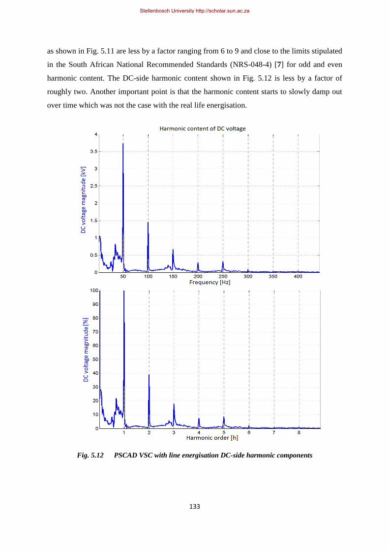
133
as shown in Fig. 5.11 are less by a factor ranging from 6 to 9 and close to the limits stipulated
in the South African National Recommended Standards (NRS-048-4) [7] for odd and even
harmonic content. The DC-side harmonic content shown in Fig. 5.12 is less by a factor of
roughly two. Another important point is that the harmonic content starts to slowly damp out
over time which was not the case with the real life energisation.
Fig. 5.12 PSCAD VSC with line energisation DC-side harmonic components
Stellenbosch University http://scholar.sun.ac.za
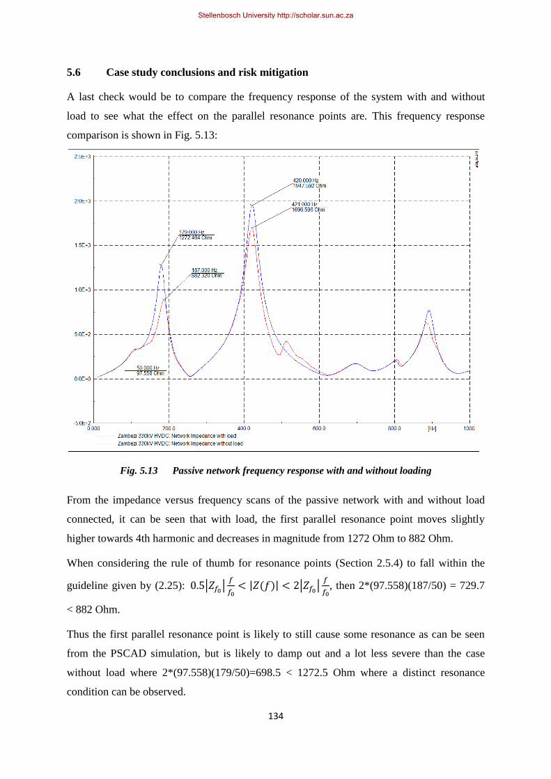
134
5.6 Case study conclusions and risk mitigation
A last check would be to compare the frequency response of the system with and without
load to see what the effect on the parallel resonance points are. This frequency response
comparison is shown in Fig. 5.13:
Fig. 5.13 Passive network frequency response with and without loading
From the impedance versus frequency scans of the passive network with and without load
connected, it can be seen that with load, the first parallel resonance point moves slightly
higher towards 4th harmonic and decreases in magnitude from 1272 Ohm to 882 Ohm.
When considering the rule of thumb for resonance points (Section 2.5.4) to fall within the
guideline given by (2.25):
, then 2*(97.558)(187/50) = 729.7
< 882 Ohm.
Thus the first parallel resonance point is likely to still cause some resonance as can be seen
from the PSCAD simulation, but is likely to damp out and a lot less severe than the case
without load where 2*(97.558)(179/50)=698.5 < 1272.5 Ohm where a distinct resonance
condition can be observed.
Stellenbosch University http://scholar.sun.ac.za

135
When the voltage harmonics between the two cases are compared, it can be seen that with
load less 3rd harmonic is observed in relation to the 4th harmonic. This can be attributed to
the parallel resonance point moving closer to 4th harmonic and further away from 3rd
harmonic.
The effects of harmonic cross-modulation by the VSC can be observed in both cases by the
extra harmonic orders generated around 3rd and 4th harmonic according to the harmonic
sequence components or the phase harmonics. The high fundamental component on the DC
side of the VSC for both cases indicates a risk of transformer saturation by DC components
produced by the VSC as a result of 2nd harmonic PPS inrush components.
The case of energising the network with load connected has been tested in real life as result
of a situation in the ZESCO network that necessitated NamPower to energise the line and line
reactor with the HVDC scheme. This time all loads were connected beforehand and after
energising the line and reactor, no tripping occurred as with the first case and thus no records
were generated indicating that any resonance condition damped out and did not grow to
register an overvoltage trip.
In general, it is advised not to energise the 220kV Sesheke - Victoria Falls line with line
reactor from the HVDC scheme due to the inrush harmonic components and cross-
modulation by the VSC. If absolutely necessary, it can be done but with all loads connected
where possible in order to bring more damping to the system.
Another mitigation technique would be to implement a modification to the HVDC control
system to allow manual operation of one of the two filter banks at the Zambezi converter
station. By switching in or out a filter intelligently, this would give some control over the
parallel resonant point frequency and damping. The feasibility of such a solution needs to be
studied further in more detail because it would imply removing the damping given by one of
the filter banks and thereby possibly sharpening the existing network parallel resonant points.
Stellenbosch University http://scholar.sun.ac.za

136
6 Results and conclusions
6.1 Overview of results and conclusions
In conclusion, although a fairly wide range of related fields had to be discussed in order to lay
the theoretical foundation and context for harmonic interaction between VSC HVDC and
weak AC systems, the theory in Chapter 3 and the application thereof in Chapter 4 and 5
could be focussed on strongly and explored in reasonable detail.
In Chapter 1, certain key questions were raised as well as objectives to be met in order to be
able answer these key questions. These objectives have been met by the various fields
discussed in the literature study in Chapter 2 from VSC systems, HVDC systems, VSC
switching theory and PWM switching techniques, power system harmonic principles,
harmonic sequence components, AC/DC harmonic interaction, simulation techniques and
simulation tools. This laid the foundation for Chapter 3 to further explore the fields of
harmonic sequence components, phase rotation in the frequency domain, VSC switching,
PWM and OPWM. The concept of HATR was introduced and the AC/DC HATR was
derived for different switching techniques. A new perspective was given by the examination
of harmonic cross-modulation by scheme characteristic harmonics. Chapter 4 made these
theories more practical by showing ways to model and simulate AC/DC harmonic interaction
and proving that the theories presented are valid. The case study in Chapter 5 confirmed that
the real life results are in line with the theories and simulations results presented. This chapter
aims to give a summary of these results and their significance to the industry.
The results and interpretations found in this thesis are spread throughout Chapters 2, 3, 4 and
5. Therefore a summary of the most important results are given in the next section.
6.2 Overview of important results
6.2.1 Harmonic sequence components
In Section 2.4.3, the harmonic dependent versus harmonic independent definition for the
operator and the validity for determining the sequence components of waveforms
containing harmonic content according to [31] - [34] as well as by Fortescue in [42] was
discussed and the case for a harmonic independent operator
was made. This
Stellenbosch University http://scholar.sun.ac.za

137
statement was further proved by the theory presented in Section 3.1.1 where the known
characteristic phase rotations for harmonics generation were confirmed.
The static harmonic sequence analyser developed in Excel, as well as the continuous
harmonic sequence analyser that was developed in Matlab, were based on the equations
presented in Section 3.1.1. All the simulation results exported from DigSilent PowerFactory
and PSCAD analysed in these two custom-made tools make perfect sense and align with the
theories presented in Section 3.2 and 3.3.
6.2.2 Identification of potentially dangerous series and parallel resonant points
The rule of thumb presented in Section 2.5.3 and Figure 2.14 to identify potentially
dangerous series or parallel resonance points by means of impedance versus frequency scans,
where no literature could be found to support its validity or invalidity, was shown to be
accurate in the conclusions of the case study in Section 5.6 at least for parallel resonance
points.
The understanding of the evaluation of impedance versus frequency sweeps is crucial in any
harmonic study including filter design. Movements in resonant points due to system
contingencies and fault level variations, as well as impedance magnification studies when
adding filter banks, is important to understand in order to avoid harmonic resonance
problems. Line energisation frequencies and possible inter-harmonic resonance conditions
also need to be considered.
6.2.3 Voltage Source Converter zero sequence elimination
The theory and equations presented in Section 3.2.1 to show that a VSC scheme does not
produce or transfer zero sequence components was confirmed by simulation study results.
The DC components transferred to the AC side of the VSC due to a DC-side fundamental
component are theoretically not of zero sequence order, but of equal stationary PPS and NPS
components as shown in the Matlab continuous harmonic sequence analyser. In the phase
domain, this relates to two positive DC phase quantities and one negative DC phase quantity
of double the amplitude of the other two phases. This challenges assumption that AC
transmission system DC components are only to be of zero sequence nature and is only true
for perfectly balanced flows.
Stellenbosch University http://scholar.sun.ac.za

138
6.2.4 Alternating Current / Direct Current harmonic interaction theory
The harmonic interaction theory and harmonic amplitude transfer ratios (HATRs) presented
in Section 3.3.1 for PWM and OPWM schemes were confirmed throughout Chapter 4 by
various Excel examples, DigSilent PowerFactory examples and a PSCAD example. Scheme
specific HATRs were confirmed and the attenuation for complete AC to DC to AC harmonic
transfers for higher order harmonics were discussed and attributed to DC-side frequency
response and DC-side filtering effect. The harmonic transfer rules were also confirmed by the
case study in Chapter 5 as a real life example of AC/DC harmonic interaction and resonance
with connected AC system. The role of the AC network frequency response with series and
parallel resonance points‟ effect on harmonic interaction that was highlighted in Section 3.3.1
can clearly be seen in the case study and network frequency response.
The presentation of the HATR concept, the deduction of the HATR formula for PWM
schemes and validity in simulations is a valuable concept for the study of AC/DC harmonic
interaction for VSC schemes.
6.2.5 Alternating Current/Direct Current harmonic interaction for modulation by
scheme characteristic harmonics
The assumptions made as presented in Section 2.7.2 and investigated in Section 3.3.2 has
opened a new world of harmonic interactions that are generally not noted in real life due to
the relatively low amplitudes of VSC scheme characteristic harmonics and AC-side
harmonics presented to the VSC scheme. Although these effects will be negligible in most
cases, they could start to play a role in case of low fault level AC systems coupled with a
strong VSC HVDC scheme in conjunction with other harmonic loads in the vicinity.
Harmonic amplification due to the presence of AC network series or parallel points could
pose some interesting scenarios.
Therefore this theory is valuable to take note of and to keep in mind when investigating
strange harmonic resonance cases involving VSC schemes and weak AC networks. The
presence of network unbalance and negative phase sequence components on the AC network
will also influence VSC positive phase sequence 3rd
harmonic generation and need to be kept
in mind since 3rd
harmonic components are normally assumed to be of zero sequence order.
The theory and equation (3.26) presented to determine harmonic cross-modulation by
components other than the fundamental component has been suggested in Section 3.3.2 and is
Stellenbosch University http://scholar.sun.ac.za

139
proved in concept by simulations performed in Excel and DigSilent PowerFactory in Section
4.4.
6.2.6 Modelling techniques and simulations
The modelling techniques and tools presented in Section 2.8 and Section 2.9 are further
discussed in Section 4.1 and are validated by the fact that the theories presented, the
simulations done for each theory and the case study results all line up very closely. This
shows the reliability and exactness of the simulation packages used and gives some comfort
to the concerns expressed in the beginning of Section 2.9.
However, the harmonic orders considered were limited to traditional lower order harmonics
below 25th
harmonic. Although the results for higher order harmonics may also have been
accurate, cognisance has been taken of the sampling rate (10kHz or 200 samples per 50Hz
cycle) of the real life transient fault records and accurate comparability to software simulation
outputs that may be of very high sampling rates (1MHz or 20000 samples per cycle) in order
to gain accurate valve switching instants for harmonic interaction results.
6.2.7 Case study results
Although the case study results have been discussed in Section 5.6, it gives a satisfying
conclusion to the important role system damping plays in the proliferation of power system
harmonics and the importance of impedance versus frequency sweep studies.
It shows that although AC/DC harmonic interaction is an effect to be reckoned with
especially with weak AC systems and that it does not only exist in theory. Yet the case study
shows that it can be mitigated to some extent by understanding the connected AC systems
and resonant sensitivities and it highlights that operational regimes can often be used to
mitigate certain risks if they have not been identified during a design or conceptualisation
process.
Often a harmonic integration study cannot beforehand, often a few years in advance, cater for
all future developments and all possible contingencies. In that case, new ways need to be
found to mitigate harmonic problems with the least cost implications such as operational
regimes, filter banks, gradual increase in fault level as system develops, etc.
Stellenbosch University http://scholar.sun.ac.za

140
6.3 Future work on Alternating Current / Direct Current harmonic interaction
Although this thesis started to open the world of harmonic cross-modulation for VSC
schemes, there are still many aspects that can be studied in order to make the picture of
AC/DC harmonic interaction more complete:
The relative phase angles of harmonic orders transferred from the AC- to DC side and
back to the AC side can be investigated to determine if transferred harmonics will add in
phase or in another relation to one-another especially when considering harmonic
interaction due to scheme characteristic harmonics and other pre-existing AC-side
harmonics.
The HATR derivation for modulation by scheme characteristic harmonics can be
investigated if deemed relevant for practice.
The effect of third harmonic injection on PWM schemes‟ HATR can be investigated.
HATR equations considering DC-side frequency response could be investigated to
incorporate the typical effects of DC-side capacitance.
Higher order harmonic measurement techniques is a separate field, but could be relevant
considering that many higher order harmonic components are difficult to accurately
measure in order to make good comparisons with simulation results.
Control strategies and effect of OPWM to minimize harmonic content could be
investigated to see if cross-modulated harmonic orders that are programmed to be
eliminated by OPWM strategies are actually eliminated, or if harmonic cross-modulation
bypasses this mechanism.
Harmonic interaction can also be investigated for different VSC configurations especially
considering multi-level bridge configurations.
Frequency injections other that integer multiples of the fundamental components, such as
frequencies in the SSR range can be investigated to determine the wide band response of
VSC schemes as it relates to cross-modulation and frequency interaction.
The development of software tools suitable for the continuous harmonic sequence analysis
of multiple transient inter-harmonic distortions can be investigated. One option could be to
use the DWT as the basis of analysis.
Stellenbosch University http://scholar.sun.ac.za

141
6.4 Recommendations and final conclusion
Although the pursuit of a deeper theoretical understanding of the mechanisms behind
harmonic interaction is valid, sight should not be lost of the real life practical implications.
Some aspects are very relevant and need to be taken into account. For other aspects, where
the accuracy and dependability of field measurements become realistically doubtful and
where the level of relative harmonic quantities become too small and insignificant to be
meaningful, a reality check may be required. Yet, the point where theoretically interesting
and practically relevant become mutually exclusive is not always so clear especially given the
great variations in fault level and network characteristics encountered in transmission systems
all over the world.
In conclusion, it can be said that power systems harmonic analysis and the search for
solutions and mitigations is not always simple and straightforward and is by some considered
not only a science, but also an art where at the end, years of experience in the field backed by
a solid theoretical foundation is the best teacher.
Stellenbosch University http://scholar.sun.ac.za

142
7 References
[1] NamPower. (2011) Short term critical supply project. Presentation.
[2] T.G. Magg, E. Krige, M. Manchen, J. Wasborg, and J. Sundin, "Connecting networks
with VSC HVDC in Africa: Caprivi Link Interconnector," in IEEE PES PowerAfrica
2012 Conference and Exposition, Johannesburg, 2012.
[3] AE-Africa. (2011, April) Alternative Energy Africa Publications. [Online]. http://ae-
africa.com/read_article.php?NID=2889
[4] T.G. Magg, M. Manchen, J. Wasborg, E. Krige, and H. D. Mutschler, "Caprivi Link
Interconnector: The first VSC HVDC power transmission with overhead lines," in
CIGRE B4 Colloquium, Sydney, Paper 29, 20 October 2011.
[5] M. Bongiorno, S. Lundberg L. Harnefors, "Input-admittance calculation and shaping for
controlled Voltage Source Converters," IEEE Transactions on Industrial Electronics,
vol. 54, no. 6, December 2007.
[6] A. P. J. Rens, "Validation of popular non-sinusoidal power theories for the analysis and
management of modern power systems," Ph.D. dissertation, Electrical Engineering,
North-West University, Potchefstroom, South Africa, 2005.
[7] "SABS Standards Division, Electricity Supply - Quality of Supply, Part 4: Application
practices for licensees," NRS048-4, Ed. 2, 2009.
[8] G. J. Wakileh, Power Systems Harmonics, Fundamentals, Analysis and Filter design.
Germany: Springer, 2001.
[9] Index Mundi. [Online]. http://www.indexmundi.com/namibia/area.html
[10] Y. Jiang, "Active and Reactive Power Control for Transmission Systems with Voltage
Source Converters," Ph.D. dissertation, Royal Institute of Technology, Stockholm, 1997.
[11] G. Reed, R. Pape, and M. Takeda, "Advantages of Voltage Sourced Converter (VSC)
based design concepts of FACTS and HVDC-link applications," in Power Engineering
Society General Meeting, 2003, IEEE, vol. 3, 2003.
Stellenbosch University http://scholar.sun.ac.za

143
[12] J. Arrillaga and N. R. Watson, Power System Harmonics, 2nd ed. Chichester, England:
John Wiley & Sons, Ltd, 2003.
[13] E. Krige, NamPower Utility Experiences, available from author, 2004-2012.
[14] J. Arrilaga, High Voltage Direct Current Transmission, 2nd ed. London, United
Kingdom: IEE Power and Energy Series 29, 1998.
[15] Wikipedia, The free encyclopedia. [Online]. www.wikipedia.com at 2011-11-09.
[16] P. Kundur, Power System Stability and Control, N. J. Balu (The EPRI Power System
Engineering Series), Ed. United States of America: McGraw-Hill, Inc, 1994.
[17] J. D. Glover and M. Sarma, Power System Analysis and Design, 2nd ed. Boston: PWS
Publishing Company, 1994.
[18] P.K. Steimer, H. Grüning, J. Werninger, and D. Schröder, "State of the art verification of
the Hard Driven GTO Inverter development for a 100MVA Intertie," IEEE Transactions
on Power Electronics, vol. 13, no. 6, pp. 1182 - 1190, 1998.
[19] J.P. Ballad, R.J. Bassett, and C.C. Davidson, "Power Electronic Devices and their impact
for Power Transmission," in 6th International Conference on AC and DC Power
Transmission, IEE Conference Publication No. 423, 1996.
[20] L. Gyugyi, "Dynamic Compensation of AC Transmission Lines by Solid-state
Synchronous Voltage Sources," IEEE Transactions on Power Delivery, vol. 9, no. 2,
April 1994, pp. 904 - 911.
[21] E. Larsen, N. Miller, S. Nilsson, and S. Lindgren, "Benefits of GTO-based compensation
systems for electrical utility applications," IEEE Transactions on Power Delivery, vol. 7,
no. 4, pp. 2056 - 2064, October 1992.
[22] D.G. Holmes and T.A. Lipo, Pulse width modulation for power converters: principles
and practice, M. E. El-Hawary, Ed. New Jersey, USA: IEEE Series on Power
Engineering, IEEE Press, J. Wiley and Sons, 2003.
[23] D. L. H. Aik, "Methods for voltage and power stability analysis of emerging HVDC
system configurations," in International Conference on Power System Technology, vol.
1, 2000, pp. 409-414.
Stellenbosch University http://scholar.sun.ac.za

144
[24] D.J. Melvold, T. Endo, and H.P. Lips, "Effects of operating configurations of multi-
terminal HVDC systems on dc filter performance," IEEE Transactions on Power
Delivery, vol. PWRD-2, no. 3, July 1987.
[25] K. Sadek, M. Pereira, D.P. Brandt, A.M. Gole, and A. Daneshpooy, "Capacitor
Commutated Converter Circuit Configurations," IEEE Transactions on Power Delivery,
vol. 13, no. 4, pp. 1257-1264, October 1998.
[26] "CIGRE Protocol for Reporting the Operational Performance of HVDC Transmissions
Systems," Working Group 14.04, March 2008.
[27] "IEEE Guide for the Evaluation of the Reliability of HVDC Converter Stations," IEEE
Std 1240-2000, R2006.
[28] N. Mohan, T. M. Undeland, and W. P. Robbins, Power Electronics - Converters,
Applications, and Design, 2nd ed. United States of America: John Wiley & Sons. Inc,
1995.
[29] L. Carlsson; G. Asplund; H. Bjorklund; H. Stomberg;, "Recent and future trends in
HVDC converter station design," in IEE 2nd International Conference on Advances in
Power System Control, Operations and Management, Hong Kong, 1993, pp. 221-226.
[30] R. E. Betz, C. Townsend, T. J. Summers, and G. Mirzaeva, "Simultaneous estimation of
sequence and harmonic components for StatCom applications," in 14th Annual
Internation Power Electronics and Motion Control Conference, EPE-PEMC, 2010, pp.
T7-47 - T7-54.
[31] B. C. Smith, N. R. Watson, A. R. Wood, and J. Arrillaga, "A sequence components
model of the AC / DC converter in the harmonic domain," IEEE Transactions on Power
Delivery, vol. 12, no. 4, pp. 1736 - 1743, October 1997.
[32] M. T. Hartman, "The application of Fortesque's transformation to describe power states
in multiphase circuits with non-sinusoidal voltage and currents," in 9th International
Conference, Electrical Power Quality and utilisation, Barcelona, October 2007, pp. 1-6.
[33] S. M. Deckman and E. F. Melo, "On-line evaluation of voltage quality indexes for
harmonic distoration, flicker, and sequence components," in 8th International
Conference on Harmonics And Quality of Power, SP, Brazil, 1998, pp. 549 - 554, Vol1.
Stellenbosch University http://scholar.sun.ac.za
145
[34] A. Baggini, Handbook of power quality. Chichester, United Kingdom: John Wiley &
Sons, Ltd, 2008.
[35] IEEE Interharmonic Task Force, "Interharmonics in Power Systems," Cigre
36.05/CIRED 2 CC02 Voltage Quality Working Group, 1997.
[36] L. F. Beites, J. G. Mayordomo, A. Hernandez, and R. Asensi, "Harmonics,
interharmonics, and unbalances of arc furnaces: A new frequency domain approach,"
IEEE Transactions on Power Delivery, vol. 16, no. 4, p. 661, October 2001.
[37] J. Fourier, "The analytical theory of heat," Cambridge University Press, 1978.
[38] S. Haykin, Introduction to analog and digital communications. New York, United States
of America: John Wiliey and Sons, Inc, 1989.
[39] J. A. Glassman, "A generalization of the Fast Fourier Transform," IEEE Transactions on
Computers, vol. C-19, no. 2, pp. 105 - 116, February 1970.
[40] "IEEE Recommended Practice for Industrial and Commercial Power Systems Analysis,"
IEEE Std 399, 1997.
[41] F. Neves et al., "A Space-vector Discrete Fourier Transform for Detecting Harmonic
Sequence Components of Three-Phase Signals," in 35th Annual Conference of IEEE
Industrial Electronics, 2009, pp. 3631 - 3636.
[42] C.L. Fortescue, "Method of Symmetrical co-ordinates applied to the solution of
polyphase networks," Transactions of the American Institute of Electrical Engineers,
vol. 37, no. 2, pp. 1027 - 1140, 1918.
[43] Y. M. Chen, "Passive filter design using genetic algorithms," IEEE Transactions on
Industrial Electronics, vol. 50, no. 1, pp. 202-207, February 2003.
[44] F.Z. Peng, H. Akagi, and A. Nabae, "A new approach to harmonic compensation in
power systems-a combined system of shunt passive and series active filters," IEEE
Transactions on Industry Applications, vol. 26, no. 6, pp. 983 - 990, 1990.
[45] M.M. Zakaria Moustafa and S. Filizadeh, "Simulation of a VSC transmission scheme
supplying a passive load," in 34th Annual Conference of IEEE Industrial Electronics,
2008, pp. 942 - 946.
Stellenbosch University http://scholar.sun.ac.za
146
[46] J. Holtz, "Pulsewidth Modulation-A Survey ," IEEE Transactions on Industrial
Electronics, vol. 39, no. 5, pp. 410 - 420 , 1992.
[47] J. E. Chen and T. J. Liang, "A Novel Algorithm in Solving Nonlinear Equations for
Programmed PWM Inverter to Eliminate Harmonics," in 23rd International Conference
on Industrial Electronics, Control and Instrumentation , Ta-hsu Hsiang, Kaohsiung
Country, Taiwan, 1997, pp. 698 - 703 vol.2.
[48] Z. Du, L.M. Tolbert, and J.N. Chiasson, "Harmonic elimination for multilevel converter
with programmed PWM method ," in 39th IEEE Industry Applications Conference,
2004, pp. 2210 - 2215 vol.4.
[49] A. M. Trzynadlowski, F. Blaabjerg, J. K. Pedersen, R. L. Kirklin, and S. Legowski,
"Random Pulse Width Modulation Techniques for Converter-Fed Drive Systems - A
Review," IEEE Transactions On Industry Applications, vol. 30, no. 5, pp. 1166 - 1175,
September / October 1994.
[50] DigSilent GmbH, PowerFactory Technical Documentation, Build 511., March 2011.
[51] Manitoba HVDC Research Centre Inc, Applications of PSCAD / EMTDC., 2007.
[52] Z. Bo and L. Tiecheng, "Application of Nonlinear Dynamic on Ferroresonance," in
Engineering Conference, Asia-Pacific, 2009, pp. 1-4.
[53] J. Watson, N.R. Arrillaga, "The Harmonic Domain Revisited," in 13th International
Conference on Harmonics and Quality of Power, Wollongong, 2008, pp. 1-9.
[54] W. Wiechowski, J. Lykkegaard, B. Bak-Jensen, and C. L. Bak, "Hybrid time/frequency
domain modelling of nonlinear components," in 9th International Conference, Electrical
Power Quality and Utilisation, Barcelona, 9-11 October 2007, pp. 1-6.
[55] J. Arrillaga, A. Medina, M. L. V. Lisboa, M. A. Cavia, and P. Sanchez, "The harmonic
domain: A frame of reference for power system harmonic analysis," IEEE Transactions
on Power Systems, vol. 10, no. 1, pp. 443-440, February 1995.
[56] B.C. Smith, J. Arrillaga, A.R. Wood, and N.R. Watson, "A review of iterative harmonic
analysis for AC-DC power systems," IEEE Transactions on Power Delivery, vol. 13, no.
1, pp. 180-185, January 1998.
Stellenbosch University http://scholar.sun.ac.za

147
[57] M.A.A. Lima, J.R. de Carvalho, D.V. Coury, A.S. Cerqueira, and C.A. Duque, "A
method of dynamic resampling for DFT-based harmonic analysis under time-varying
frequency conditions," in 14th International Conference on Harmonics and Quality of
Power (ICHQP), 2010, pp. 1-6.
[58] M. A. Cody, "The Fast Wavelet Transform," Dr. Dobb's Journal, April 1992.
[59] Z Xiang and Y Lu, "A study of the fast wavelet transform method in computational
electromagnetics," IEEE Transactions on Magnetics, vol. 34, no. 5, pp. 3323 - 3326,
1998.
[60] H. W. Dommel, "Digital computer solution of electromagnetic transients in single- and
multiphase networks," IEEE Transactions on Power Apparatus and Systems, vol. PAS-
88, no. 4, pp. 388 - 399, April 1969.
[61] RTDS Technologies Inc. [Online]. http://www.rtds.com at 2011-12-02
[62] Mathworks. [Online]. http://www.mathworks.com at 2011-12-02
[63] MathCad. [Online]. http:///www.ptc.com/products/mathcad/ at 2011-12-02
[64] Excel for Engineers. [Online]. http://www.engineers-excel.com at 2011-12-02
[65] Lindo64. [Online]. http://www.lindo.com/ at 2011-12-02
Stellenbosch University http://scholar.sun.ac.za

148
Appendix A – Harmonic sequence analyser code
% Precise Harmonic analyse for positive, negative and zero sequence
% components up to 30*F1 Hz, The sampling frequency should not be slower
% than F1*100 provided Ying Jiang_Häfner 200706
% Modified by E.Krige 20110315 for continuous harmonic sequence plots
% for harmonic components h=0,1,2,...11
clear
a=comtrade %load the TFR to be analysed
%
ss=7000; % select a starting point for harmonic analyse S=tstart/Tsample
Tsample=0.0001
Swin=30 %Total cycles to analyse
for count = 1:Swin
Ss=Sss+((count-1)*200); % select a starting point for harmonic analyse S=tstart/Tsample
Se=Ss+200 ; % manual setting (200=1period)
Xp(count)=(count-1)*0.02 % Time axis from starting point
upcat=a.aCh(9).d; % "1" should be the channel number in TFR for the analysed variable
phase a
uLa=upcat([Ss:1:Se]);
upcbt=a.aCh(10).d; % "2" should be the channel number in TFR for the analysed variable
phase b
uLb=upcbt([Ss:1:Se]);
upcct=a.aCh(11).d; % "3" should be the channel number in TFR for the analysed variable
phase c
uLc=upcct([Ss:1:Se]);
tplot=[Ss:1:Se]*Tsample;
ZuLa=fft(uLa)/length(uLa);
ZuLb=fft(uLb)/length(uLb);
ZuLc=fft(uLc)/length(uLc);
%
i=sqrt(-1);
r1=cos(2*pi/3)+i*sin(2*pi/3);
r2=cos(4*pi/3)+i*sin(4*pi/3);
%
ZLP=(1/3)*2*(ZuLa([1:12])+r1*ZuLb([1:12])+r2*ZuLc([1:12]));
Stellenbosch University http://scholar.sun.ac.za

149
ZLN=(1/3)*2*(ZuLa([1:12])+r2*ZuLb([1:12])+r1*ZuLc([1:12]));
ZLO=(1/3)*2*(ZuLa([1:12])+ZuLb([1:12])+ZuLc([1:12]));
Z1P(count)=abs(ZLP(1));
Z1N(count)=abs(ZLN(1));
Z10(count)=abs(ZLO(1));
Z2P(count)=abs(ZLP(2));
Z2N(count)=abs(ZLN(2));
Z20(count)=abs(ZLO(2));
Z3P(count)=abs(ZLP(3));
Z3N(count)=abs(ZLN(3));
Z30(count)=abs(ZLO(3));
Z4P(count)=abs(ZLP(4));
Z4N(count)=abs(ZLN(4));
Z40(count)=abs(ZLO(4));
Z5P(count)=abs(ZLP(5));
Z5N(count)=abs(ZLN(5));
Z50(count)=abs(ZLO(5));
Z9P(count)=abs(ZLP(9));
Z9N(count)=abs(ZLN(9));
Z90(count)=abs(ZLO(9));
Z6P(count)=abs(ZLP(6));
Z6N(count)=abs(ZLN(6));
Z60(count)=abs(ZLO(6));
Z7P(count)=abs(ZLP(7));
Z7N(count)=abs(ZLN(7));
Z70(count)=abs(ZLO(7));
Z8P(count)=abs(ZLP(8));
Z8N(count)=abs(ZLN(8));
Stellenbosch University http://scholar.sun.ac.za
150
Z80(count)=abs(ZLO(8));
end;
figure
subplot(811), plot(Xp,Z1N,Xp,Z1P,Xp,Z10)
legend('DC NPS','DC PPS','DC ZPS')
grid
title('Harmonic sequence components (Ipcc)');
subplot(812), plot(Xp,Z2P,Xp,Z2N,Xp,Z20)
legend('1st PPS','1st NPS','1st ZPS')
grid
subplot(813), plot(Xp,Z3P,Xp,Z3N,Xp,Z30)
legend('2nd PPS','2nd NPS','2nd ZPS')
grid
subplot(814), plot(Xp,Z4P,Xp,Z4N,Xp,Z40)
legend('3rd PPS','3rd NPS','3rd ZPS')
grid
subplot(815), plot(Xp,Z5P,Xp,Z5N,Xp,Z50)
legend('4th PPS','4th NPS','4th ZPS')
grid
subplot(816), plot(Xp,Z6P,Xp,Z6N,Xp,Z60)
legend('5th PPS','5th NPS','5th ZPS')
grid
subplot(817), plot(Xp,Z7P,Xp,Z7N,Xp,Z70)
legend('6th PPS','6th NPS','6th ZPS')
grid
subplot(818), plot(Xp,Z7P,Xp,Z7N,Xp,Z70)
legend('7th PPS','7th NPS','7th ZPS')
grid
Stellenbosch University http://scholar.sun.ac.za

151
Appendix B – Case study event list
Date Time Station Group Event Status
20101005 23:16:54.000 GERUS CVR CONDITION RFE AC Voltage Healthy Alarm
20101006 23:16:54.176 ZBEZI 220 ALARMS 50V Charger Charge Unh Alarm
20101005 23:16:54.542 ZBEZI CVR P1 TRF 330 ANALOG BB2 kV Low Alarm
20101005 23:16:54.924 ZBEZI CVR ALARMS Fast Stop Activated Alarm
20101005 23:16:55.000 ZBEZI CVR CNTRL MDE Passive/Normal Network Indic Passive
20101005 23:16:55.000 GERUS CVR CONDITION RFO TapChanger RFO Normal
20101005 23:16:55.000 GERUS CVR CONDITION RFE AC Voltage Healthy Normal
20101005 23:16:55.339 ZBEZI CVR ALARMS AC Hall Cooling Alarm Alarm
20101005 23:16:55.362 ZBEZI CVR ALARMS Valve Cooling Faulty Sensor Alarm
20101005 23:16:55.379 ZBEZI CVR ALARMS Reactor Hall Cooling Failure Alarm
20101006 23:16:56.911 SESHEKE 220 ZAMB BREAKER Breaker position indication Open
20101006 23:16:58.357 ZBEZI 220 ALARMS 50V Charger Charge Unh Normal
20101005 23:16:56.714 ZBEZI CVR P1 TRF 330 ANALOG BB2 kV Normal
20101005 23:16:58.000 GERUS CVR CONDITION RFO TapChanger RFO Alarm
20101005 23:16:58.554 ZBEZI CVR ALARMS Valve Cooling Faulty Sensor Normal
20101005 23:17:01.683 GERUS 220 220 OMBUR ANALOGS MVAr Normal
20101005 23:17:02.171 ZBEZI CVR ALARMS Valve Cooling Urg Alarm
20101005 23:17:06.587 ZBEZI CVR ALARMS Valve Cooling Urg Normal
20101005 23:19:44.433 ZBEZI 220 220 SESHE ANALOGS kV Low Alarm
20101005 23:19:44.433 ZBEZI 220 220 SESHE ANALOGS MVAr High Alarm
20101005 23:19:44.433 ZBEZI 220 66 BB1 ANALOGS kV Low Alarm
20101005 23:19:44.433 ZBEZI 220 220 SESHE ANALOGS kV Normal
20101005 23:20:04.558 ZBEZI 220 66 BB1 ANALOGS kV Normal
20101005 23:20:04.558 ZBEZI 220 220 SESHE ANALOGS MVAr Normal
20101005 23:20:04.558 SESHEKE 66 KATIMA ANALOGS kV Low Alarm
20101005 23:21:07.292 SESHEKE 66kV BBV ANALOGS kV Low Alarm
20101005 23:21:07.292 SESHEKE 220 VICFAL ANALOGS kV Low Alarm
20101005 23:21:55.339 ZBEZI CVR ALARMS AC Hall Cooling Failure Alarm
20101005 23:27:24.656 SESHEKE 220 ZAMB BREAKER Breaker position indication Closed
20101005 23:27:24.909 ZBEZI CVR ALARMS AC Bus Prot Unh Alarm
20101005 23:27:24.946 ZBEZI CVR ALARMS AC Yard W2.W1.Q1 BKR Unh Alarm
20101005 23:27:24.948 ZBEZI CVR ALARMS AC Yard Brkr Unsynchr Oper Alarm
20101005 23:27:24.948 ZBEZI CVR ALARMS DC Yard P1.WP.Q3 Fail Alarm
20101005 23:27:24.950 ZBEZI CVR ALARMS DC Yard P1.WP.Q2 Fail Alarm
20101005 23:27:24.952 ZBEZI CVR ALARMS DC Yard P1.WP.Q4 Fail Alarm
20101005 23:27:24.952 ZBEZI CVR ALARMS AC Bus Prot Unh Normal
20101006 23:27:24.956 ZBEZI 220 ALARMS 50V Charger Charge Unh Alarm
20101005 23:27:24.964 ZBEZI CVR P1 TRF 330kV BKR Breaker position indication Open
20101005 23:27:24.965 ZBEZI CVR ALARMS AC Yard W2.W3.Q1 BKR Unh Alarm
20101005 23:27:24.967 ZBEZI CVR ALARMS AC Yard W2.W2.Q1 BKR Unh Alarm
Stellenbosch University http://scholar.sun.ac.za

152
20101005 23:27:24.967 ZBEZI CVR ALARMS DC Yard P1.WP.Q1.Q1 Fail Alarm
20101005 23:27:24.971 ZBEZI CVR P1_H60FIL BREAKER Breaker position indication Open
20101005 23:27:24.976 ZBEZI CVR ALARMS AC Yard P1.Z2.Q1 BKR Unh Alarm
20101005 23:27:24.977 ZBEZI CVR ALARMS AC Yard W2.W3.Q2 BKR Unh Alarm
20101005 23:27:24.991 ZBEZI CVR FLTR 3P1 330kV BKR Breaker position indication Open
20101005 23:27:24.994 ZBEZI CVR ALARMS Aux Power LV Sw/gear Unh Alarm
20101005 23:27:24.995 ZBEZI CVR FLTR 32P1 330kV BKR Breaker position indication Open
20101005 23:27:25.000 ZBEZI CVR SEQUENCE P1 Conv Blocked Status Blocked
20101005 23:27:25.000 GERUS CVR CONDITION RFE AC Voltage Healthy Alarm
20101005 23:27:25.000 ZBEZI CVR SEQUENCE P1 Conv TRF Breakers Status Open
20101005 23:27:25.000 GERUS CVR CONDITION RFE AC Voltage Healthy Normal
20101005 23:27:25.017 ZBEZI CVR ALARMS AC Yard Brkr Unsynchr Oper Normal
20101005 23:27:25.620 ZBEZI CVR P1 TRF 330 ANALOG BB2 kV Low Alarm
20101005 23:27:25.690 ZBEZI CVR ALARMS Cnvter TRF Transform Dryer Alarm
20101005 23:27:26.012 ZBEZI CVR ALARMS Valve Cooling Faulty Sensor Alarm
20101005 23:27:26.040 ZBEZI CVR P1 TRF 330RES BKR Breaker position indication Open
20101005 23:27:26.634 ZBEZI CVR ALARMS Valve Cooling Power Faulty Alarm
20101005 23:27:27.954 ZBEZI CVR ALARMS Cnvter TRF Aux Supply Unh Alarm
20101005 23:27:36.691 ZBEZI CVR ALARMS Valve Cooling Urg Alarm
20101005 23:27:41.855 ZBEZI CVR ALARMS AC Yard P1.Z2.Q1 BKR Unh Normal
20101005 23:27:41.856 ZBEZI CVR ALARMS DC Yard P1.WP.Q1.Q1 Fail Normal
20101005 23:27:41.856 ZBEZI CVR ALARMS DC Yard P1.WP.Q2 Fail Normal
20101005 23:27:41.856 ZBEZI CVR ALARMS AC Yard W2.W2.Q1 BKR Unh Normal
20101005 23:27:41.856 ZBEZI CVR ALARMS AC Yard W2.W3.Q1 BKR Unh Normal
20101005 23:27:41.857 ZBEZI CVR ALARMS DC Yard P1.WP.Q3 Fail Normal
20101005 23:27:41.857 ZBEZI CVR ALARMS DC Yard P1.WP.Q4 Fail Normal
20101005 23:27:41.857 ZBEZI CVR ALARMS AC Yard W2.W3.Q2 BKR Unh Normal
20101005 23:27:41.858 ZBEZI CVR ALARMS AC Yard W2.W1.Q1 BKR Unh Normal
20101005 23:27:41.874 ZBEZI CVR ALARMS Valve Cooling Power Faulty Normal
20101005 23:27:42.402 ZBEZI CVR ALARMS Cnvter TRF Aux Supply Unh Normal
20101005 23:27:43.024 ZBEZI CVR ALARMS Cnvter TRF Transform Dryer Normal
20101005 23:27:43.667 ZBEZI CVR ALARMS Aux Power LV Sw/gear Unh Normal
20101005 23:27:49.636 ZBEZI CVR P1 TRF TC POS IND Tap position 22
20101005 23:27:56.589 ZBEZI CVR P1 TRF TC POS IND Tap position 23
20101005 23:28:02.347 ZBEZI CVR ALARMS Valve Cooling Faulty Sensor Normal
20101005 23:28:03.136 ZBEZI CVR P1 TRF TC POS IND Tap position 24
20101005 23:28:09.667 ZBEZI CVR P1 TRF TC POS IND Tap position 25
20101005 23:30:02.526 ZBEZI 220 66 BB1 ANALOGS kV Low Alarm
20101005 23:30:02.526 ZBEZI 220 220 BB2 ANALOGS kV Low Alarm
20101005 23:30:02.526 ZBEZI 220 220 SESHE ANALOGS kV Low Alarm
20101005 23:30:32.050 ZBEZI CVR ALARMS Valve Cooling Urg Normal
20101005 23:36:01.495 ZBEZI CVR CNTRL MDE Reduced UDC Cmd Selected
20101005 23:36:02.495 ZBEZI CVR CNTRL MDE Reduced UDC Cmd Activate
20101005 23:38:52.507 ZBEZI CVR ALARMS AC Hall Cooling Failure Normal
Stellenbosch University http://scholar.sun.ac.za
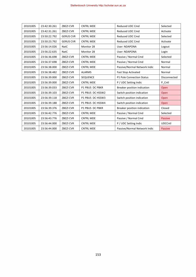
153
20101005 23:42:30.261 ZBEZI CVR CNTRL MDE Reduced UDC Cmd Selected
20101005 23:42:31.261 ZBEZI CVR CNTRL MDE Reduced UDC Cmd Activate
20101005 23:50:22.792 GERUS CVR CNTRL MDE Reduced UDC Cmd Selected
20101005 23:50:23.792 GERUS CVR CNTRL MDE Reduced UDC Cmd Activate
20101005 23:56:14.026 NatC Monitor 28 User: NDAPONA Logout
20101005 23:56:22.635 NatC Monitor 28 User: NDAPONA Login
20101005 23:56:36.698 ZBEZI CVR CNTRL MDE Passive / Normal Cmd Selected
20101005 23:56:37.698 ZBEZI CVR CNTRL MDE Passive / Normal Cmd Normal
20101005 23:56:38.000 ZBEZI CVR CNTRL MDE Passive/Normal Network Indic Normal
20101005 23:56:38.482 ZBEZI CVR ALARMS Fast Stop Activated Normal
20101005 23:56:39.000 ZBEZI CVR SEQUENCE P1 Pole Connection Status Disconnected
20101005 23:56:39.000 ZBEZI CVR CNTRL MDE P / UDC Setting Indic P_Cntl
20101005 23:56:39.033 ZBEZI CVR P1 PBUS DC PBKR Breaker position indication Open
20101005 23:56:39.103 ZBEZI CVR P1 PBUS DC HSSW2 Switch position indication Open
20101005 23:56:39.118 ZBEZI CVR P1 PBUS DC HSSW3 Switch position indication Open
20101005 23:56:39.188 ZBEZI CVR P1 PBUS DC HSSW4 Switch position indication Open
20101005 23:56:39.376 ZBEZI CVR P1 PBUS DC PBKR Breaker position indication Closed
20101005 23:56:42.776 ZBEZI CVR CNTRL MDE Passive / Normal Cmd Selected
20101005 23:56:43.776 ZBEZI CVR CNTRL MDE Passive / Normal Cmd Passive
20101005 23:56:44.000 ZBEZI CVR CNTRL MDE P / UDC Setting Indic UDCCntl
20101005 23:56:44.000 ZBEZI CVR CNTRL MDE Passive/Normal Network Indic Passive
Stellenbosch University http://scholar.sun.ac.za

154
Appendix C – Complex vector, Clarke’s ( ) components and d-q
components
C.1) Complex vector
Let
The purpose of the complex vector notation as defined by (C1) is to be able to represent a
three-phase system comprising of three sinusoidal quantities as a single rotating vector. The
complex vector, also known as the space vector, is chosen such that the three-phase
instantaneous quantities are projected to three orthogonal axes
. [10],
[22].
and
Projecting all three phases on the reference phase “a” gives the following results:
Let
then
Stellenbosch University http://scholar.sun.ac.za

155
C.2) -components
The and components are defined as the real and imaginary components of the complex
vector [10] as given by the relationship
where
and
C.3) - components
In order to achieve a static reference frame from a rotating reference frame, the d-q
components can be used [10] by using the relationship
where
and
Stellenbosch University http://scholar.sun.ac.za
Top Related