


Languages
Pages
Legal


Afdeling Toegepaste Wiskunde / Division of Applied Mathematics
Image restoration and reconstruction (5.4 to 5.6) SLIDE 1/16
5.4 Periodic noise reduction by frequency domain filtering (page 357)
5.4.1 Bandreject Filters
Ideal bandreject filter
H(u, v) =
1, D(u, v) < D0 −W2
0, D0 −W2 < D(u, v) < D0 +
W2
1, D(u, v) > D0 +W2
W is the width of the band
Butterworth bandreject filter
H(u, v) =1
1 +
{D(u, v)W
D2(u, v)−D20
}2n
Gaussian bandreject filter
H(u, v) = 1− e−
{D2(u,v)−D20D(u,v) W
}

Afdeling Toegepaste Wiskunde / Division of Applied Mathematics
Image restoration and reconstruction (5.4 to 5.6) SLIDE 2/16

Afdeling Toegepaste Wiskunde / Division of Applied Mathematics
Image restoration and reconstruction (5.4 to 5.6) SLIDE 3/16
5.4.2 Bandpass Filters
HBP(u, v) = 1−HBR(u, v)
5.4.3 Notch FiltersIdeal notch reject filter
H(u, v) =
{0, D1(u, v) < D0 or D2(u, v) < D01, otherwise
D1(u, v) = [ (u−M/2− u0)2 + (v −N/2− v0)
2 ] 1/2
D2(u, v) = [ (u−M/2 + u0)2 + (v −N/2 + v0)
2 ] 1/2

Afdeling Toegepaste Wiskunde / Division of Applied Mathematics
Image restoration and reconstruction (5.4 to 5.6) SLIDE 4/16
Butterworth notch reject filter
H(u, v) =1
1 +
{D20
D1(u, v) D2(u, v)
}2n
Gaussian notch reject filter
H(u, v) = 1− e−
{D1(u,v) D2(u,v)
D20
}

Afdeling Toegepaste Wiskunde / Division of Applied Mathematics
Image restoration and reconstruction (5.4 to 5.6) SLIDE 5/16
Notch pass filters
HNP(u, v) = 1−HNR(u, v)
Example 5.8: Removal of periodic noise by notch filtering

Afdeling Toegepaste Wiskunde / Division of Applied Mathematics
Image restoration and reconstruction (5.4 to 5.6) SLIDE 6/16
f
50 100 150 200 250
50
100
150
200
250
abs(fftshift(fft(f)))
50 100 150 200 250
50
100
150
200
250
abs(fftshift(fft2(f)))
50 100 150 200 250
50
100
150
200
250
Explanation of Example 5.8:
Each of the columns of the image above left contains a discretization fof the function f(x) = sin(20x) x ∈ [0, 2π]. The negative of the image isdisplayed.
The image in the middle shows the negative of abs( fftshift( fft (f) ) )
The image above right shows the negative of abs( fftshift( fft2 (f) ) )

Afdeling Toegepaste Wiskunde / Division of Applied Mathematics
Image restoration and reconstruction (5.4 to 5.6) SLIDE 7/16
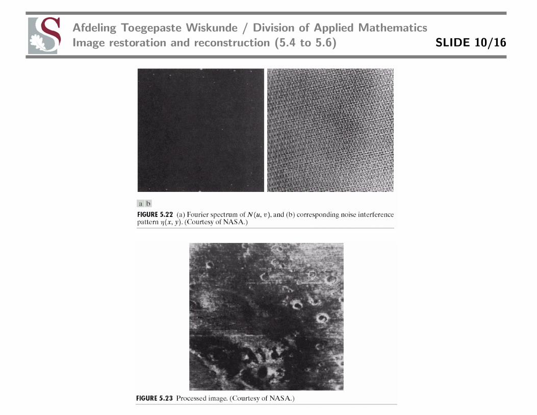
5.4.4 Optimum Notch Filtering
Starlike components in Fourier spectrum indicate more than one sinusoidalpattern
Observe G(u, v) and experiment with different notch pass filters HNP(u, v)where η(x, y) = IFT { HNP(u, v)G(u, v) }
We want to optimize a weighting or modulation function w(x, y) where
f̂ (x, y) = g(x, y)− w(x, y) η(x, y) (1)
in such a way that local variances of f̂ (x, y) is minimized

Afdeling Toegepaste Wiskunde / Division of Applied Mathematics
Image restoration and reconstruction (5.4 to 5.6) SLIDE 8/16
Consider a neighbourhood size of (2a + 1) by (2b + 1) about every point
Local variance of f̂(x, y) at (x, y):
σ2(x, y) =1
(2a + 1)(2b + 1)
a∑
s=−a
b∑
t=−b
[ f̂(x + s, y + t)− f̂(x, y) ] 2 (2)
f̂(x, y) =1
(2a+ 1)(2b+ 1)
a∑
s=−a
b∑
t=−b
f̂ (x + s, y + t)
Substitute (1) into (2):
σ2(x, y) =1
(2a + 1)(2b + 1)
a∑
s=−a
b∑
t=−b
{ [ g(x + s, y + t)
−w(x + s, y + t) η(x + s, y + t) ]
− [ g(x, y)− w(x, y) η(x, y) ]}2
Assume that w(x, y) remains constant over the neighbourhood, that is let
w(x + s, y + t) = w(x, y),then
w(x, y) η(x, y) = w(x, y) η(x, y)

Afdeling Toegepaste Wiskunde / Division of Applied Mathematics
Image restoration and reconstruction (5.4 to 5.6) SLIDE 9/16
andσ2(x, y) =
1
(2a + 1)(2b + 1)
a∑
s=−a
b∑
t=−b
{ [ g(x + s, y + t)
−w(x, y) η(x + s, y + t) ]
− [ g(x, y)− w(x, y) η(x, y) ] } 2
To minimize σ2(x, y), we solve∂ σ2(x, y)
∂ w(x, y)= 0 for w(x, y).
The result is
w(x, y) =g(x, y) η(x, y)− g(x, y) η(x, y)
η2(x, y)− [η(x, y)]2
Afdeling Toegepaste Wiskunde / Division of Applied Mathematics
Image restoration and reconstruction (5.4 to 5.6) SLIDE 10/16

Afdeling Toegepaste Wiskunde / Division of Applied Mathematics
Image restoration and reconstruction (5.4 to 5.6) SLIDE 11/16
5.5 Linear, position-invariant degradations
g(x, y) = (h ∗ f )(x, y) + η(x, y)
=
∫ ∞
−∞
∫ ∞
−∞
f(α, β) h(x− α, y − β) dα dβ + η(x, y)
G(u, v) = H(u, v) F (u, v) +N(u, v)
• Image deconvolution• Deconvolution filters
5.6 Estimating the degradation function
(1) Observation
(2) Experimentation
(3) Mathematical modelling
5.6.1 Estimation by image observation
• Given: only the degraded image• Choose subimage that contains simple structures with little noise: gs(x, y)
Afdeling Toegepaste Wiskunde / Division of Applied Mathematics
Image restoration and reconstruction (5.4 to 5.6) SLIDE 12/16
• Estimate original subimage: f̂s(x, y)
Hs(u, v) =Gs(u, v)
F̂s(u, v)
• Construct H(u, v) on a larger scale with similar “shape” as Hs(u, v)
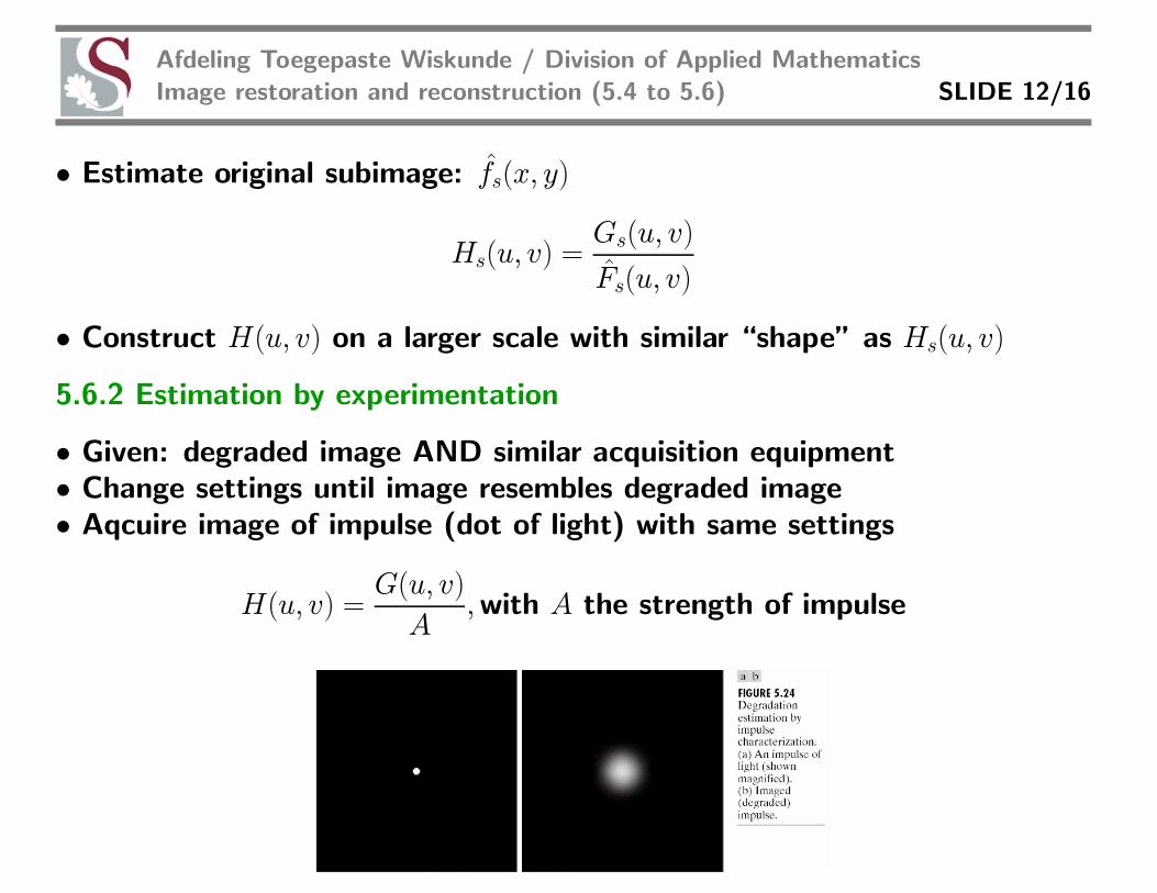
5.6.2 Estimation by experimentation
• Given: degraded image AND similar acquisition equipment• Change settings until image resembles degraded image• Aqcuire image of impulse (dot of light) with same settings
H(u, v) =G(u, v)
A,with A the strength of impulse
Afdeling Toegepaste Wiskunde / Division of Applied Mathematics
Image restoration and reconstruction (5.4 to 5.6) SLIDE 13/16
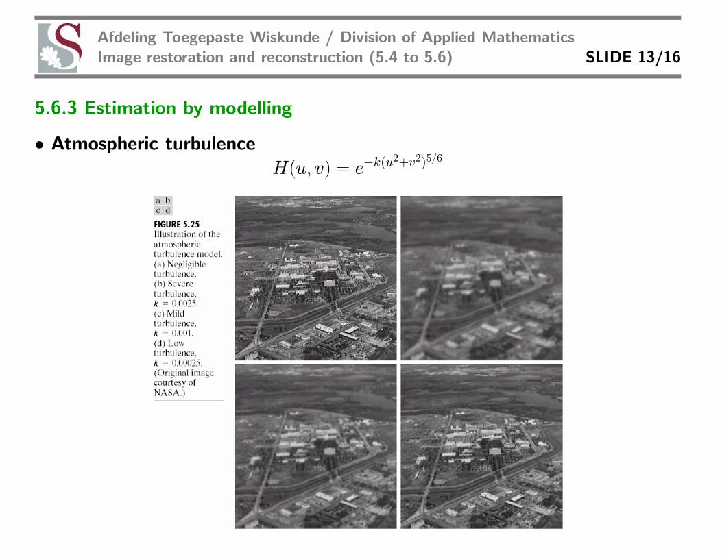
5.6.3 Estimation by modelling
• Atmospheric turbulence
H(u, v) = e−k(u2+v2)5/6

Afdeling Toegepaste Wiskunde / Division of Applied Mathematics
Image restoration and reconstruction (5.4 to 5.6) SLIDE 14/16
• Basic mathematical principles: uniform linear motion
Let T be duration of exposure, then g(x, y) =
∫ T
0
f [x− x0(t), y − y0(t) ] dt
G(u, v) =
∫ ∞
−∞
∫ ∞
−∞
g(x, y) e−2πi(ux+vy) dx dy
=
∫ ∞
−∞
∫ ∞
−∞
(∫ T
0
f [x− x0(t), y − y0(t) ] dt
)e−2πi(ux+vy) dx dy
=
∫ T
0
(∫ ∞
−∞
∫ ∞
−∞
f [x− x0(t), y − y0(t) ] e−2πi(ux+vy) dx dy
)dt
=
∫ T
0
F (u, v) e−2πi[ux0(t)+vy0(t)] dt
= F (u, v)
∫ T
0
e−2πi[ux0(t)+vy0(t)] dt
Define H(u, v) =
∫ T
0
e−2πi[ux0(t)+vy0(t)] dt so that G(u, v) = H(u, v) F (u, v)
If x0(t) and y0(t) are known, then H(u, v) is known

Afdeling Toegepaste Wiskunde / Division of Applied Mathematics
Image restoration and reconstruction (5.4 to 5.6) SLIDE 15/16
Illustration
Let x0(t) =at
Tand y0(t) = 0
Note that x0(T ) = a
H(u, v) =
∫ T
0
e−2πiux0(t) dt
=
∫ T
0
e−2πiuat/T dt
= ...
=T
πuasin(πua) e−πiua
(verify)
Note that H(u, v) = 0 if u =n
a, n ∈ Z
When x0(t) =at
Tand y0(t) =
bt
T, then
H(u, v) =T
π(ua + vb)sin[π(ua + vb)] e−πi(ua+vb)

Afdeling Toegepaste Wiskunde / Division of Applied Mathematics
Image restoration and reconstruction (5.4 to 5.6) SLIDE 16/16
Example 5.10: Image blurring due to motion
Top Related