


Languages
Pages
Legal


Growth Through Inter-sectoral Knowledge Linkages∗
Jie Cai
University of New South Wales
Nan Li
Ohio State University and IMF
January 29, 2012
Abstract
Sectors differ greatly in their degree of knowledge applicability. This paper studies the impact
of inter-sectoral knowledge linkages on aggregate innovation and growth. We develop a multi-
sector model in which exogenous inter-sectoral knowledge linkages affect firms’ sector entry/exit
and R&D decisions. In the presence of barriers to diversity, the model generates sequential
sectoral entry, which helps to explain firms’ patenting locations in the technology space, the
empirical relationship between a sector’s knowledge applicability and other variables including
R&D intensity, the number of firms and the firm size distribution in that sector. We construct
an inter-sectoral knowledge diffusion matrix and simulate the model. A main finding is that
barriers to diversity significantly reduce technological progress beyond what is expected from
previous studies; in particular they block the knowledge circulation in the technology space and
prevent firms from fully internalizing spillovers from sectors with high knowledge applicability
and investing in research in these sectors.
Keywords: economic growth; technological change; cross-sector technology spillovers; R&D;
multiple sectors; resource allocation
JEL Classification: O30, O31, O33, O41, L16.
∗This paper is a substantially revised version from the previously circulated draft “Knowledge Linkages andFirm Innovations”. We would like to thank Paul Beaudry, Bill Dupor, Chris Edmond, Sotirios Georganas, JoeKaboski, Aubhik Khan, Amartya Lahiri, Roberto Samiengo, Mark Wright and seminar participants at the Econo-metric Society Winter Meeting, ASSA-2012, University of Melbourne, Ohio State University, the UNSW-Universityof Sydney joint macro seminar, Reserve Bank of Australia, Chinese University of Hong Kong and the IMF institutefor helpful comments. Correspondence: Jie April Cai, Department of Economics, University of New South Wales,[email protected]; Nan Li, Department of Economics, The Ohio State University, [email protected].
1

1 Introduction
Innovation hardly ever takes place in isolation: technologies depend upon one another. Yet, they
vary substantially in their degree of applicability. Some innovations, such as the electric motor,
create general purpose knowledge that can be easily adapted to design new products in a vast
range of sectors. Other inventions, such as the space pen, introduce technologies that are limited
in their scope of application. The interconnections between different technologies and the stark
contrast in the way new technologies affect future innovation have long been recognized by economic
historians.1 The majority of theoretical work on technological change and endogenous growth,
however, studies single-sector models or multiple-sector models but treating innovations in different
technologies as isolated from each other and equally influential.2
The transmission of technological change from one sector of the economy to another through
knowledge spillovers has important implications for our understanding of the innovation process
in an economy. Specifically, empirical evidence presented in this paper suggests that intersectoral
knowledge spillovers are heterogeneous and highly skewed : a small number of technologies are
responsible for fostering disproportionately many subsequent innovations in the economy.3 Thus,
the allocation of R&D across different technologies and government policy directed at stimulating
innovations in certain sectors can have far reaching consequences for economic growth.
The main contributions of this paper are threefold. The first is to develop a multi-sector general
equilibrium model that can be used to study how intersectoral knowledge linkages affect growth.4
Our model extends the previous literature on firm innovation and growth (especially, Grossman
and Helpman, 1991a; Klette and Kortum, 2004) to a multi-sector environment, where each firm
makes sector entry, exit and R&D decisions. Empirically, the majority of new technologies are
developed by multi-sector firms which are able to internalize intersectoral knowledge spillovers.5
1David (1991), Rosenberg (1982), Landes (1969), for example, emphasize the dramatic impact on growth playedby key technologies, such as the steam engine, the factory system and semiconductor.
2For notable exceptions, see Akcigit and Kerr (2010, 2011), which will be discussed below.3Using firm-level R&D investment data in five high-tech industries, Bernstein and Nadiri (1988) finds that knowl-
edge spillovers largely vary across sectors and are highly significant. Wieser (2005), in his survey paper, claims thatspillovers between sectors are more important than those within sectors, when considering both the social and privatereturn of R&D.
4Throughout the paper, we use the terms technologies and sectors interchangeably. In the model, one patent orone new innovation is necessarily turned into a product in that sector. Although distinguishing a firm’s position intechnology space and product space is interesting for certain issues, it is not the interest of this paper and has beenexplored in Bloom et al. (2010).
5More than 42% of patenting firms innovate in more than one technological fields and these firms account forthe majority of innovation in the economy. Related to this observation, in the firm-product data, 41% of U.S.manufacturing firms which operate multiple product lines account for 91% of total sales (Bernard, Redding andSchott, 2006). Therefore, understanding how firms expand their technology and product range sheds light on both
2

Such a model, thus, also helps us understand how firms decide on what kind of technologies (e.g.
general purpose versus limited scope) to develop, which sectors to apply its technologies in and
grow its business. The model is motivated by and is able to reproduce the empirical observations
documented in Section 2. Second, we use this framework to clarify and highlight key factors that
may affect how intersectoral knowledge linkages contribute to growth. Most prominently, we show
that barriers to diversity may significantly reduce equilibrium technological progress by preventing
firms from internalizing knowledge spillovers across sectors and blocking the knowledge circulation
in the technology space. Our model also implies that when firms face volatile idiosyncratic shocks to
barriers to diversity, the ‘fundamental’ factor—sectoral knowledge linkages—plays a less important
role in directing the allocation of firm’s R&D across sectors, and the inefficient allocation of research
leads to substantial reduction in innovation and growth. Third, we calibrate and simulate the model
to (a) assess the performance of the model, and (b) quantify the extent to which changes in various
key factors may affect the aggregate technological and economic growth.
In our model, new products are invented by conducting R&D to adapt (both internal and exter-
nal) existing knowledge in various sectors. The productivity of this activity depends on the ‘deep’
fundamental knowledge linkages between sectors. Not only do GPTs enhance future innovations in
the current sector, they also increase the innovation productivity of R&D in downstream sectors
and contribute to a sequence of innovations in various sectors—exhibiting ‘innovational comple-
mentarities’. Consistent with this observation, in the model the equilibrium value associated with
the introduction of a new innovation is not confined to its own future profit gains; rather, it also
depends on the application value of this new technology in all sectors.
For any given sector a firm intends to enter or continue operating in, a period-by-period fixed
cost is required. These fixed costs, acting as barriers to diversity, make research in multiples sectors
a self-selection process: a firm develops new products in sectors where it can most efficiently utilize
its existing range of technologies. Although the high application value of the GPTs attract firms to
enter there first and invest intensively in R&D, the model suggests that a counteracting force is at
play: the fierce competition in these sectors. Firms would only conduct research and operate in a
sector if the expected value of adapting its accumulated knowledge capital in related sectors is large
enough to cover the fixed cost of research.6 Therefore, given its current position in the technology
technological progress and aggregate production, although this paper focuses on technical advances.6Firms in the model are subject to idiosyncratic sectoral innovation shocks, which is i.i.d over time and across
firms. Thus, a firm exits a specific sector if it experiences a range of negative shocks such that the expected payoff ofoperating in that sector cannot cover the fixed cost. As will be shown in Section 4.1, these idiosyncratic shocks alsohelp to ensure a stationary Pareto firm size distribution.
3

space, smaller (or younger) firms with less knowledge scope tend to self-select into technologies with
higher applicability—what we call ‘central sectors’ in the technology space—whereas firms with
large knowledge stock in multiple sectors tend to expand into technologies with lower applicability
but allowing them to have larger market shares—what we call ‘peripheral sectors’. Consistent with
the empirical observations documented in Section 2.3, firms conducting research in multiple areas
are better at internalizing intersectoral knowledge spillovers, thus have stronger incentives to invest
in research in central GPTs. The tradeoff between innovational applicability and product market
competition—which is at the heart of the R&D resource allocation mechanism in the economy—
leads to a stationary firm distribution across sectors and a stationary (normalized) sector size
distribution on the balanced growth path.
At the aggregate, our model predicts that equilibrium R&D intensity is higher in sectors with
larger knowledge application value. While this value is not directly observable, the model suggests
that it increases with its innovational ‘applicability’, the ability to foster technical advances in
a wide variety of sectors. Using U.S. patent citation data, in Section 2.1 we construct such a
measure that quantifies the applicability or generality of purpose of different types of technology.7
Employing U.S. Compustat firm R&D data, we find that R&D intensity in sectors with highly
applicable knowledge is indeed larger.8
Barriers to diversity lower economywide innovation through two related but distinct mecha-
nisms. First, in the presence of these barriers, only a small fraction of firms can afford a sequence
of fixed costs and reach the periphery of the technology space; most firms are excluded from cross-
sector knowledge applications between central sectors and peripheral sectors. Higher barriers, thus,
directly block the knowledge circulation in the entire technology space and impose a first-order neg-
ative effect on technical advances. Second and more subtly, when these barriers rise, central sectors
become relatively more competitive compared to peripheral sectors, due to the more pervasive use
of their technology in future innovations. The increased competition reduces the potential gains
from new products, discouraging further research in these areas. The equilibrium consequence is
a disproportionate fall of innovation in central sectors, the effect of which propagates pervasively
7We intentionally choose to concentrate on the implications of ‘deep’ , time-invariant characteristics of technologicallinkages on firm’s innovation. Thus, we use patent citation data over 30 years (1976-2006) to form the knowledge flownetwork. The relationships of knowledge complementarity make it difficult to evaluate the contribution of any singleinnovation to the whole technology space. To handle this issue, we apply Kleinberg’s (1998) iterative algorithm—which is proved to be the most efficient at extracting information from a linked environment—to the technologynetwork, and develop a sector specific measure of knowledge applicability.
8Sectoral R&D intensity is calculated as total R&D expenditure at the sector level divided by total sales, byaggregating firm-level data up to the sector level. The correlation between sectoral R&D intensity and applicabilityequals 65 percent and is highly significant.
4

throughout the economy and causes a lower aggregate innovation rate.9
Firms entering multiple sectors sequentially—that is, firms typically start from central sectors
and slowly venture into periphery after accumulating enough private knowledge in various sectors—
is a general pattern in the model, however not all firms follow the same sequence. This is because,
first, innovation is highly uncertain; second and more interestingly, in the absence of strict imple-
mentation or clarity of the regulatory framework, firms may face relationship-based idiosyncratic
barriers to entry. Therefore, firms may choose to orient their research towards directions that are
not dictated by the common fundamental factors—the knowledge applicability. An increased vari-
ance of the idiosyncratic fixed costs injects more noise in firms’ sector selection decisions and makes
this decision process more random. Firms with sufficient background knowledge may not be able to
conduct research in many sectors anymore, and firms with insufficient background knowledge may
enter many sectors but cannot innovate much. The inefficient sorting of firms in different sectors
leads to large reduction in aggregate innovation.10
In any given sector, existing firms innovate, expanding their size as they create new varieties,
and exit after experiencing a sequence of negative innovation shocks or a sequence of high draws
of fixed costs. In addition, new firms enter if they have accumulated enough knowledge capital in
related sectors. This process endogenously generates a distribution of firm size in each sector (and
in the whole economy), which converges to a Pareto distribution in the upper tail.
We estimate the model using U.S. patent data and firm R&D data from the Compustat dataset
and simulate a model economy with a large number of multi-sector multi-product firms with various
ranges of technologies.11 We test the implications of the model and assess the growth effects of
sectoral fixed costs. We find that a single source of heterogeneity across sectors—intersectoral
knowledge linkages—can account for most observed heterogeneity across sectors, including the
number of firms in different sectors, the distribution of firms by the number of sectors, R&D
expenditure shares and the shapes of firm size distribution.
We then use the quantified model to evaluate the impact of increasing the mean and the standard
9The economic channel through which entry costs decrease growth in this paper is very different from the onesstressed in the previous literature. For example, entry costs discourage small but innovative entrepreneurs from entryand keep existing establishment inefficiently large in Boedo and Mukoyama (2009), or they distort the allocation oftalent across sectors as in Buera, Kaboski and Shin (2011). In Barseghyan and DiCecio (2010), higher entry costsreduce productivity of the marginal entrant through a general equilibrium effect on wage.
10In an environment where agents in charge of licensing can interpret the regulation policy according to their ownunderstanding, there is scope for corruption and rent seeking. The result above suggests that policy specificationsshould be as clear as possible, so that the implementer has little discretion.
11U.S. Patent and Trademark Office (USPTO) data contained patent information across 428 technology classes,which can be mapped into 42 SIC 2-4digit industries. For simulation, we estimate the knowledge diffusion matrix for42 sectors, as it is more feasible technically.
5

deviation of idiosyncratic sectoral fixed costs. We show by simulation that the effect is strong;
doubling the size of the average fixed costs reduces the aggregate innovation rate from 11% to 6.6%
and the growth rate from 2% to 1.29%. When increasing the standard deviation of the fixed costs
from 0.5 to 5, the innovation rate decreases substantially to 1.13% and the growth rate to 0.26%.
Related Literature Most endogenous growth models (e.g. Romer, 1986, 1990; Lucas, 1988;
Segerstrom and Dinopoulos, 1990; Aghion and Howitt, 1992; Grossman and Helpman, 1991a,
1991b and Jones, 1995) have in the past considered a single type of technological change. Similarly,
the majority of recent theoretical work on innovation and firm dynamics (e.g., Klette and Kortum,
2004; Luttmer, 2007 and Atkeson and Burstein, 2010) assumes that a firm’s innovation applies
to a product or a sector that is randomly drawn from a pool. There are no explicit interactions
between different sectors or distinctions between innovations with different degrees of generality,
and hence, no room to discuss the relationship between R&D investment allocation across sectors
and economic growth.
Work along the line of distinguishing different types of research and their impact is currently
being pursued in a number of papers. In particular, Akcigit and Kerr (2010) study how explo-
ration versus exploitation innovations affect growth; similarly to this notion, Acemoglu and Cao
(2010) consider incremental R&D engaged by incumbents and radical R&D undertaken by potential
entrants.12 Similar to Acemoglu and Cao, our paper also allows for simultaneous innovations by
continuing firms and entrants; however, the different technological fields in which large versus small
firms or incumbent versus entrants innovate in our model is an endogenous equilibrium outcome.
More closely related, Akcigit, Hanley and Serrano-Velarde (2011) distinguish between basic research
and applied research to analyze the impact of the appropriability problem on firms’ incentives to
conduct basic research and its consequence on growth. We consider the technological interdepen-
dence across all sectors instead of two distinct types of research as in their paper. Bresnahan and
Trajtenberg (1995) study using a partial equilibrium analysis how market microstructure affects
the incentives to innovate in a single source sector that they regard as critical in fostering technical
progress (GPT) and several application sectors, whereas we consider all sectors and their bilateral
technology interconnections.
12Ngai and Samaniego (2010), in their working paper version, suggest including cross-industry spillovers into theirmodel which identifies factors that account for endogenous differences in research activities and productivity growthacross sectors. However, they abstract from this because they find that citations are dominated by within-industrycitations, speculating that cross-industry spillovers are small. We show in this paper that, although small in absolutequantity, it is large enough to have significant implications on growth.
6

On the empirical front, most studies of technology diffusion in the past have focused on spillovers
between firms or across geographic regions.13 For example, also using firm patenting information,
Bloom, Schankerman and Van Reenen (2010) develop a technological proximity index between
patenting firms and distinguish it from product closeness between firms. Different from our focus—
spillovers across sectors, they investigate the positive (cross-firm) technology spillover effects versus
the negative product market rivalry effects of R&D on firm’s performance.
Our work also contributes to the earlier literature in development economics that emphasizes
the role of sectoral linkages and complementarity in explaining growth.14 Prior work in this area
typically focuses on material input-output relationships between sectors—as in Jones (2010a), and
export-based measures of sectoral relatedness—as in Hidalgo, Klinger and Hausmann (2007).15
This paper focuses on linkages dictated by their knowledge content, which is more suitable for
understanding the mechanics of technological innovation. We also develop sector-specific measure
of knowledge applicability that captures its overall importance in the whole technology space. Our
paper is also related to the expanding literature on misallocation and economic growth.16 Jones
(2010b) suggests that misallocation effects can be amplified through the input-output structure of
the economy. In out context of knowledge spillovers, the misallocation of research hurts growth
mainly because highly applicable knowledge is underdeveloped and not sufficiently utilized by
innovating firms.
2 Empirical Underpinning
In this section, we first document empirical observations that motivate our model using patent ci-
tations, firm patenting and R&D information. Merging firm patent data and U.S. Census firm-level
data, Balasubramanian and Sivadasan (2011) find that although only 5.5% of all manufacturing
firms engage in patenting activity, they play an important role in the aggregate production, ac-
counting for about 60% of value added.
Our main datasource is the 2006 edition U.S. Patent and Trade Office (USPTO) data from
1976 to 2006.17 Patent applications serve as proxies of firm’s innovative output and their citations
13See Jaffe (1986, 1988), Branstetter (2001), Bottazi and Peri (2007), Belenzon and Schankerman (2011).14See Leontief (1936), Hirschman (1958).15Other research studies the role of input-output relationship in understanding sectoral co-movements and the
transmission of shocks over the business cycle, such as Lucas (1981), Long and Plosser (1993), Basu (1995), Horvath(1998), Conley and Dupor (2003), Carvalho (2009).
16For example, Ciccone (2002), Restuccia and Rogerson (2008), Hsieh and Klenow (2009).17See Hall, Jaffe and Trajtenberg (2001) for detailed description of the data.
7

are used to trace the direction and intensity of knowledge flows within and across technological
classes.18 Each patent corresponds to one of the 428 3-digit United States Patent Classification
System (USPCS) technological field (NClass). We summarize citations made to (and from) patents
that belong to the same technological class to form the inter-sectoral knowledge spillover network.
Another source of data is from U.S. Compustat 1970-2000 which includes firm level R&D expendi-
ture and firm performance data. We use this information to construct sector-level R&D intensity.
Details regarding the data and construction of various measures are provided in Appendix A.
2.1 Heterogeneous Sectoral Knowledge Applicability
We use sectoral patent citation data to estimate the knowledge input-output matrix. Each element
of the knowledge diffusion matrix measures the relative contribution of the source sector’s knowledge
in a receiving sector’s innovation activity. We proxy this knowledge linkage by the fraction of
(outward) citations (OC) made to sector j by sector i, OCij/∑
j OCij . Since sectors with more
patents tend to be cited more frequently, we handle this by normalizing the citation percentage by
the relative importance of sector j, measured by the share of (inward) citations received by j in
total citations, ICj/∑
j ICj . Formally,
Aij =OCij∑j OC
ij/
ICj∑j IC
j(1)
This matrix is highly asymmetric: Aij 6= Aji.19
The pairwise measure A we develop captures the ‘application intensity’ between any two sectors
but cannot be directly used to rank the overall application value of different technologies to the
entire technology space. One simple method is to aggregate Aij over all the citing sectors j. The
problem with this method is that it assumes that all links indicated by a citation are equally
strong. However, when two sectors receive the same number of citations, it is desirable to rank
the sector that receives citations from more ‘important’ sectors higher. To handle this issue, we
apply Kleinberg’s (1998) algorithm to the cross-sector patent citation network and construct a
measure quantifying the applicability of each technology, called in the original paper ‘authority
weight’ (denoted by ai in sector i). Kleinberg’s algorithm—which has proved to be most efficient in
extracting information from highly linked environments—is a fixed point iteration which generates
18We only consider patents by domestic and foreign non-government institutions.19It is important to note that this is different from the normal technology closeness measure—as in Jaffe (1986)
and Bloom et al. (2010), in which the distance between any two technologies is independent from the direction.
8

Figure I: Distribution of Knowledge Applicabilities Across Sectors
010
2030
40Pe
rcen
t
0 .005 .01 .015Applicability (Truncated 95th Percentile)
Notes: The applicability measure is constructed by applying Kleinberg’s algorithm to the cross-sector patent citation
network (NBER Patent Dataset, 1976-2002) (see details for the algorithm n Appendix A.2).
two inter-dependent indices: authority weight and hub weight. Intuitively, the technology with
high authority weight generates large knowledge flows to sectors with highly ranked hub weights,
and the technology with high hub weight largely utilizes knowledge flows from sectors with highly
ranked authority weights. Therefore, this measure makes use of knowledge flow information from
the entire technology network. Appendix A.2 provides the detailed calculation of this measure.
Figure I shows the highly skewed distribution of our measure of knowledge applicability across
sectors, with a small number of sectors acting as the knowledge ‘authority’ in the technology space.
Alternatively, and as a robustness check for our results, we use a pairwise technology distance
measure which is based on the shortest path between any two sectors in the technology network
(see Appendix for detailed explanations). The sector specific applicability measure is then the
weighted average of distances to all other sectors, using the inverse of the number of citations made
by another sector as weights.
2.2 R&D Intensity and Technology Applicability Across Sectors
R&D intensity—defined as R&D expenditure divided by sales—differs greatly across sectors. Figure
2.2 shows there is a strong positive relationship between the R&D intensity in a sector and the
applicability of its technology. In later sections of the paper, we show that the sectoral R&D
intensity in our model is positively proportional to the market value of the sector’s knowledge
9

capital, which in turn is mostly determined by the application value of the knowledge.
Figure II: Sectoral R&D Intensity Significantly Increases with Its Applicability
log(R&D/Sales) = 0.653 + 0.663 log(a)
(0.161)***
−6
−4
−2
02
Avera
ge R
&D
Inte
nsity (
1970−
2000, in
log)
−6 −4 −2 0Applicability
Notes: R&D intensity is the average ratio of R&D expenditures to sales among firms in Compustat over the period
1970-2000. The applicability measure is constructed by applying Kleinburg’s algorithm to the cross-sector patent
citation network (NBER Patent Dataset, 1976-2002) (see details for the algorithm n Appendix A.2). The solid line
represents the fitted values. The brackets under the regression coefficient estimates shows the standard errors for the
estimates.
2.3 Firm Patent Allocation, Patent Stock and Multi-Technology Patenting
Each firm is characterized by a vector of patents in all technological classes. We use the share
of (accumulated) patents per firm in each technology class in 2000 as our measure of the firm’s
technological activity and also knowledge distribution, defining the vector Tf = (T if , T2f , ..., T
428f ),
where T if is the share of patent stocks of firm f in technology class i. In order to summarize a firm’s
patent allocation in the technology space, we construct a measure of a multi-sector firm’s overall
technology applicability, TAf , as the patent-stock-weighted geometric mean of the applicability of
individual technology i, ai. That is, TAf =∏i(a
i)Tif . To measure multi-technology patenting, we
count the number of distinct technology classes a firm has patented in. In the data, 42% of the
patenting firms innovate in more than one technology field over the period 1976 to 2000, and larger
firms innovate in more areas—e.g. firms with a patent stock that lies in the top quartile on average
acquire patents in 146 technology classes.
The left panel in Figure 2.3 plots the technology allocation measure of a firm, TAf , against its
patent stock, distinguishing sectors a firm just entered in 2000 (the downward sloping fitted line)
10

from sectors in which the firm has previously patented (the outward sloping fitted line).20 The
right panel of Figure 2.3 plots the same technology allocation measure against the total number of
technology classes where the firm innovates in. Firm patent stocks and the number of technology
classes are each divided into 30 bins. Each figure presents the variable of interest according to the
bin.
Figure III: Firm’s Technology Applicability, Patent Stock and Multi-Technology Patenting
All Sectors Firms Have Patented In
New Sectors Firms Enter
−7.8
−7.2
−6.6
−6
−5.4
Applic
abili
ty o
f F
irm
’s T
echnolo
gy P
ort
folio
(in
log)
2 4 6 8 10Patent Stock (in log)
−6.7
−6.2
−5.7
−5.2
Applic
abili
ty o
f F
irm
’s T
echnolo
gy P
ort
folio
(in
log)
0 1 2 3 4Number of Technology Classes (in log)
Notes: Y-axis measures the (weighted) average applicability of the firm’s patent portfolio, log TAf . Firms are divided
into 30 bins according to their patent stocks (left panel) or their number of technology classes (right panel). Each
observation corresponds to an average firm in the size bin. Datasource: NBER Patent Data, 2006 edition.
Two observations stand out. First, the left panel illustrates the scale dependence in firms’ patent
allocation and entry pattern.21 A firm with a higher patent stock tends to allocate more patents in
technologies with high applicability; however, this observation is sharply reversed when focusing on
the newly entered patent classes. The new sectors that firms with more patents enter tend to be the
ones with lower applicability. Second, independent of the size of the firm’s patent stock, the new
sectors entered by a given firm tend to be lower in applicability relative to the existing sectors except
20A sector is new to a firm if the firm has not innovated in that sector before. The full dataset expands from 1901to 2006, thus, provides a good sample for identifying new sectors.
21We approximate firm size by a firm’s patent stock in all sectors. We can use name-matching procedures providedby Hall, et al. (2005) to link the NBER patent data to Compustat firm data; however, only 15% of the patentingfirms are in Compustat. Based on this limited information, we find that the patent stock is positively correlated withstandard measures of firm size (correlation coefficient is 0.6): sales and employment.
11

for the very small firms (i.e. the observations that identify new sectors lie below the observations
of all sectors). Third, as manifested in the right panel, the higher average applicability of the firm’s
technologies is also associated with its multi-technology patenting.22 These observations also hold
using the alternative distance-based measure of knowledge applicability.
Appendix A.4 provides further evidence on the relationship between a firm’s patent allocation,
patent stock and multi-technology patenting using a fixed-effect panel regression. Table A.1 shows
that a firm with a higher patent stock allocates significantly more innovative output (patent)
in highly applicable sectors and firms with more applicable technology acquire patents in more
technology classes. We have also investigated and confirmed the robustness of these relationships
at a different level of disaggregation: at 42 industries level or the IPC classification based 800
sectors.
3 Model
Our model focuses on firms’ innovation behavior and regards product innovation as a process of
generating new varieties in different sectors. Thus, the model is built on the tradition of variety
expanding models (e.g., Romer 1990; Grossman and Helpman 1991; Jones 1995). Recently, Bala-
subramanian and Sivadasan (2011) provide strong empirical evidence showing that firm patenting
is associated with firm growth through the introduction of new products.23 The strong link be-
tween patenting and firm scope also suggests that it may be important to consider firm scope as
the source of heterogeneity across innovating firms.24 Our interpretation of innovation and firm
heterogeneity in the model are both consistent with these empirical observations.
Compared to the standard endogenous growth models, this model has three distinct features.
First, the model features a multi-sector environment: a firm conducting R&D in one specific sector
may apply knowledge accumulated in all related sectors. In the patent data, more than 42% firms
have patents in more than one technology categories and 44% of patent citations are inter-sector
citations.25 These observations highlight the important role of cross-sector knowledge spillovers
in individual firms’ innovation behavior. Second, in the model, for any sector a firm intends to
22This is consistent with Nelsons’ hypothesis (1959) and findings in Akcigit et al. (2011)—a broader technologicalbase positively correlates with higher investment into basic research relative to applied research.
23Earlier evidence cited by Scherer (1980) also shows that firms allocate 87% of their research outlays to productimprovement and developing new products and the rest to developing new processes.
24Also in Klette and Kortum (2004), Bernard Redding and Schott (2006b) and Nocke and Yeaple (2006), firms areheterogeneous in terms of their product scopes.
25This is based on 428 technology classes for the period 1976-2006. The percentage becomes higher when usingmore disaggregated classifications
12

conduct research in, it has to pay a period-by-period fixed cost. These sectoral fixed costs act
as barriers to diversity, preventing firms from developing products in all sectors. However, fixed
costs generate an advantage for firms with large knowledge scope in their innovation activity and
allow them to enjoy high market shares in less populated peripheral sectors. Third, both incumbent
firms and potential entrants innovate, and there is a public knowledge pool that all firms can access.
The public knowledge in the model allows a completely newborn firm to enter the economy in the
presence of the fixed costs. Access to public knowledge also prevents firms from getting too small,
which helps to ensure a stationary firm size distribution. Various case studies (Abernathy, 1980;
Lieberman, 1984 and Scherer, 1984) provide evidence showing that innovations by existing firms
are as important as (if not less than) entering firms in the same line of business.26 In addition,
in patent data, 85% of citations are given to patents owned by other institutions, suggesting that
public information and imitation are important knowledge sources for individual R&D conducting
firms.
3.1 Demand
The economy is populated by a unit measure of identical infinitely-lived households. Households
do not value leisure and order their preferences over a life-time stream of consumption {Ct} of the
single final good according to
U =
∞∑t=0
βtC1−ηt − 1
1− η(2)
where β is the discount factor and η is the risk-aversion coefficient. A typical household inelastically
supplies a fixed unit of labor, L, which the household can allocate to work as production workers,
researchers or workers in the licensing industry. Households have access to a one-period risk-free
bond with interest rate rt and in zero aggregate supply. Maximizing their life-time utility subject
to an intertemporal budget constraint requires that consumption evolve according to
β(Ct+1
Ct)−η
PtPt+1
(1 + rt) = 1, (3)
There are three types of goods in the economy: a final consumption good, sectoral goods
and sectoral-differentiated varieties (or brands). To concentrate on heterogeneity in knowledge
spillovers across sectors, we abstract from other possible sources of sectoral heterogeneities, such as
26Innovations by existing firms have also been incorporated into models in other studies, such as Luttmer (2007),Atkeson and Burtein (2010) and Acemoglu and Cao (2010). Our modeling strategy for the interaction betweenentrants and incumbents is similar to Luttmer in that there are knowledge spillovers across firms.
13

expenditure shares, elasticities of substitution between varieties and cross-firm knowledge spillover
intensities. The final good is produced by combining quantities of K different sectoral intermediate
goods {Qit} according to a Cobb-Douglas production function
log Yt =K∑i=1
si log(Qit), (4)
where, si = 1/K captures the share of each sector in production of the final good. Without physical
capital in the model, the final good is only used for consumption: Ct = Yt.
At any moment, each sector contains a set of varieties that were invented before time t. In
particular, we represent the set of varieties in sector i available on the market by the interval
[0, nit]. Sector i good is aggregated over these nit number (measure) of differentiated goods that are
produced by individual monopolistically competitive firms
Qit =
[∫ nit
0
(xik,t)σ−1
σ dk
] σσ−1
, i = 1, 2, ...,K, (5)
where xik,t is the consumption of variety k in sector i and σ > 1 is the elasticity of substitution
between differentiated goods of the same sector i. Each new variety substitutes imperfectly for
existing ones, and the firm which develops it exploits limited monopoly power in the product
market. In linking the model to the data, we interpret our sector as corresponding to different
technology classes in the patent data, while varieties within a sector map into patents.
The associated final good price is Pt = B∏Ki (P it )
si , where B is some constant consistent with
the Cobb-Douglas specification in (4) and sectoral price index, P it is given by
P it =
[∫ nit
0p1−σk,t dk
] 11−σ
. (6)
These aggregates can then be used to derive the optimal consumption for sector i and for individual
variety k in sector i using
Qit =siPtYtP it
, (7)
xik,t =
(pik,tP it
)−σQit. (8)
14

3.2 Goods Production
Firms undertake two distinct activities: they create blueprints for new varieties of differentiated
products, and they manufacture the products that have been invented previously. The firm who
invents a new variety is the sole supplier of that variety. As the focus is upon firms’ innovation
activities, the production side of the model is kept as simple as possible. We assume that each
differentiated good is manufactured according to a common technology: to produce one unit of any
variety requires one unit of labor, yift = lift, ∀i, f .
Without heterogeneity in supply and demand, all varieties in the same sector are completely
symmetric: they are charged at the same price and are sold in the same quantity. The firm
producing variety k in sector i faces a residual demand curve with constant elasticity σ specified in
(8).27 Wage is normalized to one. This yields a constant pricing rule pik,t = σσ−1 , ∀ k and t. Thus
the sectoral price, P it = σσ−1(nit)
11−σ , decreases with the total number of varieties in that sector as
σ > 1.
Combining the pricing rules with (6) and (8), we derive the total profit in the product market
in sector i (aggregated over all varieties produced by different firms) as a constant share of nominal
GDP, PtYt :
πit =
∫ nit
0
pik,txik,t
σdk =
siPtYtσ
. (9)
The total demand for production labor in sector i is
Lpit =
∫ ni
0xik,tdk =
σ − 1
σsiPtYt. (10)
3.3 Knowledge Production
There is a continuum of firms, each develops new varieties and produces in multiple sectors. A firm
at time t is defined by a vector of its differentiated products in all sectors,
zf,t = (z1f,t, z
2f,t, ..., z
Kf,t),
where zif,t ≥ 0 is the number of differentiated sector-i goods produced by firm f at time t. To add
new varieties to its set, a firm devotes a given amount of labor to R&D. Since only the firm who
invents the variety has the right to manufacture it, zf,t also defines the distribution of the firm’s
27To make the analysis more tractable, we follow Hopenhayn (1992) and Klette and Kortum (2004) by assumingthat each firm is relatively small compared to the entire sector.
15

private knowledge capital across sectors.
Let Sf,t denote the set of sectors in which firm f produces at time t, i.e. Sf,t = {i: s.t.
zif,t > 0} and F i,t = {f : s.t. zif,t > 0} denote the set of firms that produce in sector i. Then
nit =∫f∈Fi,t zf,tdf.
Consider a firm f in sector i with a stock zif,t of private knowledge at time t. For simplicity,
we assume knowledge never depreciates. The sectoral knowledge of firm f , thus, accumulates over
time according to the function
zif,t+1 = zif,t + ∆zif,t, (11)
New sectoral knowledge (or new varieties), ∆zif,t, is generated based on a innovation production
function, using the firm’s R&D input and accessible knowledge stock in all sectors and is subject
to idiosyncratic innovation shocks. Since knowledge spillovers (both within and across sectors)
are heterogenous, we decompose firm’s sectoral R&D investment according to its source sector.
One interpretation is that firms have to devote a certain amount of time digesting and adopting
knowledge in one sector to apply it to another. For clarity, we introduce the following notation:
the second index, j, stands for the sector that the firm is adopting knowledge from—the source
sector, while the first index, i, stands for the sector that the firm is applying the knowledge to—
the application (or target) sector.28 Thus, Rijf denotes firm’s R&D input when utilizing sector j’s
knowledge to generate new knowledge (invent new goods) in sector i.
The new sector-i knowledge created by firm f summarizes innovation output in different R&D
activities, each utilizing a different type of source knowledge. One of the central notions of our paper
is that the productivity of total innovation inputs depends on the asymmetric knowledge input-
output matrix, {Aij}i,j=1,..,K , which is taken as exogenous by firms.29 Specifically, new knowledge
is produced based on a Cobb-Douglas combination of innovation productivity, the firm’s current
R&D investment and its knowledge capital:
∆zif,t =K∑j=1
[Aij(zitR
ijf,t
)α (T jf,t
)1−α+ zif,tε
ijf,t
](12)
where α is the share of R&D in the innovation production. We explain the elements of this
28When i = j, it captures the within-sector knowledge spillovers.29It might be true that technologies advance over time and the interaction between one another evolves, forming a
dynamic network instead of a static one. Also, these relationships of complementarity may be hard to predict and notnecessarily visible or well understood by innovators. Here, we intentionally choose to concentrate on the implicationsof very ‘deep’ , time-invariant characteristics of technological linkages on firm’s innovation and leave the study ofdynamic knowledge network formation to future work, as we clearly view it as a necessary first step.
16

production function in turn as below.
First, similar to Klette and Kortum (2004), we assume that innovation production function in
each sector is homogenous of degree one in effective R&D, ziRijf , and knowledge capital, T if .30 This
constant elasticity of substitution function neutralizes the effect of firm size on the innovation pro-
cess. In addition, the researchers’ efficiency is assumed to be proportional to the average knowledge
per firm in the innovating sector, zit, thus the effective R&D is given by zitRif,t. This assumption
keeps the total number of R&D workers constant in the stationary equilibrium while the number of
goods grow. Also, as will be explained later in Section 4.3, it helps to remove the ‘scale effect’ from
the model—that is, the endogenous growth rate of the economy is independent of the population
size.
Second, in the process of innovation, firms draw upon both the internal sources and the external
sources for expansion (such as learning or imitating from its competitors).31 Hence, firms innovate
in sector i by utilizing all existing knowledge at its disposal: its private knowledge stock from every
sector j ∈ Sf,t, and public knowledge from all sectors. Here, we assume the size of the public
knowledge pool is proportional to the average knowledge stock per firm in sector j, zjt , for the
following reasons. When learning from competitors is costly, each firm is too small to access all
stock of knowledge in the whole sector. When firms randomly meet and imitate a limited number
of peers, the average knowledge capital per firm is a better proxy for the size of public knowledge
than the total knowledge stock in that sector.32 Overall, the accessible pool of sector j knowledge
for firm f is given by T jf,t = zjf,t + θzjt , where θ governs the importance of the public knowledge
relative to the in-house knowledge.
Third, innovation by its nature includes the discovery of the unknown; therefore, the success of
a research project can be uncertain. We assume that firm innovation success rate,∆zif,tzif,t
, is subject
to an innovation shock εijf,t ∼ G(ε) that is identical and independently distributed across firm,
sector-pairs and time.33 Firms know the distribution of εijf,t but not their actual realizations before
30Different from our paper, Klette and Kortum (2004) specifies the innovation arrival rate as a function of thefirm’s R&D and knowledge capital.
31Although we are not modeling imitation formally here, many empirical studies have shown that a large percentageof the patented innovations were imitated quickly by other firms and imitation externalities are important for newentrants and the expansion of incumbents.
32As shown later, this assumption also helps to ensure that the sectoral growth rate is independent of the numberof firms and the total population in the general equilibrium.
33εijf,t is zero mean random variables bounded from below, such that the innovation rate is always positive. Weassume that firms do not innovate on its existing variety, but other firms can and when they succeed, the exactvarieties created by other firms would replace the existing one, resembling creative destruction. Thus, a negative εijf,talso reflects this ‘creative destruction’ phenomenon.
17

deciding on the optimal R&D input. A series of large negative shocks lead to exit and a series of
positive ones cause further expansion. Later we will show that these i.i.d. shocks endogenously
generate a Pareto firm size distribution in every sector and in the aggregate economy.
3.4 Firm R&D Decisions
We now determine R&D effort levels by firms. Firms may enter freely into R&D, but must pay
a fixed research cost of F if,t (measured in units of labor) every period in order to develop new
varieties in a given sector i. This fixed cost, F if,t = Fζif,t, has two components: a constant term F
and a firm-specific idiosyncratic component, ζif,t, which is assumed to be i.i.d. across sectors, firms
and time, and satisfies Eζif,t = 1. If a firm does not pay this cost, then it ceases to develop new
products in that sector. This continuation cost can be interpreted as a license fee or the financial
cost of maintaining a research lab.
The timing works as follows. Each period, a firm first makes a draw of the idiosyncratic cost ζif,t
from an underlying distribution H(ζ), and then chooses to stay in (or enter) sector i or discontinue
this research line. If its expected additional payoff from continuing innovating in that sector is
greater than the fixed cost, the firm decides on the optimal R&D investment, financed by issuing
equity. After that, firm-specific innovation shocks realize and the firm creates ∆zif,t new blueprints.
If the continuation value lower than the fixed cost, the firm discontinue its research in that sector
and sells its blueprints.
Given the assumption of a continuum of firms, in equilibrium there always exists a mass of very
large firms that have entered and are operating in all sectors, and would never exit any sector.34
We first specify the R&D decision making process of such a large all-sector firm. Since this kind
of firms never dies, the per-period fixed cost would not affect the firm’s R&D decisions, but simply
reduce the firm’s value by Ff,t + EtFf,t+1
1+r + EtFf,t+1
(1+r)2+ ... = Ff,t + F
r at time t. We can then solve
for the all-sector firm’s R&D decision problem as if the firm had paid the initial sunk entry cost of
Ff,t + Fr , and was only concerned about the optimal R&D investment every period.
Since each variety is sold and priced at the same levels, the firm f ’s market share in sector j can
be captured byzjf,t
njt. An all-sector firm that receives a flow of profit {πjt
zjf,t
njt}j=1,...,K in the product
market chooses an R&D policy to maximize its (post-sunk-cost) expected present value V (zf,t),
34An alternative interpretation is that there exists a large research institute which never dies and is willing topurchase new blueprints at their market value.
18

given the interest rate rt. The firm’s Bellman equation is
max{Rijf,t}i,j∈{1,2,...,K}
V (zf,t) =K∑j=1
πjtzjf,t
njt−
K∑i=1
K∑j=1
Rijf,t +1
1 + rtE[V (zf,t+1)] (13)
subject to the knowledge accumulation equation (11) and the incremental innovation production
function (12). By spending on R&D, the firm incurs a cost of hiring researchers, whose wage rate
is normalized to one, but this investment increases the new knowledge production in expectation.
The new knowledge will be turned into products and sold in the next period.
This paper only considers the stationary balance growth path (BGP) equilibrium in which
the growth rates of aggregate variables remain constant over time (it is formally defined shortly
in Section 3.7). To simplify the notation, we show the firm’s optimal R&D investment on the
BGP. The full characterization of the dynamics of firm value is shown in Appendix (B.1). In the
stationary general equilibrium, the aggregate profit in the product market at the sector level is
constant, i.e. πjt = πj (because the supply of the only production factor L is fixed). The interest
rate also remains constant rt = r and is pinned down by (3). Define the BGP growth rate of the
number of varieties in sector i as γit ≡ nit+1/nit. In Appendix (B.1), we prove that on the BGP,
different sectors grow at the same rate, that is γit = γ, ∀i. The basic intuition is that cross-sector
knowledge spillovers keep all sectors on the same track. Therefore, the distribution of the number
of varieties (knowledge stock) across sectors is stable and invariant: nit/njt = ni/nj . Moreover, the
number (mass) of firms in every sector in the stationary BGP also does not change over time, i.e.
M it = M i and zit/n
it = 1/M i, ∀i. Notice that in such a BGP equilibrium, economy-wide or sector-
wide aggregates grow at constant rates, but there will be various firm growth rates, entry and exit
into different sectors. Specifically, a firm’s market share in a given sector,zjf,t
njt, may change.
The linear form of the Bellman equation (13) and the constant returns to scale (Cobb-Douglas)
innovation technology allow us to derive closed form solutions for the above optimization problem.
Define ρ ≡ 11+r
1γ . It is easy to verify that in the stationary BGP equilibrium, the firm’s value is a
linear aggregate of the value of its knowledge in all sectors,
V (zf,t) =
K∑i=1
(vizif,tnit
+ ui
),
19

where vj is the constant market value of sector j’s total knowledge capital,
vi = (1− ρ)−1(πi +K∑j=1
ωji), (14)
and ui captures the rent from public knowledge, measured by the aggregate application value
generated by all sectors to sector i.
ui =
(1 +
1
r
) K∑j=1
ωij
(θzjt
njt
)(15)
We refer to ωij as the application value of sector j’s knowledge stock to innovation in sector i,
ωij =1− αα
nj
ni(Aijαρvi
) 11−α (M i)
αα−1 . (16)
Clearly from (14) and (16), solving for the equilibrium price of sectoral knowledge stock is an
iterative process: the knowledge value of any give sector depends upon the knowledge value of all
other sectors. Together, the relative prices of knowledge capital in different sectors are determined
by the exogenous fundamental relationship between sectors (captured by Aij) and other general
equilibrium conditions.
The interpretations for (14) (15) and (16) are intuitive. (14) shows that the value of all the
blueprints in sector i, vi, is not limited to the direct economic value—the present discounted value
of subsequent profit stream in sector j, πi/(1−ρ)—but also depends upon its indirect technological
value captured by its contribution to future innovations in all K sectors,∑K
j ωji/(1− ρ). Without
cross-sector knowledge spillovers (i.e. Aij = 0 for i 6= j), the marginal contribution of specific
knowledge is confined to the future innovation within the same sector. Similarly, (15) implies
that when public knowledge is easier to access (lower θ) or when knowledge in other sectors is more
applicable and more valuable (higher ωij), the rent from external knowledge is higher. Importantly,
(16) implies that the application value of j to i is larger when sector j’s knowledge stock is relatively
more abundant (higher nj/ni), or the knowledge in target sector i is more valuable (higher vi(, or
the knowledge spillovers from j to i is stronger (larger Aij), or when sector i is less competitive
(lower M i).
Using the variables introduced above, the optimal R&D spent on applying sector j’s knowledge
20

to sector i is
Rijf,t =α
1− αωij
zjf,t + θzjt
njt. (17)
A firm scales up its R&D investment in proportion to the application value of sector j’s knowledge
to sector j, ωij , and its (normalized) accessible knowledge capital (the last term).
We now turn to address the innovation decisions of firms that have only entered a subset of
sectors. We assume that the knowledge capital market is efficient. Under this assumption, the
all-sector firms would bid up the price of each blueprint in every sector, because they are the most
diversified firms and can fully internalize and utilize the new knowledge in every sector.35 As a
result, the market price of a blueprint is equivalent to the price that an all-sector firm is willing to
pay, which is given by vi
nitat time t. Importantly, we assume that upon exit from a specific sector,
a firm can sell all its blueprints at the market price and thus does not lose the value of its private
knowledge stock. As long as there exist such large potential buyers at any given time, the market
price of knowledge capital will be bid up to its marginal value for an all-sector firm. Therefore, a
small firm, after entering a sector, it takes the price of blueprints in different sectors as given and
makes decisions on its optimal R&D investment portfolio. The solution would be the same as in in
(17).36
3.5 Sectoral Entry and Exit
As explained before, to continue innovating in sector i, firms incur a period-by-period fixed contin-
uation cost. If a firm does not pay this cost, then it ceases to develop new products and has to sell
its blueprints and exit the sector. Under free entry, a firm drawing a cost level Fζif,t will continue
its research in sector i or enter this sector if the additional value created by this action can cover
all the costs. That is
Fζif,t ≤ −K∑j=1
Rijf,t +1
1 + rEt[V (..., zif,t + ∆zif,t, ...)− V (..., zif,t, ...)]. (18)
35A small firm that operates and innovates in only a few sectors is less likely to pay the high price for the newknowledge, as its application is limited to the sectors it has entered.
36The efficient knowledge capital market assumption significantly simplifies the analysis. Otherwise, firms withsmall knowledge scope would not be as motivated to conduct R&D, since they could not internalize inter-sectoralknowledge spillovers as complete as an all-sector firm. Without an efficient knowledge capital market, the price of eachblueprint will be inventor-specific and tracking the values of each blueprint and firm makes almost computationallyimpossible.
21

The effort creates additional value of vi∆zjf,t/nit+1 for the firm in the next period, where vi is given
in (14). Combining (14) and (17) we can rewrite the above equation as
Fζif,t ≤ −K∑j=1
Rijf,t +1
1 + r(viEt∆z
if,t
nit+1
) =
K∑j=1
ωij
(zjf,t + θzjt
)njt
=
K∑j=1
ωijzjf,t
njt+
r
1 + rui. (19)
The last term in the above equation says that a potential entrant to sector i (i.e. zif,t = 0) can apply
its private and public knowledge capital from all the related sectors to make entry and to invent
new products in the entering sector.37 Therefore, in this multi-sector model, firms with different
knowledge mix {zjf,t/njt}j∈Sf,t self-select into different sectors. Given the definition of ωij in (16),
large positive elements in the ith row of knowledge input-output matrix and an increase in sector
i’s knowledge value, vi, attract more potential entrants to enter sector i. On the other hand, a
larger number of existing products, ni, or a rise in the number of incumbent firms, M i, deter entry.
New Firms There is a a large pool of prospective new firms in the economy. Under free entry, a
new firm—a firm with no endowment of private knowledge capital in any sector (zif,t = 0 ∀i)—enters
the economy by starting from the sector where the fixed cost can be covered by the application
value of the existing set of public knowledge capital. Entry stops when the net value of entry is
zero. Suppose there is no idiosyncratic fixed cost and every new firm faces the same entry cost F .
Then the free entry condition for the new born firm implies
F =r
1 + rmaxi
{ui}. (20)
Since firms have different draws of sector-specific fixed cost ζif , the first sector new firms enter may
be different. However, (20) holds in equilibrium as an average result.
Sequential Sectoral Entry The sectoral entry condition (19) along with equation (20), imply
that firms enter different sectors sequentially : they start developing new varieties in a sector with
the largest public knowledge value, build up its private knowledge stock and then venture into
other sectors using its accumulated knowledge. The sequential sectoral entry can be best explained
using Figure IV. In the graph, sectors are ranked by their value from the public knowledge, ui.
Suppose ui > u2 > ... > uK . The horizontal line of future discounted fixed costs intersects with u1
37Note that significantly different from previous models of entry, prior to entry, potential entrants are not identical;they differ in terms of their knowledge mix {zif,t}i∈Sf,t .
22

Figure IV: Determination of Firm’s Entry into Multiple Sectors
iu
Sectors (ranked by ) iu
Fr
r1
1u
2u
3u
4u
Sec1 Sec2 Sec3 Sec4 …… SecK-1 SecK
Ku
1Ku……
43
2
according to (20). If firms all draw the same fixed cost F , every new firm enters sector 1 first. Next,
in order to enter more sectors, the firm needs to accumulate more private knowledge to fill up the
gap between the entry cost and the free value provided by the public knowledge, that is ∆2,∆3, ...,
etc. Since firms are facing idiosyncratic innovation shocks and entry shocks, not all firms follow
the same path expanding across the technology space. Yet, their entries are all path-dependent :
depending on where they have entered in the past, the intersectoral knowledge linkages dictates
the next optimal step.
A firm stops inventing new varieties in sector i if the fixed cost is higher than the expected
benefit of continuing R&D. A firm that discontinues its R&D in a sector can sell its blueprints
(knowledge capital) in this sector to an all-sector firm for the price of vi/ni per variety. Once the
patent is sold it can no longer be used it to invent in other sectors.38
3.6 Aggregate Conditions
The population supplies L units of labor services at every period and they are allocated in three
areas: production workers allocated in different sectors, researchers and workers who are engaged
38Alternatively, it can potentially still produce and sell their previously invented varieties in the product market, aswell as apply its accumulated knowledge capital in the exiting sector to invent in other related areas. In equilibrium,these two options generate exactly the same value; thus, the firm is indifferent in keeping the blueprints or not. Thereason is because the discounted value of future payoffs associated with the body of knowledge is already fully pricedin the value of the sectoral knowledge, vi. A firm completely exits sector i if it is hit by a series of negative shockssuch that zif ≤ 0 according to its knowledge accumulation in (12).
23

in making entry licenses. Formally, the labor market clearing condition is:
L =K∑i=1
Lip,t +K∑i=1
K∑j=1
∫f∈Fi∩Fj
Rijf,tdf +K∑i=1
∫f∈Fi
Fζif,tdf (21)
Using (10) and (17) we can rewrite (21) in the stationary BGP equilibrium as:
L =K∑i=1
[σ − 1
σsPY + αρ(γ − 1)vi + FM i
]. (22)
In this economy, the household owns all the firms and finances all the potential entrants. Given
an interest rate r, every period the household gets net income r∑
i
[vi + (ui − 1+r
r F )M i]
from
investing in firms.39 Therefore, the household’s total income is
PY = L+ rK∑i=1
[vi + (ui − 1 + r
rF )M i
](23)
Therefore, according to (9) the sectoral profit πi in the stationary BGP equilibrium is indeed a
constant. Following (3), the stationary BGP interest rate is determined by
1 = β(1 + r)γη−11−σ (24)
3.7 Equilibrium Definitions
Definition 1 An equilibrium is defined as time paths of aggregate consumption, output and price
{Ct, Yt, Pt}∞t=0 that satisfy (23) and goods market clear condition Ct = Yt; time paths of con-
sumption levels, numbers of varieties, measure of firms, the total value of blueprints in differ-
ent sectors {nit,M it , Q
it, v
i}∞i=1,...,K,t=0 that satisfy (6) (7) (21) (19) (14); time paths of R&D in-
vestment, sectoral innovation (production) and prices by different firms {Rijf,t}∞i,j=1,...,K,f∈Fj,t,t=0
{zif,t, pif,t}∞i=1,...,K,f∈Fi,t,t=0 that maximize discounted present firm value, that is, satisfy (17) (11)
(12); time paths of firm’s sectoral entry and exit decisions that satisfy (19) and time paths of wage
and interest rates {wt, rt}∞t=0 that satisfies (3) and wage is normalized to one.
Definition 2 A balanced growth path (henceforth BGP) is an equilibrium path in which output,
consumption and innovation grow at constant rates.
39Equivalent to getting dividend as profit and capital gains.
24

Definition 3 A stationary BGP equilibrium is a BGP in which the distribution of normalized firm
sizes is stationary in every sector.
Throughout the paper, we analyze a stationary BGP equilibrium defined in the section above.
We first show in Section 4.1 that our model endogenously generates stationary firm size distribution
that converges to a Pareto distribution when the number of firms is extremely large. We then
analyze our model’s implication on sectoral R&D intensities and relate it to the existing empirical
findings in the literature. Based on the equilibrium conditions in our model, we then study the
effects of fixed costs on R&D allocation across sectors and aggregate growth, as well as the effects
of economic policies that can potentially alleviate this inefficiency.
4 Aggregate Behavior in the Stationary BGP Equilibrium
4.1 Firm Size Distribution
In a typical firm’s life span, the firm starts from a relatively highly applicable sector. After accu-
mulating enough background knowledge, a small firm with a sequence of good draws of innovation
shocks can expand into related sectors along the knowledge input-output network. After several
rounds of entry selection, only a few large, multi-sector firms can reach the edge of the technology
space.
Since varieties in the same sector are produced at the same quantity, the normalized firm size
in sector i for firm f can be given by zif,t = zif,t/nit. Putting (11), (12) and (17) together yields the
following firm size dynamics:
zf,t+1 = Φf ,tzf,t + Ψb, (25)
where the K-dimensional vector zf,t ≡ (z1f,t, ..., z
Kf,t), the constant vector b ≡ (θ/M1, ..., θ/MK) and
the {i, j}th elements of the K ×K matrices Φf ,t and Ψf ,t are given by φijf,t and ψijf,t respectively:
φijf,t =1
γ
(1{if i=j} + ξij +
nj
niεijf,t
), ψij =
ξij
γ.
where ξij = ωij
(1−α)ρvi, 1{if i=j} is one if i = j and zero otherwise.
According to Kesten (1973), (25) implies that firm size distribution (in each sector and in the
whole economy) converges in probability to a Pareto distribution in the upper tail.40 The shape
40The firm size distribution in sector i can be characterized by the distribution of xzf , when x = (0, 0, ...1, ...0)
25

coefficient vector µ for the Pareto distribution satisfies the Champernowne’s (1953) equation, i.e.
EΦµf,t(ε) = 1.41 The existence of public knowledge plays an important role in attenuating the size
dispersion generated by idiosyncratic innovation shocks.
4.2 Heterogenous R&D Intensities Across Sectors
In this section, we study the sectoral R&D intensity (R&D expenditure as a fraction of sales),
RIi ≡ 1siPY
∑Kj=1
∫f∈Fi∩Fj R
ijf df . Based on (17), our model predicts that sectoral R&D resources
are allocated according to the sectoral knowledge value (formally derived in Appendix B.2):
RIi
RIj=vi
vj(26)
Therefore, any policies that distort the relative knowledge value vi/vj also causes misallocation
of research investment across sectors. Recall that vi = (1− ρ)−1(π +∑K
j=1 ωij). (26) implies that
R&D intensity in sector i increases∑K
j=1 ωij—the ‘technology opportunities’, one of the main fac-
tors identified in the empirical studies as being potential determinant of different research intensity
across sectors (see Ngai and Samaniego, 2011).
4.3 Aggregate Innovation and Growth
The number of varieties in sector i evolves according to nit+1 = (nit +∫f∈Fi4z
if,tdf). Define
τ ij as the fraction of sector j’s knowledge that is actually utilized in innovation in sector i, i.e.
τ ij =
∫f∈Fi
(zjf+θzj)df
nj≤ 1. On the BGP, all sectors innovate at the same rate. Based on (12) we
derive the (gross) growth rate of the number of varieties in the whole economy as42
γ = 1 +1
(1− α)ρ
K∑j=1
ωijτ ij
vi. (27)
with the ith element being one. Similarly, when x = ( 1K, 1K, ..., 1
K), the distribution of xzf captures the firm size
distribution in the whole economy. Since power law is conserved under addition and multiplication, the overall firmsize distribution in the aggregate economy is also Pareto.
41To be more precise, the steady-state distribution is Pareto in the upper tail. For more detailed discussionsof Kesten (1973) and Champernowne (1953) see Gabaix (2009). Luttmer (2007) provides a state-of-art model forfirm size distribution, where firms receive an idiosyncratic productivity shock at each period and firm exit provides anatural lower bound for the distribution. Cai (2011) studies how innovation and imitation affects firm size distributionusing a a similar model as presented here and provides more explanations in this context. In general, firm distributionin a sector is more heterogenous if the accessibility of public knowledge, θ, is lower or if the relatedness of this sectorwith other sectors is lower, or the standard deviation of innovation shocks σiε in that sector is higher.
42See Appendix ?? for more details.
26

Consider a log utility function (η = 1). Combining (27) with (14) and (16), we obtain
γ = (1− β)
[(1− α)β
∑i
∑j ω
ij +∑
i πi∑
i
∑j ω
ijτ ij− 1
]−1
, (28)
It is evident from this equation that keeping everything else fixed, an increase in knowledge linkages
across sectors enhances growth (because ωij increases). In the presence of fixed costs, not every
firm operates in every sector: τ ij < 1. Hence, this equation also implies that sectoral entry costs
reduce the aggregate innovation rate in the economy.
Given that labor supply is fixed, the growth in nominal GDP is zero. However, real growth rate
is positive due to the ‘variety effects’. Because of the variety effect and σ > 1, expansion in varieties
is associated with decrease in sectoral prices:P it+1
P it=(nit+1
nit
) 11−σ
. Then according to equation (7),
Qit+1
Qit= γ
1σ−1 . The aggregate real output grows at
g ≡ Yt+1
Yt=
K∏i=1
(Qit+1
Qit
)si= γ
1σ−1 . (29)
It is worth pointing out that by assuming the efficiency of R&D workers to be proportional to the
average knowledge stock in that sector, we eliminate the ‘scale effects’ of population on economic
growth. This can be seen from (27). Both ωij and vi are proportional to the total population in
the economy; therefore, the growth rate of varieties is independent of the level of population.43
5 Quantitative Analysis
5.1 Estimation
We use the Generalized Method of Moments (GMM) and Simulated Method of Moments (SMM)
in turn to estimate our model. We assume that the distribution of the idiosyncratic per period per
sector fixed cost of research H(ζ) is lognormal with mean equal 1 and variance σ2ζ . We also assume
the shocks to individual firm’s innovation rate are draw from a lognormal distribution G(ε) with
mean zero and variance σ2ε . The set of parameters to be estimated is {Aij , β, α, θ, σ, η, F, σζ , σε}.
First, we describe the estimation of some preset parameters. Although accommodating a large
number sectors would give us a more accurate definition of technology class and hence a more
43Jones (1990) first pointed out that the ‘scale effects’ that plague many endogenous growth models are notconsistent with empirical evidence. For a detailed discussion on this, also see Jones (1999).
27

precise knowledge diffusion matrix{Aij}
and knowledge usage matrix{τ ij}
, it is computationally
difficult to simulate the economy with a large value of K. Therefore, we use industrial classifications
with K = 42 sectors in our estimation and simulation (sectors are listed in Table A.1 in the
Appendix). The relevant patent citation data over the 30-year period 1976-2006 is employed to
discipline some of the parameters. Figure V shows a contour graph of the knowledge input-output
matrix, Aij (defined in (1)) for these 42 sectors. The darkest area on the diagonal reflects the fact
that a large proportion of citations goes to patents in the same sector. This is not particularly
surprising given that sectors in this case are not highly disaggregated; however, most sectors also
allocate a fair amount of citations to patents from other sectors, reflecting the importance of cross-
sector knowledge spillovers. We normalize the knowledge input-output matrix by a scale parameter
A = Aij/Aij . This parameter can be interpreted as the average innovation productivity over all
sectors. We set the discount factor β = 0.99, the elasticity of substitution parameter σ = 6 and the
household’s risk aversion parameter η = 3 from (29) and (24) to jointly match the long run (gross)
output growth rate g = 1.02, gross patent growth rate γ = 1.11 and the interest rate r = 0.05.
ρ is then estimated to be 0.855. Now we are left with the following parameters to be estimated:
{A,α, θ, F, σζ , σε}.
Figure V: Contour Graph of Knowledge Diffusion Across Sectors
The citing sector i
Th
e c
ite
d s
ecto
r j
5 10 15 20 25 30 35 40
5
10
15
20
25
30
35
40
Second, we use GMM to back out the model parameters {A,α, θ, PY, {vi}i} that enter into the
general equilibrium conditions (14), (22), (23) and (27). Specifically, we adopt the continuously up-
dating GMM, where the optimal weighting matrix is estimated simultaneously with the parameter
values. Pooling the patent data for period 1976 to 2006, we observe firm’s patenting behavior in 42
28

sectors. Based on this information, we can calculate the 30-year average of the relative patent stock
across sectors, {ni/nj}ij , the average fraction of firms in each sector, {M i/M}i, and the fraction
of patent stock accessible to firms which are innovating in i and have previously innovated in j,
{τ ij}i,j . Also according to Axtell (2001), there are 5.07 million total number of firms in the U.S.
and the 249 million total population in 1990. We can thus calculate the ratio between the number
of firms and total population, M/L.
Define vector ϑ ≡ {A,α, θ, PC, {vi}i} and Gt(ϑ) the model moments generated from Equations
(14), (22), (23) and (27). There are 86 equations and 46 unknowns in our estimation. Our estimator
minimizes
ϑ = arg minϑ
[1
T
T∑t=1
Gt(ϑ)
][1
T
T∑t=1
Gt(ϑ)′Gt(ϑ)
][1
T
T∑t=1
Gt(ϑ)
]′.
The identification of GMM is as follows. Parameter α is the most important in the model. When
α is greater, the economy is more responsive to the cross-sector knowledge linkages—that is, the
number of firms, patents and patent value are greater in central sectors relative to peripheral sectors.
In other words, with a higher α, more resources are concentrated into the central sectors, hence
the number of varieties grows faster. Among all equations, (14) and (27) determine the relative
value of knowledge stock {vi}i across sectors; (22) and (23) tell the total value of all the knowledge
in the economy,∑K
i=1 vi. The average R&D productivity A is pinned down by Equations (27), so
that the annual growth rate of patent stock is 11%. The cross-firm learning efficiency θ is jointly
given by the labor market and goods market clearing conditions (22) and (27). The nominal GDP
is collectively determined by (23) and (14).
Third, we use the Simulated Method of Moments (SMM) to estimate the rest of the parameters,
the average sectoral fixed cost F and the standard deviation of log-normal distributed shocks to
innovation and fixed costs σε and σζ . The simulation is time consuming, when keeping track of
large number of firms (N = 30330) and their innovation outcome in 42 sectors. We estimate σε
and σζ using SMM because we cannot do that in GMM, as they do not enter into the general
equilibrium conditions of the model. Moreover, before estimating σε and σζ , we need to know
all model parameters estimated in the first two steps, otherwise we cannot implement the firm
dynamics governed by Equation (25) and entry decision in Equation (19).
Our targeted moments are the 30-year average of the mean number of sectors per firm S = 2.61,
the average share of firms in each sector{Mj
M
}i, the shape parameter of the Pareto firm patent
stock distribution in each sector{µi}i
and in the whole economy, µ. For any pair of σε and σζ , our
29

simulation starts from the firm patent stock distribution in 1997.44 We then repeat the following
process by 2T = 60 periods:
1. Define and calculate the expected incremental firm value of each firm f in sector i (after the
realization of the shock to its fixed cost ζif,t) as
scoreif,t =K∑j=1
ωij
(zjf,t + θzjt
)njt
× (ζif,t)−1,
where{ωij}i,j
are calculated according to (16), using parameters estimated previously.
2. We select the sectoral fixed cost Ft such that only S×N elements among all{scoreif,t
}if
are
greater than Ft in period t. N is the total number of firms in the simulation. Firm dynamics
follow (25) if scoreif,t > Ft; otherwise, the firm is idle in sector i for period t. F (σε, σζ) is
estimated by the average Ftin the last T periods.
3. We record the simulation-generated target moments in every period.
We then choose the pair (σε, σζ) which minimizes the quadratic percentage distance between
the simulated moments (in the last T period) and the empirical moments. The identification of
SMM is as follows. Among our target moments, the average number of sectors per firm S is exactly
matched by our entry selection criteria in step 2. The common average sectoral entry cost F is also
pinned down by the exact match of S, once σε and σζ are chosen.
The calibrated parameter values are reported in Table I. The elasticity of substitution between
varieties within a sector is calibrated to 6, broadly consistent with the evidence in Broda and
Weinstein (2010). The risk aversion parameter equals to 3, close to the value commonly used in
the literature. α = 0.90 implies a substantial input from researchers in the knowledge creation
process. The imitation efficiency parameter θ = 0.0036 suggests that private knowledge previously
accumulated is significantly more efficient than the public knowledge.
5.2 Goodness of Fit and Untargeted Moment
In Figure VI we plot the cross-sector observations from the model simulation (targeted moment)
against those from the actual data. The graphs indicate that the model generates sectoral behavior
44We choose 1997 because the number of patenting firms is the largest in this year. We also assume that the firmover population ratio does not change much over time.
30

Table I: Parameter Values
β σ η α θ A0 F σε σζ0.99 6 3 0.90 0.00376 0.0033 0.001 0.25 0.5
Figure VI: Empirical and Model Simulated Observations Across Sectors (Targeted)
4 5 6 7 8 9 102
3
4
5
6
7
8
9
10
Sim
ulat
ed N
o. o
f Firm
s by
Sec
tor
Empirical No. of Firms by Sector1.4 1.6 1.8 2 2.2 2.4 2.6 2.8
1.4
1.6
1.8
2
2.2
2.4
2.6
Sim
ulat
ed s
d(lo
g(ps
)) by
Sec
tor
Empirical sd(log(ps)) by Sector
0 0.2 0.4 0.6 0.8 10
0.2
0.4
0.6
0.8
1
Empirical ij
Sim
ulat
ed ij
10 9 8 7 6 5 4 3 2 112
10
8
6
4
2
0
Empirical Log(R&D share) by Sector
Cal
ibra
ted
log(
R&
D s
hare
) by
sect
or
similar to those in the data. In particular, sectors with higher applicability have more firms (see
Figure VII). The correlation between the model generated number of firms and empirical number
of firms across sectors is 0.87. The top-left figure shows that with the calibrated parameters the
model slightly overestimates the numbers of firms in the central sectors and underestimates them
in the peripheral sectors. It is probably because the only source of sector heterogeneity comes
from knowledge linkages and nothing else. Specifically, we have assumed a common elasticity
of substitution between varieties across sectors. If, instead, this elasticity of substitution is an
increasing function of M i, as often characterized in the models with endogenous markup, the low
(high) markup in central (peripheral) sectors will deter (attract) entry into the central (peripheral),
bringing the model closer to the data.
The model also accounts for the shape of firm patent stock distributions in different sectors
(the top-right figure) and most observations of the private knowledge utilization across sectors, τ ij
31

(i.e. the fraction of sector j patent that is invented by firms who also innovate in sector i). The
correlation between simulated {τ ij}ij and their empirical counterparts is as high as 0.97.
We find that in general σζ has a relative large impact on{MiM
}i
and{µi}i
are very responsive
to σε. The variance of idiosyncratic sectoral fixed costs, σζ , mainly governs the number of firms
across sectors. In an extreme case when σζ = 0, we observe in the simulation that all firms
enter the very central sectors with high knowledge applicability and no firms self-select into the
peripheral sectors. In the other extreme case when σζ = ∞, a firm’s sector selection becomes a
completely random draw that is unrelated to intersectoral knowledge linkages. In such case, every
sector attracts roughly an equal number of firms. With a reasonable value of σζ , the simulation
generates a more realistic number of firm distribution across sectors. Sectors with higher knowledge
applicability accommodate more firms, but even the least applicable sector attracts a handful of
firms. Generally speaking, the absolute value of correlation between the sectoral number of firms{M i
M
}i
and its applicability measure decreases with σζ .
The level of innovation uncertainty, captured by σε, mostly determines the standard deviation
of firm patent stock distribution. More volatile innovation shocks induce a more heterogeneous
distribution of firm patent stock. Our model can match the distribution of total patent stock
closely, but the simulation shows that it does not match per sector firm size distribution, {µi}i as
well. The reason, again, is that we do not allow for heterogenous σε and θ across different sectors.
There are also smaller effects of σζ on{µi}i
and of σε on{M i
M
}i. For a given σζ , a higher σε
sends a few more firms into peripheral sectors, because the firm size distribution becomes more
dispersed. From Figure 2.3 and Equation (19), only those firms with large knowledge stock and
scope self-select into the peripheral sectors. Within a more dispersed firm size distribution, there
are more such firms which possess enough relevant private knowledge stock to be utilized to make
entry in the peripheral sectors. For a given level of σε, a greater σζ slightly reduces the heterogeneity
of firm size in all sectors, because a firm with larger knowledge stock is no longer guaranteed to
expand into more sectors, when entry decision is to a larger extent determined by the randomness
of entry cost. As a result, an existing large firm is less likely to grow larger next period, hence the
overall distribution of firm size becomes more homogeneous.
5.3 Counterfactual Experiments
In the counterfactual experiments, we vary the model parameters F and σζ to identify their impact
on firm innovation activities and aggregate growth. When searching for the new steady state under
32

an alternative set of parameters {F, σζ}′, we assume that the economy described by the data is
in an old steady state. At time 0, using the{vi}i
and{nj
ni, M
j
M , τ ij}i,j
of the old steady state, we
make the economy evolve according to the dynamics described in calibration, but governed by the
alternative set of parameters. After every T periods, we record a new set of{nj
ni, M
j
M , τ ij}′i,j
, we
then solve for a new value of{vi}′i, applying the same method as in the calibration again. Using
the new value of{vi}′i
and{nj
ni, M
j
M , τ ij}′i,j
, we let the economy evolve for another T periods.
Repeat the aforementioned process until{vi, M
i
M
}i
and{µi}i
converge. Finally, we compare the
endogenous variables{vi}i
and{nj
ni, M
j
M , τ ij}
in the new stationary equilibrium with those in the
original one.
Experiment 1: Increasing the average fixed cost of research in every sector, F In
Figure VII, we first show the relationship between sectoral knowledge applicability (constructed
in Section 2.1) and the number of firms (M i) (the upper-left panel), the distribution of firms
(in log) by the number of sectors they present in (the upper-right panel), the size-dependence of
firms multi-sector presence and the relationship between knowledge applicability and the share of
innovation output (ni/∑
i ni) (the bottom-right panel) in the patent data. We then compare the
empirical observations (in red circles) with the counterfactual results predicted by the model (in
blue asterisks) when the average fixed costs are doubled in every sector.
First, we observe in the data (the red circles) that more firms innovate in central sectors (i.e.
sectors with higher applicability)—because of their potential for pervasive use in future innovation—
than in peripheral sectors. The distribution of the number of sectors firms innovate in is skewed,
with few firms conducting research in a large number of sectors. Firms innovating in more sectors
tend to have larger patent stock. Central sectors are connected to more sectors with stronger
knowledge linkages. Innovation in these sectors opens up a vast array of new research opportunities
in the future and attracts more firms to conduct research and innovate there, leading to a higher
share of innovation output (as shown in the lower-right panel).
When the fixed costs increase for every firm in every sector (the blue asterisks), it becomes
more costly for firms to expand into multiple sectors. Since firms, on average, enter sectors with the
highest knowledge applicability first, central sectors become relatively more crowded as a relatively
larger number of firms are located there now compared to in the benchmark case. As shown in
the upper-left panel, the upward sloping line—describing the positive relationship between sectoral
knowledge applicability and the number of firms—becomes steeper. The increased competition in
33
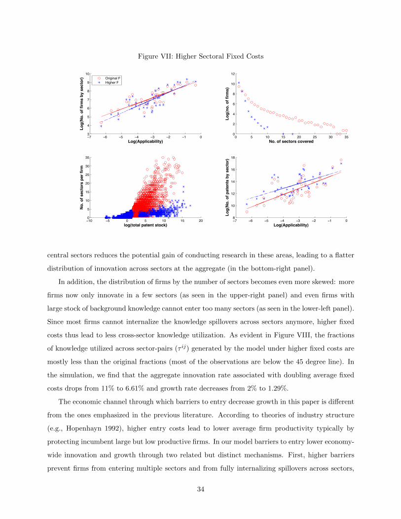
Figure VII: Higher Sectoral Fixed Costs
7 6 5 4 3 2 1 03
4
5
6
7
8
9
10
Log(Applicability)
Log(
No.
of f
irms
by s
ecto
r)
Original FHigher F
0 5 10 15 20 25 30 350
2
4
6
8
10
12
No. of sectors covered
Log(
no. o
f firm
s)10 5 0 5 10 15 20
0
5
10
15
20
25
30
35
log(total patent stock)
No.
of s
ecto
rs p
er fi
rm
7 6 5 4 3 2 1 08
10
12
14
16
18
Log(Applicability)Lo
g(N
o. o
f pat
ents
by
sect
or)
central sectors reduces the potential gain of conducting research in these areas, leading to a flatter
distribution of innovation across sectors at the aggregate (in the bottom-right panel).
In addition, the distribution of firms by the number of sectors becomes even more skewed: more
firms now only innovate in a few sectors (as seen in the upper-right panel) and even firms with
large stock of background knowledge cannot enter too many sectors (as seen in the lower-left panel).
Since most firms cannot internalize the knowledge spillovers across sectors anymore, higher fixed
costs thus lead to less cross-sector knowledge utilization. As evident in Figure VIII, the fractions
of knowledge utilized across sector-pairs (τ ij) generated by the model under higher fixed costs are
mostly less than the original fractions (most of the observations are below the 45 degree line). In
the simulation, we find that the aggregate innovation rate associated with doubling average fixed
costs drops from 11% to 6.61% and growth rate decreases from 2% to 1.29%.
The economic channel through which barriers to entry decrease growth in this paper is different
from the ones emphasized in the previous literature. According to theories of industry structure
(e.g., Hopenhayn 1992), higher entry costs lead to lower average firm productivity typically by
protecting incumbent large but low productive firms. In our model barriers to entry lower economy-
wide innovation and growth through two related but distinct mechanisms. First, higher barriers
prevent firms from entering multiple sectors and from fully internalizing spillovers across sectors,
34

Figure VIII: Fraction of Sector–j Knowledge Utilized by Sector i
0 0.2 0.4 0.6 0.8 10
0.1
0.2
0.3
0.4
0.5
0.6
0.7
0.8
0.9
1
Empirical ij
Sim
ulat
ed ij
directly blocking the knowledge circulation in the whole technology network (through lower τ ijs)
and slowing down innovation. Second, barriers to diversity reduce innovation through an indirect
research allocation effect: higher barriers distort the innovation activities away from the GPTs, the
effect of which propagates throughout the entire technology network as GPTs have the strongest
‘innovational complementarity’.45 As a consequence, the overall innovation rate decreases.
5.3.1 Experiment 2: Increasing the variance of firm idiosyncratic fixed costs, σζ
In our second experiment, we study the effect of higher variance of firm-specific fixed costs on
the aggregate innovate rate and growth rate. In Figure IX, we show that when the standard
deviation of idiosyncratic fixed cost shocks is higher, opposite to the previous experiment, the firm
distribution across sectors with different knowledge applicability becomes more even. As shown
in the left graph, relatively less firms are innovating in the central sectors than in the benchmark
case and relatively more firms exist in the peripheral sectors. This is simply because the selection
of firms into different sectors becomes more random. The fundamental knowledge linkages play
a less important role in directing the allocation of firm R&D, sector entry and exit. Related to
this observation, the middle graph shows that now less firms can cover a large number of sectors.
Firms, in general, conduct research in less sectors (as seen from the right graph). Firms become
much more homogeneous in their scope of technologies, with the standard deviation of the number
45As demonstrated in Equation (16), lower nj/ni reduces the application value of j to i. Suppose j has largeknowledge spillovers to all sectors. The disproportionate reduction in innovation in sector j would decrease theaggregate innovation rate by reducing the value of ωij in Equation (27).
35

of sectors per firm decreasing from 3.20 to 1.63.
Figure IX: Higher Standard Deviation of Firm-Specific Sectoral Fixed Costs
8 6 4 2 04
5
6
7
8
9
10
Log(Applicability)
Log(
No.
of f
irms
by s
ecto
r)
=0.5
=5
0 10 20 30 400
1
2
3
4
5
6
7
8
9
10
No. of sectors covered
Log(
no. o
f firm
s)
5 0 5 10 15 200
5
10
15
20
25
30
35
40
45
log(total patent stock)
No.
of s
ecto
rs p
er fi
rmWe can draw some intuition from inspecting the sectoral selection condition (19): a firm would
choose to conduct research in sector i if one of the following two conditions is met: (a) the firm has
accumulated enough background knowledge (i.e.∑
j ωij z
jf+θzj
nj); or (b) the firm has drawn a very
low fixed cost (ζif ). When barriers to diversity barely vary across firms (i.e. σζ → 0), firms self-select
into different sectors by ‘qualification’: firms conduct research in an area where the application value
their existing technologies is large enough to cover the fixed costs. When the variance of fixed costs
is high, firms sectoral selection is based less on qualification but more on the random idiosyncratic
fixed costs. Many firms with enough background knowledge but high fixed costs—the ‘qualified’
but ‘unlucky’ firms—cannot conduct research in a large number of areas, and firms with insufficient
background knowledge but low fixed costs—the ‘lucky’ but ‘unqualified’ firms—develop research in
more areas than in the benchmark case. As a result, the ‘lucky unqualified’ firms, naturally, would
not be able to innovate as much as the qualified firms and would devote less in R&D investment
(as according to equation (17), a firm’s optimal R&D is proportional to its existing knowledge in
related areas). On the other hand, the ‘unlucky qualified’ firms cannot utilize all their background
knowledge to develop as many new products as otherwise. Consequently, on average, firms innovate
less and cover less sectors. The fundamental factor—intersectoral knowledge linkages—plays a less
important role in directing research across sectors and firms’ selection into multiple sectors becomes
36

more random. Consistent with this intuition, we find in the simulation that the correlation between
the percentage of sector-j knowledge that is utilized in sector-i (τ ij) and the knowledge linkages
(Aij) decreases from 0.42 to 0.22. This inefficient sorting of firms into sectors with heterogenous
knowledge applicability causes a substantial fall in the economy-wide innovate rate (from 11% to
1.13%) and a large decrease in the growth rate (from 2% to 0.26%).
6 Concluding Remarks
Economic historians have long emphasized the drastic impact of ‘technological prime movers’ on
growth. Due to the lack of formal models, this insight has not been incorporated in most theories
of growth. In the present paper, we build a multi-sector model and explore the role of inter-sectoral
knowledge spillovers on firm sector entry, exit and R&D and their impact on the allocation of
research across sectors at the aggregate. We propose a measure of inter-sectoral knowledge linkages
based on a spillover network linking the knowledge receiving and sending sectors and incorporate
it into the model. We find that barriers to entry into multiple sectors lower economic growth by
blocking cross-sector knowledge circulation and prevents R&D resources from concentrating in the
GPTs.
Using patent data, we find that firms follow a general pattern when they expand across sectors:
firms start from highly applicable central sectors and gradually expand to related sectors towards
the fringe of the product network. This sequential sectoral entry has the potential to explain many
observations at firm and sector levels besides the ones shown in the current paper. Future research
could provide a better understanding of this pattern using both firm innovation and production
data, in order to understand the effects from both the production and demand sides.
The sector relatedness implied by knowledge linkages could potentially help understand the non-
random products co-production phenomenon documented by Bernard, Redding and Schott (2009a),
in which some pairs of products (e.g., fabricated metal and industrial machinery) are systematically
more likely to be produced by the same firms than other product pairs. Our analysis suggests
that the knowledge incorporated in these product pairs is highly transferable between sectors. In
addition, by emphasizing the future technological contribution from the innovating sectors to other
using sectors, our model also predicts a positive relationship between a firm’s market value and the
authority weights of its patenting sectors.46 Empirical investigation of these predictions could also
46Hall, Thoma and Torrisi (2007) find that Tobin’s q is significantly positively associated with a firm’s R&D andpatent stock, and modestly increases with the quality of patents.
37

be interesting for future research.
Our study has important implications for economic growth and R&D policies. First, govern-
ment policies directed at stimulating innovation in certain technologies need to be based on better
understanding of the inter-sectoral knowledge linkages. Heterogenous sectoral knowledge spillovers
suggest that industrial or R&D policies that favor highly applicable sectors boost growth. Second,
institutional reforms that lower sectoral entry costs reinforce the effect of industry policies, because
it can be challenging to shift to more advanced industries given the fixed cost of learning and adapt-
ing technology in new sectors. Third, competition policies that encourage joint R&D ventures in
highly related sectors can benefit growth, because firms are better able to internalize knowledge
spillovers. A successful example is China. Over the past two decades, China has significantly
shifted its industrial structure from specializing in exporting low or medium knowledge applicabile
(e.g. “Textile mill products” and “Food and kindred products”) to exporting proportionally more
highly applicable products (e.g. “Electronic components and communications equipment” and “Of-
fice computing and accounting machines”). The Chinese government has adopted a set of policies
promoting structural transformation. In fact, in a related paper (Cai and Li, 2011), we measure a
country’s product space by its export product mix, and we find that in general countries with an
export mix of higher knowledge applicability exhibit faster economic growth in subsequent years.
38

References
[1] Acemoglu D. and D. Cao. 2010. “Innovation by Entrants and Incumbents”, NBER WorkingPaper No. 16411.
[2] Akcigit U. and W. Kerr. 2010. “Growth Through Heterogeneous Innovations”, NBER workingpaper No. 16443.
[3] Aghion P. and P. Howitt. 1992. “A Model of Growth Through Creative Destruction”. Econo-metrica, Vol. 60, No.2, pp. 323-351.
[4] Atkeson, A. and A. Burstein. 2010 “Innovation, Firm Dynamics and International Trade”,Journal of Political Economy
[5] Balasubramanian, N. and J. Sivadasan. 2008. “What Happens When Firms Patent? NewEvidence from U.S. Economic Census Data”. Ross School of Business Paper No. 1090.
[6] Barseghyan, L. and R. DiCecio. 2009. “Entry Costs, Industry Structure, and Cross-CountryIncome and TFP Differences”. Federal Reserve Bank of St. Louis, working paper.
[7] Belenzon, S. and M. Schankerman. 2010. “Spreading the Word: Geography, Policy and Uni-versity Knowledge Diffusion”. CEPR Discussion Paper No. 800
[8] Bloom, N., M. Schankerman and J. V. Reenen. 2010. “Identifying Technology Spillovers andProduct Market Rivalry”. working paper.
[9] Boedo, H. and T. Mukoyama. 2010. “Evaluating the Effects of Entry Regulations and FiringCosts on International Income Differences”. University of Virginia, working paper.
[10] Bresnahan, T., and M. Trajtenberg. 1995. “General Purpose Technologies: ‘Engines ofGrowth’?,” Journal of Econometrics, Vol. 65, No. 1, pp. 83-108.
[11] Broda, C. and D. E. Weinstein. 2010. “Product Creation and Destruction: Evidence and PriceImplications”., American Economic Review, 100(3): 691-723.
[12] Buera, F., J. Kaboski and Y. Shin. 2011. “Finance and Development: A Tale of Two Sectors”,American Economic Review, 101(5), 1964-2002.
[13] Cai, J. 2010. “Knowledge Spillovers and Firm Size Heterogeneity”. University of New SouthWales, working paper.
[14] Cai, J. and N. Li. 2011. “Knowledge Linkages, Trade Composition and Income Distribution”.working paper.
[15] Carvalho, V. 2009. “Aggregate Fluctuations and the Net Work Structure of IntersectoralTrade”. University of Chicago, mimeo.
[16] Ciccone, A. 2002. “Input Chains and Industrialization”. Review of Economic Studies, Vol. 69,No. 2, pp 565-87.
[17] Conley, T. and B. Dupor. 2003. “A Spatial Analysis of Sectoral Complementarity ”. TheJournal of Political Economy, Vol. 111, No. 2, pp. 311-352.
39

[18] David, Paul. 1990. “The Dynamo and the Computer: An Historical Perspective on the ModernProductivity Paradox”. American Economic Review, Vol. 80, No. 2, pp. 355-361.
[19] Gabaix, X. 2009. “Power Laws in Economics and Finance”. Annual Review of Economics, Vol.1, pp. 255-294.
[20] Grossman, G. and E. Helpman. 1991a. “Innovation and Growth in the Global Economy”.Cambridge, MA: MIT Press.
[21] Grossman, G. and E. Helpman. 1991b. “Quality Ladders in the Theory of Growth”. Review ofEconomic Studies, 68:43-61.
[22] Hall, B, A. Jaffe, and M. Trajtenberg. 2001. “The NBER Patent Citations Data File: Lessons,Insights, and Methodological Tools”. NBER Working Paper 8498.
[23] Hausmann, R., J. Hwang and D. Rodrik. 2005. “What You Export Matters”. Journal ofEconomic Growth, 12(1):1-25.
[24] Helpman, E. (ed.). 1998. “General Purpose Technologies and Economic Growth”. Cambridgeand London: MIT Press.
[25] Hidalgo, C.A., B. Klinger, A.-L. Barabasi and R. Hausman. 2007. “The Product Space Con-ditions the Development of Nations”. Science, Vol 317, pp. 482-487.
[26] Hirschman, A. O. 1958. “The Strategy of Economic Development”. Yale University Press.
[27] Hopenhayn, H. 1992. “Entry, Exit and Firm Dynamics in Long Run Equilibrium”. Economet-rica Vol 60 No. 5, pp.1127-50.
[28] Horvath, M. 1998. “Cyclicality and Sectoral Linkages: Aggregate Fluctuations from Indepen-dent Sectoral Shocks”. Review of Economic Dynamics, Vol. 1, pp. 781-808.
[29] Hsieh C. and P. Klenow. 2009. “Misallocation and Manufacturing TFP in China and India”.Quarterly Journal of Economics, No. 124, pp. 1403-1448.
[30] Jones, C. 2010a. “Intermediate Goods and Weak Links in the Theory of Economic Develop-ment”. American Economic Journal: Macroeconomics, forthcoming.
[31] Jones, C. 2010b. “Misallocation, Economic Growth, and Input-Output Economics”. StanfordUniversity, working paper.
[32] Jones, C. 1995. “R&D–Based Models of Economic Growth”. Journal of Political Economy,103(4):759-784.
[33] Kali, R., J. Reyes, J. McGee and S. Shirrell. 2009. “Growth Networks”. University of Arkansas,mimeo.
[34] Kesten, H. 1973. “Random Difference Equations and Renewal Theory for Products of RandomMatrices”. Acta Methematica, 131: 207-248.
[35] Kleinberg, R. 1999. “Authoritative Sources in a Hyperlinked Environment” Journal of Asso-ciation for Computing Machinery, 46(5): 604-632.
[36] Klette, T. J. and S. Kortum. 2004. “Innovating Firms and Aggregate Innovation”. Journal ofPolitical Economy, Vol 112, pp. 986-1018.
40

[37] Landes, D. 1969. “The unbound Prometheus”. Cambridge University Press.
[38] Lentz, R. and D. Mortensen. 2008. “An Empirical Model of Growth Through Product Inno-vation”. Econometrica, Vol. 76, No. 6, pp. 1317-1373.
[39] Leontief, W. 1936. “Quantitative Input and Output Relations in the Economic System of theUnited States”. Review of Economics and Statistics, Vol. 18, No. 3, pp.105-125.
[40] Lucas, R.E. 1981. “Understanding Business Cycles”. In Studies in Business Cycle Theory.Cambridge, MA: MIT Press.
[41] Luttmer, E. G. 2007. “Selection, Growth, and the Size Distribution of Firms”. QuarterlyJournal of Economics, Vol. 122, No. 3, pp.1103-1144.
[42] Luttmer, E. G. 2010. “On the Mechanics of Firm Growth ”. Federal Reserve Bank Minneapolis,WP 657.
[43] Newman, M. E. J. 2003. “The Structure and Function of Complex Networks?”SIAM Review45, 167-256.
[44] Ngai, R. and R. Samiengo. 2011. “Accounting for Research and Productivity Growth AcrossIndustries”. Review of Economic Dynamics, 14(3), 475-495.
[45] Restuccia, D. and R. Rogerson. 2008. “Policy Distortions and Aggregate Productivity withHeterogeneous Establishments”. Review of Economic Dynamics, Vol.11, No. 4, pp. 707-720.
[46] Romer, P. M. 1990. “Endogenous Technological Change”. Journal of Political Economy, Vol.98, pp. 71-102.
[47] Rosenberg, N. 1982. “Inside the black box: Technology and economics”. Cambridge UniversityPress.
[48] Schmoch, U. F. Laville, P. Patel and R. Frietsch. 2003. “Linking Technology Areas to IndustrialSectors”. European Commision, DG Research.
[49] Wieser, R. 2005. “Research and Development Productivity and Spillovers: Empirical Evidenceat the Firm Level”. Journal of Economic Survey, Vol. 19, No. 4, pp. 587-621.
41

A Data Appendix
A.1 Data Sources
Firm Patenting and Patent Citations We use patent applications in the 2006 edition of the
NBER Patent Citation Data (see Hall, Jaffe and Trajtenberg, 2001 for details) to characterize firms’
innovation activities and their citations to trace the direction and intensity of knowledge flows and
to construct indices of knowledge linkages among sectors. The data provides detailed information
of every patent granted by the United States Patent and Trade Office (USPTO) and their citations
from 1976 to 2006. We summarize each firm’s patent stock in each disaggregated technological class
(intensive margin of innovation) and the number of categories (extensive margin of innovation) for
each year.47
Each patent corresponds to one of the 428 3-digit United States Patent Classification System
(USPCS) technological classes and also one of more than 800 7-digit International Patent Clas-
sification (IPC) classes. We mostly report the results based on USPCS codes, but we check for
robustness using the IPC classes. We also present some evidence based on industrial sector clas-
sification, as the model is estimated based on this categorization. To translate the data into the
industrial classifications, we use the 2005 edition of the concordance table provided by the USPTO
to map USPCS into SIC72 (Standard Industrial Classification in 1972) codes, which constructs 42
industrial sectors.48 We summarize citations made to patents that belong to the same technological
class to form the inter-sectoral knowledge spillover network.
Firm R&D and accounting data Information on firm sizes (i.e. sales or employment) and
firm’s R&D expenditure is from the U.S. Compustat database. Firm-level R&D intensity is defined
as R&D expenditure divided by sales. The industry measure of R&D intensity is the average firm
value. For robustness check, we also investigated the relationship between sectoral R&D intensity
and sectoral knowledge applicability using the median firm instead: again, they are significantly
positively related.
To obtain information of firm sizes, we use the NBER’s match of the Compustat data to the
patent data between 1970 to 2000, and keep only patenting firms.
A.2 Construction of Sectoral Knowledge Authority Weight
This network structure formed by cross-sector patent citations contains rich information about
the knowledge linkages between sectors. Some sectors contain general purpose knowledge that is
47When firms accumulate more patents over time, they not only increase the number of patents in existing patentcategories, but also expand into new categories. These two measures of firm size are highly correlated.
48The patents are classified according to either the intrinsic nature of the invention or the function for which theinvention is used or applied. It is inherently difficult to allocate the technological category to economically relevantindustries in a differentiation finer than 42 sectors, even with detailed firm level information. First, most of thepatents are issued by multi-product firms that are present in multiple SIC-4 industries. Second, in the best scenario,one only has industry information about the origin of the patents but not the industry to which the patent is actuallyapplied.
42

widely applicable in other sectors. These sectors act as knowledge authorities in the network. Other
sectors rely on knowledge from many other sectors and serve as important knowledge hubs. These
sectors resemble focused hubs that direct users to the recommended authorities in the network.
We apply an algorithm (Kleinberg, 1998) which extracts information from hyperlinked envi-
ronments to the cross-sector patent citation network. We use an index, the authority weight, to
capture the intuitive notions of the relevance, applicability and importance of knowledge in different
sectors. Sector i’s authority weight is proportional to the sum of the hub weights of the sectors that
utilize knowledge from sector i. Sector i’s hub weight is proportional to the sum of the authority
weights of the sectors that provide knowledge to sector i.
Formally, let awi denote the authority weight and hwi denote the hub weight of sector i. They
are calculated according to the following iterative algorithm:
awi = λ∑j
W ijhwj
hwi = µ∑j
W jiawj
where λ and µ are the inverse of the norms of vectors {awi}i=1,2...,428 and {hwi}i=1,2...,428, respec-
tively. W ij is the weight of the link, corresponding to the strength of citations made by sector
j (second superscript) to sector i (the first superscript). We consider two ways to measure the
weight W ij . First and most directly, we adopt the number of citations from sector j to sector i, i.e.
W ij = Citationsi←j . Second, as discussed in Hall et al (2001), industries vary in their propensity
to patent. Some sectors are especially ‘patent-sensitive’. To deal with this, we normalize citations
by the total number of patent in the citing technology class. That is, W ij measures the average
number of citations per patent in sector i that is made to sector j: W ij = Citationsi←j/PSi.
Generally speaking, a sector with a high authority weight gives large knowledge flows to sectors
with highly ranked hub weights, and a sector with a high hub weight utilizes large knowledge
flows from sectors with highly ranked authority weights. This measure of authority weight is more
suitable for our purposes than a simple citation count (i.e. Garfield’s impact factor) because not
all citations are equally important. For example, when two sectors receive the same number of
citations, it is desirable to rank the sector that receives citations from more important sectors
higher than the other sector.
A.3 Sector-pairwise Technology Distance
In addition to the sector specific authority weight, we also construct a pairwise knowledge distance
measure to facilitate our studies. Define a K dimension distance matrix D, where the {i, j}th
element, Dij = d if (Cˆd)ij > 0 and (Cˆ (d− 1))ij = 0. Cˆd denotes the dth power of the matrix
C. Dij is the shortest path distance between the nodes i and j. If (Cˆd)ij > 0, there is at least
one indirect route via other d − 1 nodes between nodes i and j. If (Cˆd)ij > 0, that means there
exists at least one d-step route between i and j. If (Cˆ (d− 1))ij = 0 is also true, then d is the
43

shortest path distance between i and j.
The mean of D’s ith column is the average distance between product i and all other products.
The average distance to other products is negatively correlated (−0.49) with our authority weight
measure, since higher authority weight products are located closer to the center of the network,
which are connected to more other products. The negative correlation is not perfect, because
the average distance ignores the volume of knowledge flow between products and the importance
of connected products. Nevertheless, the distance measure helps to understand the connectivity
between products.
Since, firms with large patent stock innovate in more sectors, their patent distribution is more
spread out in the technology space than small firms, and naturally these large firms have a higher
average distance measure of their existing product. To avoid this bias, we investigate the median
distance between the new product and firms’ existing products instead of the mean distance. Figure
A.1 shows that larger firms make significantly bigger jumps in the technology space when they enter
a new sector.
Figure A.1: Distance Between Products in the Technology Space and Firm Sizes
11.2
1.4
1.6
media
n d
ista
nce b
etw
een n
ew
secto
r and e
xis
ting s
ecto
rs
2 4 6 8 10Patent Stock (in log)
A.4 Firm’s Knowledge Applicability, Patent Stock and Multi-Technology Patent-
ing
Here, we study how innovating firms expand across technological categories given the heterogenous
authority weights of different patent classes. To investigate the innovation patterns over time, we
run the following two fixed effect regressions, controlling for firm fixed effects in each case.
ln aif,t = β0 + β1 ln psf,t + β2nif,t + µf + t+ εif,t
ln aif,t = β′0 + β′1 ln psf,t + β′2nif,t · ln psf,t + µf + t+ εif,t
44

where psf,t is firm f ’s patent stocks over all sectors, nif,t is a dummy variable equal to one if firm
f is a new entrant in sector i at time t and aif,t is the authority weight of sector i in which firm f
presents at time t. The results shown in Table A.1 are consistent with the cross-sectional findings.
The first regression results suggest that the new sectors that a firm enters are farther away from the
center of the technology space than the existing sectors. When we compare the new sectors that
different-sized firms choose to enter, larger firms tend to enter less applicable, since β′1 + β′2 < 0.
Table A.1: Firm’s Innovation Allocation, Entry and Patent Stock
Dependent Independent variables
log ps Dummy(new sector) logps log ps*Dummylog aw -0.039 -0.300 0.029 -0.111
(0.013)*** (0.010)*** (0.013)*** (-0.003)***
Note: We also control for year, firm fixed effect and clusters *** significance at 1% level. Robust standard errors are
reported in parentheses.
B Technical Appendix
B.1 An All-Sector Firm’s Optimal R&D Decision
We solve the firm’s R&D decision along the BGP. We adopt the guess-and-verify method to solve
the all-sector firm’s problem. Guess that the value of a firm is a linear combination of its accessible
knowledge capital in all the sectors in which it is producing:
V (zf,t) =K∑j=1
(vjtzjf,t
njt+ ujt
)
Substituting it back to the Bellman equation, we get
V (zf,t) =
K∑j=1
(πjtzjf,t
njt
)−
K∑i=1
K∑j=1
Rijf,t+1
1 + r
K∑j=1
(vjt+1
zjf,t +∑K
i=1
[Aji(zjtR
jif,t
)α (zif,t + θzit
)1−α]
njt+1
+ujt+1).
(30)
The first order condition with respect to Rijf,t is:
Rijf,t =njtnit
(Aijαρitv
it
M it
) 11−α
M it
(zjf,t + θzjt
njt
). (31)
45

where ρjt = 11+r
njtnjt+1
. Substituting the optimal R&D in (31) back to the Bellman equation (30), we
get:
K∑j=1
(vjtzjf,t
njt+ ujt
)=
K∑j=1
(πjzjf,t
njt
)−
K∑i=1
K∑j=1
njtnit
(Aijαρitv
it
M it
) 11−α
M it
(zjf,t + θzjt
njt
)
+1
1 + rt[
K∑j=1
vjt+1zjf,t
njt+1
+
K∑j=1
K∑i=1
vit+1
nit+1
[Aij(Aijαρitv
it
M it
) α1−α (
zjf,t + θzjt
)]+ ujt+1]
Therefore,
ujt = −K∑i=1
njtnit
(Aijαρitv
it
M it
) 11−α M i
tθzjt
njt+
1
1 + rt
K∑i=1
Aij(Aijαρitv
it
M it
) α1−α
θzjtvit+1
nit+1
+1
1 + rtujt+1
vjt
njt=
πjt
njt−
K∑i=1
K∑j=1
njtnit
(Aijαρitv
it
M it
) 11−α M i
t
njt+
1
1 + rt
K∑i=1
Aij(Aijαρitv
it
M it
) α1−α vit+1
nit+1
+1
1 + rt
vjt+1
njt+1
where M it is the total number of firms in sector i,M i
t zit = nit. The transversality condition takes
the form
limT→∞
T∏t=0
(1
1 + rt)uiT = 0,∀i
limT→∞
T∏t=0
(1
1 + rt)viTniT
= 0,∀i
In a stationary BGP equilibrium, the measure (number) of firms in a given sector is constant
M it = M i. The sectoral knowledge values and the application value of knowledge j to i are all
constant, i.e.vit = vi, uit = ui, ωijt = ωij . Now we get:
vj = (1− ρjt )−1[πj +1− αα
K∑i=1
njtnit
(Aijαρitv
i) 1
1−α M i αα−1 ]
uj = (1− 1
1 + rt)−1[
1− αα
K∑i=1
njtnit
(Aijαρitv
i) 1
1−α M i αα−1
θzjt
njt− F j ].
To simplify the notations, define the value of sector j’s knowledge in contributing to innovations
in sector i as
ωijt =1− αα
njtnit
(Aijαρitv
i) 1
1−α(M i) αα−1
46

Substituting it back, we have
vj = (1− ρjt )−1(πj +K∑i=1
ωijt ),
uj = (1 +1
r)(
K∑i=1
ωijtθzjt
njt)
and
Rijf,t =α
1− αωijt
zjf,t + θzjt
njt
To prove that ρjt , ωijt are both constants, we first need to show that the innovation rates across
sectors are the same on the BGP; therefore, we need to shownjtnjt
= ni
nj, ∀t.
The evolution of the number of varieties in sector i is:
nit+1 = nit +
∫f∈Fi,t
4zif,tdf
= nit +
K∑j=1
(Aij)1
1−α
(αρitv
i
M i
) α1−α
∫f∈Fi,t
(zjf,t + θzjt )df
= nit +
K∑j=1
[(Aij)
11−α
(αβvi
γitMi
) α1−α]
(njit + θM i
M jnjt )
where njit ≡∫
f∈Fi,t∩Fj,tzjf,tdf represents the total number of sector j goods that are produced by
firms which also produce in sector i, because not all firms in sector j is innovating and producing
in sector i. The second term in the last bracket represents the total public knowledge in sector j
that is used for innovation in sector i. Because firms can adopt public knowledge capital from every
sector when innovating, but private knowledge is limited to what sectors firms have previously
entered. The innovation rate (the growth rate of varieties) in sector i is γit = nit+1/nit. Rearranging
the terms, we have
(γit − 1)(γit)α
1−α =
(αβvi
M i
) α1−α K∑
j=1
(Aij) 1
1−α (njitnit
+ θM i
M j
njtnit
), (32)
The number of goods in every sector grows at the same speed, because inter-sector knowledge
spillovers keep all sectors on the same track. More specifically, If one sector i had been growing
more slowly than other sectors for a lengthy period, its number of goods would be extremely
small relative to other sectors. Equation (32) implies that the cross-sector knowledge spillovers
would increase γit tremendously through a large ratio njit /nit and njt/n
it until γit is the same as
the innovation rates in other sectors. Vice versa for sectors starting with a slower growth rate.
47

Therefore, in the stationary BGP equilibrium, γi = γj = γ and the distribution of sector is stable
and rank-preserving. Denotenitnjt
= ni
nj,∀t.
This result implies that ρjt = β/γ ≡ ρ and ωijt ≡ ωij are both constants, consistent with our
original guess. Therefore, we have Eq. (14), (15), (16) and (17). Now we can verify our previous
guess that the all-sector firm’s value is a linear constant-coefficient combination of its knowledge in
all sectors:
V (zf,t) =∑i∈Sf,t
vizif,tnit
+ ui.
B.2 Sectoral Innovation Rate and Research Intensity
The number of varities (patents) in sector i accumulates according to
nit+1 = nit +
∫4zif,tdf
Substitute (12) into the above equation, we get
nit+1 = nit +
∫f∈Fi,t
K∑j=1
[(Aij)
11−α
(αρitv
i
M i
) α1−α (
zjf,t + θzjt
)+ εijf,tz
if,t
]df
= nit +K∑j=1
(Aij)1
1−α
(αρitv
i
M i
) α1−α
∫f∈Fi,t
(zjf,t + θzjt
)df,
which implies the common innovation rate is
γ = 1 +
K∑j=1
nj
ni
[(Aij)
11−α
(αρvi
M i
) α1−α] ∫f∈Fi,t
(zjf,t + θzjt
)df
nit(33)
= 1 +
K∑j=1
ωijτ ij
(1− α)ρvi.
where τ ij ≡∫
f∈Fi,t
(zjf,t + θzjt
)df/nit stands for the fraction of knowledge in j that is utilized in
innovating in i. Based on (14), we can rewrite the equation above as
γ = 1 +1− ρ
(1− α)ρ
∑Ki=1
∑Kj=1 ω
ijτ ij∑Ki=1 π
i +∑K
i=1
∑Kj=1 ω
ji,
which leads to (27) after rearranging the terms.
The sectoral research intensity is defined as the overall sectoral R&D expenditure divided by
sectoral revenue: RIi ≡ 1siPY
∑Kj=1
∫f∈Fi∩Fj R
ijf df. Substitute the optimal R&D expenditure (17)
48

and (33) into the equation, we have
RIi =α
1− α1
siPY
K∑j=1
ωij
∫f∈Fi(z
jf,t + θj zjt )df
njt
=α
1− α1
siPY
K∑j=1
ωijτ ij
=αρ(γ − 1)K
PYvi
B.3 The Evolution of (Normalized) Firm Size
Based on knowledge accumulation (11), knowledge production (12) and optimal R&D investment
(17), firm f accumulates its knowledge in sector i according to
zif,t+1 = zif,t +K∑j=1
[Aij(zitR
ijf,t
)α (T jf,t
)1−α+ zjf,tε
ijf,t + θzjt ]
= zif,t +
K∑j=1
Aij
(zit
α
1− αωij
njt
)α (zjf,t + θzjt
)+ zjf,tε
ijf,t + θzjt
= zif,t +K∑j=1
Aij(Aijαρvi
M i
) α1−α (
zjf,t + θzjt
)+ zjf,tε
ijf,t + θzjt
Devide both sides by nit+1, we have
zif,t+1
nit+1
=nitnit+1
zif,tnit
+nitnit+1
K∑j
zjf,t
njt
nj
ni
[Aij(Aijαρvi
M i
) α1−α
+ εijf,t
]+
nitnit+1
K∑j=1
θzjtnit
[Aij(Aijαρvi
M i
) α1−α]
=1
γ
zif,tnit
+
K∑j
zjf,t
njt
nj
ni(Aij
(Aijαρvi
M i
) α1−α
+ εijf,t)
+1
γ
K∑j=1
θj
M j
nj
ni
[Aij(Aijαρvi
M i
) α1−α]
=1
γ
zif,tnit
+K∑j
zjf,t
njt
(ωij
(1− α)ρvi+nj
niεij1f,t
)+1
γ
K∑j=1
θj
M j
ωij
(1− α)ρvi
Define φijf,t ≡1γ
(1{if i=j} + ξij + nj
niεijf,t
), ψijf ≡
ξij
γ , we can rewrite the above equation as in (25).
B.4 Steady State General Equilibrium Conditions
The equilibrium innovation rate (27) can be rewritten as γ = 1+ 1(1−α)ρvi
[∫f∈Fi
∑Kj=1
ωijzjfnj
df +∑K
j=1θωijM i
Mj
].
Keston (1973) can be applied to show that the normalized firm size in each sector zif/ni follows
a Pareto distribution, firm’s private knowledge value in sector i, kif ≡∑K
j=1
ωijzjfnj
is also Pareto-
distributed because linear combination of Pareto distributions is still Pareto.Suppose ai is hte
49

Pareto parameter of the distribution of kif , the sectoral entry condition provides a lower bound
of the distribution, ki∗ = F − r1+ru
i. Then∫f∈Fi
∑Kj=1
ωijzjfnj
df = M i aiki∗
ai−1= M i ai
ai−1(F − r
1+rui).
Therefore, we can express the total innovation rate in aggregate variables as follows
γ = 1 +1
(1− α)ρvi
M i ai
ai − 1(F − r
1 + rui)+
K∑j=1
θωijM i
M j
Similarly, assume F (·) is the cdf of normalized firm size distribution with the shape parameter
given by bi and the lower bound of this distribution given by∑K
j=1ωij
(1−α)ρviγθM i (see (25)) then we
have
1 =
∫f∈Fi
zifnidF i(
zi
ni)M i =
bi
bi − 1
K∑j=1
ωijθ
(1− α)ρviγ.
Unfortunately, we cannot derive a close form expression for ai and bi, although they both depend
on other parameters in the economy, such as θ, σε, σζ etc. We thus simulate the model to generate
the shape parameters for the distribution of firm’s private knowledge value and the distribution of
firm size in different sectors.
Therefore, the general equilibrium conditions are characterized by the following K2 + 4K + 4
equations with an equal number of endogenous variables: {vi, ui,M i}i, {nj
ni, ωij}ij , ρ, γ, r, PY.
vj =1
1− ρ(PY
σK+∑i
ωij)
ωij =nj
ni1− αα
(Aijαρvi)1
1−α (M i)αα−1
ui =r
1 + r
K∑j
θωij
M j
1 = β(1 + r)γη−11−σ
ρ = βγη+σ−21−σ
PY = L+ r∑i
[vi −M i
(1 + r
rF − ui
)]
L =σ − 1
σPY +
K∑i=1
[αρ(γ − 1)vi +M iF
]γ = 1 +
1
(1− α)ρvi
M i ai
ai − 1(F − r
1 + rui)+
K∑j=1
θωijM i
M j
1 =
bi
bi − 1
K∑j=1
ωijθ
(1− α)ρviγ
50

Table A.1: List of 42 Sectors Ranked According to the Authority Weight
Field Sector Name Authority Weight Hub Weight
36 Railroad equipment 0.00017 0.0002138 Miscellaneous transportation equipment 0.00022 0.0002737 Motorcycles, bicycles, and parts 0.00024 0.0002235 Ship and boat building and repairing 0.00033 0.0002928 Household appliances 0.00041 0.0007025 Miscellaneous machinery, except electrical 0.00045 0.0003314 Primary ferrous products 0.00059 0.0009034 Guided missiles and space vehicles and parts 0.00069 0.000401 Food and kindred products 0.00093 0.0007840 Aircraft and parts 0.00125 0.0010839 Ordinance except missiles 0.00133 0.001027 Soaps, detergents, cleaners, perfumes, cosmetics and toiletries 0.00189 0.0015811 Petroleum and natural gas extraction 0.00190 0.001703 Industrial inorganic chemistry 0.00232 0.0029117 Engines and turbines 0.00268 0.003038 Paints, varnishes, lacquers, enamels, and allied products 0.00273 0.0034624 Refrigeration and service industry machinery 0.00284 0.0030415 Primary and secondary non-ferrous metals 0.00329 0.003589 Miscellaneous chemical products 0.00429 0.004285 Plastics materials and synthetic resins 0.00466 0.0065718 Farm and garden machinery and equipment 0.00528 0.0059319 Construction, mining and material handling machinery and equipment 0.00575 0.0061413 Stone, clay, glass and concrete products 0.00670 0.0074033 Motor vehicles and other motor vehicle equipment 0.00712 0.006932 Textile mill products 0.00776 0.008294 Industrial organic chemistry 0.00834 0.008986 Agricultural chemicals 0.00865 0.0065120 Metal working machinery and equipment 0.00942 0.0114310 Drugs and medicines 0.00982 0.0073729 Electrical lighting and wiring equipment 0.01623 0.0127830 Miscellaneous electrical machinery, equipment and supplies 0.01861 0.0204822 Special industry machinery, except metal working 0.02046 0.0203427 Electrical industrial apparatus 0.02110 0.0226723 General industrial machinery and equipment 0.02431 0.0259216 Fabricated metal products 0.02988 0.0352931 Radio and television receiving equipment except communication types 0.03663 0.0481542 All Other Sectors 0.03800 0.0393612 Rubber and miscellaneous plastics products 0.04078 0.0432926 Electrical transmission and distribution equipment 0.04212 0.0512021 Office computing and accounting machines 0.32458 0.2949541 Professional and scientific instruments 0.56854 0.5655132 Electronic components and accessories and communications equipment 0.74939 0.76206
51
Top Related