


Languages
Pages
Legal

Gradient Boosted Regression Trees
scikit
Peter Prettenhofer (@pprett)DataRobot
Gilles Louppe (@glouppe)Universite de Liege, Belgium

Motivation

Motivation

Outline
1 Basics
2 Gradient Boosting
3 Gradient Boosting in scikit-learn
4 Case Study: California housing

About us
Peter
• @pprett
• Python & ML ∼ 6 years
• sklearn dev since 2010
Gilles
• @glouppe
• PhD student (Liege,Belgium)
• sklearn dev since 2011Chief tree hugger

Outline
1 Basics
2 Gradient Boosting
3 Gradient Boosting in scikit-learn
4 Case Study: California housing
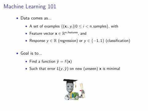
Machine Learning 101
• Data comes as...
• A set of examples {(xi , yi )|0 ≤ i < n samples}, with
• Feature vector x ∈ Rn features, and
• Response y ∈ R (regression) or y ∈ {−1, 1} (classification)
• Goal is to...
• Find a function y = f (x)
• Such that error L(y , y) on new (unseen) x is minimal

Classification and Regression Trees [Breiman et al, 1984]
MedInc <= 5.04
MedInc <= 3.07 MedInc <= 6.82
AveRooms <= 4.31 AveOccup <= 2.37
1.62 1.16 2.79 1.88
AveOccup <= 2.74 MedInc <= 7.82
3.39 2.56 3.73 4.57
sklearn.tree.DecisionTreeClassifier|Regressor
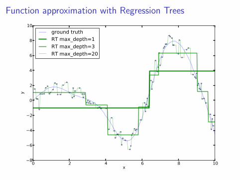
Function approximation with Regression Trees
0 2 4 6 8 10x
8
6
4
2
0
2
4
6
8
10y
ground truthRT max_depth=1RT max_depth=3RT max_depth=20
Deprecated
• Nowadays seldom used alone
• Ensembles: Random Forest, Bagging, or Boosting(see sklearn.ensemble)

Function approximation with Regression Trees
0 2 4 6 8 10x
8
6
4
2
0
2
4
6
8
10y
ground truthRT max_depth=1RT max_depth=3RT max_depth=20
Deprecated
• Nowadays seldom used alone
• Ensembles: Random Forest, Bagging, or Boosting(see sklearn.ensemble)
Outline
1 Basics
2 Gradient Boosting
3 Gradient Boosting in scikit-learn
4 Case Study: California housing

Gradient Boosted Regression Trees
Advantages
• Heterogeneous data (features measured on different scale)
• Supports different loss functions (e.g. huber)
• Automatically detects (non-linear) feature interactions
Disadvantages
• Requires careful tuning
• Slow to train (but fast to predict)
• Cannot extrapolate

Boosting
AdaBoost [Y. Freund & R. Schapire, 1995]
• Ensemble: each member is an expert on the errors of itspredecessor
• Iteratively re-weights training examples based on errors
2 1 0 1 2 3x0
2
1
0
1
2
x1
2 1 0 1 2 3x0
2 1 0 1 2 3x0
2 1 0 1 2 3x0
sklearn.ensemble.AdaBoostClassifier|Regressor
Huge success
• Viola-Jones Face Detector (2001)
• Freund & Schapire won the Godel prize 2003

Gradient Boosting [J. Friedman, 1999]
Statistical view on boosting
• ⇒ Generalization of boosting to arbitrary loss functions
Residual fitting
2 6 10x
2.0
1.5
1.0
0.5
0.0
0.5
1.0
1.5
2.0
2.5
y
Ground truth
2 6 10x
∼
tree 1
2 6 10x
+
tree 2
2 6 10x
+
tree 3
sklearn.ensemble.GradientBoostingClassifier|Regressor

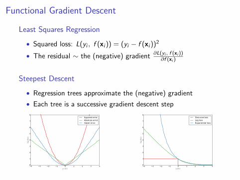
Functional Gradient Descent
Least Squares Regression
• Squared loss: L(yi , f (xi )) = (yi − f (xi ))2
• The residual ∼ the (negative) gradient ∂L(yi , f (xi ))∂f (xi )
Steepest Descent
• Regression trees approximate the (negative) gradient
• Each tree is a successive gradient descent step
4 3 2 1 0 1 2 3 4y−f(x)
0
1
2
3
4
5
6
7
8
L(y,f
(x))
Squared errorAbsolute errorHuber error
4 3 2 1 0 1 2 3 4y ·f(x)
0
1
2
3
4
5
6
7
8
L(y,f
(x))
Zero-one lossLog lossExponential loss
Outline
1 Basics
2 Gradient Boosting
3 Gradient Boosting in scikit-learn
4 Case Study: California housing

GBRT in scikit-learn
How to use it
>>> from sklearn.ensemble import GradientBoostingClassifier
>>> from sklearn.datasets import make_hastie_10_2
>>> X, y = make_hastie_10_2(n_samples=10000)
>>> est = GradientBoostingClassifier(n_estimators=200, max_depth=3)
>>> est.fit(X, y)
...
>>> # get predictions
>>> pred = est.predict(X)
>>> est.predict_proba(X)[0] # class probabilities
array([ 0.67, 0.33])
Implementation
• Written in pure Python/Numpy (easy to extend).
• Builds on top of sklearn.tree.DecisionTreeRegressor (Cython).
• Custom node splitter that uses pre-sorting (better for shallow trees).
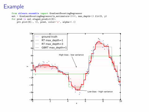
Examplefrom sklearn.ensemble import GradientBoostingRegressor
est = GradientBoostingRegressor(n_estimators=2000, max_depth=1).fit(X, y)
for pred in est.staged_predict(X):
plt.plot(X[:, 0], pred, color=’r’, alpha=0.1)
0 2 4 6 8 10x
8
6
4
2
0
2
4
6
8
10
y
High bias - low variance
Low bias - high variance
ground truthRT max_depth=1RT max_depth=3GBRT max_depth=1

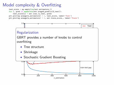
Model complexity & Overfittingtest_score = np.empty(len(est.estimators_))
for i, pred in enumerate(est.staged_predict(X_test)):
test_score[i] = est.loss_(y_test, pred)
plt.plot(np.arange(n_estimators) + 1, test_score, label=’Test’)
plt.plot(np.arange(n_estimators) + 1, est.train_score_, label=’Train’)
0 200 400 600 800 1000n_estimators
0.0
0.5
1.0
1.5
2.0
Err
or
Lowest test error
train-test gap
TestTrain
Regularization
GBRT provides a number of knobs to controloverfitting
• Tree structure
• Shrinkage
• Stochastic Gradient Boosting

Regularization: Tree structure
• The max depth of the trees controls the degree of features interactions
• Use min samples leaf to have a sufficient nr. of samples per leaf.
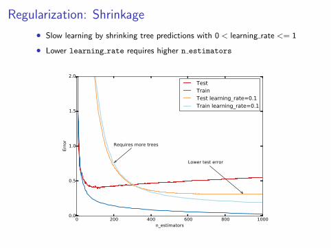
Regularization: Shrinkage
• Slow learning by shrinking tree predictions with 0 < learning rate <= 1
• Lower learning rate requires higher n estimators
0 200 400 600 800 1000n_estimators
0.0
0.5
1.0
1.5
2.0
Err
or
Requires more trees
Lower test error
Test Train Test learning_rate=0.1
Train learning_rate=0.1
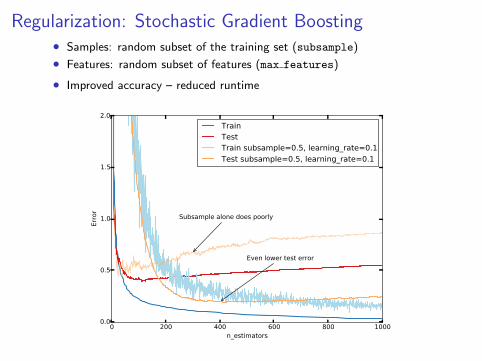
Regularization: Stochastic Gradient Boosting• Samples: random subset of the training set (subsample)
• Features: random subset of features (max features)
• Improved accuracy – reduced runtime
0 200 400 600 800 1000n_estimators
0.0
0.5
1.0
1.5
2.0
Err
or
Even lower test error
Subsample alone does poorly
Train Test Train subsample=0.5, learning_rate=0.1
Test subsample=0.5, learning_rate=0.1
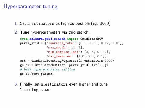
Hyperparameter tuning
1. Set n estimators as high as possible (eg. 3000)
2. Tune hyperparameters via grid search.
from sklearn.grid_search import GridSearchCV
param_grid = {’learning_rate’: [0.1, 0.05, 0.02, 0.01],
’max_depth’: [4, 6],
’min_samples_leaf’: [3, 5, 9, 17],
’max_features’: [1.0, 0.3, 0.1]}
est = GradientBoostingRegressor(n_estimators=3000)
gs_cv = GridSearchCV(est, param_grid).fit(X, y)
# best hyperparameter setting
gs_cv.best_params_
3. Finally, set n estimators even higher and tunelearning rate.
Outline
1 Basics
2 Gradient Boosting
3 Gradient Boosting in scikit-learn
4 Case Study: California housing

Case Study
California Housing dataset
• Predict log(medianHouseValue)
• Block groups in 1990 census
• 20.640 groups with 8 features(median income, median age, lat,lon, ...)
• Evaluation: Mean absolute erroron 80/20 split
Challenges
• Heterogeneous features
• Non-linear interactions
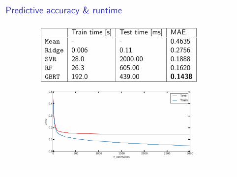
Predictive accuracy & runtime
Train time [s] Test time [ms] MAE
Mean - - 0.4635Ridge 0.006 0.11 0.2756SVR 28.0 2000.00 0.1888RF 26.3 605.00 0.1620GBRT 192.0 439.00 0.1438
0 500 1000 1500 2000 2500 3000n_estimators
0.0
0.1
0.2
0.3
0.4
0.5
err
or
TestTrain

Model interpretation
Which features are important?
>>> est.feature_importances_
array([ 0.01, 0.38, ...])
0.00 0.02 0.04 0.06 0.08 0.10 0.12 0.14 0.16 0.18Relative importance
HouseAge
Population
AveBedrms
Latitude
AveOccup
Longitude
AveRooms
MedInc

Model interpretationWhat is the effect of a feature on the response?
from sklearn.ensemble import partial_dependence import as pd
features = [’MedInc’, ’AveOccup’, ’HouseAge’, ’AveRooms’,
(’AveOccup’, ’HouseAge’)]
fig, axs = pd.plot_partial_dependence(est, X_train, features,
feature_names=names)
1.5 3.0 4.5 6.0 7.5MedInc
0.4
0.2
0.0
0.2
0.4
0.6
Part
ial dependence
2.0 2.5 3.0 3.5 4.0 4.5AveOccup
0.4
0.2
0.0
0.2
0.4
0.6
Part
ial dependence
10 20 30 40 50 60HouseAge
0.4
0.2
0.0
0.2
0.4
0.6
Part
ial dependence
4 5 6 7 8AveRooms
0.4
0.2
0.0
0.2
0.4
0.6
Part
ial dependence
2.0 2.5 3.0 3.5 4.0AveOccup
10
20
30
40
50
House
Age
-0.1
2
-0.0
5
0.0
2
0.09
0.1
6
0.23
Partial dependence of house value on nonlocation featuresfor the California housing dataset
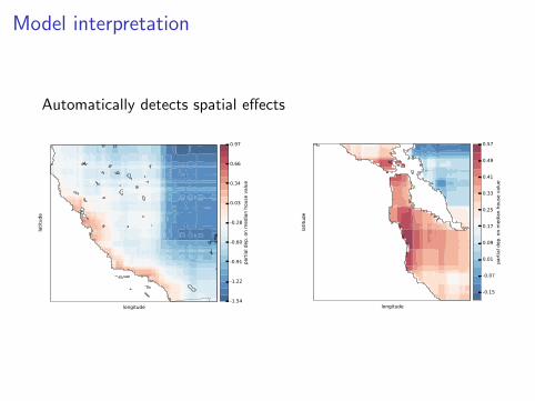
Model interpretation
Automatically detects spatial effects
longitude
lati
tude
-1.54
-1.22
-0.91
-0.60
-0.28
0.03
0.34
0.66
0.97
part
ial dep.
on m
edia
n h
ouse
valu
e
longitudela
titu
de
-0.15
-0.07
0.01
0.09
0.17
0.25
0.33
0.41
0.49
0.57
part
ial dep.
on m
edia
n h
ouse
valu
e

Summary
• Flexible non-parametric classification and regression technique
• Applicable to a variety of problems
• Solid, battle-worn implementation in scikit-learn

Thanks! Questions?

Benchmarks
0.00.20.40.60.81.01.2
Err
or
gbmsklearn-0.15
0.00.51.01.52.02.53.0
Tra
in t
ime
Arc
ene
Bost
on
Calif
orn
ia
Covty
pe
Exam
ple
10
.2
Expedia
Madelo
n
Sola
r
Spam
YahooLT
RC
bio
resp
dataset
0.0
0.2
0.4
0.6
0.8
1.0
Test
tim
e

Tipps & Tricks 1
Input layout
Use dtype=np.float32 to avoid memory copies and fortan layout for slight
runtime benefit.
X = np.asfortranarray(X, dtype=np.float32)
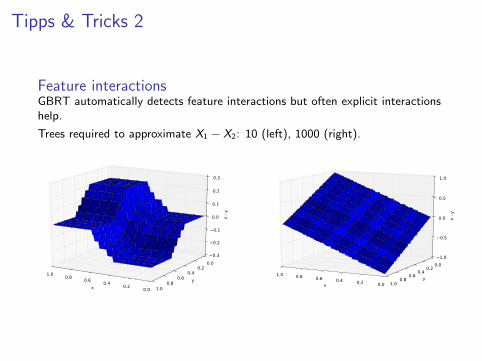
Tipps & Tricks 2
Feature interactionsGBRT automatically detects feature interactions but often explicit interactionshelp.
Trees required to approximate X1 − X2: 10 (left), 1000 (right).
x 0.00.2
0.40.6
0.81.0
y
0.00.2
0.40.6
0.81.0
x -
y
0.3
0.2
0.1
0.0
0.1
0.2
0.3
x 0.00.20.40.60.81.0y
0.00.2
0.40.6
0.81.0
x -
y
1.0
0.5
0.0
0.5
1.0
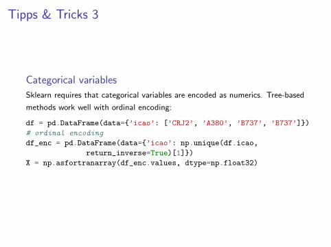
Tipps & Tricks 3
Categorical variables
Sklearn requires that categorical variables are encoded as numerics. Tree-based
methods work well with ordinal encoding:
df = pd.DataFrame(data={’icao’: [’CRJ2’, ’A380’, ’B737’, ’B737’]})
# ordinal encoding
df_enc = pd.DataFrame(data={’icao’: np.unique(df.icao,
return_inverse=True)[1]})
X = np.asfortranarray(df_enc.values, dtype=np.float32)
Top Related