


Languages
Pages
Legal


Gradient Boosted Decision Trees on Hadoop
jerry ye | jyh-herng chow | jiang chen | zhaohui zheng

Agenda
Overview
› GBDT
› Implementations
› Related Work
GBDT
› Learning a tree
› Boosting
Method
› MapReduce Implementations
› MPI Implementation
Results
Conclusion
Introduction
Gradient Boosted Decision Trees (GBDT) is a machine learning algorithm that iteratively constructs an ensemble of weak decision tree learners through boosting.
What is GBDT?
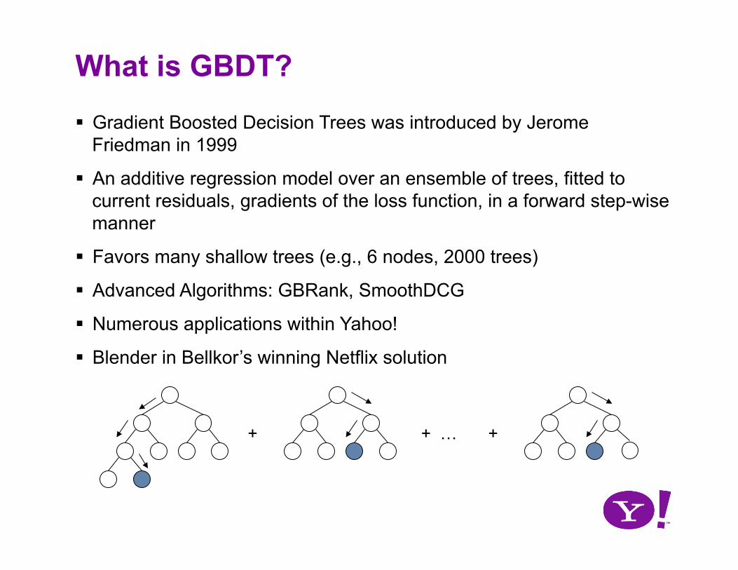
Gradient Boosted Decision Trees was introduced by Jerome Friedman in 1999
An additive regression model over an ensemble of trees, fitted to current residuals, gradients of the loss function, in a forward step-wise manner
Favors many shallow trees (e.g., 6 nodes, 2000 trees)
Advanced Algorithms: GBRank, SmoothDCG
Numerous applications within Yahoo!
Blender in Bellkor’s winning Netflix solution
+ + + …
Advantages
Feature normalization is not required
Feature selection is inherently performed during the learning process
Not prone to collinear/identical features
Models are relatively easy to interpret
Easy to specify different loss functions
Disadvantages
Boosting is a sequential process, not parallelizable
Compute intensive
Can perform poorly on high dimensional sparse data, e.g. bag of words
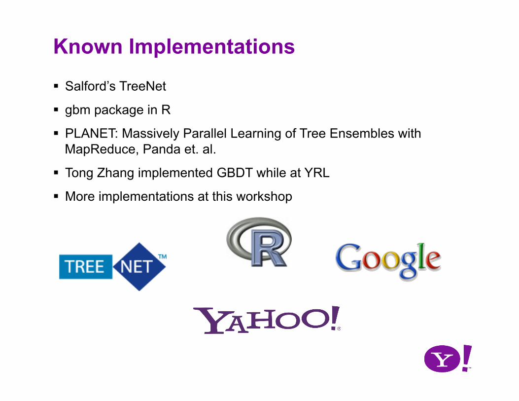
Known Implementations
Salford’s TreeNet
gbm package in R
PLANET: Massively Parallel Learning of Tree Ensembles with MapReduce, Panda et. al.
Tong Zhang implemented GBDT while at YRL
More implementations at this workshop

Algorithm Overview
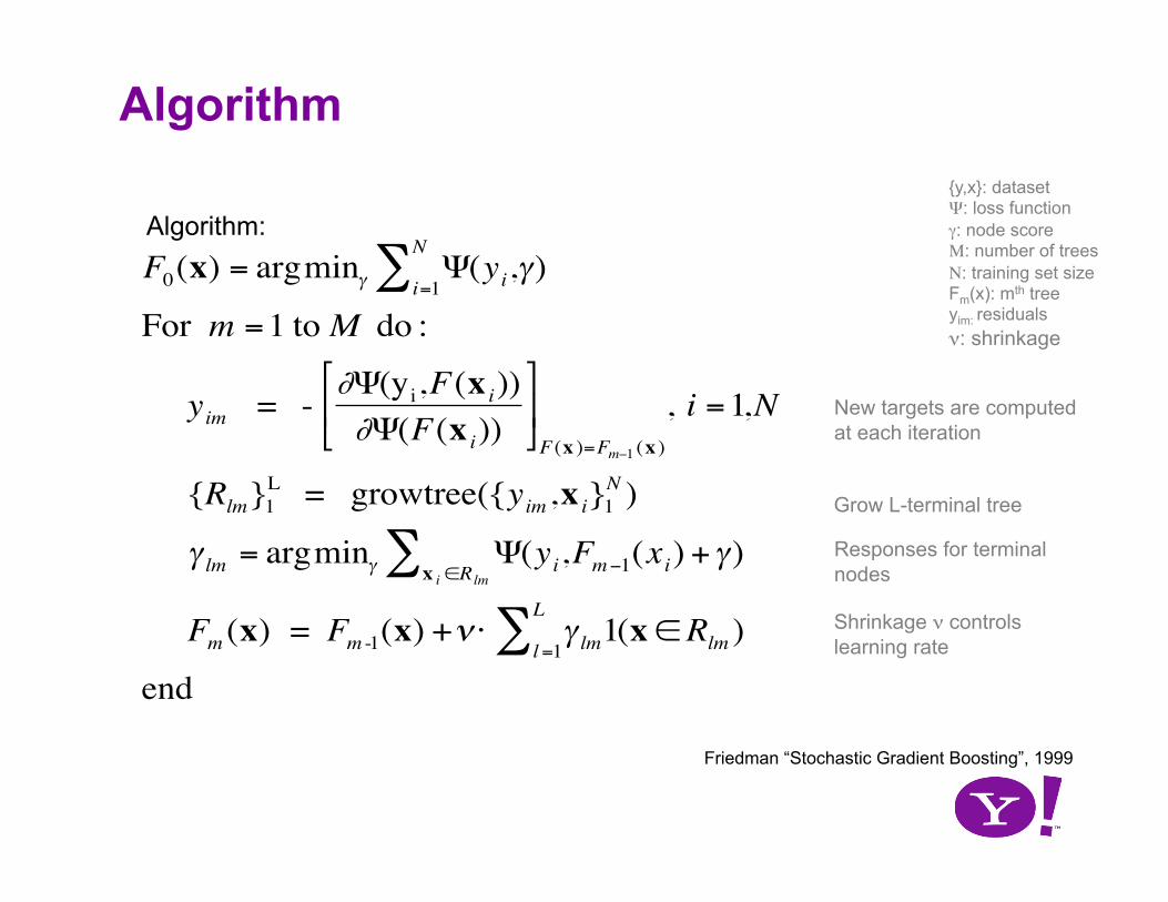
Algorithm
Algorithm:
€
F0(x) = argminγ Ψ(yi,γ)i=1
N∑
For m =1 to M do :
yim = - ∂Ψ(yi,F(x i))∂Ψ(F(x i))
⎡
⎣ ⎢
⎤
⎦ ⎥ F (x )=Fm−1 (x )
, i =1,N
{Rlm}1L = growtree({yim,x i}1
N )
γ lm = argminγ Ψ(yi,Fm−1(xi) +γ)x i ∈Rlm
∑
Fm (x) = Fm -1(x) +ν⋅ γ lm1(x∈Rlm )l=1
L∑
end
Friedman “Stochastic Gradient Boosting”, 1999
New targets are computed at each iteration
Responses for terminal nodes
Shrinkage ν controls learning rate
Grow L-terminal tree
{y,x}: dataset Ψ: loss function γ: node score Μ: number of trees Ν: training set size Fm(x): mth tree yim: residuals ν: shrinkage
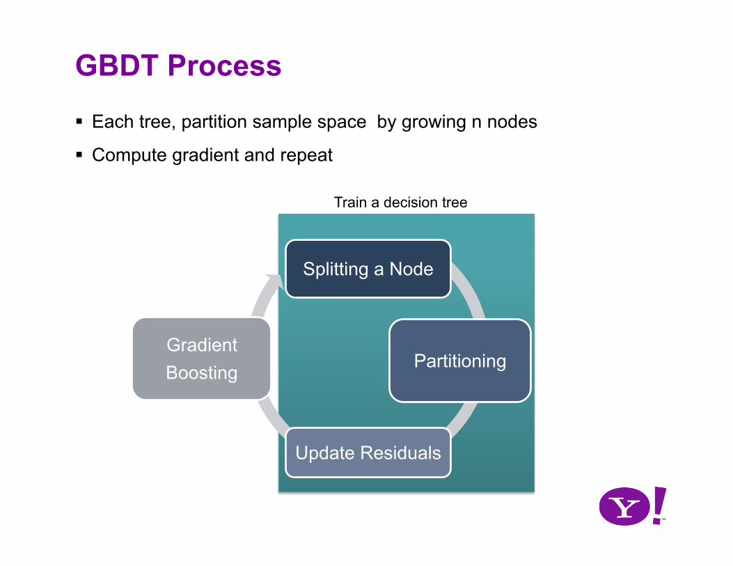
GBDT Process
Each tree, partition sample space by growing n nodes
Compute gradient and repeat
Splitting a Node
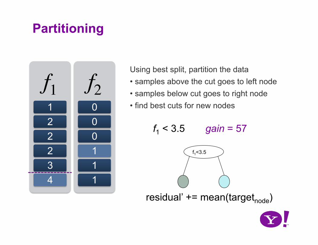
Partitioning
Update Residuals
Gradient Boosting
Train a decision tree
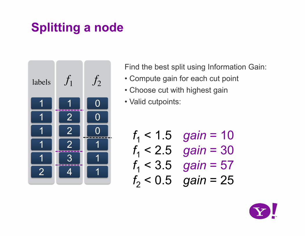
labels
1 1 1 1 1 2
f1
1 2 2 2 3 4
f2
0 0 0 1 1 1
Find the best split using Information Gain: • Compute gain for each cut point • Choose cut with highest gain • Valid cutpoints:
f1 < 1.5 f1 < 2.5 f1 < 3.5 f2 < 0.5
gain = 10 gain = 30 gain = 57 gain = 25
Splitting a node
f1 1 2 2 2 3 4
f2 0 0 0 1 1 1
Using best split, partition the data • samples above the cut goes to left node • samples below cut goes to right node • find best cuts for new nodes
f1 < 3.5 gain = 57
f1<3.5
residual’ += mean(targetnode)
Partitioning
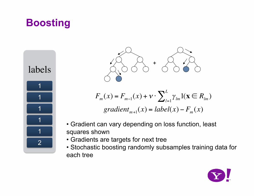
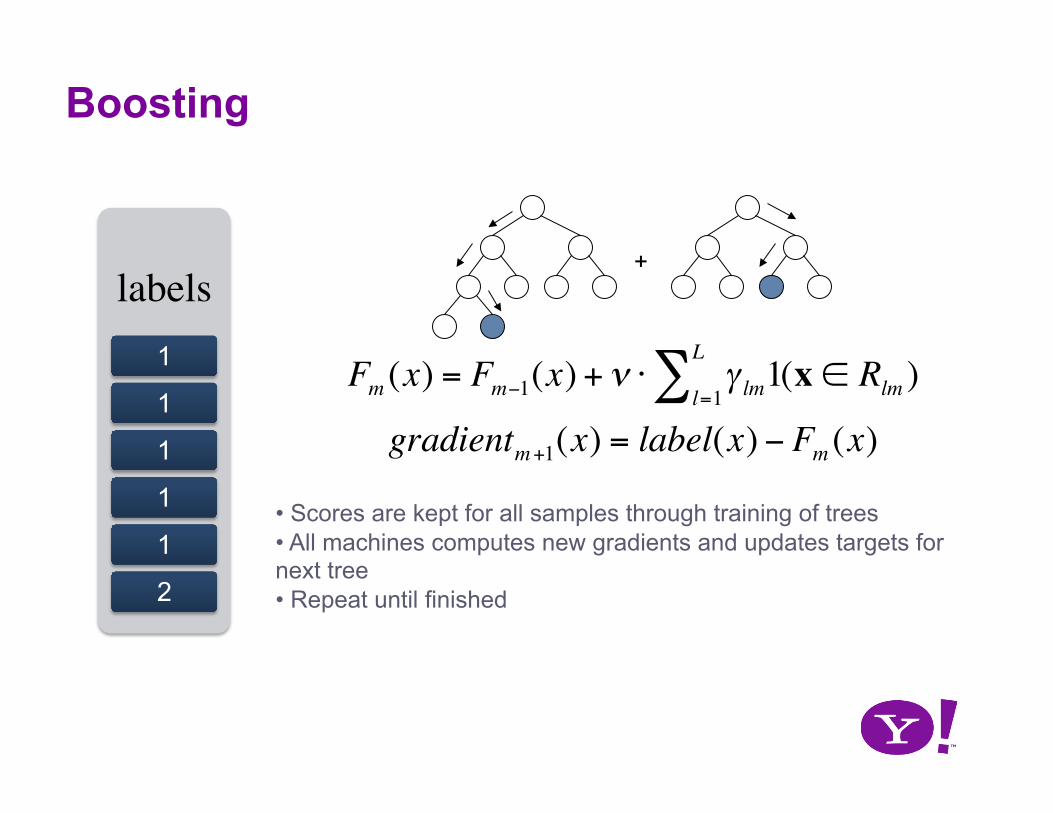
Boosting
€
Fm (x) = Fm−1(x) + ν ⋅ γ lm1(x ∈ Rlm )l=1
L∑
gradientm+1(x) = label(x) − Fm (x)
labels 1
1
1
1
1
2
• Gradient can vary depending on loss function, least squares shown • Gradients are targets for next tree • Stochastic boosting randomly subsamples training data for each tree
+
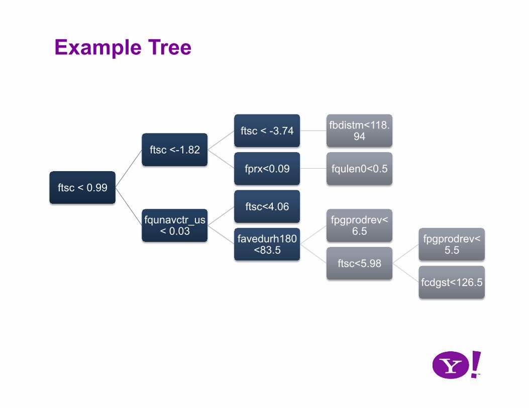
Example Tree
ftsc < 0.99
ftsc <-1.82
ftsc < -3.74 fbdistm<118.94
fprx<0.09 fqulen0<0.5
fqunavctr_us < 0.03
ftsc<4.06
favedurh180<83.5
fpgprodrev<6.5
ftsc<5.98
fpgprodrev<5.5
fcdgst<126.5

MapReduce Implementations
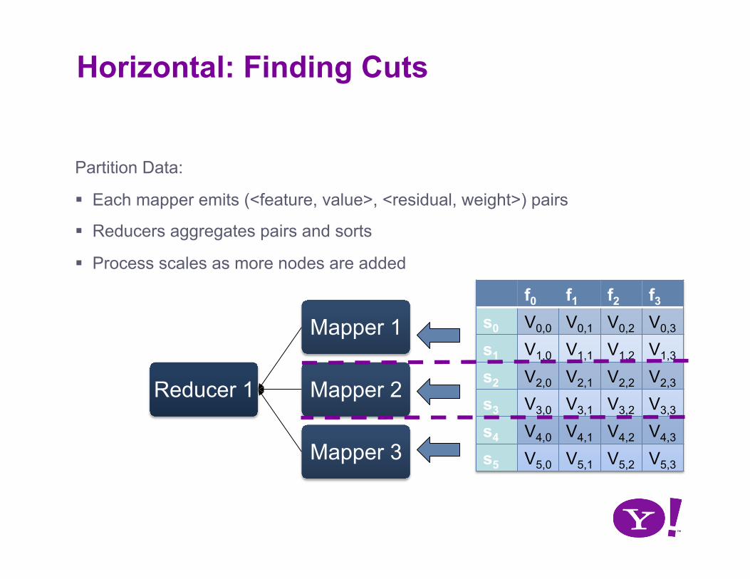
f0 f1 f2 f3
s0 V0,0 V0,1 V0,2 V0,3
s1 V1,0 V1,1 V1,2 V1,3
s2 V2,0 V2,1 V2,2 V2,3
s3 V3,0 V3,1 V3,2 V3,3
s4 V4,0 V4,1 V4,2 V4,3
s5 V5,0 V5,1 V5,2 V5,3
Horizontal: Finding Cuts
Partition Data:
Each mapper emits (<feature, value>, <residual, weight>) pairs
Reducers aggregates pairs and sorts
Process scales as more nodes are added
Reducer 1
Mapper 1
Mapper 2
Mapper 3
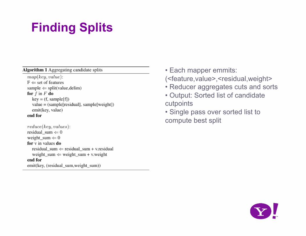
Finding Splits
• Each mapper emmits: (<feature,value>,<residual,weight> • Reducer aggregates cuts and sorts • Output: Sorted list of candidate cutpoints • Single pass over sorted list to compute best split
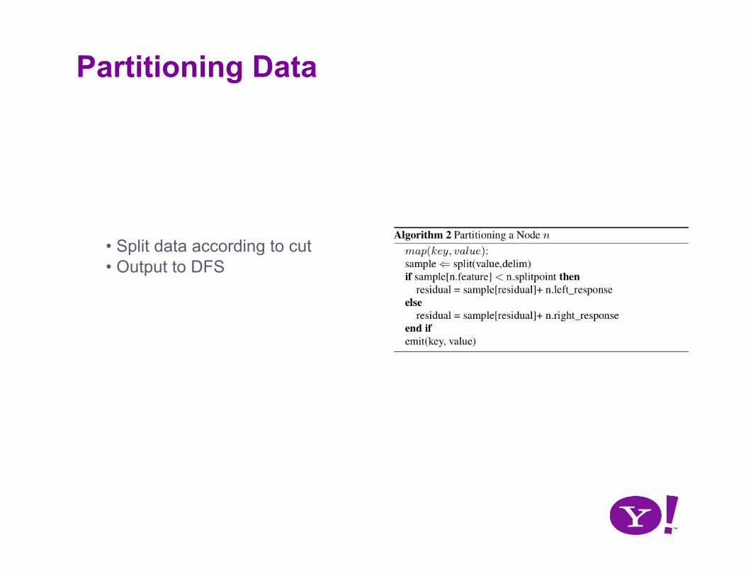
Partitioning Data
• Split data according to cut • Output to DFS
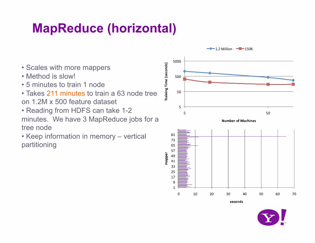
MapReduce (horizontal)
• Scales with more mappers • Method is slow! • 5 minutes to train 1 node • Takes 211 minutes to train a 63 node tree on 1.2M x 500 feature dataset • Reading from HDFS can take 1-2 minutes. We have 3 MapReduce jobs for a tree node • Keep information in memory – vertical partitioning
f0 f1 f2 f3
s0 V0,0 V0,1 V0,2 V0,3
s1 V1,0 V1,1 V1,2 V1,3
s2 V2,0 V2,1 V2,2 V2,3
s3 V3,0 V3,1 V3,2 V3,3
s4 V4,0 V4,1 V4,2 V4,3
s5 V5,0 V5,1 V5,2 V5,3
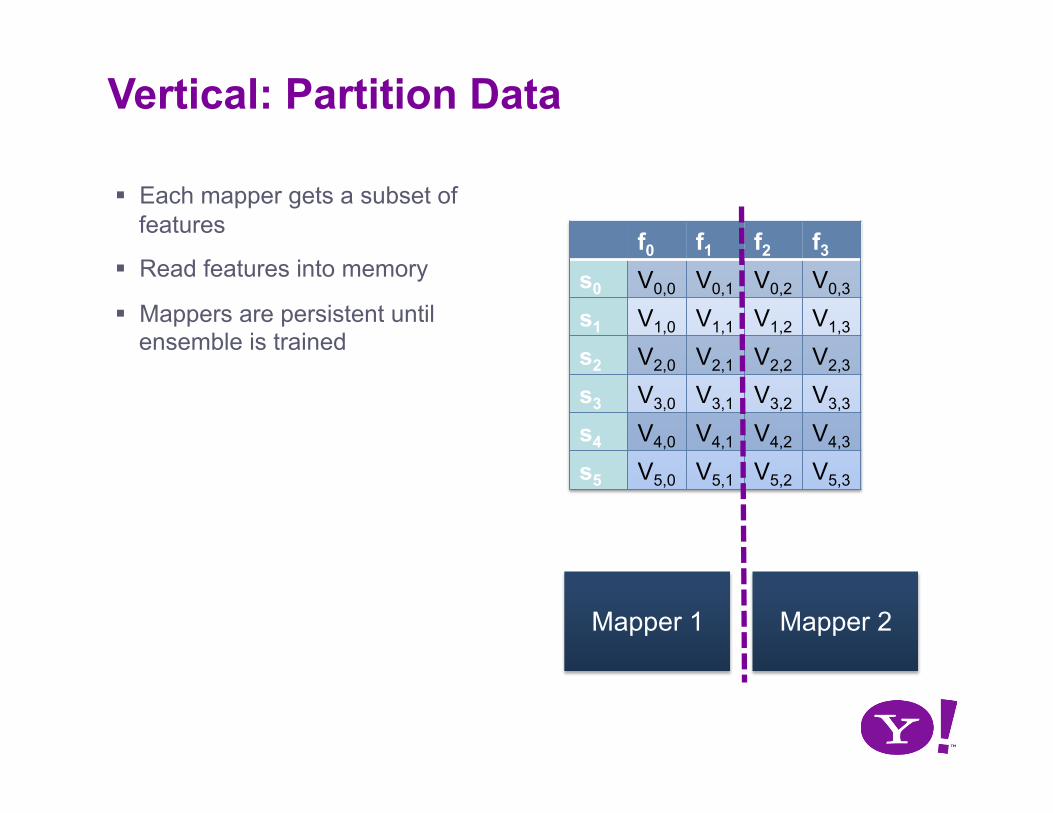
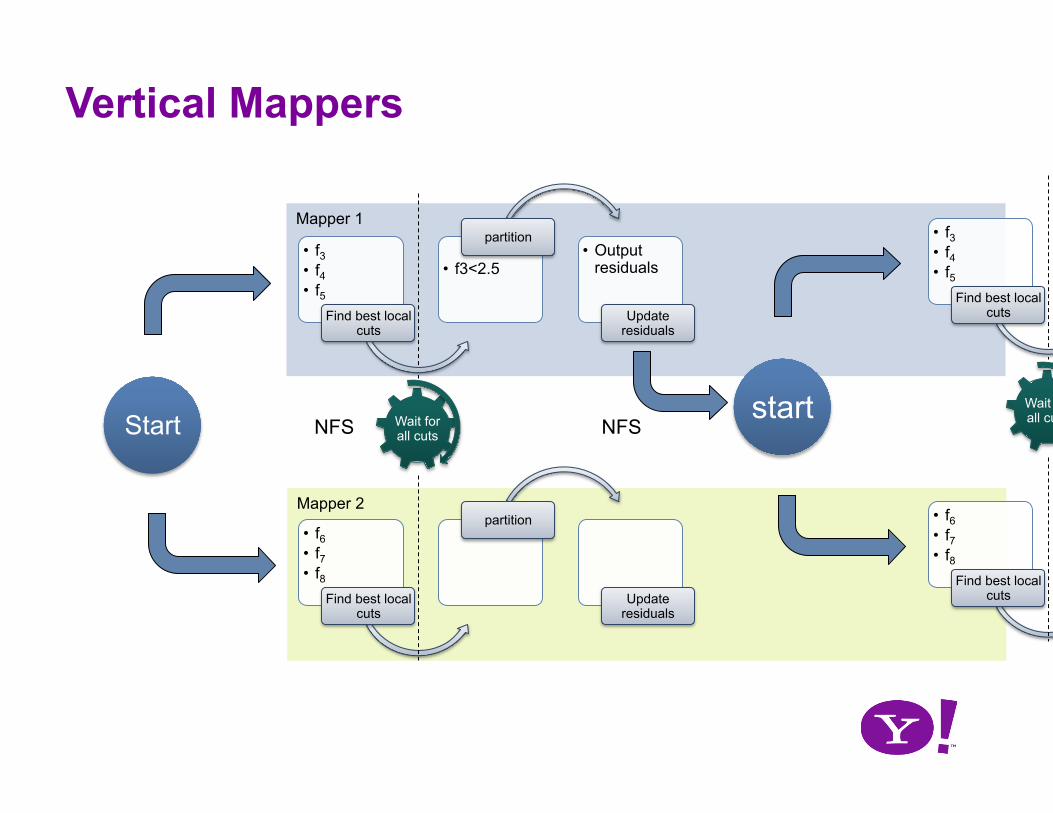
Vertical: Partition Data
Each mapper gets a subset of features
Read features into memory
Mappers are persistent until ensemble is trained
Mapper 1 Mapper 2
Mapper 2
Mapper 1
• f6 • f7 • f8
Find best local cuts
partition
Update residuals
Wait for all cuts Start
• f3 • f4 • f5
Find best local cuts
• f3<2.5
partition • Output
residuals
Update residuals
• f6 • f7 • f8
Find best local cuts
Wait for all cuts start
• f3 • f4 • f5
Find best local cuts
NFS NFS
Vertical Mappers

MPI Implementation
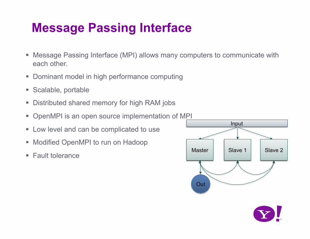
Message Passing Interface
Message Passing Interface (MPI) allows many computers to communicate with each other.
Dominant model in high performance computing
Scalable, portable
Distributed shared memory for high RAM jobs
OpenMPI is an open source implementation of MPI
Low level and can be complicated to use
Modified OpenMPI to run on Hadoop
Fault tolerance Master Slave 1 Slave 2
Out
Input
labels
1
1
1
1
1
2
f1
1
2
2
2
3
4
f2 0
0
0
1
1
1
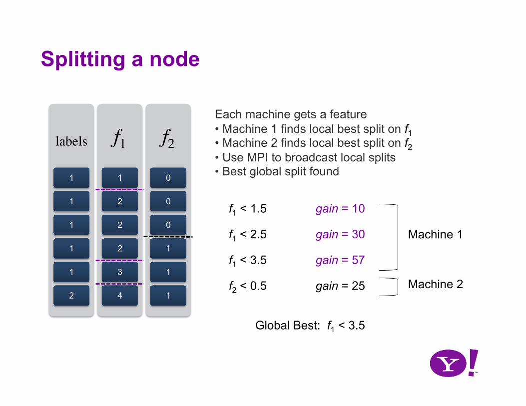
Each machine gets a feature • Machine 1 finds local best split on f1 • Machine 2 finds local best split on f2 • Use MPI to broadcast local splits • Best global split found
f1 < 1.5
f1 < 2.5
f1 < 3.5
f2 < 0.5
gain = 10
gain = 30
gain = 57
gain = 25
Splitting a node
Machine 1
Machine 2
Global Best: f1 < 3.5
f1 1
2
2
2
3
4
f2 0
0
0
1
1
1
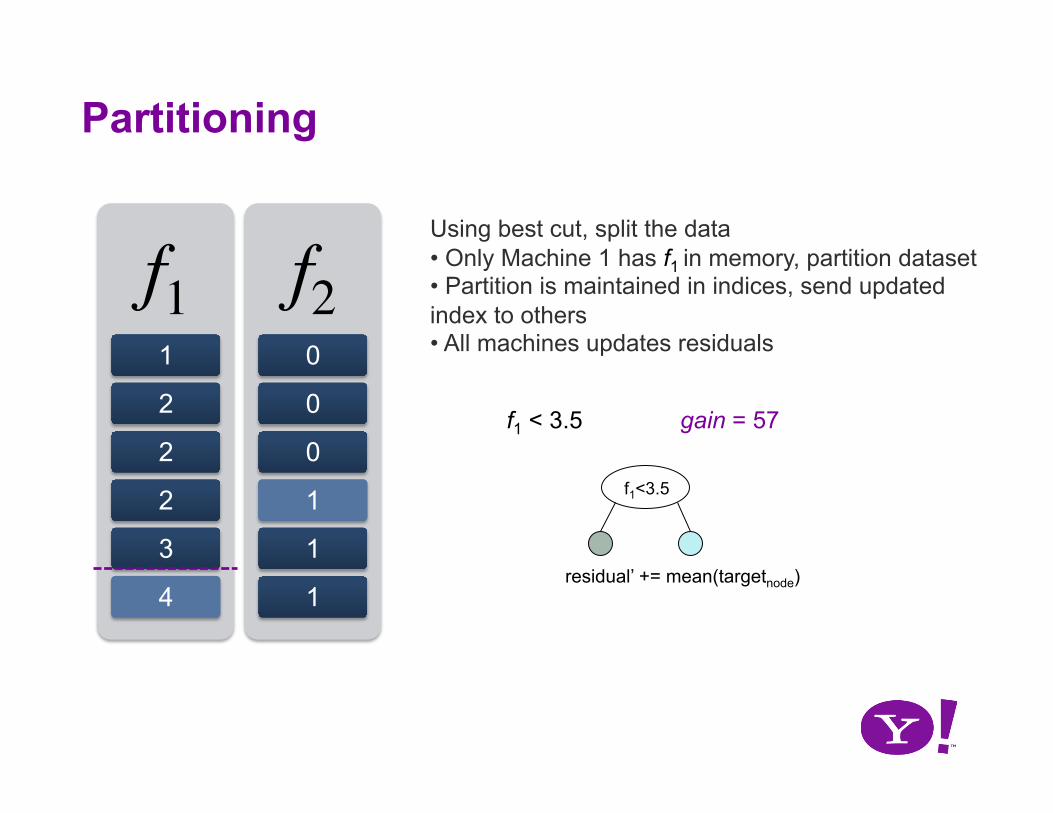
Using best cut, split the data • Only Machine 1 has f1 in memory, partition dataset • Partition is maintained in indices, send updated index to others • All machines updates residuals
f1 < 3.5 gain = 57
f1<3.5
residual’ += mean(targetnode)
Partitioning
€
Fm (x) = Fm−1(x) + ν ⋅ γ lm1(x ∈ Rlm )l=1
L∑
gradientm+1(x) = label(x) − Fm (x)
labels 1
1
1
1
1
2
• Scores are kept for all samples through training of trees • All machines computes new gradients and updates targets for next tree • Repeat until finished
+
Boosting

Experiments
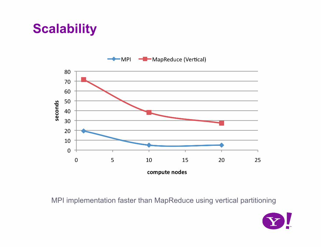
Scalability
MPI implementation faster than MapReduce using vertical partitioning
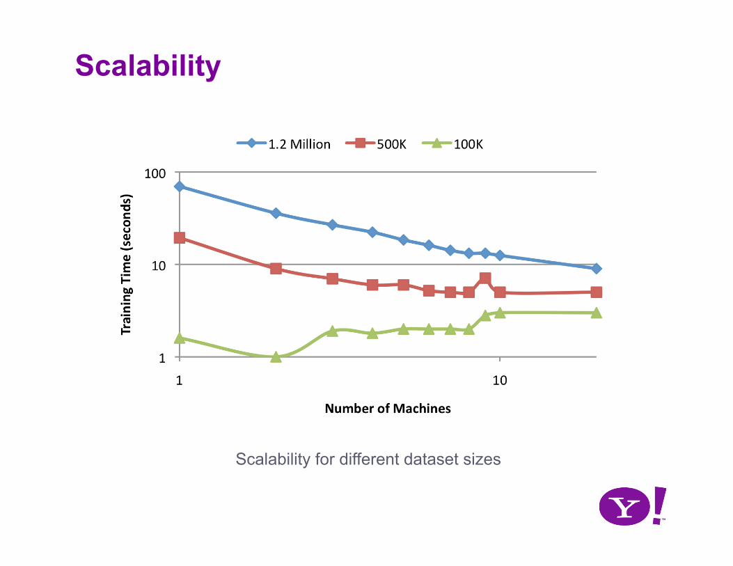
Scalability
Scalability for different dataset sizes
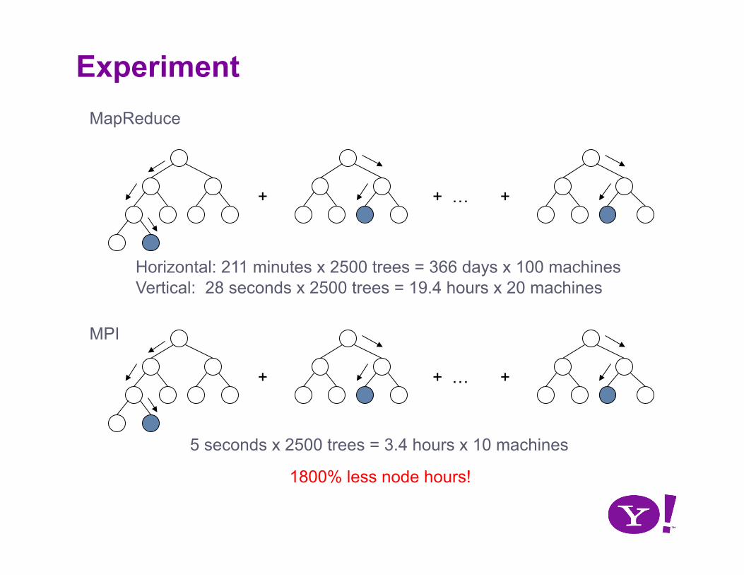
Experiment
+ + + …
+ + + …
Horizontal: 211 minutes x 2500 trees = 366 days x 100 machines Vertical: 28 seconds x 2500 trees = 19.4 hours x 20 machines
5 seconds x 2500 trees = 3.4 hours x 10 machines
1800% less node hours!
MapReduce
MPI
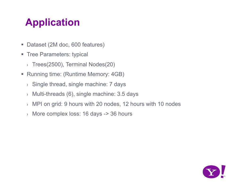
Application
Dataset (2M doc, 600 features)
Tree Parameters: typical
› Trees(2500), Terminal Nodes(20)
Running time: (Runtime Memory: 4GB)
› Single thread, single machine: 7 days
› Multi-threads (6), single machine: 3.5 days
› MPI on grid: 9 hours with 20 nodes, 12 hours with 10 nodes
› More complex loss: 16 days -> 36 hours
Conclusions
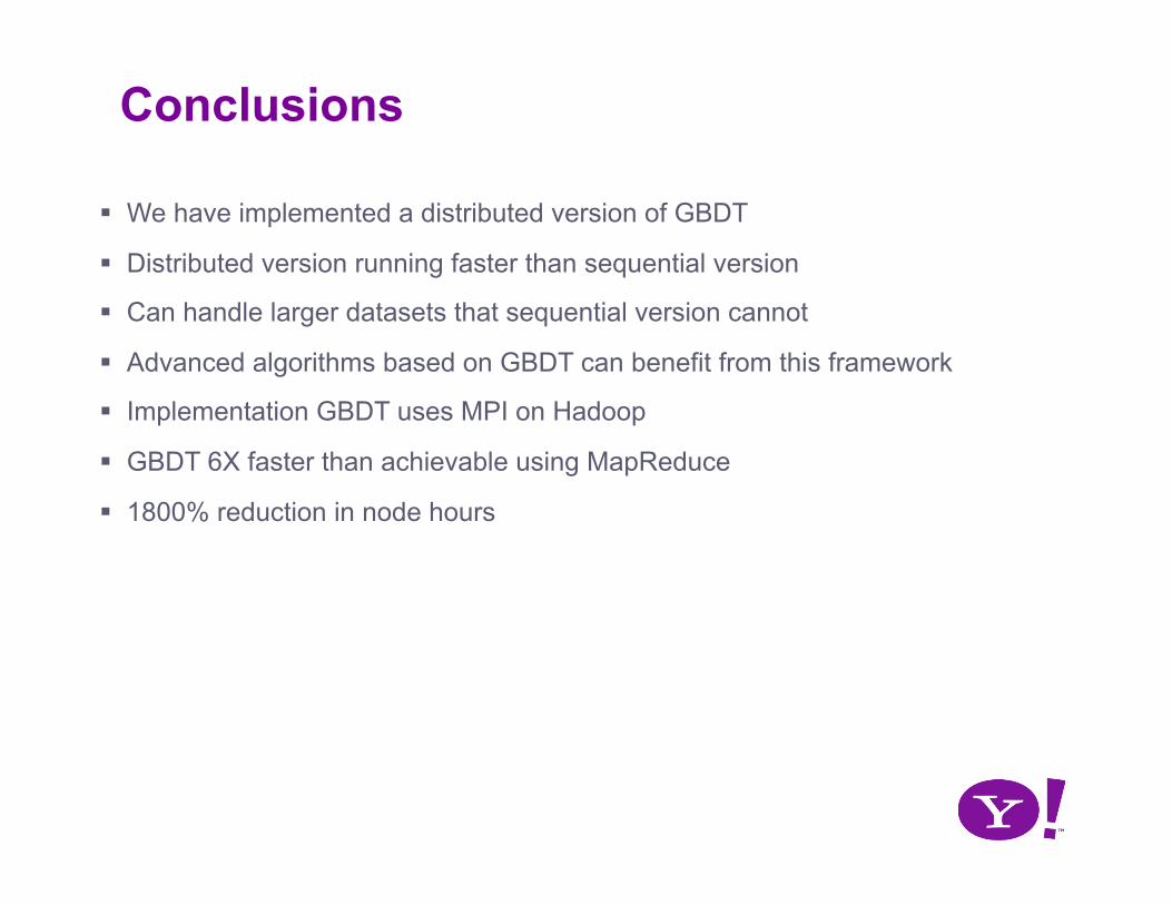
We have implemented a distributed version of GBDT
Distributed version running faster than sequential version
Can handle larger datasets that sequential version cannot
Advanced algorithms based on GBDT can benefit from this framework
Implementation GBDT uses MPI on Hadoop
GBDT 6X faster than achievable using MapReduce
1800% reduction in node hours

Thanks! For more info: [email protected]
References 1 AMDAHL, G. Validity of the single processor approach to
achieving large-scale computing capabilities. pp. 483–485.
2 CARAGEA, D., SILVESCU, A., AND HONAVAR, V. A framework for learning from distributed data using sufficient statistics and its application to learning decision trees. International Journal of Hybrid Intelligent Systems 1, 2 (2004).
3 CHEN, K., LU, R., WONG, C. K., SUN, G., HECK, L., AND TSENG, B. L. Trada: tree based ranking function adaptation. In CIKM (2008), pp. 1143–1152.
4 DEAN, J., AND GHEMAWAT, S. Mapreduce: simplified data processing on large clusters. Commun. ACM 51, 1 (2008), 107–113.
5 FOUNDATION, A. Apache hadoop project. lucene.apache.org/hadoop.
6 FRIEDMAN, J. H. Greedy function approximation: A gradient boosting machine. Annals of Statistics 29 (2001), 1189–1232.
7 FRIEDMAN, J. H. Stochastic gradient boosting. Comput. Stat. Data Anal. 38, 4 (February 2002), 367–378.
8 GEHRKE, J., RAMAKRISHNAN, R., AND GANTI, V. Rainforest - a framework for fast decision tree construction of large datasets. In VLDB’98, Proceedings of 24rd International Conference on Very Large Data Bases, August 24-27, 1998, New York City, New York, USA (1998), A. Gupta, O. Shmueli, and J. Widom, Eds., Morgan Kaufmann, pp. 416–427.
9 GRAHAM, R. L., AND GRAHAMT, R. L. Bounds on multiprocessing timing anomalies. SIAM Journal on Applied Mathematics 17 (1969), 416–429.
10 PANDA, B., HERBACH, J. S., BASU, S., AND BAYARDO, R. J. Planet: Massively parallel learning of tree ensembles. In VLDB 2009, Proceedings of the 35th Int’l Conf. on Very Large Data Bases (2009).
11 PROVOST, F., KOLLURI, V., AND FAYYAD, U. A survey of methods for scaling up inductive algorithms. Data Mining and Knowledge Discovery 3 (1999), 131–169.
12 QUINLAN, J. R. Induction of decision trees. In Machine Learning (1986), pp. 81–106.
13 SHAFER, J. C., AGRAWAL, R., AND 0002, M. M. Sprint: A scalable parallel classifier for data mining. In VLDB’96, Proceedings of 22th International Conference on Very Large Data Bases, September 3-6, 1996, Mumbai (Bombay), India (1996), T. M. Vijayaraman, A. P. Buchmann, C. Mohan, and N. L. Sarda, Eds., Morgan Kaufmann, pp. 544–555.
14 STATISTICS, L. B., AND BREIMAN, L. Random forests. In Machine Learning (2001), pp. 5–32.
15 SU, J., AND ZHANG, H. A fast decision tree learning algorithm. In AAAI (2006).
16 ZHENG, Z., CHEN, K., SUN, G., AND ZHA, H. A regression framework for learning ranking functions using relative relevance judgments. Proceedings of the 30th annual international ACM SIGIR conference on Research and development in information retrieval (2007), 287–294.
Top Related