Download - GPU Implementation of Fully Constrained Linear Spectral ... · GPU Implementation of Fully Constrained Linear Spectral Unmixing for Remotely Sensed Hyperspectral Data Exploitation

GPU Implementation of Fully Constrained Linear Spectral

Unmixing for Remotely Sensed Hyperspectral Data

Exploitation

Sergio Sancheza, Gabriel Martına, Antonio Plazaa and Chein-I Changb

aHyperspectral Computing LaboratoryDepartment of Technology of Computers and Communications

University of Extremadura, Avda. de la Universidad s/n10071 Caceres, Spain

bRemote Sensing Signal and Image Processing LaboratoryDepartment of Computer Science and Electrical Engineering

University of Maryland, Baltimore County1000 Hilltop Circle, Baltimore, MD 21250, USA

ABSTRACT

Spectral unmixing is an important task for remotely sensed hyperspectral data exploitation. The spectral signa-tures collected in natural environments are invariably a mixture of the pure signatures of the various materialsfound within the spatial extent of the ground instantaneous field view of the imaging instrument. Spectralunmixing aims at inferring such pure spectral signatures, called endmembers, and the material fractions, calledfractional abundances, at each pixel of the scene. A standard technique for spectral mixture analysis is linearspectral unmixing, which assumes that the collected spectra at the spectrometer can be expressed in the formof a linear combination of endmembers weighted by their corresponding abundances, expected to obey two con-straints, i.e. all abundances should be non-negative, and the sum of abundances for a given pixel should beunity. Several techniques have been developed in the literature for unconstrained, partially constrained and fullyconstrained linear spectral unmixing, which can be computationally expensive (in particular, for complex high-dimensional scenes with a high number of endmembers). In this paper, we develop new parallel implementationsof unconstrained, partially constrained and fully constrained linear spectral unmixing algorithms. The imple-mentations have been developed in programmable graphics processing units (GPUs), an exciting developmentin the field of commodity computing that fits very well the requirements of on-board data processing scenarios,in which low-weight and low-power integrated components are mandatory to reduce mission payload. Our ex-periments, conducted with a hyperspectral scene collected over the World Trade Center area in New York City,indicate that the proposed implementations provide relevant speedups over the corresponding serial versions inlatest-generation Tesla C1060 GPU architectures.

Keywords: Hyperspectral imaging, spectral unmixing, parallel computing, graphics processing units (GPUs).

1. INTRODUCTION

Spectral mixture analysis (also called spectral unmixing) has been an alluring exploitation goal from the earliestdays of hyperspectral imaging1 to our days.2, 3 No matter the spatial resolution, the spectral signatures collectedin natural environments are invariably a mixture of the signatures of the various materials found within thespatial extent of the ground instantaneous field view of the imaging instrument.4 For instance, it is likely thatthe pixel collected over a vegetation area in Fig. 1 actually comprises a mixture of vegetation and soil. In thiscase, the measured spectrum may be decomposed into a combination of pure spectral signatures of soil andvegetation, weighted by areal coefficients that indicate the proportion of each macroscopically pure signaturein the mixed pixel.5 The availability of hyperspectral imagers with a number of spectral bands that exceeds

Send correspondence to Antonio J. Plaza:E-mail: [email protected]; Telephone: +34 927 257000 (Ext. 51662); URL: http://www.umbc.edu/rssipl/people/aplaza

Satellite Data Compression, Communications, and Processing VI, edited by Bormin Huang, Antonio J. Plaza, Joan Serra-Sagristà, Chulhee Lee, Yunsong Li, Shen-En Qian, Proc. of SPIE Vol. 7810, 78100G

© 2010 SPIE · CCC code: 0277-786X/10/$18 · doi: 10.1117/12.860775

Proc. of SPIE Vol. 7810 78100G-1

Downloaded from SPIE Digital Library on 09 Sep 2010 to 158.42.236.149. Terms of Use: http://spiedl.org/terms

Figure 1. The mixture problem in remotely sensed hyperspectral data analysis.

Figure 2. Linear versus nonlinear mixture models: single versus multiple scattering.

the number of spectral mixture components6 has allowed to cast the unmixing problem in terms of an over-determined system of equations in which, given a set of pure spectral signatures (called endmembers) the actualunmixing to determine apparent pixel abundance fractions can be defined in terms of a numerical inversionprocess.7

A standard technique for spectral mixture analysis is linear spectral unmixing,8, 9 which assumes that thecollected spectra at the spectrometer can be expressed in the form of a linear combination of endmembersweighted by their corresponding abundances. It should be noted that the linear mixture model assumes minimalsecondary reflections and/or multiple scattering effects in the data collection procedure, and hence the measuredspectra can be expressed as a linear combination of the spectral signatures of materials present in the mixed pixel[see Fig. 2(a)]. Although the linear model has practical advantages such as ease of implementation and flexibilityin different applications,10 nonlinear spectral unmixing may best characterize the resultant mixed spectra forcertain endmember distributions, such as those in which the endmember components are randomly distributedthroughout the field of view of the instrument.11, 12 In those cases, the mixed spectra collected at the imaginginstrument is better described by assuming that part of the source radiation is multiply scattered before beingcollected at the sensor [see Fig. 2(b)].

Although linear spectral unmixing is generally more tractable in computational terms than nonlinear unmix-ing, it is still a quite computationally expensive process due to the extremely high dimensionality of hyperspectraldata cubes. Solving the mixture model generally involves: 1) identifying a collection of endmembers in the im-age, and 2) estimating their abundance in each pixel. The standard hyperspectral unmixing chain is graphicallyillustrated by a flowchart in Figure 3. In our work, we do not include the dimensionality reduction step in Fig.3, which is mainly intended to reduce processing time but often discards relevant information in the spectral



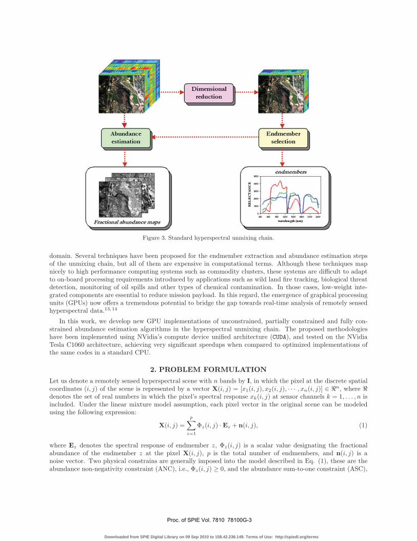
Figure 3. Standard hyperspectral unmixing chain.

domain. Several techniques have been proposed for the endmember extraction and abundance estimation stepsof the unmixing chain, but all of them are expensive in computational terms. Although these techniques mapnicely to high performance computing systems such as commodity clusters, these systems are difficult to adaptto on-board processing requirements introduced by applications such as wild land fire tracking, biological threatdetection, monitoring of oil spills and other types of chemical contamination. In those cases, low-weight inte-grated components are essential to reduce mission payload. In this regard, the emergence of graphical processingunits (GPUs) now offers a tremendous potential to bridge the gap towards real-time analysis of remotely sensedhyperspectral data.13, 14

In this work, we develop new GPU implementations of unconstrained, partially constrained and fully con-strained abundance estimation algorithms in the hyperspectral unmixing chain. The proposed methodologieshave been implemented using NVidia’s compute device unified architecture (CUDA), and tested on the NVidiaTesla C1060 architecture, achieving very significant speedups when compared to optimized implementations ofthe same codes in a standard CPU.

2. PROBLEM FORMULATION

Let us denote a remotely sensed hyperspectral scene with n bands by I, in which the pixel at the discrete spatialcoordinates (i, j) of the scene is represented by a vector X(i, j) = [x1(i, j), x2(i, j), · · · , xn(i, j)] ∈ �n, where �denotes the set of real numbers in which the pixel’s spectral response xk(i, j) at sensor channels k = 1, . . . , n isincluded. Under the linear mixture model assumption, each pixel vector in the original scene can be modeledusing the following expression:

X(i, j) =

p∑z=1

Φz(i, j) · Ez + n(i, j), (1)

where Ez denotes the spectral response of endmember z, Φz(i, j) is a scalar value designating the fractionalabundance of the endmember z at the pixel X(i, j), p is the total number of endmembers, and n(i, j) is anoise vector. Two physical constrains are generally imposed into the model described in Eq. (1), these are theabundance non-negativity constraint (ANC), i.e., Φz(i, j) ≥ 0, and the abundance sum-to-one constraint (ASC),



i.e.,∑p

z=1 Φz(i, j) = 1.8 Once a set of endmembers E = {Ez}pz=1 have been extracted by a certain algorithm,9

their correspondent abundance fractions Φ(i, j) = {Φz(i, j)}pz=1 in a specific pixel vector X(i, j) of the image I

can be estimated (in least squares sense) by the following unconstrained expression:10

ΦLSU(i, j) = (ETE)−1ETX(i, j). (2)

However, it should be noted that the fractional abundance estimations obtained by means of Eq. (2) do not satisfythe ASC and ANC constraints. Imposing the ASC constraint results in the following optimization problem:

minΦ(i,j)∈Δ

{(X(i, j) − Φ(i, j) ·E)

T(X(i, j) − Φ(i, j) ·E)

},

subject to: Δ =

{Φ(i, j)

⏐⏐⏐⏐⏐p∑

z=1

Φz(i, j) = 1

}. (3)

Similarly, imposing the ANC constraint results in the following optimization problem:

minΦ(i,j)∈Δ

{(X(i, j) − Φ(i, j) ·E)T (X(i, j) − Φ(i, j) ·E)

},

subject to: Δ = {Φ(i, j)|Φz(i, j) ≥ 0 for all 1 ≤ z ≤ p} . (4)

As indicated in previous work,8, 15 a non-negative constrained least squares (NCLS) algorithm can be used toobtain a solution to the ANC-constrained problem described in Eq. (4) in iterative fashion.16 In order to takecare of the ASC constraint, a new endmember signature matrix, denoted by E′, and a modified version of thepixel vector X(i, j), denoted by X′(i, j), are introduced as follows:

E′ =

[δM

1T

], Φ′(i, j) =

[δΦ(i, j)

1

], (5)

where 1 = (1, 1, · · · , 1︸︷︷︸p

)T and δ controls the impact of the ASC constraint. Using the two expressions in (5), a

fully constrained estimate can be directly obtained from the NCLS algorithm by replacing E and Φ(i, j) used inthe NCLS algorithm with E′ and Φ′(i, j). This fully constrained (i.e. ASC-constrained and ANC-constrained)linear spectral unmixing estimate is referred to by the acronym FCLSU.8

3. GPU IMPLEMENTATIONS

This section describes our GPU implementations of abundance estimation algorithms. GPUs can be abstractedin terms of a stream model, under which all data sets are represented as streams (i.e., ordered data sets).Algorithms are constructed by chaining so-called kernels, which operate on entire streams, taking one or morestreams as inputs and producing one or more streams as outputs.13 Thereby, data-level parallelism is exposed tohardware, and kernels can be concurrently applied. First, we present a GPU implementation of the unconstrainedunmixing method, called GPU-LSU. Then, we describe our parallel version of the NCLS algorithm, called GPU-NCLS. Finally, we describe the parallel version of FCLSU which is referred to as GPU-FCLSU. In all cases,code examples illustrating the most relevant kernels constructed in the GPU implementations are given to betterunderstand our designs.



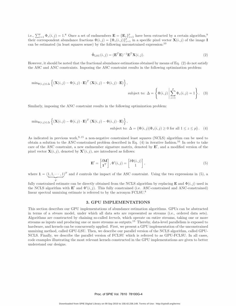
Figure 4. CUDA kernel Unmixing that computes unconstrained abundances in each pixel of the hyperspectral image.

3.1 GPU-LSU

Our GPU version of the unconstrained abundance estimation algorithm assumes that a set of endmembersis available and produces a set of endmember abundance maps as follows. The first step in the GPU-LSU

is to calculate a so-called compute matrix(ETE

)−1

ET , where E = {Ez}pz=1 is formed by the p endmembers

previously extracted. This compute matrix will be multiplied by all pixel vectors X(i, j) in the original image. Inour implementation, the compute matrix is calculated in the CPU mainly due to two reasons: 1) its computationis relatively fast, and 2) once calculated, the compute matrix remains the same throughout the whole execution ofthe code. The compute matrix is now multiplied by each pixel X(i, j) in the hyperspectral image, thus obtaininga set of abundance vectors Φ(i, j), each containing the fractional abundances of the p endmembers in each pixel.This is accomplished in the GPU by means of the Unmixing kernel illustrated in Fig. 4, in which the outcomeof the unmixing process (i.e. the p endmember abundance maps) are stored in d image unmixed.

3.2 GPU-NCLS and GPU-FCLSU

Our GPU version of the ANC-constrained abundance estimation algorithm (called GPU-NCLS) is approachedfrom the perspective of a distance minimization problem where the distance between the measured pixel orspectra and the estimate is the smallest. For this purpose, we resort to the image space reconstruction algorithm(ISRA),15 an iterative algorithm and an example of an algorithm satisfying only the ANC constraint. In otherwords, this algorithm guarantees convergence in a finite number of iterations and positive values in the abundanceestimation results for any input set of endmembers. For illustrative purposes, Fig. 5 shows the ISRA kernel,which iteratively calculates the fractional abundance of a set of pre-calculated endmembers Ez in a pixel X(i, j)independently of the other pixels and, hence, can be efficiently executed in parallel. Finally, Fig. 6 shows thekernel used to implement the GPU-FCLSU algorithm. This kernel simply scales the abundances provided byGPU-NCLS to provide fully constrained estimates.



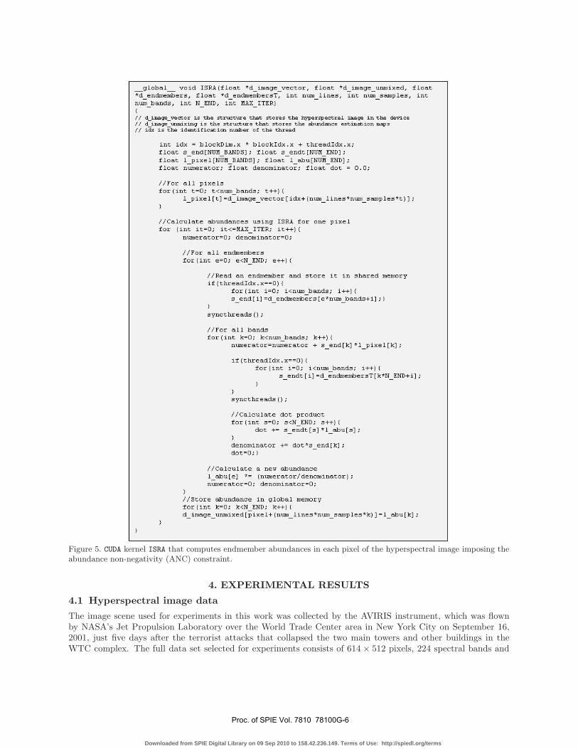
Figure 5. CUDA kernel ISRA that computes endmember abundances in each pixel of the hyperspectral image imposing theabundance non-negativity (ANC) constraint.

4. EXPERIMENTAL RESULTS

4.1 Hyperspectral image data

The image scene used for experiments in this work was collected by the AVIRIS instrument, which was flownby NASA’s Jet Propulsion Laboratory over the World Trade Center area in New York City on September 16,2001, just five days after the terrorist attacks that collapsed the two main towers and other buildings in theWTC complex. The full data set selected for experiments consists of 614 × 512 pixels, 224 spectral bands and



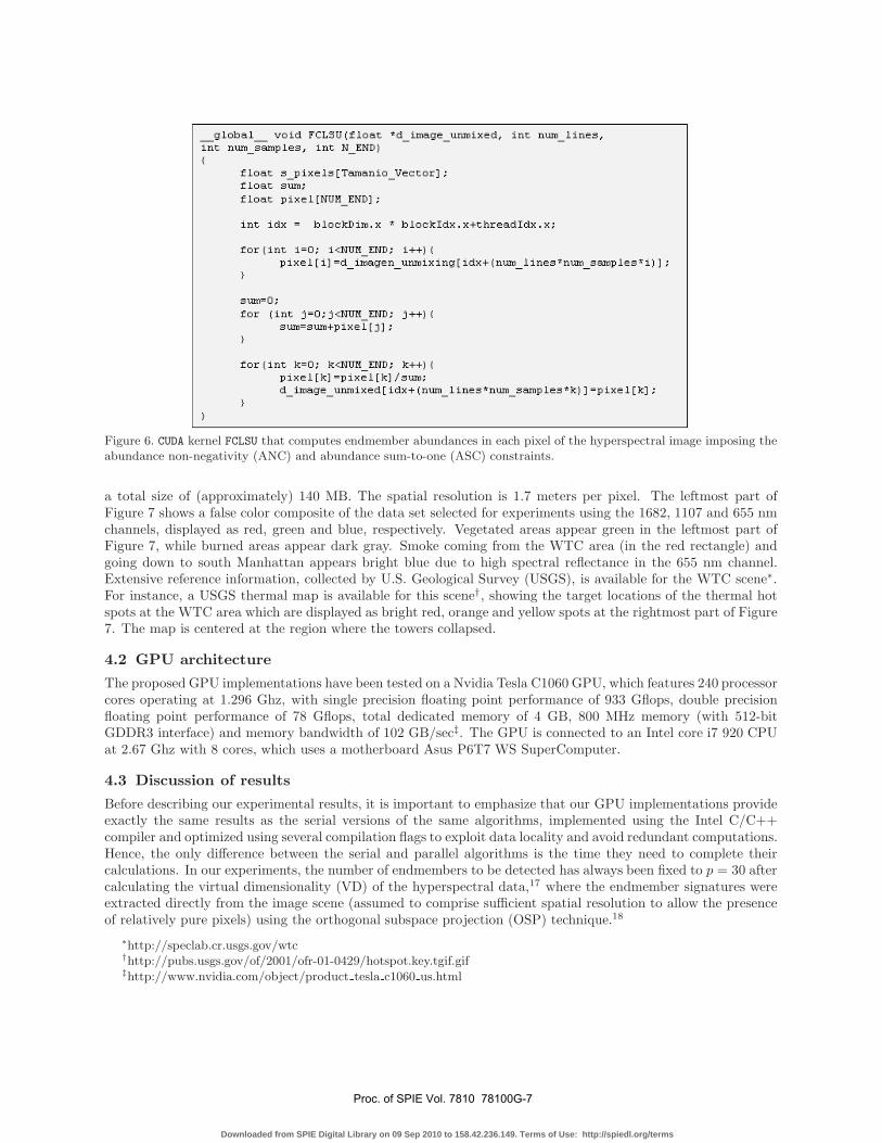
Figure 6. CUDA kernel FCLSU that computes endmember abundances in each pixel of the hyperspectral image imposing theabundance non-negativity (ANC) and abundance sum-to-one (ASC) constraints.

a total size of (approximately) 140 MB. The spatial resolution is 1.7 meters per pixel. The leftmost part ofFigure 7 shows a false color composite of the data set selected for experiments using the 1682, 1107 and 655 nmchannels, displayed as red, green and blue, respectively. Vegetated areas appear green in the leftmost part ofFigure 7, while burned areas appear dark gray. Smoke coming from the WTC area (in the red rectangle) andgoing down to south Manhattan appears bright blue due to high spectral reflectance in the 655 nm channel.Extensive reference information, collected by U.S. Geological Survey (USGS), is available for the WTC scene∗.For instance, a USGS thermal map is available for this scene†, showing the target locations of the thermal hotspots at the WTC area which are displayed as bright red, orange and yellow spots at the rightmost part of Figure7. The map is centered at the region where the towers collapsed.

4.2 GPU architecture

The proposed GPU implementations have been tested on a Nvidia Tesla C1060 GPU, which features 240 processorcores operating at 1.296 Ghz, with single precision floating point performance of 933 Gflops, double precisionfloating point performance of 78 Gflops, total dedicated memory of 4 GB, 800 MHz memory (with 512-bitGDDR3 interface) and memory bandwidth of 102 GB/sec‡. The GPU is connected to an Intel core i7 920 CPUat 2.67 Ghz with 8 cores, which uses a motherboard Asus P6T7 WS SuperComputer.

4.3 Discussion of results

Before describing our experimental results, it is important to emphasize that our GPU implementations provideexactly the same results as the serial versions of the same algorithms, implemented using the Intel C/C++compiler and optimized using several compilation flags to exploit data locality and avoid redundant computations.Hence, the only difference between the serial and parallel algorithms is the time they need to complete theircalculations. In our experiments, the number of endmembers to be detected has always been fixed to p = 30 aftercalculating the virtual dimensionality (VD) of the hyperspectral data,17 where the endmember signatures wereextracted directly from the image scene (assumed to comprise sufficient spatial resolution to allow the presenceof relatively pure pixels) using the orthogonal subspace projection (OSP) technique.18

∗http://speclab.cr.usgs.gov/wtc†http://pubs.usgs.gov/of/2001/ofr-01-0429/hotspot.key.tgif.gif‡http://www.nvidia.com/object/product tesla c1060 us.html



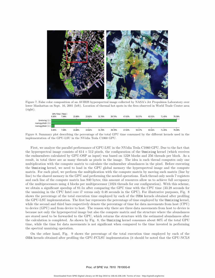
Figure 7. False color composition of an AVIRIS hyperspectral image collected by NASA’s Jet Propulsion Laboratory overlower Manhattan on Sept. 16, 2001 (left). Location of thermal hot spots in the fires observed in World Trade Center area(right).

Figure 8. Summary plot describing the percentage of the total GPU time consumed by the different kernels used in theimplementation of the GPU-LSU in the NVidia Tesla C1060 GPU.

First, we analyze the parallel performance of GPU-LSU in the NVidia Tesla C1060 GPU. Due to the fact thatthe hyperspectral image consists of 614 × 512 pixels, the configuration of the Unmixing kernel (which receivesthe endmembers calculated by GPU-OSP as input) was based on 1228 blocks and 256 threads per block. As aresult, in total there are as many threads as pixels in the image. The idea is each thread computes only onemultiplication with the compute matrix to calculate the endmember abundances in the pixel. Before executingthe Unmixing kernel, we need to load in the GPU global memory the hyperspectral image and the computematrix. For each pixel, we perform the multiplication with the compute matrix by moving such matrix (line byline) to the shared memory in the GPU and performing the needed operations. Each thread only needs 7 registersand each line of the compute matrix has 940 bytes; this amount of resources allow us to achieve full occupancyof the multiprocessors using 4 blocks per multiprocessor (1024 threads for our configuration). With this scheme,we obtain a significant speedup of 81.5x after comparing the GPU time with the CPU time (33.28 seconds forthe unmixing in the CPU Intel core i7 versus only 0.48 seconds in the GPU). For illustrative purposes, Fig. 8shows the percentage of the total execution time employed by each of the CUDA kernels obtained after profilingthe GPU-LSU implementation. The first bar represents the percentage of time employed by the Unmixing kernel,while the second and third bars respectively denote the percentage of time for data movements from host (CPU)to device (GPU) and from device to host. The reason why there are three data movements from host to device isbecause not only the hyperspectral image but also the compute matrix and the structure where the abundancesare stored need to be forwarded to the GPU, which returns the structure with the estimated abundances afterthe calculation is completed. As shown by Fig. 8, the Unmixing kernel consumes about 80% of the total GPUtime, while the time for data movements is not significant when compared to the time invested in performingthe spectral unmixing operation.

On the other hand, Fig. 9 shows the percentage of the total execution time employed by each of theCUDA kernels obtained after profiling the GPU-FCLSU implementation (it should be noted that the GPU-NCLS



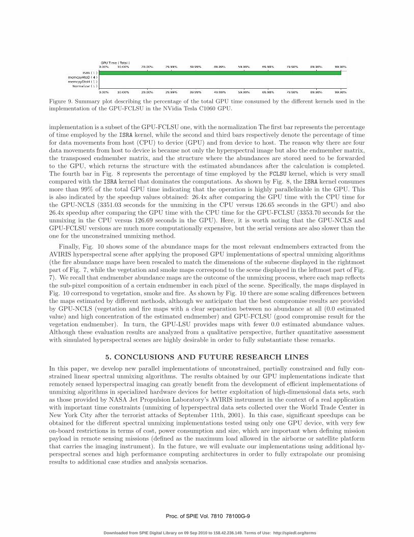
Figure 9. Summary plot describing the percentage of the total GPU time consumed by the different kernels used in theimplementation of the GPU-FCLSU in the NVidia Tesla C1060 GPU.

implementation is a subset of the GPU-FCLSU one, with the normalization The first bar represents the percentageof time employed by the ISRA kernel, while the second and third bars respectively denote the percentage of timefor data movements from host (CPU) to device (GPU) and from device to host. The reason why there are fourdata movements from host to device is because not only the hyperspectral image but also the endmember matrix,the transposed endmember matrix, and the structure where the abundances are stored need to be forwardedto the GPU, which returns the structure with the estimated abundances after the calculation is completed.The fourth bar in Fig. 8 represents the percentage of time employed by the FCLSU kernel, which is very smallcompared with the ISRA kernel that dominates the computations. As shown by Fig. 8, the ISRA kernel consumesmore than 99% of the total GPU time indicating that the operation is highly parallelizable in the GPU. Thisis also indicated by the speedup values obtained: 26.4x after comparing the GPU time with the CPU time forthe GPU-NCLS (3351.03 seconds for the unmixing in the CPU versus 126.65 seconds in the GPU) and also26.4x speedup after comparing the GPU time with the CPU time for the GPU-FCLSU (3353.70 seconds for theunmixing in the CPU versus 126.69 seconds in the GPU). Here, it is worth noting that the GPU-NCLS andGPU-FCLSU versions are much more computationally expensive, but the serial versions are also slower than theone for the unconstrained unmixing method.

Finally, Fig. 10 shows some of the abundance maps for the most relevant endmembers extracted from theAVIRIS hyperspectral scene after applying the proposed GPU implementations of spectral unmixing algorithms(the fire abundance maps have been rescaled to match the dimensions of the subscene displayed in the rightmostpart of Fig. 7, while the vegetation and smoke maps correspond to the scene displayed in the leftmost part of Fig.7). We recall that endmember abundance maps are the outcome of the unmixing process, where each map reflectsthe sub-pixel composition of a certain endmember in each pixel of the scene. Specifically, the maps displayed inFig. 10 correspond to vegetation, smoke and fire. As shown by Fig. 10 there are some scaling differences betweenthe maps estimated by different methods, although we anticipate that the best compromise results are providedby GPU-NCLS (vegetation and fire maps with a clear separation between no abundance at all (0.0 estimatedvalue) and high concentration of the estimated endmember) and GPU-FCLSU (good compromise result for thevegetation endmember). In turn, the GPU-LSU provides maps with fewer 0.0 estimated abundance values.Although these evaluation results are analyzed from a qualitative perspective, further quantitative assessmentwith simulated hyperspectral scenes are highly desirable in order to fully substantiate these remarks.

5. CONCLUSIONS AND FUTURE RESEARCH LINES

In this paper, we develop new parallel implementations of unconstrained, partially constrained and fully con-strained linear spectral unmixing algorithms. The results obtained by our GPU implementations indicate thatremotely sensed hyperspectral imaging can greatly benefit from the development of efficient implementations ofunmixing algorithms in specialized hardware devices for better exploitation of high-dimensional data sets, suchas those provided by NASA Jet Propulsion Laboratory’s AVIRIS instrument in the context of a real applicationwith important time constraints (unmixing of hyperspectral data sets collected over the World Trade Center inNew York City after the terrorist attacks of September 11th, 2001). In this case, significant speedups can beobtained for the different spectral unmixing implementations tested using only one GPU device, with very fewon-board restrictions in terms of cost, power consumption and size, which are important when defining missionpayload in remote sensing missions (defined as the maximum load allowed in the airborne or satellite platformthat carries the imaging instrument). In the future, we will evaluate our implementations using additional hy-perspectral scenes and high performance computing architectures in order to fully extrapolate our promisingresults to additional case studies and analysis scenarios.



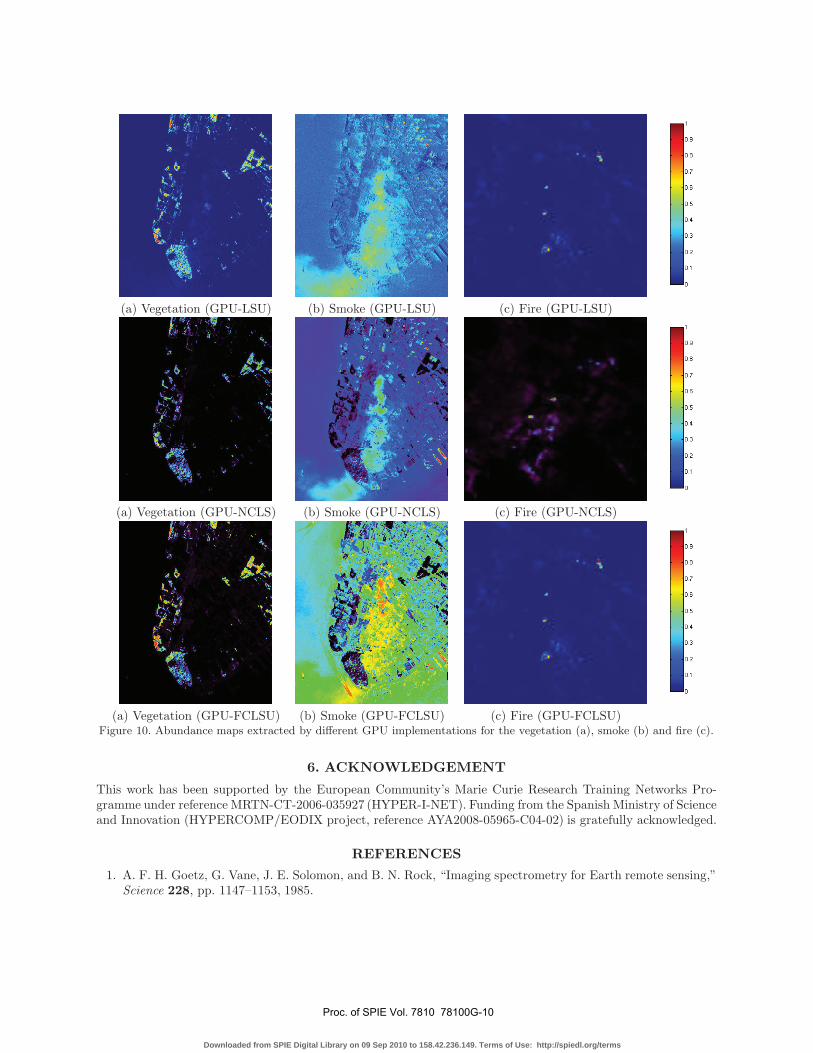
(a) Vegetation (GPU-LSU) (b) Smoke (GPU-LSU) (c) Fire (GPU-LSU)

(a) Vegetation (GPU-NCLS) (b) Smoke (GPU-NCLS) (c) Fire (GPU-NCLS)

(a) Vegetation (GPU-FCLSU) (b) Smoke (GPU-FCLSU) (c) Fire (GPU-FCLSU)Figure 10. Abundance maps extracted by different GPU implementations for the vegetation (a), smoke (b) and fire (c).

6. ACKNOWLEDGEMENT

This work has been supported by the European Community’s Marie Curie Research Training Networks Pro-gramme under reference MRTN-CT-2006-035927 (HYPER-I-NET). Funding from the Spanish Ministry of Scienceand Innovation (HYPERCOMP/EODIX project, reference AYA2008-05965-C04-02) is gratefully acknowledged.

REFERENCES

1. A. F. H. Goetz, G. Vane, J. E. Solomon, and B. N. Rock, “Imaging spectrometry for Earth remote sensing,”Science 228, pp. 1147–1153, 1985.



2. A. Plaza, J. A. Benediktsson, J. Boardman, J. Brazile, L. Bruzzone, G. Camps-Valls, J. Chanussot, M. Fau-vel, P. Gamba, J. Gualtieri, M. Marconcini, J. C. Tilton, and G. Trianni, “Recent advances in techniquesfor hyperspectral image processing,” Remote Sensing of Environment 113, pp. 110–122, 2009.

3. M. E. Schaepman, S. L. Ustin, A. Plaza, T. H. Painter, J. Verrelst, and S. Liang, “Earth system sciencerelated imaging spectroscopy – an assessment,” Remote Sensing of Environment 113, pp. 123–137, 2009.

4. J. B. Adams, M. O. Smith, and P. E. Johnson, “Spectral mixture modeling: a new analysis of rock and soiltypes at the Viking Lander 1 site,” Journal of Geophysical Research 91, pp. 8098–8112, 1986.

5. N. Keshava and J. F. Mustard, “Spectral unmixing,” IEEE Signal Processing Magazine 19(1), pp. 44–57,2002.

6. R. O. Green, M. L. Eastwood, C. M. Sarture, T. G. Chrien, M. Aronsson, B. J. Chippendale, J. A. Faust,B. E. Pavri, C. J. Chovit, M. Solis, et al., “Imaging spectroscopy and the airborne visible/infrared imagingspectrometer (AVIRIS),” Remote Sensing of Environment 65(3), pp. 227–248, 1998.

7. J. E. Ball, L. M. Bruce, and N. Younan, “Hyperspectral pixel unmixing via spectral band selection and dc-insensitive singular value decomposition,” IEEE Geoscience and Remote Sensing Letters 4(3), pp. 382–386,2007.

8. D. Heinz and C.-I. Chang, “Fully constrained least squares linear mixture analysis for material quantificationin hyperspectral imagery,” IEEE Transactions on Geoscience and Remote Sensing 39, pp. 529–545, 2001.

9. A. Plaza, P. Martinez, R. Perez, and J. Plaza, “A quantitative and comparative analysis of endmember ex-traction algorithms from hyperspectral data,” IEEE Transactions on Geoscience and Remote Sensing 42(3),pp. 650–663, 2004.

10. C.-I. Chang, Hyperspectral Imaging: Techniques for Spectral Detection and Classification, Kluwer Aca-demic/Plenum Publishers: New York, 2003.

11. K. J. Guilfoyle, M. L. Althouse, and C.-I. Chang, “A quantitative and comparative analysis of linear andnonlinear spectral mixture models using radial basis function neural networks,” IEEE Trans. Geosci. Remote

Sens. 39, pp. 2314–2318, 2001.

12. J. Plaza, A. Plaza, R. Perez, and P. Martinez, “On the use of small training sets for neural network-based characterization of mixed pixels in remotely sensed hyperspectral images,” Pattern Recognition 42,pp. 3032–3045, 2009.

13. J. Setoain, M. Prieto, C. Tenllado, A. Plaza, and F. Tirado, “Parallel morphological endmember extractionusing commodity graphics hardware,” IEEE Geoscience and Remote Sensing Letters 43, pp. 441–445, 2007.

14. Y. Tarabalka, T. V. Haavardsholm, I. Kasen, and T. Skauli, “Real-time anomaly detection in hyperspec-tral images using multivariate normal mixture models and gpu processing,” Journal of Real-Time Image

Processing 4, pp. 1–14, 2009.

15. A. R. D. Pierro, “On the relation between ISRA and the EM algorithm for positron emission tomography,”IEEE Transactions on Medical Imaging 12, pp. 328–333, 1993.

16. C.-I. Chang and D. Heinz, “Constrained subpixel target detection for remotely sensed imagery,” IEEE

Transactions on Geoscience and Remote Sensing 38, pp. 1144–1159, 2000.

17. C.-I. Chang and Q. Du, “Estimation of number of spectrally distinct signal sources in hyperspectral im-agery,” IEEE Transactions on Geoscience and Remote Sensing 42(3), pp. 608–619, 2004.

18. J. C. Harsanyi and C.-I. Chang, “Hyperspectral image classification and dimensionality reduction: Anorthogonal subspace projection,” IEEE Transactions on Geoscience and Remote Sensing 32(4), pp. 779–785.

