


Languages
Pages
Legal


university ofgroningen
groningen growth anddevelopment centre
GGDC RESEARCH MEMORANDUM 130
Fragmentation, Incomes and Jobs.An analysis of European Competitiveness
Marcel Timmer, Bart Los, Robert Stehrer,Gaaitzen de Vries
May 2013

1
Fragmentation, Incomes and Jobs.
An analysis of European competitiveness
Paper prepared
for the 57th Panel Meeting of Economic Policy, April 2013.
Marcel P. Timmer a,*
Bart Losa
Robert Stehrerb
Gaaitzen de Vriesa
First version Novermber 2012
This version May, 2013
Affiliations a Groningen Growth and Development Centre, Faculty of Economics and Business, University of
Groningen b The Vienna Institute for International Economic Studies (WIIW)
* Corresponding Author
Marcel P. Timmer
Groningen Growth and Development Centre
Faculty of Economics and Business
University of Groningen, The Netherlands
Acknowledgements:
This paper is part of the World Input-Output Database (WIOD) project funded by the European
Commission, Research Directorate General as part of the 7th Framework Programme, Theme 8: Socio-
Economic Sciences and Humanities, grant Agreement no: 225 281. More information on the WIOD-
project can be found at www.wiod.org. We are grateful for the stimulating and useful comments and
suggestions received from many colleagues over the years. Unfortunately, they are too numerous to
enumerate here. Comments from four anonymous referees and the editor Nicola Fuchs-Schündeln are also
gratefully acknowledged.

2
Abstract
Increasing fragmentation of production across borders is changing the nature of international
competition. As a result, conventional indicators of competitiveness based on gross exports
become less informative and new measures are needed. In this paper we propose an ex-post
accounting framework of the value added and workers that are directly and indirectly related to
the production of final manufacturing goods, called ‘manufactures GVC income’ and
‘manufactures GVC jobs’. We outline these concepts and provide trends in European countries
based on a recent multi-sector input-output model of the world economy. We find that since
1995 revealed comparative advantage of the EU27 is shifting to activities related to the
production of non-electrical machinery and transport equipment. The workers involved in
manufactures GVCs are increasingly in services, rather than manufacturing industries. We also
find a strong shift towards activities carried out by high-skilled workers, highlighting the uneven
distributional effects of fragmentation. The results show that a GVC perspective on
competitiveness is needed to better inform the policy debates on globalisation.
NOTE: The main body paper of the paper focuses in particular on trends in the 27 countries
of the European Union. But in an appendix we provide additional results for thirteen other
major countries, including the United States.

3
1. Introduction
The competitiveness of nations is a topic that frequently returns in mass media, governmental
reports and discussions of economic policy. While specific definitions of national
competitiveness are much debated, most economists would agree that the concept refers to a
country’s ability to realise income and employment growth without running into long-run
balance of payments difficulties. The ability of advanced nations to maintain “good jobs” in the
face of rising global competition is a long standing concern. The unleashing of the market
economy in China and India added to global competitive pressures, casually linked to dwindling
manufacturing employment in traditional strongholds in Western Europe, Japan and the US and
curtailing development opportunities for other emerging economies such as in Eastern Europe.
Slow recovery after the global financial crisis in 2008, fuelled demands for more active industrial
policies to restore competitiveness around the world. Rebuilding the competitive strengths of
Europe, and in particular curbing the divergence between Northern and Mediterranean countries,
is therefore high on the European policy agenda.
To track developments in competitiveness, shares in world export markets are
traditionally used as the main indicator. However, this measure is increasingly doubted in a
world with increasing fragmentation of production across borders. Fostered by rapidly falling
communication and coordination costs, the various stages of production need not be performed
near to each other anymore. Increased possibilities for fragmentation mean in essence that more
parts of the production process become open to international competition. In the past
competitiveness of countries was determined by domestic clusters of firms, mainly competing
‘sector to sector’ with other countries, based on the price and quality of their final products. But
globalisation has entered a new phase in which international competition increasingly plays out
at the level of activities within industries, rather than at the level of whole industries, dubbed the
“second unbundling” by Baldwin (2006) (see also Feenstra 1998, 2010). To reflect this change
in the nature of competition, a new measure of competitiveness is needed that is based on the
value added in production by a country, rather than the gross output value of its exports. Or as
put by Grossman and Rossi-Hansberg (2006, p.66-67): “ [But] such measures are inadequate to
the task of measuring the extent of a country’s international integration in a world with global
supply chains…we would like to know the sources of the value added embodied in goods and the
uses to which the goods are eventually put.” In this paper we present a framework which is
developed to do just this. We propose a new measure of the competitiveness of a country based
on value added and jobs involved in global production chains, and show how it can be derived
empirically from a world input-output table.
Concerns about the increasing disconnect between growth in gross exports and the generation of
incomes and jobs for workers have been expressed before. In his analysis of Germany’s
“pathological export boom”, Sinn (2006) suggested that the increasing imports of intermediates,
mainly from Eastern Europe, led to a decline in the value added by German factors in the

4
production for exports. In a revealed comparative advantage (RCA) analysis based on gross
exports, Di Mauro and Forster (2008) find that the specialisation pattern of the euro countries has
not changed much during the 1990s and 2000s. They also relate this surprising finding to the
inability of gross exports statistics to capture the value added in internationally fragmented
production. More recently, Koopman et al. (2012) studied production in the export sector of
China, which consists for a large part of assembly activities based on imported intermediates.
They empirically showed that value added in these activities was much lower than suggested by
the gross export values, but grew at a faster pace. Johnson and Noguera (2012) confirmed the
existence of a similar gap for a larger set of countries in a multi-country setting.
However, none of the studies so far have come up with a new value-added based measure
of competitiveness. In this paper we propose such a measure and define competitiveness of a
country as “the ability to perform activities that meet the test of international competition and
generate increasing income and employment". As there is no data available at the activity level
within firms, we identify an activity by the industry in which it is performed, and the skill-type
of labour involved. We focus on activities that are directly and indirectly involved in production
of final manufacturing goods. These activities are particularly prone to fragmentation and have a
high degree of international contestability. The income and jobs related to these activities are
called manufactures global value chain (GVC) income and GVC jobs. We address the links
between fragmentation and the creation of income and jobs based on a new input-output model
of the world economy using industry-level data. This is not a new methodology but extends the
approach used in Johnson and Noguera (2012) and Bems, Johnson and Yi (2011), which in turn
revived an older literature on input-output accounting with multiple regions going back to Isard
(1951) and in particular work by Miller (1966). We will extend this by further decomposing
value added into the various factor inputs. This is related, but not identical, to the work on the
factor content of trade (e.g. Trefler and Zhu, 2010), who focus only on production for foreign
final demand, ignoring domestic demand. The main novelty is thus in the empirical application
and in particular the interpretation of the results in the context of analysing competitiveness.
The accuracy of the empirical implementation will obviously depend on the quality of the
data. We use a new public database (the World Input-Output Database) developed specifically
for use in detailed multi-sector models. It is the first to provide a time-series of input-output
tables that are benchmarked on national account series of industry-level output and value added.
It does not rely on the so-called proportionality assumption in the allocation of imported goods
and services to end-use category. Instead, it allows for different import shares for intermediate,
final consumption and investment use. It also provides additional industry-level data on the
number of workers, their levels of educational attainment and wages (see Timmer (ed.), 2012).
This allows for a novel analysis of both the value added and jobs created in GVC production.
In this paper the focus is in particular on the European region as it has undergone a strong
process of integration in the past two decades both within and outside the European Union. Our
main findings are as follows. We confirm a strong process of international fragmentation of

5
manufacturing production across Europe. This has led to an increasing disconnect between gross
exports and GVC incomes. Growth in manufactures GVC income during 1995-2008 is much
lower than growth in gross manufacturing exports for all European countries, in particular for
Austria, Greece, Spain and Eastern European countries. Also the “super-competitiveness” of the
German economy (Dalia Marin, VOX, June 20, 2010) is in large part derived from increasing
use of imported intermediates. In addition, we find strong changes in revealed comparative
advantages of the EU when based on our new measures rather than gross exports. European
GVC income is increasing fastest in activities carried out in the production of non-electrical
machinery and transport equipment, while growing much more slowly in activities related to the
production of non-durables. These findings seem to be more in line with expectations than the
suggestion of stagnant patterns of comparative advantage based on gross export data.
In contrast to popular fear, we do not find that international fragmentation necessarily
leads to destruction of jobs in advanced countries. Indeed, we do find a declining number of
manufactures GVC jobs located in the manufacturing sector, a phenomenon that is often
highlighted in the popular press. But in most countries this was more than counteracted by a
steady increase in the number of GVC jobs in the services sector. In fact, in 2008 almost half of
the GVC jobs were in non-manufacturing sectors. A myopic approach to policies focusing on the
manufacturing sector only is missing out on this important trend.
Finally, delving more deeply in the skill-intensity of the jobs involved, we do find large
distributional shifts. Fragmentation seems to be related to a magnification of comparative
advantages as European countries increasingly specialise in activities that require more skilled
workers. GVC income shares for high-skilled workers increase much faster than those for
medium- and low-skilled workers. And this increase is also faster than the increase in supply of
high-skilled workers in the overall economy. Surprisingly, we find this pattern for both the old
and new EU members, reminiscent of the findings for Mexico-US integration in the 1990s
(Feenstra 1998, 2010).
How do our measures compare to more conventional indicators of competitiveness? It is
important to note that a country’s share in manufactures GVC income indicates its competitive
strength in a particular set of activities, namely those directly and indirectly related to the
production of final manufactures. This includes activities in the manufacturing sector itself but
also in supporting industries such as business, transport and communication and finance services
through the delivery of intermediate inputs. These indirect contributions will be explicitly
accounted for through the modelling of input-output linkages across sectors. Manufactures GVC
income is thus not synonymous with manufacturing competitiveness as it excludes those
activities in manufacturing involved in the production of non-manufacturing final goods and
services (e.g. cement used in house construction) and includes some non-manufacturing
activities. Summed across all countries manufactures GVC income will equal global final
6
expenditure on manufactures.1 It is also not the same as overall competitiveness in international
trade of a country as it does not cover all international trade flows (e.g. exports of final non-
manufacturing goods and services), as will be discussed in more detail below. In addition, GVC
incomes measure competitiveness of the domestic economy, i.e. based on activities carried out
on the domestic territory of a country, rather than the national economy which would be based
on the ownership of the production factors involved. This difference is typically small for
employment, as labour migration is still limited and value added by domestic labour in a country
will accrue as national income. Thus differences in the number of domestic and national GVC
jobs will be small. But this is not necessarily true for value added by capital. For countries with
large net positive positions of foreign investments, the capital income derived in GVCs at the
domestic territory will be lower than the national capital income. Manufactures GVC income of
a country thus measures the income derived from activities on the domestic territory related to
the production of final manufacturing goods.
The rest of the paper is organised as follows. In section 2, we describe our input output model
and the derivation of our GVC income measure. This is done both in an intuitive and a more
technical fashion. In section 3, we outline the data sources used to measure GVC incomes and
jobs and discuss issues that are important for assessing the validity of the empirical results. In
section 4 we summarise the main trends in the manufactures GVC incomes of the EU as a whole
and for individual member states. A revealed comparative advantage analysis is carried out based
on manufactures GVC incomes. A comparison with indicators based on gross exports is made.
The structure of employment is central in section 5, discussing the shift in manufactures GVC
jobs from manufacturing to services, and from low- to high-skilled workers. Section 6 provides
concluding remarks.
2. Analytical framework for GVC decomposition
In this section we introduce our method to account for the value added by countries in GVC
production. We start with outlining our general approach and clarify some of the terminology
used in section 2.1. In section 2.2 we provide a technical exposition of the GVC decomposition
that contains some matrix algebra. This section might be skipped without losing flow of thought
and main messages of the paper as we provide the intuition of the method in section 2.1. The
method is illustrated by a decomposition of the GVC of German car manufacturing in section 2.3
which is recommended reading for a better understanding of the type of results that follow in
section 4.
1 Herrendorf, Rogerson and Valentinyi (2011) provide a related discussion of what they call the
“consumption value added” and the “final consumption expenditure” perspectives. Our approach follows the former.

7
2.1 General approach and terminology
In this sub-section we introduce our new indicator, called global value chain (GVC) income. To
measure this we rely on a standard methodology that allows for a decomposition of the value of a
final product into the value added by each country that is involved in its production process. This
value added accrues as income to production factors labour and capital that reside in the country.
GVC incomes are thus always related to a particular product and computed on an domestic basis.
In this section we provide a non-technical and intuitive discussion, while a full technical
exposition is deferred to section 2.2.
Our decomposition method is rooted in the analysis introduced by Leontief (1936) in which the
modelling of input-output (IO) structures of industries is central. The IO structure of an industry
indicates the amount and type of intermediate inputs needed in the production of one unit of
output. Based on a modelling of the linkages across industries and countries, one can trace the
gross output in all stages of production that is needed to produce one unit of final demand. To
see this, take the example of car production in Germany. Demand for German cars will in first
instance raise the output of the German car industry. But production in this industry relies on car
parts and components that are produced elsewhere, such as engines, braking systems, car bodies,
paint, seat upholstery or window screens, but also energy, and various business services such as
logistics, transport, marketing and financial services. These intermediate goods and services need
to be produced as well, thus raising output in the industries delivering these, say the German
business services industry, the Czech braking systems industry and the Indian textile industry. In
turn, this will raise output in industries delivering intermediates to these industries and so on.
When we know the gross output flows associated with a particular level of final demand, we can
derive the value added by multiplying these flows with the value-added to gross output ratio for
each industry. By construction the sum of value added across all industries involved in
production will be equal to the value of the final demand. Following the same logic, one can also
trace the number of workers that is directly and indirectly involved in GVC production. We will
use this variant to analyse the changing job distribution in GVC production, in terms of
geography, sector and skill level, in section 5.
It is important at this stage to clarify our approach and terminology. We refer to the global value
chain of a product as the collection of all activities needed to produce it. Baldwin and Venables
(2010) introduced the concepts of “snakes” and “spiders” as two arche-type configurations of
production systems. The snake refers to a production chain organised as a sequence of
production stages, whereas the spider refers to an assembly-type process on the basis of
delivered components and parts. Of course, actual production systems are comprised of a
combination of various types. Our method measures the value added in each activity in the
process, irrespective of its position in the network. Also, concepts like “global supply chains” or
“international production chains” typically refer only to the physical production stages, whereas
the value chain refers to a broader set of activities both in the pre- and post-production phases

8
including research and development, software, design, branding, finance, logistics, after-sales
services and system integration activities. The GVC income measure will take account of the
value added in all stages of production. Recent case studies of electronic products such as the
Nokia smartphone (Ali-Yrkkö, Rouvinen, Seppälä and Ylä-Anttila, 2011) and the iPod and
laptops (Dedrick et al. 2010) suggest that it is especially in these activities that most value is
added. This was already stressed more generally in the international business literature,
popularised by Porter (1985).
GVC incomes are measured by decomposing the value of a particular set of products.
Throughout the paper we will focus on GVC income in the production of final manufacturing
goods. We denote these goods by the term “manufactures”. Production systems of manufactures
are highly prone to international fragmentation as activities have a high degree of international
contestability: they can be undertaken in any country with little variation in quality. It is
important to note that GVCs of manufactures do not coincide with all activities in the
manufacturing sector, and neither with all activities that are internationally contestable. Some
activities in the manufacturing sector are geared towards production of intermediates for final
non-manufacturing products and are not part of manufactures GVCs. On average, 68% of the
value added in the manufacturing sector ends up in GVCs of manufactures (median across 27 EU
countries in 2011). On the other hand, GVCs of manufactures also includes value added outside
the manufacturing sector, such as business services, transport and communication and finance,
and in raw materials production. These indirect contributions will be explicitly accounted for
through the modelling of input-output linkages across sectors. The value added by non-
manufacturing industries in manufactures GVC was almost as large as the value added by
manufacturing (median of this ratio is 93% across EU 27). All in all, the value added in GVCs of
manufactures account for about 25 per cent of gross domestic product in 1995 and 21 per cent
in 2011 (EU 27 median). In 2011, it ranged from a low 13% in Greece to 28% in Germany and
even 31% in Hungary.
Ideally, to measure competitiveness one would like to cover value added in all activities
that are internationally contestable, and not only those in the production of manufactures.2 An
increasing part of world trade is in services, and only (part of) intermediate services are included
in GVCs of manufactures. GVCs of manufactures cover about 59% of gross export flows of all
products (primary, industrial and services) in 1995 and 55% in 2008 (median across EU 27).
GVCs of services cannot be analysed however, as the level of observation for services in our
data is not fine enough to zoom in on those services that are heavily traded, such as for example
consultancy services. The lowest level of detail in the WIOD is “business services” which for the
major part contains activities that are not internationally traded, and hence are much less
interesting to analyse from a GVC perspective. Only 5 per cent of final output of these services is
2 In the limit, GVC income is equal to gross domestic product when final demand for all goods and
services in the world economy are taken into account. Hence for a meaningful analysis, one has to limit the group of
products and we focus on those products for which production processes are most fragmented and which can be
analysed with the data at hand.

9
added outside the domestic economy (EU 27 average in 2008), while this is 29 per cent in
manufacturing as shown later. This is all the more true for other services, such as for example
personal or retail services. They require a physical interaction between the buyer and provider of
the service and a major part of the value added in these chains is effectively not internationally
contestable. More detailed data on trade in, and production of, services is needed before
meaningful GVC analyses of final services can be made.
Note also that the GVC income measure includes value added in the production for both
domestic and foreign final demand, which is particularly important for analysing the competitive
strength of countries with a large domestic market. To see this, assume that final demand for cars
by German consumers is completely fulfilled by cars produced in Germany with all value added
in domestic industries. In this case, the value of consumption accrues completely as income to
German production factors. If German car producers start to offshore part of the activities, GVC
income will decline. Similarly, if German consumers shift demand to cars from Japan, GVC
income in Germany will decline as well. In contrast, measures based on foreign demand and
exports only will not pick up this trend.
It is also important to note that GVC incomes are measured on a domestic, rather than a
national basis. It includes the value added on the domestic territory and hence measures
competitiveness in terms of generating GDP, not national income. To the extent that the value is
added by labour, this difference will be small as the majority of domestic workers are employed
in the domestic economy. Typically in advanced nations about three-quarters of the value added
generated in an industry is labour income. But the divergence between domestic and national is
important for the remaining value added by capital. Much of the offshoring is done by
multinational firms that maintain capital ownership and hence GVC income in the outsourcing
country is underestimated and income in the receiving country is overestimated. Data on foreign
ownership and returns on capital is needed to allow for an income analysis on a national rather
than a domestic basis, which is left for future research (Baldwin and Kimura, 1998). For
individual countries with large net FDI positions, this domestic-territory basis of the GVC
income concept needs to be kept in mind in interpreting the results. Given the small difference
between domestic and national workers as labour migration is relatively small as a percentage of
total jobs, this is not an important issue for our analysis of GVC jobs in the last part of the paper.
2.2 Technical exposition
This section gives a mathematical exposition of our GVC analysis. It is aimed to give a deeper
insight into the measurement of GVC incomes and jobs, but can be skipped without loss of the
main thread of the paper. To measure GVC incomes we follow the approach outlined in Johnson
and Noguera (2012), which in turn revived an older literature on input-output accounting with
multiple regions going back to Isard (1951) and in particular work by Miller (1966).3 By tracing
the value added at the various stages of production in an international input-output model, we are
able to provide an ex-post accounting of the value of final demand. We introduce our accounting
3 See Miller and Blair (2009) for an introduction into input-output analysis.

10
framework drawing on the exposition in Johnson and Noguera (2012) and then generalize their
approach to analyse the value added by specific production factors.
We assume that there are S sectors, F production factors and N countries. Although we will
apply annual data in our empirical analysis, time subscripts are left out in the following
discussion for ease of exposition. Each country-sector produces one good, such that there are SN
products. We use the term country-sector to denote a sector in a country, such as the French
chemicals sector or the German transport equipment sector. Output in each country-sector is
produced using domestic production factors and intermediate inputs, which may be sourced
domestically or from foreign suppliers. Output may be used to satisfy final demand (either at
home or abroad) or used as intermediate input in production (either at home or abroad as well).
Final demand consists of household and government consumption and investment. To track the
shipments of intermediate and final goods within and across countries, it is necessary to define
source and destination country-sectors. For a particular product, we define i as the source
country, j as the destination country, s as the source sector and t as the destination sector. By
definition, the quantity of a product produced in a particular country-sector must equal the
quantities of this product used domestically and abroad, since product market clearing is
assumed (changes in inventories are considered as part of investment demand). The product
market clearing condition can be written as
����� � ∑ ����� ∑ ∑ ����, �� (1)
where ����� is the value of output in sector s of country i, ����� the value of goods shipped
from this sector for final use in any country j, and ����, � the value of goods shipped from this
sector for intermediate use by sector t in country j. Note that the use of goods can be at home (in
case i = j) or abroad (i ≠ j).
Using matrix algebra, the market clearing conditions for each of the SN goods can be
combined to form a compact global input-output system. Let y be the vector of production of
dimension (SNx1), which is obtained by stacking output levels in each country-sector. Define f
as the vector of dimension (SNx1) that is constructed by stacking world final demand for output
from each country-sector �����. World final demand is the summation of demand from any
country, such that ����� � ∑ ����� . We further define a global intermediate input coefficients
matrix A of dimension (SNxSN). The elements ����, � � ����, �/�� � describe the output
from sector s in country i used as intermediate input by sector t in country j as a share of output
in the latter sector. The matrix A describes how the products of each country-sector are produced
using a combination of various intermediate products, both domestic and foreign. Using this we
can rewrite the stacked SN market clearing conditions from (1) in compact form as � � �� �.
Rearranging, we arrive at the fundamental input-output identity
� � �� � ����� (2)

11
where I is an (SNxSN) identity matrix with ones on the diagonal and zeros elsewhere. (I - A)-1 is
famously known as the Leontief inverse (Leontief, 1936). The element in row m and column n of
this matrix gives the total production value of sector m needed for production of one unit of final
output of product n. To see this, let zn be a column vector with the nth element representing an
euro of global consumption of goods from country-sector n, while all the remaining elements are
zero. The production of zn requires intermediate inputs given by Azn. In turn, the production of
these intermediates requires the use of other intermediates given by A2zn, and so on. As a result
the increase in output in each sector is given by the sum of all direct and indirect effects
∑∞
=0k n
k zA This geometric series converges to nzAI 1)( −
− .
Our aim is to attribute the value of final demand for a specific product to value added in
country-sectors that directly and indirectly participate in the production process of the final good.
Value added is defined in the standard way as gross output value (at basic prices) minus the cost
of intermediate goods and services (at purchaser’s prices). We define pi(s) as the value added per
unit of gross output produced in sector s in country i and create the stacked SN-vector p
containing these ‘direct’ value added coefficients. To take ‘indirect’ contributions into account,
we derive the SN-vector of value added levels v as generated to produce a final demand vector f
by pre-multiplying the gross outputs needed for production of this final demand by the direct
value added coefficients vector p:
� � ���� � ����� (3)
in which a hat-symbol indicates a diagonal matrix with the elements of p on the diagonal.4 We
can now post-multiply ���� � ���� with any vector of final demand levels to find out what value
added levels should be attributed to this particular set of final demand levels. We could, for
example, consider the value added by all SN country-sectors that produce for global final
demand for transport equipment products of which the last stage of production (that is, before
delivery to the user) takes place in Germany, as done in the next section.
These value added levels will depend on the structure of the global production process as
described by the global intermediate inputs coefficients matrix A, and the vector of value-added
coefficients in each country-sector p. For example, both p and A will change when outsourcing
takes place and value added generating activities which were originally performed within the
sector are now embodied in intermediate inputs sourced from other country-sectors. A will
4 If v is indeed to give the distribution of the value of final output as attributed to sectors in the value chain of product n, the elements of v should add up to the elements of f. Intuitively, this should be true, since the Leontief inverse takes an infinite number of production rounds into account, as a consequence of which we model the production of a final good from scratch. The entire unit value of final demand must thus be attributed to country-sectors. We can show also mathematically that this is true. Let e an SN summation vector containing ones, and a prime denotes transposition, then using equation (3) the summation of all value added related to a unit final demand ��′��) can be rewritten as ���� � �′���� � ������ � ���� � ����� . By definition, value added is production costs
minus expenditures for intermediate inputs such that �� � �′�� � ��. Substituting gives ���� � ���� � ���� ������ � ��� . The value of final demand is thus attributed to value added generation in any of the SN country-sectors that could possibly play a role in the global value chain for product n.

12
change when for example an industry shifts sourcing its intermediates from one country to
another.
The decomposition of the value of final demand outlined above can be generalized to analyze the
value and quantities used of specific production factors (labor or capital) in the production of a
particular final good. In our empirical application we will study the changes in distribution of
jobs in global production, both across countries and across different types of labor. To do so, we
now define pL
i(s) as the direct labour input per unit of gross output produced in sector s in
country i, for example the hours of low-skilled labour used in the Hungarian electronics sector to
produce one euro of output. Analogous to the analysis of value added, the elements in pL do not
account for labour embodied in intermediate inputs used. Using equation (3), we can derive all
direct and indirect labour inputs needed for the production of a specific final product.
We would like to stress that the decomposition methodology outlined above is basically an ex-
post accounting framework rather than a fully specified economic model. It starts from
exogenously given final demand and traces the value added without explicitly modelling the
interaction of prices and quantities that are central in a full-fledged Computable General
Equilibrium model (see, for example, Levchenko and Zhang, 2012). While CGE models are
richer in the modelling of behavioural relationships, there is the additional need for econometric
estimation of various key parameters of production and demand functions. As we do not aim to
disentangle price and quantity effects, we can rely on a reduced form model in which only input
cost shares are known. We use annual IO-tables such that cost shares in production change over
time. Thus the analysis does not rely on Leontief or Cobb- Douglas types of production functions
where cost shares are fixed. The changing shares are consistent with a translog production
function which provides a second-order approximation to any functional form. In these
production models, shifting cost shares summarise the combined effects of changes in relative
input prices, in cross-elasticities and input-biased technical change (Christensen, Jorgenson and
Lau 1971). This characteristic of the model makes it particularly well-suited for our ex-post
analysis.
2.3 Illustrative example: GVC income and jobs for German transport equipment
In this section, we illustrate our methodology by decomposing final output from the German
transport equipment industry. Developments in the German car industry reflect global trends in
the automotive industry which has witnessed some strong changes in its organisational and
geographical structures in the past two decades (Sturgeon, van Biesebroeck and Gereffi, 2008).
A distinctive feature is that final vehicle assembly has largely been kept close to end markets
mainly because of political sensitivities. This tendency for automakers to ‘build where they sell’
has encouraged the dispersion of assembly activities which now take place in many more
countries than in the past. At the same time strong regional-scale patterns of integration in the
production of parts and components have been developed. This is nicely illustrated by a case

13
study of the fragmented production process of a typical German luxury car (the Porsche
Cayenne) by Dudenhöffer (2005). In 2005, the last stage of production of a Porsche Cayenne
before being sold to German consumers took place in Leipzig. But the activity involved was the
placement of an engine in a near-finished car assembled in Bratislava, Slovakia. Slovakian
workers assembled a wide variety of components such as car body parts, interior and exterior
components, some of which were (partly) made in Germany itself, but others were sourced from
around the world. All in all, Dudenhöffer (2005) estimated that the domestic value added content
of this German car was only about one-third, while two-thirds was added abroad.
Using our database and methodology, we can provide a comparable decomposition for
the output of the German car industry as a whole. We decompose the value of output of all final
products delivered by the German transport equipment industry (NACE rev. 1 industries 34 and
35). This includes the value added in the last stage of production, which will take place in
Germany by definition, but also the value added by all other activities in the chain which take
place anywhere in the world as illustrated above. The upper panel of Figure 1 shows the
percentage distribution of value added in Germany and abroad. The foreign value added share
increased rapidly from 21% in 1995 to 34% in 2008. The German share includes value added in
the domestic transport equipment industry itself (GER TR), but also in other German industries
that deliver along the production chain both in manufacturing (GER OMA) and in non-
manufacturing industries (GER REST). Interestingly, the importance of non-manufacturing
activities has increased and in 2008 added almost half of the German value.
The lower panel of Figure 1 gives insight in the number of workers directly and indirectly
related to German car production, using workers per unit of output in equation (3). Off-shoring
has had a major impact on the geographical distribution of jobs involved. The share of foreign
GVC jobs was 50% in 1995 increasing to 62% in 2008. This share in jobs is much higher than
the share in GVC income due to the much lower unit labour costs of foreign workers. Cheap
medium-skilled technical workers were one of the main attractions for German firms to offshore
to Eastern Europe (Marin 2006) and allowed them to keep costs down. Conversely, the share of
domestic GVC workers dropped to 38 per cent in 2008. However, due to rapidly increasing
demand for German cars, the number of German jobs has not declined but increased from 1.3
million to 1.7 million over this period. This shows that the reorganisation of the global
production process does not necessarily lead to a decline in jobs in advanced countries. As
hypothesized by Grossman and Rossi-Hansberg (2008) off shoring may lead to lower output
prices and increased demand for the final output, such that the net effect on domestic jobs might
be positive. But the increased demand for jobs is clearly skill-biased. While use of low-skilled
and medium-skilled German workers increased by 6 and 24 per cent, high-skilled increased by
more than 50 per cent. This finding is suggestive of increased specialisation in advanced nations,
which we will return to in section 5.
[Figure 1 about here]

14
3. Data from the World Input-Output Database
To measure GVC incomes a in equation (3), we need to track for each country gross output and
value added by industry, the global input-output matrix and final goods shipments over time.
This type of data is available from the recently released World Input-Output Database, available
at www.wiod.org and described in Timmer (ed., 2012). The WIOD contains time-series of global
input-output tables and supplementary labour accounts. It has been specifically designed and
constructed for this type of analyses. The published database contains data up to 2009. For the
purpose of this paper, we have revised the data for 2008 and 2009 based on the latest releases of
the National Accounts. We also made preliminary estimates for 2010 and 2011 using the same
construction methodology, but the quality is somewhat lower as less source material could be
used due to limited availability of input-output tables for recent years.
In order to interpret and assess the empirical results, it is important to briefly discuss how
the WIOD has dealt with two major challenges in data construction. First, the integration of time
series of output and value added from national accounts statistics with benchmark input-output
tables to derive time-series of input-output tables. Second, disaggregation of imports by country
of origin and use category based on international trade statistics. This is discussed in section 3.1.
In addition to measure GVC jobs we also need data on workers by skill type and industry. This is
covered in section 3.2. Additional details regarding data construction and basic data sources can
be found in Timmer (ed., 2012).
3.1 World input-output tables
The WIOD provides a time-series of world input-output tables (WIOTs) from 1995 onwards. It
covers forty countries, including all EU 27 countries and 13 other major advanced and emerging
economies namely Australia, Brazil, Canada, China, India, Indonesia, Japan, Mexico, Russia,
South Korea, Taiwan, Turkey and the United States. In total it covers more than 85 per cent of
world GDP in 2008. In addition a model for the remaining non-covered part of the world
economy is made such that the decomposition of final output as given in equation (3) is
complete.
The WIOTs have been constructed on the basis of national Supply and Use Tables
(SUTs) which provide information on the intra-industry flows within a country. A Supply table
indicates for each product its source (domestic industries and imports), while the Use table
indicates for each product its destination (intermediate use by domestic industries, domestic final
demand or exports). National SUTs have dimensions of 35 industries and 59 product groups. The
35 industries cover the overall economy and are mostly at the 2-digit NACE rev. 1 level or
groups there from. They include agriculture, mining, construction, utilities, fourteen
manufacturing industries, eight trade and transport services, telecom, finance, business services,
personal services, and three public services. The product groups are more finely defined and are
all two-digits in the 2002 Classification of Products by Activity (CPA), including twenty-three
15
manufacturing products. SUTs provide a more natural starting point than input-output tables
which are typically derived from the underlying SUTs with additional assumptions. Moreover,
SUTs can be easily combined with trade statistics that are product-based and employment
statistics that are industry-based. It also allows one to take into account the multi-product nature
of many firms and their so-called secondary production. In a supply table the output of firms are
classified on a product basis such that it might be recorded in different product classes. However,
there is no information on the possible differences in the production processes of the various
products within a firm, or across firms in the same industry. A column for a particular industry in
the Use table only provides the average production structure across all firms and all products in
that industry. It has been found that these structures might be rather different for exporters and
non-exporters (e.g. Koopman, Wang and Wei, 2012; Ottaviano et al., 2009)
National supply and use tables have been collected from national statistical institutes and
harmonised in terms of concepts and classifications. National tables are only available for
particular benchmark years which are infrequent, unevenly spread over time and asynchronous
across countries. Moreover, they are not designed for comparisons over time which becomes
clear when comparing data from the SUTs with the national accounts statistics. While the latter
are frequently revised and designed for inter-temporal comparisons, the former are not. To deal
with both these issues simultaneously, a procedure was applied that imputes SUT coefficients
subject to hard data constraints from the National Accounts Statistics (NAS). The unknown
product shares of intermediate inputs, imports, exports and final expenditure are imputed using a
constrained least square method akin to the well-known bi-proportional (RAS) updating method.
The solution matches exactly the most recent NAS data on final expenditure categories
(household and government consumption and investment), total exports and imports, and gross
output and value added by detailed industry.
In a second stage the imports of products are broken down by country-industry origin and
allocated to a use category. This type of information is not available in published input-output
tables. Typically, researchers rely on the so-called import proportionality assumption, applying a
product’s economy-wide import share for all use categories (as e.g. Johnson and Noguera, 2012).
Various studies have found that this assumption can be rather misleading as import shares vary
significantly across use category (Feenstra and Jensen, 2012). To improve upon this, bilateral
trade statistics have been used in WIOD to derive import shares for three end-use categories.
Bilateral import flows of all countries covered in WIOD from all partners in the world at the 6-
digit product level of the Harmonized System (HS) were taken from the UN COMTRADE
database. We used the detailed description for about 5,000 products in COMTRADE to refine
the well-known BEC (“broad end-use categories”) codes which allocates to intermediate use,
final consumption use, or investment use. Within each end-use category, the allocation was
based on the proportionality assumption (as dictated by a lack of additional information). For
intermediate use by industries, for example, we had to apply ratios between imported use and
total use that were equal across industries, but differed from the corresponding ratio for

16
consumption purposes. A similar procedure was used to split the imports table according to
country of origin. Unlike under the standard proportionality assumption, country import shares
differ across end-use categories (but not within these categories). To resolve the well-known
inconsistency between mirror flows in bilateral trade data we inferred bilateral exports as mirror
flows from the bilateral import statistics. In addition, data on bilateral trade in services has been
collected, integrating various international data sources (including UN, OECD, Eurostat, IMF
and WTO). This covers so-called Mode 1 (cross-border) services trade: services supplied from
the territory of one country into the territory of another.5 In total about 20 economic activities
according to the Balance of Payments classification were distinguished which were mapped into
the services industries. As is well-known services trade data has not been collected with the same
level of detail and accuracy as goods trade data and there is still much to be improved in
particular in the coverage of intra-firm deliveries (Francois and Hoekman, 2010).
In the last stage, the national SUTs linked by bilateral trade data are stacked into a World
SUT, which is used to construct a World input-output table that has a 35 industry-by-industry
structure, assuming that the sales structure of a product is independent of the industry in which it
is being produced (see Dietzenbacher et al. (2013) for technical details). The WIOTs used in this
paper are expressed in basic prices which means that the final demand value of manufacturing
goods that is central in the analysis excludes net taxes and trade and transport margins. This fits
our purpose to measure the distribution of value added in the production process of a good. Final
demand for goods include all goods that are consumed by household and government, or used for
investment purposes. The tables are in current US$ using exchange rates for currency
conversion. Exchange rate movements will have an impact on the measured level of GVC
income over time, but not across countries at a particular point in time. Shares like these are base
invariant. All WIOTs and underlying data sources are publicly available at www.wiod.org.
3.2 Employment by skill type
One unique characteristic of the WIOD is the availability of employment and wage data that can
be used in conjunction with the WIOTs. Skill levels of workers are proxied by their level of
educational attainment. Data on the number of workers by educational attainment are available
for a large set of countries, but WIOD provides an extension in two directions. First, it provides
industry level data, which reflects the large heterogeneity in the skill levels used in various
industries (compare e.g. agriculture and business services). Moreover, it provides relative wages
by skill type that reflect the differences in remuneration of workers with different levels of
education. For most advanced countries labour data is constructed by extending and updating the
EU KLEMS database (www.euklems.org) using the methodologies, data sources and concepts
described in O’Mahony and Timmer (2009). For other countries additional data has been
5 Mode 2 (consumption abroad) is also included in the WIOD, but not used in this analysis as the product composition of the expenditures is unknown.

17
collected according to the same principles, mainly from national labour force surveys,
supplemented by household survey for relative wages in case needed. Care has been taken to
arrive at series which are time consistent, as breaks in methodology or coverage frequently
occur. Data has been collected for the number of workers involved, including self-employed and
family workers for which an imputation was made if necessary. Although hours worked would
be a preferable measure, this data is not available at a large scale. Labour skill types are
classified on the basis of educational attainment levels as defined in the International Standard
Classification of Education (ISCED). Low-skilled workers are those with an education level in
ISCED categories 1 and 2, medium-skilled in ISCED 3 and 4 and high-skilled in ISCED 5 and 6.
Despite international harmonisation, comparisons across countries have to be made with care,
given the differences in national educational systems. Developments over time in skill-shares can
be traced with more confidence.
4. European value added in global production of manufactures
This section summarizes some of the main trends in the distribution of income in global value
chains, based on the GVC income concept. In principle many decompositions can be made
across the various dimensions offered in the WIOD database such as (groups of) countries,
industries, products and factor inputs. In this paper we focus in particular on the position of the
European Union as a whole and on developments in each of the 27 nation states that are
currently member of the EU. This group of countries is collectively denoted by EU 27 and held
constant throughout the paper. The period studied is from 1995 to 2011 which covers two
important developments in the integration of the European economy. The fixing of exchange
rates in 1999 amongst eleven members of the European Monetary System was leading up to the
introduction of the euro in 2002. Increasing trade and investment flows into Eastern Europe in
the 1990s culminated in the accession of ten new member states to the European Union in 2004,
and another two in 2007. It also contains some major economic shocks to the world economy.
The opening up of the Chinese and Indian economies in the 1990s effectively enlarged the global
pool of unskilled labour, in particular after China joining the WTO in 2001. And in 2008 the
global financial crisis caused a major shock to the world economy which is still reverberating.
For most analyses we will therefore compare patterns in 1995 with those in 2008, rather than for
a later year, although we will also indicate some preliminary trends until 2011.
In section 4.1 we first establish the widespread pattern of international fragmentation of
production. In section 4.2 we analyse trends in the GVC income for the EU 27 countries and find
that Europe as a whole was holding up relatively well in the past two decades. But some major
shifts within Europe took place, in particular between old and new EU member states. In section
4.3 a revealed comparative advantage (RCA) analysis is carried out based on GVC incomes in

18
particular product groups. We find that differences in competitiveness and RCA between old EU
member states based on GVC incomes are different than based on traditional gross export flows.
This difference is analysed more in depth in section 4.4.
4.1 International production fragmentation
In Figure 2 we provide a simple indicator of fragmentation based on the WIOD, using the broad
measure of outsourcing from Feenstra and Hanson (1999). This measure is defined as the share
of imports in total intermediate inputs in manufacturing industry. An increase indicates that a
larger share of the intermediate inputs is sourced from outside the country, reflecting backward
integration of a country’s production process. The figure provides clear evidence for the
widespread process of fragmentation as European firms aim to take advantage of differences in
technologies, factor endowments and factor prices across countries. For all 27 European Union
countries, except Cyprus and Luxembourg, fragmentation has increased between 1995 and 2008.
Import shares increased by 10 percentage points or more in most countries, and rose the fastest in
the new member states. Based on a bilateral breakdown of imports (not shown) it follows that the
Eastern European countries that joined the EU in 2004 have shown rapid production integration
with the old EU15 countries. This process was facilitated by a massive inflow of foreign direct
investment into Eastern Europe, in particular from Germany and Austria. This started already at
the end of the 1990s and well before the formal entry in 2004 (Marin 2006, 2011).
This finding of increasing international fragmentation is robust to the use of alternative or
complementary measures. Hummels, Ishii and Yi (2001) developed a measure of vertical
specialization in international trade by looking at the import content of production for exports,
rather than overall production. In contrast to Feenstra and Hanson (1999) they take into account
not only direct, but also indirect imports through the use of an input-output framework. The rank
correlations across the EU 27 countries of the HIY and FH measures are high (63% for 2008,
84% in 1995 and 55% for the change during 1995-2008) and pure correlations even higher. Los,
Timmer and de Vries (2013) extend the FH measure and provide an alternative based on shares
in GVC incomes. They also find clear trends towards increased fragmentation. One obvious
implication of this is that it is increasingly hard to indicate the origin of a product. While one can
indicate the geographical location where the last stage of production took place, this is not
necessarily the place where most of the value has been added. As highlighted by the WTO,
nowadays products are “Made in the World”.
[Figure 2 about here]
4.2 Trends in manufactures GVC incomes in Europe
In section 2 we developed the concept of a country’s GVC income which was defined as the
income of all production factors in the country that have been directly and indirectly used in the
production of final manufacturing goods (in short manufactures GVC income). We can define
“World GVC income” simply as the GVC income summed over all countries in the world. By

19
definition, world manufactures GVC income is equal to world expenditure on manufacturing
goods as we model all regions in the world in our empirical analysis. The share of a country in
world GVC income is a novel indicator of the competitive strength of a nation. In this section we
show trends in the distribution of world GVC income across countries.
In Figure 3 we provide shares of regions in world GVC income in the production of
manufactures. It follows that the share of the EU has been on a slightly declining trend from 32%
in 1995 to 29% in 2008. This decline cannot be explained by shifts in the product structure of
global manufacturing demand. Since 1995, global demand is shifting mainly away from non-
durables towards chemicals, but this shift is too small to account for the aggregate decline.
Instead, the decline of the EU share in overall GVC income is due to losses in the value added in
each product GVC. As is well-known, the aftermath of the global financial crisis hit Europe in
particular and its share dropped sharply to 24% in 2011.
But up to the crisis, the EU was doing well, at least relative to other advanced regions.
The share of the NAFTA countries (comprising Canada, Mexico and US) increased during the
ICT bubble years, up to 30% when its share was even higher than the EU. But it rapidly declined
after 2001 to 20% in 2008. GVC shares of East Asia (comprising Japan, South Korea and
Taiwan) were on a long decline already since the 1990s, falling from 21% in 1995 to 10% in
2008. This can be explained primarily be slow growth in domestic demand for manufacturing
goods in Japan. But one has to keep in mind that the decline in East Asian GVC income is likely
overestimated as it is also related to the offshoring of activities to China, which effectively
became the assembly place of East Asia. Income earned by East Asian capital is allocated to the
place of production (in this case China), and not by ownership as discussed in section 2. This
difference is probably larger for East Asian countries than for NAFTA or the EU which have
larger FDI flows within the region (see below).
One might argue that these shifts in regional GVC income shares are unsurprising, given
the faster growth of China and other emerging economies vis-à-vis advanced regions. Higher
consumption in the home economy would naturally lead to higher GVC incomes. But this is only
true to the extent that demand for manufactures has a strong home production bias, that is,
mainly geared towards goods with a high level of domestic value added. Given the high
tradability of manufacturing goods, this home bias is not obvious however. Increased Chinese
demand for say chemicals or electronic equipment can be as easily served by imports as by
Chinese domestic production. And in the latter case a sizeable share could still be captured by
advanced countries through the delivery of key intermediate inputs and services. Falling shares
in global GVC income for advanced regions in Figure 3 indicate that they failed to capture a
large part of the value of the increased market for manufacturing goods in emerging economies.
And at the same time the domestic value added content of their own production declined. Both
trends can be interpreted as a loss of competitiveness. International competition is not a zero-sum
game however. And the declining shares in global GVC do not necessarily mean an absolute
decline in GVC income. On the contrary, in real terms world GVC income on manufactures
(deflating by the US CPI index) has increased by about one-third over the period 1995 to 2008.

20
[Figure 3 about here]
Aggregate EU27 performance hides substantial variation within the European Union. In
Table 1 we present the change in GVC income for individual EU countries. Throughout the
paper, we will only present results for the 20 major EU countries to save space. Results for the
remaining 7 small European countries6 are available upon request from the authors. The first two
columns in Table 1 indicate that real GVC income has increased in all EU countries. About one
third of the increase in the overall EU27 GVC income was earned on the EU12 territory which is
much higher than their share in EU27 GDP (7.8% in 2008). This testifies to the importance of
the new member states for growth in European production capacity. In contrast, the competitive
position of all major EU countries dwindled over this period. The most important industrial
economy of Europe, Germany, contributed more than a quarter to EU27 GVC income since 1995
(29.8% of total EU27 GVC income). But the German share dropped at the end of the 1990s and
did not significantly improve afterwards (26.4% in 2008). Also shares in other major old EU
countries declined. The French decline was slow but steadily, and the share in the UK dropped
severely after an initial increase in the late 1990s. But even in this country, the absolute level of
GVC income still increased over the period, testifying to the non-zero-sum nature of
international competition.
As for the case of East Asia and China, one might argue that German competitiveness has
not necessarily declined, but merely shifted towards Eastern Europe. Returns on German-owned
capital in Eastern Europe should be taken into account for a measure of national competitiveness
rather than the domestic-based concept discussed so far. There is no data on German ownership
shares of Eastern European firms, but we can provide a back-of-the-envelope calculation to infer
the possible difference. For EU12, the share of capital income in value added is about 40 per
cent. If we assume that the increase in EU12 GVC income over 1995-2008 took place solely in
wholly-German-owned firms, national GVC income in Germany in 2008 is about 8.7 per cent
higher than domestic GVC income. Even with this clearly upper bound estimate, the German
share in EU 27 GVC income would still have dropped over the period to 28.7 per cent in 2008.
By splitting the final demand vector in the decomposition given in equation (3), we can analyse
the importance of domestic versus foreign final demand in the generation of GVC income in a
country. The GVC income due to foreign demand is identical to what Johnson and Noguera
(2012) refer to as “exports of value added”.7 The last columns in Table 1 provide the share of
manufactures GVC income due to foreign demand. The overriding conclusion is that all EU
countries have become increasingly dependent on foreign demand to generate manufactures
GVC income, in particular for the EU15. The direction of this trend was to be expected as the
6 Bulgaria, Cyprus, Estonia, Latvia, Lithuania, Malta and Slovenia. 7 Johnson and Noguera focused on foreign final demand for all goods and services, not only manufactures as we do here.

21
income elasticity of demand for manufactures is low and domestic demand was increasingly
served through imports with high foreign value added. But this domestic decline was more than
counteracted by a rapid increase in exports of value added in all EU countries. The most extreme
example of this shift towards foreign demand dependence is to be found in Germany given the
large size of its domestic market. While in 1995 46 per cent of its GVC income was due to
foreign final demand, this increased to 70 per cent in 2008. Also foreign demand dependence in
Austria and the UK rapidly increased over this period. Changes in shares were much smaller in
the other large EU economies but also clearly positive. Taken together the results are indicative
of increased specialisation in individual EU countries in particular activities and products, made
possible by the continuous integration process of European and world product markets. Taken
together we find a fundamental shift in the demand drivers of structural changes in European
economies.
As our input-output accounting framework is a linear system of equations, an exact
additive decomposition of the change in GVC income into a part due to the change in production
structures and a part due to the change in final demand structures can be made. Changes in final
demand structures reflect the shifting pattern of global demand for final output from the various
industry-country pairs (say electronics industry in China of car industry in Germany). Changes in
production structures reflect the many factors that have been highlighted in the literature, such as
skill-biased technological change, offshoring of intermediate input production and changing
geography of input sourcing. The combined effects of these are summarised by the changing cost
shares in production in our model, including intermediate and factor input shares. This type of
shift-share decomposition can be made in various ways and we follow standard practice in using
weights that are an average of begin and end year of the period under consideration. In that case
the change in GVC income is decomposed exactly into a part due to changes in final demand
structures and in a part due to changing production structures. Results are given in Table 2.
One major observation is that when final demand is kept constant, the reorganisation of
production chains would have led to a hypothetical decline in GVC income in almost all old
EU15 countries. This is mainly due to declining value added shares of these countries in GVCs
of those products where the final stage of production takes place in the domestic economy. This
is due to an actual shift of production facilities abroad, but also due to increased foreign sourcing
of intermediates from non-affiliated parties. The declines are relatively small for most countries,
but not for Belgium, France and Germany. Foreign sourcing of intermediate inputs has been
prominent in Germany as discussed before. In France and Belgium there was in addition to this
also a loss of their position as intermediate input provider to other countries. For example, the
WIOTs show that their production and exports of car parts declined substantially over this
period. On the other hand, the results indicate that GVC income in all Eastern European
countries and Ireland would have increased even when final demand was held constant. These
countries were increasingly serving global demand through exporting intermediate products that
were used in production by other countries. The magnitudes of these effects are relatively small
though and not more than 15 per cent of their actual GVC income increase.

22
[Table 1 about here]
[Table 2 about here]
4.3 Revealed comparative advantage in GVCs
An interesting issue is to what extent Europe is specialising in particular activities within specific
product GVCs. The standard tool to analyse this is revealed comparative advantage (RCA)
analysis. Traditionally, this is based on comparing a country’s share in world exports of a
particular product group or industry to its share in overall exports. It is often used for informing
industrial and trade policies by predicting which domestic sectors would benefit from further
global market opening, and which would be hurt in the future. This has led to some surprising
findings in the past. An RCA analysis for the euro area by di Mauro and Forster (2008) found
that in contrast to other advanced economies, euro area specialisation patterns overall have not
changed much over last one and a half decades. They found neither a decline in the specialisation
in labour-intensive products, nor the expected shift towards more skill-intensive production.
This surprising finding might be due to the fact that the RCA analysis is performed on the
basis of gross export values which do not fully reflect the effects of international production
fragmentation as discussed above. As an alternative, RCA can be performed on the basis of GVC
incomes in the production of final goods. Thus the usefulness of RCA analysis is retained, albeit
with a different interpretation. Based on GVC incomes, an RCA larger than one for a product
indicates that the country derives a higher share of its overall GVC income in the GVC
production of this product, relative to other countries. Thus the country specialises in activities in
the GVC production of this product. It does not necessarily follow that the country is also a
major exporter of the product as it might carry out valuable activities upstream in the production
process, or alternatively it may produce for a large domestic market.
In Figure 4 we provide the results of an RCA analysis for the EU27 based on GVC
incomes in six groups of final manufacturing products. RCA is calculated as the EU27 share in
world GVC income for a product group divided by the EU27 share in world GVC income for all
groups. We find that the EU27 has a strong and increasing RCA in activities related to the
production of machinery and transport equipment. RCAs in non-durables and in chemical
products are on a declining trend. The latter is rebounding since the crisis, but the former
continues its secular decline. Participation of the EU27 in the production of electrical equipment
is traditionally low, notwithstanding the presence of some very successful European firms in
particular product niches. It has declined further since 2007.
[Figure 4 about here]
Aggregate EU27 specialisation patterns hide substantial variation within the European Union. In
Table 3 we present the RCA for member states, calculated as above, to track particular
specialisation patterns. Major new member states particularly improved their positions in GVCs

23
of transport equipment, in 2008 all five having RCAs higher than one. RCAs for non-durables,
traditionally a stronghold for these countries, declined in all countries and provide no longer a
comparative advantage in Czech Republic, Hungary and the Slovak Republic. Instead they
developed comparative advantage in electrical and non-electrical equipment. Across the old EU
15 it seems that specialisation patterns have been reinforced in those industries for which the
possibilities for international fragmentation are the highest, and for those countries that grasped
the opportunities. Germany specialised further in activities in the transport equipment and non-
electrical machinery manufacturing; The Netherlands and Ireland in chemicals; Austria and
Sweden in non-electrical machinery; and Finland in electrical and non-electrical machinery.
Specialisation patterns in other countries have changed much less during this period. For
example, Italy maintained its strong position in non-durables, the UK in chemicals and France in
transport equipment, but they did not increase it. Italy’s particular strong position in activities in
the production of non-durables (textiles, wearing apparel and footwear) might be surprising,
given the perceived low-skill intensive nature of the production process of these products, and
the massive increase in exports from Asia. But this basically suggests a shift of Italy in the non-
durable value chains away from low-skill assembly and production activities towards higher skill
activities, such as pre- and post-production services.
[Table 3 about here]
4.4 Comparing GVC incomes and gross exports
The finding of declining competitiveness of Germany in the previous sections might be
surprising given its much touted success in export markets. In this section we explain more in-
depth how rising exports do not necessarily correlate with increases in GVC incomes. In Box 1
we provide a hypothetical numerical example which clearly illustrates the conceptual differences
between the GVC income and gross exports concepts. Below we will show that the difference
also matters empirically.
For a good understanding of the differences between gross exports and GVC income it is
important to reiterate two distinguishing characteristics of the GVC income concept. First, it
indicates to what extent a country can compete with other nations in terms of activities related to
global manufacturing, rather than competing in manufacturing products as measured by exports.
It is measured through value added, not gross output. Second, it is a reflection of an economy’s
strength to compete in both domestic and global markets. Countries might gain income by
serving foreign demand, but might at the same time loose income in production for the domestic
market. The GVC income share of a country measures the combined net effect.
Nominal gross exports of manufactures from Germany increased by 180% over the
period 1995-2008, whereas manufactures GVC income increased only by 52%. This is the net
effect of two main factors. First, the domestic value added content of German industrial
production dropped quickly during this period due to offshoring and increasing imported

24
intermediates. This process has been described extensively by Marin (2011) who relates
Germany’s competitiveness to increased offshoring to Eastern Europe, in particular since the
early 2000s. Foreign sourcing of intermediates helped to keep German output prices low, in
addition to domestic wage restraints. This enabled German firms to compete in global markets,
but at the same time the domestic value added per unit of output was declining prompting Hans-
Werner Sinn to characterise Germany as a Bazaar economy (Sinn, 2006). Although this
characterisation is somewhat overdone as a major part of the value is still added in Germany,
Sinn rightfully pointed at the increasing irrelevance of export statistics to gauge the success of a
country. The second factor is sluggish domestic demand in the German economy. Due to slow
GDP growth and low income elasticity, domestic demand for manufacturing goods was weak.
Given the relatively large share of domestic value added in production for final domestic demand
(akin to the home production bias in international trade), this depressed German GVC income.
Added to this, an increasing part of domestic demand was served by imports of final
manufacturing goods from China and Eastern Europe such as non-durables and electronics. The
domestic demand effects held down German GVC income, but none of these effects will show
up in German gross export statistics. As a consequence, the ratio of gross exports of
manufactures to manufactures GVC income increased from 82% in 1995 to 153% in 2008,
illustrating the dangers of relying on gross exports as an indicator of competitive strengths.
Obviously given increased fragmentation worldwide, this wedge between GVC income and
gross exports is there also for other countries. In Table 3 we provide a direct comparison of the
growth rates of gross exports of all manufactures and GVC incomes in production of final
manufactures. We find that the former is growing much faster than the latter in all European
countries. This indicates that for all countries growth in gross exports is overestimating growth in
GVC incomes. The biggest differences are found for Austria, Germany, Greece and Spain.
Clearly, there is a positive relationship between export and GVC income growth rates in a
country, with a correlation higher than 0.9 over the 19 countries shown in Table 4 for the period
1995-2008. But this is solely driven by the Eastern European countries. They have very high
growth rates of exports and GVC income, although the latter is roughly only half the former. The
correlation of exports and GVC income across EU15 countries is less than 0.6 as patterns of
offshoring have been rather different as discussed above.
[Insert Box 1 around here]
[Table 4 about here]

25
5 The structure of European employment in global production of manufactures
Many policy concerns surrounding globalisation issues are ultimately about jobs - good jobs in
particular. The disappearance of manufacturing jobs in advanced nations is occasionally linked
to production fragmentation and associated offshoring of activities. It is thus useful to look at the
structure of employment in global value chains and analyse the changes in the characteristics of
workers directly and indirectly involved in the production of manufacturing goods, in short
manufactures GVC jobs.8 For each country, we will measure the number of workers involved on
the domestic territory. As the mobility of labour is much lower than of capital, GVC jobs will be
closer to a national concept than GVC income. We will characterise GVC workers by sector of
employment and level of skills. In section 5.1 we show that only about half of the workers in
manufacturing GVCs are actually employed in the manufacturing sector. The other half is
employed in non-manufacturing industries delivering intermediates and this share is growing. In
most countries, GVC job increase in services is even higher than job loss in manufacturing. In
section 5.2 we analyse the skill structure of GVC workers and find a shift away from low-skilled
towards high-skilled workers. This increase is faster than the overall economy trend, suggesting
increased specialisation of advanced EU countries in GVC activities performed by high-skilled
workers. This is in line with broad Heckscher-Ohlin predictions of comparative advantage when
possibilities for international production fragmentation increase.
5.1 The shift towards services jobs in manufactures GVCs
By using number of workers rather than value added per unit of output in each industry-country
as the requirement vector in equation (3), we can trace the number of workers directly and
indirectly involved in the production of manufacturing goods, and their sector of employment.
Developments in the main EU27 countries over the period from 1995 to 2008 are shown in Table
5. The first two columns indicate the share of manufacturing GVC workers as a percentage of the
overall work force in the economy. In the next columns the sectoral structure of employment of
these workers is shown. Three sectors are considered: agriculture, manufacturing and services
(also including mining, construction and utilities). The first set of columns refers to the absolute
number of GVC workers by sector in 2008, while the last four columns refer to the change over
the period 1995-2008. Two main facts clearly stand out. First, the declining importance of global
production of manufactures for overall employment in Europe. And second, the strong shift of
the sector of employment of these workers, away from the manufacturing sector towards the
services sector.
The first two columns of Table 5 show the decline in importance of manufactures GVCs
in providing jobs in the economy across the European Union. In 1995, manufactures GVC
workers made up 26 per cent of the total employed labour force in the EU 27, and this declined
to 22 per cent in 2008. The decline took place in almost all EU countries, in particular in the
8 We will use the term “jobs” instead of “number of workers” to be parsimonious. But the underlying data pertains to number of workers rather than jobs. Ideally, one would like to measure hours worked.

26
EU15 with shares in Greece, Ireland, Portugal, Spain and the UK dropping by 5.5 percentage
points or more. Job loss in the UK stands out, as more than 1.6 million GVC jobs disappeared in
this country alone. Declines were across all UK industries, but in particular in textiles and metal
manufacturing. The only exception to this trend is Germany. In 2008, 26 per cent of the German
employment was involved in the global production of manufactures which is by far the highest
share across the EU15 countries. Perhaps surprisingly, GVC workers also declined in the new
member states, but this was mainly due to job loss in agriculture, reflecting rapid improvements
in labour productivity and technologies as this sector was rationalized as part of the EU
accession process. One might argue that a drop in the overall economy share of GVC jobs is a
simple reflection of higher productivity growth in manufacturing relative to non-traded services,
known as Baumol’s cost disease hypothesis. In a closed economy with increasing income per
capita final demand for manufactures is declining relative to domestic services as income
elasticity is lower, such that fewer workers are needed. But for open economies increasing
foreign demand for manufactures might counteract this tendency. Indeed, from Table 1 it
appeared that countries differed greatly in their ability to benefit from increasing demand for
manufactures in emerging markets.
Moreover, it seems that countries that have been relatively successful in retaining GVC
jobs did so while moderating real wages. In Figure 5 we plot for the biggest 19 EU countries for
which we have CPI data, the increase in GVC jobs and in real wages over the period 1995-2008.
Real wages are defined as the average labour income per worker in manufactures GVCs, deflated
by the national CPI. Note that this real wage includes only GVC income that accrues to labour as
we have taken out the share of capital in GVC income by appropriate choice of the requirements
vector p. The negative correlation between job and real wage increases in the figure does not
imply causality but illustrates that only few countries have been able to combine increasing GVC
job opportunities and a substantial rise in real wages. Relatively abundant growth in GVC jobs in
Austria, Germany and Spain coincided with limited real wage growth. Conversely, rapid wage
increases in Greece, Portugal and the UK have most likely led to strong declines in GVC
employment. Only some Eastern European countries, Finland and Sweden have been able to
escape this negative correlation between jobs and wages in manufactures GVCs. They show that
success in global value chains is not solely determined by unit labour costs, and also reflect
competitive strengths in particular in the non-manufacturing parts of the production process
(Fagerberg, 1988).
Another important finding on the basis of Table 5 is the strong shift towards services jobs in the
global production of manufactures since 1995. As shown in the right hand side of Table 5,
overall employment in manufacturing GVCs in the EU27 declined by 1.8 million jobs between
1995 and 2008. But this decline was solely due to job losses in the agriculture and manufacturing
sectors. In contrast, the number of GVC workers in services increased by a staggering 3.5
million. Faster growth in services jobs than in manufacturing can be seen in all twenty major EU
countries, except in the Czech Republic. In 11 of the EU15 member countries, the creation of

27
new GVC jobs in services was even bigger in an absolute sense than the loss of old GVC jobs in
manufacturing. And even in new member states GVC jobs in the manufacturing sector increased
only modestly or even declined. As a result, in 2008, the manufacturing sector accounted for just
about half of the total number of GVC jobs in the EU27. The other half is employed in
agriculture and in particular in services. They are involved in the production of intermediate
goods and services used in the manufacturing process. This half-half division roughly holds true
for all EU countries with somewhat higher manufacturing shares in Eastern Europe and Italy,
and somewhat higher services shares in France, Ireland and the Netherlands. These findings
testify to the increasing intertwines of manufacturing and services activities and argues against a
myopic view on manufacturing jobs in discussions on GVC issues. In particular it does not lend
support to policies that are targeted at particular sectors, such as currently being discussed and
implemented in for example France and the US.
[Table 5 about here]
[Figure 5 about here]
Again, this shift in the sectoral distribution of the GVC jobs might be interpreted as the
result of differential productivity growth in manufacturing and services following Baumol’s
hypothesis. But while there is clear evidence that productivity growth in manufacturing is higher
than in services overall, this does not necessarily hold for the services activities in manufactures
GVCs. These only form a sub-set of the services sector, and involve in particular intermediate
services such as wholesaling, transportation, finance and several business services.9 These
activities are generally open for international competition and likely to have much higher rates of
innovation and productivity growth than services activities for domestic demand which are
dominated by personal services, education, health and public administration (Inklaar et al.,
2009). Hence it seems more likely that our findings are indicative of a fundamental shift in the
type of activities carried out by European countries in the global production of manufactures,
away from blue-collar manufacturing to white-collar services activities. This hypothesis is
confirmed when one analyses the skill-content of GVC jobs as is done in the next section.
5.2 Specialisation in high-skilled activities in manufactures GVCs
In a world with international production fragmentation, the broad Heckscher-Ohlin predictions
will still hold: countries will carry out activities which local value added content is relatively
intensive in their relatively abundant factors. In fact increased opportunities for international
production fragmentation may have the tendency to magnify comparative advantage of countries
as suggested by Baldwin and Evenett (2012). A simple example will illustrate. Assume two
goods A and B which are both produced with two activities: a low-skilled (LS) and a high-skilled
(HS) activity. Before unbundling, goods A and B are bundles of production activities with
9 It should be noted that these numbers exclude any jobs involved in the retailing of manufacturing goods
as we analyse final demand at the basic price concept.

28
different skill intensities. Assume that good A is on average more skill intensive than B as the
HS activity is more important in production of A than B. A relatively skill-abundant country
would specialise in production of A, and a skill-scarce country in B. After unbundling, each
nation specialises in specific production activities. The skill-abundant country will specialize in
the HS activities in production of both goods, and a skill-scarce country in the LS activities. As a
result, the potential range of comparative advantages across countries in activities will be greater
than in final products (see e.g. Deardorff, 2001).
To test this prediction we analyse the number of workers by skill type needed in
manufactures GVCs using equation (3) in combination with a skill requirement vector. This
vector is based on a characterisation of workers in each industry and country by their observable
educational attainment levels, as described in section 3. This delivers the number of low- (LS),
medium- (MS) and high-skilled (HS) GVC workers for a particular year. We find that during
1995-2008 in all EU countries the growth in HS GVC workers was higher than the growth in MS
workers, which in turn was higher than growth in LS workers. This finding in itself however is
not sufficient to confirm the magnified comparative advantage hypothesis, as it might simply
reflect the steady overall increase in educational attainment levels in the EU economies.
Therefore we divided the ratio of GVC jobs in 2008 over 1995 by the same ratio for overall
economy workers of the same skill type. This will indicate whether the skill distribution of the
GVC workers is becoming more skewed than the distribution of all workers in the economy. The
results are given in Table 6.
We find strong support for the magnification hypothesis for the EU15 countries. Relative
to the overall labour force, the share of high-skilled workers in total GVC employment increased
(much) faster than the shares of MS workers in all fifteen countries. This can be seen by
comparing the ratios in the second with the third column. An extreme example is Austria where
the number of high skilled workers in the overall economy increased by 60% over the period, but
the number of HS GVC workers by 98% (ratio of 1.24). In contrast the growth in MS GVC
workers (4%) was lower than overall MS worker growth (14%) with a ratio of 0.91. In turn,
columns one and two show that the relative growth of MS workers in GVCs was higher than of
LS workers in most countries. Clearly, the skill distribution of GVC workers has become more
skewed towards higher skills than the overall economy skill distribution.
While one would predict specialisation in skills in the EU15, this is less obvious for the
new member countries. Given their rapid integration in the European economy, the change in
their skill distribution of GVC workers since 1995 will partly depend on the skill level of
activities that have been outsourced from the old EU relative to their “old” activities.
Surprisingly, for the EU12 as a whole we find a similar pattern as for the old EU15 as HS
workers in GVCs are growing faster than MS, and MS much faster than LS. A similar pattern is
found at the individual country level, with the exception of the Czech Republic where MS
workers have increased the most. This confirms the findings based on firm-level data by Marin
(2011) that German and Austrian firms, which have been the main investors in Eastern Europe,
make particularly use of medium skilled labour which is cheap relative to domestic workers.

29
From the perspective of competitiveness, the increase of high-skilled jobs in
manufactures GVC is a clear indication of a country’s ability to realise employment growth in
activities that are productive and relatively well paid in a highly competitive international
environment. Only few countries have been able to realise this growth, as indicated by the last
column. From the EU15 only Austria, Sweden and Italy increased their HS workers ratio in GVC
by 5% or more than their overall economy HS ratio. In contrast Portugal, and in particular
Ireland and the UK, have not been able to increase the participation of their HS workers in GVC
relative to the growth of HS in their economies. Also the German economy has not been
particularly successful in creating opportunities for HS workers. Growth in German GVC
activities is particularly characterised by the increasing use of medium skilled labour relative to
other EU15 countries.10
[Table 6 about here]
Taken together, the results of sections 4 and 5 show that international fragmentation in the
production of manufactures has been accompanied by a rapid shift towards higher-skilled
activities in the EU. These activities are increasingly carried out in the services sector, and no
longer in the manufacturing sector itself. As such, it contributes to the so-called job polarization
in advanced economies as the displaced manufacturing workers are likely to be absorbed in
personal and distributional services where low-skilled employment opportunities are still
growing (Goos, Manning and Salomons 2011).
6. Concluding remarks and lessons for policy
In the past decades, production became increasingly organised in global value chains with
different stages of production fragmented across borders. As a result international competition
increasingly plays out at the level of activities within industries, rather than at the level of whole
industries. It is now recognised that traditional measures that are routinely used in assessing a
country’s competitive stance, such as shares in world gross exports, are becoming less
informative for policy making. To reflect the new reality, we have proposed a novel measure of a
country’s competitiveness that measures the value a country adds in the production of final
manufacturing goods, called GVC income. A related concept, namely GVC jobs, measures the
number and types of workers in a country who are involved in GVC production. These measures
are derived using a new input-output model of the world economy. Our analyses shed new light
on two surprising findings in traditional competitiveness analysis.
First, the strong performance of some EU countries in terms of manufacturing export
growth does not seem to correlate strongly anymore with income and job creation in the
manufacturing sector. This can be understood from our GVC perspective. We find that gross
10 The German educational system has a larger emphasize on vocational training than most other countries, and hence relative wages of workers classified as medium-skilled are generally higher. When evaluating the success of job creation in GVCs, these differences in relative wages should be taken into account as well.

30
exports overestimate the competitiveness of Germany and small open economies that rely
heavily on imported intermediates. Importantly, this bias in traditional measures has increased
over time. We also find that only about half of the jobs directly or indirectly involved in
manufactures GVC production are actually manufacturing jobs. Furthermore, their number is
declining in almost all EU countries over the period 1995-2008. However, the narrow focus on
declining jobs in manufacturing overlooks the increasing number of manufactures GVC jobs in
non-manufacturing, in particular in business services. For the EU as a whole, this increase is
even bigger than the decline in manufacturing jobs. It shows that international fragmentation
does not necessarily lead to overall job destruction in advanced nations.
Second, analyses of gross exports comparative advantage suggested that the European
Union was stuck in low- and medium-tech industries. In contrast, we find strong changes in
comparative advantages of the EU using our GVC–based measures. The EU’s comparative
advantage is increasingly in activities carried out in global production networks of non-electrical
machinery and transport equipment, while declining in the production of non-durables. Across
the EU we also find that there is a shift away from activities carried out by low-skilled workers
towards those carried out by higher-skilled workers. This shift is more pronounced than expected
on the basis of the overall economy increase in skill supply. Fragmentation of production thus
seems to be related to a magnification of comparative advantages in advanced economies.
One of the main policy lessons of this paper is that international production fragmentation
greatly reduces the usefulness of traditional comparative advantage analysis as a policy guide.
Based on gross exports shares, governments predicted future winners and losers of international
trade and devised industry-specific policies to help shift resources from losing sectors to winning
sectors. But nowadays globalisation is affecting the economy at the level of stages of production,
not sectors. As a result traditional comparative advantage analysis does a poor job in guiding
policy reactions to globalisation. More in general, we argued that with fragmenting production,
sectors are becoming the wrong operational unit when framing policies and evaluating
performance. The emphasis in trade and industrial policies should not be sector-specific but
rather focus on the type of activities carried out, taking into account vertical integration of
production within and across countries.
A second lesson is that comparative advantage is no longer only determined within
borders. In the past goods were bundles of national inputs and the ultimate determinants of
competitiveness were therefore national. Nowadays goods are bundles of many nations’ inputs
interlocking competitiveness across countries as the costs of imported intermediate inputs will
also drive the comparative advantage of the importing countries. Unbundling of production
processes magnifies the importance of transaction, transport and trade costs and the potential for
international spillovers. For example, the impact of bilateral trade agreements and tariffs will be
more difficult to assess and might have unintended consequences due to tariff accumulation
along the production chain (Yi, 2003). And through cost-linkages improvements in infrastructure
in one region might generate positive spillovers to trading patterns as intermediates’ prices fall.

31
Adjusting to on-going globalisation is then a task that requires multilateral assessment and
coordination of policy measures in order to maximize regional competitiveness that includes
these knock-on effects. Industrial and trade policies need to be well-aligned. Baldwin and
Evenett (2012) provide an excellent and extensive discussion of these policy issues.
In order to make systematic use for economic policy of the new GVC measures presented,
though, there is a need for a firmer statistical basis to quantify these. Although the WIOD
database has been constructed making maximum use of official statistics, there is room for
improvement. We therefore welcome the recent initiative of the OECD and WTO to continue
this line of work and establish it firmer in the international statistical community.11 We urge for a
better and more complete data collection, in particular concerning statistics on trade in services,
and the import and export propensity of industries at a deeper level of disaggregation to account
for heterogeneous production patterns. This will allow the extension of the GVC analysis beyond
manufactures GVC which are central in this paper, and also analyse the GVCs of final services.
In addition, more information on the foreign ownership of firms and profits is needed to properly
allocate capital income in order to analyse GVC income both on a domestic and a national basis.
The latter is preferable when analysing national competitiveness, rather than domestic as in this
paper.
At the same time there is a need for other indicators based on micro analysis, besides the
macro-indicators proposed here. Due to the industry-level nature of our data, we have to
implicitly assume that each country-sector produces a single homogenous product with a
production structure which is an average across all firms. But it has been found that for example
exporting firms have a different input structure than non-exporters (Bernard et al., 2007). To
take this heterogeneity into account a more disaggregate approach is required. Building upon the
insights that firm-level performance is highly heterogeneous, Ottaviano et al. (2009) propose
additional measures that are based on micro databases and can thus reflect distribution shapes of
firm-level performance in international activities and its drivers.12 Another important
development is the initiative to open up the black box of a firm, by surveying the type of
business functions that are carried out domestically and those that are offshored (Sturgeon and
Gereffi, 2009). Eurostat and the US Bureau of Labor Statistics have already carried out pilot
projects to investigate the possibilities for large-scale surveys and first results are described in
Alajääskö et al. (2011) and Brown (2008). These initiatives will undoubtedly lead to a deeper
understanding of the effects of trade and fragmentation on incomes and jobs, and helpful in
better informing and formulating future policies.
11 See e.g. speech by Paul Schreyer on “The OECD-WTO Trade in Value-Added Database”, WTO Trade Data Day Geneva, 16 January 2013. 12 See the recently released EFIGE dataset for a good example (Altomonte and Aquilante, 2012).

32
References
Alajääskö, P., P.B. Nielsen, S. Rikama and J. Sisto (2011), “Global value chains - international
sourcing to China and India”, available at http://epp.eurostat.ec.europa.eu/
statistics_explained
Ali-Yrkkö, J., P. Rouvinen, T. Seppälä and P. Ylä-Anttila (2011), “Who Captures Value in
Global Supply Chains?”, Journal of Industry, Competition and Trade, vol. 11(3), pp. 263-
278.
Altomonte, C. and T. Aquilante (2012), “The EU-EFIGE/Bruegel-Unicredit Dataset”, Bruegel
working paper nr. 13.
Baldwin, R.E. (2006), “Globalisation: The Great Unbundling(s)”, in Globalisation Challenges
for Europe, Helsinki: Office of the Prime Minister of Finland.
Baldwin, R.E. and S.J. Evenett (2012), “Value Creation and Trade in the 21st Century
Manufacturing: What Policies for UK Manufacturing?”, Chapter 4 in Greenaway (ed.),
The UK in a Global World, Centre for Economic Policy Research, London.
Baldwin, R.E. and F. Kimura (1998), "Measuring U.S. International Goods and Services
Transactions," in: R.E. Baldwin, R. E. Lipsey, and J.D. Richardson (eds), Geography and
Ownership as Bases for Economic Accounting, NBER Chicago, pp. 49-80.
Baldwin, R.E. and A. Venables (2010), "Relocating the Value Chain: Offshoring and
Agglomeration in the Global Economy," NBER Working Papers No. 16611.
Bems, R., R. C. Johnson, and K.-M. Yi (2011), "Vertical Linkages and the Collapse of Global
Trade.", American Economic Review, 101(3): 308–12
Bernard, A., J. B. Jensen, S. Redding and P. Schott (2007), “Firms in International Trade"
Journal of Economic Perspectives, vol. 21(3), pp. 105-130.
Brown, S.P. (2008), “Business Processes and Business Functions: a new way of looking at
employment”, Monthly Labour Review, pp.51-70
Christensen, L. R., D. W. Jorgenson and L.J. Lau (1971), "Conjugate Duality and the
Transcendental Logarithmic Function”, Econometrica, 39: 225-256
Deardorff, A.V. (2001), “Fragmentation across Cones”, Chapter 3 in S.W. Arndt and H.
Kierzkowski (eds), Fragmentation. New Production Patterns in the World Economy,
Oxford.
Dedrick, J., K.L. Kraemer and G. Linden (2010), "Who Profits From Innovation in Global Value
Chains? A Study of the iPod And Notebook PCs", Industrial and Corporate Change, 19
(1), pp. 81-116.
Dietzenbacher, E., B. Los, R. Stehrer, M. Timmer and G.J. de Vries (2013), “The Construction
of World Input-Output Tables in the WIOD Project”, Economic Systems Research,
forthcoming.
di Mauro, F. and K. Forster (2008), “Globalisation and the competitiveness of the euro area”,
ECB Occasional Paper No. 97.
Dudenhöffer, F. (2005), “Wie viel Deutschland steckt im Porsche?”, Ifo Schnelldienst 58(24)

33
Fagerberg. J. (1988), “International Competitiveness”, The Economic Journal, 98(3), pp. 355-
374.
Feenstra, R.C. (1998), "Integration of Trade and Disintegration of Production in the Global
Economy," Journal of Economic Perspectives, vol. 12(4), pp. 31-50.
Feenstra, R.C. (2010) Offshoring in the Global Economy: Microeconomic Structure and
Macroeconomic Implications, MIT Press.
Feenstra, R.C. and G.H. Hanson (1999), “The Impact of Outsourcing and High-Technology
Capital on Wages: Estimates for the U.S., 1979-1990,” Quarterly Journal of Economics,
114(3), pp. 907-940.
Feenstra, R.C., and J. B. Jensen (2012),” Evaluating Estimates of Materials Offshoring from U.S.
Manufacturing”, NBER Working Paper No. 17916.
Francois, J. and B. Hoekman (2010), “Services Trade and Policy”, Journal of Economic
Literature, 48(3), pp. 642-692.
Goos, Maarten & Manning, Alan & Salomons, Anna, (2011), "Explaining job polarization: the
roles of technology, offshoring and institutions", mimeo, Katholieke Universiteit Leuven.
Grossman, G. and E. Rossi-Hansberg (2006), "The rise of offshoring: it's not wine for cloth
anymore," Proceedings, Federal Reserve Bank of Kansas City, pp. 59-102.
Grossman, G. and E. Rossi-Hansberg (2008), “Trading Tasks: A Simple Theory of Offshoring,”
American Economic Review, 98(5), pp. 1978-1997.
Herrendorf, B. , R. Rogerson and A. Valentinyi (2011), "Two Perspectives on Preferences and
Structural Transformation," IEHAS Discussion Papers 1134, Institute of Economics,
Hungarian Academy of Sciences.
Hummels, David & Ishii, Jun & Yi, Kei-Mu (2001), "The nature and growth of vertical
specialization in world trade," Journal of International Economics, vol. 54(1), pp. 75-96
Inklaar, R., M. P. Timmer and B. van Ark (2008), “Market Services Productivity Across Europe
and the US”, Economic Policy, 23, pp. 141-194 .
Isard, W. (1951), "Interregional and Regional Input-Output Analysis: A Model of a Space-
Economy," Review of Economics and Statistics, pp. 318-328
Johnson, R. C. and G. Noguera (2012), “Accounting for Intermediates: Production Sharing and
Trade in Value Added”, Journal of International Economics 86(2), pp. 224-236.
Koopman, R., Z. Wang and S-J Wei (2012),” Estimating domestic content in exports when
processing trade is pervasive”, Journal of Development Economics, 99(1), pp. 178–189.
Leontief, W. (1936) “Quantitative Input-Output Relations in the Economic System of the United
States”, Review of Economics and Statistics, 18, pp.105-125.
Levchenko, A.A. and J. Zhang (2012), “Comparative advantage and the welfare impact of
European integration”, Economic Policy, 27(72), pp. 567-602.
Los, B., M.P. Timmer and G.J. de Vries (2013), “Made in Europe? Trends in International
Production Fragmentation”, GDDC Research Memorandum nr. 131, University of
Groningen.

34
Marin, D. (2006),”A New International Division of Labor in Europe: Outsourcing and
Offshoring to Eastern Europe”, Journal of the European Economic Association, vol. 4(2-
3), pp. 612-622.
Marin, D. (2011), “The Opening Up of Eastern Europe at 20: Jobs, Skills, and ‘Reverse
Maquiladoras’ in: M. Jovanovic (Ed.), Handbook of International Economics, Vol (2),
Edward Elgar.
Miller, Ronald E (1966),”Interregional Feedback Effects in Input-Output Models: Some
Preliminary Results”, Papers in Regional Science, 17, pp.105-125.
Miller, R.E. and P.D. Blair (2009), Input-output Analysis: Foundations and Extensions,
Cambridge University Press.
O’Mahony, M. and M.P. Timmer (2009), “Output, Input and Productivity Measures at the
Industry Level: the EU KLEMS Database”, Economic Journal, 119(538), pp. F374-F403
Ottaviano, G., D. Taglioni and F. di Mauro (2009), “The euro and the competitiveness of
European firms”, Economic Policy, 24(57), pp. 5-53.
Porter, M.E. (1985), Competitive Advantage, Free Press, New York
Sinn, H-W (2006), "The Pathological Export Boom and the Bazaar Effect: How to Solve the
German Puzzle," The World Economy, 29(9), pp. 1157-1175
Sturgeon, T., J. Van Biesebroeck and G. Gereffi (2008), "Value chains, networks and clusters:
reframing the global automotive industry," Journal of Economic Geography, 8(3), pp. 297-
321.
Sturgeon, T.J., and G. Gereffi (2009), “Measuring success in the global economy: international
trade, industrial upgrading, and business function outsourcing in global value chains”,
Transnational Corporations, 18(2).
Timmer, M.P. (ed., 2012), The World Input-Output Database (WIOD): Contents, Sources and
Methods, WIOD working paper nr. 10, available at www.wiod.org.
Trefler, D. and S. C. Zhu (2010), “The Structure of Factor Content Predictions”, Journal of
International Economics, Volume 82(2), pp. 195-207
Yi, K-M (2003), "Can Vertical Specialization Explain the Growth of World Trade?" Journal of
Political Economy, 111(1), pp. 52-102.

35
BOX 1 Why gross exports and GVC income are different: A hypothetical example.
In this box we provide a hypothetical example that illustrates the conceptual differences between
GVC income and gross export values. We consider the effects of international fragmentation of
the production process of a car. Assume that this production process is modular and consists of
three activities namely part and component manufacturing, assembly of parts into the final
product and services. These post-production services can be thought of as for example branding,
logistics, distribution and finance activities. All activities are contestable and can be carried out
anywhere irrespective of the location of other activities or the final consumer. To carry out the
assembly activity in a plant, parts are obviously needed as input, but not the services. Transport
costs are zero. The values added by these activities as a percentage of the output value are 10 for
assembly (a), 50 for parts (p) and 40 for services (s). There are two countries A and B.
Consumers in A purchase cars with total value of 100 million. Initially, all activities in the
production process of these cars take place in A itself. In this case there are no exports from A to
B or from B to A. As explained in the main text, the GVC income of a country is the value added
of all GVC activities carried out in a country, so in this case it is 100 million in A and 0 in B.
What happens to GVC income and exports when the car production process is internationally
fragmenting and part of the activities sequentially are moved from A to B? This is shown in the
following table (in millions)
Activities carried out in GVC income Exports by
A B A B A B
a,p,s - 100 0 0 0
p,s a 90 10 50 60
s a,p 40 60 0 60
- a,p,s 0 100 0 100
Obviously, the GVC income in A is decreasing when more activities are offshored, while GVC
income in B is increasing. The total GVC income of both countries always adds up to 100
million, which is by definition equal to the value of car consumption. The export statistics for A
and B however, show a rather different evolution. When assembly is offshored, A will export
parts with a gross value of 50 million to B. After assembly, the parts will return but now with a
gross value of 60 million as value has been added. B is exporting more than A, but still A is
adding more value to the product and hence captures a larger share of the value of the final
product (90 million for A while 10 million for B). Note that the value of the parts is recorded
twice in the export values, creating the so-called “double counting problem” in trade statistics
(see e.g. Koopman, Wei and Wang 2012). When the manufacturing of the parts is off-shored as
well, there is no longer export needed from A to B, and B is still exporting goods worth 60
million to A. However, now B is capturing the full value of this and GVC income increases to 60
million as well. Finally, with the offshoring of services activities, exports from B will increase in

36
value to 100 million, as will its GVC income. In this situation domestic demand for cars in A is
fully satisfied by imports from B.
The underlying assumption in this example is that all activities are traded at full cost value and
recorded as such in the statistics. When these activities all take place within one multi-national
enterprise (MNE), transfer pricing might drive a wedge between the value embodied in a product
and its recorded export price. Moreover, assume that the MNE is headquartered in A then part of
the GVC income earned with activities in B (namely the income for capital) will most likely not
stay in B. This highlights the need to complement existing measurement of international
transactions on the basis of geographical location with measures that centre on the ownership of
firms (Baldwin and Kimura, 1998) and international finance flows. This simple example can also
be easily extended by introducing demand from a third country which can be served by various
constellations of the production stages across A and B. But in all cases the basic message
remains the same: GVC income measures will better reflect the redistribution of income when
production fragments across borders than gross trade statistics.

37
Figure 1 Value added and workers involved in production of German transport equipment
(a) GVC income shares (in %)
(b) Number of GVC workers (in millions)
Note: Panel (a) provides a decomposition of the value of final products from the German transport
equipment industry (NACE rev. 1 industries 34 and 35) into the value added in German transport
equipment industry itself (GER TR), other German manufacturing industries (GER OMA), all German
non-manufacturing industries (GER REST) and in foreign industries. Panel (b) shows the number of
workers directly and indirectly involved in production of these products, decomposed into foreign (FOR)
and domestic (GER) workers, including low-skilled (LS), medium-skilled (MS) and high-skilled (HS).
The skill level of workers is defined by level of educational attainment.
Source: Author’s calculations based on World Input-Output Database, April 2012.
0%
10%
20%
30%
40%
50%
60%
70%
80%
90%
100%
19
95
19
96
19
97
19
98
19
99
20
00
20
01
20
02
20
03
20
04
20
05
20
06
20
07
20
08
20
09
FOR
GER REST
GER OMA
GER TR
0.0
0.5
1.0
1.5
2.0
2.5
3.0
3.5
4.0
4.5
5.0
19
95
19
96
19
97
19
98
19
99
20
00
20
01
20
02
20
03
20
04
20
05
20
06
20
07
20
08
20
09
FOR
GER HS
GER MS
GER LS

38
Figure 2 International fragmentation of production
Note: Imported intermediate inputs as shares of total intermediate inputs in manufacturing
industry (in %) in 1995 and 2008. A higher share indicates more international fragmentation of
domestic production. Countries are grouped into EU15 and EU12 and within the group ranked
on GDP in $ 2008.
Source: Author’s calculations based on World Input-Output Database, April 2012.
0 10 20 30 40 50 60 70 80
MaltaEstoniaCyprusLatvia
BulgariaLithuaniaSlovenia
Slovak RepublicHungaryRomania
Czech RepublicPoland
LuxembourgPortugal
IrelandFinland
DenmarkGreeceAustria
SwedenBelgium
NetherlandsSpain
ItalyUnited Kingdom
FranceGermany
1995 2008 over 1995

39
Figure 3 Regional shares in world GVC income for all manufactures (%)
Note: Value added by regions in the production of final manufacturing goods. East Asia includes
Japan, South Korea and Taiwan. BRIIAT includes Brazil, Russia, India, Indonesia, Australia,
and Turkey. EU27 includes all European countries that have joined the European Union.
NAFTA includes Canada, Mexico and the US. Shares do not add up to 100% as the remainder is
the share of all other countries in the world.
Source: Author’s calculations based on World Input-Output Database, April 2012, updated to
2011.
0
5
10
15
20
25
30
35
19
95
19
96
19
97
19
98
19
99
20
00
20
01
20
02
20
03
20
04
20
05
20
06
20
07
20
08
20
09
20
10
20
11
EU27
NAFTA
China
BRIIAT
East Asia

40
Figure 4 Revealed comparative advantage of EU27, by group of final manufactures (%)
Note: Revealed comparative advantage calculated as EU27 share in world GVC income for a
group of manufactures divided by same ratio for all manufactures. Final food manufacturing
products (Food: produced in ISIC rev.3 industries 15 & 16), Other non-durable products (Tex: 17
to 20, 36, 37); Chemical products (Chem: 23 to 26), Machinery & metal products (Mach: 27 to
29); Electrical machinery products (Elec: 30 to 33) and Transport equipment (Tra: 34, 35).
Source: Author’s calculations based on World Input-Output Database, April 2012, updated to
2011.
0.7
0.8
0.9
1.0
1.1
1.2
1.3
19
95
19
96
19
97
19
98
19
99
20
00
20
01
20
02
20
03
20
04
20
05
20
06
20
07
20
08
20
09
20
10
20
11
mach
trans
chem
non-dur
food
elec

41
Figure 5 Change in employment versus change in real wage in manufacturing GVCs, 1995-
2008 (1995=1).
Note: Change in number of workers and real income per worker over 1995-2008 in
manufacturing GVCs. Real income is measured as GVC labour income per worker deflated with
the national CPI. Data are for all EU15 countries and Poland, Czech Republic, Hungary and
Slovak Republic. Data for Czech Republic refers to 1996-2008.
Source: Author’s calculations based on World Input-Output Database, April 2012. CPI from
OECD National Accounts Statistics.
DEUESPITA
AUTBEL
NLD
FRA POLPRTDNK
IRL FIN
HUN
SWECZE
GBRSVK
GRC
.81
1.2
1.4
1.6
1.8
Cha
ng
e in
re
al in
co
me p
er
work
er
.7 .8 .9 1 1.1 1.2Change in number of workers

42
Table 1 Real GVC income in EU27 countries, all manufactures
Real GVC income (in
mil constant $)
Shares in EU27 GVC
income
Real GVC income
due to foreign
final demand (%)
1995 2008 1995 2008 1995 2008
Germany 617,836 665,164
29.8 26.4
46.3 69.9
France 292,330 330,216
14.1 13.1
53.1 60.0
United Kingdom 253,548 260,443
12.2 10.3
52.6 68.5
Italy 289,055 354,158
13.9 14.0
45.2 52.8
Spain 127,696 171,836
6.2 6.8
39.1 53.3
Netherlands 94,133 118,973
4.5 4.7
79.3 87.8
Belgium 66,357 69,783
3.2 2.8
84.1 89.2
Sweden 55,536 70,548
2.7 2.8
70.3 77.5
Austria 50,081 62,674
2.4 2.5
53.9 78.5
Greece 20,468 30,564
1.0 1.2
17.5 31.3
Denmark 36,484 41,700
1.8 1.7
79.8 87.5
Finland 28,868 36,952
1.4 1.5
64.5 74.3
Ireland 21,583 40,480
1.0 1.6
88.3 88.1
Portugal 23,730 27,228
1.1 1.1
48.5 59.6
Luxembourg 3,784 6,743
0.2 0.3
94.1 97.5
All EU15 1,981,489 2,287,462
95.6 90.7
Poland 33,439 85,700
1.6 3.4
42.7 63.0
Czech Republic 14,477 41,450
0.7 1.6
57.3 79.0
Romania 11,896 32,585
0.6 1.3
32.4 44.4
Hungary 11,120 27,140
0.5 1.1
44.9 73.1
Slovak Republic 5,060 17,624
0.2 0.7
64.4 79.8
Other EU12 14,694 31,019
0.7 1.2
All EU12 90,686 235,518
4.4 9.3
All EU 27 2,072,175 2,522,981 100.0 100.0
Note: Real GVC income for all manufactures and in constant 1995 prices using US CPI as
deflator. Decomposed into part due to domestic final demand and part due to foreign final
demand.
Source: Author’s calculations based on World Input-Output Database, April 2012.

43
Table 2 Decomposition of change in manufactures GVC income due to change in
production structure and final demand
Change in real GVC income between 1995
and 2008
Total
change
(mil US$)
keeping
production
structures
constant
keeping
final
demand
constant
Germany 47,328
111,625 -64,297
France 37,886
79,199 -41,313
United Kingdom 6,895
8,637 -1,742
Italy 65,104
83,767 -18,664
Spain 44,140
49,120 -4,980
Netherlands 24,840
26,925 -2,086
Belgium 3,426
12,606 -9,180
Sweden 15,012
18,434 -3,422
Austria 12,593
15,799 -3,206
Greece 10,095
10,977 -882
Denmark 5,217
6,910 -1,694
Finland 8,085
9,549 -1,465
Ireland 18,897
16,383 2,514
Portugal 3,498
3,620 -121
Luxembourg 2,959
1,600 1,359
All EU15 305,974
455,153 -149,180
Poland 52,261
47,986 4,275
Czech Republic 26,973
23,229 3,743
Romania 20,689
18,584 2,105
Hungary 16,020
14,371 1,649
Slovak Republic 12,564
11,338 1,226
Other EU12 16,325
12,621 3,704
All EU12 144,832 128,130 16,702
Note: Change in real GVC income from Table 1. The change is decomposed by keeping the
production structures constant while final demand changes, and by keeping the final demand
constant, while production structures change. This additive decomposition can be done keeping
1995 or 2008 levels constant, and average weights are used.
Source: Author’s calculations based on World Input-Output Database, April 2012.

44
Table 3 Revealed comparative advantage based on GVC incomes by product, major EU countries, 1995 and 2008.
Note: Revealed comparative advantage calculated as country share in world GVC income for a group of manufactures divided by
same ratio for all manufactures. Food manufacturing products (Food: produced in ISIC rev.3 industries 15 & 16), Other non-durable
products (Tex: 17 to 20, 36, 37); Chemical products (Chem: 23 to 26), Machinery & metal products (Mach: 27 to 29); Electrical
machinery products (Elec: 30 to 33) and Transport equipment (Tra: 34, 35).
Source: Author’s calculations based on World Input-Output Database, April 2012.
1995 2008 1995 2008 1995 2008 1995 2008 1995 2008 1995 2008
Germany 1.10 0.80 0.87 0.95 0.72 0.67 1.37 1.43 0.76 0.65 1.26 1.54
France 1.08 1.08 0.80 0.72 0.99 1.04 0.86 0.93 0.85 0.77 1.38 1.30
United Kingdom 1.30 1.30 0.98 0.81 0.83 0.78 0.99 0.95 0.96 0.90 0.95 1.07
Italy 0.92 0.70 0.65 0.65 0.72 0.75 1.32 1.59 1.95 1.82 0.67 0.76
Spain 0.96 0.89 0.52 0.54 1.17 1.17 0.58 0.85 1.43 1.07 1.16 1.24
Netherlands 1.23 1.40 0.75 0.70 1.31 1.13 0.86 0.96 0.85 0.81 0.68 0.74
Belgium 1.30 1.30 0.67 0.69 0.96 0.95 0.95 1.04 0.99 0.87 1.16 1.05
Sweden 0.88 0.85 1.18 1.16 0.76 0.65 1.19 1.49 0.61 0.61 1.29 1.26
Austria 1.03 0.74 0.90 0.97 0.91 0.76 1.24 1.61 1.22 0.94 0.68 1.01
Greece 0.87 0.99 0.31 0.41 1.82 1.62 0.21 0.63 1.82 1.47 0.30 0.40
Denmark 0.99 1.42 0.70 0.90 1.43 1.09 1.03 1.20 1.02 0.75 0.47 0.52
Finland 0.74 0.70 1.26 1.56 0.97 0.77 1.22 1.50 0.75 0.63 0.62 0.75
Ireland 1.27 1.69 1.21 1.37 1.47 1.05 0.44 0.45 0.46 0.47 0.33 0.45
Portugal 0.81 0.76 0.50 0.64 1.04 1.06 0.53 0.72 2.69 2.22 0.54 0.71
Poland 0.92 0.84 0.51 0.60 1.42 1.25 0.73 0.92 1.33 1.09 0.72 1.03
Czech Republic 0.88 0.61 0.60 0.97 1.13 0.81 1.27 1.25 1.16 0.90 0.84 1.51
Romania 0.87 0.76 0.49 0.45 1.55 1.35 0.75 0.76 1.55 1.48 0.54 1.06
Hungary 1.20 1.10 0.62 1.28 1.47 0.94 0.64 0.90 1.09 0.60 0.68 1.18
Slovak Republic 1.23 0.60 0.62 1.18 1.09 0.66 0.88 1.24 1.26 0.92 0.79 1.39
transport
equipment chemicals
electrical
machinery
food
products
non-elec.
machinery
and metal non-durables

Table 4 Growth in manufacturing exports and manufactures GVC income between 1995
and 2008 (%)
Growth
in gross
export
value
Growth
in GVC
income Difference
Germany 180 52 -129
France 121 59 -61
United Kingdom 79 45 -34
Italy 135 73 -62
Spain 213 90 -123
Netherlands 121 78 -43
Belgium 97 48 -49
Sweden 126 79 -47
Austria 225 76 -149
Greece 317 111 -206
Denmark 90 61 -28
Finland 159 80 -79
Ireland 187 164 -23
Portugal 140 62 -78
Luxembourg 101 151 50
Poland 603 261 -341
Czech Republic 692 304 -389
Romania 494 286 -207
Hungary 882 244 -638
Slovak Republic 716 391 -325
Slovenia 234 134 -100
Note: Exports refer to gross export value of all manufacturing goods and GVC refers to GVC
income in production of final manufactures. Growth rates calculated as (ratio of 2008 over 1995
minus one) times 100.
Source: Author’s calculations based on World Input-Output Database, April 2012.

Table 5 Manufactures GVC workers, 1995 and 2008, by sector
Note: Manufactures GVC workers are workers directly and indirectly involved in the production
of final manufacturing goods. The first two columns indicate the share of GVC workers in the
total number of workers in the economy. Next four columns indicate the total number of GVC
workers by sector in 2008. And the last four columns indicate the change in the number of GVC
workers by sector between 1995 and 2008.
Source: Author’s calculations based on World Input-Output Database, April 2012.
Agricul
ture
Manufa
cturing Services
All
sectors
Agricul
ture
Manufa
cturing Services
All
sectors
1995 2008
Germany 26.8 26.4 400 5,481 4,766 10,647 -161 -666 1,388 561
France 22.0 18.7 303 2,195 2,355 4,853 -96 -423 368 -151
United Kingdom 20.1 12.6 115 1,946 1,931 3,992 -128 -1,148 -347 -1,624
Italy 29.1 25.5 333 3,553 2,559 6,444 -192 -234 517 91
Spain 23.2 17.5 271 1,827 1,494 3,592 -97 185 353 440
Netherlands 22.8 19.0 89 643 929 1,661 -42 -87 158 29
Belgium 25.0 20.9 31 399 503 933 -18 -86 72 -32
Sweden 22.7 21.0 36 481 443 959 -23 -49 94 22
Austria 24.8 22.6 104 463 393 960 -46 -35 120 40
Greece 21.0 15.0 97 374 247 717 -202 17 34 -151
Denmark 23.9 19.6 41 271 257 569 -25 -66 51 -41
Finland 23.6 19.7 39 248 211 498 -25 -12 51 14
Ireland 31.5 18.8 59 168 168 394 -35 -17 40 -11
Portugal 28.9 21.7 191 602 343 1,136 -57 -139 20 -176
Luxembourg 20.3 17.4 1 23 36 61 -1 1 16 17
all EU15 24.4 20.4 2,110 18,674 16,632 37,416 -1,149 -2,758 2,936 -971
Poland 31.0 28.8 917 2,278 1,347 4,542 -468 81 368 -19
Czech Republic 30.8 30.9 93 990 553 1,636 -59 74 35 50
Romania 34.0 27.6 684 1,388 517 2,588 -356 -222 -68 -646
Hungary 31.6 29.3 129 675 400 1,204 -145 13 63 -69
Slovak Republic 28.2 29.6 22 392 249 663 -35 19 85 69
Other EU12 29.0 24.2 362 1,121 616 2,098 -86 -217 98 -205
all EU12 31.2 28.0 2,207 6,844 3,682 12,732 -1,150 -251 580 -820
Total EU 27 25.9 21.9 4,316 25,518 20,314 50,148 -2,298 -3,009 3,517 -1,791
Manufactures
GVC workers as
(%) share of all
workers in the
economy
Change in manufactures GVC
workers between 1995 and 2008
(in thousands) employed in
Manufactures GVC workers in
2008 (in thousands) employed in
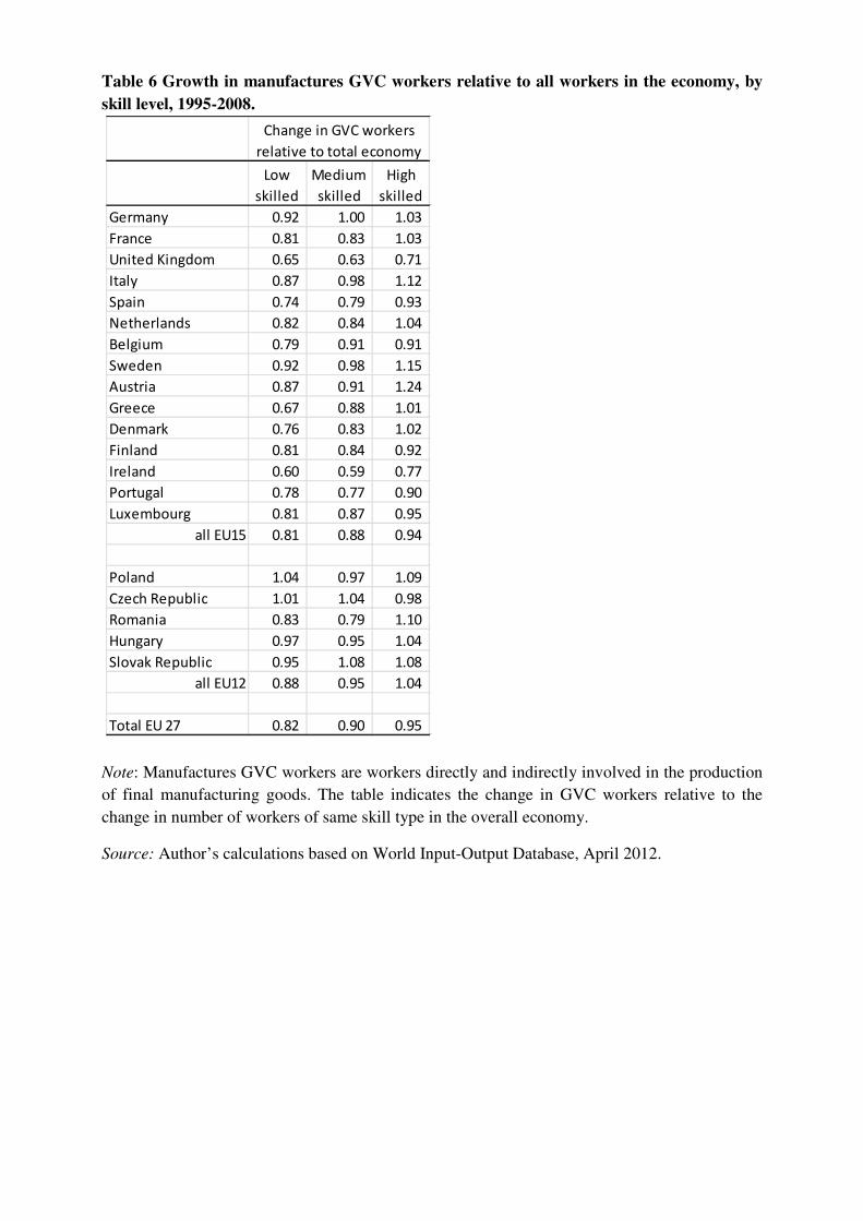
Table 6 Growth in manufactures GVC workers relative to all workers in the economy, by
skill level, 1995-2008.
Note: Manufactures GVC workers are workers directly and indirectly involved in the production
of final manufacturing goods. The table indicates the change in GVC workers relative to the
change in number of workers of same skill type in the overall economy.
Source: Author’s calculations based on World Input-Output Database, April 2012.
Low
skilled
Medium
skilled
High
skilled
Germany 0.92 1.00 1.03
France 0.81 0.83 1.03
United Kingdom 0.65 0.63 0.71
Italy 0.87 0.98 1.12
Spain 0.74 0.79 0.93
Netherlands 0.82 0.84 1.04
Belgium 0.79 0.91 0.91
Sweden 0.92 0.98 1.15
Austria 0.87 0.91 1.24
Greece 0.67 0.88 1.01
Denmark 0.76 0.83 1.02
Finland 0.81 0.84 0.92
Ireland 0.60 0.59 0.77
Portugal 0.78 0.77 0.90
Luxembourg 0.81 0.87 0.95
all EU15 0.81 0.88 0.94
Poland 1.04 0.97 1.09
Czech Republic 1.01 1.04 0.98
Romania 0.83 0.79 1.10
Hungary 0.97 0.95 1.04
Slovak Republic 0.95 1.08 1.08
all EU12 0.88 0.95 1.04
Total EU 27 0.82 0.90 0.95
Change in GVC workers
relative to total economy
Fragmentation, Incomes and Jobs.
An analysis of European competitiveness
Appendix
Tables and figures for full set of 40 countries

Appendix Table 1 Real GVC income in EU27 countries, all manufactures
Note: Real GVC income for all manufactures and in constant 1995 prices using US CPI as deflator. Decomposed
into part due to domestic demand and part due to foreign demand. Source: Author’s calculations based on World
Input-Output Database, April 2012
1995 2008 1995 2008
United States 1,311,507 1,376,188 25.9 33.0
Japan 1,153,965 677,803 24.6 41.8
China 277,033 1,116,642 35.3 48.7
Germany 617,836 665,164 46.3 69.9
France 292,330 330,216 53.1 60.0
United Kingdom 253,548 260,443 52.6 68.5
Italy 289,055 354,158 45.2 52.8
Spain 127,696 171,836 39.1 53.3
Russian Federation 80,174 246,830 42.6 47.3
Brazil 163,652 265,070 15.7 26.0
Canada 123,880 190,037 65.8 65.8
India 113,531 229,321 17.7 29.3
Mexico 98,526 208,217 32.9 36.5
Australia 67,599 112,593 43.9 55.3
South Korea 141,553 157,002 45.2 67.8
Netherlands 94,133 118,973 79.3 87.8
Turkey 73,333 122,295 22.5 35.3
Indonesia 83,421 113,625 28.5 38.7
Poland 33,439 85,700 42.7 63.0
Belgium 66,357 69,783 84.1 89.2
Sweden 55,536 70,548 70.3 77.5
Taiwan 82,727 73,053 60.9 79.4
Austria 50,081 62,674 53.9 78.5
Greece 20,468 30,564 17.5 31.3
Denmark 36,484 41,700 79.8 87.5
Finland 28,868 36,952 64.5 74.3
Ireland 21,583 40,480 88.3 88.1
Portugal 23,730 27,228 48.5 59.6
Czech Republic 14,477 41,450 57.3 79.0
Romania 11,896 32,585 32.4 44.4
Hungary 11,120 27,140 44.9 73.1
Slovak Republic 5,060 17,624 64.4 79.8
Luxembourg 3,784 6,743 94.1 97.5
Slovenia 5,150 8,548 69.0 86.3
Lithuania 1,522 6,637 54.0 64.0
Bulgaria 3,900 7,134 44.7 65.0
Latvia 1,028 3,108 57.4 69.1
Cyprus 1,304 1,547 43.7 52.2
Estonia 936 3,041 68.7 82.0
Malta 854 1,003 50.4 78.5
Real GVC income (in
mil constant $)
Real GVC income
due to foreign
demand (%)

Appendix Table 2 Decomposition of change in manufactures GVC income due to change in
production structure and final demand
Note: Change in real GVC income from Table 1. The change is decomposed by keeping the production structures
constant while final demand changes, and by keeping the final demand constant, while production structures change.
This additive decomposition can be done keeping 1995 or 2008 levels constant, and average weights are used.
Source: Author’s calculations based on World Input-Output Database, April 2012.
Total
change
(mil US$)
keeping
production
structures
constant
keeping
final
demand
constant
United States 64,681 171,915 -107,234
Japan -476,162 -320,264 -155,898
China 839,609 738,239 101,370
Germany 47,328 111,625 -64,297
France 37,886 79,199 -41,313
United Kingdom 6,895 8,637 -1,742
Italy 65,104 83,767 -18,664
Spain 44,140 49,120 -4,980
Russian Federation 166,656 127,872 38,784
Brazil 101,418 102,843 -1,425
Canada 66,157 48,487 17,670
India 115,790 116,648 -858
Mexico 109,690 97,749 11,941
Australia 44,993 28,409 16,584
South Korea 15,449 31,724 -16,275
Netherlands 24,840 26,925 -2,086
Turkey 48,963 50,299 -1,336
Indonesia 30,204 20,167 10,037
Poland 52,261 47,986 4,275
Belgium 3,426 12,606 -9,180
Sweden 15,012 18,434 -3,422
Taiwan -9,675 -2,414 -7,260
Austria 12,593 15,799 -3,206
Greece 10,095 10,977 -882
Denmark 5,217 6,910 -1,694
Finland 8,085 9,549 -1,465
Ireland 18,897 16,383 2,514
Portugal 3,498 3,620 -121
Czech Republic 26,973 23,229 3,743
Romania 20,689 18,584 2,105
Hungary 16,020 14,371 1,649
Slovak Republic 12,564 11,338 1,226
Luxembourg 2,959 1,600 1,359
Slovenia 3,398 2,694 704
Lithuania 5,115 3,930 1,185
Bulgaria 3,235 2,997 238
Latvia 2,080 1,590 490
Cyprus 243 84 159
Estonia 2,106 1,321 785
Malta 148 5 144
Change in real GVC income between 1995
and 2008

Appendix Table 3 Revealed comparative advantage, major EU countries, 1995 and 2008.
(see next page)
1995 2008 1995 2008 1995 2008 1995 2008 1995 2008 1995 2008
United States 1.00 1.17 1.12 1.07 0.88 0.97 0.83 0.80 0.81 0.62 1.27 1.10
Japan 0.58 0.54 1.51 1.33 0.88 0.88 1.48 1.55 0.65 0.39 1.09 1.42
China 0.87 0.36 0.97 1.75 1.03 0.83 0.99 1.07 1.77 1.65 0.55 0.86
Germany 1.10 0.80 0.87 0.95 0.72 0.67 1.37 1.43 0.76 0.65 1.26 1.54
France 1.08 1.08 0.80 0.72 0.99 1.04 0.86 0.93 0.85 0.77 1.38 1.30
United Kingdom 1.30 1.30 0.98 0.81 0.83 0.78 0.99 0.95 0.96 0.90 0.95 1.07
Italy 0.92 0.70 0.65 0.65 0.72 0.75 1.32 1.59 1.95 1.82 0.67 0.76
Spain 0.96 0.89 0.52 0.54 1.17 1.17 0.58 0.85 1.43 1.07 1.16 1.24
Russian Federation 1.73 2.00 0.48 0.50 1.27 1.11 1.00 1.06 0.72 0.59 0.79 0.65
Brazil 1.20 1.00 0.78 0.62 1.16 1.16 0.69 0.99 1.47 1.13 0.79 1.03
Canada 0.99 1.37 0.66 0.56 0.98 0.98 0.72 0.78 0.74 0.73 1.64 1.33
India 0.93 0.87 0.41 0.77 1.06 1.11 0.80 0.99 2.08 1.87 0.78 0.62
Mexico 1.91 1.70 0.59 0.57 1.35 1.36 0.50 0.51 0.64 0.56 0.98 1.02
Australia 1.03 0.93 0.52 0.79 1.50 1.18 0.73 1.14 1.08 0.82 0.70 0.86
South Korea 0.54 0.34 1.33 1.83 0.79 0.53 0.93 1.12 1.29 0.81 1.37 1.80
Netherlands 1.23 1.40 0.75 0.70 1.31 1.13 0.86 0.96 0.85 0.81 0.68 0.74
Turkey 1.21 0.63 0.40 0.42 1.12 1.32 0.89 0.76 1.95 2.53 0.57 0.50
Indonesia 0.87 0.96 0.63 0.70 1.53 1.53 0.32 0.42 1.53 1.28 0.86 0.93
Poland 0.92 0.84 0.51 0.60 1.42 1.25 0.73 0.92 1.33 1.09 0.72 1.03
Transport
equipmentChemicals
Electrical
machinery Food products
Non-elec.
machinery and
metal Non-durables

Appendix Table 3 Revealed comparative advantage, major EU countries, 1995 and 2008. (continued)
Note: Revealed comparative advantage calculated as country share in world GVC income for a group of manufactures divided by
same ratio for all manufactures. Food manufacturing products (Food: produced in ISIC rev.3 industries 15 & 16), Other non-durable
products (Tex: 17 to 20, 36, 37); Chemical products (Chem: 23 to 26), Machinery & metal products (Mach: 27 to 29); Electrical
machinery products (Elec: 30 to 33) and Transport equipment (Tra: 34, 35).
Source: Author’s calculations based on World Input-Output Database, April 2012.
1995 2008 1995 2008 1995 2008 1995 2008 1995 2008 1995 2008
Belgium 1.30 1.30 0.67 0.69 0.96 0.95 0.95 1.04 0.99 0.87 1.16 1.05
Sweden 0.88 0.85 1.18 1.16 0.76 0.65 1.19 1.49 0.61 0.61 1.29 1.26
Taiwan 0.78 0.50 1.43 2.59 0.76 0.52 1.27 1.29 1.40 0.94 0.77 0.80
Austria 1.03 0.74 0.90 0.97 0.91 0.76 1.24 1.61 1.22 0.94 0.68 1.01
Greece 0.87 0.99 0.31 0.41 1.82 1.62 0.21 0.63 1.82 1.47 0.30 0.40
Denmark 0.99 1.42 0.70 0.90 1.43 1.09 1.03 1.20 1.02 0.75 0.47 0.52
Finland 0.74 0.70 1.26 1.56 0.97 0.77 1.22 1.50 0.75 0.63 0.62 0.75
Ireland 1.27 1.69 1.21 1.37 1.47 1.05 0.44 0.45 0.46 0.47 0.33 0.45
Portugal 0.81 0.76 0.50 0.64 1.04 1.06 0.53 0.72 2.69 2.22 0.54 0.71
Czech Republic 0.88 0.61 0.60 0.97 1.13 0.81 1.27 1.25 1.16 0.90 0.84 1.51
Romania 0.87 0.76 0.49 0.45 1.55 1.35 0.75 0.76 1.55 1.48 0.54 1.06
Hungary 1.20 1.10 0.62 1.28 1.47 0.94 0.64 0.90 1.09 0.60 0.68 1.18
Slovak Republic 1.23 0.60 0.62 1.18 1.09 0.66 0.88 1.24 1.26 0.92 0.79 1.39
Luxembourg 1.18 0.87 0.72 0.88 0.86 0.83 1.21 1.28 1.05 1.23 1.01 1.01
Slovenia 1.16 1.17 0.80 0.87 0.72 0.59 1.06 1.45 1.78 1.14 0.75 0.99
Lithuania 1.17 1.30 0.37 0.42 1.66 1.42 0.68 0.68 1.50 1.34 0.32 0.57
Bulgaria 0.97 0.78 0.28 0.50 1.73 1.32 0.58 1.16 1.46 1.76 0.42 0.47
Latvia 0.61 0.61 0.41 0.52 1.58 1.56 0.54 0.73 1.61 1.28 0.41 0.67
Cyprus 0.87 0.90 0.23 0.44 1.60 1.65 0.41 0.69 2.03 0.95 0.20 0.43
Estonia 0.74 0.73 0.49 0.85 1.59 1.12 0.50 0.93 1.87 1.56 0.28 0.63
Malta 1.13 1.20 0.95 1.28 0.75 0.75 0.62 0.64 2.17 1.42 0.68 0.96
Chemicals
Electrical
machinery Food products
Non-elec.
machinery and
metal Non-durables
Transport
equipment

9
Appendix Table 5 Manufactures GVC workers, 1995 and 2008
Note: GVC workers are workers directly and indirectly involved in the production of manufacturing goods. First
four columns indicate the change in the number of GVC workers by sector between 1995 and 2008. Next four
columns indicate the total number of GVC workers by sector in 2008. Last column is the total number of workers in
the economy. Source: Author’s calculations based on World Input-Output Database, April 2012.
Agricul
ture
Manufa
cturing Services
All
sectors
Agricul
ture
Manufa
cturing Services
All
sectors
1995 2008
United States 16.0 11.1 1,143 8,837 6,892 16,872 -331 -3,144 -1,138 -4,612
Japan 22.6 19.4 1,298 6,491 4,417 12,207 -794 -2,225 148 -2,871
China 31.7 33.3 121,342 87,568 49,468 258,378 9,963 20,508 11,965 42,436
Germany 26.8 26.4 400 5,481 4,766 10,647 -161 -666 1,388 561
France 22.0 18.7 303 2,195 2,355 4,853 -96 -423 368 -151
United Kingdom 20.1 12.6 115 1,946 1,931 3,992 -128 -1,148 -347 -1,624
Italy 29.1 25.5 333 3,553 2,559 6,444 -192 -234 517 91
Spain 23.2 17.5 271 1,827 1,494 3,592 -97 185 353 440
Russian Federation 24.7 21.9 4,259 6,749 6,228 17,237 -1,403 -2,120 2,198 -1,325
Brazil 29.6 28.7 8,347 9,490 9,823 27,660 -705 2,450 4,118 5,863
Canada 20.8 16.0 157 1,138 1,482 2,777 -102 -136 193 -45
India 27.9 27.3 57,926 41,933 26,483 126,343 2,118 10,896 7,025 20,039
Mexico 30.3 24.4 2,817 6,128 3,205 12,150 -400 1,403 1,121 2,124
Australia 18.2 14.5 165 641 855 1,661 -48 3 196 150
South Korea 29.7 22.8 655 2,646 2,077 5,378 -468 -735 524 -679
Netherlands 22.8 19.0 89 643 929 1,661 -42 -87 158 29
Turkey 27.1 30.4 1,778 3,115 1,554 6,446 -341 620 584 863
Indonesia 32.1 25.6 13,921 7,427 5,725 27,073 -1,899 -425 1,380 -944
Poland 31.0 28.8 917 2,278 1,347 4,542 -468 81 368 -19
Belgium 25.0 20.9 31 399 503 933 -18 -86 72 -32
Sweden 22.7 21.0 36 481 443 959 -23 -49 94 22
Taiwan 30.9 29.2 113 1,900 1,028 3,041 -204 159 187 142
Austria 24.8 22.6 104 463 393 960 -46 -35 120 40
Greece 21.0 15.0 97 374 247 717 -202 17 34 -151
Denmark 23.9 19.6 41 271 257 569 -25 -66 51 -41
Finland 23.6 19.7 39 248 211 498 -25 -12 51 14
Ireland 31.5 18.8 59 168 168 394 -35 -17 40 -11
Portugal 28.9 21.7 191 602 343 1,136 -57 -139 20 -176
Czech Republic 30.8 30.9 93 990 553 1,636 -59 74 35 50
Romania 34.0 27.6 684 1,388 517 2,588 -356 -222 -68 -646
Hungary 31.6 29.3 129 675 400 1,204 -145 13 63 -69
Slovak Republic 28.2 29.6 22 392 249 663 -35 19 85 69
Luxembourg 20.3 17.4 1 23 36 61 -1 1 16 17
Slovenia 34.0 26.9 20 163 83 266 -10 -47 11 -46
Lithuania 26.8 21.3 32 183 109 324 -61 -27 14 -73
Bulgaria 30.7 28.6 276 544 276 1,096 32 -73 58 17
Latvia 23.4 16.9 20 102 69 191 -20 -32 16 -36
Cyprus 18.5 11.5 3 24 19 46 -2 -12 4 -9
Estonia 31.7 22.4 10 88 49 147 -26 -20 -8 -53
Malta 24.0 17.9 1 17 12 29 0 -6 2 -4
Change in manufactures GVC
workers between 1995 and 2008
(in thousands) employed in
Manufactures GVC workers in
2008 (in thousands) employed in
Manufactures
GVC workers as
(%) share of all
workers in the
economy

10
Appendix Table 6 Change in Manufactures GVC workers, by skill level, 1995-2008.
Note: GVC workers are workers directly and indirectly involved in the production of manufacturing goods. First
four columns indicate the change in the number of GVC workers by skill type. Last four columns indicate the
change in GVC workers relative to the change in number of workers of same skill type in the overall economy.
Source: Author’s calculations based on World Input-Output Database, April 2012.
Low
skilled
Medium
skilled
High
skilled
United States 0.66 0.71 0.69
Japan 0.92 0.90 0.87
China 1.12 0.99 1.00
Germany 0.92 1.00 1.03
France 0.81 0.83 1.03
United Kingdom 0.65 0.63 0.71
Italy 0.87 0.98 1.12
Spain 0.74 0.79 0.93
Russian Federation 0.90 0.90 0.98
Brazil 0.99 1.18 1.00
Canada 0.74 0.77 0.91
India 0.97 0.99 1.00
Mexico 0.82 0.78 0.96
Australia 0.81 0.82 0.90
South Korea 0.68 0.85 0.86
Netherlands 0.82 0.84 1.04
Turkey 1.21 1.14 1.03
Indonesia 0.81 0.96 0.94
Poland 1.04 0.97 1.09
Belgium 0.79 0.91 0.91
Sweden 0.92 0.98 1.15
Taiwan 0.99 1.03 1.00
Austria 0.87 0.91 1.24
Greece 0.67 0.88 1.01
Denmark 0.76 0.83 1.02
Finland 0.81 0.84 0.92
Ireland 0.60 0.59 0.77
Portugal 0.78 0.77 0.90
Czech Republic 1.01 1.04 0.98
Romania 0.83 0.79 1.10
Hungary 0.97 0.95 1.04
Slovak Republic 0.95 1.08 1.08
Luxembourg 0.81 0.87 0.95
Slovenia 0.85 0.82 0.85
Lithuania 0.75 0.80 0.93
Bulgaria 0.94 0.98 1.53
Latvia 0.69 0.71 0.88
Cyprus 0.60 0.68 0.65
Estonia 0.65 0.68 0.81
Malta 0.74 0.86 1.23
Change in GVC workers
relative to total economy

11
Figure 2 Share of foreign value added in production of final manufacturing products.
Note: This graph shows the foreign value added share in the output value of final manufacturing
products produced in a country. The remaining share is value added by the domestic economy.
Share in 1995 and change during 1995-2008 period. A higher share indicates more international
fragmentation of production.
Source: Author’s calculations based on World Input-Output Database, April 2012.
0.0 0.1 0.2 0.3 0.4 0.5
Russian Federation
Brazil
India
Australia
Turkey
Indonesia
Poland
Netherlands
Spain
Italy
United Kingdom
France
Germany
South Korea
Taiwan
Japan
China
Mexico
Canada
United States
1995 2008 over 1995

Top Related