


Languages
Pages
Legal

GEOMECHANICAL CHARACTERIZATION AND RESERVOIR SIMULATION OF A CO2
SEQUESTRATION PROJECT IN A MATURE OIL FIELD, TEAPOT DOME, WY
A DISSERTATION
SUBMITTED TO THE DEPARTMENT OF GEOPHYSICS AND THE COMMITTEE ON GRADUATE STUDIES
OF STANFORD UNIVERSITY IN PARTIAL FULFILLMENT OF THE REQUIREMENTS
FOR THE DEGRREE OF DOCTOR OF PHILOSOPHY
Laura Chiaramonte
December 2008

ii
© Copyright by Laura Chiaramonte 2008
All rights Reserved

iii
I certify that I have read this dissertation and that in my opinion it is fully adequate, in scope and quality, as a dissertation for the degree of Doctor of Philosophy.
_______________________________ (Mark D. Zoback) Principal Adviser
I certify that I have read this dissertation and that in my opinion it is fully adequate, in scope and quality, as a dissertation for the degree of Doctor of Philosophy.
_______________________________ (S. Julio Friedmann)
I certify that I have read this dissertation and that in my opinion it is fully adequate, in scope and quality, as a dissertation for the degree of Doctor of Philosophy.
_______________________________ (Jerry M. Harris)
Approved for the University Committee on Graduate Studies.
iv
ABSTRACT There is increasing evidence that reinforces the view that climate and greenhouse
gas cycles are intimately related. Carbon dioxide (CO2) is the main anthropogenic gas
contributing to the greenhouse effect and global warming. The main anthropogenic
source of CO2 comes from the burning of fossil fuels which currently dominates
commercially supplied energy worldwide. Since it is generally accepted that
concentration in the atmosphere of greenhouse gases, in particular CO2, must be
restricted, a technique capable of reducing the CO2 emissions to the atmosphere
while still allowing the use of fossil fuels is a key advance in the short to medium
term solution to this problem. One such solution that has been proposed is Carbon
Capture and Sequestration (CCS) has been.
However, for CCS to be a viable carbon management solution, one of the main
issues to be addressed is the risk of CO2 leakage. In light of this, a key step in the
evaluation of any potential site being considered for geologic carbon sequestration is
the ability to predict whether the increased pressures associated with CO2
sequestration are likely to affect seal capacity.
In this dissertation, I present my contribution towards the understanding and
prediction of the risk of CO2 leakage through natural pathways (i.e. faults and
v
fractures). The main portion of this dissertation deals with geomechanical aspects of
CO2 Sequestration in Teapot Dome, WY, a mature oil field. The last study investigates
the use of induce microseismicity to enhance permeability and injectivity in tight
reservoirs and to monitor carbon sequestration projects.
In the first three projects, the Tensleep Formation, a Pennsylvanian age eolian
fractured sandstone, is evaluated as the target horizon for a pilot CO2 EOR‐carbon
storage experiment, in a three‐way closure trap against a bounding fault, termed the
S1 fault. In the first study, a geomechanical model of the Tensleep Fm. has been
developed to evaluate the potential for CO2 injection inducing slip on the S1 fault and
thus threatening seal integrity. The geomechanical analysis demonstrated that CO2
sequestration will not induce slip on the reservoir‐bounding fault, nor is fracking the
cap rock a concern. However, various sets of pre‐existing minor faults in the reservoir
are critically stressed (i.e., active) in the current stress field. Hence, raising pore
pressure during sequestration will activate slip on these minor faults. The presence of
these minor faults enhances formation permeability and injectivity of CO2. However,
the potential for slip on these features could potentially compromise the top seal
capacity of the Tensleep if these minor faults extend up into the cap rock.
In the second study, a 3D reservoir model and fluid flow simulation of the
Tensleep Fm., under these geomechanical constraints, was developed to model the
migration of the injected CO2 as well as to obtain limits on the rates and volumes of
CO2 that can be injected without compromising seal integrity. The results of the
numerical simulations corroborate the analytical results of the geomechanical
analysis that seal integrity will not be compromised by the pilot injection. The
simulations also showed that the EOR pilot project could recover from 8% to 30%
incremental oil, by sequestering 2175 tonnes (42 MMcf) in 6 weeks or 4350 tonnes
(168 MMcf) in 12 weeks respectively. However mobility of CO2 through the highly
permeably fracture network could present a problem and a well control strategy
needs to be implemented to co‐optimize EOR and sequestration.
vi
In the third study, we test an Amplitude Versus Angle and Azimuth (AVAZ)
analysis to identify the presence of fractures using wide‐azimuth 3D seismic data. The
objective of the project was to obtain a 3D characterization of the fracture network
on both the reservoir and the caprock that will allow for a more accurate assessment
of the impact of these features in reservoir permeability and in the risk of CO2
leakage. The AVAZ results were calibrated with fracture intensity and orientations
obtained from FMI logs recorded in the area as well as stress orientation and the
macro fault network of the anticline. During the analysis of these results, we did not
find enough evidence to indicate whether the observed anisotropy is influenced by
stress, structural or sedimentary features. Furthermore, it is possible that the
method does not work with this data set, because particularities of this setting do
not follow the assumptions of the method.
In the final project of this dissertation, we focus on deep saline formations, which
have great potential for geologic sequestration of CO2. Such formations are
widespread, and in theory, easily accessed from point sources of CO2, such as power
plants, factories, etc. Unfortunately, many deep saline aquifers of the mid‐
continental U.S. appear to have very low porosity and permeability, which results in
limited injectivity and storage capacities.
In this study, we investigate the use of induced microseismicity to enhance
permeability and injectivity of a tight formation as well as to monitor a carbon
sequestration project. During the injection‐induced microseismicity stimulation,
more than 10,000 metric tons of supercritical CO2 were injected into the Bass Island
Dolomite (BILD) during a period of 40 days. A total of 803 events were recorded in
more of three sensors in each of the two monitoring arrays. However, no definite
seismic activity could be related to the injection in the BILD. A preliminary possible
hypothesis relates this microseismicity to a CO2 injection from a deeper and
preexisting EOR project in this area, which could be migrating upwards along the
monitoring wells.

vii
ACKNOWLEDGMENTS
The list of people I would like to thank for their help and support during my PhD
study is quite long. But especially, I would like to thank my advisor Mark Zoback who
has been a wonderful mentor, that not only taught me about geomechanics but also
serve as a great role model both as a scientist and as a person. He has an enthusiasm
for geophysics and for life in general that is very motivating. He also makes sure to
create a supportive, friendly, challenging, and collaborative work environment. He
pays particular attention in encouraging work‐life balance for his students. Thank you
Mark!
I would also like to thank my committee members, Julio Friedmann, Jerry Harris,
and Lynn Orr for their support, help, and patience. Their insight and suggestions have
greatly improved my work and my knowledge over these past few years. Additionally
I would like to thank the help and guidance of the members of my original Qualifying
Exam committee Gary Mavko and Steve Graham. Steve also kindly chair my defense
and has been and invaluable source of knowledge, support, and friendship during all
my years at Stanford.
I would like to thank the people that, at different stages these past years, have
helped me with my research. Paul Hagin, thanks for your support, insight and helpful
discussions. Also many thanks to Tapan Mukerji, Tony Kovscek, Khalid Aziz, Kyle
Spikes, Andres Mantilla, Fernando Garcia Parodi, Alejo Lopez, and Joe Morris.

viii
I would like to acknowledge the Global Climate and Energy Project for their
funding as well as to the Fulbright Scholarship, which sponsored me to get to
Stanford in the first place.
I want to acknowledge my collaborators on the several projects I have worked. I
greatly enjoyed working with them and also benefit enormously from their
contributions. I especially would like to thank Julio Friedmann and Vicki Stamp. Julio
has been an excellent guide to the world of carbon sequestration and his suggestions
greatly improved this dissertation. Vicki has been a wonderful collaborator, always
available for my endless questions, and always with the sweetest disposition. I also
want to thank the valuable help of RMOTC staff which was always very helpful for my
requests of data: Tom Anderson, Brian Black (sorry for the many requests!), and
Mark Milliken. Similarly, I would like to thank Neeraj Gupta and Jackie Gerst of the
Battelle Memorial Institute. And finally, I enjoyed working and learning from Marco
Bohnhoff and David Gray from CGGVeritas.
I would like to thank all the past and present members of the Stress and Crustal
Mechanics research group: Marco Bohnhoff, Naomi Boness, Lourdes Colmenares,
Alvin Chan, Indrajit Das, Amy Day‐Lewis, Paul Hagin, Robert Heller, Owen Hurd,
Madhur Johri, Amie Lucier, Ellen Mallman, Pijush Paul, Hannah Ross, Norm Sleep,
Hiroke Sone, George Thompson, John Vermylen, Charley Weiland, Sonata Wu. And
many, many thanks to Susan Phillips Moskowitz for taking such a good care of all of
us.
One of the greatest things about studying at Stanford is the richness of the
people here. I greatly benefitted from studying, working, and sharing time with other
students, but even more important, I found many great friends! And the same
applies to the life outside Stanford, by playing soccer with friends, sharing many
asados, and playing even more soccer… ok, I did other things besides playing soccer,
but definitely I spent many of my most memorable moments in the fields (Roble,
Sand Hill Road, …). It kept me sane in stressful moments and I even met my Búlgaro
there!!! I would like to thank all the friends with whom we shared many

ix
unforgettable moments: Fabrizio, Kyle, Ezequiel, Tricia, Nico, Jeff, María Leticia, Karla,
Paula, Valeria, Mariel, Jordan, Kevin. Thank you all!
I would also like to thank two people that had have the most influence in my
career since the beginning and help me get here: my undergraduate advisor from
Universidad de Buenos Aires, Victor A. Ramos and Rene Manceda. Thank you!
I also wouldn’t be here if it weren’t for the love, support and encouragement
from my family: my dad José Carlos, my mom Susana, my sister Marina, my brother
Gustavo, and their kids: Mariano, Federico, Julieta, Clarita, and Luciana, who make
me laugh and love.
Finally, I want to thank my husband Tzanko for his love, support, patience, the
shared fun, and amazing life he makes me live!

x
TABLE OF CONTENTS
ABSTRACT ….………………………………………………………...…………………………… IV
ACKNOWLEDGMENTS ………………………………………………………..…….…………... VII
TABLE OF CONTENTS …………………………………………………………………………….… X
LIST OF TABLES ………………………………………………………………..……………….. XV
LIST OF FIGURES ……………………………………………………………………….……… XVII
CHAPTER 1 – INTRODUCTION …..……………………………………………..…….………… 1
1.1 OVERVIEW AND MOTIVATION .......…………………………………………….…..…………….. 1
1.2 THESIS OUTLINE ………………………………………………………..…………………………….… 3
CHAPTER 2 ‐ TEAPOT DOME OIL FIELD – NATIONAL GEOLOGICAL CARBON STORAGE TEST CENTER……………………………………………..………………………….………………. 6
2.1 ABSTRACT ….………………………………………………………………………………………….... 6
2.2 INTRODUCTION ……………………………………………..………………………………………..... 7
2.2.1 Greenhouse effect, climate change and CO2 emissions …………..………….….……… 7
2.2.2 Previous CO2 Sequestration around the world …………………………………………..… 10
2.2.3 CO2 Sequestration Underground – Storage Options ……………………………..…..…. 11
2.2.4 CO2 Sequestration in mature Oil & Gas fields …………………………………………….… 12
2.2.5 Risk of Leakage during CO2 Sequestration …………………………………..……….…….… 12
2.3 TEAPOT DOME …………………………………………………………………………...……………. 13
xi
2.3.1 History of Teapot Dome ………………………………..…………………………....………………. 14
2.3.2 Regional Geology ………………………………..……………………………………...…..………….. 15
2.3.3 Teapot Dome Anticline ………………………………..………..……………………….………..…. 16
2.3.4 Sequestration and Leakage Projects …………………..……………………………………… 19
2.3.4.1 S1 fault area ‐ Section 10 …………………………….………..………………….. 19
2.3.4.2 S2 fault area ……………………………………………………………….…………….. 20
2.3.5 Stratigraphy ………………………………..……………………………………………..………….….. 21
2.3.5.1 Tensleep Formation ………………………………...……………………………….. 24
2.3.5.2 Seal ………………………………..…………………….………………….……………….. 28
2.3.6 Fractures ………………………………………………………………………………………….………… 28
2.4 TEAPOT DOME CARBON STORAGE TEST CENTER …………………..……………………….… 29
2.4.1 Data Set ………………………………….………………………………………………….………………. 30
2.4.1.1 Seismic ……………….……………………………………………….……..………………. 31
2.4.1.2 Well logs ……………………………………….……………………..…………………… 31
2.4.2 Pilot project ……………….…………………………………………………………………………….… 33
2.4.3 CO2 Source ………………..…………….…………………………………………………..……………… 33
2.5 SUMMARY ….……………………………………………………..…………………………………… 35
CHAPTER 3 ‐ SEAL INTEGRITY AND FEASIBILITY OF CO2 SEQUESTRATION IN THE TEAPOT
DOME EOR PILOT: GEOMECHANICAL SITE CHARACTERIZATION .......................... 36
3.1 ABSTRACT …………………………………………………………………………...………………… 36
3.2 INTRODUCTION …………………………………………………………………….…….…………… 37
3.3 TEAPOT DOME CO2‐EOR CARBON STORAGE PILOT ………………………..………………. 38
3.4 GEOLOGY OF TEAPOT DOME ………………………………………………………………………… 39
3.5 GEOMECHANICAL CHARACTERIZATION ……………………………………………………………. 42
3.6 FAULT SLIP POTENTIAL USING COULOMB CRITERION …………………………………………. 48
3.7 CRITICAL PRESSURE PERTURBATION SENSITIVITY ANALYSIS …………….……………..…... 51
3.8 HYDRAULIC FRACTURE LIMIT FOR CAPROCK ………………………………….………………… 54
3.9 FRACTURES AT TEAPOT DOME …………………………………………………….……….…….. 55
3.10 S2 FAULT ZONE STABILITY ANALYSIS FOR A POTENTIAL LEAKAGE EXPERIMENT ….……. 59
3.11 SUMMARY …..……………………………………………………………………..……………….. 61

xii
CHAPTER 4 ‐ 3D STOCHASTIC RESERVOIR MODEL AND FLUID FLOW SIMULATION OF THE
TENLSEEP FORMATION ……………………………………..……………………..………….. 63
4.1 ABSTRACT …………………………………………………...………………………………..………. 63
4.2 INTRODUCTION ………………………………………….……………………………………………. 64
4.3 3D STOCHASTIC RESERVOIR MODEL …………………...……………………………………….. 65
4.3.1 RESERVOIR CHARACTERIZATION IN SECTION 10 (S1 FAULT AREA) ………….....……………….. 67
4.3.2 USING GEOSTATISTIC TO POPUALATE THE 3D MODEL WITH POROSITY AND PERMEABILITY DISTRIBUTIONS …………..………………………………..………………………….………………… 70
4.4 MODELING CO2‐EOR PROCESSES IN A FRACTURED RESERVOIR …………….……………. 75
4.4.1 PREVIOUS CO2‐EOR PROJECTS ………………………………………………………………………….. 76
4.4.2 PREVIOUS FLUID FLOW SIMULATIONS AT TEAPOT DOME ……………….………..………………. 77
4.4.3 CO2 PROCESS MECHANISMS ……………………………………………………….……...…………….. 77
4.4.4 OPTIONS FOR CO2 FLOOD DESIGN ………………………………………………………………….….. 78
4.5 FLUID FLOW SIMULATION ……………………………………….………………………………….. 80
4.5.1 RESERVOIR DATA …………………………………………………….………………………………………. 80
4.5.2 SIMULATION SET UP ………………………………………………….………………….…………………. 82
4.5.2.1 MODEL ……………………………………………………..…………………………………. 82
4.5.2.2 MATRIX POROSITY AND PERMEABILITY ………………..………………………………. 82
4.5.2.3 FRACTURE POROSITY AND PERMEABILITY ……………….……………….……………. 83
4.5.2.4 FRACTURE SPACING ……………………………………………..…………………………. 83
4.5.2.5 MATRIX RELATIVE PERMEABILITY …………………………………………….………… 83
4.5.2.6 FRACTURE RELATIVE PERMEABILITY …………………………………………....……… 86
4.5.2.7 CO2 RELATIVE PERMEABILITY …………………………………………………………..… 86
4.5.2.8 CAPILLARY PRESSURE ……………………………………………………………….……… 87
4.5.2.9 WETTABILITY …………………………………………………………………………………… 88
4.5.2.10 EQUATION OF STATE ………………………………………………………..…………… 88
4.5.2.11 AQUIFER ………………………………………………………………………….……….… 90
4.5.3 INITIAL CONDITIONS ………………………………………………………………………………………… 90
4.5.4 HISTORY MATCHING …………………………………………………………………………...…………… 91
4.5.4.1 SENSITIVITY ANALYSIS TO HM PARAMETERS ……………………………………….… 91
4.5.5 BASE CASE SCENARIO ……………………………………………………………………………..………… 99
4.5.6 PILOT CO2‐EOR SIMULATIONS ………………………………………………………………………… 102
xiii
4.5.7 SEQUESTRATION POTENTIAL ……………………………………………….………….………………… 108
4.5.7.1 TESTING STORAGE CAPACITY OF RESERVOIR ……………………….………………… 109
4.5.8 SENSITIVITY ANALYSIS OF PILOT CO2 ‐EOR …………..……………………….….………………… 111
4.5.8.1 FRACTURE PERMEABILITY (KF) …….…………………………………………………… 111
4.5.8.2 FRACTURE POROSITY (øF) …..…….…………………………………………………… 112
4.5.8.3 FRACTURE SPACING (SPF) ……………………….……………………………………… 112
4.5.8.4 RELATIVE PERMEABILITY CURVES (KREL) ….………………..………………………… 113
4.5.8.5 MATRIX POROSITY & PERMEABILITY …………………….…………………………… 115
4.5.8.5 GRID SIZE …….………………….…………………………….…………………………… 115
4.5.9 SENSITIVITY ANALYSIS OF PILOT CO2‐EOR WITHOUT GAS CONSTRAINTS …..……..………… 116
4.5.8.1 FRACTURE PERMEABILITY ………………………………………………..……………… 111
4.6 SUMMARY …………………………………………………………………………….……….……… 121
CHAPTER 5 ‐ FRACTURE DETECTION USING AMPLITUDE VERSUS ANGLE
AND AZIMUTH AT TEAPOT DOME OIL FIELD, WY ………………..………….. 124
5.1 ABSTRACT………………….………………….……………………………………………..………… 124
5.2 INTRODUCTION – MOTIVATION……………………………….………………………….………. 125
5.3 SEISMIC ANISOTROPY ………………….……………………………………………………………. 126
5.4 AVAZ METHOD IN FRACTURED RESERVOIRS ………….……………………….………………. 128
5.5 APPLICATION TO TEAPOT DOME – RESULTS ANALYSIS ……….………………………….…. 131
5.5.1 TENSLEEP ANISOTROPY………………………………………………………………………….…………. 139
5.5.1.1 SECTION 10 – S1 FAULT AREA……………………………………………...…………… 139
5.5.1.2 S2 FAULT AREA ……………………………………………………………………………… 144
5.5.1.3 S3‐S4 FAULT AREA ……………………………………………………….………………… 145
5.5.2 TENSLEEPB ANISOTROPY …………………………………………………………………………………… 147
5.5.3 OPECHE ANISOTROPY ……………………………………………………………………………………… 152
5.5.4 DUNE MORPHOLOGY AND ACQUISITION PATTERN ………………………..……………………….. 158
5.5.5 SUMMARY OF OBSERVATIONS …………………………………………………….……………………… 161
5.6 SUMMARY………………………………………………………………………………..……………. 162
CHAPTER 6 ‐ USING MICROSEISMIC STIMULATION TO ENHANCE
PERMEABILITY IN TIGHT FORMATIONS …………………………..…..…………. 163
6.1 ABSTRACT ……………………………………………………………………………………………… 163
xiv
6.2 INTRODUCTION ………………………………………………………………..……………………… 165
6.3 OTSEGO COUNTY TEST SITE – MI …………………………………………..…………………… 167
6.3.1 Test Site Geology …………………………………………………………………..………………….. 168
6.4 PRELIMINARY GEOMECHANICAL CHARACTERIZATION …………………………...…………… 172
6.5 PRELIMINARY PRE‐INJECTION FLUID FLOW SIMULATION …………………………..………… 176
6.6 MICROSEISMIC MONITORING OF INJECTION EXPERIMENT ………………………….……… 179
6.6.1 Preliminary Data Processing ………………………………………………………………………. 181
6.7 SUMMARY …………………………………..………………………………………………………… 183
REFERENCES …………………………………………………………………………….………… 185
xv
LIST OF TABLES
NUMBER PAGE
Table 2.1: Main oil‐bearing and water‐bearing reservoir targets ….……………………… 23
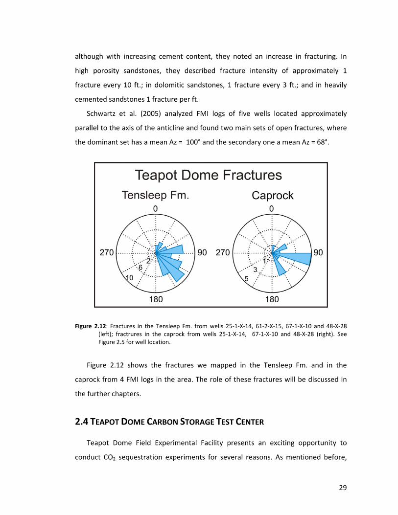
Table 2.2: Data types and format at Teapot Dome ……………………………….….…………... 31
Table 2.3: Summary of Tensleep wells with most complete data set in Section 10 … 32
Table 3.1: Parameters and data needed to define the stress tensor and the
geomechanical model ……………….………………………………….…………………………. 44
Table 4.1: Porosity and Permeability values from Yin’s lithofacies analysis ………….… 71
Table 4.2: Porosity and Permeability values from core plugs from 8 wells in
Section 10 ………………………………………………………………………………………………….. 72
Table 4.3: Basic reservoir and fluid data…………………………………………………………………. 81
Table 4.4: Six‐component EOS definition .………………………………..........………………….… 90
Table 4.5: Parameters of the three case scenarios used in the history matching
sensitivity analysis …………………………………………………………….……………………….. 92
Table 4.6: Sensitivity analysis on some History Matching parameters compared
against Scenario I …………………………………………………………………………….…….... 93
Table 4.7: Sensitivity analysis on some History Matching parameters compared
against Scenario II …………………………………………………………………….……………… 94
Table 4.8: Sensitivity analysis of relative permeability curves (Krel) compared with
Scenario III …………………………………………………………………………….………………….. 98
xvi
Table 4.9: Properties of the Base Case Scenario ………………………………………………….. 100
Table 4.10: Percentage of oil recovered in each of the cases compared to primary
injection without CO2 ………………………………………………………………………….…… 106
Table 4.11: Percentage of oil recovered in each of the cases with well control
strategy compared to primary injection without CO2 ………………….…………… 108
Table 4.12: CO2 emissions from power plants in the US ………………………………………. 109
Table 4.13: Summary of simulations to test the Tensleep Fm. storage capacity …… 110
Table 4.14: Effect of fracture permeability in oil recovery compared to the BC after 6
and 12 weeks, and 5 years of 1 MMcfd CO2 injection …………………..………….. 112
Table 4.15: Effect of fracture spacing on oil recovered compared to the BC after 6
and 12 weeks, and 5 years of 1 MMcfd CO2 injection …………………………….… 113
Table 4.16: Effect of Krel curves on oil recovered compared to the BC after 6 and 12
weeks, and 5 years of 1 MMcfd CO2 injection …………………………………….……. 114
Table 5.1: Total number of fractures mapped from the FMI logs in each of the
wells …….………………………………………………………………………………………………... 147
Table 5.2: Summary of observations in different areas surrounding the wells ….…. 161
Table 5.3: Summary of observations in different areas surrounding the wells …….. 162
xvii
LIST OF FIGURES
NUMBER PAGE
Figure 2.1: Stabilization wedges .…………………………………………………………………………… 10
Figure 2.2: Location of Teapot Dome …………………………………………………………………… 14
Figure 2.3: E‐W cross section with major reverse faults ……………………………………….. 17
Figure 2.4: NW‐SE cross section through Teapot Dome ……………………………………….. 18
Figure 2.5: Time structure map of the Tensleep Fm. ………………………………………….... 18
Figure 2.6: Time structure map of the Tensleep Fm. ………………………………………….….. 20
Figure 2.7: Time structure map of the 2nd Wall Creek member …………….……………… 21
Figure 2.8: Stratigraphic column of Teapot Dome ………………….………………….………… 22
Figure 2.9: Paleogeographic map of Early Permian Tensleep extent ……………………… 25
Figure 2.10: Schematic stratigraphic column of reservoir (Tensleep Fm.) and caprock
(Goose Egg Fm.) ……………………………………………………………………………………….… 26
Figure 2.11: Core description, environmental interpretation, and sequence‐
stratigraphic architecture of Tensleep well 54‐TPX‐10 from within
Section 10 …………………………………………………………………………………………..……. 27
Figure 2.12: Fractures in the Tensleep Fm. ……………………………………………………..…….. 29
xviii
Figure 2.13: Study Area with location of wells ……………………………………..……………….. 32
Figure 2.14: Existing carbon dioxide infrastructure in the region …………………………… 34
Figure 3.1: Location of Teapot Dome ……………………………………………..……………………… 39
Figure 3.2: NW‐SE cross section through Teapot Dome ……………………………….……….. 40
Figure 3.3: Time‐structure map in milliseconds (ms) of Tensleep Formation in Section
10 showing SHmax direction …………………………………………………………………………. 42
Figure 3.4: Observations of drilling‐induced tensile fractures …………………………..…... 45
Figure 3.5: Stress polygon for well 67‐1‐X‐10 …………………………………………………..……. 47
Figure 3.6a: Fault surface color‐coded with critical pressure perturbation values
indicating the fault slip potential .…..……………………………………………………..... 49
Figure 3.6b: Fault surface color‐coded with critical pressure perturbation values
indicating the fault slip potential considering the poro‐elastic effect .…........ 51
Figure 3.7: Fault slip potential probability for Normal Fault environment ……………… 52
Figure 3.8: Fault slip potential probability for Strike‐Slip environment ……..…………… 53
Figure 3.9: Fault slip potential probability as function of variation in the fault azimuth
and dip angle …….…………………………………………………………………..……..…………… 54
Figure 3.10: Strike orientation of main fractures sets in the Tensleep Fm. ………….…. 56
Figure 3.11: Rose diagrams of the dominant fracture sets at the Tensleep Fm. …….. 57
Figure 3.12: Fractures sets mapped in three FMI well logs in the S1 area ……………... 58
Figure 3.13: Observed Tensleep Fm. and caprock fractures ……………………………..……. 58
Figure 3.14: Time‐structure map in milliseconds (ms) of the 2nd Wall Creek showing
SHmax directions ………………………………………………………………………………………….. 60
Figure 3.15: S2 fault surfaces color‐coded with critical pressure perturbation values
indicating the fault slip potential ………………………….……………….……………..……. 61
Figure 4.1: Schematic stratigraphic column of reservoir and caprock ………...….….… 67
Figure 4.2: Depth‐structure map of the Tensleep Fm. …………………………………………... 69
Figure 4.3: 3D Upscaled grid ……………………………………………………………………….…………. 70
Figure 4.4: Example of porosity and permeability geostatistical distribution for
A‐Sand and upper B‐Sand intervals …………………………..……………………………….. 72
xix
Figure 4.5: Map showing one of the permeability realizations at the B‐Sandstone
and B‐Dolostone levels ………….…………………………………………………………….….… 73
Figure 4.6: SSW – NNE Cross section of upscaled grid ……………………………………………. 74
Figure 4.7: Map of the upscaled grid showing one of the permeability realizations at
the B‐Sandstone and B‐Dolostone levels …………………………….……………….….… 74
Figure 4.8: Illustration of typical CO2 Flood designs …………………………………………….…. 79
Figure 4.9: Historic oil and water production from Tensleep Fm. at Teapot Dome,
from 1959 – 2008 ………………………………………………………………………………….…… 82
Figure 4.10: Water‐oil relative permeability curves as a function of water saturation
measured in four Tensleep samples ……………………………………….……………….. 84
Figure 4.11a: Water‐oil relative permeability curves, from Sample A, used in the
base case scenario as a function of water saturation …………………………………. 85
Figure 4.11b: Gas‐oil relative permeability curves, from Sample A, used in the
base case scenario as a function of water saturation …………………………………. 85
Figure 4.12: Laboratory and average capillary pressure curves ……………………..………. 88
Figure 4.13: Analysis of Tensleep Fm. oil samples …………………………………………..…….. 89
Figure 4.14: History matching sensitivity to grid size …………………………………………….. 93
Figure 4.15: History matching sensitivity to fracture permeability ………………………... 95
Figure 4.16: History matching sensitivity to fracture porosity ……………………………….. 95
Figure 4.17: History matching sensitivity to fracture spacing ..…………………………….. 96
Figure 4.18: History matching sensitivity to initial water saturation ………………….….. 97
Figure 4.19: History matching sensitivity to capillary pressure ..…………………………….. 98
Figure 4.20: History matching sensitivity to relative permeability curves ………………. 99
Figure 4.21: Comparison between the base case scenario and field data ………….… 101
Figure 4.22: Cumulative water at surface conditions (SC) of base case scenario
and field data ……………………………………………………………………………..……………. 101
Figure 4.23: Injector set up …………………………………………………………….………………….. 103
Figure 4.24: Gas Saturation in the fractures after 6 weeks of injection …………….. 104
Figure 4.25: Base Case: Injection of 1 MMcfd of CO2 for 6 weeks. Oil rate at
xx
surface conditions ……………………………………………………………………………..……. 105
Figure 4.26: Base Case: Injection of 1 MMcfd of CO2 for 6 weeks. Gas saturation in
fractures ………………………………………………………………………………………………………..……. 105
Figure 4.27: Oil rate in each of the cases as well as primary production without
CO2 ………………………………………………………………………………………………………….107
Figure 4.28: Incremental oil recovery of each of the cases, with a well control
strategy ………………………………………………………………………………….………………… 108
Figure 4.29: injection of 1 MMcfd in 2 and 3 simultaneous injectors as well as 2
MMcfd in 1, 2 and 3 injector ………………………………………..………………………….. 111
Figure 4.30: Average Krel curves described by Gaviria (2005) ……………………………….. 114
Figure 4.31: Oil rate comparison between BC and a case run with a different matrix
porosity and permeability distribution ………………………………………..…………… 115
Figure 4.32: Cumulative Oil comparison between BC and 10, 4, 2, 0.5, and 0.25 times
the original fracture permeability ………………………………………………………….... 117
Figure 4.33: Cumulative Oil comparison between BC and four different relative
permeability curves ..………………….………………………………………………………….... 117
Figure 4.34: Cumulative Oil comparison between BC and 10, 4, 2, 0.5, and 0.25 times
the original fracture spacing ………………………………………………………………….... 118
Figure 4.35: Cumulative Oil comparison between BC and 10, 4, 2, 0.5, and 0.25 times
the original fracture porosity ………………………………………………………………...... 118
Figure 4.36: Cumulative Oil comparison between BC and 10 simulations with
different realizations of matrix permeability (Yin’s analysis) .…………………... 119
Figure 4.37: Cumulative Oil comparison between BC and 10 simulations with
different realizations of matrix porosity (Yin’s analysis) …………………………... 120
Figure 4.38: Cumulative Oil comparison between BC and 10 simulations with
different realizations of matrix permeability (core values) ….…………………... 119
Figure 4.39: Cumulative Oil comparison between BC and 10 simulations with
different realizations of matrix porosity (core values) ……..….…………………... 119
Figure 5.1: Incidence and azimuthal angles & HTI medium ………………………………… 129

xxi
Figure 5.2: Rüger's model compared to amplitudes of a real seismic gather ……… 130
Figure 5.3: Time‐structure map of Tensleep B showing location of the wells …..….. 132
Figure 5.4: Rose diagrams of Tensleep Fm. fractures …………………………………….…….. 133
Figure 5.5: Rose diagrams of Opeche fractures …………………………………………….…….. 133
Figure 5.6: Time‐structure map of Tensleep B showing the structural framework of
the Tensleep Fm. ……………………………………………………………………………………… 134
Figure 5.7: Azimuth of the anisotropy at the top of the Tensleep …….…………………. 136
Figure 5.8: Azimuth of the anisotropy at the top of the TensleepB ……………………... 137
Figure 5.9: Azimuth of the anisotropy at the top of the caprock ….………………………. 138
Figure 5.10: Angular histogram of Anisotropy Azimuth in the three horizons ……… 139
Figure 5.11: Tensleep Anisotropy around well 25‐1‐X‐14 …………………………………….. 140
Figure 5.12: Comparison of AVAZ anisotropy azimuths with stress fracture and fault
orientation from seismic and well data around well 25‐1‐X‐14 ………………… 141
Figure 5.13: Tensleep Anisotropy around well 61‐2‐X‐15 …………………………………….. 142
Figure 5.14: Comparison of AVAZ anisotropy azimuths with stress fracture and fault
orientation from seismic and well data around well 61‐2‐X‐15 ………………… 142
Figure 5.15: Tensleep Anisotropy around well 67‐1‐X‐10 …………………………………….. 143
Figure 5.16: Comparison of AVAZ anisotropy azimuths with stress fracture and fault
orientation from seismic and well data around well 67‐1‐X‐10 ………………… 143
Figure 5.17: Tensleep Anisotropy around well 71‐1‐X‐4 ………..…………………………….. 144
Figure 5.18: Comparison of AVAZ anisotropy azimuths with stress fracture and fault
orientation from seismic and well data around well 71‐1‐X‐4 ……..…………… 145
Figure 5.19: Tensleep Anisotropy around well 48‐X‐28 …….…..…………………………….. 146
Figure 5.20: Comparison of AVAZ anisotropy azimuths with stress fracture and fault
orientation from seismic and well data around well 48‐X‐28 ……..…….……… 146
Figure 5.21: TensleepB Anisotropy around well 25‐1‐X‐14 …………………………………. 148
Figure 5.22: Comparison of AVAZ anisotropy azimuths with stress fracture and fault
orientation from seismic and well data around well 25‐1‐X‐14 ………………… 148
Figure 5.23: TensleepB Anisotropy around well 61‐2‐X‐15 ………………………………….. 149

xxii
Figure 5.24: Comparison of AVAZ anisotropy azimuths with stress fracture and fault
orientation from seismic and well data around well 61‐2‐X‐15 ………………… 149
Figure 5.25: TensleepB Anisotropy around well 71‐1‐X‐4 ………..………………………….. 150
Figure 5.26: Comparison of AVAZ anisotropy azimuths with stress fracture and fault
orientation from seismic and well data around well 71‐1‐X‐4 ……..…………… 150
Figure 5.27: TensleepB Anisotropy around well 48‐X‐28 …….….………………………….. 151
Figure 5.28: Comparison of AVAZ anisotropy azimuths with stress fracture and fault
orientation from seismic and well data around well 48‐X‐28 ……..…….……… 151
Figure 5.29: Opeche Anisotropy around well 25‐1‐X‐14 ……..……………………………….. 153
Figure 5.30: Comparison of AVAZ anisotropy azimuths with stress fracture and fault
orientation from seismic and well data around well 25‐1‐X‐14 ………………… 153
Figure 5.31: Opeche Anisotropy around well 61‐2‐X‐15 …………..………………………….. 154
Figure 5.32: Comparison of AVAZ anisotropy azimuths with stress fracture and fault
orientation from seismic and well data around well 61‐2‐X‐15 ………………… 154
Figure 5.33: Opeche Anisotropy around well 67‐1‐X‐10 ………..…………………………….. 155
Figure 5.34: Comparison of AVAZ anisotropy azimuths with stress fracture and fault
orientation from seismic and well data around well 67‐1‐X‐10 ………………… 155
Figure 5.35: Opeche Anisotropy around well 71‐1‐X‐4 ………..………..…………………….. 156
Figure 5.36: Comparison of AVAZ anisotropy azimuths with stress fracture and fault
orientation from seismic and well data around well 71‐1‐X‐4 ……..…………… 156
Figure 5.37: Opeche Anisotropy around well 48‐X‐28 …….…..…………..………………….. 157
Figure 5.38: Comparison of AVAZ anisotropy azimuths with stress fracture and fault
orientation from seismic and well data around well 48‐X‐28 ……..…….……… 157
Figure 5.39: Bedforms structure and dimensions of the Entrada Sandstone ……….. 158
Figure 5.40: Amplitude time‐slice at the depth of the Tensleep Fm. ……………………. 159
Figure 5.41: Amplitude time‐slice showing the acquisition pattern of the Teapot
Dome 3D seismic volume …………………………………………………………………………. 160
Figure 6.1: Satellite image of Michigan area with location of test site ……………….… 167
Figure 6.2: Stratigraphic column of the test site ………………………………………………….. 169
xxiii
Figure 6.3: Structural map of Bass Island dolomite in Michigan ……………..……………. 170
Figure 6.4: Regional Stratigraphic cross section …………………………………….…………….. 171
Figure 6.5: Distribution of tensile fractures in well State Charlton 4‐30 ………………. 173
Figure 6.6: Regional Stress map ……………………………………………………….………………….. 174
Figure 6.7: Stress summary plot …………………………………………………………………………… 175
Figure 6.8: 200x200x5 grid of the BILD ……………………………………………….……………….. 176
Figure 6.9: Porosity and permeability values from core samples …………………….…... 177
Figure 6.10: Total CO2 [m3] and CO2 injection rate [m
3/day] over ten years ………… 178
Figure 6.11: Detail of BILD grid with CO2 saturation after 10 year of injection …..… 178
Figure 6.12: Detail of BILD grid showing formation pressure after 10 year of
injection ………………………………………………………………………………………………..… 179
Figure 6.13: Map of experiment setup …………………………………………………….…………. 180
Figure 6.14: Depth profile of microseismic monitoring set up setup …………………. 180
Figure 6.15: Injection rate, well head pressure and daily seismicity rate ……………... 181
1
CHAPTER 1
INTRODUCTION
1.1 OVERVIEW AND MOTIVATION
There is increasing evidence that reinforces the view that climate and greenhouse
gas cycles are intimately related. CO2 is the main anthropogenic gas contributing to
the greenhouse effect and global warming, and there is no evidence at any time in
the past 650,000 years of levels of carbon dioxide as high as the current atmospheric
concentrations (Brook, 2005). CO2 levels are a third higher than in pre‐industrial
times, and are projected to increase at 0.4% per year.
The main anthropogenic source of CO2 is the burning of fossil fuels which
currently dominate commercially supplied energy worldwide. Since it is generally
accepted that concentration in the atmosphere of greenhouse gases, in particular
CO2, must be restricted, several solutions have been proposed to try to stabilize
carbon dioxide concentrations that include carbon capture and storage (CCS).
Nevertheless, for CCS to be a viable carbon management solution, one of the main
issues to be addressed is the risk of CO2 leakage.
2
This thesis is composed of four interrelated investigations that focus on the
geomechanical aspects of carbon storage with emphasis on the assessment of the
leakage risks. Three of these studies analyze a CO2‐EOR and Sequestration project
planned for the fractured Tensleep Formation at Teapot Dome Oil Field, WY. While
the fourth one investigates the use of induced microseismicity as a tool to enhance
permeability and monitor sequestration projects in a deep saline formation in the
Michigan Basin.
The first study consist of the geomechanical characterization at Teapot Dome; its
goal is to understand the effect that CO2 injection will have in fault stability and seal
integrity to ultimately predict the potential risk of CO2 leakage through natural
pathways. The second study develops of a stochastic reservoir model of the Tensleep
Fm. and a fluid flow simulation to model the migration of the injected CO2 as well as
to obtain limits on the rates and volumes of CO2 that can be injected without
compromising seal integrity. The third project describes an Amplitude Versus Angle
and Azimuth (AVAZ) analysis performed at Teapot Dome to identify the presence of
fractures using wide‐azimuth 3D seismic data. The objective of the this analysis is to
expand the 1D scattered fracture characterization performed from four wells in the
anticline to a 3D characterization of the fracture network on both the reservoir and
the caprock that will allow for a more accurate assessment of the impact of these
fractures in reservoir permeability and in the risk of CO2 leakage.
From a technical perspective, depleted or mature oil and gas reservoirs hold great
promise as sequestration sites because they have hold hydrocarbons for geological
periods of time, implying the presence of effective trap and seal mechanisms.
However, it has long been recognized (e.g., Raleigh et al. 1976) that fluid injection
causes changes in the pore pressure and stress field that could potentially alter the
initial seal of the reservoir by either hydraulically fracturing the cap rock or triggering
slip on pre‐existing faults by reducing the effective normal stress on the fault plane
(see review by Grasso, 1992).
3
In light of this, a key step in the evaluation of any potential site being considered
for geologic carbon sequestration is the ability to predict whether the increased
pressures associated with CO2 sequestration are likely to affect seal capacity. To that
end, the last study consists in the analysis of an injection‐induced microseismicity
experiment in the Bass Island Dolomite (BILD) in the Michigan Basin. One of the
biggest challenges for CO2 sequestration in deep saline formations is the very low
porosity and permeabilities often shown that translates into limited injectivity and
storage capacities. Injection‐induced microseismicity has been frequently used in the
oil industry to enhance permeability. Microseismic stimulation is initiated by
increasing the fluid pressure in the target formation, thus reducing the effective
normal stress on optimally‐oriented faults and fractures triggering slip and creating
high‐permeability paths within the reservoir. The induced failure is mainly triggered
by a diffusive process of pore pressure perturbation and often occurs as a sequence
of many small events. The volume of rock stimulated can be imaged by locating these
microearthquakes induced by the injection (Albright and Pearson, 1982) therefore
constituting an excellent monitoring technique.
1.2 THESIS OUTLINE
This thesis is composed of six chapters. Chapter 1 is the present Introduction.
Chapters 2, 3, 4 and 5 are related with the Teapot Dome investigations and Chapter 6
describes the microseismicity experiment in the Michigan Basin.
In Chapter 2, Teapot Dome Oil Field – National Geological Carbon Storage Test
Center, I present an overview of the Teapot Dome geology and history and the
characteristics of the Carbon Storage Test Center. The planned CO2‐EOR and
sequestration pilot is described as wells as the source for the injected CO2.
In Chapter 3, Seal Integrity and Feasibility of CO2 Sequestration in the Teapot
Dome EOR Pilot: Geomechanical Site Characterization, I present the geomechanical
characterization performed at Teapot Dome to establish the potential risk of leakage
4
due to CO2 injection. The first part of the chapter focuses on the S1 fault area and the
Tensleep Fm., characterizing fault stability and seal integrity to establish the
feasibility of the CO2‐EOR and Sequestration pilot. This manuscript was published in
the June 2008 issue of Environmental Geology (v.54, no. 8). The rest of the chapter
completes the analysis with a fracture characterization on the Tenlseep and the
caprock and the evaluation of the effect of these features on reservoir permeability
along with their potential risk of reactivation and becoming pathways for CO2 leakage.
Finally, the S2 fault area at the depth of the 2nd Wall Creek member is evaluated as
the target of a controlled CO2 leakage experiment.
In Chapter 4, 3D Stochastic Reservoir Model and Reservoir Simulation of the
Tensleep Fm., I combine the previous geomechanical analysis, geostatistical reservoir
modeling and fluid flow simulations to model the migration of the injected CO2 as
well as to obtain limits on the rates and volumes of CO2 that can be injected without
compromising seal integrity. The CO2‐EOR pilot was modeled and the storage
capacity of the Tensleep in this particular trap was assessed. Finally, a sensitivity
analysis was conducted to estimate the response of the pilot performance to several
parameters such as fracture permeability, porosity and spacing, relative permeability
curves, matrix porosity and permeability, and grid size.
In Chapter 5, Fracture Detection Using Amplitude Versus Angle and Azimuth at
Teapot Dome Oil Field, WY, I describe an analysis performed at Teapot Dome to
identify the presence of fractures using wide‐azimuth 3D seismic data. This project is
the result of collaboration with David Gray from CCGVeritas, Canada. David Gray was
in charge of the AVAZ processing, and I provided the geomechanical and fracture
characterization obtained in Chapter 3, as well as the interpretation of the results.
From the AVAZ analysis, anisotropy direction and magnitudes were obtained. I
analyzed and calibrated them with stress, fractures, fault, and sedimentary data from
wells and seismic interpretation to try to determine if the origin of the anisotropy
could be related to the stress state, the structural framework or to a sedimentary
control. The results from the AVAZ analysis are extremely variable, and at this point,

5
there is no conclusive evidence to discriminate which of these factors is primarily
affecting the observed anisotropy. Furthermore, it is possible that the method does
not work with this data set, because particularities of this setting do not follow the
assumptions of the method.
In Chapter 6, Using Microseismic Stimulation to Enhance Permeability in Tight
Formations, I present a preliminary geomechanical characterization and fluid flow
simulation performed as a base for an Induced Microseismicity Experiment in the
Bass Island Dolomite (BILD) in the Michigan Basin. The original objectives of this
experiment were to enhance permeability and injectivity in a tight deep saline
formation, a target for a CO2 sequestration pilot. A further objective was to test
microseismicity as a monitoring technique in the carbon sequestration context.
During the experiment a total of ~10,000 metric tons of supercritical CO2 were
injected into the BILD over a period of 40 days. The passive seismic monitoring
started 16 days prior to the start of injection and ended after 47 days of operation.
The last part of the chapter describes the microseismicity data processing and
analysis led by Dr. Marco Bohnhoff, currently a visiting professor at Stanford. I
participated in this process helping to analyze waveforms, picking wave onsets and
performing a frequency and filtering analysis. The results form this work will be
published, where I will be the second author after Bohnhoff.
6
CHAPTER 2
TEAPOT DOME OIL FIELD – NATIONAL
GEOLOGICAL CARBON STORAGE TEST
CENTER
2.1 ABSTRACT
Mature oil and gas reservoirs are attractive targets for geological sequestration of
CO2 because of their potential storage capacities and the possible cost offsets from
enhanced oil recovery (EOR).
The Teapot Dome Field Experimental Facility presents an exciting opportunity
to conduct CO2 sequestration experiments since it is fully owned by the US
government, and this Federal ownership grants a stable platform for long‐term

7
scientific investigations in a steady business context, absent the commercial drivers
of a privately owned oil field. Furthermore, the extensive data set of Teapot Dome as
well as any experimental result is public domain. This framework allows joint
research of all kinds (Friedmann et al., 2004b).
A CO2‐EOR and Sequestration Pilot is projected to start at Teapot Dome, early in
2009, targeting the Pennsylvanian Tensleep Formation. The objective is to test the
EOR and sequestration potential of the Tensleep in the area denominated Section 10.
In this chapter we will describe the proposed pojects related to CO2 sequestration
that we investigated throughout this dissertation. We will also present the geology
and the characteristics of Tapot Dome, as well as the available data set.
2.2 INTRODUCTION
2.2.1 GREENHOUSE EFFECT, CLIMATE CHANGE, AND CO2 EMISSIONS
Human activity in the last 200 years has caused considerable changes in the levels
of several atmospheric greenhouse gases, including carbon dioxide (CO2). These
changes are particularly noticeable since the industrial revolution. Although direct
measurements began in the latter half of the 20th century, atmospheric
concentration of these gases from earlier times are known from coring samples of
polar ice (Petit et al., 1999, Siegenthaler et al., 2005). This data highlights the fact
that at no time in the past 650,000 years were carbon dioxide or methane (CH4)
levels significantly higher than values just before the Industrial Revolution (Brook,
2005). Similarly, it also points out the evident co‐variation of CO2 and CH4 with
climate cycles (Brook, 2005, Falkowski et al., 2000). This relationship reinforces the
view that climate and greenhouse gas cycles are intimately related. Although the
exact effect of how greenhouse gases will change the climate is still uncertain, a rise
in the global average temperature, or global warning, is expected.
8
The primary greenhouse gas produced by human activity is CO2 with a current
atmospheric concentration of 383.9 ppm (Blasing, 2008), approximately a third more
since pre‐industrial times. It continues to increase at 0.4% per year (IEA Greenhouse
Gas R&D Programme, 2005).
The main anthropogenic source of CO2 comes from the burning of fossil fuels
such as oil, coal and natural gas, around 23.5 ‐ 31.3 Gt CO2 (6 ‐ 8 GtC) per year
(Parson & Keith, 1998, & IEA Greenhouse Gas R&D Programme, 2001). In addition,
changes in tropical land use, such as deforestation by forest burning, contribute
about a quarter of the effect of fossil fuels. For these reasons, it is now generally
accepted that concentration in the atmosphere of greenhouse gases, in particular
CO2, must be restricted. Several scenarios have been proposed in the so called
“pathway to stabilization” to steady CO2 concentrations from 450 to 750 ppm (Beecy
and Kuuskraa, 2001).
Several techniques have been proposed in this pathway, such as to reduce
consumption of energy services, increase energy efficiency, switch to lower carbon‐
content fuels, enhance CO2 sinks (forests, soils and oceans), use energy sources with
very low CO2 emission (renewable energy or nuclear energy) and capture and storage
of CO2 (IEA Greenhouse Gas R&D Programme, 2001). The use of each of these
techniques will depend on several factors, including emission‐reduction target costs,
available energy resources, environmental impact and social factors. However none
of them is sufficient by itself (Beecy and Kuuskraa, 2001), and all of them will take
time to be ready to implement.
Among those alternatives, underground CO2 sequestration is an attractive option
to pursue because it can be applied in the short‐term, with available technology
developed mainly in the oil and gas industry. This approach becomes even more
attractive when we consider that currently around 85% of the world’s commercial
energy needs are supplied by fossil fuel. Therefore, a technique capable of reducing
the CO2 emissions, while still using fossil‐fuel based energy, could be of crucial help

9
to avoid the significant disturbance that a rapid change of non‐fossil energy sources
could cause (IEA Greenhouse Gas R&D Programme, 2001).
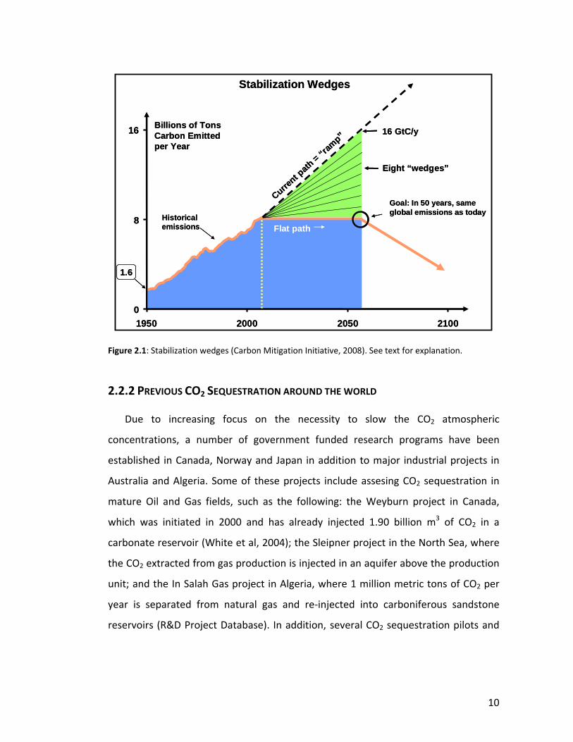
Pacala and Socolow (2004) defined the concepts of stabilization triangle and
stabilization wedges (Figure 2.1). The stabilization triangle represents the desired
amount of CO2 emission reduction in 50 years. It is the difference between the
projection of the current carbon emission path and a flat path at the current carbon
emission rate. This triangle is divided in wedges, where each wedge coresponds to a
strategy to reduce carbon emissions that grow in 50 years from zero to 1.0 GtC/yr. A
requisit for all strategies is that they have to be already commercialized.
Carbon capture and storage (CCS) has been proposed as one of these strategies.
There are currently three sequestration projects worldwide, each of which inject ~1
million tons of CO2 per year. In order for this technology to became a solution to the
CO2 problem, at least 3500 such projects must be in place by 2055 (Carbon Mitigation
Initiative, 2008).
To have an idea of the urgency of the problem, when this concept was developed
in 2004, seven wedges were defined. Currently, already eight wedges form the
stabilization triangle.
10
Figure 2.1: Stabilization wedges (Carbon Mitigation Initiative, 2008). See text for explanation.
2.2.2 PREVIOUS CO2 SEQUESTRATION AROUND THE WORLD
Due to increasing focus on the necessity to slow the CO2 atmospheric
concentrations, a number of government funded research programs have been
established in Canada, Norway and Japan in addition to major industrial projects in
Australia and Algeria. Some of these projects include assesing CO2 sequestration in
mature Oil and Gas fields, such as the following: the Weyburn project in Canada,
which was initiated in 2000 and has already injected 1.90 billion m3 of CO2 in a
carbonate reservoir (White et al, 2004); the Sleipner project in the North Sea, where
the CO2 extracted from gas production is injected in an aquifer above the production
unit; and the In Salah Gas project in Algeria, where 1 million metric tons of CO2 per
year is separated from natural gas and re‐injected into carboniferous sandstone
reservoirs (R&D Project Database). In addition, several CO2 sequestration pilots and
1.6
Billions of Tons Carbon Emitted per Year
Current p
ath = “r
amp”
Historicalemissions Flat path
0
8
16
1950 2000 2050 2100
Stabilization Wedges
16 GtC/y
Eight “wedges”
Goal: In 50 years, sameglobal emissions as today
1.6
Billions of Tons Carbon Emitted per Year
Current p
ath = “r
amp”
Historicalemissions Flat path
0
8
16
1950 2000 2050 2100
Stabilization Wedges
16 GtC/y
Eight “wedges”
Goal: In 50 years, sameglobal emissions as today
11
demos are currently in place (30 Mt CO2 per year) as well as CO2 enhanced oil
recovery (EOR) applications.
The majority of the EOR projects are located in Texas, USA, where this technology
started in the early 1970s. Presently, most of the CO2 used in such applications comes
from natural reservoirs in the western US, but a portion of it comes from
anthropogenic sources such as natural gas processing plants (Gale, 2004 & IPCC,
2005).
2.2.3 CO2 SEQUESTRATION UNDERGROUND – STORAGE OPTIONS
Several factors suggest that geologic storage of CO2 underground is a viable
alternative that can be implemented with techniques similar to those used in the oil
and gas industry. Natural analogues, such as oil and gas, as well as CO2, fields
demonstrate that fluids have been stored and preserved underground for millions of
years. Successful industrial analogues include natural gas storage projects, liquid
waste disposal projects and CO2 sequestration or CO2‐EOR projects such as Sleipner
and Weyburn, where positive outcomes are anticipated through monitoring projects.
According to the IPCC report (September 2005) geological storage of CO2 can
make a substantial impact on carbon dioxide emission reduction. The main proposed
options to store CO2 underground are saline reservoirs, unminable coal beds, and
mature oil and gas reservoirs.
My research focuses mainly on mature oil and gas fields (O&G), where the upper
estimate of storage capacity could account for approximate 45% of global emissions
for the year 2050 (IEA Greenhouse Gas R&D Programme, 2001). Parson & Keith
(1998) estimated the global capacity of depleted Oil and Gas fields in between ~740 –
1850 Gt CO2 (~200 to 500 GtC). However, this estimate should be considered
theoretical, because geographical relationships between large emission sources and
storage reservoirs have to be evaluated (Gale, 2004). Geological CO2 sequestration is
considered a short‐term solution, and in order to have a real impact, the
12
sequestration rates have to be approximately one third of projected global oil
production rates, which is highly ambitious. However, if these rates can be met while
the impact of potential leakags is minimized, then the practice of sequestration can
be publicly acceptable.
2.2.4 CO2 SEQUESTRATION IN MATURE OIL & GAS FIELDS
In addition to their potential capacities, mature O&G reservoirs are an attractive
target for sequestration because of potential cost offsets from enhanced oil recovery
(EOR) using CO2, which is current practice in the oil industry. However, mainly due to
economic and regulatory characteristics, these applications are typically designed to
obtain maximum oil production with minimum CO2 injection (GEO‐SEQ Best Practice
Manual 2004). For the opposite scenario to exist, in which a maximum quantity of
CO2 were to remain in the reservoir while still increasing production, some type of
financial incentive (tax credits or emission trading) must be present for the operator.
Until then, this ideal scenario is considerably different from conventional EOR
projects.
O&G reservoirs also present some advantages compared to saline aquifers and
unminable coal beds due to the exploration and development activities that they
have undergone. These fields have the entire production infrastructure in place,
fewer regulatory barriers could be encountered, and they present an extensive
knowledge base accumulated since the early exploratory stages of the field. Large
volumes of fluids were stored for geologic periods of time, which implies that
adequate seal capacities, porosity and permeabilities existed at one time.
2.2.5 RISK OF LEAKAGE DURING CO2 SEQUESTRATION
One of the main problems of CO2 sequestration underground is the risk of global
and local CO2 leakage. The term global leakage refers to the scenario where CO2
13
make its way out to the atmosphere canceling the sequestration effect, and local
leakage refers to the impact that the CO2 will cause to people and ecosystems in the
surroundings of the injection sites, i.e. contamination of drinking water and ground
concentrations of CO2 (> 10% concentration is toxic) (Socolow, 2005). Therefore, a
full understanding of leakage and the ability to predict it is one of the key steps
towards the implementation of this technique through the design of effective risk
management strategies.
It has been established that the most dangerous leakage path in a depleted oil
and gas field is the numerous abandoned wells, however, the study of this process is
beyond the scope in this research. Here I focus on another important leakage
condouits which are the so called natural pathways, i.e. faults and fractures. I
evaluate the effect of CO2 injection on fault stability and seal integrity with the
objective of making predictions of the potential leakage risk through such pathways.
2.3 TEAPOT DOME
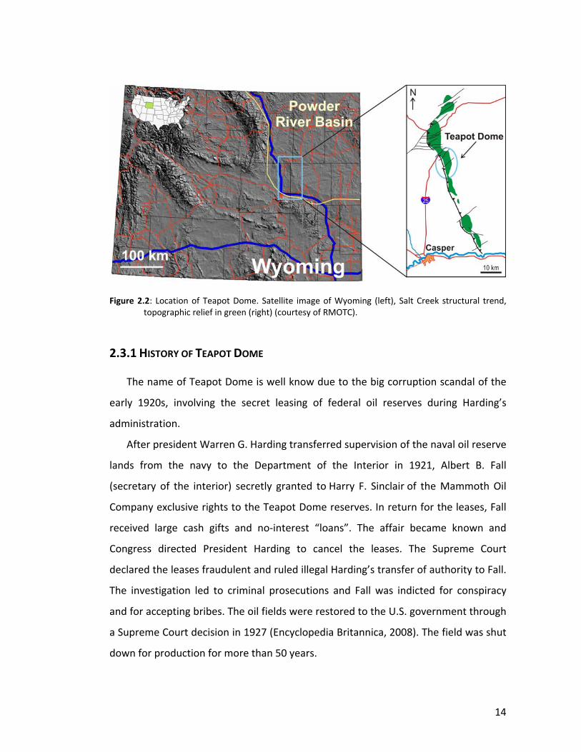
Teapot Dome is an elongated asymmetric, basement‐cored anticline with a north‐
northeast axis located in the southwestern edge of the Powder River Basin (Figure
2.2). It is part of the Salt Creek structural trend, with Salt Creek anticline to the north
and Sage Spring Creek and Cole Creek oil fields to the south (Beinkafner, 1986,
Cooper & Goodwin, 1988 and Cooper et al, 2001).
14
Figure 2.2: Location of Teapot Dome. Satellite image of Wyoming (left), Salt Creek structural trend,
topographic relief in green (right) (courtesy of RMOTC).
2.3.1 HISTORY OF TEAPOT DOME
The name of Teapot Dome is well know due to the big corruption scandal of the
early 1920s, involving the secret leasing of federal oil reserves during Harding’s
administration.
After president Warren G. Harding transferred supervision of the naval oil reserve
lands from the navy to the Department of the Interior in 1921, Albert B. Fall
(secretary of the interior) secretly granted to Harry F. Sinclair of the Mammoth Oil
Company exclusive rights to the Teapot Dome reserves. In return for the leases, Fall
received large cash gifts and no‐interest “loans”. The affair became known and
Congress directed President Harding to cancel the leases. The Supreme Court
declared the leases fraudulent and ruled illegal Harding’s transfer of authority to Fall.
The investigation led to criminal prosecutions and Fall was indicted for conspiracy
and for accepting bribes. The oil fields were restored to the U.S. government through
a Supreme Court decision in 1927 (Encyclopedia Britannica, 2008). The field was shut
down for production for more than 50 years.
15
Teapot Dome was reopened in 1976 and in 1977 became a US Department of
Energy (US DOE) facility. DOE directed RMOTC to collaborate with the petroleum
industry to improve domestic oil and gas production through the field testing of new
technology, and in October 2003, established Teapot Dome as a national geological
carbon storage test center (Friedmann et al., 2004a).
Regarding the production history, Teapot Dome started its production in 1908
from the “Dutch” well (200 BOPD) at the First Wall Creek sandstone In 1909 a few
more wells were drilled to develop the Shannon sandstone. Before the reopening of
the field and the development and exploration program at Teapot Dome in 1976, a
total of 233 wells had been drilled in all the producing formations. In 1996, additional
1007 development wells and 90 exploratory wells were drilled. 27 of the
development wells were drilled targeting the Tensleep Fm., and two of them
experienced the highest initial production rates of any wells in Wyoming at that time
(Gaviria, 2005).
2.3.2 REGIONAL GEOLOGY
Wyoming includes a large part of the Central Rocky Mountains and a smaller part
of the Southern Rocky Mountains, most of Wyoming basin province and a part of the
northern Great Plains. This situation positions Wyoming in a Phanerozoic tectonic
transition zone, extending from the flat rocks of the continental interior to the folded
and trusted strata of the Rocky Mountains (Snoke, 1993).
During early and middle Paleozoic times, central Wyoming was on the
northwestern flank of the Transcontinental Arch, a major basement high southwest‐
northeast trending, that influenced the depositional history of the Rocky Mountain
shelf. A considerable gap in the geologic record exists after mid‐Proterozoic until this
time. Therefore, early to mid Paleozoic shelf‐facies strata lay directly on top of
Precambrian basement. These deposits reflect a progressive west‐to‐east marine
transgression and are usually separated by disconformities due to relative changes in
16
the sea level. Late Paleozoic and early Mesozoic deposits also includes several
paleoenvironments such as paralic, eolian, and fluvial settings (Snoke, 1993,
Hennings et al, 2008).
In particular, a transgression period resulted in the deposition of the Amsden
Formation, which underlies the Tensleep and Phosphoria/Goose Egg Formations
(Hennings et al., 2008), the focus of the present work.
By mid‐Cretaceous until early Eocene occurred the thin‐skinned, fold‐and‐thrust
belt of the Sevier orogeny, one of the three overlapping events that have deformed
the west central US Cretaceous times. At the end of the Maastrichtian and during
Paleocene times, the Laramide orogeny produced a NE‐trending compression
(Dickinson and Snyder, 1978, Bird, 1989) east of the thin‐skinned thrusting of the
Sevier orogeny.
The Laramide orogeny formed basement‐cored uplifts separated by deep,
actively subsiding basins (Dickinson et al., 1988, Bird, 1989, Stone, 1993 and
Hennings et al., 2008). Teapot Dome is a typical example of a Laramide anticline, that
given its NW‐SE orientation it probably formed perpendicular to the Laramide
direction of compression (NE‐SW).
2.3.3 TEAPOT DOME ANTICLINE
Teapot Dome is a double–plunging asymmetrical anticline where the west flank
beds dip steeper (20 – 50°) than the east flank ones (<20°). It is bound on the west by
a main thrust fault, consisting probably of a series of high angle reverse faults (Figure
2.3) of approximate 35° to 40° east‐northeast, offsetting the Precambrian igneous
and metamorphic basement mapped in outcrop in adjacent ranges (McCutcheon,
2003, Friedmann and Stamp, 2006).
The anticline is compartmentalized in several blocks by major oblique strike‐slip
to normal faults (Figure 2.4 and 2.5) that have been assigned arbitrary names S1, S2,
S3, and S4 (McCutcheon, 2003). These faults are well defined in both the seismic data
17
and in the outcrops. They offset the basement and are oriented along a NE‐SW trend,
parallel to both the vergence direction of the main fold and basement foliation in
neighboring outcrops. Their orientation and complexity varies locally, but generally
have steep dips (Figure 2.4). At the surface, these faults have apparent lateral offsets,
and sub‐horizontal or oblique‐slip striations have been observed, thus they have
usually been interpreted as tear or accommodation faults (Cooper et al., 2003,
Friedmann et al., 2004 and Friedmann and Stamp, 2006). Friedmann and Stamp
(2006) noted that their timing appears to be coeval with Laramide shortening but
thickness changes across the faults in Paleozoic and Mesozoic strata suggest that
there were some earlier fault slip and growth strata events.
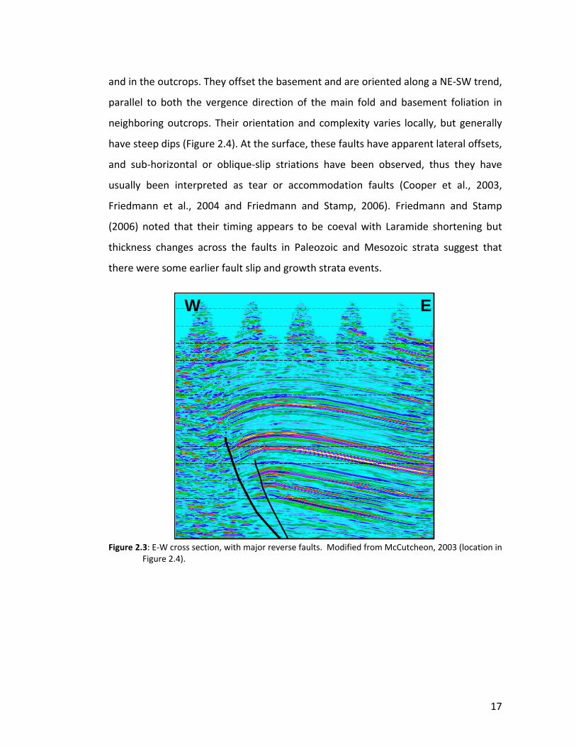
Figure 2.3: E‐W cross section, with major reverse faults. Modified from McCutcheon, 2003 (location in Figure 2.4).
W EW EW E
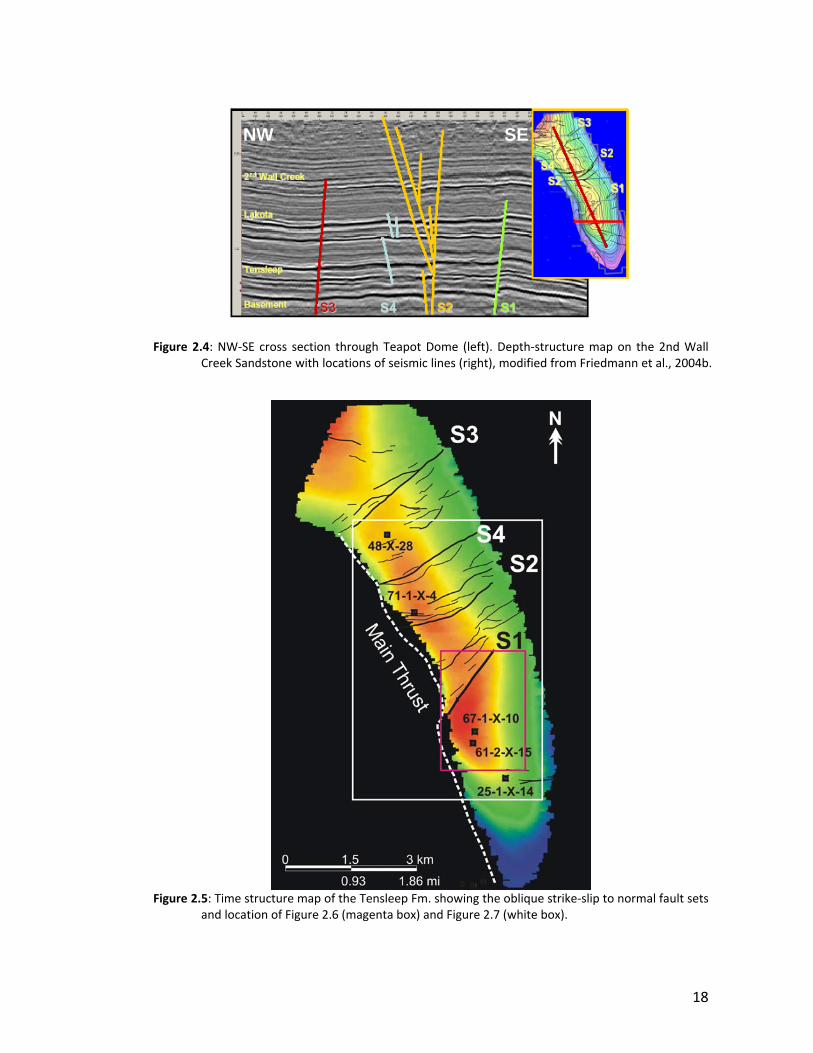
18
Figure 2.4: NW‐SE cross section through Teapot Dome (left). Depth‐structure map on the 2nd Wall
Creek Sandstone with locations of seismic lines (right), modified from Friedmann et al., 2004b.
Figure 2.5: Time structure map of the Tensleep Fm. showing the oblique strike‐slip to normal fault sets and location of Figure 2.6 (magenta box) and Figure 2.7 (white box).
NW SENW SE
19
2.3.4 SEQUESTRATION AND LEAKAGE PROJECTS
In the present work, we focus on two projects proposed at Teapot Dome to study
carbon sequestration issues. In the first case, the objective is to evaluate the
feasibility of a CO2‐EOR and Sequestration project in the S1 fault area. Whereas in the
second one the focus is to find an optimal location for a potential control of CO2
leakage experiment, initially proposed at the S2 fault zone. These projects are
described in Section 2.4.
2.3.4.1 S1 FAULT AREA ‐ SECTION 10
The target for the proposed CO2‐EOR and Sequestration Pilot is the Tensleep Fm.
trapped against the S1 fault (green line in Figure 2.4 and Figure 2.5). In this area, the
Tensleep Fm. presents a 3‐way closure trap against the reservoir‐bounding fault to
the north and it has its structural crest at ~1670 m (5500 ft). To the south, the closure
dips away from the structural crest, covering an area of ~1.2 km2 (Figure 2.6)
(Friedmann and Stamp, 2006).

20
Figure 2.6: Time structure map of the Tensleep Fm. trapped against the S1 Fault. The blue and white dots are the wells in the area and the red line represents the oil‐water contact (modified from McCutcheon, 2003). See location in Figure 2.5.
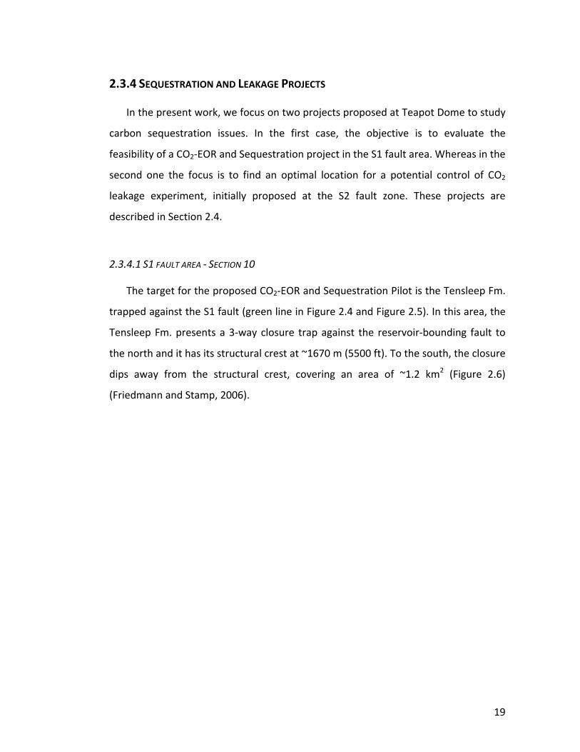
2.3.4.2 S2 FAULT AREA
The S2 fault area (orange lines in Figure 2.4) is structurally more complex than S1
area in Section 10. At the depth of the Tensleep Fm. there is not a distinct main fault,
but rather a set of faults with a different azimuths ranging from approximately 36° Az
(similar to the S1 fault) to 95° A; but the general trend is closer to the E‐W direction.
Figure 2.7 shows a time structure map of the 2nd Wall Creek member of the
Frontier Fm., and the S2 fault area. As it can be seen in the figure, the S2 fault
network presents a great complexity in geometry and azimuths, which was the first
reason to pre‐select this area as a candidate for the mentioned controlled leakage
21
experiment. Secondly, S2 fault zone outcrops support alkali springs and contains
hydrocarbon samples within fault veins and gouge, suggesting at some point the
occurrence of leakage through this network (Friedmann, et al, 2004).
Figure 2.7: Time structure map of the 2nd Wall Creek member showing the the S2 fault network (modified from McCutcheon, 2003). See location in Figure 2.5.
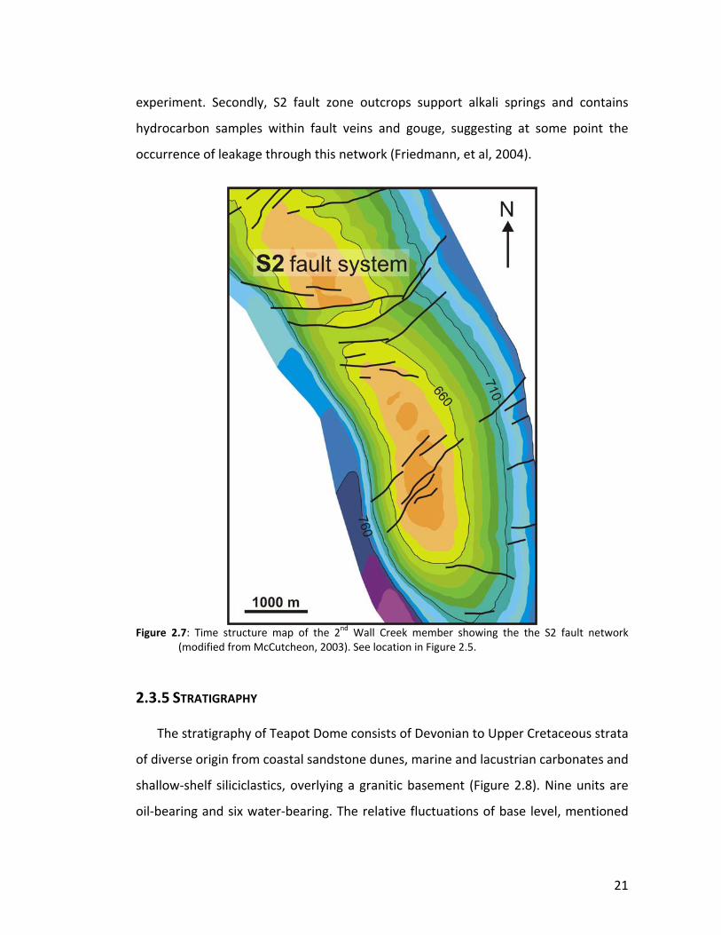
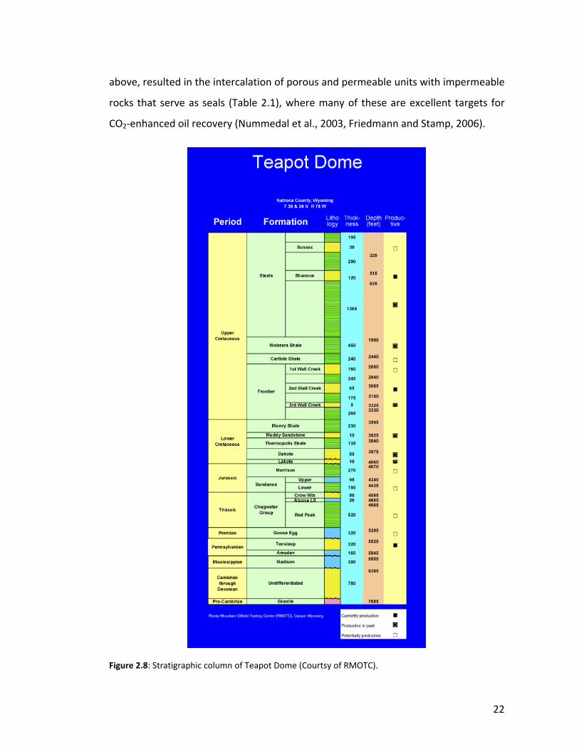
2.3.5 STRATIGRAPHY
The stratigraphy of Teapot Dome consists of Devonian to Upper Cretaceous strata
of diverse origin from coastal sandstone dunes, marine and lacustrian carbonates and
shallow‐shelf siliciclastics, overlying a granitic basement (Figure 2.8). Nine units are
oil‐bearing and six water‐bearing. The relative fluctuations of base level, mentioned
22
above, resulted in the intercalation of porous and permeable units with impermeable
rocks that serve as seals (Table 2.1), where many of these are excellent targets for
CO2‐enhanced oil recovery (Nummedal et al., 2003, Friedmann and Stamp, 2006).
Figure 2.8: Stratigraphic column of Teapot Dome (Courtsy of RMOTC).

23
Table 2.1: Main oil‐bearing and water‐bearing reservoir targets (Friedmann & Stamp, 2006).
24
The three traditional main reservoirs regarding cumulative production are the
Shannon Sandstone, member of the Steele Shale Fm., the Fractured Steele Shale and
the Second Wall Creek member of the Frontier Fm. All of them are of Upper
Cretaceous age. The Lower Cretaceous Dakota and Lakota Fms. and the Jurassic
Morrison Fm. are considered prospects for new discoveries. Whereas the
Pennsylvanian Tensleep Fm. is the deepest producing interval, and although it has a
relatively small cumulative production, Tensleep wells have had the highest IPs (i.e.
820 BOPD) since its exploitation began in mid‐70s (Milliken & Koespel, 2002).
2.3.5.1 TENSLEEP FORMATION
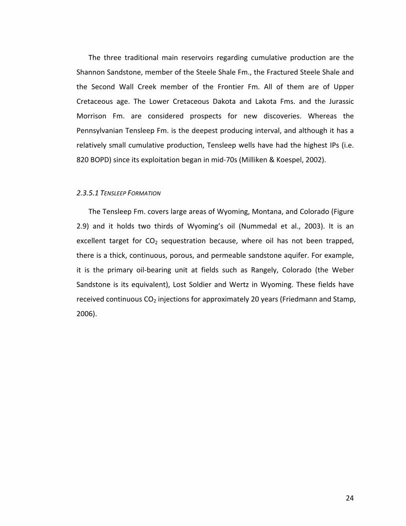
The Tensleep Fm. covers large areas of Wyoming, Montana, and Colorado (Figure
2.9) and it holds two thirds of Wyoming’s oil (Nummedal et al., 2003). It is an
excellent target for CO2 sequestration because, where oil has not been trapped,
there is a thick, continuous, porous, and permeable sandstone aquifer. For example,
it is the primary oil‐bearing unit at fields such as Rangely, Colorado (the Weber
Sandstone is its equivalent), Lost Soldier and Wertz in Wyoming. These fields have
received continuous CO2 injections for approximately 20 years (Friedmann and Stamp,
2006).
25
Figure 2.9: Paleogeographic map of Early Permian Tensleep extent; dark area represents area of thickest deposition (modified from Miller et al., 1992, Friedmann & Stamp, 2006).
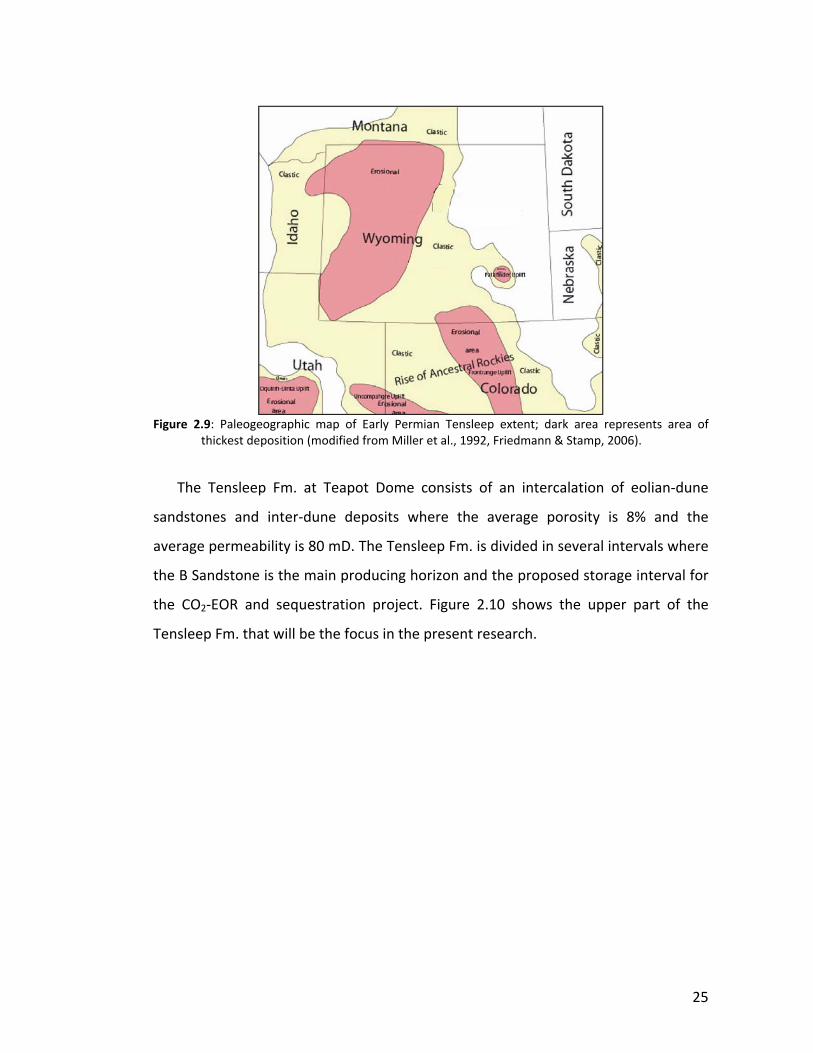
The Tensleep Fm. at Teapot Dome consists of an intercalation of eolian‐dune
sandstones and inter‐dune deposits where the average porosity is 8% and the
average permeability is 80 mD. The Tensleep Fm. is divided in several intervals where
the B Sandstone is the main producing horizon and the proposed storage interval for
the CO2‐EOR and sequestration project. Figure 2.10 shows the upper part of the
Tensleep Fm. that will be the focus in the present research.
26
Figure 2.10: Schematic stratigraphic column of reservoir (Tensleep Fm.) and caprock (Goose Egg Fm.). SS = sandstone, DS = dolostone.
The dune sandstones are permeable and porous intervals with different levels of
cementation, which affects their porosity, permeability and fracture intensity. The
inter‐dune deposits consist of thin sabkha carbonates, minor evaporates (mostly
anhydrite), and thin but widespread extensive beds of very low‐permeability
dolomicrites (Zhang et al., 2005).
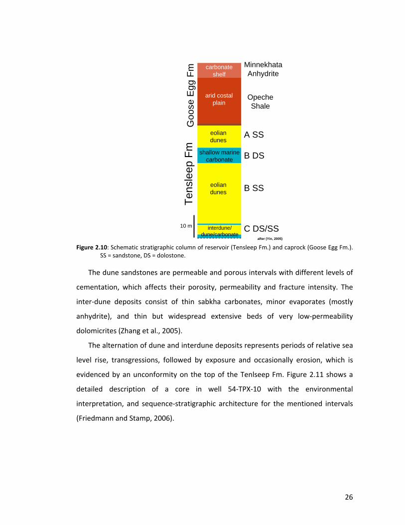
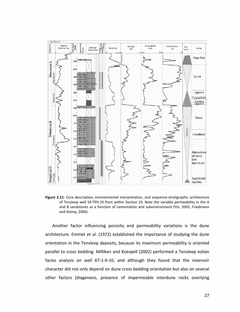
The alternation of dune and interdune deposits represents periods of relative sea
level rise, transgressions, followed by exposure and occasionally erosion, which is
evidenced by an unconformity on the top of the Tenlseep Fm. Figure 2.11 shows a
detailed description of a core in well 54‐TPX‐10 with the environmental
interpretation, and sequence‐stratigraphic architecture for the mentioned intervals
(Friedmann and Stamp, 2006).
Tens
leep
FmG
oose
Egg
Fm Minnekhata
Anhydrite
OpecheShale
A SS
B SS
C DS/SS
B DS
after (Yin, 2005)
carbonateshelf
arid costalplain
eoliandunes
shallow marinecarbonate
eoliandunes
interdune/dune/carbonate
10 m
27
Figure 2.11: Core description, environmental interpretation, and sequence‐stratigraphic architecture of Tensleep well 54‐TPX‐10 from within Section 10. Note the variable permeability in the A and B sandstones as a function of cementation and subenvironment (Yin, 2005; Friedmann and Stamp, 2006).
Another factor influencing porosity and permeability variations is the dune
architecture. Emmet et al. (1972) established the importance of studying the dune
orientation in the Tensleep deposits, because its maximum permeability is oriented
parallel to cross bedding. Milliken and Koespell (2002) performed a Tensleep eolian
facies analysis on well 67‐1‐X‐10, and although they found that the reservoir
character did not only depend on dune cross bedding orientation but also on several
other factors (diagenesis, presence of impermeable interdune rocks overlying
28
permeable dune sands, and fracturing) it will still be important, during a reservoir
characterization stage, to consider porosity and permeability anisotropy due to dune
orientation.
2.3.5.2 SEAL
The Permian Phosphoria Fm., locally denominated the Goose Egg Shale, is the
regional seal of the Tensleep Fm. throughout Wyoming. At Teapot Dome, consists of
more than 90 m (~300 ft) of shale, carbonate, and anhydrite (Minnekahta Member)
that has trapped more than 35 million bbl (5.6 million m3) of oil and dissolved natural
gas, demonstrating its effectiveness. In particular, in the S1 fault area, the depth of
these intervals ranges from ~1600 to ~1750 m below the surface.
A detailed characterization of a 48‐X‐28 well core, the only Teapot Dome well
where the cap‐rock has been cored, showed the structure of this interval as
consisting of a very tight cemented paleosoil interval overlying a weathering surface
on top of the Tensleep Fm (due to the mentioned unconformity) followed by the
Opeche Shale member, and the anhydrite on top of it (M. Milliken, personal
communication 2006).
2.3.6 FRACTURES
The key producing reservoirs at Teapot Dome, and much of the Rocky Mountains,
are fractured. In particular, at Teapot Dome, several of the producing zones are in
fractured shales, including the Niobrara and Steele shales (Figure 2.8).
Several authors (Lorenz and Cooper, 2004; Schwartz et al., 2005; Lorenz, 2007)
have described fractures in the Tensleep Fm., from cores, FMI logs and outcrops. All
of them coincide in that most of the fractures are vertical to near vertical. In
particular, at Teapot Dome, Lorenz and Cooper (2004) performed a fracture
characterization in core samples where they found an average of 1 fracture every 5 ft,
29
although with increasing cement content, they noted an increase in fracturing. In
high porosity sandstones, they described fracture intensity of approximately 1
fracture every 10 ft.; in dolomitic sandstones, 1 fracture every 3 ft.; and in heavily
cemented sandstones 1 fracture per ft.
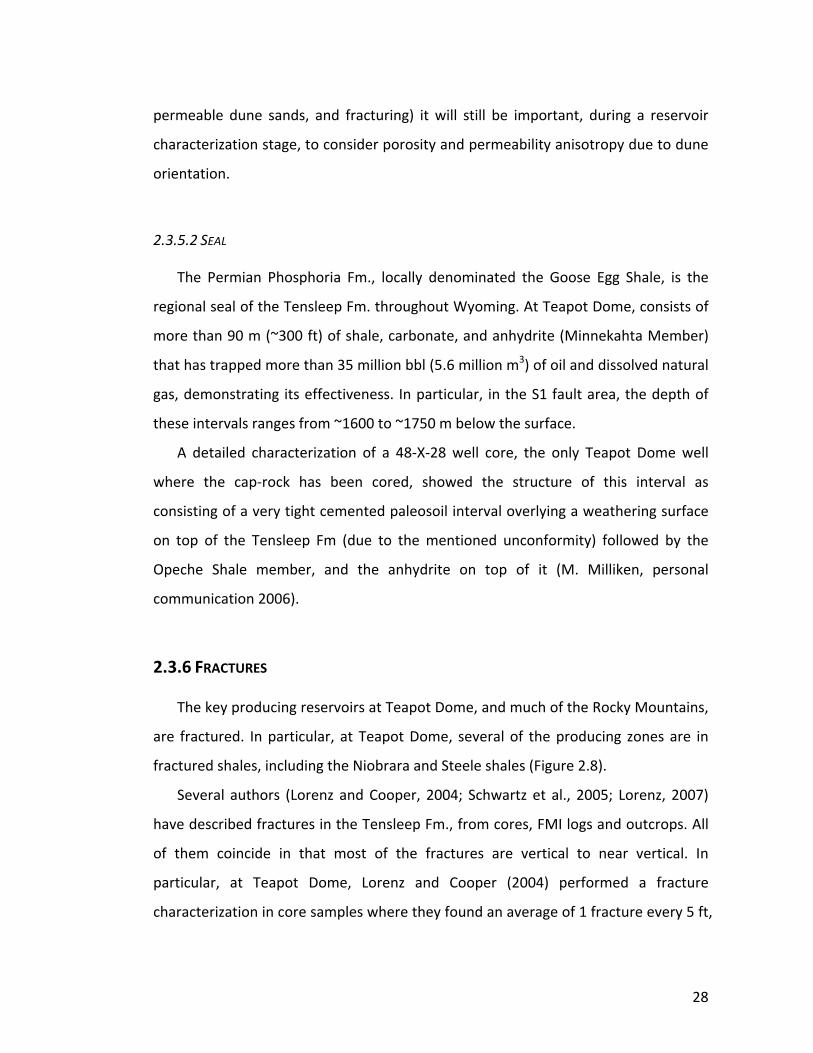
Schwartz et al. (2005) analyzed FMI logs of five wells located approximately
parallel to the axis of the anticline and found two main sets of open fractures, where
the dominant set has a mean Az = 100° and the secondary one a mean Az = 68°.
Figure 2.12: Fractures in the Tensleep Fm. from wells 25‐1‐X‐14, 61‐2‐X‐15, 67‐1‐X‐10 and 48‐X‐28 (left); fractrures in the caprock from wells 25‐1‐X‐14, 67‐1‐X‐10 and 48‐X‐28 (right). See Figure 2.5 for well location.
Figure 2.12 shows the fractures we mapped in the Tensleep Fm. and in the
caprock from 4 FMI logs in the area. The role of these fractures will be discussed in
the further chapters.
2.4 TEAPOT DOME CARBON STORAGE TEST CENTER
Teapot Dome Field Experimental Facility presents an exciting opportunity to
conduct CO2 sequestration experiments for several reasons. As mentioned before,
30
the site is fully owned by the US government and it is operated by the Rocky
Mountain Oilfield Testing Center (RMOTC). This Federal ownership provides several
significant advantages. It provides a stable platform for long‐term scientific
investigations in a steady business context without the commercial drivers of a
privately owned oil field. In addition, the field has a high density of wells, and the
extensive data set from Teapot Dome and all experimental results are in the public
domain (Friedmann et al., 2004b).
Field infrastructure includes roads, pipelines, water lines, water‐treatment
facilities, a gas‐processing plant, workover rig, etc. Currently, RMOTC owns and
operates 1 drilling rig and 600 pump jacks of varying sizes. Drilling costs for certain
work are covered by RMOTC, and an internal committee of scientists and engineers
approves drilling programs in coordination with all other efforts (e.g., the current site
characterization and CO2 program).
2.4.1 DATA SET
The field covers nearly 10,000 ac (40.5 km2) and contains more than 2200 wells
total, of which more than 1200 may be accessed (Table 2.2). Of these, about 600 are
currently producing, and more than 400 penetrate to a depth greater than 2700 ft
(823 m). All cores, well logs, mud logs, completion descriptions, and production data
from these wells are in the public domain (RMOTC, 2005a, b, c).
31
Table 2.2: Data types and format at Teapot Dome (Friedmann and Stamp, 2006).
2.4.1.1 SEISMIC
The 3D seismic cube is a post‐stack migrated filtered volume (also unfiltered is
available). Five horizons have been interpreted (McCutcheon, 2003), as well as the
main faults associated with them. The interpreted reflectors are the Second Wall
Creek Sandstone, Lakota Sandstone (a good quality reflector that provides mid‐level
structural control across Teapot Dome), Red Peak Member of Chugwater Fm. (also a
good quality reflector), the Tensleep Fm. and the Precambrian basement. Major fault
cuts were mapped only in the intersection with the seismic horizons, but systematic
correlation of each fault has not been done.
2.4.1.2 WELL LOGS
Of the 1300 wells at Teapot Dome, around 43 have penetrated the Tensleep Fm.,
and most of them are in the denominated Section 10 (Figure 2.13). In table 2.3, we
summarize the wells in the study area that present the most complete set of logs,
including FMI, cores, as well as the sonic logs and drilling reports.
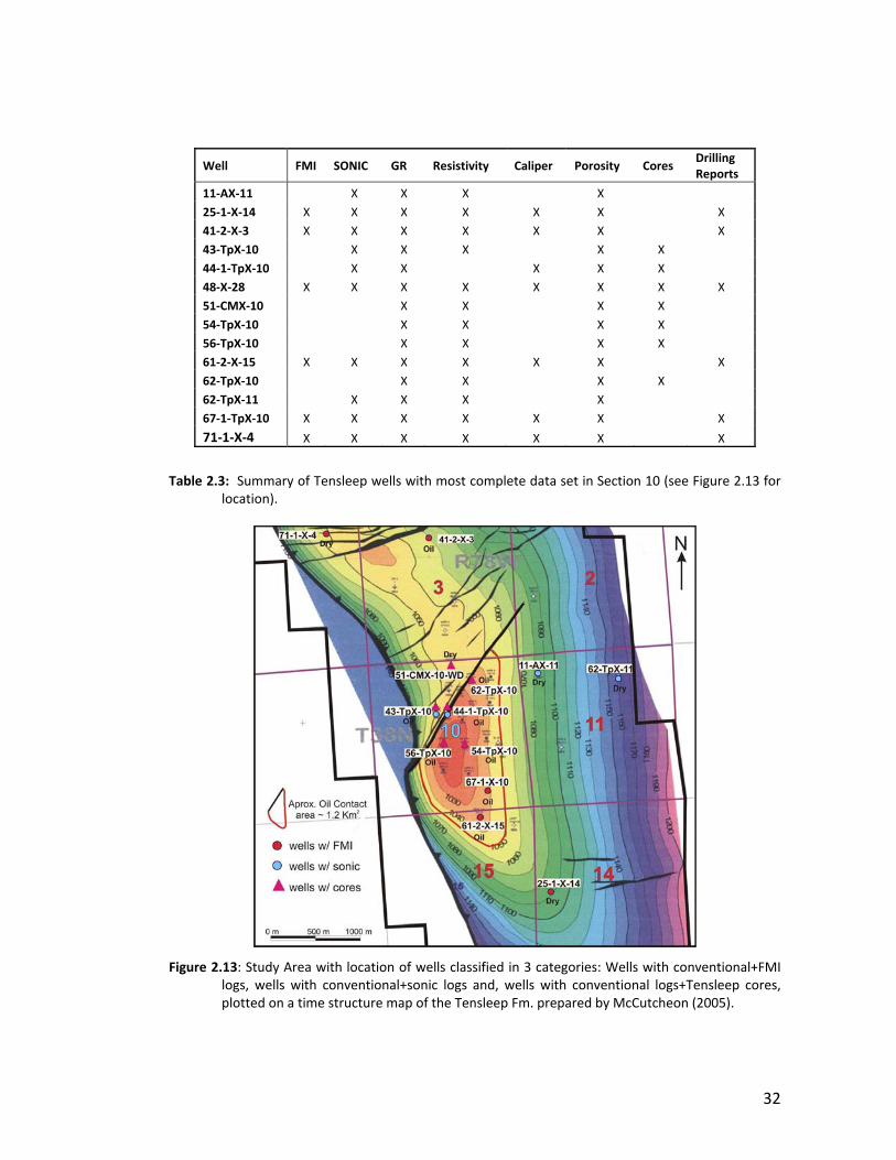
32
Well FMI SONIC GR Resistivity Caliper Porosity Cores Drilling Reports
11‐AX‐11 X X X X 25‐1‐X‐14 X X X X X X X 41‐2‐X‐3 X X X X X X X 43‐TpX‐10 X X X X X 44‐1‐TpX‐10 X X X X X 48‐X‐28 X X X X X X X X 51‐CMX‐10 X X X X 54‐TpX‐10 X X X X 56‐TpX‐10 X X X X 61‐2‐X‐15 X X X X X X X 62‐TpX‐10 X X X X 62‐TpX‐11 X X X X 67‐1‐TpX‐10 X X X X X X X
71‐1‐X‐4 X X X X X X X
Table 2.3: Summary of Tensleep wells with most complete data set in Section 10 (see Figure 2.13 for location).
Figure 2.13: Study Area with location of wells classified in 3 categories: Wells with conventional+FMI
logs, wells with conventional+sonic logs and, wells with conventional logs+Tensleep cores, plotted on a time structure map of the Tensleep Fm. prepared by McCutcheon (2005).
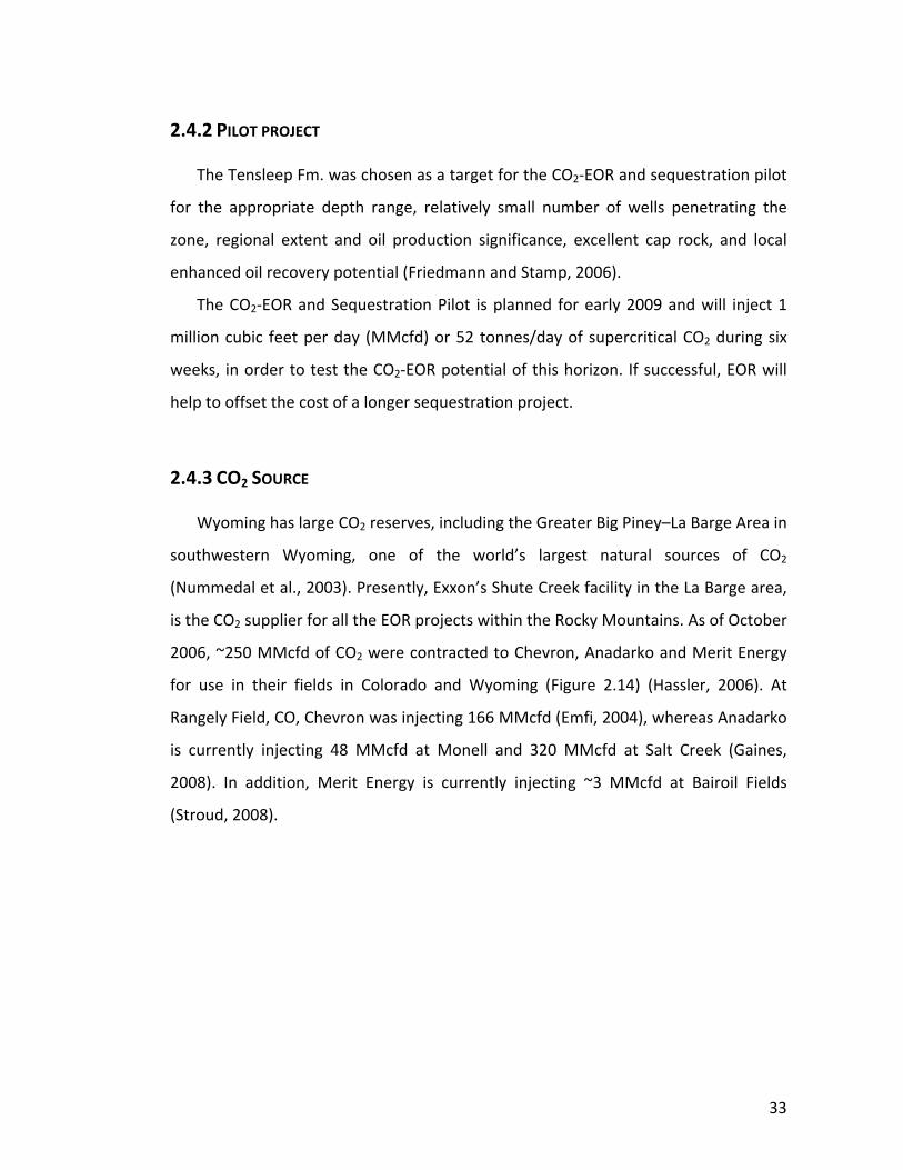
33
2.4.2 PILOT PROJECT
The Tensleep Fm. was chosen as a target for the CO2‐EOR and sequestration pilot
for the appropriate depth range, relatively small number of wells penetrating the
zone, regional extent and oil production significance, excellent cap rock, and local
enhanced oil recovery potential (Friedmann and Stamp, 2006).
The CO2‐EOR and Sequestration Pilot is planned for early 2009 and will inject 1
million cubic feet per day (MMcfd) or 52 tonnes/day of supercritical CO2 during six
weeks, in order to test the CO2‐EOR potential of this horizon. If successful, EOR will
help to offset the cost of a longer sequestration project.
2.4.3 CO2 SOURCE
Wyoming has large CO2 reserves, including the Greater Big Piney–La Barge Area in
southwestern Wyoming, one of the world’s largest natural sources of CO2
(Nummedal et al., 2003). Presently, Exxon’s Shute Creek facility in the La Barge area,
is the CO2 supplier for all the EOR projects within the Rocky Mountains. As of October
2006, ~250 MMcfd of CO2 were contracted to Chevron, Anadarko and Merit Energy
for use in their fields in Colorado and Wyoming (Figure 2.14) (Hassler, 2006). At
Rangely Field, CO, Chevron was injecting 166 MMcfd (Emfi, 2004), whereas Anadarko
is currently injecting 48 MMcfd at Monell and 320 MMcfd at Salt Creek (Gaines,
2008). In addition, Merit Energy is currently injecting ~3 MMcfd at Bairoil Fields
(Stroud, 2008).
34
Figure 2.14: Existing carbon dioxide infrastructure in the region. Primary infrastructure for CO2 delivery is owned by Exxon, Chevron and Anadarko (or their affiliates). Exxon: from Shute Creek through Rock Springs and on to Bairoil. Chevron: from Rock Springs to Rangely. Anadarko: from Bairoil to Salt Creek (Hassler, 2006).
Exxon Mobil’s Shute Creek gas processing facility was built in 1986 and produces
CO2 in association with sour natural gas from southwest Wyoming. The plant, that
also produces methane, is the largest sulfur‐producer in Wyoming and the largest
helium producer in the United States (WSGS Carbon Dioxide Group). An average of
207 MMcfd of CO2 was sold in 2007 for enhanced oil recovery, but another 181
MMcfd were vented (Bleizeffer, 2008). This corresponds to a total of 7.33x10⁶
tonnes/yr CO2 separated at Shute Creek.
The Teapot Dome Tensleep pilot will take advantage of the pipeline already
constructed from Shute Creek facility to Anadarko’s Salt Creek for the Second Wall
Creek EOR project. The pipeline supplies Salt Creek with anthropogenic CO2, and
since the possibility of constructing a pipeline extension from Salt Creek into Teapot
35
Dome is not clear yet; CO2 is expected to be delivered by truck for the start of the
pilot (Friedmann and Stamp, 2006).
2.5 SUMMARY
In this chapter, we presented an overview of Teapot Dome’s geology, as well as
the characteristics of the National Carbon Storage Test Center and the proposed
experiments, which are the focus of this dissertation. Most of the work that will be
presented in the following chapters is related to the CO2‐EOR and sequestration pilot,
planned in the Section 10 area, where the Tensleep Fm. is trapped against the S1
fault.
36
CHAPTER 3
SEAL INTEGRITY AND FEASIBILITY OF
CO2 SEQUESTRATION IN THE TEAPOT
DOME EOR PILOT: GEOMECHANICAL
SITE CHARACTERIZATION
3.1 ABSTRACT
This paper reports on a preliminary investigation of CO2 sequestration and seal
integrity at Teapot Dome oil field, Wyoming, USA, with the objective of predicting the
potential risk of CO2 leakage along reservoir‐bounding faults. CO2 injection into
reservoirs creates anomalously high pore pressure at the top of the reservoir that
could potentially hydraulically fracture the caprock or trigger slip on reservoir‐
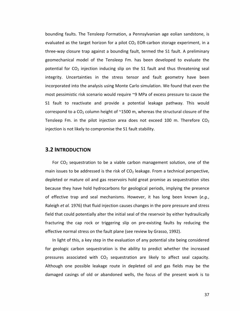
37
bounding faults. The Tensleep Formation, a Pennsylvanian age eolian sandstone, is
evaluated as the target horizon for a pilot CO2 EOR‐carbon storage experiment, in a
three‐way closure trap against a bounding fault, termed the S1 fault. A preliminary
geomechanical model of the Tensleep Fm. has been developed to evaluate the
potential for CO2 injection inducing slip on the S1 fault and thus threatening seal
integrity. Uncertainties in the stress tensor and fault geometry have been
incorporated into the analysis using Monte Carlo simulation. We found that even the
most pessimistic risk scenario would require ~9 MPa of excess pressure to cause the
S1 fault to reactivate and provide a potential leakage pathway. This would
correspond to a CO2 column height of ~1500 m, whereas the structural closure of the
Tensleep Fm. in the pilot injection area does not exceed 100 m. Therefore CO2
injection is not likely to compromise the S1 fault stability.
3.2 INTRODUCTION
For CO2 sequestration to be a viable carbon management solution, one of the
main issues to be addressed is the risk of CO2 leakage. From a technical perspective,
depleted or mature oil and gas reservoirs hold great promise as sequestration sites
because they have hold hydrocarbons for geological periods, implying the presence
of effective trap and seal mechanisms. However, it has long been known (e.g.,
Raleigh et al. 1976) that fluid injection causes changes in the pore pressure and stress
field that could potentially alter the initial seal of the reservoir by either hydraulically
fracturing the cap rock or triggering slip on pre‐existing faults by reducing the
effective normal stress on the fault plane (see review by Grasso, 1992).
In light of this, a key step in the evaluation of any potential site being considered
for geologic carbon sequestration is the ability to predict whether the increased
pressures associated with CO2 sequestration are likely to affect seal capacity.
Although one possible leakage route in depleted oil and gas fields may be the
damaged casings of old or abandoned wells, the focus of the present work is to

38
evaluate the potential risk of CO2 leakage through natural pathways by inducing slip
on faults that are currently sealing and bounding the hydrocarbon reservoirs. It is
thus essential to study the relationship between faults and the present‐day stress
field to predict which faults could be potential leakage routes.
Another way of compromising seal integrity is by hydrofracturing the cap rock,
which occurs when the pore pressure at the top of the reservoir is as high as the least
principal stress in the overlying unit. In both cases, geomechanical characterization
can be used to derive the pressures and rates of injection needed to reach those
critical values and can therefore help evaluate the potential risk of leakage.
3.3 TEAPOT DOME CO2 EOR‐CARBON STORAGE PILOT
The Teapot Dome Field Experimental Facility (Figure 3.1) is owned by the U.S.
government and operated by the U.S. Department of Energy (DOE) and the Rocky
Mountain Oilfield Testing Center (RMOTC). This federal ownership assures a platform
for long‐term scientific investigations in a stable business context. The extensive data
set of Teapot Dome is in the public domain, thus facilitating research of all kinds.
These unique characteristics make Teapot Dome an ideal laboratory to conduct an
EOR ‐ Carbon Storage experiment in a mature oil reservoir. To evaluate the scientific
and technical feasibility, the project team is working with interested industry and
research partners to design the first CO2 injection experiment, a small, short‐duration
EOR pilot, using existing wells and infrastructure. Project execution will be primarily
contingent upon receiving adequate support from RMOTC’s industry and research
partners. The project envisioned would target the Tensleep Formation, with a
minimum of ~60 tons/day CO2 for a minimum of ~1.5 months.
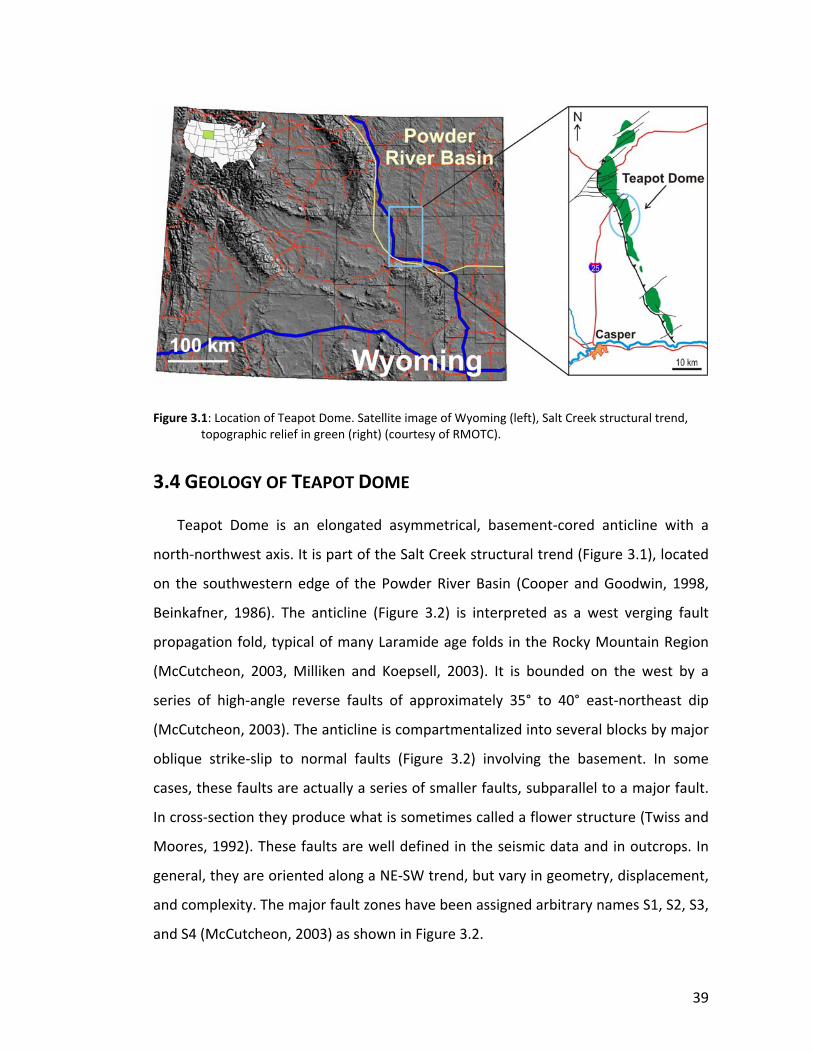
39
Figure 3.1: Location of Teapot Dome. Satellite image of Wyoming (left), Salt Creek structural trend, topographic relief in green (right) (courtesy of RMOTC).
3.4 GEOLOGY OF TEAPOT DOME
Teapot Dome is an elongated asymmetrical, basement‐cored anticline with a
north‐northwest axis. It is part of the Salt Creek structural trend (Figure 3.1), located
on the southwestern edge of the Powder River Basin (Cooper and Goodwin, 1998,
Beinkafner, 1986). The anticline (Figure 3.2) is interpreted as a west verging fault
propagation fold, typical of many Laramide age folds in the Rocky Mountain Region
(McCutcheon, 2003, Milliken and Koepsell, 2003). It is bounded on the west by a
series of high‐angle reverse faults of approximately 35° to 40° east‐northeast dip
(McCutcheon, 2003). The anticline is compartmentalized into several blocks by major
oblique strike‐slip to normal faults (Figure 3.2) involving the basement. In some
cases, these faults are actually a series of smaller faults, subparallel to a major fault.
In cross‐section they produce what is sometimes called a flower structure (Twiss and
Moores, 1992). These faults are well defined in the seismic data and in outcrops. In
general, they are oriented along a NE‐SW trend, but vary in geometry, displacement,
and complexity. The major fault zones have been assigned arbitrary names S1, S2, S3,
and S4 (McCutcheon, 2003) as shown in Figure 3.2.
40
Figure 3.2: NW‐SE cross section through Teapot Dome (left). Depth‐structure map of 2nd Wall Creek Sandstone with locations of seismic line (right) (Friedmann et al., 2004).
The stratigraphy of Teapot Dome consists of Upper Cretaceous to Mississippian
strata of diverse origin ranging from offshore sediments to coastal sandstone dunes
over a granitic basement. The Tensleep Formation, of Pennsylvanian age, is the
deepest hydrocarbon producing interval in the anticline. It contains multiple
sequence boundaries in response to frequent and high‐amplitude sea level changes
(Zhang et al., 2005). In this area it consists of interdune deposits such as eolian
sandstones, sabkha carbonates, evaporites (mostly anhydrite), and extensive beds of
very low permeability dolomicrites. The average porosity is 10% (5 – 20% range), and
the average permeability is 30 mD (10 – 100 mD range). The average net thickness is
15 m. The reservoir has a strong aquifer drive and therefore hydrostatic reservoir
pressure, and the reservoir temperature is ~88°C. The Tensleep Formation is divided
into several intervals, of which the approximately 30 m thick B‐Sandstone is the main
producing horizon and the proposed storage interval for this experiment.
The Opeche Shale plus the anhydrite of the Minnekahta Member of the Permian
Goose Egg Formation (Figure 3.4) comprise the regional seal of the Tensleep Fm.
throughout Wyoming. At the top of the Tensleep Fm. there is a tightly cemented
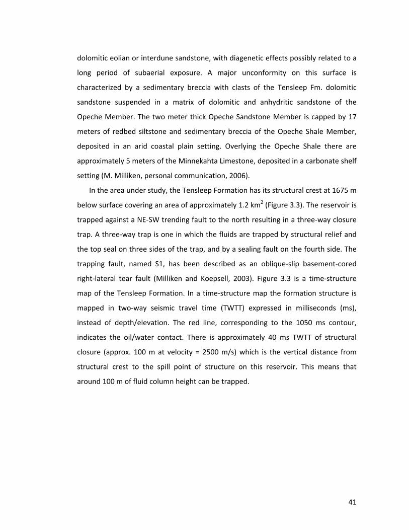
41
dolomitic eolian or interdune sandstone, with diagenetic effects possibly related to a
long period of subaerial exposure. A major unconformity on this surface is
characterized by a sedimentary breccia with clasts of the Tensleep Fm. dolomitic
sandstone suspended in a matrix of dolomitic and anhydritic sandstone of the
Opeche Member. The two meter thick Opeche Sandstone Member is capped by 17
meters of redbed siltstone and sedimentary breccia of the Opeche Shale Member,
deposited in an arid coastal plain setting. Overlying the Opeche Shale there are
approximately 5 meters of the Minnekahta Limestone, deposited in a carbonate shelf
setting (M. Milliken, personal communication, 2006).
In the area under study, the Tensleep Formation has its structural crest at 1675 m
below surface covering an area of approximately 1.2 km2 (Figure 3.3). The reservoir is
trapped against a NE‐SW trending fault to the north resulting in a three‐way closure
trap. A three‐way trap is one in which the fluids are trapped by structural relief and
the top seal on three sides of the trap, and by a sealing fault on the fourth side. The
trapping fault, named S1, has been described as an oblique‐slip basement‐cored
right‐lateral tear fault (Milliken and Koepsell, 2003). Figure 3.3 is a time‐structure
map of the Tensleep Formation. In a time‐structure map the formation structure is
mapped in two‐way seismic travel time (TWTT) expressed in milliseconds (ms),
instead of depth/elevation. The red line, corresponding to the 1050 ms contour,
indicates the oil/water contact. There is approximately 40 ms TWTT of structural
closure (approx. 100 m at velocity = 2500 m/s) which is the vertical distance from
structural crest to the spill point of structure on this reservoir. This means that
around 100 m of fluid column height can be trapped.
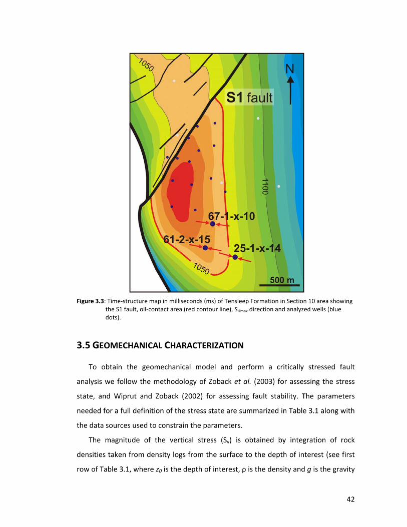
42
Figure 3.3: Time‐structure map in milliseconds (ms) of Tensleep Formation in Section 10 area showing the S1 fault, oil‐contact area (red contour line), SHmax direction and analyzed wells (blue dots).
3.5 GEOMECHANICAL CHARACTERIZATION
To obtain the geomechanical model and perform a critically stressed fault
analysis we follow the methodology of Zoback et al. (2003) for assessing the stress
state, and Wiprut and Zoback (2002) for assessing fault stability. The parameters
needed for a full definition of the stress state are summarized in Table 3.1 along with
the data sources used to constrain the parameters.
The magnitude of the vertical stress (Sv) is obtained by integration of rock
densities taken from density logs from the surface to the depth of interest (see first
row of Table 3.1, where z0 is the depth of interest, ρ is the density and g is the gravity
43
acceleration). Density logs measure the bulk density of the rocks in the wellbore
walls through gamma ray emissions. The proportion of gamma rays emitted by the
source and back‐scattered to the detector depends on the electron density of the
formation and therefore its matrix density (Jahn et al., 1998).
The least principal stress, S3, which is usually the minimum horizontal principal
stress (Shmin), can be obtained from the analysis of hydraulic fracturing via either
minifracs or extended leak‐off tests after the casing is set. Hydraulic fractures allow
the determination of S3 orientation and magnitude since they always propagate
perpendicular to the least principal stress in the earth (Hubbert and Willis, 1957).
While Sv and S3 are relatively straightforward to estimate, the maximum
horizontal stress (SHmax) magnitude can be obtained in different ways by modelling
wellbore failure features such as drilling‐induced tensile fractures (if Sv, Shmin and
pore pressure (Pp) values are known) or stress‐induced wellbore breakouts (if Sv,
Shmin, Pp and the rock strength are known). The orientation of the horizontal principal
stresses in vertical wells can be straightforwardly determined from wellbore failure
orientations. Drilling‐induced tensile fractures propagate parallel to SHmax, whereas
breakouts form at the azimuth of Shmin. Under normal drilling conditions, the
occurrence of drilling‐induced tensile fractures in a vertical well usually indicates a
strike‐slip faulting stress state (Zoback et al., 2003).
44
Parameter Data
Vertical Stress (Sv) Density logs: ( ) ∫=0
00
z
v gdzzS ρ
Minimum horizontal Stress (Shmin)
LOT, XLOT, minifrac
Maximum horizontal Stress (SHmax)
Modeling wellbore failures
Stress orientation Orientation of wellbore failures
Pore Pressure Measure, sonic logs
Rock strength Lab, logs, modeling well failure
Faults and fractures Seismic, wellbore imaging
Table 3.1: Parameters and data needed to define the stress tensor and the geomechanical model.
Density, sonic and Formation Microresistivity Imager (FMI) logs in the 67‐1‐x‐10,
61‐2‐x‐15 and 25‐1‐x‐14 wells (see Figure 3.3 for well locations) were analyzed to
quantify the stress tensor (Sv, SHmax and Shmin) in the area of interest. A sonic log
measures the speed of sound in the wall of the borehole, and is related to both the
porosity and lithology of the rock being measured, whereas the FMI log makes a
detailed image of the rocks on all sides of the well hole by measuring resisitivity of
the rock.
Stress Orientation from FMI logs
Drilling‐induced tensile fractures were analyzed in FMI logs from the three study
wells. Interactive image analysis yielded 420 observations of drilling‐induced tensile
fractures over a depth range of 400 – 1800 m (Figure 3.4). The average maximum
horizontal stress (SHmax) direction is 116° ±15° AZ (N64°W). This value is consistent
with the SHmax orientation of 105° AZ (N75°W), observed by Milliken and Koepsell
(2003) in well 67‐1‐x‐10. If we consider only the drilling‐induced tensile fractures in
the Tensleep Fm., the direction of SHmax is 100° ±15° AZ (N80°W).
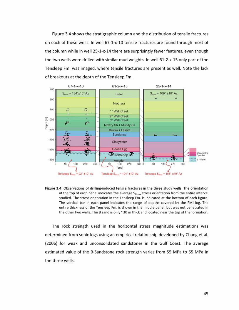
45
Figure 3.4 shows the stratigraphic column and the distribution of tensile fractures
on each of these wells. In well 67‐1‐x‐10 tensile fractures are found through most of
the column while in well 25‐1‐x‐14 there are surprisingly fewer features, even though
the two wells were drilled with similar mud weights. In well 61‐2‐x‐15 only part of the
Tensleep Fm. was imaged, where tensile fractures are present as well. Note the lack
of breakouts at the depth of the Tensleep Fm.
Figure 3.4: Observations of drilling‐induced tensile fractures in the three study wells. The orientation at the top of each panel indicates the average SHmax stress orientation from the entire interval studied. The stress orientation in the Tensleep Fm. is indicated at the bottom of each figure. The vertical bar in each panel indicates the range of depths covered by the FMI log. The entire thickness of the Tensleep Fm. is shown in the middle panel, but was not penetrated in the other two wells. The B sand is only ~30 m thick and located near the top of the formation.
The rock strength used in the horizontal stress magnitude estimations was
determined from sonic logs using an empirical relationship developed by Chang et al.
(2006) for weak and unconsolidated sandstones in the Gulf Coast. The average
estimated value of the B‐Sandstone rock strength varies from 55 MPa to 65 MPa in
the three wells.
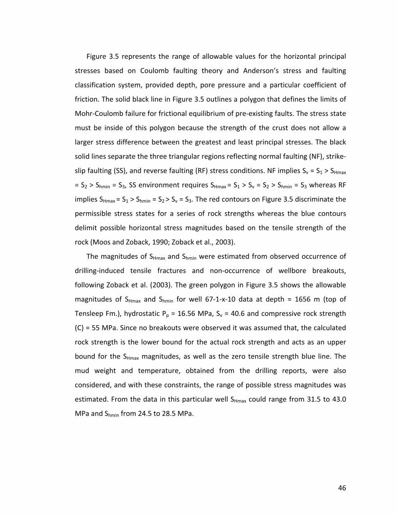
46
Figure 3.5 represents the range of allowable values for the horizontal principal
stresses based on Coulomb faulting theory and Anderson’s stress and faulting
classification system, provided depth, pore pressure and a particular coefficient of
friction. The solid black line in Figure 3.5 outlines a polygon that defines the limits of
Mohr‐Coulomb failure for frictional equilibrium of pre‐existing faults. The stress state
must be inside of this polygon because the strength of the crust does not allow a
larger stress difference between the greatest and least principal stresses. The black
solid lines separate the three triangular regions reflecting normal faulting (NF), strike‐
slip faulting (SS), and reverse faulting (RF) stress conditions. NF implies Sv = S1 > SHmax
= S2 > Shmin = S3, SS environment requires SHmax = S1 > Sv = S2 > Shmin = S3 whereas RF
implies SHmax = S1 > Shmin = S2 > Sv = S3. The red contours on Figure 3.5 discriminate the
permissible stress states for a series of rock strengths whereas the blue contours
delimit possible horizontal stress magnitudes based on the tensile strength of the
rock (Moos and Zoback, 1990; Zoback et al., 2003).
The magnitudes of SHmax and Shmin were estimated from observed occurrence of
drilling‐induced tensile fractures and non‐occurrence of wellbore breakouts,
following Zoback et al. (2003). The green polygon in Figure 3.5 shows the allowable
magnitudes of SHmax and Shmin for well 67‐1‐x‐10 data at depth = 1656 m (top of
Tensleep Fm.), hydrostatic Pp = 16.56 MPa, Sv = 40.6 and compressive rock strength
(C) = 55 MPa. Since no breakouts were observed it was assumed that, the calculated
rock strength is the lower bound for the actual rock strength and acts as an upper
bound for the SHmax magnitudes, as well as the zero tensile strength blue line. The
mud weight and temperature, obtained from the drilling reports, were also
considered, and with these constraints, the range of possible stress magnitudes was
estimated. From the data in this particular well SHmax could range from 31.5 to 43.0
MPa and Shmin from 24.5 to 28.5 MPa.
47
Figure 3.5: Stress polygon for well 67‐1‐x‐10 (see explanation in text) at depth = 1656 m (top of Tensleep Fm.), Pp = 16.56 MPa, Sv = 40.6 and compressive rock strength = 55 MPa. Red lines are isovalues of rock strength and blue lines represents isovalues of tensile rock strength.
The analysis of the three studied wells yielded a NF/SS faulting stress state where
SHmax ≈ Sv > Shmin. This is supported by fault movement observed in the youngest
sections of the 3D seismic cube and by the displacements on NE/SW faults observed
in the surface outcrops and trenches (Milliken, 2005).
Due to the absence of leakoff or minifrac tests in the Tensleep Fm. to obtain the
magnitude of Shmin (which would also better constrain the magnitude of SHmax), the
critically stressed fault analysis was first performed with an Shmin gradient of 0.6Sv and
SHmax = Sv expected for a NF/SS environment. Available data from a minifrac test
performed in the 2nd Wall Creek reservoir confirms Shmin = 0.6Sv. This minifrac test
was performed in well 71‐1‐ax‐4, roughly 2 km northwest of the area under study,
48
where the 2nd Wall Creek reservoir is at approximately 900 m depth and 720 m above
the top of the Tensleep Fm.
With this information, a 2nd order stress tensor (S) that only varies with depth was
defined as the base case scenario to estimate the leakage potential of the S1 fault.
Since the present stress state corresponds to a NF/SS environment, S1 = SHmax, S2 = Sv
and S3 = Shmin (see Eq. 3.1).
⎥⎥⎥
⎦
⎤
⎢⎢⎢
⎣
⎡=
⎥⎥⎥
⎦
⎤
⎢⎢⎢
⎣
⎡=
⎥⎥⎥
⎦
⎤
⎢⎢⎢
⎣
⎡=
v
v
v
h
v
H
SS
S
SS
S
SS
SS
6.0000000
000000
000000
min
max
3
2
1
(3.1)
3.6 FAULT SLIP POTENTIAL USING COULOMB CRITERION
The S1 fault was mapped in the available 3D seismic survey and converted to
depth using the seismic dip processing moveout (DMO) velocities. To determine the
risk of leakage through the S1 fault, the authors evaluated the state of stress and
pore pressure acting on the fault plane following the methodology of Wiprut and
Zoback (2002) described below.
It is important to note that the orientation of the S1 fault has an azimuth of 36°,
which is nearly perpendicular to SHmax (see Figure 3.3). Therefore, it immediately
appears unlikely that this fault could slip in a NF/SS stress field.
To perform the quantitative analysis, the shear (τ) and normal stresses (Sn) were
calculated for each element of the fault. Then Coulomb failure criteria were applied
to predict the critical pressure (Pc) necessary to reactivate fault slip, assuming a
coefficient of friction (μ) of 0.6.
μτ /−= nc SP (3.2)
Comparing this Pc with a reference Pp, modeled from the pressure data of the
field, a critical pressure perturbation (Pcp) was obtained. Pcp indicates the pore
pressure change to enable a fault element to slip given the stress state, fault

49
orientation and reference Pp. In this analysis, it is assumed that active faults are
potential conduits for fluid migration such that Pcp indicates the leakage potential for
each portion of the fault (Figure 3.6a). It is worth noting that this is a conservative
approach for evaluating likelihood of CO2 leakage along the fault, even though the
amount of potential leakage could be quite small if the area of fault slip is small.
For the base case stress scenario defined in the previous section, at the depth of
the Tensleep Formation (red line in Figure 3.6a), approximately 16 MPa of excess
pressure would be required to cause the fault to slip. This corresponds to a CO2
column height of approximately 2300 m (at a density of 700 kg/m3). Since the
average closure of the Tensleep Formation in this area is no more than 100 m, it is
anticipated that the S1 fault is not at risk of reactivation and therefore will not be a
leakage pathway for CO2 migration.
Figure 3.6a: Fault surface color‐coded with critical pressure perturbation values indicating the fault slip potential. At the Tensleep Fm. (red line), ~16 MPa of excess pressure would be required to cause the fault to slip.
[m]
Dep
th [m
]
N
[m]
[MPa]
Critical Pp Pert
Tensleep Fm
[m]
Dep
th [m
]
N
[m]
[MPa]
Critical Pp Pert
Tensleep Fm
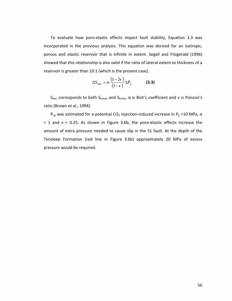
50
To evaluate how poro‐elastic effects impact fault stability, Equation 3.3 was
incorporated in the previous analysis. This equation was derived for an isotropic,
porous and elastic reservoir that is infinite in extent. Segall and Fitzgerald (1996)
showed that this relationship is also valid if the ratio of lateral extent to thickness of a
reservoir is greater than 10:1 (which is the present case).
( )( ) pHor PS Δ−−
=Δννα
121
(3.3)
SHor corresponds to both SHmax and Shmin, α is Biot’s coefficient and ν is Poisson’s
ratio (Brown et al., 1994).
Pcp was estimated for a potential CO2 injection‐induced increase in Pp =10 MPa, α
= 1 and ν = 0.25. As shown in Figure 3.6b, the poro‐elastic effects increase the
amount of extra pressure needed to cause slip in the S1 fault. At the depth of the
Tensleep Formation (red line in Figure 3.6b) approximately 20 MPa of excess
pressure would be required.
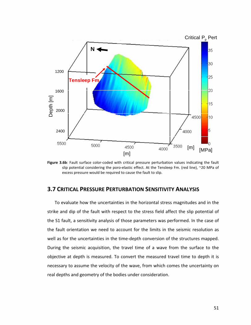
51
Figure 3.6b: Fault surface color‐coded with critical pressure perturbation values indicating the fault slip potential considering the poro‐elastic effect. At the Tensleep Fm. (red line), ~20 MPa of excess pressure would be required to cause the fault to slip.
3.7 CRITICAL PRESSURE PERTURBATION SENSITIVITY ANALYSIS
To evaluate how the uncertainties in the horizontal stress magnitudes and in the
strike and dip of the fault with respect to the stress field affect the slip potential of
the S1 fault, a sensitivity analysis of those parameters was performed. In the case of
the fault orientation we need to account for the limits in the seismic resolution as
well as for the uncertainties in the time‐depth conversion of the structures mapped.
During the seismic acquisition, the travel time of a wave from the surface to the
objective at depth is measured. To convert the measured travel time to depth it is
necessary to assume the velocity of the wave, from which comes the uncertainty on
real depths and geometry of the bodies under consideration.
[m]
Dep
th [m
]N
[m] [MPa]
Tensleep Fm
Critical Pp Pert
1200
1600
2000
2400
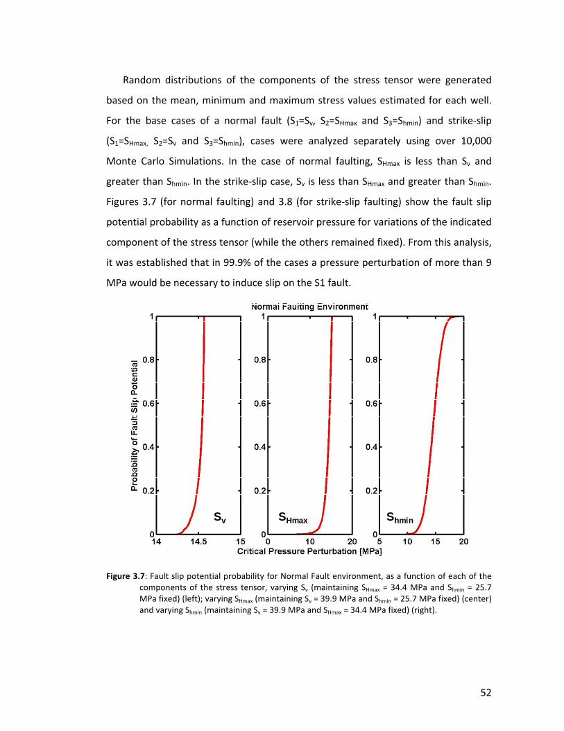
52
Random distributions of the components of the stress tensor were generated
based on the mean, minimum and maximum stress values estimated for each well.
For the base cases of a normal fault (S1=Sv, S2=SHmax and S3=Shmin) and strike‐slip
(S1=SHmax, S2=Sv and S3=Shmin), cases were analyzed separately using over 10,000
Monte Carlo Simulations. In the case of normal faulting, SHmax is less than Sv and
greater than Shmin. In the strike‐slip case, Sv is less than SHmax and greater than Shmin.
Figures 3.7 (for normal faulting) and 3.8 (for strike‐slip faulting) show the fault slip
potential probability as a function of reservoir pressure for variations of the indicated
component of the stress tensor (while the others remained fixed). From this analysis,
it was established that in 99.9% of the cases a pressure perturbation of more than 9
MPa would be necessary to induce slip on the S1 fault.
Figure 3.7: Fault slip potential probability for Normal Fault environment, as a function of each of the components of the stress tensor, varying Sv (maintaining SHmax = 34.4 MPa and Shmin = 25.7 MPa fixed) (left); varying SHmax (maintaining Sv = 39.9 MPa and Shmin = 25.7 MPa fixed) (center) and varying Shmin (maintaining Sv = 39.9 MPa and SHmax = 34.4 MPa fixed) (right).
Sv SHmax ShminSv SHmax Shmin
53
Figure 3.8: Fault slip potential probability for Strike‐Slip environment, as a function of each of the components of the stress tensor, varying SHmax (maintaining Sv = 39.6 MPa and Shmin = 25.7 MPa fixed) (left); varying Sv (maintaining SHmax = 45.5 MPa and Shmin = 25.7 MP fixed) (center) and varying Shmin (maintaining SHmax = 45.5 MPa and Sv = 39.6 MPa fixed) (right).
To account for the uncertainties with respect to the geometry of the fault, Figure
3.9 evaluates fault slip probability as a function of variations in fault azimuth (Figure
3.9 left) and dip (Figure 3.9 right). These cases were evaluated with the mean values
of the stress tensor. The azimuth has bigger impact than the dip angle. However this
impact is less than the stress variation and in 99.9% of the test scenarios, the critical
pressure perturbation values are above 13 MPa.
SHmax Sv Shmin
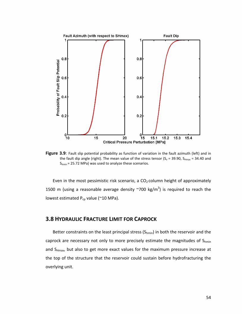
54
Figure 3.9: Fault slip potential probability as function of variation in the fault azimuth (left) and in the fault dip angle (right). The mean value of the stress tensor (Sv = 39.90, SHmax = 34.40 and Shmin = 25.72 MPa) was used to analyze these scenarios.
Even in the most pessimistic risk scenario, a CO2 column height of approximately
1500 m (using a reasonable average density ~700 kg/m3) is required to reach the
lowest estimated Pcp value (~10 MPa).
3.8 HYDRAULIC FRACTURE LIMIT FOR CAPROCK
Better constraints on the least principal stress (Shmin) in both the reservoir and the
caprock are necessary not only to more precisely estimate the magnitudes of Shmin
and SHmax, but also to get more exact values for the maximum pressure increase at
the top of the structure that the reservoir could sustain before hydrofracturing the
overlying unit.
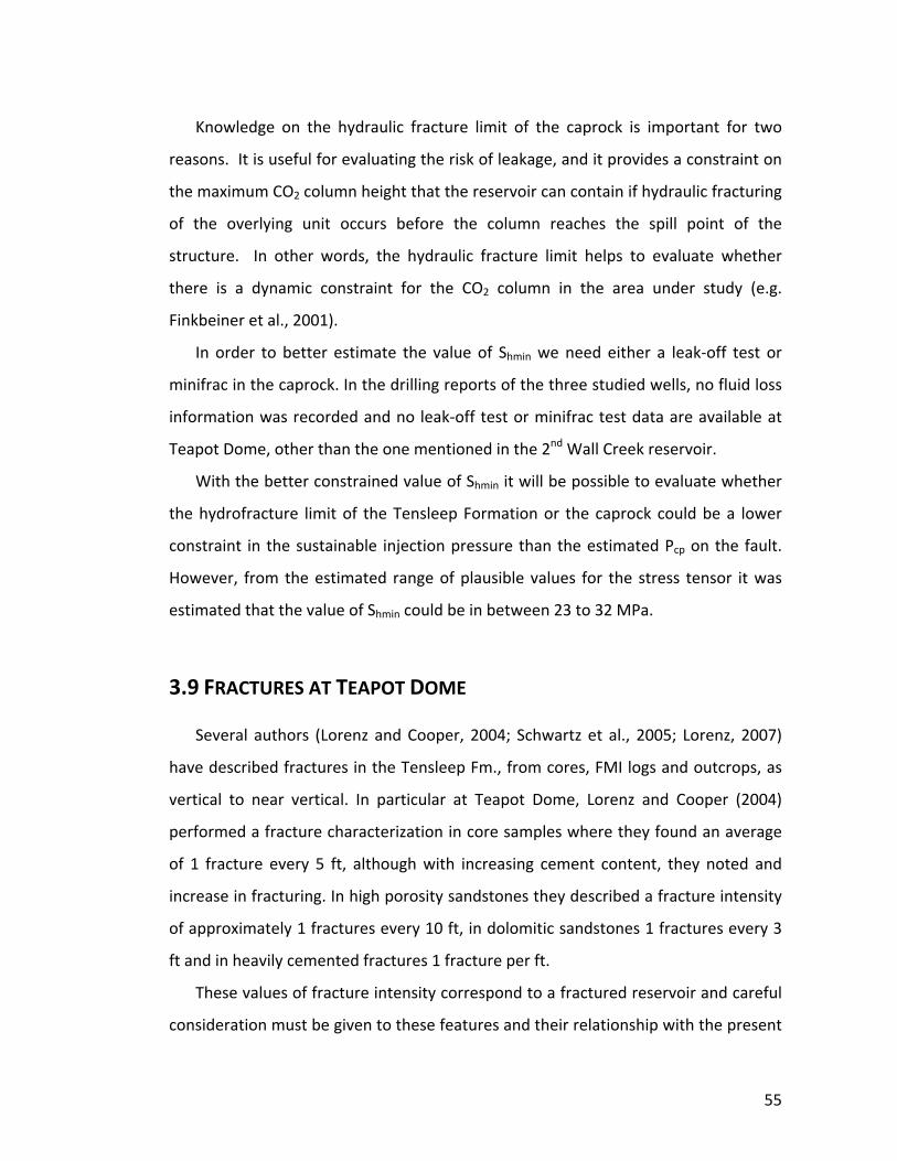
55
Knowledge on the hydraulic fracture limit of the caprock is important for two
reasons. It is useful for evaluating the risk of leakage, and it provides a constraint on
the maximum CO2 column height that the reservoir can contain if hydraulic fracturing
of the overlying unit occurs before the column reaches the spill point of the
structure. In other words, the hydraulic fracture limit helps to evaluate whether
there is a dynamic constraint for the CO2 column in the area under study (e.g.
Finkbeiner et al., 2001).
In order to better estimate the value of Shmin we need either a leak‐off test or
minifrac in the caprock. In the drilling reports of the three studied wells, no fluid loss
information was recorded and no leak‐off test or minifrac test data are available at
Teapot Dome, other than the one mentioned in the 2nd Wall Creek reservoir.
With the better constrained value of Shmin it will be possible to evaluate whether
the hydrofracture limit of the Tensleep Formation or the caprock could be a lower
constraint in the sustainable injection pressure than the estimated Pcp on the fault.
However, from the estimated range of plausible values for the stress tensor it was
estimated that the value of Shmin could be in between 23 to 32 MPa.
3.9 FRACTURES AT TEAPOT DOME
Several authors (Lorenz and Cooper, 2004; Schwartz et al., 2005; Lorenz, 2007)
have described fractures in the Tensleep Fm., from cores, FMI logs and outcrops, as
vertical to near vertical. In particular at Teapot Dome, Lorenz and Cooper (2004)
performed a fracture characterization in core samples where they found an average
of 1 fracture every 5 ft, although with increasing cement content, they noted and
increase in fracturing. In high porosity sandstones they described a fracture intensity
of approximately 1 fractures every 10 ft, in dolomitic sandstones 1 fractures every 3
ft and in heavily cemented fractures 1 fracture per ft.
These values of fracture intensity correspond to a fractured reservoir and careful
consideration must be given to these features and their relationship with the present
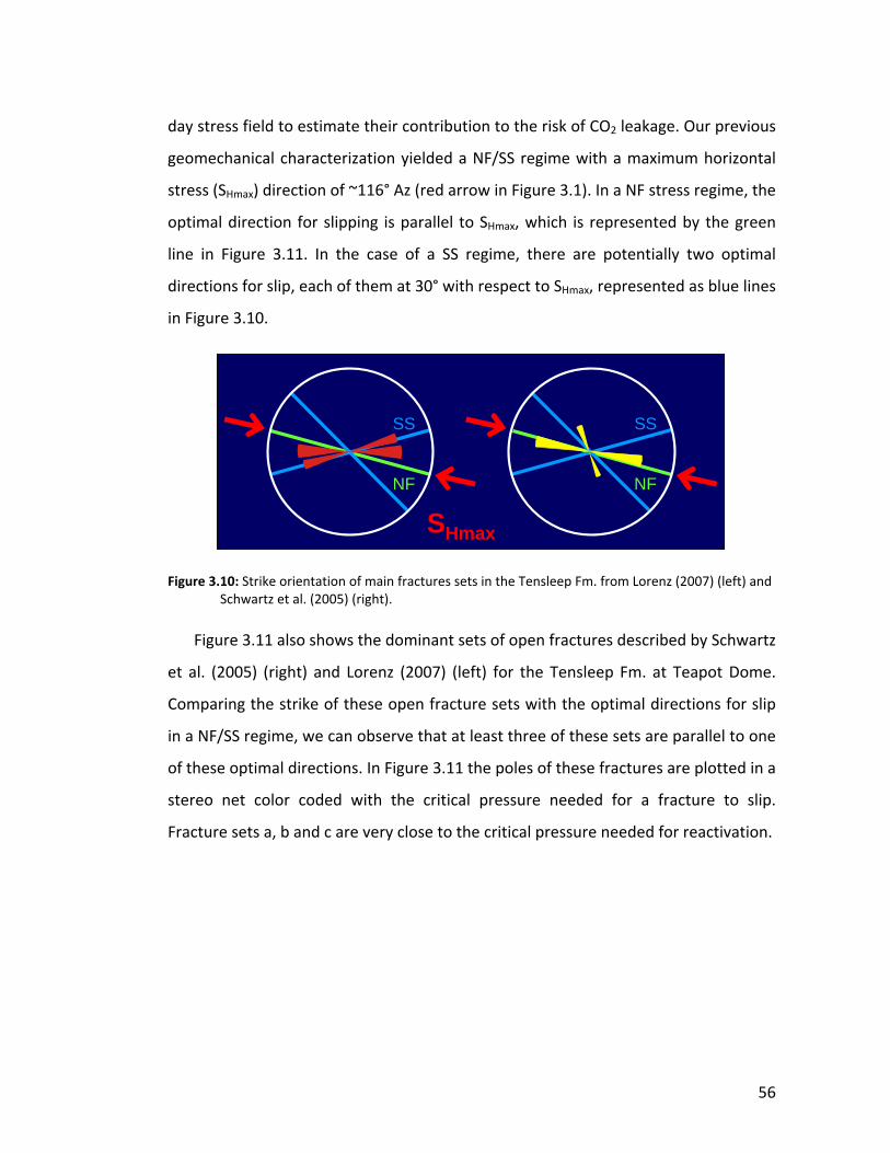
56
day stress field to estimate their contribution to the risk of CO2 leakage. Our previous
geomechanical characterization yielded a NF/SS regime with a maximum horizontal
stress (SHmax) direction of ~116° Az (red arrow in Figure 3.1). In a NF stress regime, the
optimal direction for slipping is parallel to SHmax, which is represented by the green
line in Figure 3.11. In the case of a SS regime, there are potentially two optimal
directions for slip, each of them at 30° with respect to SHmax, represented as blue lines
in Figure 3.10.
Figure 3.10: Strike orientation of main fractures sets in the Tensleep Fm. from Lorenz (2007) (left) and
Schwartz et al. (2005) (right).
Figure 3.11 also shows the dominant sets of open fractures described by Schwartz
et al. (2005) (right) and Lorenz (2007) (left) for the Tensleep Fm. at Teapot Dome.
Comparing the strike of these open fracture sets with the optimal directions for slip
in a NF/SS regime, we can observe that at least three of these sets are parallel to one
of these optimal directions. In Figure 3.11 the poles of these fractures are plotted in a
stereo net color coded with the critical pressure needed for a fracture to slip.
Fracture sets a, b and c are very close to the critical pressure needed for reactivation.
NF
SS
SHmax
NF
SS
57
Figure 3.11: Rose diagrams of the dominant fracture sets at the Tensleep Fm. (right) and the poles of
these sets color‐coded with the critical pressure needed to reactivate them (left). Note the black arrow in the bottom indicating the hydrostatic pore pressure (~16.5 MPa).
We performed a fracture characterization in the FMI logs used in the previous
sections, where we mapped several fractures sets in the reservoir as well as in the
caprock (Figure 3.12). Some of these sets coincide with previous fracture
characterizations as the ones mentioned in the previous paragraph.
d
c
b
a
MPa403020
ab
c
d
Pp MPa403020
ab
c
d
Pp
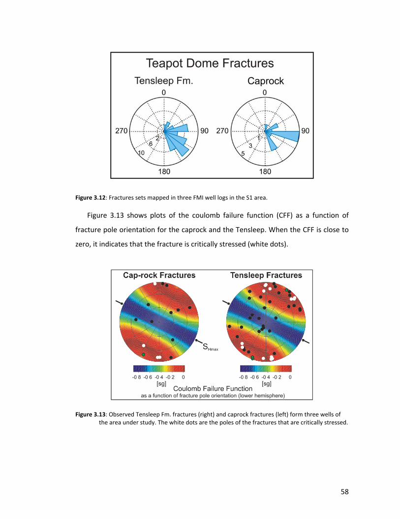
58
Figure 3.12: Fractures sets mapped in three FMI well logs in the S1 area. Figure 3.13 shows plots of the coulomb failure function (CFF) as a function of
fracture pole orientation for the caprock and the Tensleep. When the CFF is close to
zero, it indicates that the fracture is critically stressed (white dots).
Figure 3.13: Observed Tensleep Fm. fractures (right) and caprock fractures (left) form three wells of
the area under study. The white dots are the poles of the fractures that are critically stressed.

59
Several of these fractures are critically stressed, which could have a positive
impact in reservoir permeability and injectivity but constitutes a potential risk for seal
integrity, either if the caprock fractures are reactivated or if the reservoir fractures
propagate into the caprock.
If any of these two scenarios occur, the reactivation of these minor faults will
most likely result in microseismic activity. This microseismicity could be monitored to
map the vertical CO2 migration and identify potential leakages.
3.10 S2 FAULT ZONE STABILITY ANALYSIS FOR A POTENTIAL LEAKAGE
EXPERIMENT
As mentioned in the previous chapter, a second experiment has been proposed
at Teapot Dome. This second test plans to perform a controlled leakage experiment
in the S2 fault zone.
The objective is to inject small amounts of CO2 at the depth of the 2nd Wall Creek,
~930 m, in this structurally complex area, to study the potential occurrence of
leakage and methods to monitor it.
To confirm that the S2 fault area would be suitable for this experiment, we
performed a similar fault stability analysis than the one described in the previous
sections in three branches of the S2 fault. To the previous geomechanical
characterization, we incorporated drilling induced tensile fracture orientations from
wells 71‐1‐X‐4 and 48‐X‐28 (Figure 3.14) that yielded very similar stress orientations
than previously determined. Also, there is a leak‐off test in well 71‐1‐X‐4 at the depth
of the 2nd Wall Creek that confirms the NF‐SS present day stress tensor.
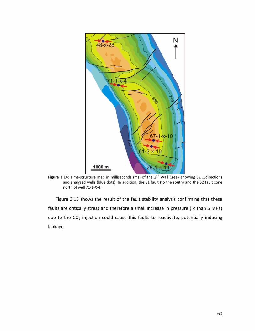
60
Figure 3.14: Time‐structure map in milliseconds (ms) of the 2nd Wall Creek showing SHmax directions and analyzed wells (blue dots). In addition, the S1 fault (to the south) and the S2 fault zone north of well 71‐1‐X‐4.
Figure 3.15 shows the result of the fault stability analysis confirming that these
faults are critically stress and therefore a small increase in pressure ( < than 5 MPa)
due to the CO2 injection could cause this faults to reactivate, potentially inducing
leakage.
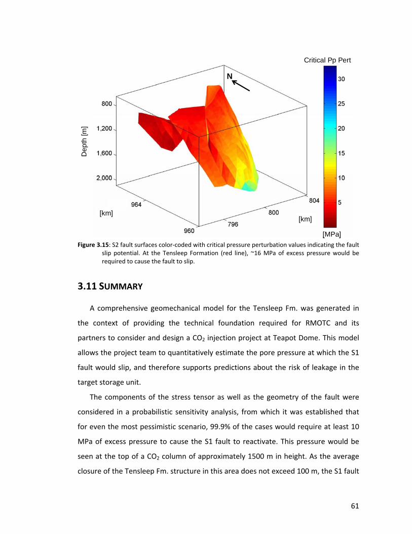
61
Figure 3.15: S2 fault surfaces color‐coded with critical pressure perturbation values indicating the fault slip potential. At the Tensleep Formation (red line), ~16 MPa of excess pressure would be required to cause the fault to slip.
3.11 SUMMARY
A comprehensive geomechanical model for the Tensleep Fm. was generated in
the context of providing the technical foundation required for RMOTC and its
partners to consider and design a CO2 injection project at Teapot Dome. This model
allows the project team to quantitatively estimate the pore pressure at which the S1
fault would slip, and therefore supports predictions about the risk of leakage in the
target storage unit.
The components of the stress tensor as well as the geometry of the fault were
considered in a probabilistic sensitivity analysis, from which it was established that
for even the most pessimistic scenario, 99.9% of the cases would require at least 10
MPa of excess pressure to cause the S1 fault to reactivate. This pressure would be
seen at the top of a CO2 column of approximately 1500 m in height. As the average
closure of the Tensleep Fm. structure in this area does not exceed 100 m, the S1 fault
[km]
[MPa]
Critical Pp Pert
ND
epth
[m]
[km][km]
[MPa]
Critical Pp Pert
ND
epth
[m]
[km]
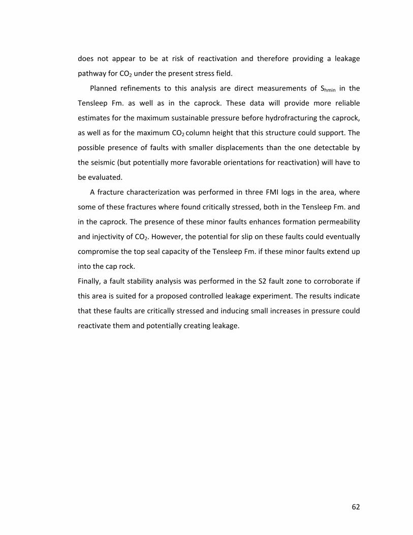
62
does not appear to be at risk of reactivation and therefore providing a leakage
pathway for CO2 under the present stress field.
Planned refinements to this analysis are direct measurements of Shmin in the
Tensleep Fm. as well as in the caprock. These data will provide more reliable
estimates for the maximum sustainable pressure before hydrofracturing the caprock,
as well as for the maximum CO2 column height that this structure could support. The
possible presence of faults with smaller displacements than the one detectable by
the seismic (but potentially more favorable orientations for reactivation) will have to
be evaluated.
A fracture characterization was performed in three FMI logs in the area, where
some of these fractures where found critically stressed, both in the Tensleep Fm. and
in the caprock. The presence of these minor faults enhances formation permeability
and injectivity of CO2. However, the potential for slip on these faults could eventually
compromise the top seal capacity of the Tensleep Fm. if these minor faults extend up
into the cap rock.
Finally, a fault stability analysis was performed in the S2 fault zone to corroborate if
this area is suited for a proposed controlled leakage experiment. The results indicate
that these faults are critically stressed and inducing small increases in pressure could
reactivate them and potentially creating leakage.
63
CHAPTER 4
3D STOCHASTIC RESERVOIR MODEL
AND FLUID FLOW SIMULATION OF THE
TENSLEEP FORMATION
4.1 ABSTRACT
Mature oil and gas reservoirs are attractive targets for geological sequestration of
CO2 because of their potential storage capacities and the possible cost offsets from
enhanced oil recovery (EOR).
In this work, we develop a 3D reservoir model and fluid flow simulation of the
Tensleep Formation using geomechanical constraints in advance of a proposed CO2‐
EOR and sequestration pilot at Teapot Dome Oil Field, WY. The objective of this work
is to model the migration of the injected CO2 as well as to obtain limits on the rates
and volumes of CO2 that can be injected, without compromising seal integrity.

64
In the present chapter, we combine our previous geomechanical analysis,
geostatistical reservoir modeling, and fluid flow simulations to investigate critical
questions regarding the feasibility of the CO2‐EOR and sequestration project in the
Tensleep Fm. The analysis takes in consideration the initial trapping and sealing
mechanisms of the reservoir, the consequences of past and present oil production on
the system, and the potential effect of the CO2 injection on the reservoir and the seal.
Finally, we also assess the storage capacity of the Tensleep Fm. in this particular trap.
The EOR and sequestration project will consist in the injection of 1 million cubic
feet (MMcfd) of supercritical CO2 for six weeks. The results of the simulations indicate
that the injected CO2 will rapidly rise to the top layers, above the main producing
interval, and will accumulate in the fractures (almost none will get into the matrix). A
well control strategy, consisting of shutting in and re opening wells, will be necessary
to improve oil recovery without circulating CO2. Incremental oil production is
predicted to be less than 10% and this value could go up to almost 30% if double the
amount of CO2 is injected in twice the amount of time.
The results suggest that the present trap could eventually hold 2 wells injecting 1
MMcfd each, during 15 years. This will sequester ~5x10⁵ tonnes of CO2 corresponding
to a small power plant of ~37,800 tonnes per year.
A sensitivity analysis was conducted to estimate the response of the pilot
performance to several parameters such as fracture permeability, porosity and
spacing, relative permeability curves, matrix porosity and permeability, and grid size.
However, in the present scheme of well control, when wells shut‐in at different times
in each scenario, that changes the distribution of the CO2 and the conditions of the
simulation. This also affects the resultant oil production and complicates the direct
comparison among scenarios. Therefore, a different approach to the sensitivity
analysis is also taken, where there is no limit on the amount of gas that each well can
produce. This approach allows comparing the impact on the system of each of the
analyzed parameters, but it does not allow comparing the amount of produced oil or
sequestered CO2.
65
4.2 INTRODUCTION
In previous stages of this project, the Tensleep Formation has been analytically
evaluated as the target horizon for a pilot CO2‐EOR and carbon storage experiment in
a three‐way closure trap against a bounding fault, termed the S1 fault. From the
comprehensive geomechanical analysis, we estimated the geomechanical constraints
we use in the fluid flow simulation described in this chapter.
It was found that the S1 fault does not appear to be at risk of reactivation and it
was estimated that caprock integrity is not a risk by the buoyancy pressure of the
maximum CO2 column height that the formation can hold. Besides, we established
the presence of critically stressed minor faults and fractures in the reservoir and
caprock. If these minor faults are reactivated, they could enhance the permeability of
the reservoir, creating permeability anisotropy inside it.
In this chapter, we develop a stochastic 3D reservoir model of the Tensleep
Formation, as input of a fluid flow simulation, using these geomechanical constraints.
Our objective is to model the migration of the injected CO2, as well as to obtain limits
on the rates and volumes of CO2 that can be injected, without compromising seal
integrity.
4.3 3D STOCHASTIC RESERVOIR MODEL
In the lifetime of an oil field, models play a fundamental role in understanding
and predicting the main geological, geophysical, and engineering reservoir
components. Reservoir modeling is never a goal on its own. It takes the geological
model as an input and delivers a product that will then be the input for a flow
simulation. Good model building requires focus on the end goal, whether it is the
estimation of the original oil in place (OOIP), the optimal placement of a well, the
design of secondary recovery methods, the prediction of water breakthrough, or the
optimization of a CO2‐EOR and Sequestration project, etc. (Caers, 2005).
66
The objective of 3D modeling is to provide one or several alternative numerical
models intended to represent those geological, geophysical and reservoir
engineering aspects of the subsurface that matter for the particular goal of the study.
These numerical models are used to estimate key reservoir parameters, predict
production performance, and provide uncertainty statements when needed. The
uncertainty statements of these reservoir parameters are as important as providing
estimates of the parameters themselves (Caers, 2005). A stochastic simulation will
provide different equiprobable numerical reservoir models (different realizations)
that when processed by the flow simulator will yield a distribution of reservoir
forecasts. This allows the transfer of uncertainty from the geological/petrophysical
model to the final forecast (Journel, 1994).
Gringarten (2005) summarized the main parts involved in stochastic 3D modeling,
which consist of a series of hierarchical steps starting with the visualization and
analysis of the data, followed by building the structural model, creating a velocity
model to perform the time‐depth conversion, and gridding the structural model.
Once the reservoir is gridded, geostatistics is used to populate the grid with the
petrophysical reservoir properties. A common applied technique in this step is
Sequential Gaussian Simulation (SGS), which is a simple method for simulating
continuous properties (porosity, permeability) requiring only knowledge of a
variogram and histogram (Caers, 2005). In this simulation process, numerous equally
probable realizations are created to quantify the uncertainty of the model. The final
step once the grid is populated is to upscale it to the chosen flow simulation grid. In
the present study, this process was carried out with a commercial software
application: Earth Decision Suite 2.1.6 – Gocad.
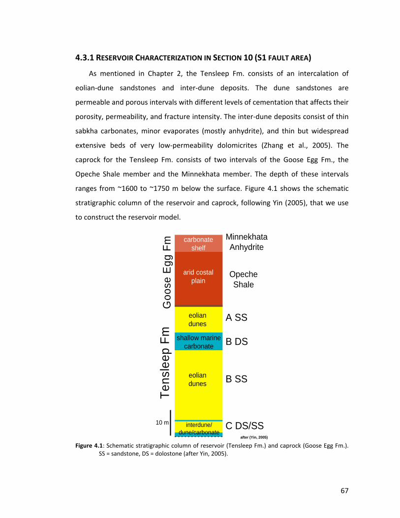
67
4.3.1 RESERVOIR CHARACTERIZATION IN SECTION 10 (S1 FAULT AREA)
As mentioned in Chapter 2, the Tensleep Fm. consists of an intercalation of
eolian‐dune sandstones and inter‐dune deposits. The dune sandstones are
permeable and porous intervals with different levels of cementation that affects their
porosity, permeability, and fracture intensity. The inter‐dune deposits consist of thin
sabkha carbonates, minor evaporates (mostly anhydrite), and thin but widespread
extensive beds of very low‐permeability dolomicrites (Zhang et al., 2005). The
caprock for the Tensleep Fm. consists of two intervals of the Goose Egg Fm., the
Opeche Shale member and the Minnekhata member. The depth of these intervals
ranges from ~1600 to ~1750 m below the surface. Figure 4.1 shows the schematic
stratigraphic column of the reservoir and caprock, following Yin (2005), that we use
to construct the reservoir model.
Figure 4.1: Schematic stratigraphic column of reservoir (Tensleep Fm.) and caprock (Goose Egg Fm.). SS = sandstone, DS = dolostone (after Yin, 2005).
Tens
leep
FmG
oose
Egg
Fm Minnekhata
Anhydrite
OpecheShale
A SS
B SS
C DS/SS
B DS
after (Yin, 2005)
carbonateshelf
arid costalplain
eoliandunes
shallow marinecarbonate
eoliandunes
interdune/dune/carbonate
10 m
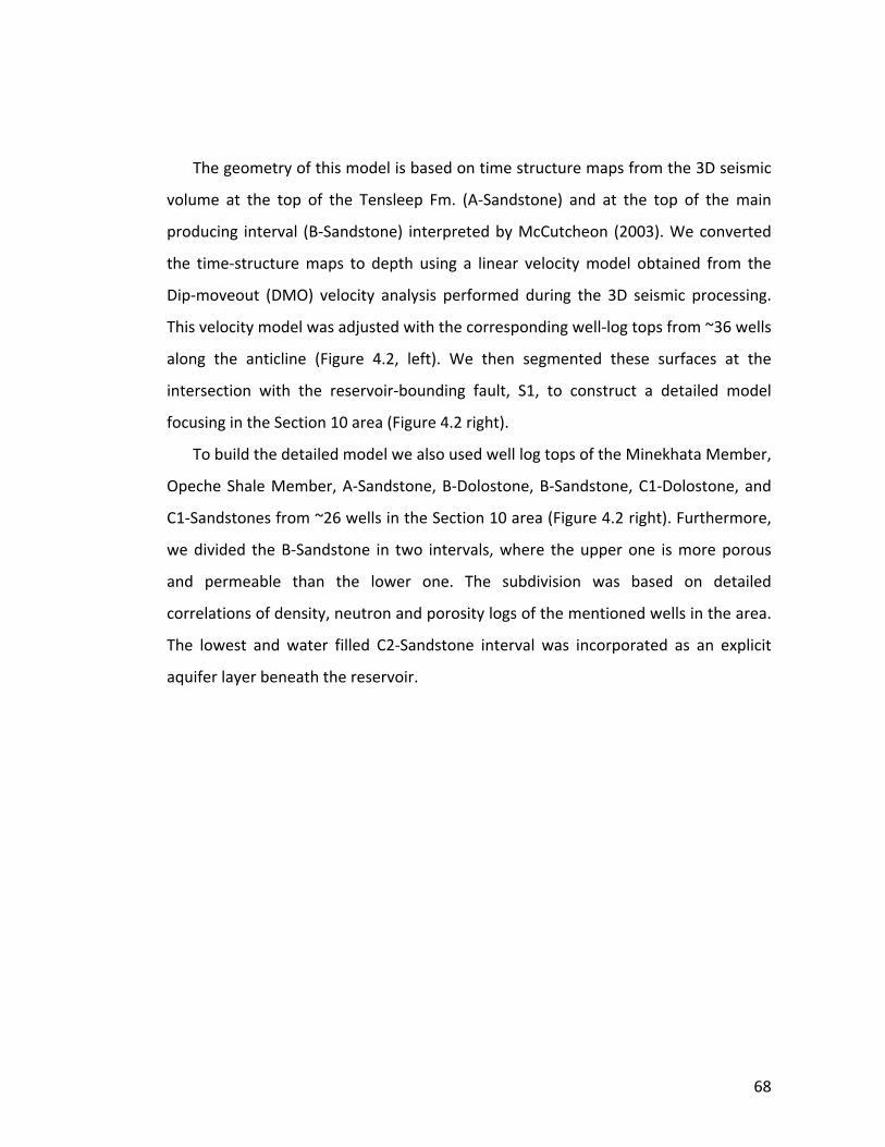
68
The geometry of this model is based on time structure maps from the 3D seismic
volume at the top of the Tensleep Fm. (A‐Sandstone) and at the top of the main
producing interval (B‐Sandstone) interpreted by McCutcheon (2003). We converted
the time‐structure maps to depth using a linear velocity model obtained from the
Dip‐moveout (DMO) velocity analysis performed during the 3D seismic processing.
This velocity model was adjusted with the corresponding well‐log tops from ~36 wells
along the anticline (Figure 4.2, left). We then segmented these surfaces at the
intersection with the reservoir‐bounding fault, S1, to construct a detailed model
focusing in the Section 10 area (Figure 4.2 right).
To build the detailed model we also used well log tops of the Minekhata Member,
Opeche Shale Member, A‐Sandstone, B‐Dolostone, B‐Sandstone, C1‐Dolostone, and
C1‐Sandstones from ~26 wells in the Section 10 area (Figure 4.2 right). Furthermore,
we divided the B‐Sandstone in two intervals, where the upper one is more porous
and permeable than the lower one. The subdivision was based on detailed
correlations of density, neutron and porosity logs of the mentioned wells in the area.
The lowest and water filled C2‐Sandstone interval was incorporated as an explicit
aquifer layer beneath the reservoir.
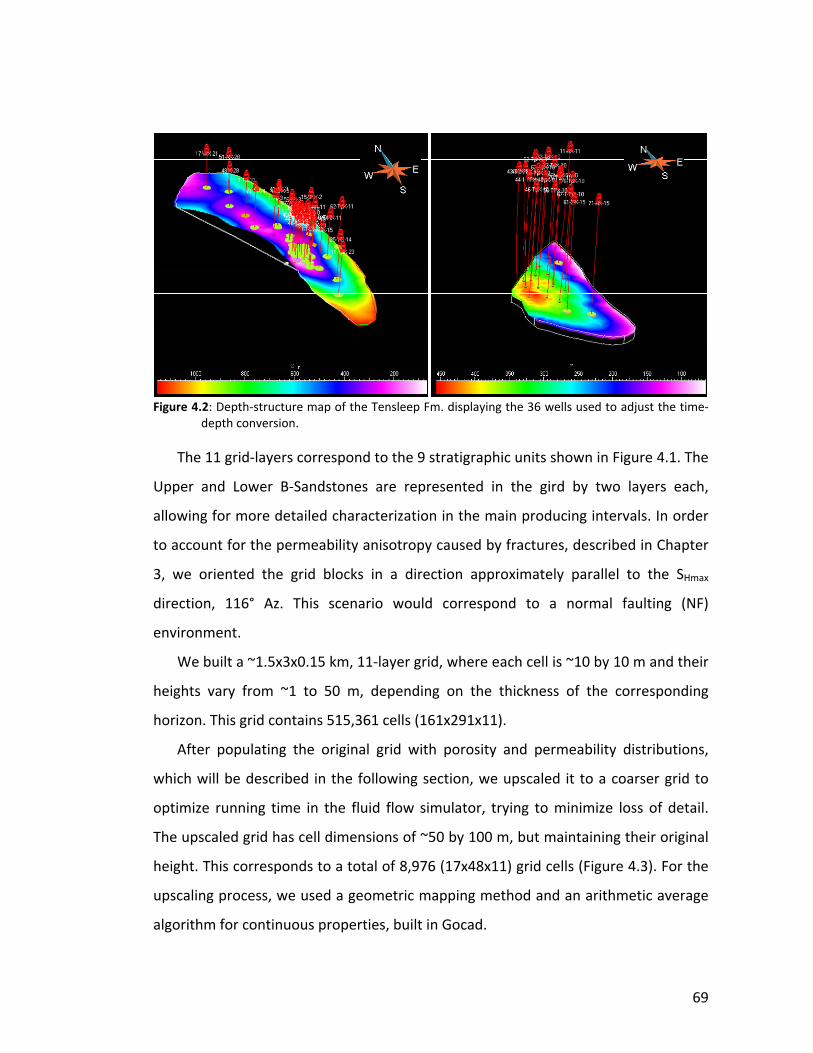
69
Figure 4.2: Depth‐structure map of the Tensleep Fm. displaying the 36 wells used to adjust the time‐depth conversion.
The 11 grid‐layers correspond to the 9 stratigraphic units shown in Figure 4.1. The
Upper and Lower B‐Sandstones are represented in the gird by two layers each,
allowing for more detailed characterization in the main producing intervals. In order
to account for the permeability anisotropy caused by fractures, described in Chapter
3, we oriented the grid blocks in a direction approximately parallel to the SHmax
direction, 116° Az. This scenario would correspond to a normal faulting (NF)
environment.
We built a ~1.5x3x0.15 km, 11‐layer grid, where each cell is ~10 by 10 m and their
heights vary from ~1 to 50 m, depending on the thickness of the corresponding
horizon. This grid contains 515,361 cells (161x291x11).
After populating the original grid with porosity and permeability distributions,
which will be described in the following section, we upscaled it to a coarser grid to
optimize running time in the fluid flow simulator, trying to minimize loss of detail.
The upscaled grid has cell dimensions of ~50 by 100 m, but maintaining their original
height. This corresponds to a total of 8,976 (17x48x11) grid cells (Figure 4.3). For the
upscaling process, we used a geometric mapping method and an arithmetic average
algorithm for continuous properties, built in Gocad.
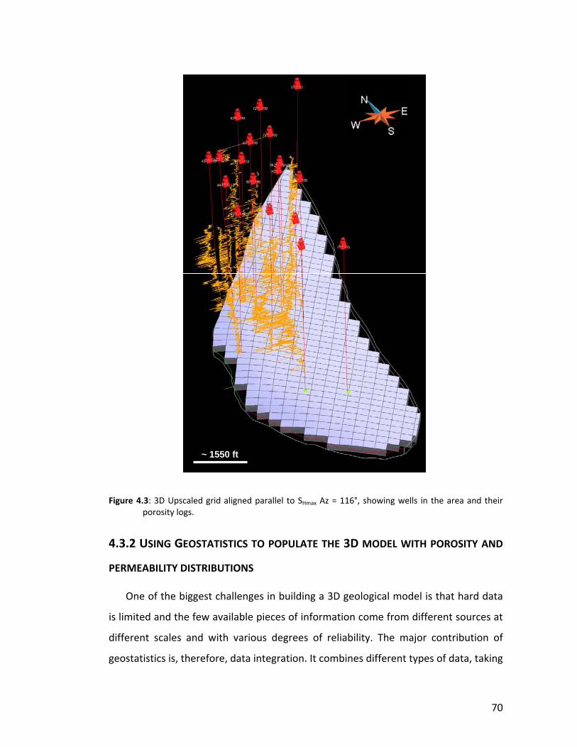
70
Figure 4.3: 3D Upscaled grid aligned parallel to SHmax Az = 116°, showing wells in the area and their porosity logs.
4.3.2 USING GEOSTATISTICS TO POPULATE THE 3D MODEL WITH POROSITY AND
PERMEABILITY DISTRIBUTIONS
One of the biggest challenges in building a 3D geological model is that hard data
is limited and the few available pieces of information come from different sources at
different scales and with various degrees of reliability. The major contribution of
geostatistics is, therefore, data integration. It combines different types of data, taking
~ 1550 ft
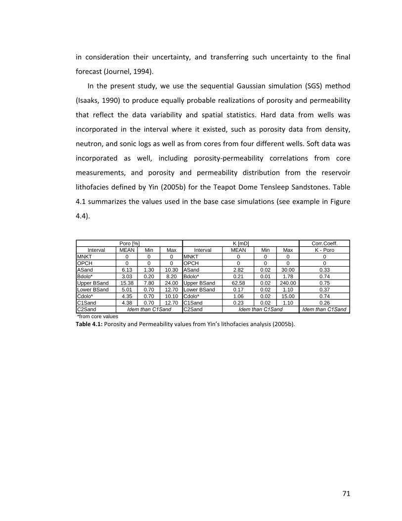
71
in consideration their uncertainty, and transferring such uncertainty to the final
forecast (Journel, 1994).
In the present study, we use the sequential Gaussian simulation (SGS) method
(Isaaks, 1990) to produce equally probable realizations of porosity and permeability
that reflect the data variability and spatial statistics. Hard data from wells was
incorporated in the interval where it existed, such as porosity data from density,
neutron, and sonic logs as well as from cores from four different wells. Soft data was
incorporated as well, including porosity‐permeability correlations from core
measurements, and porosity and permeability distribution from the reservoir
lithofacies defined by Yin (2005b) for the Teapot Dome Tensleep Sandstones. Table
4.1 summarizes the values used in the base case simulations (see example in Figure
4.4).
Table 4.1: Porosity and Permeability values from Yin’s lithofacies analysis (2005b).
Corr.Coeff.Interval MEAN Min Max Interval MEAN Min Max K - Poro
MNKT 0 0 0 MNKT 0 0 0 0OPCH 0 0 0 OPCH 0 0 0 0ASand 6.13 1.30 10.30 ASand 2.82 0.02 30.00 0.33Bdolo* 3.03 0.20 8.20 Bdolo* 0.21 0.01 1.78 0.74Upper BSand 15.38 7.80 24.00 Upper BSand 62.58 0.02 240.00 0.75Lower BSand 5.01 0.70 12.70 Lower BSand 0.17 0.02 1.10 0.37Cdolo* 4.35 0.70 10.10 Cdolo* 1.06 0.02 15.00 0.74C1Sand 4.38 0.70 12.70 C1Sand 0.23 0.02 1.10 0.26C2Sand C2Sand Idem than C1Sand*from core values
Poro [%] K [mD]
Idem than C1Sand Idem than C1Sand
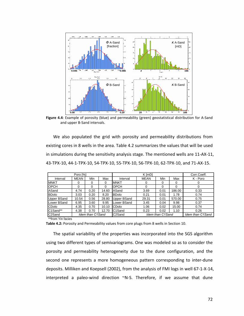
72
Figure 4.4: Example of porosity (blue) and permeability (green) geostatistical distribution for A‐Sand and upper B‐Sand intervals.
We also populated the grid with porosity and permeability distributions from
existing cores in 8 wells in the area. Table 4.2 summarizes the values that will be used
in simulations during the sensitivity analysis stage. The mentioned wells are 11‐AX‐11,
43‐TPX‐10, 44‐1‐TPX‐10, 54‐TPX‐10, 55‐TPX‐10, 56‐TPX‐10, 62‐TPX‐10, and 71‐AX‐15.
Table 4.2: Porosity and Permeability values from core plugs from 8 wells in Section 10.
The spatial variability of the properties was incorporated into the SGS algorithm
using two different types of semivariograms. One was modeled so as to consider the
porosity and permeability heterogeneity due to the dune configuration, and the
second one represents a more homogeneous pattern corresponding to inter‐dune
deposits. Milliken and Koepsell (2002), from the analysis of FMI logs in well 67‐1‐X‐14,
interpreted a paleo‐wind direction ~N‐S. Therefore, if we assume that dune
Φ A-Sand[fraction]
κ A-Sand[mD]
Φ B-Sand κ B-Sand
0.08 0.29 20 166
0.045 0.086 2 166
Corr.Coeff.Interval MEAN Min Max Interval MEAN Min Max K - Poro
MNKT 0 0 0 MNKT 0 0 0 0OPCH 0 0 0 OPCH 0 0 0 0ASand 4.74 0.20 14.60 ASand 3.69 0.01 186.00 0.33BDolo 3.03 0.20 8.20 BDolo 0.21 0.01 1.78 0.74Upper BSand 10.54 0.56 28.80 Upper BSand 29.31 0.01 570.00 0.75Lower BSand 6.95 3.60 9.95 Lower BSand 3.45 0.04 9.98 0.37CDolo 4.35 0.70 10.10 CDolo 1.06 0.02 15.00 0.74C1Sand** 4.38 0.70 12.70 C1Sand 0.23 0.02 1.10 0.26C2Sand C2Sand Idem than C1Sand**from Yin facies
Poro [%] K [mD]
Idem than C1Sand Idem than C1Sand
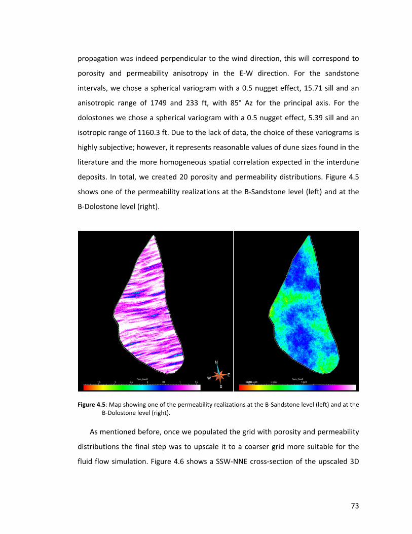
73
propagation was indeed perpendicular to the wind direction, this will correspond to
porosity and permeability anisotropy in the E‐W direction. For the sandstone
intervals, we chose a spherical variogram with a 0.5 nugget effect, 15.71 sill and an
anisotropic range of 1749 and 233 ft, with 85° Az for the principal axis. For the
dolostones we chose a spherical variogram with a 0.5 nugget effect, 5.39 sill and an
isotropic range of 1160.3 ft. Due to the lack of data, the choice of these variograms is
highly subjective; however, it represents reasonable values of dune sizes found in the
literature and the more homogeneous spatial correlation expected in the interdune
deposits. In total, we created 20 porosity and permeability distributions. Figure 4.5
shows one of the permeability realizations at the B‐Sandstone level (left) and at the
B‐Dolostone level (right).
Figure 4.5: Map showing one of the permeability realizations at the B‐Sandstone level (left) and at the
B‐Dolostone level (right). As mentioned before, once we populated the grid with porosity and permeability
distributions the final step was to upscale it to a coarser grid more suitable for the
fluid flow simulation. Figure 4.6 shows a SSW‐NNE cross‐section of the upscaled 3D
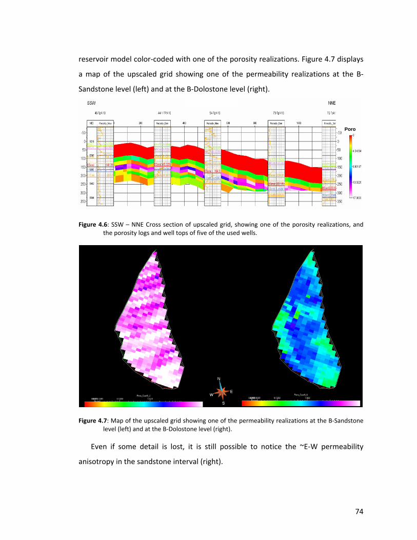
74
reservoir model color‐coded with one of the porosity realizations. Figure 4.7 displays
a map of the upscaled grid showing one of the permeability realizations at the B‐
Sandstone level (left) and at the B‐Dolostone level (right).
Figure 4.6: SSW – NNE Cross section of upscaled grid, showing one of the porosity realizations, and
the porosity logs and well tops of five of the used wells.
Figure 4.7: Map of the upscaled grid showing one of the permeability realizations at the B‐Sandstone
level (left) and at the B‐Dolostone level (right).
Even if some detail is lost, it is still possible to notice the ~E‐W permeability
anisotropy in the sandstone interval (right).
Poro
75
4.4 MODELING CO2‐EOR PROCESSES IN A FRACTURED RESERVOIR
CO2 injection has been used as a commercial process for enhanced oil recovery
(EOR) since the 1970s and is the second‐most applied EOR process in the world
(Jarrell et al., 2002). As a result, in the oil industry there is considerable experience
regarding the execution of this type of projects. Traditionally, the goal has been to
recover the higher amount of oil from the reservoir injecting the minimum amount of
gas, because the cost of CO2 affects the profitability of the project. However, when
the objective is to combine EOR and CO2 sequestration, different CO2 flooding
designs will have to be implemented in order to increase the amount of CO2 left
behind when production stops (Kovscek, 2005).
The behavior of the CO2 in the reservoir, although different from the oil behavior,
has enough similarities to allow us to use analogous techniques to better understand,
predict, and manage a CO2‐EOR project. The most common technique in practice in
the oil industry is the use of Fluid Flow Simulation, where the concept is to apply the
conservation of mass over each block of a gridded reservoir; flow rate is computed
for each of these blocks by a discrete form of Darcy’s Law (Aziz and Settari, 1979). It
considers a set of initial boundary conditions and solves second order non‐linear
partial differential equations using finite difference and/or matrix algebra (Melzer,
2007).
Some of the most commonly used simulators are based on a 3 phase, 3D, fully
implicit black oil models, but there is a number of other simulators available that
incorporate compositional or thermal effects. For example, in CO2‐EOR applications
the modified black‐oil simulator and the fully compositional simulator are the two
principal types used for predicting CO2 flood performance. The first one is an
approximate technique that accounts for oil displacement by CO2. The fully
compositional one uses an Equation‐of‐State (EOS) to predict the development of
miscibility between CO2 and oil. According to Jarrell et al. (2002), this approach is
more rigorous, but it requires more computation time.
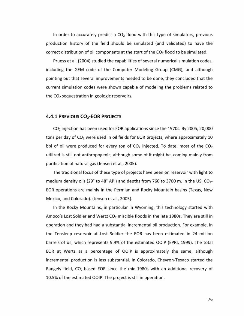
76
In order to accurately predict a CO2 flood with this type of simulators, previous
production history of the field should be simulated (and validated) to have the
correct distribution of oil components at the start of the CO2 flood to be simulated.
Pruess et al. (2004) studied the capabilities of several numerical simulation codes,
including the GEM code of the Computer Modeling Group (CMG), and although
pointing out that several improvements needed to be done, they concluded that the
current simulation codes were shown capable of modeling the problems related to
the CO2 sequestration in geologic reservoirs.
4.4.1 PREVIOUS CO2‐EOR PROJECTS
CO2 injection has been used for EOR applications since the 1970s. By 2005, 20,000
tons per day of CO2 were used in oil fields for EOR projects, where approximately 10
bbl of oil were produced for every ton of CO2 injected. To date, most of the CO2
utilized is still not anthropogenic, although some of it might be, coming mainly from
purification of natural gas (Jensen et al., 2005).
The traditional focus of these type of projects have been on reservoir with light to
medium density oils (29° to 48° API) and depths from 760 to 3700 m. In the US, CO2‐
EOR operations are mainly in the Permian and Rocky Mountain basins (Texas, New
Mexico, and Colorado). (Jensen et al., 2005).
In the Rocky Mountains, in particular in Wyoming, this technology started with
Amoco’s Lost Soldier and Wertz CO2 miscible floods in the late 1980s. They are still in
operation and they had had a substantial incremental oil production. For example, in
the Tensleep reservoir at Lost Soldier the EOR has been estimated in 24 million
barrels of oil, which represents 9.9% of the estimated OOIP (EPRI, 1999). The total
EOR at Wertz as a percentage of OOIP is approximately the same, although
incremental production is less substantial. In Colorado, Chevron‐Texaco started the
Rangely field, CO2‐based EOR since the mid‐1980s with an additional recovery of
10.5% of the estimated OOIP. The project is still in operation.
77
4.4.2 PREVIOUS FLUID FLOW SIMULATIONS AT TEAPOT DOME:
Wadleigh (2005) performed an in‐house simple reservoir simulation for RMOTC
during the first planning stages of the CO2‐EOR pilot in the Tensleep. This simulation
was done with GEM compositional simulator, which was modeled as a dual‐porosity,
dual permeability system. The equation of state (EOS) was modeled after laboratory
oil‐CO2 tests.
The grid was 14x14x5 (980 blocks) and the layers had constant porosity and
permeability values. From this model, 30 to 40% increase in oil recovery was
predicted (Friedmann and Stamp, 2006).
In the present study, we use the EOS from Wadleigh’s work.
Gaviria (2005) compared fully compositional and pseudo‐miscible black oil fluid
models to test a CO2‐EOR and sequestration project at Teapot Dome. Based on
quarter pattern simulations, he concluded that the pseudo‐miscible model could not
be used to represent the CO2 injection process in the Tensleep, and that dual porosity
models with variable fracture permeability provided a better reproduction of historic
oil and water rates; although history matching in fully‐compositional field‐scale
simulations could not be achieved.
4.4.3 CO2 PROCESS MECHANISMS
CO2 is effective for EOR operations due to its density and viscosity. At super
critical conditions, its density approaches liquid density values, but its viscosity
remains low.
CO2 and oil are multiple‐contact miscible, i.e. they require many contacts where
components of the oil and CO2 can transfer continuously. At the beginning, CO2
condenses into the oil making it lighter. Usually, methane is driven out of it. Then, the
higher components of the oil vaporize into the CO2 rich phase, making it denser and
more like the oil, therefore increasing its solubility in the oil. This process continues
until the oil‐enriched CO2 cannot be distinguished from the CO2‐enriched oil and

78
there is no interface between the CO2 and the oil (one hydrocarbon phase) (Jarrel et
al., 2002).
Miscibility is a function of temperature and pressure, but in isothermal reservoirs,
only pressure becomes important. The pressure at which miscibility occurs is called
the minimum miscibility pressure (MMP).
4.4.4 OPTIONS FOR CO2 FLOOD DESIGN
There are five basic injection processes that combine continuous, alternating, and
chase fluid injection schemes (Jarrell et al, 2002) (Figure 4.8):
- Continuous CO2 injection without any other injected fluid. This is generally
used in gravity‐drainage reservoirs (CO2 injected at top of reservoir).
- Continuous CO2 chased with water, it is similar to the continuous CO2 flood
but with chase water at the end. The immiscible water displaces the mobile
and miscible CO2‐oil mix. This design is more effective in reservoirs that are
more homogeneous.
- Conventional alternating CO2 and water, chased with water: Alternating
cycles of equal volumes of CO2 and Water (WAG) at a constant gas/water
ratio (WAG ratio). At the end, a chase of continuous water is started. This
approach is used in highly stratified heterogeneous reservoirs where the goal
is to reduce the amount of CO2 entering the high‐velocity layers.
- Tapered alternating CO2 and water (sometimes chased with water): CO2 and
water are injected in alternating unequal cycles, where the water cycles are
always increasing. The purpose of this design is to reduce the purchase cost of
CO2 but it can also reduce near‐term revenues.
- Alternating CO2 and water chased with gas: This is similar to conventional
WAG, but is then chased with a less expensive gas after the total volume of
CO2 is injected. It can also be combined with water chase in between or at the

79
end of the gas chase. This option is good to avoid the use of water on water‐
sensitive lithologies.
Figure 4.8: Illustration of typical CO2 Flood designs. Cont. CO2 = Continuous CO2 flood; Cont.
CO2/Water = Continuous CO2 flood chased with water; WAG/Water = Conventional alternating CO2 and water chased with water; TWAG/Water = Tapered alternating CO2 and water chased with water; WAG/Gas = Alternating CO2 and water chased with gas (Modified from Jarrell et al, 2002).
Since the goal of our study is to co‐optimize both oil recovery and CO2
sequestration, all the options designed to reduce the amount of CO2 to inject will not
serve the objectives of this project.
With respect to the designs that use water to displace the oil‐CO2 mix, or that use
it to control mobility of the CO2, perhaps they would have been quite useful in this
project. However, it has been shown that WAG schemes do not contribute to
maximizing CO2 storage, since some of the pore space is filled with water that
otherwise could be occupied by CO2 (Kovscek and Cakici, 2005). Similarly, the
injection of water can have a negative effect in a thick highly permeable layer, since
the injected CO2 might flow to the top of the layer, while the water could gravitate to
the bottom, seriously influencing mobility ratios. In addition, even if water has little
effect on the phase equilibrium of CO2/oil, CO2 dissolution in water may prevent
80
some of the CO2 from contacting the oil and can affect the water formation volume
factor and viscosity of water, ultimately reducing the concentration of CO2 that can
contact the oil (Jarrell et al, 2002).
Therefore, we try the well control process approach that shuts in wells with CO2
breakthroughs and re‐opens them after a certain condition is given (i.e. reservoir
pressure increases or gas saturations decreases). This has been suggested as the
most successful strategy for co‐optimization in EOR and sequestrations projects
(Kovscek and Cakici, 2005).
4.5 FLUID FLOW SIMULATION
For our fluid flow simulations we use the Generalized Equation‐of‐State Model
Compositional Reservoir Simulator (GEM, version 2007.15). We initially model the
projected CO2‐EOR and sequestration pilot in the Tensleep using a continuous CO2
flood pattern. The parameters of these simulations are described in the following
sections.
4.5.1 RESERVOIR DATA
The original oil in place of the Tensleep Fm. has been estimated as 3.8 million bbls
(0.6 million m3) of oil and 11 MMscf (0.31 million m3) of natural gas. It is a lower
gravity sulfurous oil of 32 °API, of this, more than 1.8 million bbl (0.29 million m3)
have been produced together with more than 170 million bbl (27 million m3) of water.
Reservoir pressure is 16.2 MPa (2350 psi) and reservoir temperature is 88 °C (190 °F).
CO2 swelling tests suggested that a Tensleep Sandstone CO2 flood would be miscible
or near miscible. These test showed excellent response to CO2, including oil swelling
of more than 20%, interfacial tension reduction of 90%, and five fold viscosity
reduction (Friedmann and Stamp, 2006).

81
Water production rates indicate the influence of a strong aquifer that has
maintained almost constant reservoir pressure during the history of the field.
Therefore, water drive is considered as the primary producing mechanism in the
reservoir (Gaviria, 2005, Friedmann and Stamp, 2006).
Reservoir Property Value Formation Tensleep Producing area 1.8 km2 (0.7 mi2) Average Depth 1670 m (5500 ft) Gas‐oil Contact No present Water‐oil Contact ~100 m (350 ft) ss Average Matrix Permeability of Main Producing Interval
~30 mD
Average Matrix Porosity of Main Producing Interval ~10% Oil Gravity 31 °API Reservoir Temperature 88 °C (190 °F) Primary Production Mechanism Water Drive Original Reservoir Pressure ~16 MPa (2300 psi) Bubble Point Pressure 0.3 ‐ 0.5 MPa (40 ‐ 70 psi) Average Pressure at start of CO2 injection ~16 MPa (2300 psi) Solution GOR at original pressure 4 SCF/BBL Oil Viscosity at 60 °F and 42 psi 3.5 cp Minimum Miscibility Pressure (MMP) 9 MPa (1300 psi)
Table 4.3: Basic reservoir and fluid data (modified from Gaviria, 2005).
Teapot Dome field had its first production well from First Wall Creek sandstone
interval in 1908, but the development and exploration program at Teapot Dome
started only on 1976. In 1996, a high number of wells were drilled, 27 of them
targeted the Tensleep Fm. (Gaviria, 2005). Figure 4.9 shows the historical oil and
water production from the Tensleep.
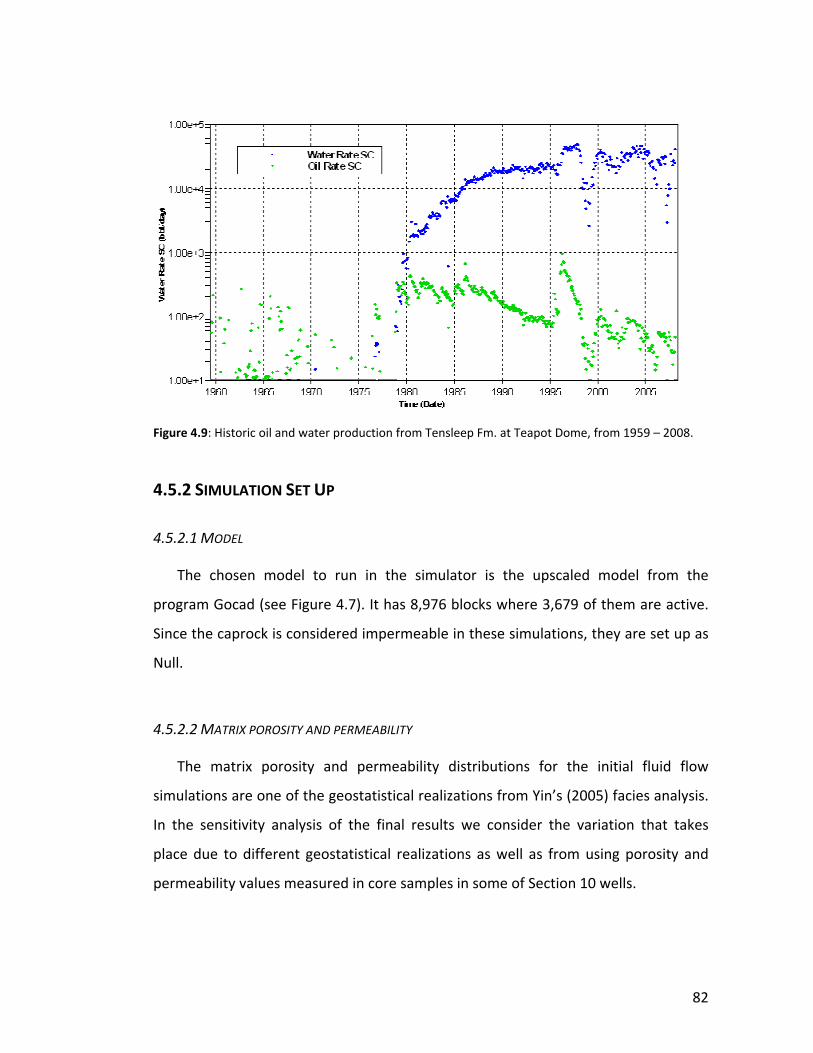
82
Figure 4.9: Historic oil and water production from Tensleep Fm. at Teapot Dome, from 1959 – 2008.
4.5.2 SIMULATION SET UP
4.5.2.1 MODEL
The chosen model to run in the simulator is the upscaled model from the
program Gocad (see Figure 4.7). It has 8,976 blocks where 3,679 of them are active.
Since the caprock is considered impermeable in these simulations, they are set up as
Null.
4.5.2.2 MATRIX POROSITY AND PERMEABILITY
The matrix porosity and permeability distributions for the initial fluid flow
simulations are one of the geostatistical realizations from Yin’s (2005) facies analysis.
In the sensitivity analysis of the final results we consider the variation that takes
place due to different geostatistical realizations as well as from using porosity and
permeability values measured in core samples in some of Section 10 wells.
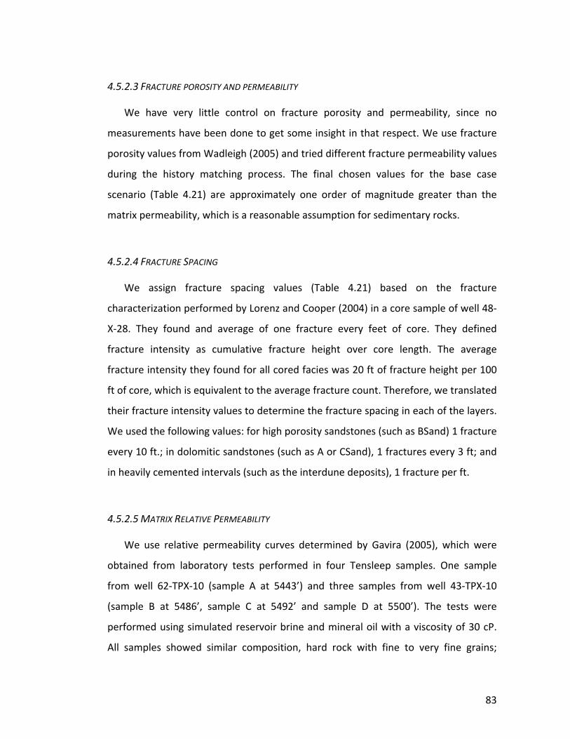
83
4.5.2.3 FRACTURE POROSITY AND PERMEABILITY
We have very little control on fracture porosity and permeability, since no
measurements have been done to get some insight in that respect. We use fracture
porosity values from Wadleigh (2005) and tried different fracture permeability values
during the history matching process. The final chosen values for the base case
scenario (Table 4.21) are approximately one order of magnitude greater than the
matrix permeability, which is a reasonable assumption for sedimentary rocks.
4.5.2.4 FRACTURE SPACING
We assign fracture spacing values (Table 4.21) based on the fracture
characterization performed by Lorenz and Cooper (2004) in a core sample of well 48‐
X‐28. They found and average of one fracture every feet of core. They defined
fracture intensity as cumulative fracture height over core length. The average
fracture intensity they found for all cored facies was 20 ft of fracture height per 100
ft of core, which is equivalent to the average fracture count. Therefore, we translated
their fracture intensity values to determine the fracture spacing in each of the layers.
We used the following values: for high porosity sandstones (such as BSand) 1 fracture
every 10 ft.; in dolomitic sandstones (such as A or CSand), 1 fractures every 3 ft; and
in heavily cemented intervals (such as the interdune deposits), 1 fracture per ft.
4.5.2.5 MATRIX RELATIVE PERMEABILITY
We use relative permeability curves determined by Gavira (2005), which were
obtained from laboratory tests performed in four Tensleep samples. One sample
from well 62‐TPX‐10 (sample A at 5443’) and three samples from well 43‐TPX‐10
(sample B at 5486’, sample C at 5492’ and sample D at 5500’). The tests were
performed using simulated reservoir brine and mineral oil with a viscosity of 30 cP.
All samples showed similar composition, hard rock with fine to very fine grains;
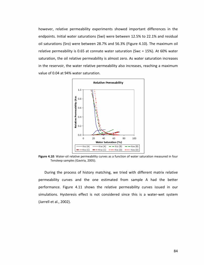
84
however, relative permeability experiments showed important differences in the
endpoints. Initial water saturations (Swi) were between 12.5% to 22.1% and residual
oil saturations (Sro) were between 28.7% and 56.3% (Figure 4.10). The maximum oil
relative permeability is 0.65 at connate water saturation (Swc = 15%). At 60% water
saturation, the oil relative permeability is almost zero. As water saturation increases
in the reservoir, the water relative permeability also increases, reaching a maximum
value of 0.04 at 94% water saturation.
Figure 4.10: Water‐oil relative permeability curves as a function of water saturation measured in four Tensleep samples (Gaviria, 2005).
During the process of history matching, we tried with different matrix relative
permeability curves and the one estimated from sample A had the better
performance. Figure 4.11 shows the relative permeability curves issued in our
simulations. Hysteresis effect is not considered since this is a water‐wet system
(Jarrell et al., 2002).
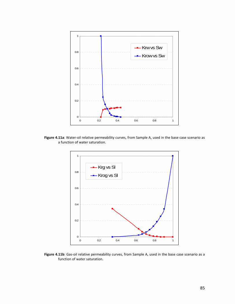
85
Figure 4.11a: Water‐oil relative permeability curves, from Sample A, used in the base case scenario as a function of water saturation.
Figure 4.11b: Gas‐oil relative permeability curves, from Sample A, used in the base case scenario as a
function of water saturation.
0
0.2
0.4
0.6
0.8
1
0 0.2 0.4 0.6 0.8 1
Krg vs Sl
Krog vs Sl
0
0.2
0.4
0.6
0.8
1
0 0.2 0.4 0.6 0.8 1
Krw vs Sw
Krow vs Sw
86
GEM allows the use of Stone's first and second models, as modified by Aziz and
Settari (1979), to obtain three phase relative permeability functions from two phase
data (GEM 2007.11, Aziz and Settari, 1979). In our simulations, we used Stone’s first
model.
4.5.2.6 FRACTURE RELATIVE PERMEABILITY
It is normally assumed that fracture relative permeability curves are straight lines;
although these might not be the best representations since fracture aperture
changes due to compaction, mineralization, and other factors that affect fluid flow.
Similarly, roughness, capillary pressure, and wettability influence fluid flow
interference. If very high fracture permeability values are considered, then straight
line relative permeability curves might be reasonable assumptions.
Since no data was available for fracture relative permeability curves, during the
history matching process we tried several arbitrary curves, close to straight lines
configuration. However, it was difficult to match the total produced water without
having to use extreme values of fracture permeabilities. Since this is an
unconstrained problem, where the only data available for history matching is historic
productions of water and oil, we decided to use the same relative permeability curve
for both matrix and fracture during the history matching stage. Later, we tested the
sensitivity on the results to different fracture permeability curves during the
prediction stage.
4.5.2.7 CO2 RELATIVE PERMEABILITY
In the case of an immiscible flood (reservoir pressure < MMP) CO2 will remain in a
gas phase which is non‐wetting compared to the oil and water. Therefore, usual
three phase relative permeability models will apply to the oil, water, and gas relative
permeabilities (Jerrell et al., 2002).

87
In the case of a miscible flood above the MMP the CO2‐rich phase is a solvent that
has similar properties to the oil and initially follows the oil relative permeability curve.
Here the solvent would be the intermediate wetting phase if the reservoir is oil‐wet,
and the solvent relative permeability will be affected by the reduction in pore space
occupied by oil and water. Or eventually, if the solvent is less wet than water, water
blocking could happen (Jerrell et al., 2002).
Since CO2 is a multiple contact solvent, when injected, it leaves behind a small
residual oil saturation that interferes with subsequent flows of solvent and causes
the solvent (CO2‐rich phase) relative permeability to be lower than the oil relative
permeability (Chopra et al., 1999, Jarrell et al, 2002). This effect was described for oil‐
wet or mixed‐wet reservoirs.
In the case of a strong water‐wet reservoir, oil is the intermediate wetting phase
and the CO2‐rich phase is the non‐wetting phase. Here the solvent relative
permeability will be reduced by residual oil.
However, measurements of steady‐state relative permeability for solvent, oil, and
water for a water‐wet dolomite showed that the solvent relative permeability was
almost the same as the oil (Dria, et al, 1993, Jerrell et al., 2002).
In a case as the present one, a water‐wet reservoir where no measurements of
solvent relative permeability are available, we assume that CO2 relative permeability
is equal to oil relative permeability, as recommended by Jerrell et al. (2002).
4.5.2.8 CAPILLARY PRESSURE
The capillary pressure (Figure 4.12) we used in our simulation is an average curve
obtained from three Tensleep samples (Gavira, 2005). Two of them were extracted
from well 56‐TPX‐10 (samples E at 5391’ and F at 5400’) and one from well 44‐1‐TPX‐
10 (sample G at 5538’). Capillary pressure curves in these three samples show low
displacement pressure (approximately 1 psi), which suggests a good reservoir with
very good sorting and big pore throats (Gaviria, 2005).
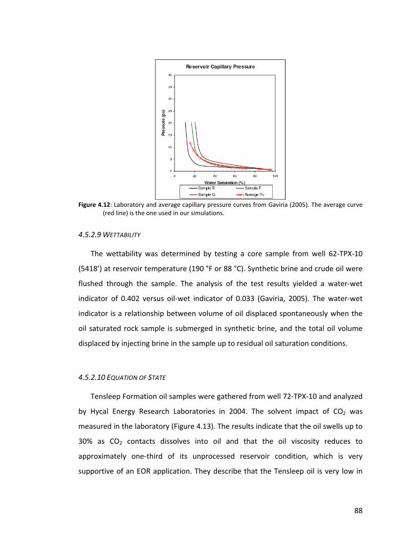
88
Figure 4.12: Laboratory and average capillary pressure curves from Gaviria (2005). The average curve (red line) is the one used in our simulations.
4.5.2.9 WETTABILITY
The wettability was determined by testing a core sample from well 62‐TPX‐10
(5418’) at reservoir temperature (190 °F or 88 °C). Synthetic brine and crude oil were
flushed through the sample. The analysis of the test results yielded a water‐wet
indicator of 0.402 versus oil‐wet indicator of 0.033 (Gaviria, 2005). The water‐wet
indicator is a relationship between volume of oil displaced spontaneously when the
oil saturated rock sample is submerged in synthetic brine, and the total oil volume
displaced by injecting brine in the sample up to residual oil saturation conditions.
4.5.2.10 EQUATION OF STATE
Tensleep Formation oil samples were gathered from well 72‐TPX‐10 and analyzed
by Hycal Energy Research Laboratories in 2004. The solvent impact of CO2 was
measured in the laboratory (Figure 4.13). The results indicate that the oil swells up to
30% as CO2 contacts dissolves into oil and that the oil viscosity reduces to
approximately one‐third of its unprocessed reservoir condition, which is very
supportive of an EOR application. They describe that the Tensleep oil is very low in
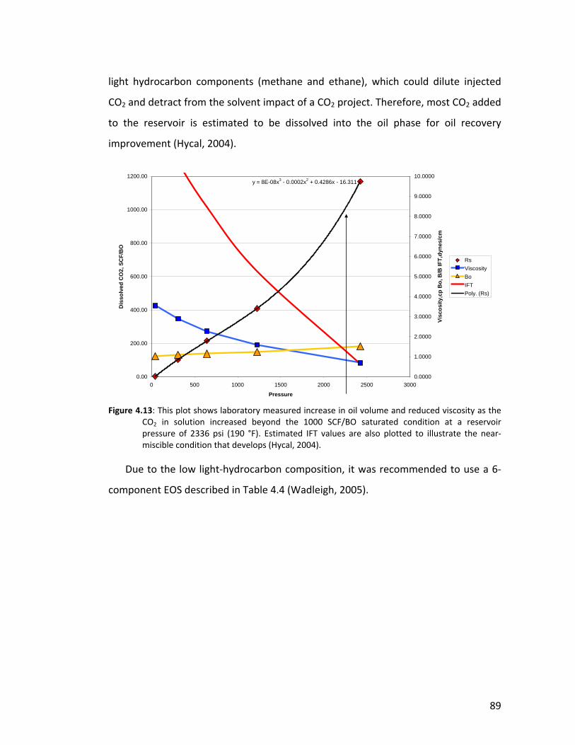
89
light hydrocarbon components (methane and ethane), which could dilute injected
CO2 and detract from the solvent impact of a CO2 project. Therefore, most CO2 added
to the reservoir is estimated to be dissolved into the oil phase for oil recovery
improvement (Hycal, 2004).
Figure 4.13: This plot shows laboratory measured increase in oil volume and reduced viscosity as the CO2 in solution increased beyond the 1000 SCF/BO saturated condition at a reservoir pressure of 2336 psi (190 °F). Estimated IFT values are also plotted to illustrate the near‐miscible condition that develops (Hycal, 2004).
Due to the low light‐hydrocarbon composition, it was recommended to use a 6‐
component EOS described in Table 4.4 (Wadleigh, 2005).
y = 8E-08x3 - 0.0002x2 + 0.4286x - 16.311
0.00
200.00
400.00
600.00
800.00
1000.00
1200.00
0 500 1000 1500 2000 2500 3000
Pressure
Dis
solv
ed C
O2,
SC
F/B
O
0.0000
1.0000
2.0000
3.0000
4.0000
5.0000
6.0000
7.0000
8.0000
9.0000
10.0000
Visc
osity
,cp
Bo,
B/B
IFT,
dyne
s/cm
RsViscosityBoIFTPoly. (Rs)
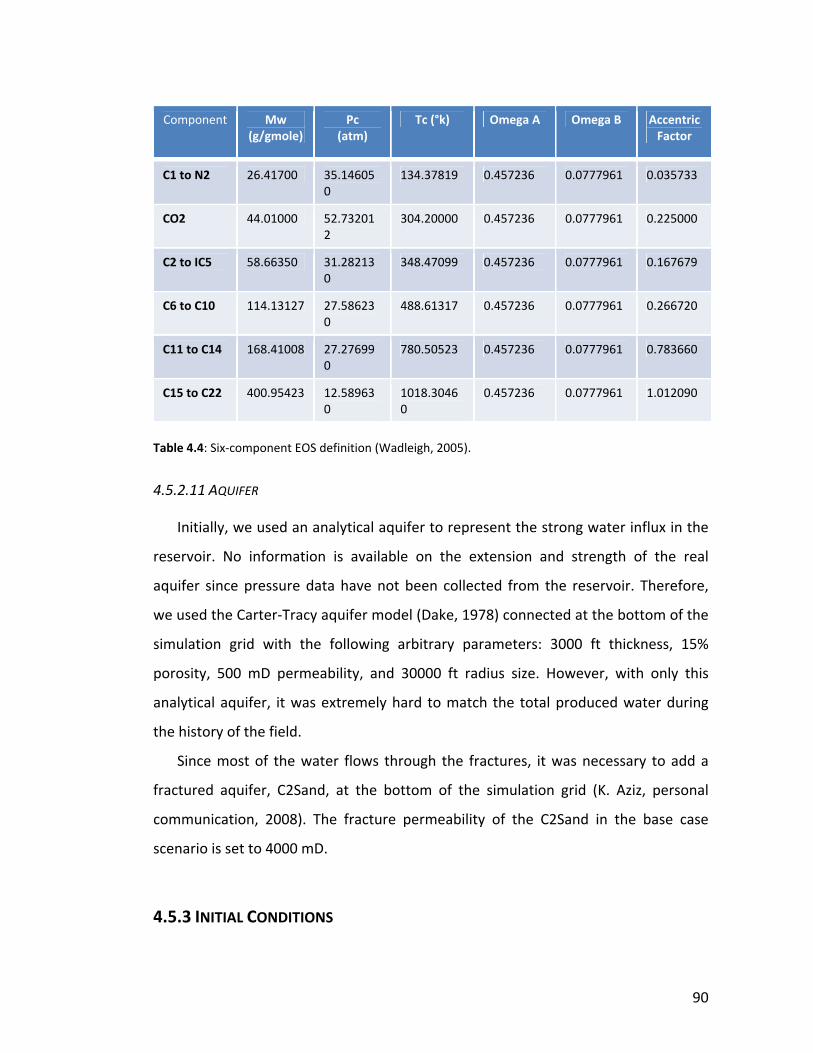
90
Component Mw (g/gmole)
Pc (atm)
Tc (°k) Omega A Omega B Accentric Factor
C1 to N2 26.41700 35.146050
134.37819 0.457236 0.0777961 0.035733
CO2 44.01000 52.732012
304.20000 0.457236 0.0777961 0.225000
C2 to IC5 58.66350 31.282130
348.47099 0.457236 0.0777961 0.167679
C6 to C10 114.13127 27.586230
488.61317 0.457236 0.0777961 0.266720
C11 to C14 168.41008 27.276990
780.50523 0.457236 0.0777961 0.783660
C15 to C22 400.95423 12.589630
1018.30460
0.457236 0.0777961 1.012090
Table 4.4: Six‐component EOS definition (Wadleigh, 2005).
4.5.2.11 AQUIFER
Initially, we used an analytical aquifer to represent the strong water influx in the
reservoir. No information is available on the extension and strength of the real
aquifer since pressure data have not been collected from the reservoir. Therefore,
we used the Carter‐Tracy aquifer model (Dake, 1978) connected at the bottom of the
simulation grid with the following arbitrary parameters: 3000 ft thickness, 15%
porosity, 500 mD permeability, and 30000 ft radius size. However, with only this
analytical aquifer, it was extremely hard to match the total produced water during
the history of the field.
Since most of the water flows through the fractures, it was necessary to add a
fractured aquifer, C2Sand, at the bottom of the simulation grid (K. Aziz, personal
communication, 2008). The fracture permeability of the C2Sand in the base case
scenario is set to 4000 mD.
4.5.3 INITIAL CONDITIONS
91
We ran the simulations in a dual porosity (dual permeability) mode.
The initial conditions were set to: reservoir pressure of 2370 psi at a reference
depth of 200 ft sub‐sea; reservoir temperature of 190 °F; oil‐water contact at 350 ft
sub‐sea. The initial water saturation from the relative permeability curve was 0.225
and the initial oil saturation within the grid blocks was 0.775.
4.5.4 HISTORY MATCHING
History matching (HM) was performed using historical oil production rates as a
constraint and comparing the simulation results to match historical water rates. The
few available pressure data in this area consists of pre‐production DST from wells 54‐
TpX‐10, 56‐TpX‐10, and 44‐1‐TpX‐10. Due to the very limited constrain in the system,
we did a HM on the production and water rates at a field scale. Therefore, sensitivity
analysis of the simulation results will be essential.
4.5.4.1 SENSITIVITY ANALYSIS TO HM PARAMETERS:
During the trial and error process of history matching we tried different
parameters such as grid size, fracture permeability (kF), fracture porosity (øF),
fracture spacing (spF), initial oil saturation (Sio), capillary pressure (Pc) and relative
permeability curves (krel). Below we present a series of sensitivity analysis that we
conducted for these parameters along the process of HM. Each parameter is
compared to one of three Scenarios, which were the best cases at the time of
performing the sensitivity analysis. All these three scenarios were run with matrix
porosity and matrix permeability from Yin’s facies analysis (see section 4.3.2); relative
permeability curves from Sample A (Figure 4.11); Sw = 0.225; oil‐water contact = 350
ft sub‐sea and the parameters shown in Table 4.5.
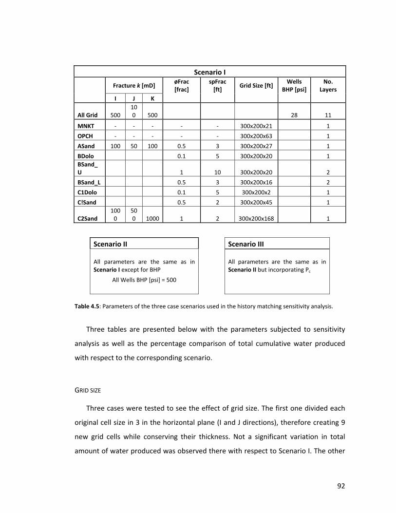
92
Scenario I
Fracture k [mD]
øFrac [frac]
spFrac [ft]
Grid Size [ft] Wells
BHP [psi] No.
Layers I J K
All Grid 500 100 500 28 11
MNKT ‐ ‐ ‐ ‐ ‐ 300x200x21 1
OPCH ‐ ‐ ‐ ‐ ‐ 300x200x63 1
ASand 100 50 100 0.5 3 300x200x27 1
BDolo 0.1 5 300x200x20 1 BSand_U 1 10 300x200x20 2
BSand_L 0.5 3 300x200x16 2
C1Dolo 0.1 5 300x200x2 1
C!Sand 0.5 2 300x200x45 1
C2Sand 1000
500 1000 1 2 300x200x168 1
Scenario II Scenario III All parameters are the same as in Scenario I except for BHP
All parameters are the same as in Scenario II but incorporating Pc
All Wells BHP [psi] = 500
Table 4.5: Parameters of the three case scenarios used in the history matching sensitivity analysis.
Three tables are presented below with the parameters subjected to sensitivity
analysis as well as the percentage comparison of total cumulative water produced
with respect to the corresponding scenario.
GRID SIZE
Three cases were tested to see the effect of grid size. The first one divided each
original cell size in 3 in the horizontal plane (I and J directions), therefore creating 9
new grid cells while conserving their thickness. Not a significant variation in total
amount of water produced was observed there with respect to Scenario I. The other
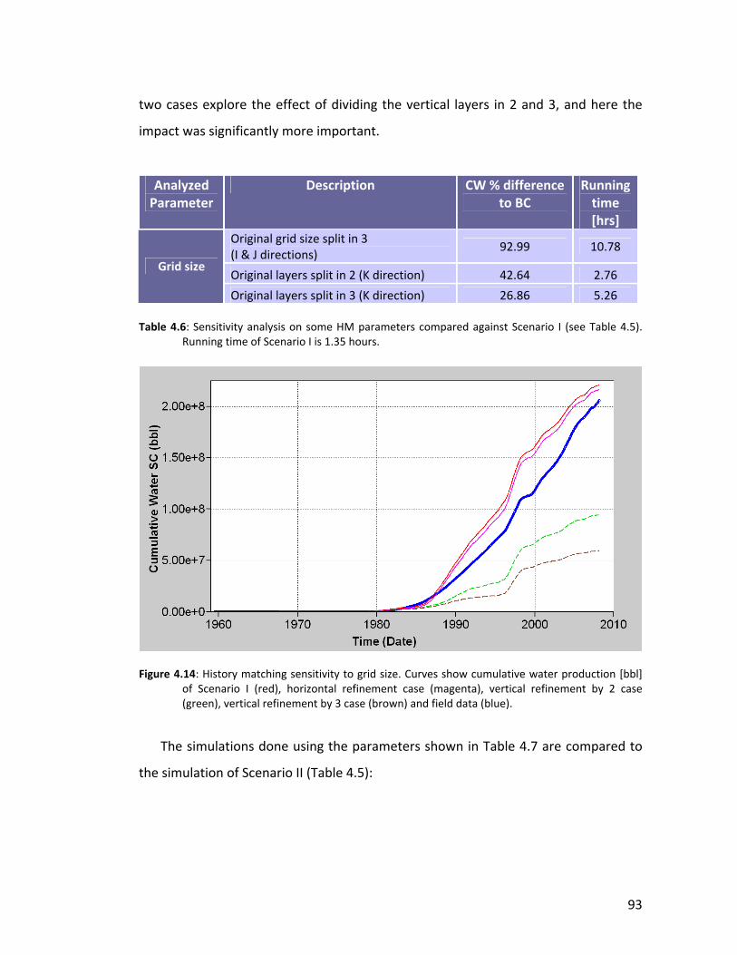
93
two cases explore the effect of dividing the vertical layers in 2 and 3, and here the
impact was significantly more important.
Analyzed Parameter
Description CW % difference to BC
Running time [hrs]
Original grid size split in 3 (I & J directions)
92.99 10.78
Original layers split in 2 (K direction) 42.64 2.76 Grid size
Original layers split in 3 (K direction) 26.86 5.26 Table 4.6: Sensitivity analysis on some HM parameters compared against Scenario I (see Table 4.5).
Running time of Scenario I is 1.35 hours.
Figure 4.14: History matching sensitivity to grid size. Curves show cumulative water production [bbl]
of Scenario I (red), horizontal refinement case (magenta), vertical refinement by 2 case (green), vertical refinement by 3 case (brown) and field data (blue).
The simulations done using the parameters shown in Table 4.7 are compared to
the simulation of Scenario II (Table 4.5):
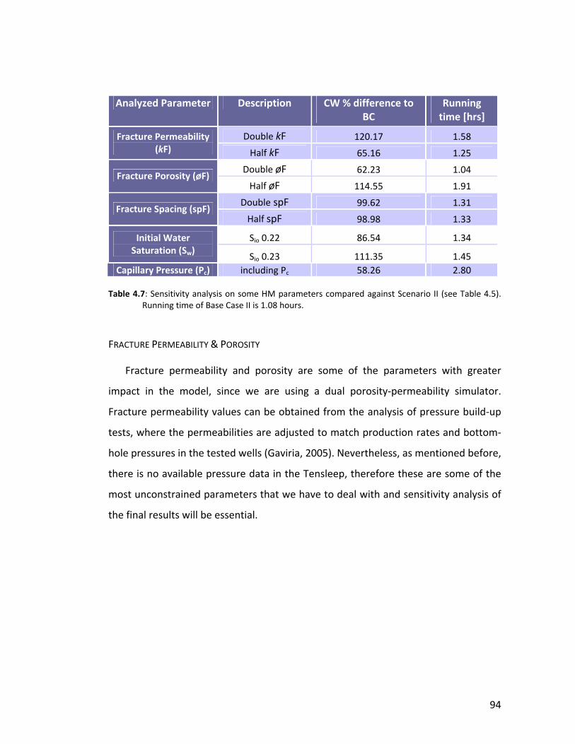
94
Analyzed Parameter Description CW % difference to BC
Running time [hrs]
Double kF 120.17 1.58 Fracture Permeability (kF) Half kF 65.16 1.25
Double øF 62.23 1.04 Fracture Porosity (øF)
Half øF 114.55 1.91
Double spF 99.62 1.31 Fracture Spacing (spF)
Half spF 98.98 1.33
Sio 0.22 86.54 1.34 Initial Water Saturation (Sw) Sio 0.23 111.35 1.45
Capillary Pressure (Pc) including Pc 58.26 2.80
Table 4.7: Sensitivity analysis on some HM parameters compared against Scenario II (see Table 4.5). Running time of Base Case II is 1.08 hours.
FRACTURE PERMEABILITY & POROSITY
Fracture permeability and porosity are some of the parameters with greater
impact in the model, since we are using a dual porosity‐permeability simulator.
Fracture permeability values can be obtained from the analysis of pressure build‐up
tests, where the permeabilities are adjusted to match production rates and bottom‐
hole pressures in the tested wells (Gaviria, 2005). Nevertheless, as mentioned before,
there is no available pressure data in the Tensleep, therefore these are some of the
most unconstrained parameters that we have to deal with and sensitivity analysis of
the final results will be essential.
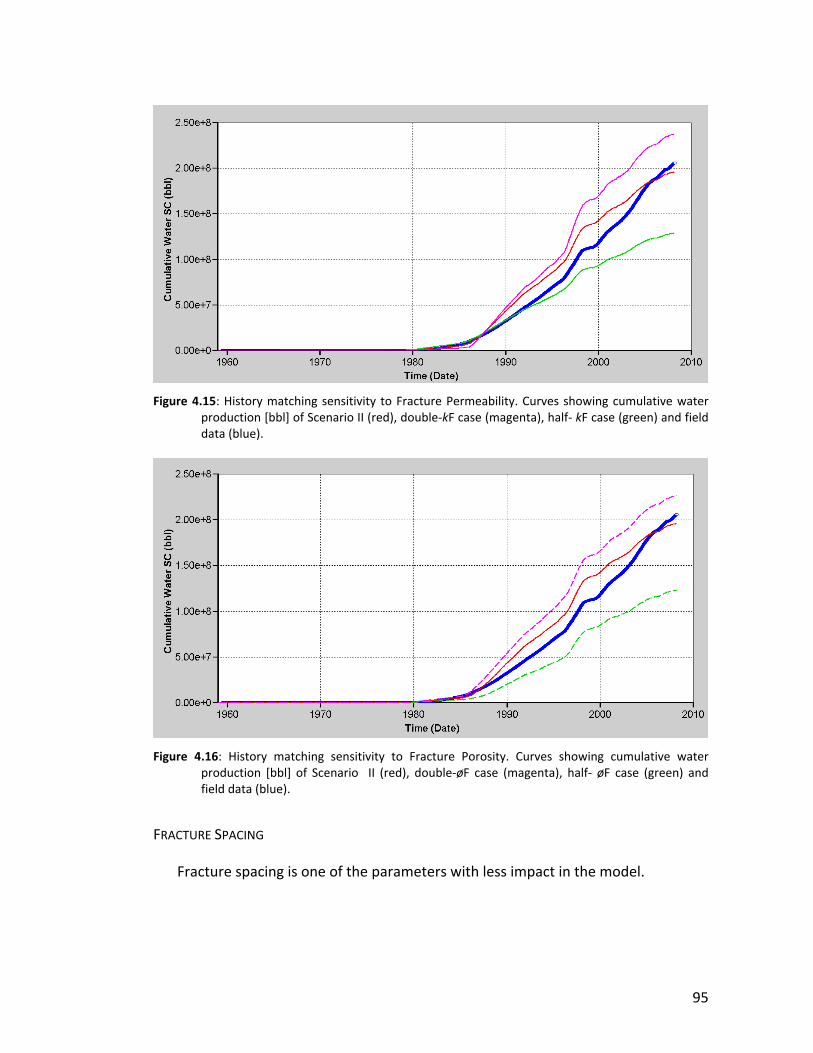
95
Figure 4.15: History matching sensitivity to Fracture Permeability. Curves showing cumulative water
production [bbl] of Scenario II (red), double‐kF case (magenta), half‐ kF case (green) and field data (blue).
Figure 4.16: History matching sensitivity to Fracture Porosity. Curves showing cumulative water
production [bbl] of Scenario II (red), double‐øF case (magenta), half‐ øF case (green) and field data (blue).
FRACTURE SPACING
Fracture spacing is one of the parameters with less impact in the model.
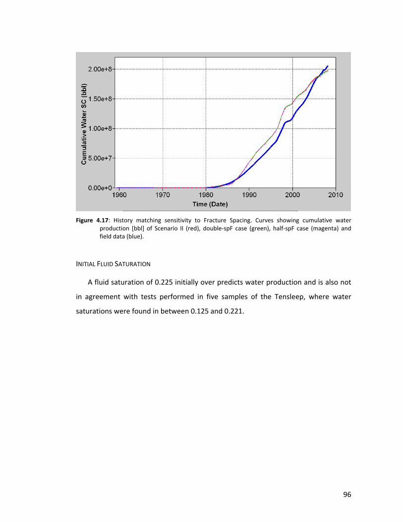
96
Figure 4.17: History matching sensitivity to Fracture Spacing. Curves showing cumulative water
production [bbl] of Scenario II (red), double‐spF case (green), half‐spF case (magenta) and field data (blue).
INITIAL FLUID SATURATION
A fluid saturation of 0.225 initially over predicts water production and is also not
in agreement with tests performed in five samples of the Tensleep, where water
saturations were found in between 0.125 and 0.221.
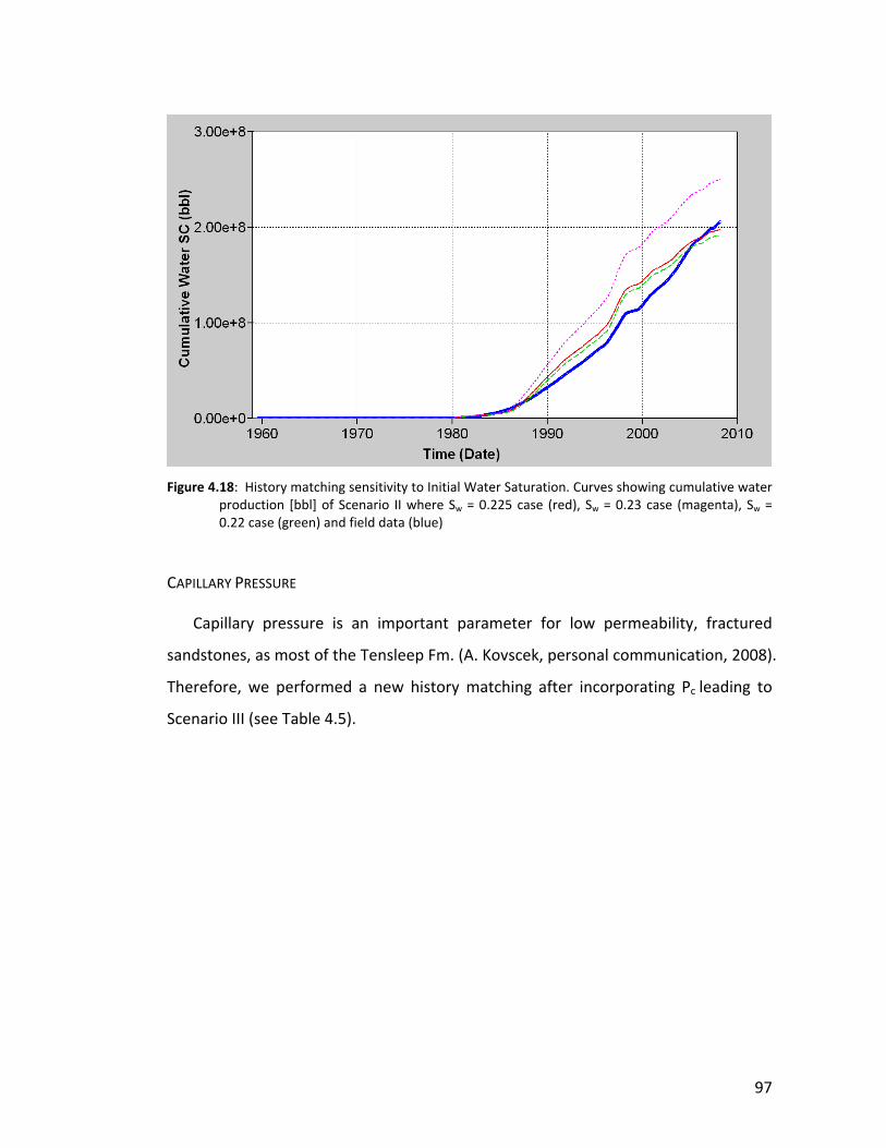
97
Figure 4.18: History matching sensitivity to Initial Water Saturation. Curves showing cumulative water
production [bbl] of Scenario II where Sw = 0.225 case (red), Sw = 0.23 case (magenta), Sw = 0.22 case (green) and field data (blue)
CAPILLARY PRESSURE
Capillary pressure is an important parameter for low permeability, fractured
sandstones, as most of the Tensleep Fm. (A. Kovscek, personal communication, 2008).
Therefore, we performed a new history matching after incorporating Pc leading to
Scenario III (see Table 4.5).
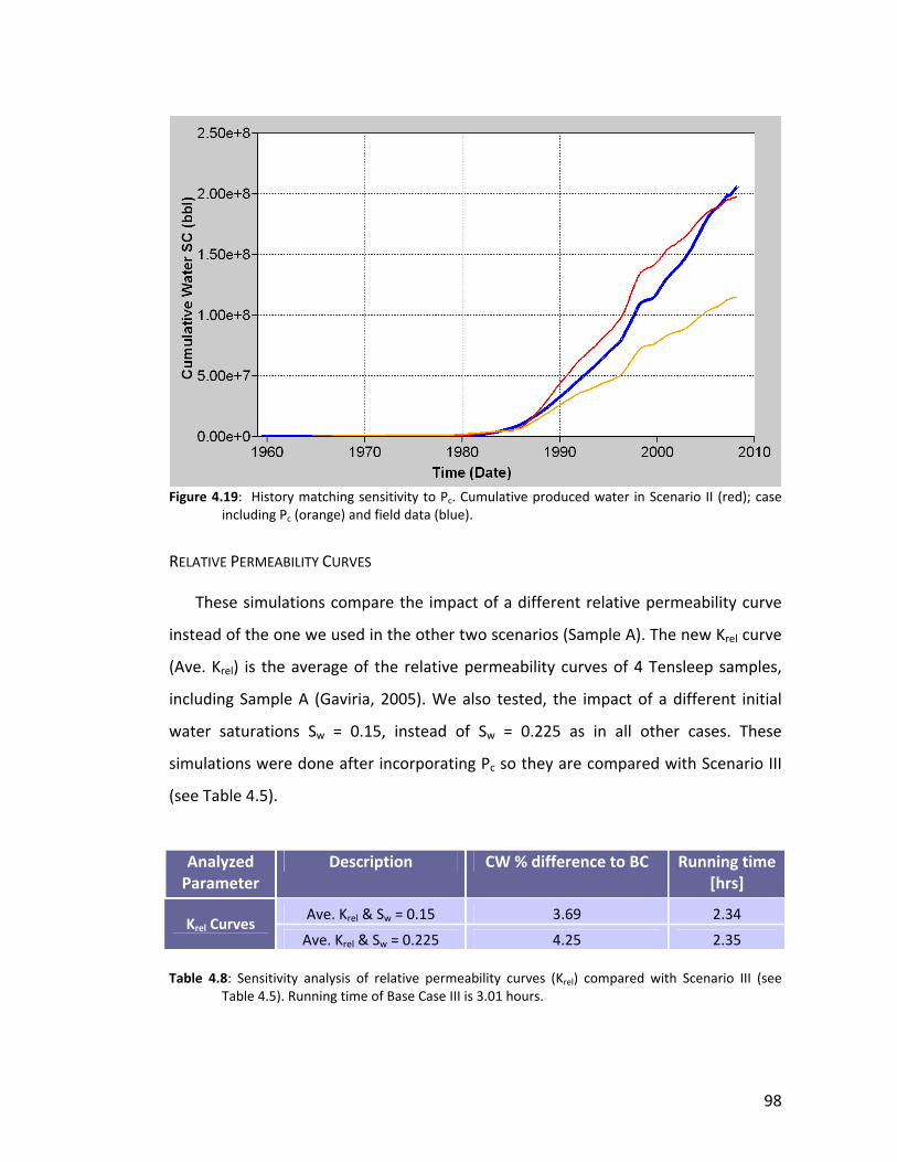
98
Figure 4.19: History matching sensitivity to Pc. Cumulative produced water in Scenario II (red); case including Pc (orange) and field data (blue).
RELATIVE PERMEABILITY CURVES
These simulations compare the impact of a different relative permeability curve
instead of the one we used in the other two scenarios (Sample A). The new Krel curve
(Ave. Krel) is the average of the relative permeability curves of 4 Tensleep samples,
including Sample A (Gaviria, 2005). We also tested, the impact of a different initial
water saturations Sw = 0.15, instead of Sw = 0.225 as in all other cases. These
simulations were done after incorporating Pc so they are compared with Scenario III
(see Table 4.5).
Analyzed Parameter
Description CW % difference to BC Running time [hrs]
Ave. Krel & Sw = 0.15 3.69 2.34 Krel Curves
Ave. Krel & Sw = 0.225 4.25 2.35 Table 4.8: Sensitivity analysis of relative permeability curves (Krel) compared with Scenario III (see
Table 4.5). Running time of Base Case III is 3.01 hours.
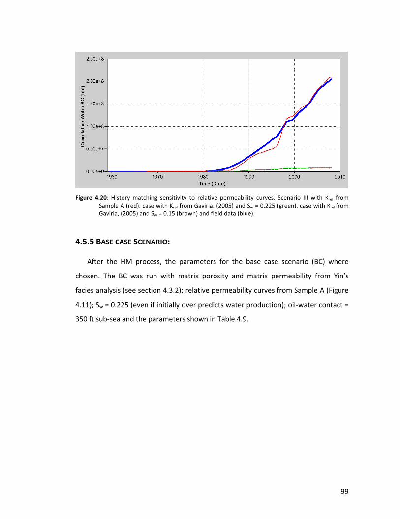
99
Figure 4.20: History matching sensitivity to relative permeability curves. Scenario III with Krel from
Sample A (red), case with Krel from Gaviria, (2005) and Sw = 0.225 (green), case with Krel from Gaviria, (2005) and Sw = 0.15 (brown) and field data (blue).
4.5.5 BASE CASE SCENARIO:
After the HM process, the parameters for the base case scenario (BC) where
chosen. The BC was run with matrix porosity and matrix permeability from Yin’s
facies analysis (see section 4.3.2); relative permeability curves from Sample A (Figure
4.11); Sw = 0.225 (even if initially over predicts water production); oil‐water contact =
350 ft sub‐sea and the parameters shown in Table 4.9.
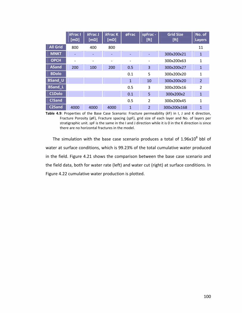
100
kFrac I [mD]
kFrac J [mD]
kFrac K [mD]
øFrac spFrac ‐ [ft]
Grid Size [ft]
No. of Layers
All Grid 800 400 800 11 MNKT ‐ ‐ ‐ ‐ ‐ 300x200x21 1 OPCH ‐ ‐ ‐ ‐ ‐ 300x200x63 1 ASand 200 100 200 0.5 3 300x200x27 1 BDolo 0.1 5 300x200x20 1
BSand_U 1 10 300x200x20 2 BSand_L 0.5 3 300x200x16 2 C1Dolo 0.1 5 300x200x2 1 C!Sand 0.5 2 300x200x45 1 C2Sand 4000 4000 4000 1 2 300x200x168 1
Table 4.9: Properties of the Base Case Scenario: Fracture permeability (kF) in I, J and K direction, Fracture Porosity (øF), Fracture spacing (spF), grid size of each layer and No. of layers per stratigraphic unit. spF is the same in the I and J direction while it is 0 in the K direction is since there are no horizontal fractures in the model.
The simulation with the base case scenario produces a total of 1.96x10⁸ bbl of
water at surface conditions, which is 99.23% of the total cumulative water produced
in the field. Figure 4.21 shows the comparison between the base case scenario and
the field data, both for water rate (left) and water cut (right) at surface conditions. In
Figure 4.22 cumulative water production is plotted.
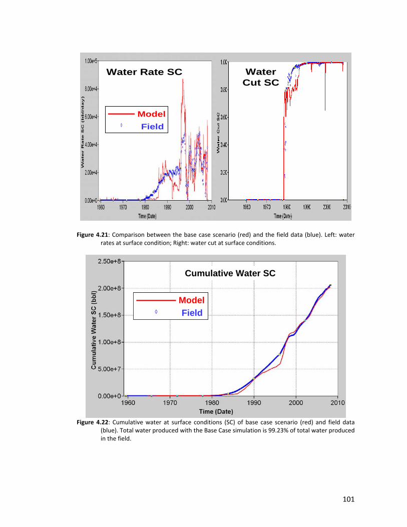
101
Figure 4.21: Comparison between the base case scenario (red) and the field data (blue). Left: water
rates at surface condition; Right: water cut at surface conditions.
Figure 4.22: Cumulative water at surface conditions (SC) of base case scenario (red) and field data (blue). Total water produced with the Base Case simulation is 99.23% of total water produced in the field.
ModelField
ModelField
Cumulative Water SC
ModelField
ModelField
Water Rate SC WaterCut SC
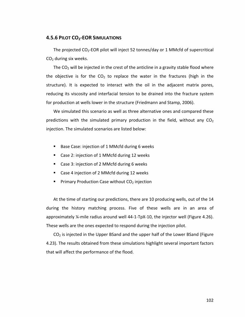
102
4.5.6 PILOT CO2‐EOR SIMULATIONS
The projected CO2‐EOR pilot will inject 52 tonnes/day or 1 MMcfd of supercritical
CO2 during six weeks.
The CO2 will be injected in the crest of the anticline in a gravity stable flood where
the objective is for the CO2 to replace the water in the fractures (high in the
structure). It is expected to interact with the oil in the adjacent matrix pores,
reducing its viscosity and interfacial tension to be drained into the fracture system
for production at wells lower in the structure (Friedmann and Stamp, 2006).
We simulated this scenario as well as three alternative ones and compared these
predictions with the simulated primary production in the field, without any CO2
injection. The simulated scenarios are listed below:
Base Case: injection of 1 MMcfd during 6 weeks
Case 2: injection of 1 MMcfd during 12 weeks
Case 3: injection of 2 MMcfd during 6 weeks
Case 4 injection of 2 MMcfd during 12 weeks
Primary Production Case without CO2 injection
At the time of starting our predictions, there are 10 producing wells, out of the 14
during the history matching process. Five of these wells are in an area of
approximately ¼‐mile radius around well 44‐1‐TpX‐10, the injector well (Figure 4.26).
These wells are the ones expected to respond during the injection pilot.
CO2 is injected in the Upper BSand and the upper half of the Lower BSand (Figure
4.23). The results obtained from these simulations highlight several important factors
that will affect the performance of the flood.
103
Figure 4.23: Injector set up. Perforations open in Upper BSand and upper layer of Lower BSand.
First, that CO2 rapidly rises (2 ‐3 days) through the highly permeable fracture
network (Figure 4.24, see crossection location on Figure 4.26) due to buoyancy forces.
It accumulates in the fractures at the top layers (ASand and BDolo) almost without
penetrating in the matrix pores. Contrary to the expected positive effect of a high
permeable fracture network, this rapid buoyancy presents a problem, since the CO2
migrates away of the main producing interval (BSand) where is being injected, and
where it was expected to remain to allow enough time to be dissolved into the oil.
44-1-X-10 (Injector)
100 ft15 ft
Pressure [MPa]
ASand
BDoloUpBSand
LowBSand
C1Sand
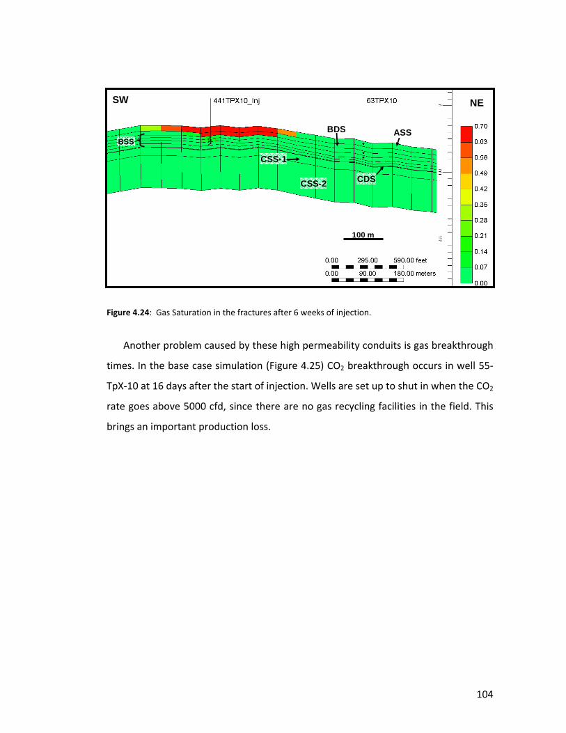
104
Figure 4.24: Gas Saturation in the fractures after 6 weeks of injection.
Another problem caused by these high permeability conduits is gas breakthrough
times. In the base case simulation (Figure 4.25) CO2 breakthrough occurs in well 55‐
TpX‐10 at 16 days after the start of injection. Wells are set up to shut in when the CO2
rate goes above 5000 cfd, since there are no gas recycling facilities in the field. This
brings an important production loss.
ASSBDSBSS
CDSCSS-2
CSS-1
100 m
SW NE
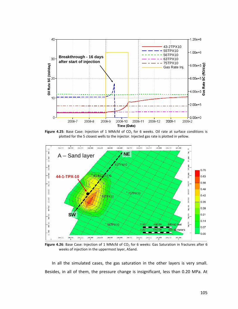
105
Figure 4.25: Base Case: Injection of 1 MMcfd of CO2 for 6 weeks. Oil rate at surface conditions is plotted for the 5 closest wells to the injector. Injected gas rate is plotted in yellow.
Figure 4.26: Base Case: Injection of 1 MMcfd of CO2 for 6 weeks: Gas Saturation in fractures after 6 weeks of injection in the uppermost layer, ASand.
In all the simulated cases, the gas saturation in the other layers is very small.
Besides, in all of them, the pressure change is insignificant, less than 0.20 MPa. At
Breakthrough - 16 days after start of injection
43-2TPX1055TPX1056TPX1063TPX1075TPX10Gas Rate Inj.
43-2TPX1055TPX1056TPX1063TPX1075TPX10Gas Rate Inj.
44-1-TPX-10
A – Sand layer
SW
NE
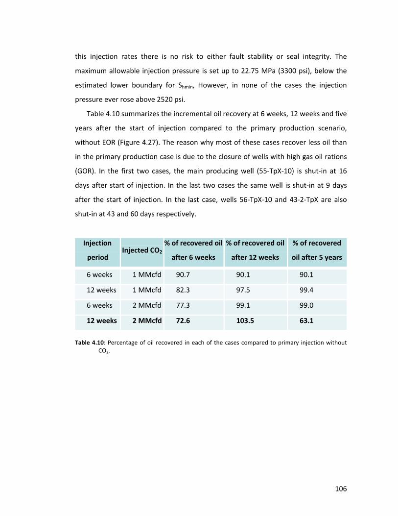
106
this injection rates there is no risk to either fault stability or seal integrity. The
maximum allowable injection pressure is set up to 22.75 MPa (3300 psi), below the
estimated lower boundary for Shmin, However, in none of the cases the injection
pressure ever rose above 2520 psi.
Table 4.10 summarizes the incremental oil recovery at 6 weeks, 12 weeks and five
years after the start of injection compared to the primary production scenario,
without EOR (Figure 4.27). The reason why most of these cases recover less oil than
in the primary production case is due to the closure of wells with high gas oil rations
(GOR). In the first two cases, the main producing well (55‐TpX‐10) is shut‐in at 16
days after start of injection. In the last two cases the same well is shut‐in at 9 days
after the start of injection. In the last case, wells 56‐TpX‐10 and 43‐2‐TpX are also
shut‐in at 43 and 60 days respectively.
Injection
period Injected CO2
% of recovered oil
after 6 weeks
% of recovered oil
after 12 weeks
% of recovered
oil after 5 years
6 weeks 1 MMcfd 90.7 90.1 90.1
12 weeks 1 MMcfd 82.3 97.5 99.4
6 weeks 2 MMcfd 77.3 99.1 99.0
12 weeks 2 MMcfd 72.6 103.5 63.1
Table 4.10: Percentage of oil recovered in each of the cases compared to primary injection without
CO2.
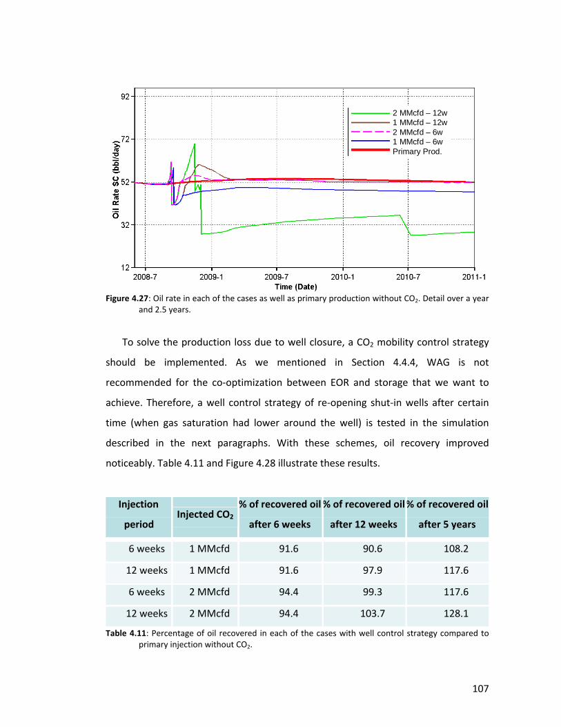
107
Figure 4.27: Oil rate in each of the cases as well as primary production without CO2. Detail over a year and 2.5 years.
To solve the production loss due to well closure, a CO2 mobility control strategy
should be implemented. As we mentioned in Section 4.4.4, WAG is not
recommended for the co‐optimization between EOR and storage that we want to
achieve. Therefore, a well control strategy of re‐opening shut‐in wells after certain
time (when gas saturation had lower around the well) is tested in the simulation
described in the next paragraphs. With these schemes, oil recovery improved
noticeably. Table 4.11 and Figure 4.28 illustrate these results.
Injection
period Injected CO2
% of recovered oil
after 6 weeks
% of recovered oil
after 12 weeks
% of recovered oil
after 5 years
6 weeks 1 MMcfd 91.6 90.6 108.2
12 weeks 1 MMcfd 91.6 97.9 117.6
6 weeks 2 MMcfd 94.4 99.3 117.6
12 weeks 2 MMcfd 94.4 103.7 128.1
Table 4.11: Percentage of oil recovered in each of the cases with well control strategy compared to primary injection without CO2.
2 MMcfd – 12w1 MMcfd – 12w2 MMcfd – 6w1 MMcfd – 6wPrimary Prod.
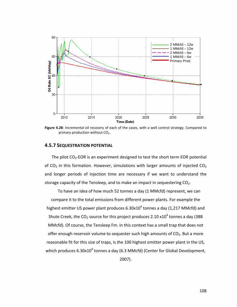
108
Figure 4.28: Incremental oil recovery of each of the cases, with a well control strategy. Compared to primary production without CO2.
4.5.7 SEQUESTRATION POTENTIAL
The pilot CO2‐EOR is an experiment designed to test the short term EOR potential
of CO2 in this formation. However, simulations with larger amounts of injected CO2
and longer periods of injection time are necessary if we want to understand the
storage capacity of the Tensleep, and to make an impact in sequestering CO2.
To have an idea of how much 52 tonnes a day (1 MMcfd) represent, we can
compare it to the total emissions from different power plants. For example the
highest emitter US power plant produces 6.30x10⁴ tonnes a day (1,217 MMcfd) and
Shute Creek, the CO2 source for this project produces 2.10 x10⁴ tonnes a day (388
MMcfd). Of course, the Tensleep Fm. in this context has a small trap that does not
offer enough reservoir volume to sequester such high amounts of CO2. But a more
reasonable fit for this size of traps, is the 100 highest emitter power plant in the US,
which produces 6.30x10⁴ tonnes a day (6.3 MMcfd) (Center for Global Development,
2007).
2 MMcfd – 12w1 MMcfd – 12w2 MMcfd – 6w1 MMcfd – 6wPrimary Prod.
2 MMcfd – 12w1 MMcfd – 12w2 MMcfd – 6w1 MMcfd – 6wPrimary Prod.
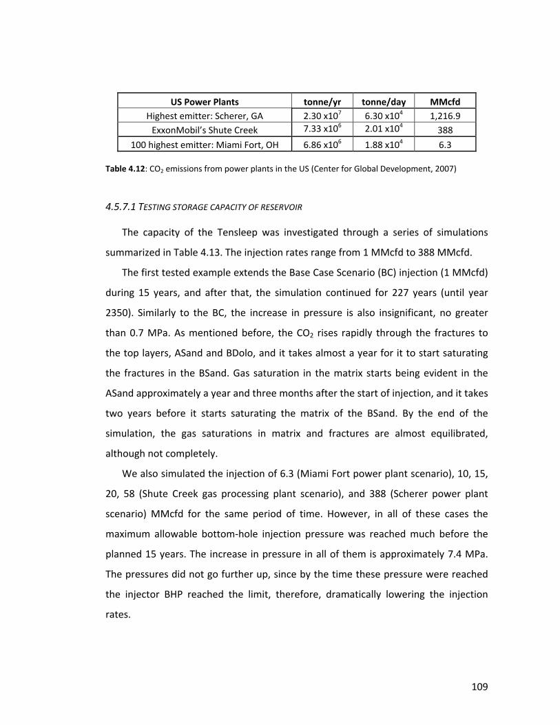
109
US Power Plants tonne/yr tonne/day MMcfd Highest emitter: Scherer, GA 2.30 x10⁷ 6.30 x10⁴ 1,216.9 ExxonMobil’s Shute Creek 7.33 x10⁶ 2.01 x10⁴ 388
100 highest emitter: Miami Fort, OH 6.86 x10⁶ 1.88 x10⁴ 6.3 Table 4.12: CO2 emissions from power plants in the US (Center for Global Development, 2007)
4.5.7.1 TESTING STORAGE CAPACITY OF RESERVOIR
The capacity of the Tensleep was investigated through a series of simulations
summarized in Table 4.13. The injection rates range from 1 MMcfd to 388 MMcfd.
The first tested example extends the Base Case Scenario (BC) injection (1 MMcfd)
during 15 years, and after that, the simulation continued for 227 years (until year
2350). Similarly to the BC, the increase in pressure is also insignificant, no greater
than 0.7 MPa. As mentioned before, the CO2 rises rapidly through the fractures to
the top layers, ASand and BDolo, and it takes almost a year for it to start saturating
the fractures in the BSand. Gas saturation in the matrix starts being evident in the
ASand approximately a year and three months after the start of injection, and it takes
two years before it starts saturating the matrix of the BSand. By the end of the
simulation, the gas saturations in matrix and fractures are almost equilibrated,
although not completely.
We also simulated the injection of 6.3 (Miami Fort power plant scenario), 10, 15,
20, 58 (Shute Creek gas processing plant scenario), and 388 (Scherer power plant
scenario) MMcfd for the same period of time. However, in all of these cases the
maximum allowable bottom‐hole injection pressure was reached much before the
planned 15 years. The increase in pressure in all of them is approximately 7.4 MPa.
The pressures did not go further up, since by the time these pressure were reached
the injector BHP reached the limit, therefore, dramatically lowering the injection
rates.
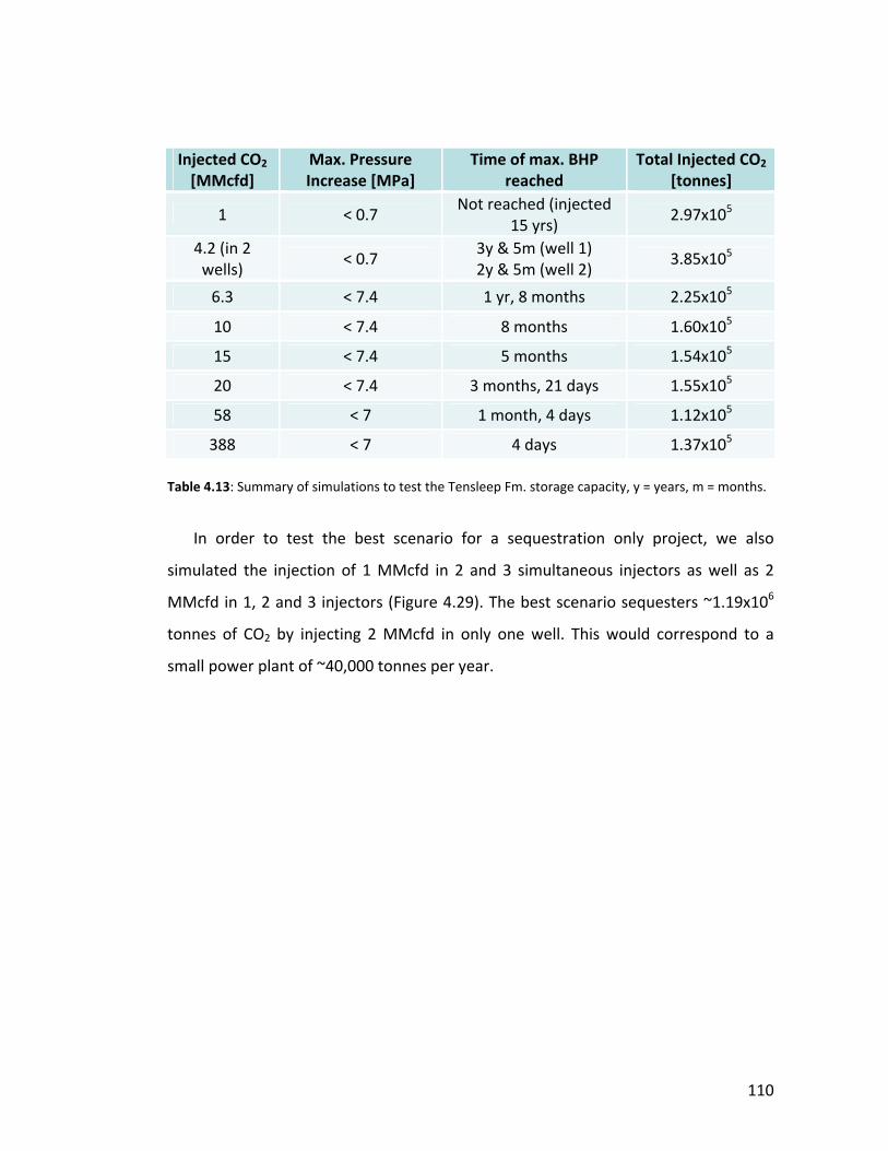
110
Injected CO2
[MMcfd] Max. Pressure Increase [MPa]
Time of max. BHP reached
Total Injected CO2 [tonnes]
1 < 0.7 Not reached (injected
15 yrs) 2.97x10⁵
4.2 (in 2 wells)
< 0.7 3y & 5m (well 1) 2y & 5m (well 2)
3.85x10⁵
6.3 < 7.4 1 yr, 8 months 2.25x10⁵
10 < 7.4 8 months 1.60x10⁵
15 < 7.4 5 months 1.54x10⁵
20 < 7.4 3 months, 21 days 1.55x10⁵
58 < 7 1 month, 4 days 1.12x10⁵
388 < 7 4 days 1.37x10⁵ Table 4.13: Summary of simulations to test the Tensleep Fm. storage capacity, y = years, m = months.
In order to test the best scenario for a sequestration only project, we also
simulated the injection of 1 MMcfd in 2 and 3 simultaneous injectors as well as 2
MMcfd in 1, 2 and 3 injectors (Figure 4.29). The best scenario sequesters ~1.19x10⁶
tonnes of CO2 by injecting 2 MMcfd in only one well. This would correspond to a
small power plant of ~40,000 tonnes per year.
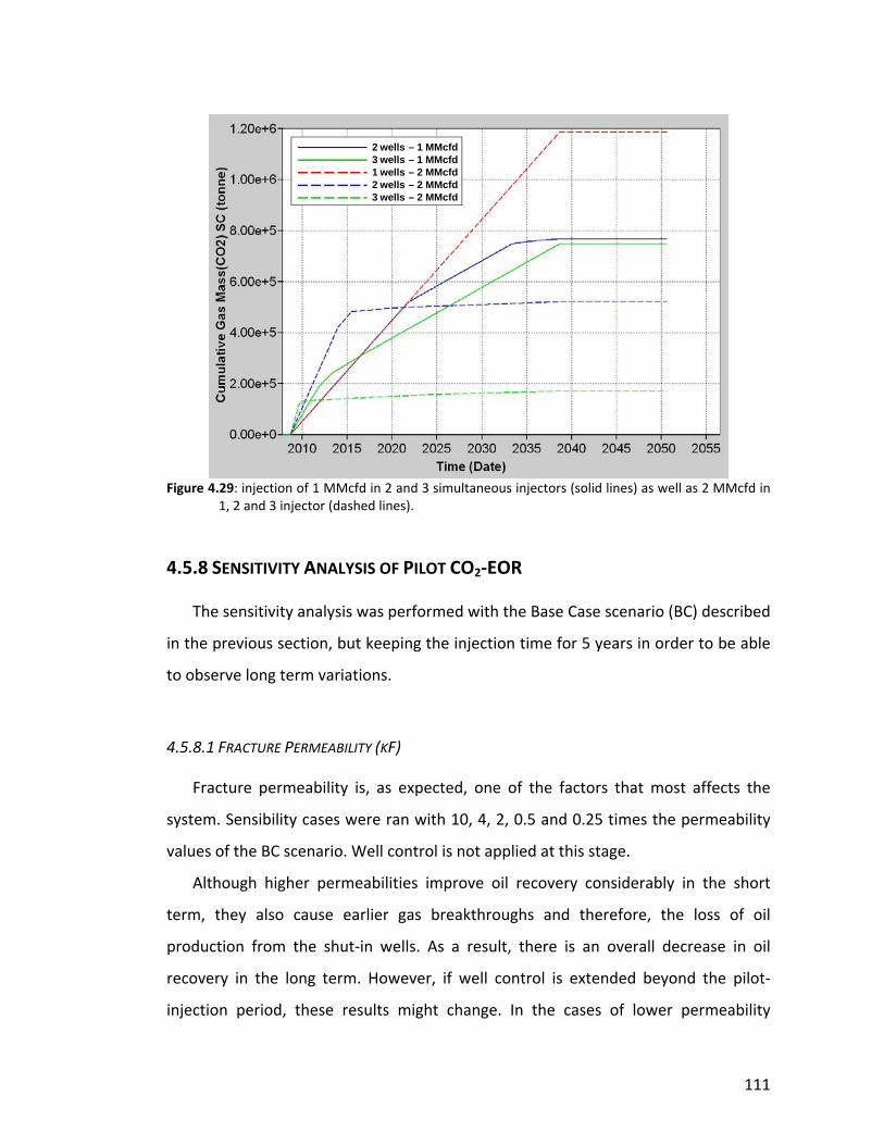
111
Figure 4.29: injection of 1 MMcfd in 2 and 3 simultaneous injectors (solid lines) as well as 2 MMcfd in 1, 2 and 3 injector (dashed lines).
4.5.8 SENSITIVITY ANALYSIS OF PILOT CO2‐EOR
The sensitivity analysis was performed with the Base Case scenario (BC) described
in the previous section, but keeping the injection time for 5 years in order to be able
to observe long term variations.
4.5.8.1 FRACTURE PERMEABILITY (KF)
Fracture permeability is, as expected, one of the factors that most affects the
system. Sensibility cases were ran with 10, 4, 2, 0.5 and 0.25 times the permeability
values of the BC scenario. Well control is not applied at this stage.
Although higher permeabilities improve oil recovery considerably in the short
term, they also cause earlier gas breakthroughs and therefore, the loss of oil
production from the shut‐in wells. As a result, there is an overall decrease in oil
recovery in the long term. However, if well control is extended beyond the pilot‐
injection period, these results might change. In the cases of lower permeability
2 wells – 1 MMcfd3 wells – 1 MMcfd1 wells – 2 MMcfd2 wells – 2 MMcfd3 wells – 2 MMcfd
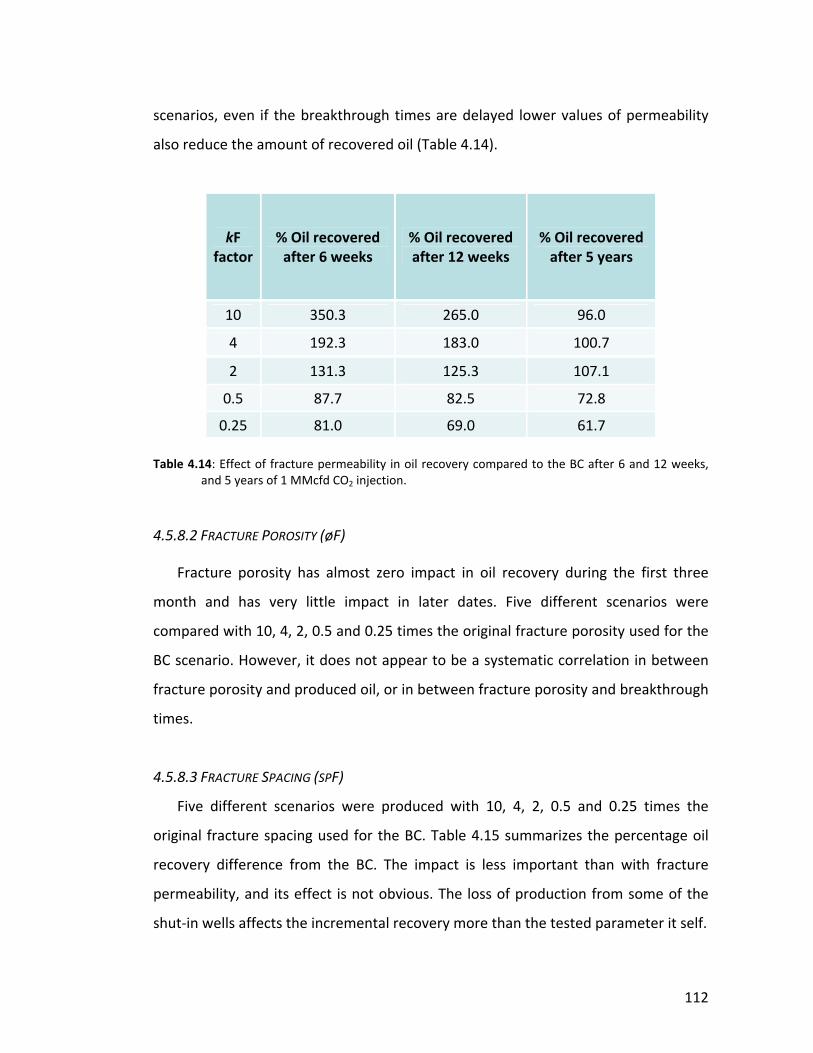
112
scenarios, even if the breakthrough times are delayed lower values of permeability
also reduce the amount of recovered oil (Table 4.14).
kF factor
% Oil recovered after 6 weeks
% Oil recovered after 12 weeks
% Oil recovered after 5 years
10 350.3 265.0 96.0
4 192.3 183.0 100.7
2 131.3 125.3 107.1
0.5 87.7 82.5 72.8
0.25 81.0 69.0 61.7 Table 4.14: Effect of fracture permeability in oil recovery compared to the BC after 6 and 12 weeks,
and 5 years of 1 MMcfd CO2 injection.
4.5.8.2 FRACTURE POROSITY (øF)
Fracture porosity has almost zero impact in oil recovery during the first three
month and has very little impact in later dates. Five different scenarios were
compared with 10, 4, 2, 0.5 and 0.25 times the original fracture porosity used for the
BC scenario. However, it does not appear to be a systematic correlation in between
fracture porosity and produced oil, or in between fracture porosity and breakthrough
times.
4.5.8.3 FRACTURE SPACING (SPF)
Five different scenarios were produced with 10, 4, 2, 0.5 and 0.25 times the
original fracture spacing used for the BC. Table 4.15 summarizes the percentage oil
recovery difference from the BC. The impact is less important than with fracture
permeability, and its effect is not obvious. The loss of production from some of the
shut‐in wells affects the incremental recovery more than the tested parameter it self.

113
spF factor
% Oil recovered after 6 weeks
% Oil recovered after 12 weeks
% Oil recovered after 5 years
10 125.1 132.2 102.0 4 106.2 112.3 112.0
2 101.0 103.5 102.8 0.5 100.5 100.0 102.2 0.25 103.1 99.1 96.4
Table 4.15: Effect of fracture spacing on oil recovered compared to the BC after 6 and 12 weeks, and 5
years of 1 MMcfd CO2 injection.
4.5.8.4 RELATIVE PERMEABILITY CURVES (KREL)
Four scenarios were created to test the effect of the relative permeability curves
in the model compared to the BC. In the base case scenario we use the same Krel for
the matrix than the one used in the history matching process while the fracture Krel
have the same saturations than the matrix, but with the typical X shape of fracture
Krel. The sensitivity scenarios include:
1. Fracture Krel of BC is used for both the matrix and the fracture system.
2. Matrix Krel is used for both matrix and fractures, as it was the case during the
history matching process (Figure 4.11).
3. Same matrix Krel than in the BC and X shaped fracture Krel with 0 initial water
saturation.
4. Average Krel curves described by Gaviria (2005) (Figure 4.30).
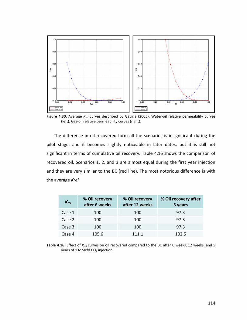
114
Figure 4.30: Average Krel curves described by Gaviria (2005). Water‐oil relative permeability curves (left); Gas‐oil relative permeability curves (right).
The difference in oil recovered form all the scenarios is insignificant during the
pilot stage, and it becomes slightly noticeable in later dates; but it is still not
significant in terms of cumulative oil recovery. Table 4.16 shows the comparison of
recovered oil. Scenarios 1, 2, and 3 are almost equal during the first year injection
and they are very similar to the BC (red line). The most notorious difference is with
the average Krel.
Krel % Oil recovery after 6 weeks
% Oil recovery after 12 weeks
% Oil recovery after 5 years
Case 1 100 100 97.3
Case 2 100 100 97.3
Case 3 100 100 97.3
Case 4 105.6 111.1 102.5 Table 4.16: Effect of Krel curves on oil recovered compared to the BC after 6 weeks, 12 weeks, and 5
years of 1 MMcfd CO2 injection.

115
4.5.8.5 MATRIX POROSITY & PERMEABILITY
Several scenarios were tested with different distributions of porosity and
permeability. In all of them there was little variation during the initial stages of
injection in the amount of oil recovered. Figure 4.31 shows and example of it, where
after the first month the results start varying due to the different timing of gas
breakthrough.
Figure 4.31: Oil rate comparison between BC (red line) and a case run with a different matrix porosity and permeability distribution.
4.5.8.5 GRID SIZE
As with the other tested parameters, grid size changes the CO2 breakthrough
times in different wells, complicating the possibility to make any valid quantitative
observations on how this refinements influence the system. For example, in the case
in which the grid was refined horizontally (I and J directions) by a factor of three, it is
possible to observe an increment in oil rates at the beginning of the injection.
Cumulative oil after 6 weeks of injection was 167.2% of the BC cumulative oil, while
116
in 12 weeks of injection it was 129.8%. However, breakthrough times diminished,
causing the closure of wells sooner than in the BC, and after 5 years of injection the
cumulative oil was 80.7% of the BC one.
However, it was clear from the simulations that in order to be able to resolve the
CO2 plume geometry we need a more refined grid both vertically and horizontally.
4.5.9 SENSITIVITY ANALYSIS OF PILOT CO2‐EOR WITHOUT GAS CONSTRAINTS
From the sensitivity analysis described in the previous section, it is extremely
difficult to drive any conclusion because the tested parameters greatly affect gas
breakthrough times, which also affects the resultant oil production and complicates
the direct comparison among scenarios. The imposed constraint in a well is to shut‐in
when gas rate is higher than 5000 cfd. Therefore, when the first well shuts‐in at
different times in each scenario, the distribution of the CO2 and the conditions of the
simulation change.
For these reasons, a different approach for the sensitivity analysis was taken; the
wells were allowed to produce without any gas production constraints. This permits
to analyze the effect of each tested parameter in the system. Nevertheless, the
resultant production is not the real production expected in the field and therefore,
this sensitivity analysis does not provide a range of possible outcomes regarding oil
production and CO2 storage.
The sensitivity simulations described in the previous sections were re‐run under
these new conditions.
Among all the parameters tested, fracture permeability is, as expected, one of
the factors that greater affects the system. Where in general, more oil is recovered
with higher fracture permeabilities (Figure 4.32). The other parameter that has a high
influence on the results is the relative permeability (Figure 4.33). On the other hand,
fracture spacing and specially fracture porosity are the factors that less influence
have on the results (Figures 4.34 and 4.35).
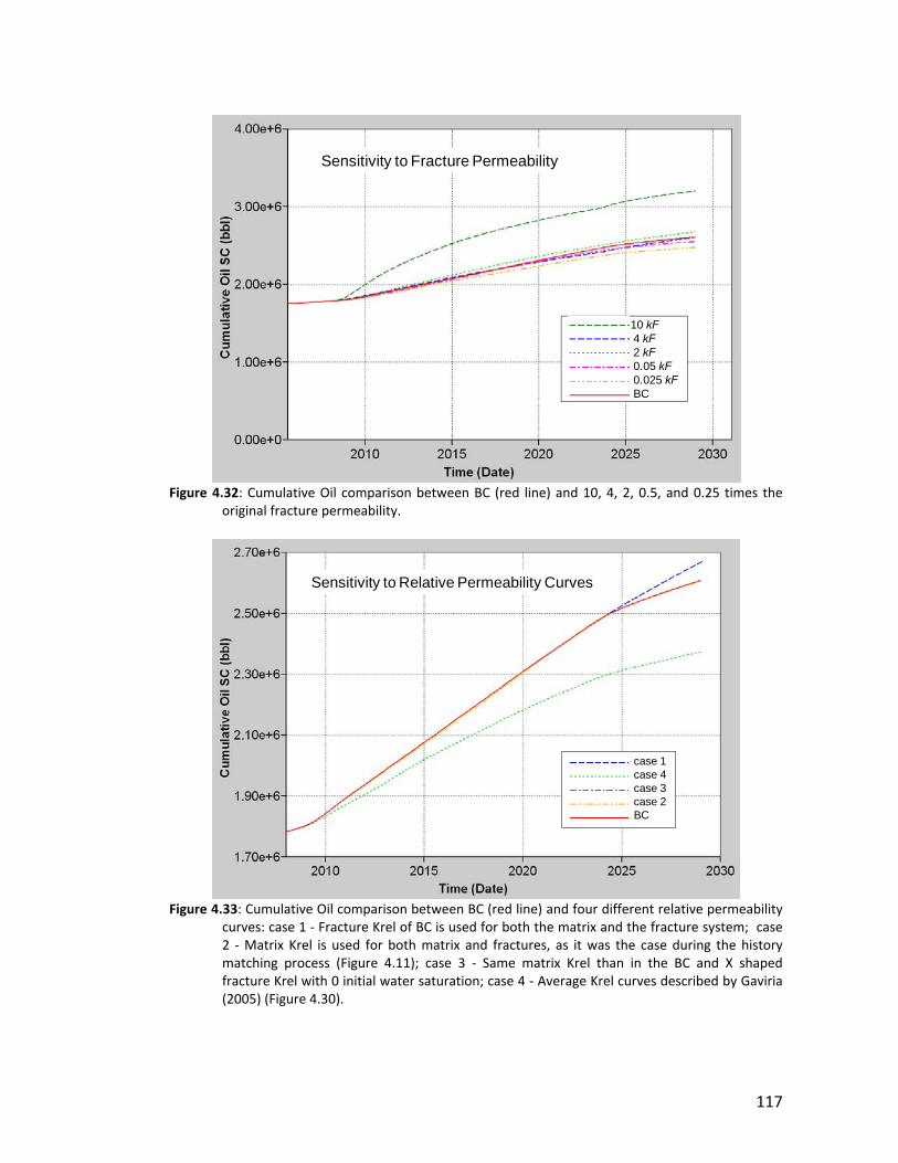
117
Figure 4.32: Cumulative Oil comparison between BC (red line) and 10, 4, 2, 0.5, and 0.25 times the original fracture permeability.
Figure 4.33: Cumulative Oil comparison between BC (red line) and four different relative permeability curves: case 1 ‐ Fracture Krel of BC is used for both the matrix and the fracture system; case 2 ‐ Matrix Krel is used for both matrix and fractures, as it was the case during the history matching process (Figure 4.11); case 3 ‐ Same matrix Krel than in the BC and X shaped fracture Krel with 0 initial water saturation; case 4 ‐ Average Krel curves described by Gaviria (2005) (Figure 4.30).
10 kF4 kF2 kF0.05 kF0.025 kFBC
Sensitivity to Fracture Permeability
case 1case 4case 3case 2BC
Sensitivity to Relative Permeability Curves
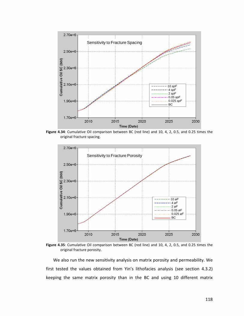
118
Figure 4.34: Cumulative Oil comparison between BC (red line) and 10, 4, 2, 0.5, and 0.25 times the original fracture spacing.
Figure 4.35: Cumulative Oil comparison between BC (red line) and 10, 4, 2, 0.5, and 0.25 times the original fracture porosity.
We also run the new sensitivity analysis on matrix porosity and permeability. We
first tested the values obtained from Yin’s lithofacies analysis (see section 4.3.2)
keeping the same matrix porosity than in the BC and using 10 different matrix
10 spF4 spF2 spF0.05 spF0.025 spFBC
Sensitivity to Fracture Spacing
10 øF4 øF2 øF0.05 øF0.025 øFBC
Sensitivity to Fracture Porosity
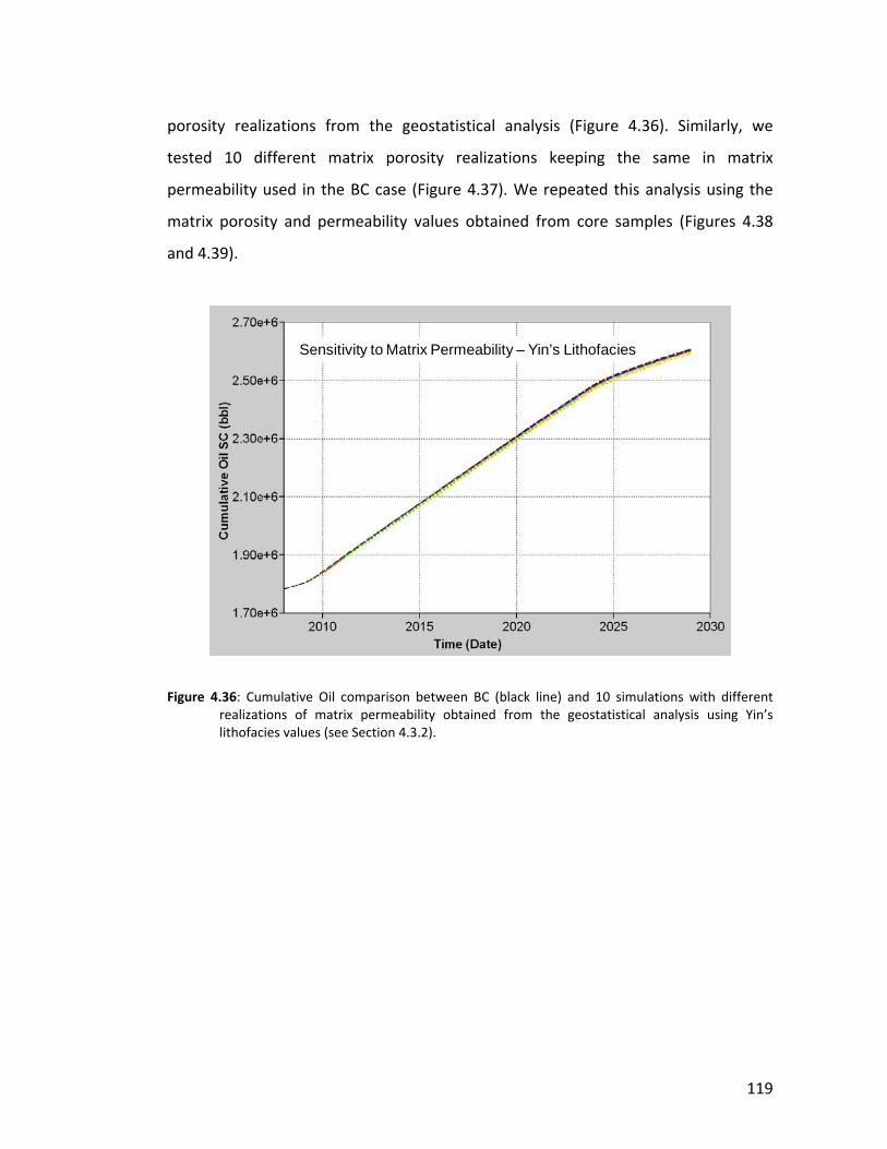
119
porosity realizations from the geostatistical analysis (Figure 4.36). Similarly, we
tested 10 different matrix porosity realizations keeping the same in matrix
permeability used in the BC case (Figure 4.37). We repeated this analysis using the
matrix porosity and permeability values obtained from core samples (Figures 4.38
and 4.39).
Figure 4.36: Cumulative Oil comparison between BC (black line) and 10 simulations with different realizations of matrix permeability obtained from the geostatistical analysis using Yin’s lithofacies values (see Section 4.3.2).
Sensitivity to Matrix Permeability – Yin’s Lithofacies
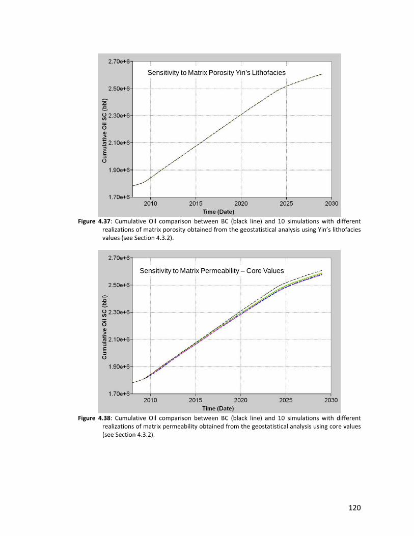
120
Figure 4.37: Cumulative Oil comparison between BC (black line) and 10 simulations with different realizations of matrix porosity obtained from the geostatistical analysis using Yin’s lithofacies values (see Section 4.3.2).
Figure 4.38: Cumulative Oil comparison between BC (black line) and 10 simulations with different realizations of matrix permeability obtained from the geostatistical analysis using core values (see Section 4.3.2).
Sensitivity to Matrix Porosity Yin’s Lithofacies
Sensitivity to Matrix Permeability – Core Values
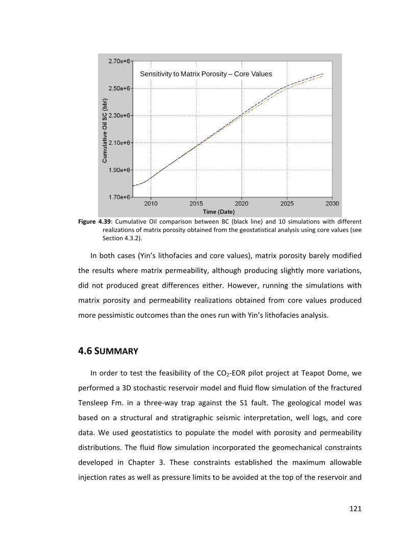
121
Figure 4.39: Cumulative Oil comparison between BC (black line) and 10 simulations with different realizations of matrix porosity obtained from the geostatistical analysis using core values (see Section 4.3.2).
In both cases (Yin’s lithofacies and core values), matrix porosity barely modified
the results where matrix permeability, although producing slightly more variations,
did not produced great differences either. However, running the simulations with
matrix porosity and permeability realizations obtained from core values produced
more pessimistic outcomes than the ones run with Yin’s lithofacies analysis.
4.6 SUMMARY
In order to test the feasibility of the CO2‐EOR pilot project at Teapot Dome, we
performed a 3D stochastic reservoir model and fluid flow simulation of the fractured
Tensleep Fm. in a three‐way trap against the S1 fault. The geological model was
based on a structural and stratigraphic seismic interpretation, well logs, and core
data. We used geostatistics to populate the model with porosity and permeability
distributions. The fluid flow simulation incorporated the geomechanical constraints
developed in Chapter 3. These constraints established the maximum allowable
injection rates as well as pressure limits to be avoided at the top of the reservoir and
Sensitivity to Matrix Porosity – Core Values
122
at the fault boundary. Similarly, we also incorporated a fracture permeability
anisotropy subparallel to the SHmax direction. We history matched our model with
historic oil and water rates from the field.
The results of the fluid flow simulation showed that the pressure increase is
minimal during the pilot project not constituting a risk for fault stability or seal
integrity. However, buoyancy and mobility of CO2 could represent a problem for the
EOR performance. CO2 was injected in the main producing interval (BSand) to
dissolve in the oil, but almost immediately rose to the top layers through the high
permeability fracture network, taking almost a year to start saturating the fractures
in the BSand. The mobility of the gas results in early breakthroughs in the closer wells
with their consequent shut‐in and loss of production.
Four different scenarios were tested as potential schemes for the projected CO2‐
EOR pilot, which consisted on the injection of: 1) 1 MMcfd for 6 weeks, 2) 1 MMcfd
for 12 weeks, 3) 2 MMcfd for 6 weeks and 4) 2 MMcfd for 12 weeks. In all of them, oil
recovery was less than the predicted from a pure primary production scenario due to
the mentioned closure of wells with high GOR. However, when a well control strategy
(re‐opening wells after a certain period of time) was implemented, incremental oil
recovery went up from 8%, in case 1, to 28%, in case 4, of the BC production.
The amount of CO2 planned to be injected in the initial pilot project is modest in
the context of making an impact in sequestering carbon dioxide. The storage
potential of the Tensleep was tested injecting higher amounts of CO2, which are
comparable to daily emissions of different size power plants. The results suggest that
the present trap could eventually hold an injection scheme of 2 MMcfd in a single
well during at least 30 years, sequestering ~1.2x10⁶ tonnes of CO2 corresponding to a
small power plant of ~40,000 tonnes per year. Due to the small size of the trap, there
seems not to be any advantage on injecting in multiple wells at the same time.
During the sensitivity analysis, we studied the impact on the system of several
parameters that included fracture permeability, porosity and spacing, relative
permeability curves, matrix porosity and permeability, and grid size. The results
123
suggested that several factors would influence the performance of a CO2 injection.
However, it is extremely difficult to drive any conclusion from this sensitivity analysis
because these parameters greatly affect gas breakthrough times (the imposed
constraint in a well is to shut it in when gas rate is higher than 5000 cfd). Therefore,
when the first well shuts‐in at different times in each scenario, the distribution of the
CO2 and the conditions of the simulation change, making the quantitative sensitivity
analysis meaningless.
A different approach for the sensitivity analysis was also taken, where the wells
were allowed to produce without any gas production constraints. This allowed us to
analyze the effect of these parameters in the system. But, since these are not the
real production conditions on the field, this approach would not provide a range of
possible outcomes regarding oil production and CO2 storage. Qualitatively, it was
observed that fracture permeability is the parameter that most influenced the CO2
and oil behavior where, Krel curves also have an important impact on the results.
Conversely, fracture porosity, fracture spacing, matrix porosity and matrix
permeability, seemed to have much less influence.
124
CHAPTER 5
FRACTURE DETECTION USING
AMPLITUDE VERSUS ANGLE AND
AZIMUTH AT TEAPOT DOME OIL
FIELD, WY
5.1 ABSTRACT
In this chapter we describe an Amplitude Versus Angle and Azimuth (AVAZ)
analysis performed at Teapot Dome to identify the presence of fractures using wide‐
azimuth 3D seismic data. The objective of the present analysis is to expand the 1D
scattered fracture characterization previously performed, to a 3D characterization of
the fracture network on both the reservoir and the caprock that will allow for a more
125
accurate assessment of the impact of these fractures in reservoir permeability and in
the risk of CO2 leakage.
In previous stages of this project, geomechanical analysis demonstrated that CO2
sequestration will neither induce slip on the reservoir‐bounding fault, nor fracture
the caprock. However, various sets of pre‐existing minor faults in the reservoir are
critically stressed (i.e., active) in the current stress field. Hence, raising pore pressure
during sequestration will activate slip on these minor faults. The presence of these
minor faults enhances formation permeability and injectivity of CO2. However, the
potential for slip on these faults could potentially compromise the top seal capacity
of the Tensleep if these minor faults extend up into the cap rock.
The AVAZ analysis uses amplitude variations in the long shot/receiver offsets of P‐
wave seismic data, to determine the orientation and magnitude of the seismic
anisotropy that could be correlated with the orientation and intensity of fractures.
The AVAZ results are calibrated with fracture intensity and orientations obtained
from FMI logs recorded in the area, as well as stress orientation, the macro fault
network of the anticline and the macro sedimentary structures. During the analysis of
these results, we did not found enough evidence to indicate whether the anisotropy
in the reservoir and caprock is influenced by stress, structural or sedimentary
features.
5.2 INTRODUCTION – MOTIVATION
As discussed in Chapters 2 and 3, the Tensleep Fm. is an eolian sandstone highly
fractured, where various sets of pre‐existing minor faults in the reservoir, and fewer
in the caprock, were found to be critically‐stressed (i.e., active) in the current stress
field.
The occurrence of these small faults in the caprock and the potential for slip on
these features could potentially compromise the top seal capacity of the Tensleep.
Similarly, the presence of these minor faults enhances formation permeability and
126
injectivity of CO2 in the reservoir. However, the fluid flow simulations discussed in
Chapter 4 showed that these fractures could provide conduits for the buoyant CO2 to
rapidly migrate to the top layers, away from the main producing interval, where the
CO2 was expected to dissolve into the oil to enhance its recovery. For this reason, it
will be extremely important to be able to discriminate areas in the reservoir with
higher fracture density from areas with lower fracture density in order to design
spatially more efficient CO2 injection schemes.
Traditional methods of fracture characterization are 1D (well logs or cores) or 2D
(outcrop analogs), but we need a technique that will allow us to spatially characterize
these features to better asses their contribution to reservoir permeability and the
potential risk of CO2 leakage in the caprock. These faults are below the resolution
limit of conventional 3D seismic imaging methods; yet, they are usually aligned in
sets that create anisotropy in seismic velocities (and permeabilities). Therefore, with
a 3D seismic cube it is possible to map seismic anisotropy and its spatial variability,
and obtain information on direction and density of these fractures (Gray and Head,
2000; Hall et al., 2002; Gray, 2008).
In this chapter we describe the study we conducted using Amplitude Versus Angle
and Azimuth (AVAZ) analysis to identify the presence of fractures in the reservoir and
caprock based on wide‐azimuth 3D seismic data, which is based on azimuthal
anisotropy measurements.
5.3 SEISMIC ANISOTROPY
Seismic anisotropy has been recognized as a widespread phenomenon in the
upper crust and even in the upper mantle. There are several causes for this effective
seismic anisotropy, but in the crystalline upper crust it can be related to two main
mechanisms: stress‐related anisotropy and structural anisotropy (Boness, 2005).
Stress‐related anisotropy is the response to an anisotropic tectonic stress. The
mechanisms proposed to cause this effect are the preferential closure of fractures,
127
perpendicular to the maximum horizontal compressive stress (SHmax) in a randomly
fractured crust (Boness and Zoback, 2004); or the presence of SHmax aligned liquid‐
filled microcracks (Crampin, 1985). In both cases, a seismic wave propagating in the
vertical plane will be polarized with a fast direction parallel to SHmax (Bonnes, 2005).
Structural anisotropy will be the result of aligned parallel macroscopic fractures and
faults, parallel sedimentary planes and the alignment of minerals and/or grains. Here
the fast polarization direction will be parallel to the strike of the structural fabric
(Boness, 2005).
Traditional analyses of crustal anisotropy are based on shear waves (shear‐wave
splitting analysis). When a shear‐wave enters a zone of effective seismic anisotropy,
it splits into two or more phases with different velocities and polarizations. The
polarization is controlled by the three dimensional symmetry of the anisotropy, and
the delay between them is proportional to the differential slowness of the shear
wave in the direction of the ray path and the length of the path through the
anisotropic material (Crampin, 1984).
A very common cause of seismic anisotropy is the presence of fractures.
Therefore, several methods have been developed for fracture characterization in
reservoirs. The goal of this analysis is to obtain Thomsen’s coefficient γ, which is the
fractional difference between velocities of split shear waves at vertical incidence. γ is
related to crack density, which is also related to the permeability of the fracture
network, and it can be obtained from the difference in shear‐wave travel times and
normal‐incident reflection amplitudes. However, this methodology is difficult to
implement at a reservoir scale because high‐quality shear data could be very difficult
and expensive to obtain (Rüger and Tsvankin, 1997).
The influence of azimuthal anisotropy on P‐wave propagation is not as dramatic
as for shear waves, but it still can be considerable. It has been demonstrated that
fracturing causes significant azimuthal variation in recorded seismic signatures, and
since traditional seismic exploration data is much more common and available, the
128
characterization of fractured reservoirs using surface seismic data became an
increasingly important exploration problem (Rüger and Tsvankin, 1997).
Rüger and Tsvankin (1997) showed the Amplitude‐variation‐with‐offset (AVO)
response of fractures reservoirs. AVO analysis consists in extracting reflection
coefficients (ratio of amplitudes of reflected and incident seismic waves) from
seismic data, and interpreting it in terms of the change in medium parameters. They
illustrated that P‐wave amplitudes could be sensitive even to relatively weak
anisotropy of the rock, and they showed how the azimuthally dependent AVO
signature can be interpreted and combined with normal‐moveout and shear‐wave‐
splitting analyses (if available) to constrain the crack density and other medium
parameters.
5.4 AVAZ METHOD IN FRACTURED RESERVOIRS
The AVAZ analysis uses amplitude variations in the long shot/receiver offsets of P‐
wave seismic data to determine the intensity and orientation of fractures (Gray et al.,
2003). It is a sample‐by‐sample fitting of the amplitudes in the prestack seismic
gather to an equation derived by Rüger (1996):
R (i,φ) = A + [Biso + Bani cos2 (φ – φsym)]sin2 i
where R is the reflectivity (amplitude) of the P wave, A is the AVO intercept, Biso is the
isotropic AVO gradient, Bani is the anisotropic gradient (or crack density), i is the
incident angle of the seismic wave and φ is the azimuth of the ray path, and φsym is
the azimuth of the direction, perpendicular to the fracture strike. This equation
describes how the amplitude of reflected P‐wave on the interface between two
azimuthal anisotropic media varies at different incident angles and azimuths (Figure
5.1, left) of the ray path (Zheng et al. 2004).
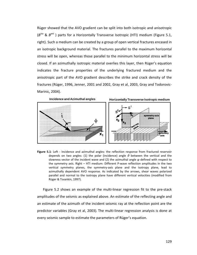
129
Rüger showed that the AVO gradient can be split into both isotropic and anisotropic
(Biso & Bani ) parts for a Horizontally Transverse Isotropic (HTI) medium (Figure 5.1,
right). Such a medium can be created by a group of open vertical fractures encased in
an isotropic background material. The fractures parallel to the maximum horizontal
stress will be open, whereas those parallel to the minimum horizontal stress will be
closed. If an azimuthally isotropic material overlies this layer, then Rüger’s equation
indicates the fracture properties of the underlying fractured medium and the
anisotropic part of the AVO gradient describes the strike and crack density of the
fractures (Rüger, 1996, Jenner, 2001 and 2002, Gray et al, 2003, Gray and Todorovic‐
Marinic, 2004).
Figure 5.1: Left ‐ Incidence and azimuthal angles: the reflection response from fractured reservoir
depends on two angles: (1) the polar (incidence) angle θ between the vertical and the slowness vector of the incident wave and (2) the azimuthal angle φ defined with respect to the symmetry axis. Right – HTI medium: Different P‐wave reflection amplitudes in the two vertical symmetry planes, the symmetry‐axis plane and the isotropy plane, lead to azimuthally dependent AVO response. As indicated by the arrows, shear waves polarized parallel and normal to the isotropy plane have different vertical velocities (modified from Rüger & Tsvankin, 1997).
Figure 5.2 shows an example of the multi‐linear regression fit to the pre‐stack
amplitudes of the seismic as explained above. An estimate of the reflecting angle and
an estimate of the azimuth of the incident seismic ray at the reflection point are the
predictor variables (Gray et al, 2003). The multi‐linear regression analysis is done at
every seismic sample to estimate the parameters of Rüger’s equation.
Incidence and Azimuthal angles Horizontally Transverse Isotropic medium
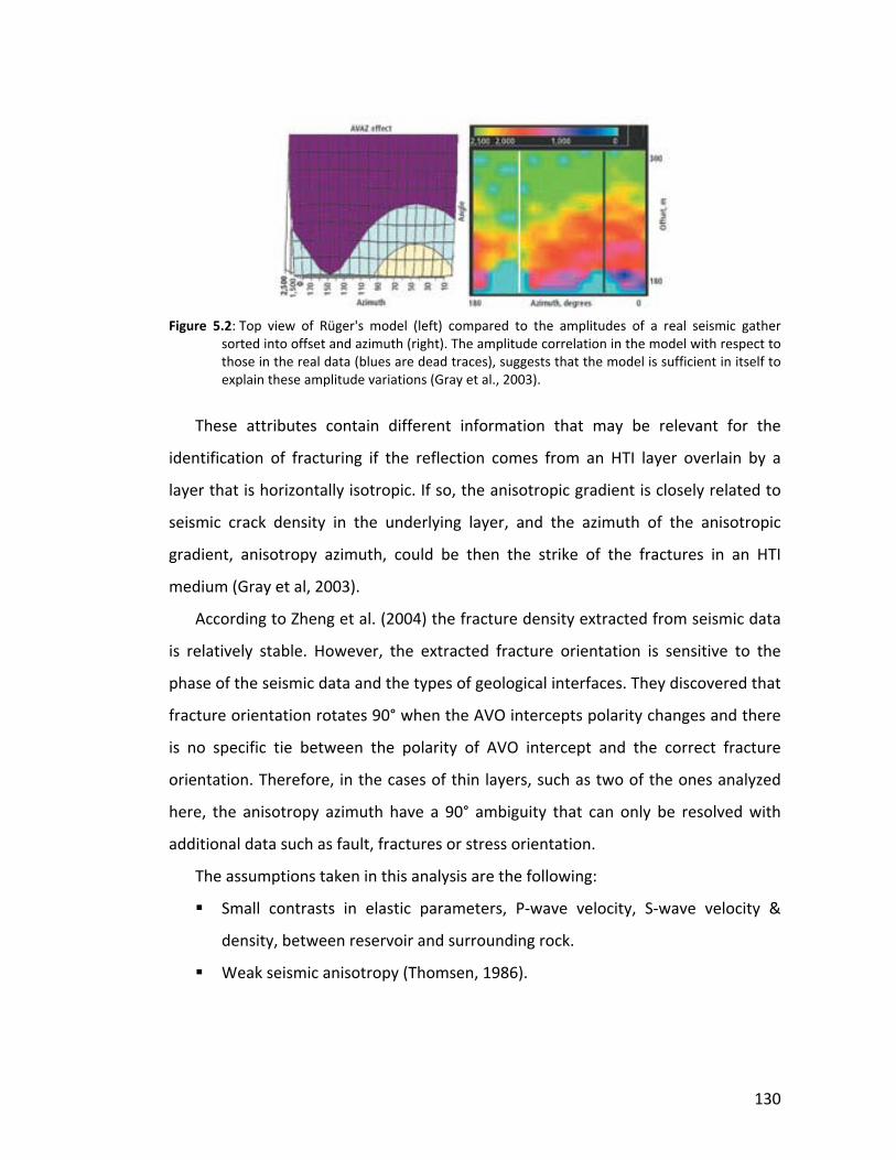
130
Figure 5.2: Top view of Rüger's model (left) compared to the amplitudes of a real seismic gather sorted into offset and azimuth (right). The amplitude correlation in the model with respect to those in the real data (blues are dead traces), suggests that the model is sufficient in itself to explain these amplitude variations (Gray et al., 2003).
These attributes contain different information that may be relevant for the
identification of fracturing if the reflection comes from an HTI layer overlain by a
layer that is horizontally isotropic. If so, the anisotropic gradient is closely related to
seismic crack density in the underlying layer, and the azimuth of the anisotropic
gradient, anisotropy azimuth, could be then the strike of the fractures in an HTI
medium (Gray et al, 2003).
According to Zheng et al. (2004) the fracture density extracted from seismic data
is relatively stable. However, the extracted fracture orientation is sensitive to the
phase of the seismic data and the types of geological interfaces. They discovered that
fracture orientation rotates 90° when the AVO intercepts polarity changes and there
is no specific tie between the polarity of AVO intercept and the correct fracture
orientation. Therefore, in the cases of thin layers, such as two of the ones analyzed
here, the anisotropy azimuth have a 90° ambiguity that can only be resolved with
additional data such as fault, fractures or stress orientation.
The assumptions taken in this analysis are the following:
Small contrasts in elastic parameters, P‐wave velocity, S‐wave velocity &
density, between reservoir and surrounding rock.
Weak seismic anisotropy (Thomsen, 1986).
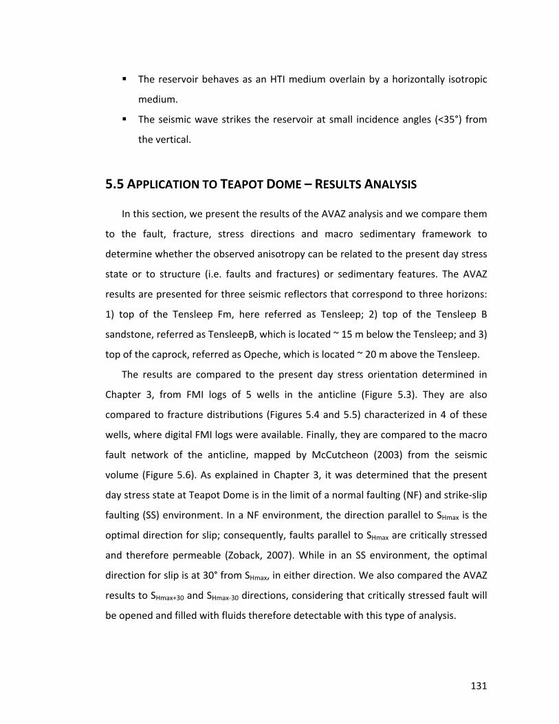
131
The reservoir behaves as an HTI medium overlain by a horizontally isotropic
medium.
The seismic wave strikes the reservoir at small incidence angles (<35°) from
the vertical.
5.5 APPLICATION TO TEAPOT DOME – RESULTS ANALYSIS
In this section, we present the results of the AVAZ analysis and we compare them
to the fault, fracture, stress directions and macro sedimentary framework to
determine whether the observed anisotropy can be related to the present day stress
state or to structure (i.e. faults and fractures) or sedimentary features. The AVAZ
results are presented for three seismic reflectors that correspond to three horizons:
1) top of the Tensleep Fm, here referred as Tensleep; 2) top of the Tensleep B
sandstone, referred as TensleepB, which is located ~ 15 m below the Tensleep; and 3)
top of the caprock, referred as Opeche, which is located ~ 20 m above the Tensleep.
The results are compared to the present day stress orientation determined in
Chapter 3, from FMI logs of 5 wells in the anticline (Figure 5.3). They are also
compared to fracture distributions (Figures 5.4 and 5.5) characterized in 4 of these
wells, where digital FMI logs were available. Finally, they are compared to the macro
fault network of the anticline, mapped by McCutcheon (2003) from the seismic
volume (Figure 5.6). As explained in Chapter 3, it was determined that the present
day stress state at Teapot Dome is in the limit of a normal faulting (NF) and strike‐slip
faulting (SS) environment. In a NF environment, the direction parallel to SHmax is the
optimal direction for slip; consequently, faults parallel to SHmax are critically stressed
and therefore permeable (Zoback, 2007). While in an SS environment, the optimal
direction for slip is at 30° from SHmax, in either direction. We also compared the AVAZ
results to SHmax+30 and SHmax‐30 directions, considering that critically stressed fault will
be opened and filled with fluids therefore detectable with this type of analysis.
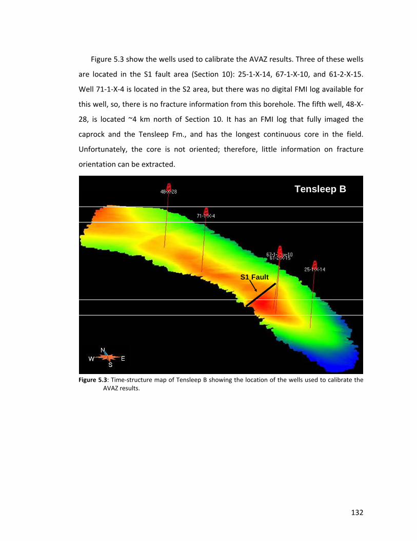
132
Figure 5.3 show the wells used to calibrate the AVAZ results. Three of these wells
are located in the S1 fault area (Section 10): 25‐1‐X‐14, 67‐1‐X‐10, and 61‐2‐X‐15.
Well 71‐1‐X‐4 is located in the S2 area, but there was no digital FMI log available for
this well, so, there is no fracture information from this borehole. The fifth well, 48‐X‐
28, is located ~4 km north of Section 10. It has an FMI log that fully imaged the
caprock and the Tensleep Fm., and has the longest continuous core in the field.
Unfortunately, the core is not oriented; therefore, little information on fracture
orientation can be extracted.
Figure 5.3: Time‐structure map of Tensleep B showing the location of the wells used to calibrate the AVAZ results.
S1 Fault
Tensleep B
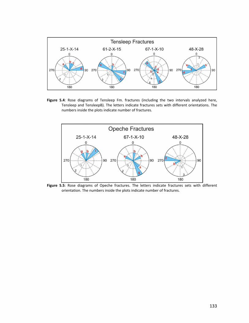
133
Figure 5.4: Rose diagrams of Tensleep Fm. fractures (including the two intervals analyzed here,
Tensleep and TensleepB). The letters indicate fractures sets with different orientations. The numbers inside the plots indicate number of fractures.
Figure 5.5: Rose diagrams of Opeche fractures. The letters indicate fractures sets with different orientation. The numbers inside the plots indicate number of fractures.
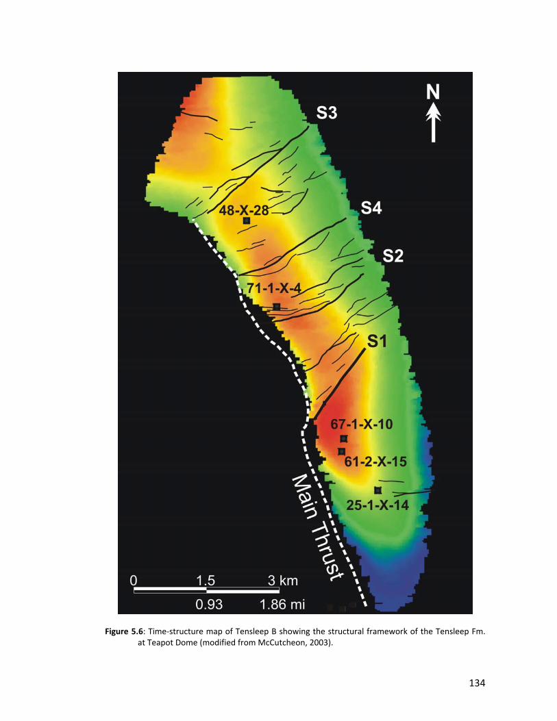
134
Figure 5.6: Time‐structure map of Tensleep B showing the structural framework of the Tensleep Fm.
at Teapot Dome (modified from McCutcheon, 2003).
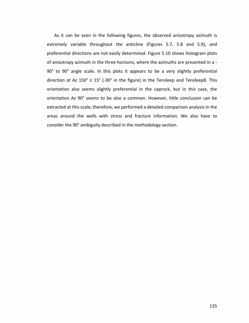
135
As it can be seen in the following figures, the observed anisotropy azimuth is
extremely variable throughout the anticline (Figures 5.7, 5.8 and 5.9), and
preferential directions are not easily determined. Figure 5.10 shows histogram plots
of anisotropy azimuth in the three horizons, where the azimuths are presented in a ‐
90° to 90° angle scale. In this plots it appears to be a very slightly preferential
direction at Az 150° ± 15° (‐30° in the figure) in the Tensleep and TensleepB. This
orientation also seems slightly preferential in the caprock, but in this case, the
orientation Az 90° seems to be also a common. However, little conclusion can be
extracted at this scale; therefore, we performed a detailed comparison analysis in the
areas around the wells with stress and fracture information. We also have to
consider the 90° ambiguity described in the methodology section.
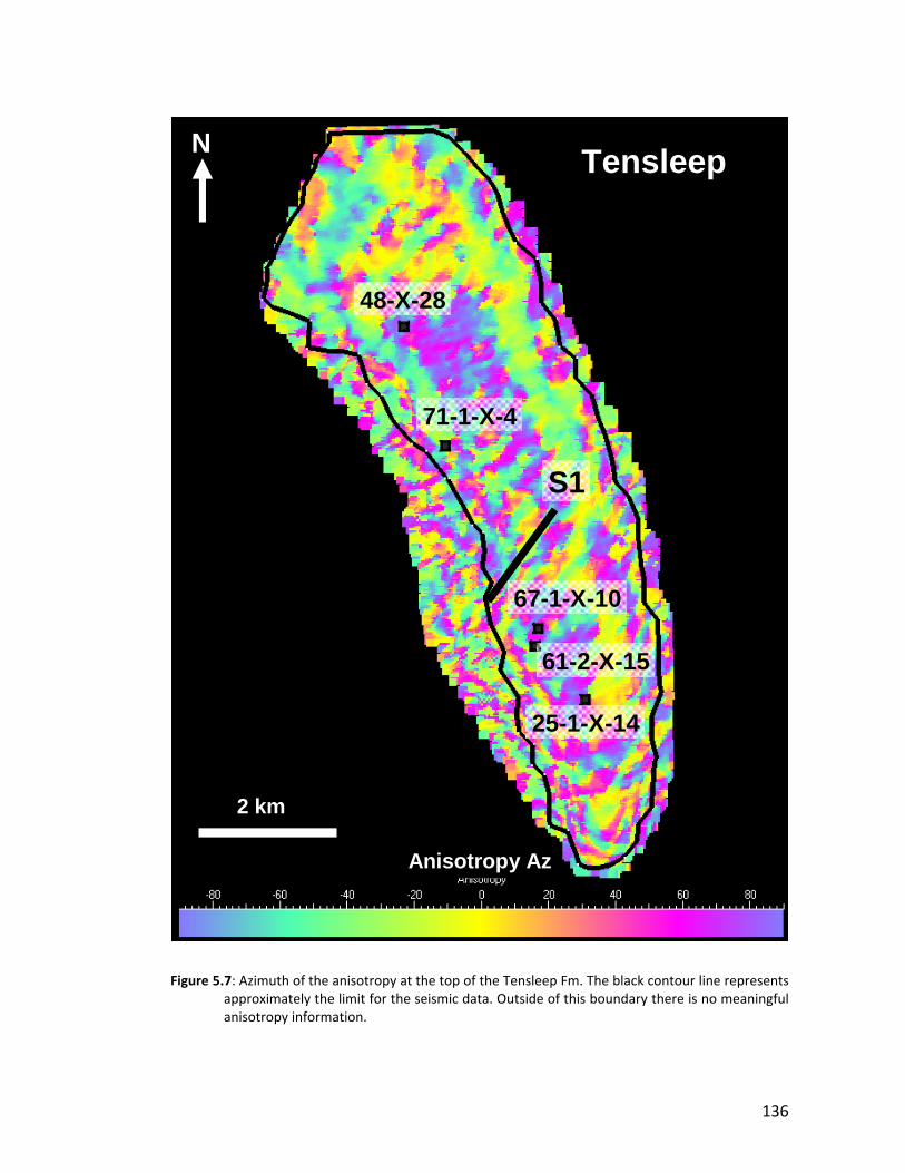
136
Figure 5.7: Azimuth of the anisotropy at the top of the Tensleep Fm. The black contour line represents
approximately the limit for the seismic data. Outside of this boundary there is no meaningful anisotropy information.
Tensleep
S1
48-X-28
71-1-X-4
67-1-X-10
61-2-X-15
25-1-X-14
Anisotropy Az
2 km
N
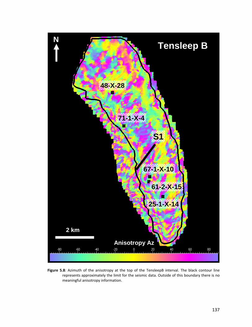
137
Figure 5.8: Azimuth of the anisotropy at the top of the TensleepB interval. The black contour line
represents approximately the limit for the seismic data. Outside of this boundary there is no meaningful anisotropy information.
Tensleep B
S1
48-X-28
71-1-X-4
67-1-X-10
61-2-X-15
25-1-X-14
Anisotropy Az
2 km
N
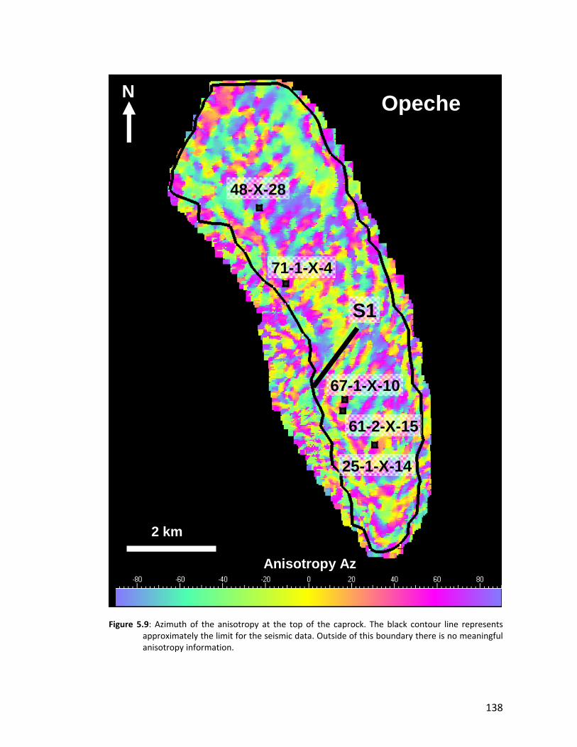
138
Figure 5.9: Azimuth of the anisotropy at the top of the caprock. The black contour line represents
approximately the limit for the seismic data. Outside of this boundary there is no meaningful anisotropy information.
Opeche
S1
48-X-28
71-1-X-4
67-1-X-10
61-2-X-15
25-1-X-14
Anisotropy Az
2 km
N
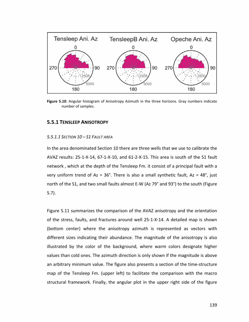
139
Figure 5.10: Angular histogram of Anisotropy Azimuth in the three horizons. Gray numbers indicate
number of samples.
5.5.1 TENSLEEP ANISOTROPY
5.5.1.1 SECTION 10 – S1 FAULT AREA
In the area denominated Section 10 there are three wells that we use to calibrate the
AVAZ results: 25‐1‐X‐14, 67‐1‐X‐10, and 61‐2‐X‐15. This area is south of the S1 fault
network , which at the depth of the Tensleep Fm. it consist of a principal fault with a
very uniform trend of Az = 36°. There is also a small synthetic fault, Az = 48°, just
north of the S1, and two small faults almost E‐W (Az 79° and 93°) to the south (Figure
5.7).
Figure 5.11 summarizes the comparison of the AVAZ anisotropy and the orientation
of the stress, faults, and fractures around well 25‐1‐X‐14. A detailed map is shown
(bottom center) where the anisotropy azimuth is represented as vectors with
different sizes indicating their abundance. The magnitude of the anisotropy is also
illustrated by the color of the background, where warm colors designate higher
values than cold ones. The azimuth direction is only shown if the magnitude is above
an arbitrary minimum value. The figure also presents a section of the time‐structure
map of the Tensleep Fm. (upper left) to facilitate the comparison with the macro
structural framework. Finally, the angular plot in the upper right side of the figure
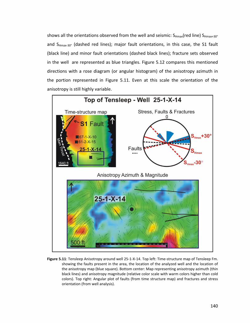
140
shows all the orientations observed from the well and seismic: SHmax(red line) SHmax+30°
and SHmax‐30° (dashed red lines); major fault orientations, in this case, the S1 fault
(black line) and minor fault orientations (dashed black lines); fracture sets observed
in the well are represented as blue triangles. Figure 5.12 compares this mentioned
directions with a rose diagram (or angular histogram) of the anisotropy azimuth in
the portion represented in Figure 5.11. Even at this scale the orientation of the
anisotropy is still highly variable.
Figure 5.11: Tensleep Anisotropy around well 25‐1‐X‐14. Top left: Time‐structure map of Tensleep Fm.
showing the faults present in the area, the location of the analyzed well and the location of the anisotropy map (blue square). Bottom center: Map representing anisotropy azimuth (thin black lines) and anisotropy magnitude (relative color scale with warm colors higher than cold colors). Top right: Angular plot of faults (from time structure map) and fractures and stress orientation (from well analysis).
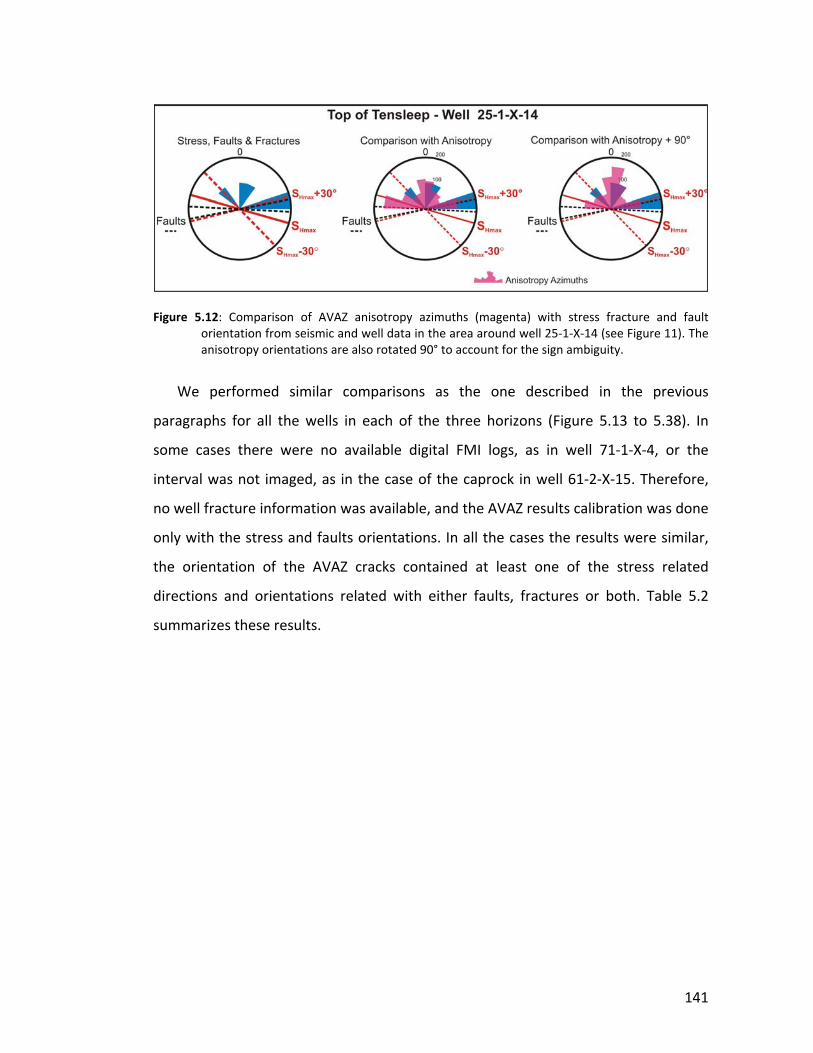
141
Figure 5.12: Comparison of AVAZ anisotropy azimuths (magenta) with stress fracture and fault
orientation from seismic and well data in the area around well 25‐1‐X‐14 (see Figure 11). The anisotropy orientations are also rotated 90° to account for the sign ambiguity.
We performed similar comparisons as the one described in the previous
paragraphs for all the wells in each of the three horizons (Figure 5.13 to 5.38). In
some cases there were no available digital FMI logs, as in well 71‐1‐X‐4, or the
interval was not imaged, as in the case of the caprock in well 61‐2‐X‐15. Therefore,
no well fracture information was available, and the AVAZ results calibration was done
only with the stress and faults orientations. In all the cases the results were similar,
the orientation of the AVAZ cracks contained at least one of the stress related
directions and orientations related with either faults, fractures or both. Table 5.2
summarizes these results.
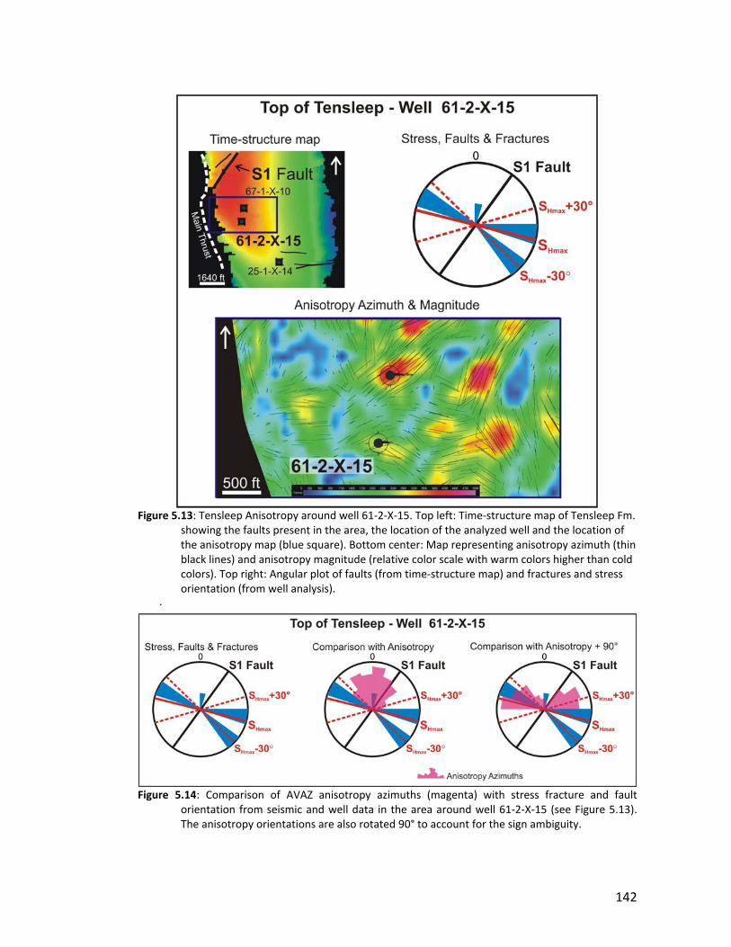
142
Figure 5.13: Tensleep Anisotropy around well 61‐2‐X‐15. Top left: Time‐structure map of Tensleep Fm. showing the faults present in the area, the location of the analyzed well and the location of the anisotropy map (blue square). Bottom center: Map representing anisotropy azimuth (thin black lines) and anisotropy magnitude (relative color scale with warm colors higher than cold colors). Top right: Angular plot of faults (from time‐structure map) and fractures and stress orientation (from well analysis).
.
Figure 5.14: Comparison of AVAZ anisotropy azimuths (magenta) with stress fracture and fault orientation from seismic and well data in the area around well 61‐2‐X‐15 (see Figure 5.13). The anisotropy orientations are also rotated 90° to account for the sign ambiguity.
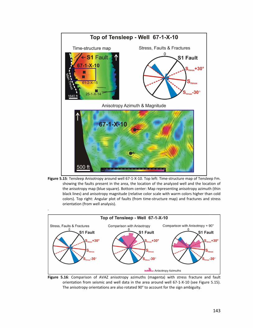
143
Figure 5.15: Tensleep Anisotropy around well 67‐1‐X‐10. Top left: Time‐structure map of Tensleep Fm. showing the faults present in the area, the location of the analyzed well and the location of the anisotropy map (blue square). Bottom center: Map representing anisotropy azimuth (thin black lines) and anisotropy magnitude (relative color scale with warm colors higher than cold colors). Top right: Angular plot of faults (from time‐structure map) and fractures and stress orientation (from well analysis).
.
Figure 5.16: Comparison of AVAZ anisotropy azimuths (magenta) with stress fracture and fault orientation from seismic and well data in the area around well 67‐1‐X‐10 (see Figure 5.15). The anisotropy orientations are also rotated 90° to account for the sign ambiguity.
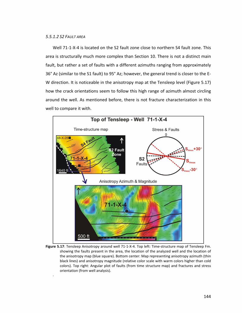
144
5.5.1.2 S2 FAULT AREA
Well 71‐1‐X‐4 is located on the S2 fault zone close to northern S4 fault zone. This
area is structurally much more complex than Section 10. There is not a distinct main
fault, but rather a set of faults with a different azimuths ranging from approximately
36° Az (similar to the S1 fault) to 95° Az; however, the general trend is closer to the E‐
W direction. It is noticeable in the anisotropy map at the Tensleep level (Figure 5.17)
how the crack orientations seem to follow this high range of azimuth almost circling
around the well. As mentioned before, there is not fracture characterization in this
well to compare it with.
Figure 5.17: Tensleep Anisotropy around well 71‐1‐X‐4. Top left: Time‐structure map of Tensleep Fm. showing the faults present in the area, the location of the analyzed well and the location of the anisotropy map (blue square). Bottom center: Map representing anisotropy azimuth (thin black lines) and anisotropy magnitude (relative color scale with warm colors higher than cold colors). Top right: Angular plot of faults (from time structure map) and fractures and stress orientation (from well analysis).
.
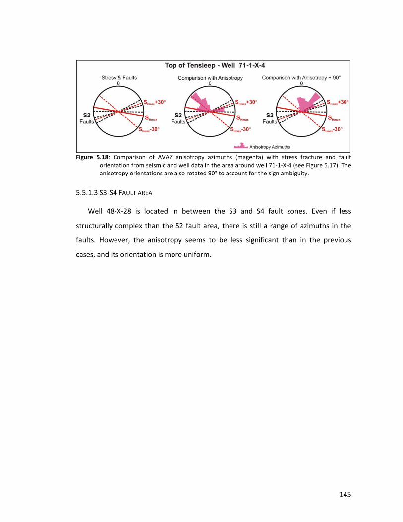
145
Figure 5.18: Comparison of AVAZ anisotropy azimuths (magenta) with stress fracture and fault orientation from seismic and well data in the area around well 71‐1‐X‐4 (see Figure 5.17). The anisotropy orientations are also rotated 90° to account for the sign ambiguity.
5.5.1.3 S3‐S4 FAULT AREA
Well 48‐X‐28 is located in between the S3 and S4 fault zones. Even if less
structurally complex than the S2 fault area, there is still a range of azimuths in the
faults. However, the anisotropy seems to be less significant than in the previous
cases, and its orientation is more uniform.

146
Figure 5.19: Tensleep Anisotropy around well 48‐X‐28. Top left Time‐structure map of Tensleep Fm. showing the faults present in the area, the location of the analyzed well and the location of the anisotropy map (blue square). Bottom center: Map representing anisotropy azimuth (thin black lines) and anisotropy magnitude (relative color scale with warm colors higher than cold colors). Top right: Angular plot of faults (from time‐structure map) and fractures and stress orientation (from well analysis).
Figure 5.20: Comparison of AVAZ anisotropy azimuths (magenta) with stress fracture and fault orientation from seismic and well data in the area around well 48‐X‐28 (see Figure 5.19). The anisotropy orientations are also rotated 90° to account for the sign ambiguity.
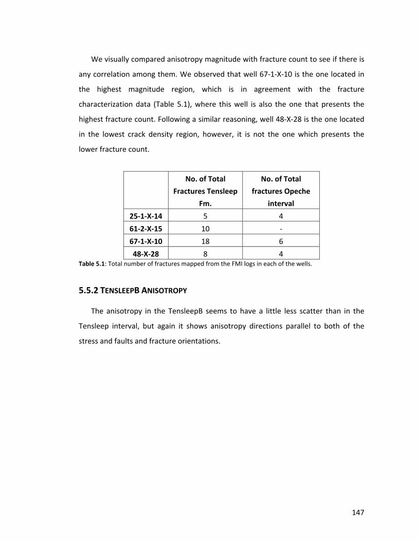
147
We visually compared anisotropy magnitude with fracture count to see if there is
any correlation among them. We observed that well 67‐1‐X‐10 is the one located in
the highest magnitude region, which is in agreement with the fracture
characterization data (Table 5.1), where this well is also the one that presents the
highest fracture count. Following a similar reasoning, well 48‐X‐28 is the one located
in the lowest crack density region, however, it is not the one which presents the
lower fracture count.
No. of Total
Fractures Tensleep
Fm.
No. of Total
fractures Opeche
interval
25‐1‐X‐14 5 4
61‐2‐X‐15 10 ‐
67‐1‐X‐10 18 6
48‐X‐28 8 4 Table 5.1: Total number of fractures mapped from the FMI logs in each of the wells.
5.5.2 TENSLEEPB ANISOTROPY
The anisotropy in the TensleepB seems to have a little less scatter than in the
Tensleep interval, but again it shows anisotropy directions parallel to both of the
stress and faults and fracture orientations.
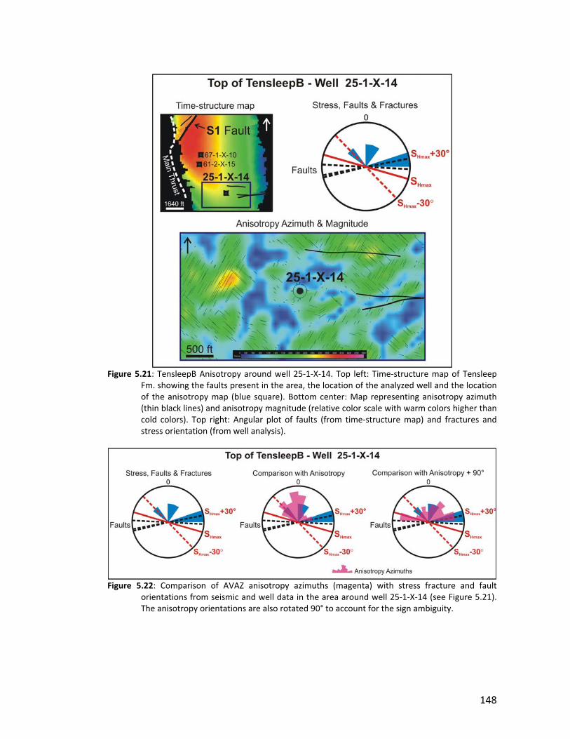
148
Figure 5.21: TensleepB Anisotropy around well 25‐1‐X‐14. Top left: Time‐structure map of Tensleep Fm. showing the faults present in the area, the location of the analyzed well and the location of the anisotropy map (blue square). Bottom center: Map representing anisotropy azimuth (thin black lines) and anisotropy magnitude (relative color scale with warm colors higher than cold colors). Top right: Angular plot of faults (from time‐structure map) and fractures and stress orientation (from well analysis).
Figure 5.22: Comparison of AVAZ anisotropy azimuths (magenta) with stress fracture and fault orientations from seismic and well data in the area around well 25‐1‐X‐14 (see Figure 5.21). The anisotropy orientations are also rotated 90° to account for the sign ambiguity.
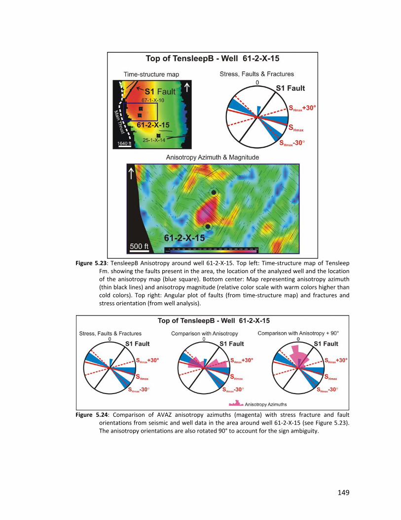
149
Figure 5.23: TensleepB Anisotropy around well 61‐2‐X‐15. Top left: Time‐structure map of Tensleep Fm. showing the faults present in the area, the location of the analyzed well and the location of the anisotropy map (blue square). Bottom center: Map representing anisotropy azimuth (thin black lines) and anisotropy magnitude (relative color scale with warm colors higher than cold colors). Top right: Angular plot of faults (from time‐structure map) and fractures and stress orientation (from well analysis).
Figure 5.24: Comparison of AVAZ anisotropy azimuths (magenta) with stress fracture and fault orientations from seismic and well data in the area around well 61‐2‐X‐15 (see Figure 5.23). The anisotropy orientations are also rotated 90° to account for the sign ambiguity.
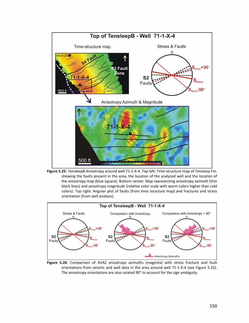
150
Figure 5.25: TensleepB Anisotropy around well 71‐1‐X‐4. Top left: Time‐structure map of Tensleep Fm. showing the faults present in the area, the location of the analyzed well and the location of the anisotropy map (blue square). Bottom center: Map representing anisotropy azimuth (thin black lines) and anisotropy magnitude (relative color scale with warm colors higher than cold colors). Top right: Angular plot of faults (from time structure map) and fractures and stress orientation (from well analysis).
Figure 5.26: Comparison of AVAZ anisotropy azimuths (magenta) with stress fracture and fault orientations from seismic and well data in the area around well 71‐1‐X‐4 (see Figure 5.25). The anisotropy orientations are also rotated 90° to account for the sign ambiguity.
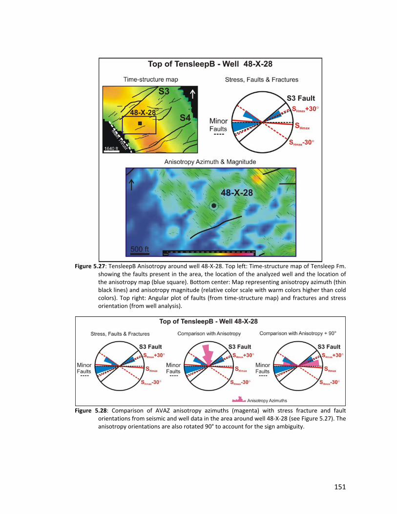
151
Figure 5.27: TensleepB Anisotropy around well 48‐X‐28. Top left: Time‐structure map of Tensleep Fm. showing the faults present in the area, the location of the analyzed well and the location of the anisotropy map (blue square). Bottom center: Map representing anisotropy azimuth (thin black lines) and anisotropy magnitude (relative color scale with warm colors higher than cold colors). Top right: Angular plot of faults (from time‐structure map) and fractures and stress orientation (from well analysis).
Figure 5.28: Comparison of AVAZ anisotropy azimuths (magenta) with stress fracture and fault orientations from seismic and well data in the area around well 48‐X‐28 (see Figure 5.27). The anisotropy orientations are also rotated 90° to account for the sign ambiguity.
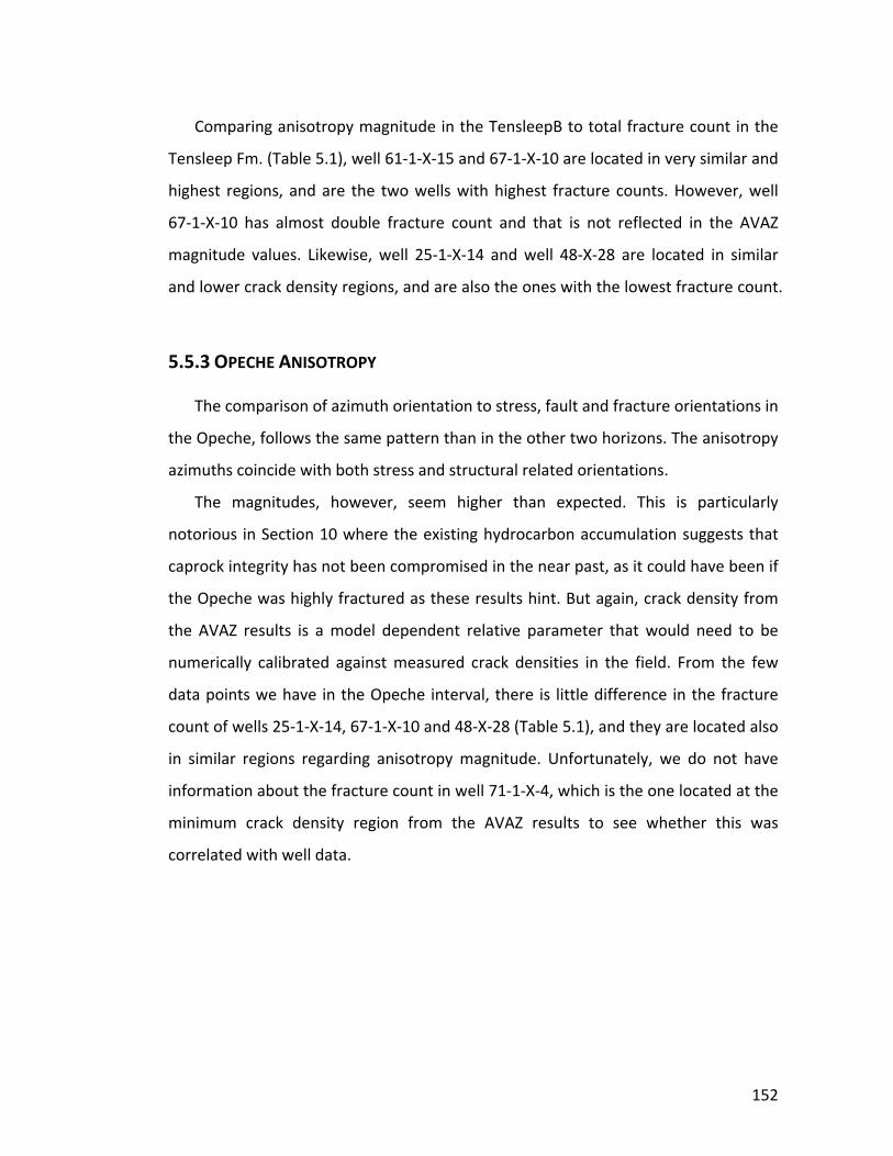
152
Comparing anisotropy magnitude in the TensleepB to total fracture count in the
Tensleep Fm. (Table 5.1), well 61‐1‐X‐15 and 67‐1‐X‐10 are located in very similar and
highest regions, and are the two wells with highest fracture counts. However, well
67‐1‐X‐10 has almost double fracture count and that is not reflected in the AVAZ
magnitude values. Likewise, well 25‐1‐X‐14 and well 48‐X‐28 are located in similar
and lower crack density regions, and are also the ones with the lowest fracture count.
5.5.3 OPECHE ANISOTROPY
The comparison of azimuth orientation to stress, fault and fracture orientations in
the Opeche, follows the same pattern than in the other two horizons. The anisotropy
azimuths coincide with both stress and structural related orientations.
The magnitudes, however, seem higher than expected. This is particularly
notorious in Section 10 where the existing hydrocarbon accumulation suggests that
caprock integrity has not been compromised in the near past, as it could have been if
the Opeche was highly fractured as these results hint. But again, crack density from
the AVAZ results is a model dependent relative parameter that would need to be
numerically calibrated against measured crack densities in the field. From the few
data points we have in the Opeche interval, there is little difference in the fracture
count of wells 25‐1‐X‐14, 67‐1‐X‐10 and 48‐X‐28 (Table 5.1), and they are located also
in similar regions regarding anisotropy magnitude. Unfortunately, we do not have
information about the fracture count in well 71‐1‐X‐4, which is the one located at the
minimum crack density region from the AVAZ results to see whether this was
correlated with well data.
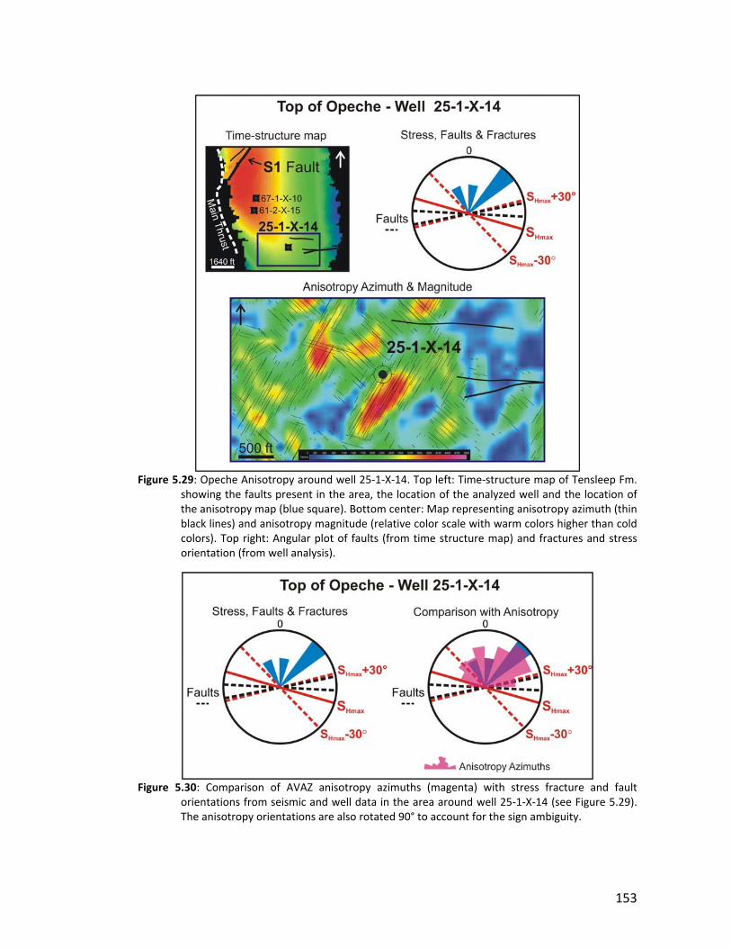
153
Figure 5.29: Opeche Anisotropy around well 25‐1‐X‐14. Top left: Time‐structure map of Tensleep Fm. showing the faults present in the area, the location of the analyzed well and the location of the anisotropy map (blue square). Bottom center: Map representing anisotropy azimuth (thin black lines) and anisotropy magnitude (relative color scale with warm colors higher than cold colors). Top right: Angular plot of faults (from time structure map) and fractures and stress orientation (from well analysis).
Figure 5.30: Comparison of AVAZ anisotropy azimuths (magenta) with stress fracture and fault orientations from seismic and well data in the area around well 25‐1‐X‐14 (see Figure 5.29). The anisotropy orientations are also rotated 90° to account for the sign ambiguity.
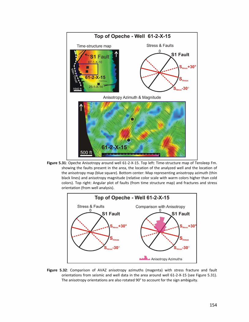
154
Figure 5.31: Opeche Anisotropy around well 61‐2‐X‐15. Top left: Time‐structure map of Tensleep Fm. showing the faults present in the area, the location of the analyzed well and the location of the anisotropy map (blue square). Bottom center: Map representing anisotropy azimuth (thin black lines) and anisotropy magnitude (relative color scale with warm colors higher than cold colors). Top right: Angular plot of faults (from time structure map) and fractures and stress orientation (from well analysis).
Figure 5.32: Comparison of AVAZ anisotropy azimuths (magenta) with stress fracture and fault
orientations from seismic and well data in the area around well 61‐2‐X‐15 (see Figure 5.31). The anisotropy orientations are also rotated 90° to account for the sign ambiguity.
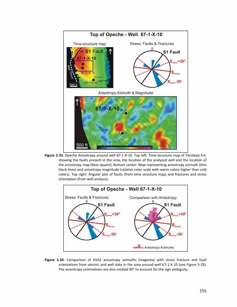
155
Figure 5.33: Opeche Anisotropy around well 67‐1‐X‐10. Top left: Time‐structure map of Tensleep Fm. showing the faults present in the area, the location of the analyzed well and the location of the anisotropy map (blue square). Bottom center: Map representing anisotropy azimuth (thin black lines) and anisotropy magnitude (relative color scale with warm colors higher than cold colors). Top right: Angular plot of faults (from time structure map) and fractures and stress orientation (from well analysis).
Figure 5.34: Comparison of AVAZ anisotropy azimuths (magenta) with stress fracture and fault
orientations from seismic and well data in the area around well 67‐1‐X‐10 (see Figure 5.33). The anisotropy orientations are also rotated 90° to account for the sign ambiguity.
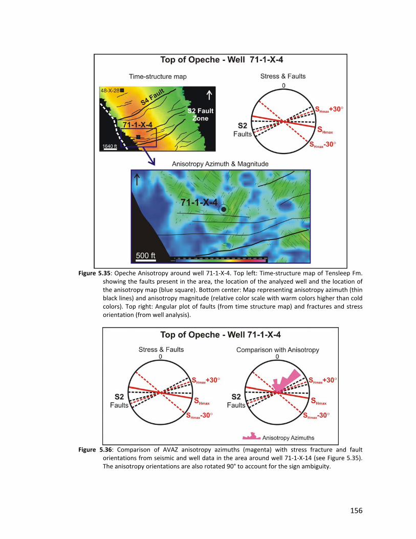
156
Figure 5.35: Opeche Anisotropy around well 71‐1‐X‐4. Top left: Time‐structure map of Tensleep Fm. showing the faults present in the area, the location of the analyzed well and the location of the anisotropy map (blue square). Bottom center: Map representing anisotropy azimuth (thin black lines) and anisotropy magnitude (relative color scale with warm colors higher than cold colors). Top right: Angular plot of faults (from time structure map) and fractures and stress orientation (from well analysis).
Figure 5.36: Comparison of AVAZ anisotropy azimuths (magenta) with stress fracture and fault orientations from seismic and well data in the area around well 71‐1‐X‐14 (see Figure 5.35). The anisotropy orientations are also rotated 90° to account for the sign ambiguity.
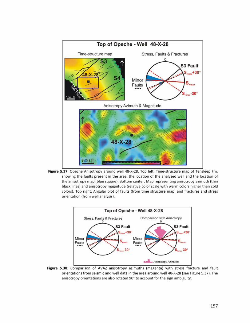
157
Figure 5.37: Opeche Anisotropy around well 48‐X‐28. Top left: Time‐structure map of Tensleep Fm. showing the faults present in the area, the location of the analyzed well and the location of the anisotropy map (blue square). Bottom center: Map representing anisotropy azimuth (thin black lines) and anisotropy magnitude (relative color scale with warm colors higher than cold colors). Top right: Angular plot of faults (from time structure map) and fractures and stress orientation (from well analysis).
Figure 5.38: Comparison of AVAZ anisotropy azimuths (magenta) with stress fracture and fault orientations from seismic and well data in the area around well 48‐X‐28 (see Figure 5.37). The anisotropy orientations are also rotated 90° to account for the sign ambiguity.
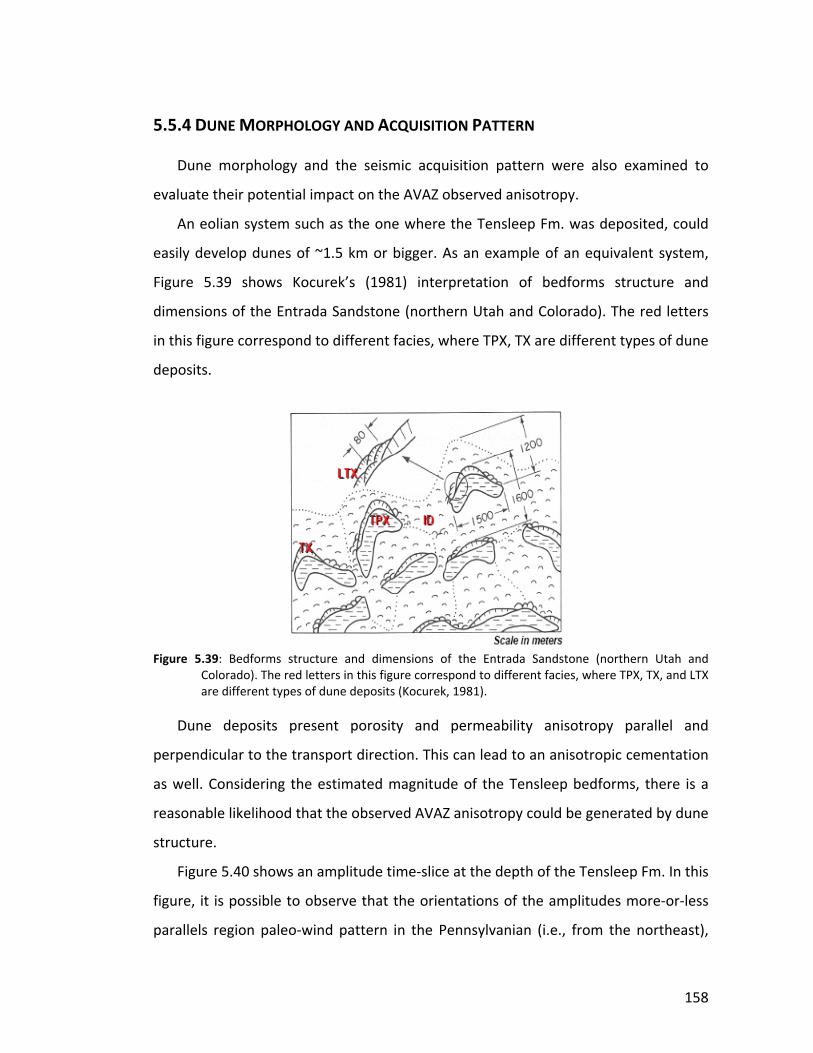
158
5.5.4 DUNE MORPHOLOGY AND ACQUISITION PATTERN
Dune morphology and the seismic acquisition pattern were also examined to
evaluate their potential impact on the AVAZ observed anisotropy.
An eolian system such as the one where the Tensleep Fm. was deposited, could
easily develop dunes of ~1.5 km or bigger. As an example of an equivalent system,
Figure 5.39 shows Kocurek’s (1981) interpretation of bedforms structure and
dimensions of the Entrada Sandstone (northern Utah and Colorado). The red letters
in this figure correspond to different facies, where TPX, TX are different types of dune
deposits.
Figure 5.39: Bedforms structure and dimensions of the Entrada Sandstone (northern Utah and Colorado). The red letters in this figure correspond to different facies, where TPX, TX, and LTX are different types of dune deposits (Kocurek, 1981).
Dune deposits present porosity and permeability anisotropy parallel and
perpendicular to the transport direction. This can lead to an anisotropic cementation
as well. Considering the estimated magnitude of the Tensleep bedforms, there is a
reasonable likelihood that the observed AVAZ anisotropy could be generated by dune
structure.
Figure 5.40 shows an amplitude time‐slice at the depth of the Tensleep Fm. In this
figure, it is possible to observe that the orientations of the amplitudes more‐or‐less
parallels region paleo‐wind pattern in the Pennsylvanian (i.e., from the northeast),
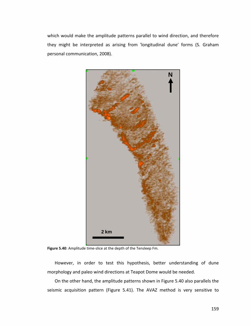
159
which would make the amplitude patterns parallel to wind direction, and therefore
they might be interpreted as arising from 'longitudinal dune' forms (S. Graham
personal communication, 2008).
Figure 5.40: Amplitude time‐slice at the depth of the Tensleep Fm.
However, in order to test this hypothesis, better understanding of dune
morphology and paleo wind directions at Teapot Dome would be needed.
On the other hand, the amplitude patterns shown in Figure 5.40 also parallels the
seismic acquisition pattern (Figure 5.41). The AVAZ method is very sensitive to
2 km
N
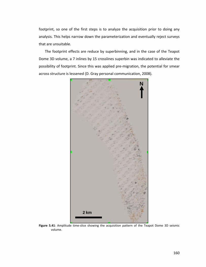
160
footprint, so one of the first steps is to analyze the acquisition prior to doing any
analysis. This helps narrow down the parameterization and eventually reject surveys
that are unsuitable.
The footprint effects are reduce by superbinning, and in the case of the Teapot
Dome 3D volume, a 7 inlines by 15 crosslines superbin was indicated to alleviate the
possibility of footprint. Since this was applied pre‐migration, the potential for smear
across structure is lessened (D. Gray personal communication, 2008).
Figure 5.41: Amplitude time‐slice showing the acquisition pattern of the Teapot Dome 3D seismic volume.
2 km
N
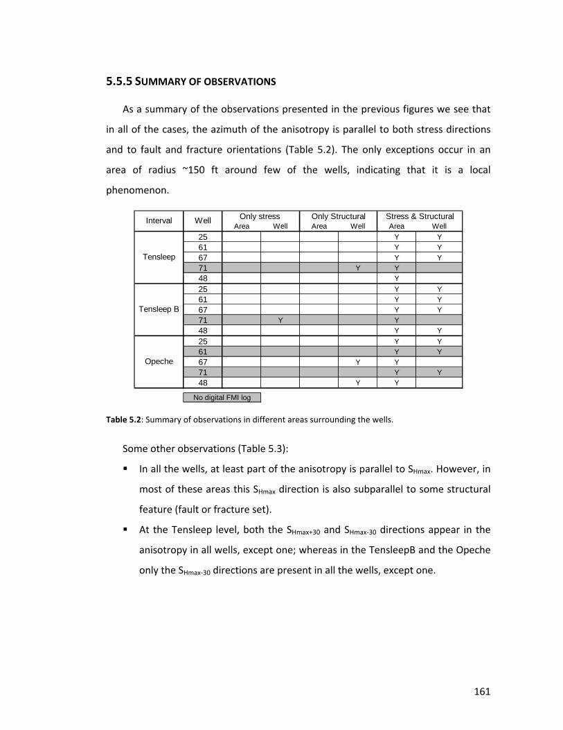
161
5.5.5 SUMMARY OF OBSERVATIONS
As a summary of the observations presented in the previous figures we see that
in all of the cases, the azimuth of the anisotropy is parallel to both stress directions
and to fault and fracture orientations (Table 5.2). The only exceptions occur in an
area of radius ~150 ft around few of the wells, indicating that it is a local
phenomenon.
Table 5.2: Summary of observations in different areas surrounding the wells.
Some other observations (Table 5.3):
In all the wells, at least part of the anisotropy is parallel to SHmax. However, in
most of these areas this SHmax direction is also subparallel to some structural
feature (fault or fracture set).
At the Tensleep level, both the SHmax+30 and SHmax‐30 directions appear in the
anisotropy in all wells, except one; whereas in the TensleepB and the Opeche
only the SHmax‐30 directions are present in all the wells, except one.
Area Well Area Well Area Well25 Y Y61 Y Y67 Y Y71 Y Y48 Y25 Y Y61 Y Y67 Y Y71 Y Y48 Y Y25 Y Y61 Y Y67 Y Y71 Y Y48 Y Y
Only stress Only Structural Stress & Structural
Tensleep
Interval Well
Tensleep B
Opeche
No digital FMI log
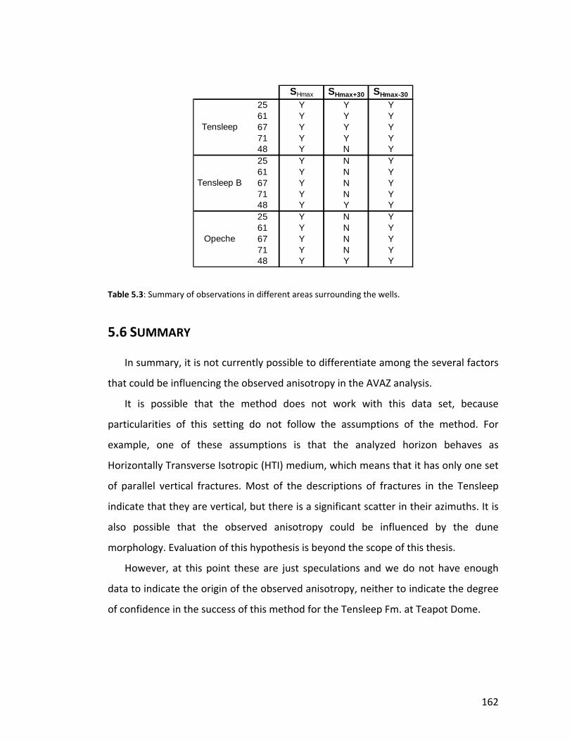
162
Table 5.3: Summary of observations in different areas surrounding the wells.
5.6 SUMMARY
In summary, it is not currently possible to differentiate among the several factors
that could be influencing the observed anisotropy in the AVAZ analysis.
It is possible that the method does not work with this data set, because
particularities of this setting do not follow the assumptions of the method. For
example, one of these assumptions is that the analyzed horizon behaves as
Horizontally Transverse Isotropic (HTI) medium, which means that it has only one set
of parallel vertical fractures. Most of the descriptions of fractures in the Tensleep
indicate that they are vertical, but there is a significant scatter in their azimuths. It is
also possible that the observed anisotropy could be influenced by the dune
morphology. Evaluation of this hypothesis is beyond the scope of this thesis.
However, at this point these are just speculations and we do not have enough
data to indicate the origin of the observed anisotropy, neither to indicate the degree
of confidence in the success of this method for the Tensleep Fm. at Teapot Dome.
SHmax SHmax+30 SHmax-3025 Y Y Y61 Y Y Y67 Y Y Y71 Y Y Y48 Y N Y25 Y N Y61 Y N Y67 Y N Y71 Y N Y48 Y Y Y25 Y N Y61 Y N Y67 Y N Y71 Y N Y48 Y Y Y
Opeche
Tensleep
Tensleep B
163
CHAPTER 6
USING MICROSEISMIC
STIMULATION TO ENHANCE
PERMEABILITY IN TIGHT
FORMATIONS
6.1 ABSTRACT
Deep saline formations have great potential for geologic sequestration of CO2. As
such formations are widespread in many parts of the U.S., they are in theory, easily
accessed from point sources of CO2, such as power plants, factories, refineries,
cement plants, etc. As typical of deep mature basins, many deep saline formations of
the mid‐continental U.S. appear to have very low porosity and permeability

164
compared to those encountered in large oil reservoirs, resulting in limited injectivity
and storage capacities.
A demonstration CO2 sequestration project was performed in the Michigan Basin,
the Otsego County Test Site, where potential targets for sequestration include
several Paleozoic reservoirs. In particular we analyze the Silurian Bass Island dolomite
(BILD) at approximately 1050 m depth. The source for this project is the associated
CO2 removed from the Antrim Shale gas at 6 centralized gas‐processing plants in the
Otsego County and other adjacent counties, which averages ~1.2 million metric tons
per year. A preliminary simple fluid flow simulation indicates that under the present
condition ~50% of this CO2 could be stored in the BILD.
During an injection‐induced microseismicity stimulation experiment, a total of
more than 10,000 metric tons of supercritical CO2 were injected into the BILD
formation during a period of 40 days. The objectives of the injection experiment
were to evaluate microseismic monitoring technologies and establishing the storage
capacity and suitability of the BILD, and potentially enhance the permeability and
injectivity of the target reservoir.
Microseismic stimulation is initiated by increasing the fluid pressure in the target
formation, thus reducing the effective normal stress on optimally‐oriented faults and
fractures triggering slip, and creating high‐permeability pathways within the reservoir.
This technique is a frequent and safe practice for imaging hydraulic fracturing
operations in the oil and gas industry, and enhancing permeability in geothermal
resources.
We have developed a preliminary geomechanical characterization as a base for
the proposed experiment. To develop the geomechanical model, we analyzed
formation micro‐image (FMI), density and sonic logs from two wells, as well as leak‐
off tests and pore pressure measurements from wells in the vicinity. This analysis also
provided us with the theoretical pressure needed to hydrofracture the target
formation and the expected fracture direction propagation.

165
Seismic monitoring of the injection was achieved by two downhole seismometer
arrays that consisted of eight, three‐component sensors each. The arrays were
deployed in two nearby monitoring wells directly above the target horizon at 150 m
and 550 m lateral distance to the injection point, respectively. The sensor spacing
was 15 m. Calibration shots in the injection well were used to determine the
orientation of the sensors at each depth in the two monitoring wells.
The analysis of the obtained microseismic data and the understanding of the
spatial‐temporal behavior of the induced microearthquakes are related to the
hydraulic parameters such as injection rate and well‐head pressure, which provide
valuable information on the resultant fluid‐flow network of the reservoir.
6.2 INTRODUCTION
One of the biggest challenges for CO2 sequestration in deep saline formations is
the very low porosity and permeabilities often shown, that translates into limited
injectivity and storage capacities.
Injection‐induced microseismicity has been frequently used in the oil industry to
enhance permeability. Increasing fluid pressure following hydraulic fracturing,
reduces the effective normal stress on optimally‐oriented faults and fractures,
therefore inducing slip and creating high‐permeability paths within the reservoir. The
induced failure is mainly triggered by a diffusive process of pore pressure
perturbation and often occurs as a sequence of many small events.
The volume of rock stimulated by hydraulic fracturing can be imaged by locating
these microearthquakes induced by the injection (Albright and Pearson, 1982) that
can be relocalized to show the geometry of slipping fractures. In addition to the
permeability enhancement and characterization of hydraulic fracture network,
microseismicity can potentially be used for the estimation of hydraulic properties of
rocks over large scales such as hydraulic diffusivity and permeability (Shapiro et al.,
2002).
166
Some examples of fluid induced microseismicity can be found in sedimentary
environments such as the Frio sandstone or the Cotton Valley tight gas sands. In
carbonate settings some examples include the Austin chalk and low porosity
Ordovician carbonate rocks in Clinton County, Kentucky. In crystalline rocks,
examples can be found in hot‐dry‐rock geothermal sites such as Fenton Hill, New
Mexico or Soultz, France (Phillips et al., 2002). Another remarkable example is the
Yufutsu oil and gas field, Japan, where injectivity was increased eight times after the
stimulation (Tezuka, 2006).
Therefore, it was proposed the use of microseismic stimulation to enhance the
permeability and injectivity in a tight formation; as well as the use of seismic
monitoring to gather information about the permeability and the fracture network of
the reservoir.
Passive seismic monitoring (PSM) started in the 30s and its growth was the result
of the interest in quantifying earthquake phenomena. The most notorious examples
in the use of this technique count Richter’s earthquake magnitude scale for regional
events in CA (1935) and the discovery of earthquake frequency‐magnitude relation
(Gutenberg and Richter, 1941). In the 60s, technical developments in seismic
networks and modern data processing allowed the application of PSM to detect and
analyze earthquakes over a broad range of magnitudes.
PSM is a tool used in a variety of applications such as mapping active faults at
different scales for hazard estimation, investigation of large earthquake phenomena
along plate‐bounding faults, and characterization of hydrocarbon and geothermal
reservoirs (Bohnhoff et al, in press). Recently, this technique has started to be
developed and tested to monitor underground storage of CO2 as in the project
described in this chapter.
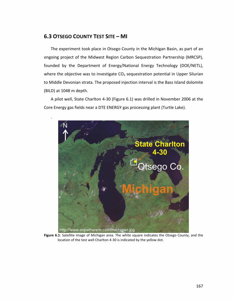
167
6.3 OTSEGO COUNTY TEST SITE – MI
The experiment took place in Otsego County in the Michigan Basin, as part of an
ongoing project of the Midwest Region Carbon Sequestration Partnership (MRCSP),
founded by the Department of Energy/National Energy Technology (DOE/NETL),
where the objective was to investigate CO2 sequestration potential in Upper Silurian
to Middle Devonian strata. The proposed injection interval is the Bass Island dolomite
(BILD) at 1048 m depth.
A pilot well, State Charlton 4‐30 (Figure 6.1) was drilled in November 2006 at the
Core Energy gas fields near a DTE ENERGY gas processing plant (Turtle Lake).
.
Figure 6.1: Satellite image of Michigan area. The white square indicates the Otsego County, and the location of the test well Charlton 4‐30 is indicated by the yellow dot.
168
The source for this project is the associated CO2 removed from the Antrim Shale
gas at 6 centralized gas‐processing plants in the Otsego Country and other adjacent
counties, which averages ~1.2 million metric tons per year. The CO2 is delivered to
the test site through an existing CO2 pipeline that Core Energy utilizes for several
CO2‐EOR projects that has been going at least since 2004 in the Otsego County. This
EOR projects targets the Paleozoic reefs at ~5000 ft depth, they are relatively small
floods involving 2 or 3 wells (Oil and Gas Journal Report, 2004). One of these floods
occurs just in these pilot areas ~1500 ft deeper and ~2000 ft north of one of the
monitoring wells.
6.3.1 TEST SITE GEOLOGY
Figure 6.2 shows the schematic stratigraphic column at well State Charlton 4‐30
from borehole logs, sidewall and conventional cores. The storage interval comprises
the BILD (injection target) and the Bois Blanc Formation, whereas the seal is the
Amherstburg Formation.
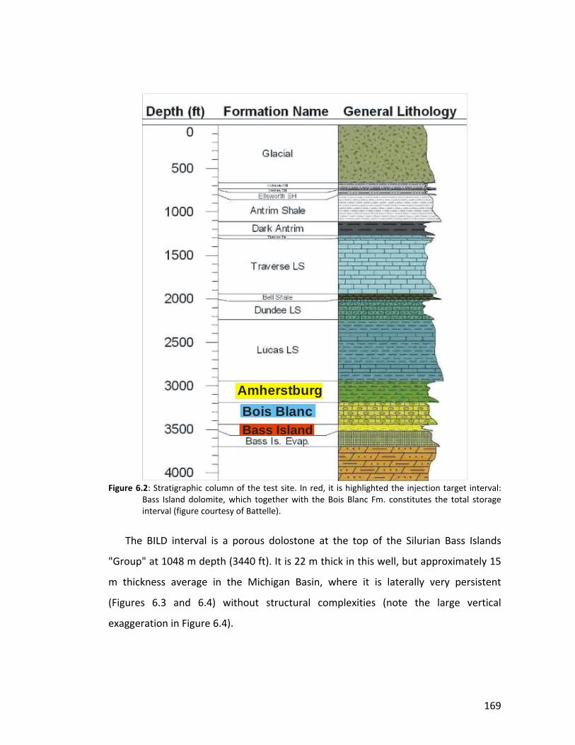
169
Figure 6.2: Stratigraphic column of the test site. In red, it is highlighted the injection target interval: Bass Island dolomite, which together with the Bois Blanc Fm. constitutes the total storage interval (figure courtesy of Battelle).
The BILD interval is a porous dolostone at the top of the Silurian Bass Islands
"Group" at 1048 m depth (3440 ft). It is 22 m thick in this well, but approximately 15
m thickness average in the Michigan Basin, where it is laterally very persistent
(Figures 6.3 and 6.4) without structural complexities (note the large vertical
exaggeration in Figure 6.4).
Amherstburg
Bass IslandBois Blanc

170
Figure 6.3: Structural map of Bass Island dolomite in Michigan, showing the location of Otsego Co. and
Well Charlton 4‐30. Modified from Barnes et al. (in press).
Porosity in the BILD ranges from less than 5% to more than 25%, and the average
porosity is 15%. The average permeability is less than 13 mD. Barnes et al. (in press)
performed a preliminary interpretation based on cores from the well State Charlton
4‐30, in which they suggested that this unit was deposited in a restricted marine,
possibly tidal flat to sabhka environment, with periodic and possibly protracted
subaerial exposure surfaces, that resulted in repeated karsted intervals. They
indicated that mineralized natural fractures are common.
Well Charlton 4-30
Otsego Co.
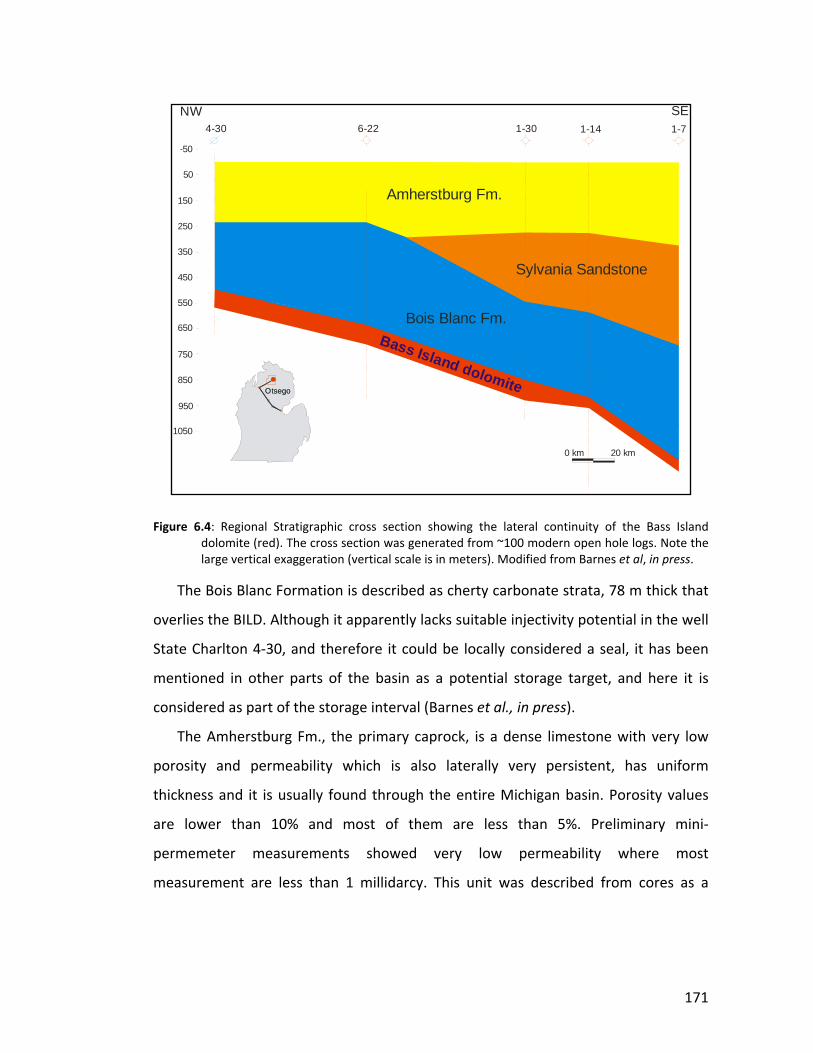
171
Figure 6.4: Regional Stratigraphic cross section showing the lateral continuity of the Bass Island
dolomite (red). The cross section was generated from ~100 modern open hole logs. Note the large vertical exaggeration (vertical scale is in meters). Modified from Barnes et al, in press.
The Bois Blanc Formation is described as cherty carbonate strata, 78 m thick that
overlies the BILD. Although it apparently lacks suitable injectivity potential in the well
State Charlton 4‐30, and therefore it could be locally considered a seal, it has been
mentioned in other parts of the basin as a potential storage target, and here it is
considered as part of the storage interval (Barnes et al., in press).
The Amherstburg Fm., the primary caprock, is a dense limestone with very low
porosity and permeability which is also laterally very persistent, has uniform
thickness and it is usually found through the entire Michigan basin. Porosity values
are lower than 10% and most of them are less than 5%. Preliminary mini‐
permemeter measurements showed very low permeability where most
measurement are less than 1 millidarcy. This unit was described from cores as a
4-30 6-22 1-30 1-14
0 km 20 km
NW SE
-50
50
150
250
350
450
550
650
750
850
1-7
950
1050
OtsegoOtsego
Amherstburg Fm.
Sylvania Sandstone
Bois Blanc Fm.Bass Island dolomite
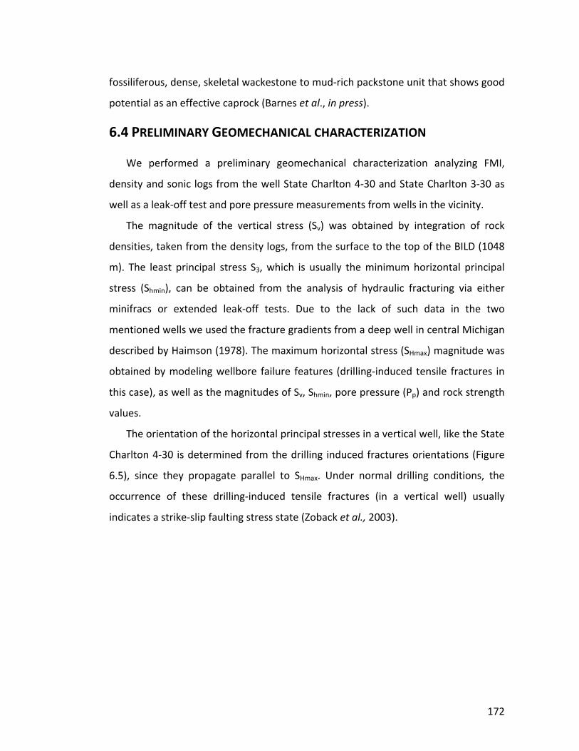
172
fossiliferous, dense, skeletal wackestone to mud‐rich packstone unit that shows good
potential as an effective caprock (Barnes et al., in press).
6.4 PRELIMINARY GEOMECHANICAL CHARACTERIZATION
We performed a preliminary geomechanical characterization analyzing FMI,
density and sonic logs from the well State Charlton 4‐30 and State Charlton 3‐30 as
well as a leak‐off test and pore pressure measurements from wells in the vicinity.
The magnitude of the vertical stress (Sv) was obtained by integration of rock
densities, taken from the density logs, from the surface to the top of the BILD (1048
m). The least principal stress S3, which is usually the minimum horizontal principal
stress (Shmin), can be obtained from the analysis of hydraulic fracturing via either
minifracs or extended leak‐off tests. Due to the lack of such data in the two
mentioned wells we used the fracture gradients from a deep well in central Michigan
described by Haimson (1978). The maximum horizontal stress (SHmax) magnitude was
obtained by modeling wellbore failure features (drilling‐induced tensile fractures in
this case), as well as the magnitudes of Sv, Shmin, pore pressure (Pp) and rock strength
values.
The orientation of the horizontal principal stresses in a vertical well, like the State
Charlton 4‐30 is determined from the drilling induced fractures orientations (Figure
6.5), since they propagate parallel to SHmax. Under normal drilling conditions, the
occurrence of these drilling‐induced tensile fractures (in a vertical well) usually
indicates a strike‐slip faulting stress state (Zoback et al., 2003).
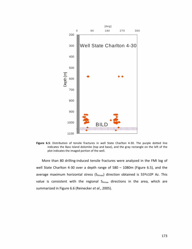
173
Figure 6.5: Distribution of tensile fractures in well State Charlton 4‐30. The purple dotted line
indicates the Bass Island dolomite (top and base), and the gray rectangle on the left of the plot indicates the imaged portion of the well.
More than 80 drilling‐induced tensile fractures were analyzed in the FMI log of
well State Charlton 4‐30 over a depth range of 580 – 1080m (Figure 6.5), and the
average maximum horizontal stress (SHmax) direction obtained is 55º±10º Az. This
value is consistent with the regional SHmax directions in the area, which are
summarized in Figure 6.6 (Reinecker et al., 2005).
200
300
400
500
600
700
800
900
1000
1100
0 90 180 270 360
BILD
Dept
h[m
]
Well State Charlton 4-30
[deg]
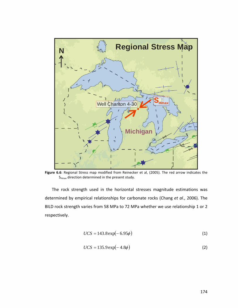
174
Figure 6.6: Regional Stress map modified from Reinecker et al, (2005). The red arrow indicates the SHmax direction determined in the present study.
The rock strength used in the horizontal stresses magnitude estimations was
determined by empirical relationships for carbonate rocks (Chang et al., 2006). The
BILD rock strength varies from 58 MPa to 72 MPa whether we use relationship 1 or 2
respectively.
( )φ95.6exp8.143 −=UCS (1)
( )φ8.4exp9.135 −=UCS (2)
Michigan
Well Charlton 4-30
N Regional Stress Map
SHmax

175
In summary, the analysis of the studied wells indicates a Strike Slip faulting stress
state (Figure 6.7), where SHmax ≈ 33 MPa, Sv = 26.6 MPa, Shmin ≈ 17.9 MPa (Haimson,
1978), and SHmax orientation = 55º ±10º Az. The pore pressure used in this analysis is
Pp = 10.8 MPa, slightly over hydrostatic.
Figure 6.7: Stress summary plot for well State Charlton 4‐30. At 1048 m depth (top of Bass Island
dolomite): Pp = 10.8 MPa (blue dot), SHmax ≈ 33 MPa (red diamond), Sv = 26.6 MPa (green square), Shmin ≈ 17.9 MPa (yellow triangle).
Under the present stress conditions, if the fluid pressure in the well exceeds the
magnitude of the least principal stress (Shmin), a vertical hydraulic fracture should
propagate in the plane normal to the Shmin direction, since they always propagate
perpendicular to the least principal stress in the earth (Hubbert and Willis, 1957).
Once the induced seismicity experiment takes place, we will have the empirical
value of Shmin, which is the upper‐bound pressure value to avoid hydrofracture the
formation during the sequestration phase.
0
200
400
600
800
1000
1200
1400
0 10 20 30 40 50
Shmin Sv SHmaxPp
Stress [MPa]
Dep
th [m
]
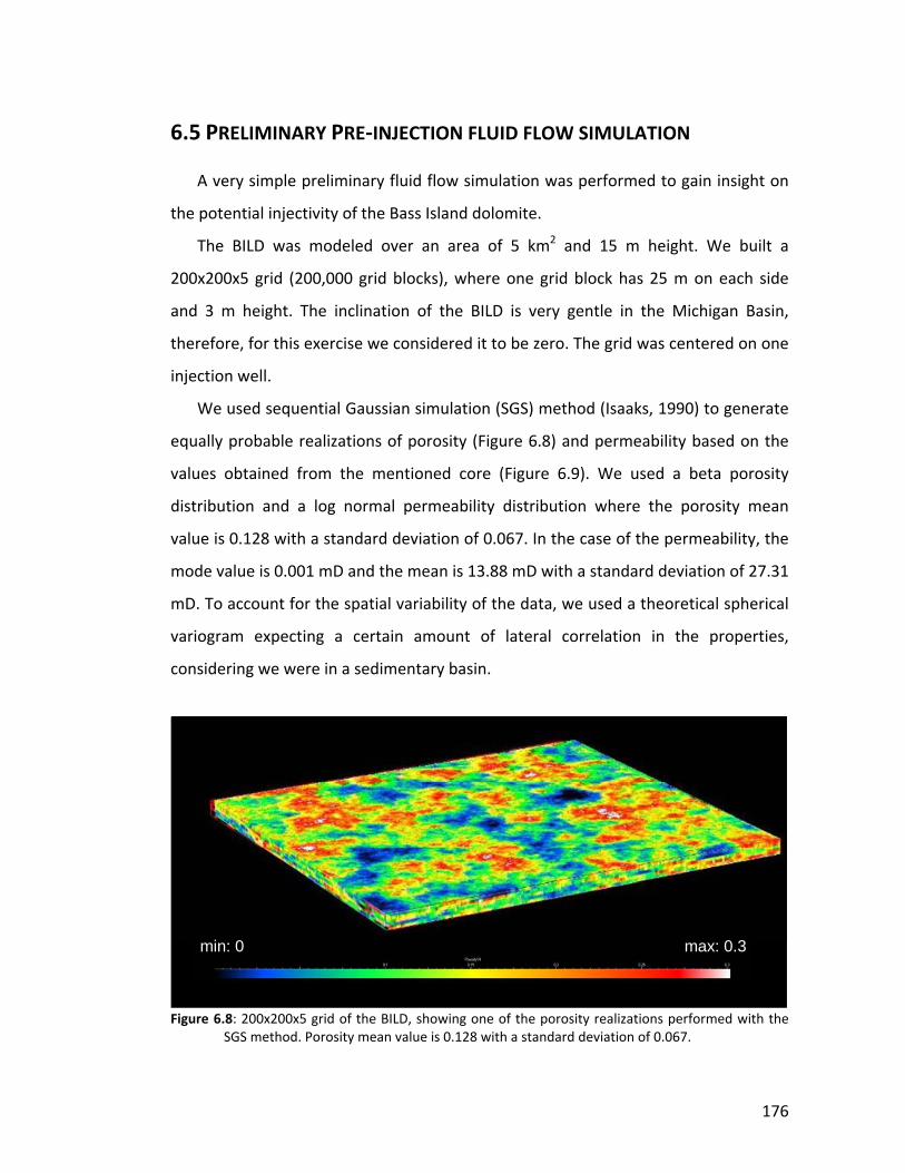
176
6.5 PRELIMINARY PRE‐INJECTION FLUID FLOW SIMULATION
A very simple preliminary fluid flow simulation was performed to gain insight on
the potential injectivity of the Bass Island dolomite.
The BILD was modeled over an area of 5 km2 and 15 m height. We built a
200x200x5 grid (200,000 grid blocks), where one grid block has 25 m on each side
and 3 m height. The inclination of the BILD is very gentle in the Michigan Basin,
therefore, for this exercise we considered it to be zero. The grid was centered on one
injection well.
We used sequential Gaussian simulation (SGS) method (Isaaks, 1990) to generate
equally probable realizations of porosity (Figure 6.8) and permeability based on the
values obtained from the mentioned core (Figure 6.9). We used a beta porosity
distribution and a log normal permeability distribution where the porosity mean
value is 0.128 with a standard deviation of 0.067. In the case of the permeability, the
mode value is 0.001 mD and the mean is 13.88 mD with a standard deviation of 27.31
mD. To account for the spatial variability of the data, we used a theoretical spherical
variogram expecting a certain amount of lateral correlation in the properties,
considering we were in a sedimentary basin.
Figure 6.8: 200x200x5 grid of the BILD, showing one of the porosity realizations performed with the SGS method. Porosity mean value is 0.128 with a standard deviation of 0.067.
min: 0 max: 0.3
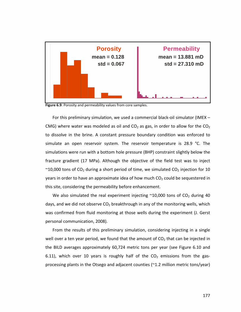
177
Figure 6.9: Porosity and permeability values from core samples.
For this preliminary simulation, we used a commercial black‐oil simulator (IMEX –
CMG) where water was modeled as oil and CO2 as gas, in order to allow for the CO2
to dissolve in the brine. A constant pressure boundary condition was enforced to
simulate an open reservoir system. The reservoir temperature is 28.9 °C. The
simulations were run with a bottom hole pressure (BHP) constraint slightly below the
fracture gradient (17 MPa). Although the objective of the field test was to inject
~10,000 tons of CO2 during a short period of time, we simulated CO2 injection for 10
years in order to have an approximate idea of how much CO2 could be sequestered in
this site, considering the permeability before enhancement.
We also simulated the real experiment injecting ~10,000 tons of CO2 during 40
days, and we did not observe CO2 breakthrough in any of the monitoring wells, which
was confirmed from fluid monitoring at those wells during the experiment (J. Gerst
personal communication, 2008).
From the results of this preliminary simulation, considering injecting in a single
well over a ten year period, we found that the amount of CO2 that can be injected in
the BILD averages approximately 60,724 metric tons per year (see Figure 6.10 and
6.11), which over 10 years is roughly half of the CO2 emissions from the gas‐
processing plants in the Otsego and adjacent counties (~1.2 million metric tons/year)
0 0.1 0.2 0.3 0.40
5
10
15
20
Porositymean = 0.128
std = 0.067
0 20 40 60 80 100 1200
10
20
30
40Permeability
mean = 13.881 mDstd = 27.310 mD
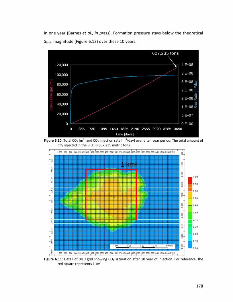
178
in one year (Barnes et al., in press). Formation pressure stays below the theoretical
Shmin magnitude (Figure 6.12) over these 10 years.
Figure 6.10: Total CO2 [m3] and CO2 injection rate [m
3/day] over a ten year period. The total amount of CO2 injected in the BILD is 607,235 metric tons.
Figure 6.11: Detail of BILD grid showing CO2 saturation after 10 year of injection. For reference, the red square represents 1 km2.
Time [days]
607,235 tonsC
umul
ativ
ega
s[m
3 ]
Gas
Rat
e[m
3 /da
y]
0.E+00
5.E+07
1.E+08
2.E+08
2.E+08
3.E+08
3.E+08
4.E+08
0 365 730 1095 1460 1825 2190 2555 2920 3285 36500
20,000
40,000
60,000
80,000
100,000
120,000
0 365 730 1095 1460 1825 2190 2555 2920 3285 3650
1 km2
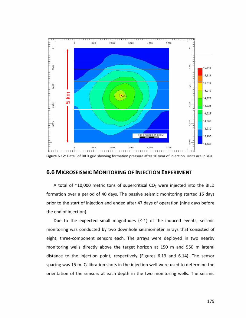
179
Figure 6.12: Detail of BILD grid showing formation pressure after 10 year of injection. Units are in kPa.
6.6 MICROSEISMIC MONITORING OF INJECTION EXPERIMENT
A total of ~10,000 metric tons of supercritical CO2 were injected into the BILD
formation over a period of 40 days. The passive seismic monitoring started 16 days
prior to the start of injection and ended after 47 days of operation (nine days before
the end of injection).
Due to the expected small magnitudes (≤‐1) of the induced events, seismic
monitoring was conducted by two downhole seismometer arrays that consisted of
eight, three‐component sensors each. The arrays were deployed in two nearby
monitoring wells directly above the target horizon at 150 m and 550 m lateral
distance to the injection point, respectively (Figures 6.13 and 6.14). The sensor
spacing was 15 m. Calibration shots in the injection well were used to determine the
orientation of the sensors at each depth in the two monitoring wells. The seismic
5 km
5 km
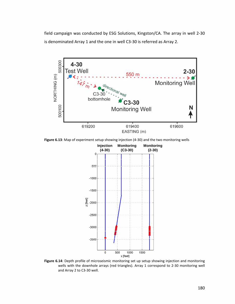
180
field campaign was conducted by ESG Solutions, Kingston/CA. The array in well 2‐30
is denominated Array 1 and the one in well C3‐30 is referred as Array 2.
Figure 6.13: Map of experiment setup showing injection (4‐30) and the two monitoring wells
Figure 6.14: Depth profile of microseismic monitoring set up setup showing injection and monitoring wells with the downhole arrays (red triangles). Array 1 correspond to 2‐30 monitoring well and Array 2 to C3‐30 well.
Injection(4-30)
Monitoring(C3-30)
Monitoring(2-30)
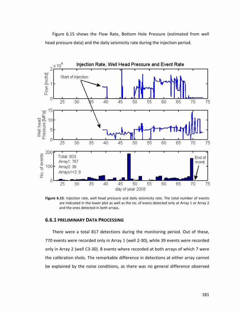
181
Figure 6.15 shows the Flow Rate, Bottom Hole Pressure (estimated from well
head pressure data) and the daily seismicity rate during the injection period.
Figure 6.15: Injection rate, well head pressure and daily seismicity rate. The total number of events are indicated in the lower plot as well as the no. of evens detected only at Array 1 or Array 2 and the ones detected in both arrays.
6.6.1 PRELIMINARY DATA PROCESSING
There were a total 817 detections during the monitoring period. Out of these,
770 events were recorded only in Array 1 (well 2‐30), while 39 events were recorded
only in Array 2 (well C3‐30). 8 events where recorded at both arrays of which 7 were
the calibration shots. The remarkable difference in detections at either array cannot
be explained by the noise conditions, as there was no general difference observed
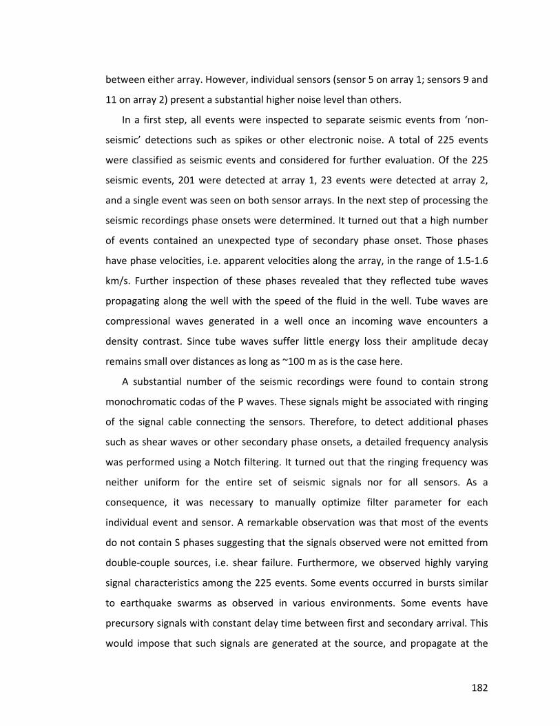
182
between either array. However, individual sensors (sensor 5 on array 1; sensors 9 and
11 on array 2) present a substantial higher noise level than others.
In a first step, all events were inspected to separate seismic events from ‘non‐
seismic’ detections such as spikes or other electronic noise. A total of 225 events
were classified as seismic events and considered for further evaluation. Of the 225
seismic events, 201 were detected at array 1, 23 events were detected at array 2,
and a single event was seen on both sensor arrays. In the next step of processing the
seismic recordings phase onsets were determined. It turned out that a high number
of events contained an unexpected type of secondary phase onset. Those phases
have phase velocities, i.e. apparent velocities along the array, in the range of 1.5‐1.6
km/s. Further inspection of these phases revealed that they reflected tube waves
propagating along the well with the speed of the fluid in the well. Tube waves are
compressional waves generated in a well once an incoming wave encounters a
density contrast. Since tube waves suffer little energy loss their amplitude decay
remains small over distances as long as ~100 m as is the case here.
A substantial number of the seismic recordings were found to contain strong
monochromatic codas of the P waves. These signals might be associated with ringing
of the signal cable connecting the sensors. Therefore, to detect additional phases
such as shear waves or other secondary phase onsets, a detailed frequency analysis
was performed using a Notch filtering. It turned out that the ringing frequency was
neither uniform for the entire set of seismic signals nor for all sensors. As a
consequence, it was necessary to manually optimize filter parameter for each
individual event and sensor. A remarkable observation was that most of the events
do not contain S phases suggesting that the signals observed were not emitted from
double‐couple sources, i.e. shear failure. Furthermore, we observed highly varying
signal characteristics among the 225 events. Some events occurred in bursts similar
to earthquake swarms as observed in various environments. Some events have
precursory signals with constant delay time between first and secondary arrival. This
would impose that such signals are generated at the source, and propagate at the
183
same velocity. Based on the signal frequency and event strength, we classified the
events into events with 1) only P waves, 2) P and S phase onsets, 3) a low‐frequency
onset (~100Hz), 4) a precursory phase, 5) swarm‐type behavior. Furthermore, we
observed an event‐triplet, i.e. three events with highly similar waveforms occurring
within a few seconds. This triplet is likely to reflect multiple activation of the same
source spot.
The phase velocity of the P waves across the arrays is uniformly in the range of
4.7‐5.3 km/s. This would imply that the source cannot be located far from the sensor
arrays. Furthermore, arrival times are earliest at one of the inner sensors in most
cases, what suggests that the events were generated at the depth of the sensor with
earliest arrival time. This observation was clearly unexpected as the sensor arrays
initially were deployed to monitor injection‐induced seismicity within the BILD
formation below the array. Applying a conventional hypocenter determination
procedure to the arrival time data, we confirmed that most of the events occurred in
direct vicinity of the respective sensor array. A possible interpretation of such a
hypocentral distribution would be that CO2 from the deeper injection (described in
Section 6.3) is migrating upwards along the monitoring wells. This is in good
agreement with the temporal evolution of the events that shows that almost all
detected seismic events occurred before the injection into the BILD formation
started. Instead, the maximum of the seismicity rate was observed when the deeper
injection stopped, which is a common observation derived from other injection
experiments.
6.7 SUMMARY
An injection‐induced microseismicity experiment took place in the Michigan Basin
in order to enhance permeability and injectivity of the potential storage reservoir:
the Bass Island dolomite (BILD) at ~1050 m depth. The experiment consisted in the
184
injection of ~10,000 tons of CO2 during a period of 40 days, while microseismic
monitoring was in place during 31 days during the injection.
A preliminary geomechanical characterization indicates a Strike Slip present day
stress state with a maximum horizontal stress (SHmax) direction of 55° Az. The
theoretical estimated value of the least principal stress (Shmin) is approximately 17.9
MPa. The injection pressure during the complete experiment was below this value.
Analysis of the microseismic monitoring data highlighted the risk of using
automated traditional data processing approaches where tube waves where
incorrectly interpreted as S waves. The presence of these tube waves, with strong
amplitudes, masked the week S wave signals. A detailed frequency filtering analysis
was performed in each event, to extract all the signals.
A total of 803 events were recorded in more than 3 sensors in each of the two
monitoring arrays. However, no definite seismic activity could be related to the
injection in the BILD. Perhaps, this was due to the small injection pressure or to
higher porosity and permeability than anticipated.
A remarkable observation was that most of the events do not contain S phases
suggesting that the signals observed were not emitted from double‐couple sources,
i.e. shear failure.
Applying a conventional hypocenter determination procedure to the arrival time
data, it was confirmed that most of the events occurred in direct vicinity of the
respective sensor array. A possible interpretation of such a hypocentral distribution
would be that CO2 from the deeper injection (described in Section 6.3) is migrating
upwards along the monitoring wells. This is in good agreement with the temporal
evolution of the events, that shows that almost all detected seismic events occurred
before the injection into the BILD formation started. Instead, the maximum of the
seismicity rate was observed when the deeper injection stopped, which was a
common observation derived from other injection experiments.
185
REFERENCES Albright, J.N. and Pearson, C.F., 1982, Acoustic emissions as a tool for hydraulic fracture
location: Experience at the Fenton Hill Hot Dry Site: J. Soc. Pet. Eng., 22, 523‐530l. Aziz, K. and Settari, A., 1979, Petroleum Reservoir Simulation, Applied Science Publishers,
New York. Bachu, S. and J.C. Shaw, 2004, CO2 Storage in Oil and Gas Reservoirs in Western Canada:
Effect of Aquifers, Potential for CO2‐Flood Enhanced Oil Recovery and Practical Capacity, In: E.S.Rubin, D.W.Keith and C.F.Gilboy (Eds.), Proceedings of 7th International Conference on Greenhouse Gas Control Technologies. Volume 1: Peer‐Reviewed Papers and Plenary Presentations, IEA Greenhouse Gas Programme, Cheltenham, UK.
Barnes, D.A., Wahr, A., Harrison, W.B. III, Grammer, G.M., and Gupta, N., in press Geological Carbon Sequestration Potential in Devonian Saline Aquifers of the Michigan Basin, AAPG/EMD/DEG Special Publication on Geological Sequestration of CO2.
Beaubien, S.E., S. Lombardi, G. Ciotoli, A. Annunziatellis, G. Hatziyannis, A. Metaxas and J. Pearce, 2004, Potential hazards of CO2 leakage in storage systems ‐ learning from natural systems, In: E.S.Rubin, D.W.Keith and C.F.Gilboy (Eds.), Proceedings of 7th International Conference on Greenhouse Gas Control Technologies. Volume 1: Peer‐Reviewed Papers and Plenary Presentations, IEA Greenhouse Gas Programme, Cheltenham, UK.
Beecy, D.J. and V.A. Kuuskraa, 2001, Status of U.S. Geologic Carbon Sequestration Research and Technology, Environmental Geosciences, V. 8, No. 3, pp. 152‐159.
Beinkafner, K., 1986, Use of dipmiter logs to refine structural mapping of Teapot Dome, Wyoming. AAPG Bulletin 70 (8): 1031
186
Bielinsky, A., A. Ebigbo, A. Kopp, H. Class, R. Helmig, 2005, Numerical Simulation of CO2 Storage in Geological Formations using MUFTE‐UG, Workshop on Leakage Modeling, Princeton, http://www.princeton.edu/~cmi/events/Geological%20Storage%20Workshop.htm
Bird, P., 1998, Kinematic history of the Laramide orogeny in latitudes 35‐49N, western United States: Tectonics, v. 17, p. 780‐801.
Blasing, T.J., 2008, Recent greenhouse gas concentrations, Carbon Dioxide Information Analysis Center, http://cdiac.ornl.gov/pns/current_ghg.html, updated September 2008.
Bleizeffer, D., 2008, Company must curb CO2 venting, Casper Star Tribune Online, http://www.trib.com/articles/2008/06/11/news/wyoming/201ccad6c089b30387257464007f288a.txt
Boness, N., 2005, Physical Properties and Multi‐Scale Seismic Anisotropy in the Crust Surrounding the San Andreas Fault Near Parkfield, CA, Doctoral Thesis, Stanford University.
Boness, N. L., and Zoback, M. D., 2004, Stress‐induced seismic velocity anisotropy and physical properties in the SAFOD Pilot Hole in Parkfield, CA: Geophys. Res. Lett., 31, L15S17.
Bohnhoff, M., Dresen, G., Ellsworth, W.L., Ito, H., in press, Passive Seismic Monitoring of natural and induced earthquakes: Case studies and socio‐economic relevance. In: S.Cloetingh and J.Negendank (eds.), ILP volume 'New Frontiers in Integrated Solid Earth Sciences'.
Brook, E.J., 2005, Tiny bubbles tell all, Science Vol 310, pp. 1285 – 1287, 25 November. Brown, K.M., Bekins, B., Clennell, B., Dewhurst, D. and Westbrook, G.K., 1994,
Heterogeneous hydrofracture development and accretionary fault dynamics. Geology (22): 259‐262.
Bruant, R.G., M.A. Celia, A.J. Guswa and C.A. Peters, 2002, Safe storage of CO2 in deep saline aquifers, V. 36, n. 11, pp. 240A‐245A.
Business and Economic Development Interim Committee, October 6th. http://www.wyopipeline.com/mission/Carbon%20Dioxide%20White%20Paper.pdf
Center for Global Development, 2007, Carbon Dioxide Emissions From Power Plants Rated Worldwide. ScienceDaily. Retrieved September 27, 2008, from http://www.sciencedaily.com /releases/2007/11/071114163448.htm
Chang, C., Zoback, M.D. and Khaksar, A., 2006, Empirical relations between rock strength and physical properties in sedimentary rocks: Journal of Petroleum Science and Engineering 51, 223‐237.
Chiaramonte, L., Zoback, M., Friedmann, J. and Stamp, V., 2008, Seal Integrity and Feasibility of CO2 Sequestration in the Teapot Dome EOR Pilot: Geomechanical Site Characterization. Environmental Geology, Volume 54, Number 8, 1667‐1675(9).
Chopra, A.K., Stein, M.H., and Dismuke, C.T., 1990, Prediction of Performance of Miscible‐Gas Pilots. JPT, December, pp. 1564‐1572.
Cooper, S.P. and Goodwin, L.B., 1998, Fracture characterization and variability within a basement‐cored Laramide age anticline, Teapot Dome, Wyoming. AAPG Annual Convention Abstract
187
Cooper, S.P., Lorenz, J.C. and Goodwin, L.B, 2001, ‘Lithologic and Structural Controls on Natural Fracture Characteristics Teapot Dome, Wyoming,” Sandia Report, contract No. DE‐AC04‐94AL85000, U.S. DOE , Albuquerque, NM.
Cooper, S.P., Hart, B., Goodwin, L.B., Lorenz, J.C., and Milliken, M., 2003, Outcrop and Seismic Analysis of Natural Fractures, Faults and Structure at Teapot Dome, Wyoming: Wyoming Geological Association 2003 Field Guidebook.
Crampin, S., 1984, Anisotropy in exploration seismic: First Break, March, 19‐21. Crampin, S., 1985, Evidence for aligned cracks in the Earth’s crust: First Break, Vo. 3, No,
3, 12‐15. Crampin, S., 1987, Geological and industrial implications of extensive‐dilatancy
anisotropy: Nature, 328, 491‐496. Crampin, S., Chesnokov, E. M., and Hipkin, R. G., 1984, Seismic anisotropy ‐ the state of
the art II: Geophys. J. R. astr. Soc. , 76, 1‐16. Crampin, S., and Lovell, J. H., 1991, A decade of shear‐wave splitting in the Earth's crust:
what does it mean? what use can we make of it? and what should we do next?: Geophys. J. Int., 107, 387‐407.
Dickinson, W.R. and Snyder, W.S., 1978, Plate tectonics of the Laramide orogeny: Geological Society of America Memoir 151, p. 355‐366.
Dake, L.P., 1978, Fundamentals of Reservoir Engineering, Chapter 9, Elsevier Scientific Publishing Co.
Dria, D.E., Pope, G.A,. and Sepehrnoori, K., 1993. Three‐Phase Gas/Oil/Brine Relative Permeabilities Measured Under CO2 Flooding Conditions, SPERE, May, pp. 143.
Doughty, C. and K. Preuss, 2004, Modeling Supercritical carbon dioxide injection in heterogeneous porous media. Vadose Zone Journal, V.3, pp. 837‐847.
Earth Decision ‐ Gocad 2.1.6 Software Energy & Minerals Field Institute (Emfi), 2004, ChevronTexaco’s Rangely Oil Field
Operations, http://inside.mines.edu/Outreach/cont_ed/emfi/emfi2005/ChevronTexaco.pdf
Emmet, W.R., Beaver, K.W. and McCaleb, J.A., 1972, Pennsylvanian Tensleep Reservoir, Little Buffalo Oil field, Big Horn Basin, Wyoming: The Mountain Geologist, V.9, No. 1, p. 21‐31.
Encyclopedia Britannica Online, accessed October 2008 http://www.britannica.com/EBchecked/topic/585252/Teapot‐Dome‐Scandal
Falkowski P, RJ Scholes, E. Boyle, J. Canadell, D. Canfield, J. Elser, N. Gruber, K. Hibbard, P. Högberg, S. Linder, F.T. Mackenzie, B. Moore III, T. Pederson, Y. Rosenthal, S. Seitzinger, V. Smetacek, W. Steffen, 2000, The Global Carbon Cycle: A Test of our Knowledge of Earth as a System, Science 290: 291‐296.
Finkbeiner, T., Zoback, M.D., Flemings, P. and Stump, B., 2001, Stress, pore pressure, and dynamically constrained hydrocarbon columns in the South Eugene Island 330 Field, northern Gulf of Mexico. American Association of Petroleum Geologists 85 (6): 1007‐1031
Flodin, E.A., 2003, Structural Evolution, Petrophysics, and Large‐Scale Permeability of Faults in Sandstone, Valley of Fire, Nevada [Ph.D. Thesis]: Stanford University, 180 pp.
188
Friedmann, S.J., Nummedal, D., Stamp, V.W., 2004, Science and technology goals of the Teapot Dome field experimental facility. NETL 3rd Annual Carbon Sequestration Conference Proceedings, Alexandria, VA, Exchange Monitor Publications
Friedmann, S.J. and Stamp, V.W., 2006, Teapot Dome: Characterization of a CO2‐enhanced oil recovery and storage site in Eastern Wyoming: Environmental Geosciences, v. 13, no. 3, pp. 181–199
Gaines, J., 2008, Monell Unit CO2 Flood, Patrick Draw Field, Sweetwater County, Wyoming. http://eori.uwyo.edu/downloads/CO2Conf_%20May2008/Jason%20Gaines_Anadarko_EORI_CO2%20Casper%20May%2029%202008.pdf
Gale, J., 2004, Geologic storage of CO2: What do we know, where are the gaps and what more needs to be done?, Energy v. 29, pp. 1329‐1338.
GEO‐SEQ Project Team, GEO‐SEQ Best Practice Manual, Geologic Carbon Dioxide Sequestration: Site Evaluation to Implementation, 2004, Earth Sciences Division, Ernest Orlando Lawrence Berkeley National Laboratory, Berkeley, CA, 40 pp.
Grasso, J.R., 1992, Mechanics of seismic instabilities induced by the recovery of hydrocarbon. Pure and Applied Geophysics 139 (3/4):507‐533
Gray, F.D., Head, K.J., Chamberlain, C.K., Olson, G., Sinclair, J. and Besler, C., 1999, Using 3D Seismic to Identify Spatially Variant Fracture Orientation in the Manderson Field, paper SPE 5636 presented at the 1999 SPE Rocky Mountain Regional Meeting, Gillette, WY, May 15‐18, 1999 Canadian SEG meeting abstracts, 59‐63, 1999 Rocky Mountain Association of Geologists and Denver Geophysical Society 3D Seismic Symposium Expanded Abstracts, CSEG Recorder, 24, 8, AAPG Explorer, September.
Gray, D., Boerner, S., Toodorovic‐Marinic, D. and Zheng, Y., 2003, Analyzing fractures from seismic for improved drilling success, World Oil, Vol. 224, No. 10, http://www.worldoil.com/magazine/MAGAZINE_DETAIL.asp?ART_ID=2133&MONTH_YEAR=Oct‐2003
Gray, D. and Todorovic‐Marinic, D. 2004, Fracture Detection using 3D Azimuthal AVO, CSEG RECORDER, http://www.cseg.ca/publications/recorder/2004/12dec/dec04‐fracture‐detection.pdf.
Gray, D., 2008, Fracture Detection Using 3D Seismic Azimuthal AVO, CSEG RECORDER, March 2008, pp. 34‐43.
Gringarten, 2005. Practice of 3D Modeling; Talk at Stanford University, PE 246 class (https://coursework‐ .stanford.edu/coursework/servlet/ShowFile?contentid=300119
Gutemberg, B. and Ritcher, C.F., 1941, Seismic of the earth, Geol Soc Am Spec Pap 34:1‐133
Haimson, B.C., 1978, Crustal Stress in the Michigan Basin: Journal of Geophysical Research, 83, 5857‐5863.
Hall, S.A, J.M. Kendall, O.I. Barkved, 2002, Fractured reservoir characterization using P‐wave AVOA analysis of 3D OBC data, The Leading Edge 21 (8): 777.
Hassler, B., 2006, Carbon Dioxide White Paper Prepared for the Wyoming Joint Minerals, Hennings, P., Zahm, C., Olson J. And Erslev, E. (2008), Geologic Occurrence and Hydraulic
Significance of Fractures in Reservoirs – Field Trip Guidebook, AAPG‐SPE‐SEG Hedberg Research Conference, Casper, WY.
189
Hubbert, M.K. and Willis, D.G., 1957, Mechanics of hydraulic fracturing: Pet Trans AIME, 210, 153‐63.
Hycal Energy Research Laboratories Ltd., 2004, DOE‐RMOTC, Teapot Dome Miscibility study, final report, December 13, 2004, 29 p.
ICPP Special Report, 2005, Carbon Dioxide Capture and Storage, ISBN 92‐9169‐119‐4, http://www.ipcc.ch/activity/ccsspm.pdf
IEA Greenhouse Gas R&D Programme, 2005, Greenhouse gases, information sheet, http://www.ieagreen.org.uk/1.pdf
IEA Greenhouse Gas R&D Programme, 2001, Putting Carbon back into the ground, ISBN 1 898373 28 0, http://www.ieagreen.org.uk/putcback.pdf
Isaaks, E. H., 1990, The application of Monte Carlo methods to the analysis of spatially correlated data: Ph.D. thesis, Stanford University, Stanford, California, 213 p.
Jahn, F., Cook, M. and Graham, M., 1998, Hydrocarbon exploration and production. Elsevier Amsterdam, 384 pp.
Jaeger, J.C. and N.G.W. Cook, 1969, Fundamentals of rock mechanics, Chapman and Hall, New York, 593 pp.
Jarrell, P.M., Fox, C.E., Stein, M.H. and Webb, S.L., 2002, Practical Aspects of CO2 Flooding. Monograph 22, Society of Petroleum Engineers, Richardson, TX, USA.
Jenner, E., 2001, Azimuthal anisotropy of compressional wave seismic data, Weyburn field, Saskatchewan, Canada, PhD Thesis, Colorado School of Mines.
Jenner, E., 2002, Azimuthal AVO: Methodology and data examples, The Leading Edge 21 (8): 782.
Jenssen, K. and F.M. Orr, 2002, Compositional streamline simulation, SPE Paper, 77379, SPE Annual Technical Conference and Exhibition, San Antonio, TX, Sept. 29‐Oct.2.
Jessen K., Kovscek A.R., Orr Jr F.M., 2005, Increasing CO2 storage in oil recovery. Energy Convers Manage 46(2): 293–311.
Journel, A.G., 1994, Geostatistics and reservoir geology, in Computer Applications3: Modeling and Geostatistics, Eds., J.M., Yarus and R.L., Chambers, AAPG, 19‐20.
Kocurek G., 1981. Erg reconstruction: the Entrada Sandstone (Jurassic) of northern Utah and Colorado. Palaeogeography, Palaeoclimatology, Palaeoecology 36, 125‐153.
Kovscek, A.R. and M.D. Cakici, 2005, Geologic storage of carbon dioxide and enhanced oil recovery. II. Cooptimization of storage and recovery. Energy Conversion and Management 46, 1941–1956
Kovascek, A.R. and Y. Wang, 2005, Geologic storage of carbon dioxide and enhanced oil recovery I: Uncertainty quantification employing a streamline‐based proxy for reservoir flow simulation, Energy Conversion and Management, in press, 2005.
Lorenz, J. C., and S. P. Cooper, 2004, Analysis of fracture characteristics and distribution of 48‐X‐28 well: Rocky Mountain Oilfield Testing Center Report, 31 p.
Lorenz, J.C., 2007, Summary of Published Information on Tensleep Fractures: http://eori.uwyo.edu/downloads/Tensleep_FractureStudy1.doc
Lucier, A., Zoback, M.D., Gupta, N. and Ramakrishnan, T.S., 2006, Geomechanical aspects of CO2 sequestration in a deep saline reservoir in the Ohio River Valley region: Environmental Geosciences, 13 (2), 85–103.
190
McCutcheon, T., 2003, Time Structure Maps – 3D Seismic Data Interpretation, Teapot Dome Oil Field, Naval Petroleum Reserve No. 3, Natrona County, Wyoming. Rocky Mountain Oilfield Testing Center Report Melzer, S.L., 2007. http://eori.uwyo.edu/downloads/Steve%20Melzer%20Oct%2025%20Presentation.pdf
Milliken, M.D., 2005, Surface Mapping Validates 3D Seismic Faulting Interpretations at Teapot Dome Field, Natrona Co., Wyoming. http://www.searchanddiscovery.com/documents/abstracts/2005rocky/RMmilli.htm
Milliken, M.D. and Koepsell, R., 2003, Imaging Technology offers enhanced interpretation of Teapot Dome reservoirs. Wyoming Geological Association Field Guidebook 2002: 41‐62
Miller, E. L., M. M. Miller, C. H. Stevens, J. E. Wright, and R. Madrid, 1992, Late Paleozoic paleogeographic and tectonic evolution of the western U.S. Cordillera, in B. C. Burchfiel, P. W. Lipman, and M. L. Zoback, eds., The Cordilleran orogen: Conterminous U.S.: Denver, Geological Society of America, The Geology of North America, v. G‐3, p. 57– 106.
Moos, D. and Zoback, M.D., 1990, Utilization of observations of well bore failure to constrain the orientation and magnitude of crustal stresses: application to continental, deep sea drilling project and ocean drilling program boreholes. Journal of Geophysical Research 95 (B6):9305‐9325.
Myers, R.D., 1999, Structure and hydraulics of brittle faults in sandstone [Ph.D. Thesis]: Stanford University, 176 p.
Neves, F. A., A. Al‐Marzoug, J. J. Kim, and E. Nebrija, 2003, Fracture characterization of deep tight gas sands using azimuthal velocity and AVO seismic data in Saudi Arabia: The Leading Edge, 22, 469–475.
Nummedal, D., B. Towler, C. Mason, and M. Allen, 2003, Enhanced oil recovery in Wyoming— Prospects and challenges: White paper prepared for Dave Freudenthal, governor of Wyoming, 22 p. http://uwadmnweb.uwyo.edu/AcadAffairs/PolicyStatements/EORfinal.pdf
Oil & Gas Journal, EOR continues to unlock oil resources, 2004, Volume 102, issue 14, April 12, http://www.ogj.com/articles/save_screen.cfm?ARTICLE_ID=202474
Pacala, S. and Socolow,R., 2004, Stabilization Wedges: Solving the Climate Problem for the next 50 Years with Current Technologies, Science, August 13.
Parson, E.A. and D.W. Keith, 1998, Fossil fuels without CO2 emissions, Science v. 282, pp. 1053‐1054.
Phillips, W.S., Rutledge, J.T., House, L.S. and Fehler, M.C., 2002, Induced Microearthquake Patterns in Hydrocarbon and Geothermal Reservoirs: Six Case Studies, Pure and applied Geophysics, 159, 345‐369.
Pruess, K., Garcia, J., Kovscek, T., Oldenburg, C., Rutqvist, J., Steefel, C., and Xu, T., 2004, Code intercomparison builds confidence in numerical simulation models for Geologic disposal of CO2. Energy, 29, (9‐10), 1431‐1444.
Raleigh, C.B., Healy, J.H. and Bredehofft, J.D., 1976, An experiment in earthquake control at Rangeley, Colorado. Science 191:1230‐1237
191
Reinecker, J., Heidbach, O., Tingay, M., Sperner, B. & Müller, B., 2005, The 2005 release of the World Stress Map (available online at www.world‐stress‐map.org).
Ritcher, C.F., 1935, An instrumental earthquake magnitude scale, Bull Seismol Soc Am 25:1‐32.
Rogers, S., 2002, Critical stress‐related permeability in fractured rocks. Fracture and in situ stress characterization of hydrocarbon reservoirs. M. Ameen. London, The Geological Society, 209, 7‐16.
Rüger, A., 1996, Reflection Coefficients and Azimuthal AVO Analysis in Anisotropic Media, Doctoral Thesis, Center for Wave Phenomena, Colorado School of Mines.
Rüger, A., 2002, Reflection coefficients and azimuthal AVO analysis in anisotropic media, Rüger, A. and I. Tsvankin, 1997. Using AVO for fracture detection: Analytic basis and
practical solutions, The leading Edge, October, pp. 1429 – 1434. R&D Project Database, http://www.co2captureandstorage.info/co2db.php4
Segall, P. and Fitzgerald, S.D., 1998, A note on induced stress changes in hydrocarbon and geothermal reservoirs. Tectonophysics 289: 117‐128
Schlumbergers’s Oil Field Glossary, 2008, http://www.glossary.oilfield.slb.com/Display.cfm?Term=tube%20wave
Schwartz, B., T. H. Wilson, and D. H. Smith, 2005, Fracture pattern Dome, Wyoming, Eastern Section AAPG Abstracts with Program, September 18– 20, Morgantown, West Virginia.
Shapiro, S., Rothert, E. Rath, V. and Rindschwentner, J., 2002, Characterization of fluid transport properties of reservoirs using induced microseismicity: Geophysics, 67 (1), 212–220.
Simpson, D.W., 1986, Triggered Earthquakes, Ann Rev. Earth Planet.Sci. 14, 21‐42. Snoke, A. W., 1993, Geologic history of Wyoming within the tectonic framework of the
North American Cordillera, in Snoke, A. W., Steidtmann, J. R., and Roberts, S. M., editors, Geology of Wyoming: Geological Survey of Wyoming Memoir No. 5, p. 2‐56. (I have a copy Trisha gave me).
Socolow, R., 2005, The stabilization of CO2 emissions in the coming 50 years, talk at the Institut Francais du Petrol, Paris, 15 September, http://www.princeton.edu/~cmi/research/Integration/integrationrpt.shtml
Socolow, R., 2003 Capturing and Storing Fossil‐Fuel Carbon, talk at University of California at Berkeley, http://www.princeton.edu/~cmi/research/Integration/integrationrpt.shtml.
Stroud, J., 2008, The Bairoil Complex, http://eori.uwyo.edu/downloads/CO2Conf_%20May2008/John%20Stroud_Merit_EORI_CO2%20Casper%20May%2029%202008.pdf
Tezuka, K., 2006, Hydraulic Injection and Microseismic Monitoring in the Basement Gas Reservoir in Japan: 2006 SPE Forum Series in Asia Pacific ‐ Hydraulic Fracturing Beyond 2010, Macau, China, Society of Petroleum Engineers.
Townend, J., and Zoback, M. D., 2000. "How faulting keeps the crust strong." Geology, 28, 399 ‐ 402.
Twiss, R.J. and Moores, E.M., 1992, Structural Geology, W. H. Freeman, New York. 532 pp.
192
Wadleigh, E.F., 2005, RMOTC in‐house reservoir simulation work products. White, D.J., G. Furrowes, T. Davis, Z. Hajnal, K. Hirsche, I. Hutcheon, E. Majer, B. Rostron
and S. Whittaker, 2004, Greenhouse gas sequestration in abandoned oil reservoirs: The International Energy Agency Weyburn pilot project, GSA Today, V. 14, no. 7, pp. 4–10.
Wiprut, D., and M.D. Zoback, 2000, Fault reactivation and fluid flow along a previously dormant normal fault in the northern North Sea, Geology, v.28, no.7, pp. 595‐598.
Wiprut, D.J. and Zoback, M.D., 2002, Fault reactivation, leakage potential, and hydrocarbon column heights in the northern North Sea. In: Koestler AG and Hunsdale R (eds) Hydrocarbon Seal Quantification (NPF Special Publication) 11: 203‐219.
Wyoming State Geological Survey, Carbon Dioxide Group: CO2 in Wyoming. http://www.wsgs.uwyo.edu/co2/
Yin, P., 2005, Characterization of Tensleep Sandstone reservoirs: Rocky Mountain Section AAPG Annual Meeting Abstracts and Program, Search and Discovery article 50024:http://www.searchanddiscovery.com/documents/2005/yin2/images/yin2.pdf
Yin, P., Nummedal, D. and Shang, Q., 2005, Reservoir Heterogeneity Caused by Diagenesis in Tensleep Sandstones, Teapot Dome, Wyoming. http://www.searchanddiscovery.net/documents/2005/yin/index.htm
Zheng, Y., Todorovic‐Marinic, D. and Larson, G., 2004, Fracture detection (AVAZ): ambiguity and practical solution, 74th Annual Internat. Mtg., Soc. Expl. Geophys., Expanded Abstracts. http://www.cseg.ca/conventions/abstracts/2004/2004abstracts/091S0209‐Zheng_Y_Fracture_Detection.pdf
Zhang, Q., Nummedal, D. and Yin, P., 2005, Stratigraphy, sedimentology and petrophysics of the Tensleep Sandstone at Teapot Dome and in outcrop. http://www.searchanddiscovery.com/documents/abstracts/2005rocky/RMzha.htm
Zhou W., M. Stenhouse, S. Whittaker, D.H.‐S. Law, R. Chalaturnyk, W. Jazrawi, 2004, The IEA Weyburn CO2 Monitoring and Storage Project ‐ Modeling of the Long‐Term Migration of CO2 from Weyburn, In: E.S.Rubin, D.W.Keith and C.F.Gilboy (Eds.), Proceedings of 7th International Conference on Greenhouse Gas Control Technologies. Volume 1: Peer‐Reviewed Papers and Plenary Presentations, IEA Greenhouse Gas Programme, Cheltenham, UK.
Zoback, M.D., 2007, Reservoir Geomechanics: Earth Stress and Rock Mechanics Applied to Exploration, Production and Wellbore Stability, Cambridge Press, Cambridge Press, 449 pp.
Zoback, M.D., Barton, C.A., Brudy, M., Castillo, D.A., Finkbeiner, T., Grollimund, B.R., Moos, D.B., Peska, P., Ward, C.D. and Wiprut, D.J., 2003, Determination of stress orientation and magnitude in deep wells. International Journal of Rock Mechanics and Mining Sciences 40: 1049‐1076
Zoback, M.D. and C. Zinke, 2002, Production‐Induced Normal Faulting in the Valhall and Ekofisk Oil Fields, Pure App. Geophys V. 159, pp. 403‐420.
Top Related