


Languages
Pages
Legal


Game Physics
Game and Media Technology
Master Program - Utrecht University
Dr. Nicolas Pronost

Collision detection

Game Physics
• We have rigid bodies moving in space according to
forces applied on them
• We have seen when and how to apply gravity,
drag etc.
• But reaction forces occur when a rigid body is in
contact with another body
• So we need to be able to detect that event and to
apply the correct reaction force
– Collision detection
– Collision solving
3
The story so far

Game Physics
• Now is finally when we need the geometry of the
object
– A point (e.g. COM) is not enough anymore
– We must know where the objects are in contact to apply
the reaction force at that position
4
Collisions and geometry
CryEngine 3
(BeamNG)

Game Physics
• Collision detection occurs in three phases
– Broad phase
• disregard pairs of objects that cannot collide
model and space partitioning
– Mid phase
• determine potentially colliding primitives
movement bounds
– Narrow phase
• determine exact contact between two shapes
Gilbert-Johnson-Keerthi algorithm
5
Collision detection algorithm

Broad phase

Game Physics
• Game physics engines use a simplification of the
geometry
– To compare ‘every vertex of every mesh’ at each frame
is usually not possible in real-time
– As primitive shapes are used to estimate the inertia,
primitive shapes are also used to estimate the collisions
– Collision shapes do not have to be the same as inertia
shapes
7
Collisions and geometry

Game Physics
• Technique used to quickly check complex objects
using approximating bounding volumes
• A bounding volume has the following properties
– It should fit as tight as possible the object
– Overlap test with another volume should be fast
– It should be described with little parameters
– It should be fast to recalibrate under transformation
• What primitives to use so that collision checking is
fast and accurate?
8
Model partitioning

Game Physics
• Create the smallest convex surface/volume
enclosing the object
– Good representation of all convex objects
– Create false positive collisions for concave objects
– Can still be very complex, so costly detection
9
Convex Hull

Game Physics
• Create the minimal sphere enclosing the object
– Usually poor fit of the object (e.g. pipe), many false
positive collisions
– Stored in only 4 scalars, collision detection between
spheres is very fast (11 prim. op.)
– Trivial to update under rotation...
10
Bounding Sphere

Game Physics
• The minimal swept bounding sphere enclosing the
object
– Better fit than bounding sphere
– Collision detection still quite fast (bounding sphere with
a distance to segment)
11
Bounding Capsule

Game Physics
• Create a box which dimensions are aligned with
the axes of the world coordinate system
– Usually poor fit of the object (e.g. diagonal box), many
false positive collisions, recalculation after rotation
– Stored in 6 scalars, collision detection between AABBs
is very fast (6 prim. op.)
12
Axis Aligned Bounding Box

Game Physics
• The general minimal bounding box (no preferred
orientation), abbreviated as OBB
– Better fit than AABB, but worse than convex hull (e.g.
triangle)
– Stored in 9+6 scalars, collision detection slower than
AABB (200 prim. op.), but much faster than convex hull
– Similar to
bounding capsule
with sharp ends
13
Oriented Bounding Box

Game Physics
• You can imagine using almost any primitive or
combination of primitives
• As soon as the detection is faster than on the
object itself there is an interest
– Bounding cylinder
– Bounding ellipsoid
– etc.
14
Other primitives

Game Physics
• Since one bounding volume can still creates many
false positives, we build a hierarchy of volumes
• Called Bounding Volume Hierarchy (BVH)
• It has a tree structure with primitive volumes as
leaves and enclosing volumes as nodes
• During collision detection, the hierarchies are
traversed and child bounding volumes are
checked only when necessary
– children do not have to be examined if their parent
volumes do not intersect
15
Bounding hierarchies

Game Physics 16
Bounding hierarchies

Game Physics
• Used to make a fast selection of which models to
test for collision
• Based on the spatial configuration of the scene
• Associate together objects that are physically
close to each other
• Only need to test collision with objects in the same
partition
• Quickly disregards many unnecessary tests
17
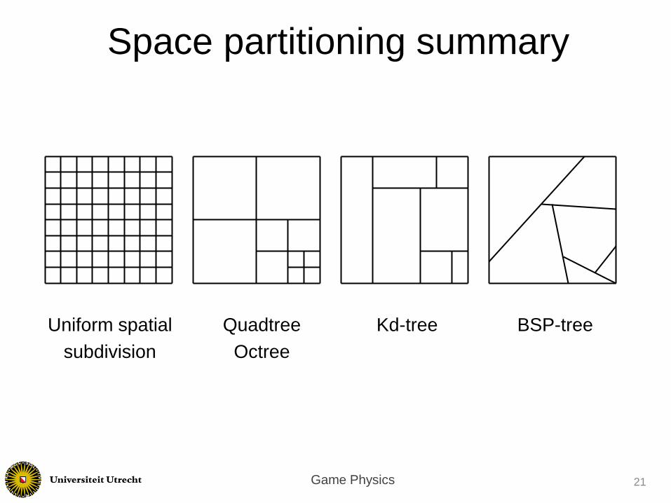
Space partitioning

Game Physics
• An octree is a tree data structure in which each
node has exactly eight children
• Partition the space in eight cubes (called octants)
of equal volume along the dimensions of the space
18
Octree

Game Physics
• A kd-tree (k-dimensional) is a binary tree where
every node is alternately associated with one of
the k-dimensions
• Usually the median hyperplane is chosen at each
node
19
Kd-tree

Game Physics
• Binary space partitioning (BSP) creates BSP trees
• Hyperplanes recursively partition space into two
volumes but the planes can have any orientation
• Hyperplanes are usually defined by polygons in
the scene
20
Binary space partitioning
A
B
1
1
2
2
3
3
PART
1
PART
2
PART 3
PART 6
PART
4 PART
5
PART 1
A1
A2
A3
A4
B1
B2
B3
PART 2
PART 3
PART 4
PART 5
PART 6 B
A
4
Game Physics
Uniform spatial
subdivision
21
Space partitioning summary
Quadtree
Octree
Kd-tree BSP-tree

Mid phase

Game Physics
• You can imagine representing different objects with
different primitives according to their original
geometry
– A simple convex object => convex hull
– A spherical object like a ball => bounding sphere
– A body part => bounding capsule
– A box sliding on the floor => AABB
– A box-like object that can translate and rotate => OBB
• Ideally you have to implement detection algorithms
for every possible combination of primitives
– Some are easier to implement than others
23
Collision between primitives

Game Physics
• For two spheres 𝐴 and 𝐵 to intersect, the distance
between their centers 𝑐𝐴 and 𝑐𝐵 should be smaller
than the sum of their radii 𝑟𝐴 and 𝑟𝐵
𝐴 ∩ 𝐵 ≠ ∅ ⇔ 𝑐𝐴 − 𝑐𝐵 ≤ 𝑟𝐴 + 𝑟𝐵
• Distance between two non-intersecting spheres 𝑑 𝐴, 𝐵 = max 𝑐𝐴 − 𝑐𝐵 − 𝑟𝐴 + 𝑟𝐵 , 0
• Penetration depth of two intersecting spheres
𝑝 𝐴, 𝐵 = max 𝑟𝐴 + 𝑟𝐵 − 𝑐𝐴 − 𝑐𝐵 , 0
24
Sphere-Sphere

Game Physics
• Project the boxes onto the axes, you will obtain
two/three intervals per box, the two boxes collide if
the intervals overlap
25
AABB-AABB
A
B
A
B

Game Physics
𝐴 ∩ 𝐵 = ∅ ⇔ 𝑥𝑚𝑎𝑥𝐴
< 𝑥𝑚𝑖𝑛𝐵∨ 𝑦𝑚𝑎𝑥𝐴
< 𝑦𝑚𝑖𝑛𝐵∨
𝑥𝑚𝑖𝑛𝐴> 𝑥𝑚𝑎𝑥𝐵
∨ 𝑦𝑚𝑖𝑛𝐴> 𝑦𝑚𝑎𝑥𝐵
26
AABB-AABB
A
B
𝑥
𝑦
𝑥𝑚𝑖𝑛𝐴 𝑥𝑚𝑎𝑥𝐴
𝑥𝑚𝑖𝑛𝐵 𝑥𝑚𝑎𝑥𝐵
𝑦𝑚𝑖𝑛𝐵
𝑦𝑚𝑖𝑛𝐴
𝑦𝑚𝑎𝑥𝐵
𝑦𝑚𝑎𝑥𝐴

Game Physics 27
Separating Axis Theorem
• Given two convex shapes, if we can find an axis
along which the projections of the two shapes do
not overlap, then the shapes do not collide

Game Physics
• In 2D, each of these potential separating axes is
perpendicular to one of the edges of each shape
– We solve our 2D overlap query using a series of 1D
queries
– If we find an axis along which the objects do not overlap,
we don't have to continue testing the rest of the axes,
we know that the objects don't overlap
• As in a game it is more likely for two objects
to not overlap, it speeds up calculations
28
Separating Axis Theorem

Game Physics
• For AABB-AABB it is easy to apply as the possible
separating axes on which we have to project the
object are the main axes
• Equivalent to our previous collision checking of
overlap of intervals
29
Separating Axis Theorem

Game Physics
• For non-axis-aligned shapes, we have to project
our objects on the axes perpendicular to the edges
Box-Polygon Box-Curve Circle-Polygon
30
Separating Axis Theorem

Game Physics
• Several variants exist but all first sort then prune
• Objects are defined with their AABB
• 2 objects overlap if and only if their projections on
the x, y and z coordinate axes overlap
– The projections give 3 [min,max] intervals
– The min and max are stored in 3 sorted structures
– Scan the objects in increasing order of min
– Detect possible overlapping pair when min of an object
is smaller than max of another
– Combine the three results (AND condition to overlap)
31
Sweep and prune algorithm

Game Physics 32
Sweep and prune algorithm
x, y or z axis
A
B
C
D
CurrentObjects
CandidatePairs
[C]
[CA] [BC,BA] [DA]
[C,A] [C,A,B] [A,B]
=
[CA,BC,BA,DA]
[A] [] [A,D] [A]
∪ ∪
[]

Game Physics
• Looking at uncorrelated sequences of positions is
not enough
• Our objects are in motion and we need to know
when and where they collide
– as we want to react to the collision e.g. bouncing
33
The time issue
At 𝑡
At 𝑡 + ∆𝑡

Game Physics
• Collision in-between steps can lead to tunneling
– Objects pass through each other
• They did not collide at 𝑡 and do not collide either at 𝑡 + ∆𝑡
• But they did collide somewhere in between
– Lead to false negatives
• Tunneling is a serious issue in gameplay
– Players getting to places they should not
– Projectiles passing through characters and walls
– Impossibility for the player to trigger actions on contact
events
34
Tunneling

Game Physics 35
Tunneling

Game Physics
• Small objects tunnel more easily
• Fast moving objects tunnel more easily
36
Tunneling

Game Physics
• Possible solutions
– Minimum size requirement?
• Fast object still tunnel
– Maximum speed limit?
• Small and fast objects not allowed (e.g. bullets...)
– Smaller time step?
• Essentially the same as speed limit
• We need another approach to the solution
37
Tunneling

Game Physics
• Bounds enclosing the motion of the shape
– In the time interval ∆𝑡, the linear motion of the shape is
enclosed
– Again, convex bounds are used, so the movement
bounds are themselves primitive shapes
38
Movement bounds

Game Physics
• Sphere
39
Movement bounds
• AABB
• OBB

Game Physics
• If movement bounds do not collide, there is no
collision
• If movement bounds collide, there is possibly a
collision
40
Movement bounds

Game Physics
• As primitive based movement bounds do not have
a really good fit, we can use swept bounds
– More accurate, but more costly to calculate collisions
• A swept bound (or swept shape) is constructed
from the union of all surfaces (volumes) of a shape
under a transformation
– we use the affine transformation from 𝑡 to t + ∆𝑡
41
Swept bounds

Game Physics
• Swept sphere capsule
• Swept AABB convex poly
• Swept triangle convex poly
• Swept convex poly convex poly
42
Swept bounds

Narrow phase

Game Physics
• This algorithm effectively determines the
intersection between polyhedra by computing the
Euclidean distance between them
• Based on the property that the distance is the
same as the shortest distance between their
Minkowski difference and the origin
• Two new problems
– Calculate the Minkowski difference between two objects
– Calculate its distance to the origin (i.e. coordinate of the
closest point to the origin)
44
GJK algorithm

Game Physics
• The Minkowski difference 𝐴 ⊖ 𝐵 = 𝐴⨁(−𝐵) is
obtained by adding 𝐴 to the reflection of 𝐵 about
the origin
• Addition here means the swept bound of 𝐵 using 𝐴
• If 𝐴 and 𝐵 collide, 𝐴 ⊖ 𝐵 contains the origin
45
Minkowski difference

Game Physics
• To calculate the shortest distance to the origin, the following algorithm is used 1. Initialize the simplex set 𝑄 with up to 𝑑 + 1 points from
the Minkowski difference object 𝐶
2. If the origin is in the convex hull 𝐶𝐻(𝑄), then stop (collision detected)
3. Compute the point 𝑃 of minimum norm of 𝐶𝐻(𝑄)
4. Reduce 𝑄 to the smallest subset 𝑄′ of 𝑄 such that 𝑃 ∈ 𝐶𝐻(𝑄′)
5. Let 𝑉 = 𝑆𝑐(−𝑃) be a supporting point in direction −𝑃
6. If 𝑉 is no more extreme than 𝑃 in direction −𝑃, then return 𝑃
7. Add 𝑉 to 𝑄 and go to step 2
46
GJK algorithm

Game Physics
• Imagine the following Minkowski difference object
𝐶 and origin 𝑂
47
GJK algorithm example
𝐶
𝑂

Game Physics
1. Initialize the simplex set 𝑄 with up to 𝑑+1 points
from the Minkowski difference object 𝐶
48
GJK algorithm example
0-simplex 1-simplex 2-simplex 3-simplex
simplex

Game Physics
1. Initialize the simplex set 𝑄 with up to 𝑑+1 points
from the Minkowski difference object 𝐶
49
GJK algorithm example
𝐶
𝑂
𝑄 = {𝑄0, 𝑄1, 𝑄2}
𝑄0
𝑄2
𝑄1

Game Physics
2. If the origin is in the convex hull 𝐶𝐻(𝑄), then stop
(collision detected)
50
GJK algorithm example
𝐶
𝑂
𝑄 = {𝑄0, 𝑄1, 𝑄2}
𝑄0
𝑄2
𝑄1

Game Physics
3. Compute the point 𝑃 of minimum norm of the
convex hull 𝐶𝐻(𝑄)
51
GJK algorithm example
𝐶
𝑂
𝑄 = {𝑄0, 𝑄1, 𝑄2}
𝑄0
𝑄2
𝑄1
𝑃

Game Physics
4. Reduce 𝑄 to the smallest subset 𝑄′ of 𝑄 such that
𝑃 ∈ 𝐶𝐻(𝑄′)
52
GJK algorithm example
𝑂
𝑄 = {𝑄1, 𝑄2}
𝑄2
𝑄1
𝑃

Game Physics
5. Let 𝑉 = 𝑆𝑐(−𝑃) be a supporting point in direction
− 𝑃
53
GJK algorithm example
Supporting point 𝑉 for a direction 𝑑 returned by support mapping function 𝑆𝑐(𝑑)
𝑉 𝑉
𝑑
𝐶 𝐶

Game Physics
5. Let 𝑉 = 𝑆𝑐(−𝑃) be a supporting point in direction
− 𝑃. Let’s call it 𝑉1.
54
GJK algorithm example
𝑂
𝑄 = {𝑄1, 𝑄2}
𝑄2
𝑄1
𝑃
𝑉1 = 𝑆𝑐(−𝑃)

Game Physics
6. If 𝑉 is no more extreme than 𝑃 in direction −𝑃,
then return 𝑃
7. Add 𝑉 to 𝑄 and go to step 2
55
GJK algorithm example
𝑂
𝑄 = {𝑄1, 𝑄2, 𝑉1}
𝑄2
𝑄1
𝑉1
𝑃

Game Physics
2. If the origin is in the convex hull 𝐶𝐻(𝑄), then stop
(collision detected)
56
GJK algorithm example
𝑂
𝑄 = {𝑄1, 𝑄2, 𝑉1}
𝑄2
𝑄1
𝑉1

Game Physics
3. Compute the point 𝑃 of minimum norm of the
convex hull 𝐶𝐻(𝑄)
57
GJK algorithm example
𝑂
𝑄 = {𝑄1, 𝑄2, 𝑉1}
𝑄2
𝑄1
𝑉1 𝑃

Game Physics
4. Reduce 𝑄 to the smallest subset 𝑄′ of 𝑄 such that
𝑃 ∈ 𝐶𝐻(𝑄′)
58
GJK algorithm example
𝑂
𝑄 = {𝑄2, 𝑉1}
𝑄2
𝑃 𝑉1

Game Physics
5. Let 𝑉 = 𝑆𝑐(−𝑃) be a supporting point in direction
− 𝑃. Let’s call it 𝑉2.
59
GJK algorithm example
𝑂
𝑄2 = 𝑆𝑐 𝑃 = 𝑉2
𝑄 = {𝑄2, 𝑉1} 𝑃
𝑉1

Game Physics
6. If 𝑉 is no more extreme than 𝑃 in direction −𝑃,
then return 𝑃
60
GJK algorithm example
𝑂
𝑄2 = 𝑉2
𝑄 = {𝑄2, 𝑉1} 𝑃
𝑉1
DONE!
Distance is 𝑃

Game Physics
• In step 5 we had to find the supporting point of 𝐶 in
the direction −𝑃
• It was intuitive an our example but how can we
automatically calculate that point in any given
situation?
– we need the actual definition of a supporting point
61
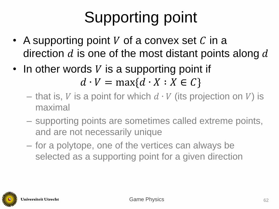
Supporting point
Game Physics
• A supporting point 𝑉 of a convex set 𝐶 in a
direction 𝑑 is one of the most distant points along 𝑑
• In other words 𝑉 is a supporting point if
𝑑 ∙ 𝑉 = max{𝑑 ∙ 𝑋 ∶ 𝑋 ∈ 𝐶}
– that is, 𝑉 is a point for which 𝑑 ∙ 𝑉 (its projection on 𝑉) is
maximal
– supporting points are sometimes called extreme points,
and are not necessarily unique
– for a polytope, one of the vertices can always be
selected as a supporting point for a given direction
62
Supporting point

Game Physics
• A support mapping 𝑆𝐶(𝑑) is a function that maps
the direction 𝑑 into a supporting point of 𝐶
• For simple convex shapes, support mappings can
be given in closed form
– Sphere centered at 𝑐 of radius 𝑟
𝑆𝐶 𝑑 = 𝑐 + 𝑟𝑑
𝑑
– AABB centered at 𝑐 with size 2𝑒𝑥 × 2𝑒𝑦 × 2𝑒𝑧
𝑆𝐶 𝑑 = 𝑐 + 𝑠𝑖𝑔𝑛 𝑑𝑥 𝑒𝑥 , 𝑠𝑖𝑔𝑛 𝑑𝑦 𝑒𝑦, 𝑠𝑖𝑔𝑛 𝑑𝑧 𝑒𝑧
where 𝑠𝑖𝑔𝑛 𝛼 = −1 if 𝛼 < 0 and 1 otherwise
– Formulas exist for cylinder, cone etc.
63
Support mapping

Game Physics
• Convex shapes of higher complexity require the
support mapping function to determine a support point
using numerical methods
• For a polytope of 𝑛 vertices, a supporting vertex is
trivially found in 𝑂(𝑛) by searching over all vertices
• A greedy algorithm can be used to optimize the search
by exploring the polytope through a simple hill-climbing
algorithm (using the 𝑑 ∙ 𝑋𝑖 values)
– with extra optimizations we can design an algorithm in
𝑂(log 𝑛)
– we can also use frame coherency for determining the starting
point, and then in practice we observe a performance almost
insensitive to the complexity of the objects!
64
Support mapping 6.1

Game Physics
• Remember the collision detection algorithm
– Broad phase
• disregard pairs of objects that cannot collide
model and space partitioning
– Mid phase
• determine potentially colliding primitives
movement bounds
– Narrow phase
• determine exact contact between two shapes
Gilbert-Johnson-Keerthi algorithm
65
Collision detection algorithm

End of
Collision detection
Next
Collision resolution
Top Related