


Languages
Pages
Legal


Journal of Soft Computing in Civil Engineering 2-1 (2018) 01-17
journal homepage: http://www.jsoftcivil.com/
Fuzzy Vibration Suppression of a Smart Elastic Plate
using Graphical Computing Environment
A. D. Muradova, G. K. Tairidis and G. E. Stavroulakis*
School of Production Engineering and Management, Technical University of Crete, Chania, Greece
Corresponding author: [email protected]
ARTICLE INFO
ABSTRACT
Article history:
Received: 11 August 2017
Accepted: 28 September 2017
A nonlinear model for the vibration suppression of a smart
composite elastic plate using graphical representation
involving fuzzy control is presented. The plate follows the
von Kármán and Kirchhoff plate bending theories and the
oscillations are caused by external transversal loading forces,
which are applied directly on it. Two different control forces,
one continuous and one located at discrete points, are
considered. The mechanical model is spatially discretized by
using the time spectral Galerkin and collocation methods.
Our aim is to suppress vibrations through a simulation
process within a modern graphical computing environment.
Here we use MATLAB/SIMULINK, while other similar
packages can be used as well. The nonlinear controller is
designed, based on an application of a Mamdani-type fuzzy
inference system. A computational algorithm, proposed and
tested here is not only effective, but robust as well.
Furthermore, all elements of the study can be replaced or
extended, due to the flexibility of the used SIMULINK
environment.
Keywords:
Smart plate model,
Spatial discretization,
Fuzzy control,
Computational algorithm,
SIMULINK diagrams.
1. Introduction
Classical mathematical theories of control work well on linear systems. However, their
effectiveness depends on many restrictions. On the other hand nonlinear controllers, based on
fuzzy logic with built in smart computational methods can give a good description of a behaviour
of nonlinear structures and provide a nonlinear feedback. The details of comparison between the
classical control and fuzzy logic approach are discussed, among others, in the paper of Tairidis et
al. [1].
An active vibration control of smart elastic plates has been considered by many authors. An
active vibration control incorporating active piezoelectric actuator and self-learning control for a
flexible plate structure is described by Tavakolpour et al. [2]. In the paper of Fisco and Adeli [3]
2 A. Muradova et al./ Journal of Soft Computing in Civil Engineering 2-1 (2018) 01-17
hybrid control strategies, in particular active and semi-active vibration suppression are discussed.
A brief survey on industrial applications of fuzzy control in different fields of engineering is
given in the works of Precup and Hellendoorn [4]. The control systems are classified on three
groups, control systems with Mamdani fuzzy controllers, control systems with Takagi-Sugeno
fuzzy controllers, and adaptive and predictive control systems. A review of active structural
control is done by Korkmaz in [5].
Here a vibration suppression of a smart plate is performed by the algorithm, involving
constructed model-diagrams of SIMULINK with the use of Mamdani FIS. In the paper [6] a
Newmark technique is applied for solving the system of linear ordinary differential equations
(ODEs), obtained after the spatial discretization of the model. In this paper, we use a graphical
representation for solving linear and nonlinear ODEs. The numerical simulation is implemented
with the use of model-diagrams of SIMULINK. That allows easily and quickly suppressing
vibrations of the plate and improves the presentation of the results. We can also include a
Sugeno-type fuzzy inference system in the complete model-diagram for the linear model, i.e., the
new approach provides flexibility of choosing a controller. Besides, we have tested a collocation
method, which provides an opportunity to locate control forces at discrete points of the plate.
The proposed algorithm allows effective suppression of the Fourier coefficients, which actually
display characteristics of displacement, velocity and Airy's stress function (in other words,
general displacement, velocity and Airy's function) of the plate. After computing the coefficients
we can easily calculate the displacement and velocity at each point of the plate.
Active fuzzy control is a suitable tool for the systematic development of nonlinear control
strategies and can be fine-tuned if no experience exists in the behaviour of considered body
(structure) or if one designs more complicated control schemes, (e.g. [7-11]). Similar approaches
for active vibration control of a simply supported rectangular plate using fuzzy logic rules are
discussed in the paper of Shirazi et al. [11]. The results have been compared with the classical
proportional integral derivative (PID) controller.
The present paper is organized as follows. Section 2 focuses on a formulation of the nonlinear
dynamic mechanical model, and set up initial and boundary conditions. In Section 3 the spatially
discretized model is presented. In both cases (Galerkin' projections and collocation approach) the
result of discretization is a system of second order nonlinear ordinary differential equations of
motion. In Section 4 an algorithm for vibration suppression is introduced. The algorithm
involves, constructed model-diagrams with composed ``S-Function'' of SIMULINK. A numerical
example using Galerkin's projections and the developed algorithm is presented. Section 5 is
devoted to a state space representation of the linearized spatially discretized problem. We
reformulate above mentioned algorithm for the linear model. Instead of the ``S-Function'' a
``State-Space'' block mode' is activated. The implementation of the collocation method for the
linear case is illustrated in a numerical example. The main results are reported in Section 6.

A. Muradova et al./ Journal of Soft Computing in Civil Engineering 2-1 (2018) 01-17 3
2. Formulation of the Problem
Governing equations. A nonlinear mathematical model describing the bending vibrations of an
isotropic, homogeneous elastic plate in the presence of active control, and allowance for the
rotational inertia of the plate elements and viscous damping is written as
𝐿1(𝑤, 𝜓) ≡ 𝜌ℎ𝑤𝑡𝑡 − 𝜌ℎ3
12Δ𝑤𝑡𝑡 + ℎ𝑐𝑤𝑡 + 𝐷Δ2𝑤 − ℎ[𝑤, 𝜓] = [𝑄] + [𝑍], (1)
𝐿2(𝑤, 𝜓) ≡ Δ2𝜓 −𝐸
2[𝑤, 𝑤] = 0, (𝑡, 𝑥, 𝑦) ∈ Ω. (2)
Here the following notations are used:
[𝑤, 𝜓] = 𝜕11𝑤𝜕22𝜓 + 𝜕11𝜓𝜕22𝑤 − 2𝜕12𝑤𝜕12𝜓 (Monge-Ampére’s form).
o 𝑤 is the deflection (displacement) of the plate.
o 𝜓(𝑡, 𝑥, 𝑦) is the Airy stress potential describing internal stresses, which appear due to the
deformation of the plate (e.g., [12-14]).
o Ω = (0, 𝑇] × 𝐺, where 𝑇 is the final time and 𝐺 = (0, 𝑙1) × (0, 𝑙2) is the shape of the plate (𝑙1
and 𝑙2 are the lengths of the sides of the plate).
o 𝜌 is the density of the material.
o ℎ is the thickness of the plate.
o 𝑐 is the viscous damping coefficient.
o 𝐷 is the flexural rigidity of the plate.
o [𝑄] are the external transversal loading forces.
o [𝑍] are the control forces.
The equations Eq.1, Eq.2 are extensions of the nonlinear von Kármán plate model for large
deflections ([13], [14] etc.) on a control case. The plate is subjected to external transversal
disturbances and generalized control forces, produced, for example, by electromechanical
coupling effects.
For the Galerkin’s projections it is required that 𝑤, 𝜓 ∈ 𝐶2(0, 𝑇; 𝑊2,2(𝐺)), (𝑊2,2 is the Sobolev
space). For the collocation method it is required that 𝑤, 𝜓 ∈ 𝐶2(0, 𝑇; 𝐶2(𝐺)) ∪ 𝐶(0, 𝑇; 𝐶4(𝐺)).
Regarding the loading forces we consider [𝑄] as a function of (𝑡, 𝑥, 𝑦) or as a discrete function
only of 𝑡, defined at some collocation points of the plate. We assume the same for the control
forces [𝑍]. When [𝑍] is supposed to be a function of (𝑡, 𝑥, 𝑦), it is expanded into double Fourier's
series and we use the time spectral Galerkin method for spatial discretization of 𝐿1, 𝐿2. The
suppression of vibrations is done through the control of the Fourier coefficients. Here we also
introduce a new approach, by considering a time-discrete type of control force [𝑍], located at
some discrete-collocation points of the plate, which may be different from the points where
external forces are applied.
Initial and boundary conditions. For the displacement and velocity at the initial time we assume
𝑤(0, 𝑥, 𝑦) = 𝑢(𝑥, 𝑦), 𝑤𝑡(0, 𝑥, 𝑦) = 𝜈(𝑥, 𝑦) in 𝐺,

4 A. Muradova et al./ Journal of Soft Computing in Civil Engineering 2-1 (2018) 01-17
where the functions 𝑢, 𝜈 belong to the quadratically integrable function space 𝐿2(𝐺).
Regarding the boundary conditions we consider simply supported, partially and totally clamped
plates (see [15], [16]).
3. Spatial discretization of the problem Eq.1, Eq.2
3.1. Time spectral expansions.
An approximate analytical solution of Eq.1, Eq.2 in the form of partial sums of double Fourier's
series with the time-dependent coefficients ([15]) reads
𝑊𝑁(𝑡, 𝑥, 𝑦) = ∑ 𝑤𝑁𝑖𝑗(𝑡)
𝑁
𝑖,𝑗=1
ω𝑖𝑗(x, y), 𝑊𝑁(𝑡, 𝑥, 𝑦) = ∑ 𝑤𝑡,𝑁𝑖𝑗 (𝑡)
𝑁
𝑖,𝑗=1
ω𝑖𝑗(x, y), (3)
𝛹𝑁(𝑡, 𝑥, 𝑦) = ∑ 𝜓𝑁𝑖𝑗(𝑡)
𝑁
𝑖,𝑗=1
𝜑𝑖𝑗(x, y), (𝑡 > 0), (4)
where the global basis functions 𝜔𝑖𝑗 are chosen to match the boundary conditions [15]. For the
initial conditions we have
𝑊𝑁(0, 𝑥, 𝑦) = 𝑢𝑁(𝑥, 𝑦) = ∑ 𝑤𝑁𝑖𝑗(0)
𝑁
𝑖,𝑗=1
φij(x, y), (5)
𝑊𝑡,𝑁(0, 𝑥, 𝑦) = 𝑣𝑁(𝑥, 𝑦) = ∑ 𝑤𝑡,𝑁𝑖𝑗 (0)
𝑁
𝑖,𝑗=1
σij(x, y), (6)
where 𝜑𝑖𝑗 and 𝜎𝑖𝑗 are the bases. It is assumed 𝜑𝑖𝑗 = 𝜎𝑖𝑗 = 𝜔𝑖𝑗. In case when [𝑍] is a function of
(𝑡, 𝑥, 𝑦) we expand it into double Fourier series with the basic functions 𝜔𝑖𝑗, i.e.,
[𝑍] ≡ 𝑍𝑁(𝑡, 𝑥, 𝑦) = ∑ 𝑧𝑁𝑖𝑗(𝑡)
𝑁
𝑖,𝑗=1
𝜔𝑖𝑗(𝑥, 𝑦). (7)
According to the two algorithms, introduced first for the linear case in [6], and extended for the
nonlinear case in [16] the vibration suppression can be performed by means of the control
function 𝑍 or the Fourier coefficients 𝑧𝑁𝑖𝑗
(𝑡). In the present paper we study the second case.
3.2. Galerkin's projections.
Let the external loading force [𝑄] is a quadratically integrable function 𝑄, i.e., 𝑄 ∈ 𝐿2(𝐺) and
[𝑍] is defined as Eq.7. Introducing the inner product in 𝐿2 - space and applying Galerkin's
projections to Eq.1, Eq.2 yields
⟨𝐿1(𝑊𝑁, 𝛹𝑁 ), 𝜔𝑚𝑛⟩ = ⟨𝑄, 𝜔𝑚𝑛⟩ + ⟨𝑍𝑁, 𝜔𝑚𝑛⟩,
⟨𝐿2(𝑊𝑁, 𝛹𝑁 ), 𝜔𝑚𝑛⟩ = 0, 𝑚, 𝑛 = 1,2, … , 𝑁.

A. Muradova et al./ Journal of Soft Computing in Civil Engineering 2-1 (2018) 01-17 5
Hence
𝐌�̈�𝑁(𝑡) + 𝐂�̇�𝑁(𝑡) + 𝐊1𝐰𝑁(𝑡) = 𝐀1,𝑁(𝐰𝑁(𝑡), 𝛙𝑁(𝑡)) + 𝐏𝐪𝑁(𝑡) + 𝐅𝐳𝑁(𝑡), (8)
𝐊2𝐰𝑁(𝑡) = 𝐀2,𝑁(𝐰𝑁(𝑡), 𝐰𝑁(𝑡)), (9)
where 𝐰𝑁(𝑡), 𝛙𝑁(𝑡) are the vectors with the components which are the Fourier coefficients for
the displacement Eq.3, and the Airy stress function Eq.4, respectively. We call them
characteristics of the displacement and the Airy stress function, respectively. Further, 𝐌 =
𝜌ℎ(𝐇 + (ℎ2/12)𝐁) is the mass matrix (𝐁 is the approximation of the Laplacian), 𝐂 is the
viscous damping matrix, 𝐊1 is the stiffness matrix. The matrices 𝐊1, 𝐊2 are the result of
approximation of the biharmonic operator and 𝐀1,𝑁, 𝐀2,𝑁 are nonlinear approximations of the
Monge-Ampère forms. Finally, P and F are the matrices and 𝐪𝑁, 𝐳𝑁 are the vectors, obtained
after the approximations of the external exciting pressure and control forces, respectively. The
operators H, B, P and F take different forms depending on the boundary conditions. The
description of the above defined operators are given in [15]. Substituting Eq.9 into Eq.8 we
obtain
𝐌�̈�𝑁 + 𝐂�̇�𝑁 + 𝐊1𝐰𝑁 = 𝐀1,𝑁 (𝐰𝑁, 𝐊2−1𝐀2,𝑁(𝐰𝑁, 𝐰𝑁)) + 𝐏𝐪𝑁 + 𝐅𝐳𝑁. (10)
For the components from Eq.10 we have
(𝐌�̈�𝑁)𝑚𝑛 + (𝐂�̇�𝑁)𝑚𝑛 + (𝐊1𝐰𝑁)𝑚𝑛 = (𝐀1,𝑁 (𝐰𝑁, 𝐊2−1𝐀2,𝑁(𝐰𝑁, 𝐰𝑁)))
𝑚𝑛
+(𝐏𝐪𝑁)𝑚𝑛 + (𝐅𝐳𝑁)𝑚𝑛, 𝑚, 𝑛 = 1,2, … , 𝑁 . (11)
For the initial conditions Eq.5, Eq.6 after applying Galerkin's projections we obtain
(𝐔𝐰𝑁(0))𝑚𝑛
= ⟨𝑢𝑁(𝑥, 𝑦), 𝜔𝑚𝑛⟩,
(𝐕𝐰𝑁(0))𝑚𝑛
= ⟨𝑣𝑁(𝑥, 𝑦), 𝜔𝑚𝑛⟩, 𝑚, 𝑛 = 1,2, … , 𝑁.
where 𝑢, 𝑣 are described in [15].
If the inputs for the fuzzy controller are 𝑤𝑁𝑚𝑛(𝑡) and �̇�𝑁
𝑚𝑛(𝑡) then the output is the control
𝑧𝑚𝑛(𝑡) for these coefficients.
3.3. Collocation approach.
Let us now consider the collocation points (𝑥𝑘 , 𝑦𝑙), {(𝑥𝑘, 𝑦𝑙), 0 < 𝑥𝑘 < 𝑙1, 0 < 𝑦𝑙 < 𝑙2, 𝑘, 𝑙 =
1,2, . . . , 𝑁} on the spatial domain G for the system Eq.1, Eq. 2. Suppose that [𝑄] is the function
of time defined at some or all collocation points. Similary let the control forces [𝑍] be put at
some collocation points, which may coincide with the points of application of the loading
pressure. We find the solution of Eq.1, Eq.2 in the form Eq.3, Eq.4 when 𝑊𝑁 and 𝛹𝑁 satisfy the
equations Eq.1, Eq.2 at the collocation points, i.e.

6 A. Muradova et al./ Journal of Soft Computing in Civil Engineering 2-1 (2018) 01-17
𝐿1(𝑊𝑁, 𝛹𝑁)|(𝑥=𝑥𝑘,𝑦=𝑦𝑙 ) = [𝑄]|(𝑥=𝑥𝑘,𝑦=𝑦𝑙 ) + [𝑍]|(𝑥=𝑥𝑘,𝑦=𝑦𝑙 ), (12)
𝐿2(𝑊𝑁, 𝛹𝑁)|(𝑥=𝑥𝑘,𝑦=𝑦𝑙 ) = 0, 𝑘, 𝑙 = 1,2, … , 𝑁. (13)
Supposing that control forces are located at every or some collocation points, from Eq.12 and
Eq.13 we obtain a system of nonlinear ordinary differential equations of motion with respect to
𝑤𝑁𝑚𝑛 and 𝜓𝑁
𝑚𝑛, similar with the previous one Eq.10
𝐌�̈�𝑁 + 𝐂�̇�𝑁 + 𝐊1𝐰𝑁 = 𝐀1,𝑁 (𝐰𝑁, 𝐊2
−1𝐀2,𝑁(𝐰𝑁, 𝐰𝑁)) + 𝐪 + 𝐳 , (14)
and similar to Eq.11
(𝐌�̈�𝑁)𝑘𝑙
+ (𝐂�̇�𝑁)𝑘𝑙
+ (𝐊1𝐰𝑁)𝑘𝑙
= (𝐀1,𝑁 (𝐰𝑁, 𝐊2
−1𝐀2,𝑁(𝐰𝑁, 𝐰𝑁)))
𝑘𝑙
+ 𝐪𝑘𝑙
+ 𝐳𝑘𝑙 ,
𝑘, 𝑙 = 1,2, … , 𝑁, (15)
where 𝐌 is the mass matrix, 𝐂 is the damping matrix and 𝐊1 is the stiffness matrix. The
elements of the matrices are determined through computations of the partial derivatives of 𝑊𝑁
and Ψ𝑁 (see Eq.3, Eq.4) with respect to the spatial variables 𝑥, 𝑦 at the collocation points. The
elements of the matrices 𝐌 , 𝐂 , 𝐊1 and 𝐊2 can be easily calculated. They are the values of the
basic functions 𝜔𝑖𝑗(𝑥𝑘, 𝑦𝑙). Analogously, the nonlinear parts are defined.
Furthermore, in Eq.14 𝐪 is a vector with components 𝑞𝑘𝑙
, the values of the time-discrete forces at
some collocation points (𝑥𝑘, 𝑦𝑙), 𝑘, 𝑙 = 𝑁1, 𝑁1 + 1, . . . , 𝑁2 and 𝐳 is the vector with components
𝑧𝑘𝑙, the values of the control forces at some collocation points (𝑥𝑘, 𝑦𝑙), 𝑘, 𝑙 = 𝑀1, 𝑀1 +
1, . . . , 𝑀2. . The collocation points where the external loading forces are applied are called
loading points and the points where we put/locate the control are called control points. In case
𝑁1 ≡ 𝑀1 ≤ 𝑁 and 𝑁2 ≡ 𝑀2 ≤ 𝑁 the loading points coincide with the control points.
Obviously, we can also deal with free collocation points, where the external and control forces
are absent. At these points the values of the external and control forces are supposed to be zero.
The advantage of the collocation method over the Galerkin's projections is that we do not need to
take the inner products, and we can consider external loading disturbances at the discrete points
and locate the control forces at the places of (all or some) collocation points in the proper way.
Inversely, the collocation points can be considered at the best positions for the control, i.e. the
collocation points are chosen in order to provide optimal suppressions of vibrations of the plate.
A disadvantage of the collocation method is that one may lose an accuracy of the approximate
solution between the collocation points, and the obtained mass, damping and stiffness matrices
are not so sparse as in case of Galerkin's projections.
For the initial conditions from Eq.5, Eq.6 we have
∑ 𝑤𝑁𝑖𝑗
𝑁
𝑖,𝑗=1
(0)𝜔𝑖𝑗(𝑥, 𝑦) = 𝑢𝑁(𝑥𝑘 , 𝑦𝑙), ∑ 𝑤𝑡,𝑁𝑖𝑗
𝑁
𝑖,𝑗=1
(0)𝜔𝑖𝑗(𝑥, 𝑦) = 𝑣𝑁(𝑥𝑘 , 𝑦𝑙),
A. Muradova et al./ Journal of Soft Computing in Civil Engineering 2-1 (2018) 01-17 7
3.4. State-space representation
Let us now suppose 𝐯1 ≡ 𝐰, 𝐯2 ≡ �̇� (here and below the index N is omitted for the
convenience). Then from Eq.10 we obtain
�̇�1 = 𝐯2
𝐌𝐯2 + 𝐂𝐯2 + 𝐊1𝐯1 = 𝐀1,𝑁 (𝐯1, 𝐊2−1𝐀2,𝑁(𝐯1, 𝐯1)) + 𝐏𝐪𝑁 + 𝐅𝐳𝑁
or
�̇�1 = 𝐯2,
𝐯2 = 𝐌−1 [−𝐂𝐯2 − 𝐊1𝐯1 + 𝐏𝐪𝑁 + 𝐅𝐳𝑁 + 𝐀1,𝑁 (𝐯1, 𝐊2−1𝐀2,𝑁(𝐯1, 𝐯1))]. (16)
Analogously, for the model Eq.14
�̇�1 = 𝐯2,
𝐯2 = 𝐌−1
[−𝐂𝐯2 − 𝐊1𝐯1 + 𝐪 + 𝐳 + 𝐀1,𝑁 (𝐯1, 𝐊2
−1𝐀2,𝑁(𝐯1, 𝐯1))]. (17)
4. Algorithm of suppression of the Fourier coefficients and their derivatives
The use of model-diagrams of SIMULINK allows us quickly and effectively calculate the
suppressed Fourier coefficients in the expansions Eq.3, Eq.4. After that one can easily calculate
the suppressed vibrations at each point of the plate.
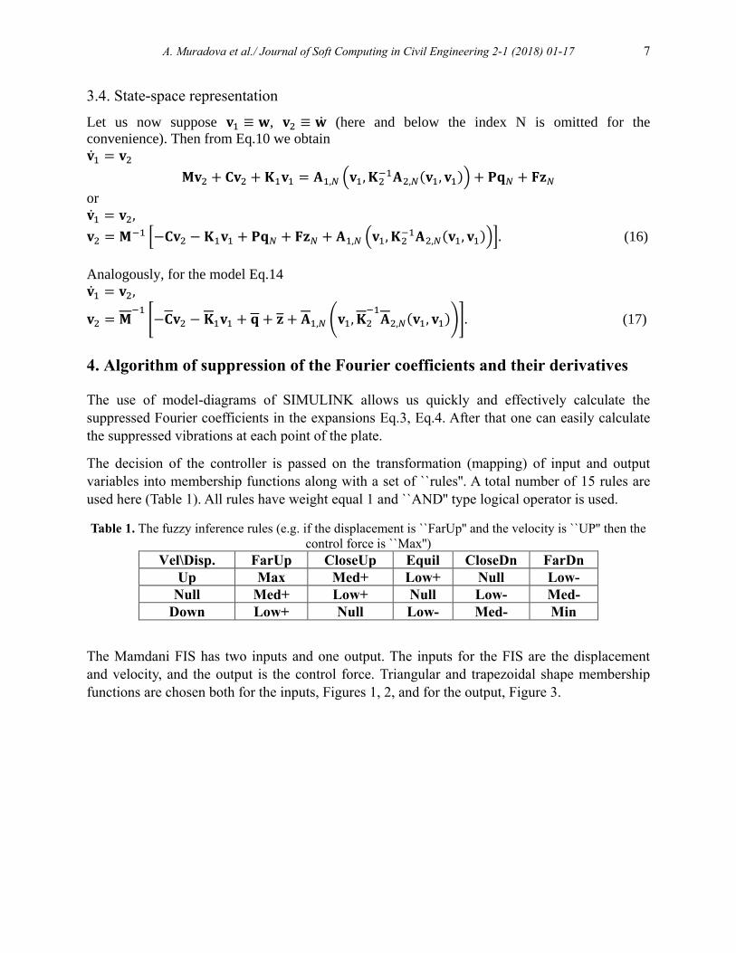
The decision of the controller is passed on the transformation (mapping) of input and output
variables into membership functions along with a set of ``rules''. A total number of 15 rules are
used here (Table 1). All rules have weight equal 1 and ``AND'' type logical operator is used.
Table 1. The fuzzy inference rules (e.g. if the displacement is ``FarUp'' and the velocity is ``UP'' then the
control force is ``Max'')
Vel\Disp. FarUp CloseUp Equil CloseDn FarDn
Up Max Med+ Low+ Null Low-
Null Med+ Low+ Null Low- Med-
Down Low+ Null Low- Med- Min
The Mamdani FIS has two inputs and one output. The inputs for the FIS are the displacement
and velocity, and the output is the control force. Triangular and trapezoidal shape membership
functions are chosen both for the inputs, Figures 1, 2, and for the output, Figure 3.

8 A. Muradova et al./ Journal of Soft Computing in Civil Engineering 2-1 (2018) 01-17
Fig. 1. Membership functions for the input (displacement) of the fuzzy inference system.
Fig. 2. Membership functions for the input (velocity) of the fuzzy inference system.
A. Muradova et al./ Journal of Soft Computing in Civil Engineering 2-1 (2018) 01-17 9
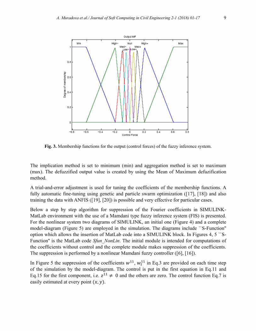
Fig. 3. Membership functions for the output (control forces) of the fuzzy inference system.
The implication method is set to minimum (min) and aggregation method is set to maximum
(max). The defuzzified output value is created by using the Mean of Maximum defuzification
method.
A trial-and-error adjustment is used for tuning the coefficients of the membership functions. A
fully automatic fine-tuning using genetic and particle swarm optimization ([17], [18]) and also
training the data with ANFIS ([19], [20]) is possible and very effective for particular cases.
Below a step by step algorithm for suppression of the Fourier coefficients in SIMULINK-
MatLab environment with the use of a Mamdani type fuzzy inference system (FIS) is presented.
For the nonlinear system two diagrams of SIMULINK, an initial one (Figure 4) and a complete
model-diagram (Figure 5) are employed in the simulation. The diagrams include ``S-Function''
option which allows the insertion of MatLab code into a SIMULINK block. In Figures 4, 5 ``S-
Function'' is the MatLab code Sfun_NonLin. The initial module is intended for computations of
the coefficients without control and the complete module makes suppression of the coefficients.
The suppression is performed by a nonlinear Mamdani fuzzy controller ([6], [16]).
In Figure 5 the suppression of the coefficients 𝑤11, 𝑤𝑡11 in Eq.3 are provided on each time step
of the simulation by the model-diagram. The control is put in the first equation in Eq.11 and
Eq.15 for the first component, i.e. 𝑧11 ≠ 0 and the others are zero. The control function Eq.7 is
easily estimated at every point (𝑥, 𝑦).
10 A. Muradova et al./ Journal of Soft Computing in Civil Engineering 2-1 (2018) 01-17
Algorithm for vibration suppression
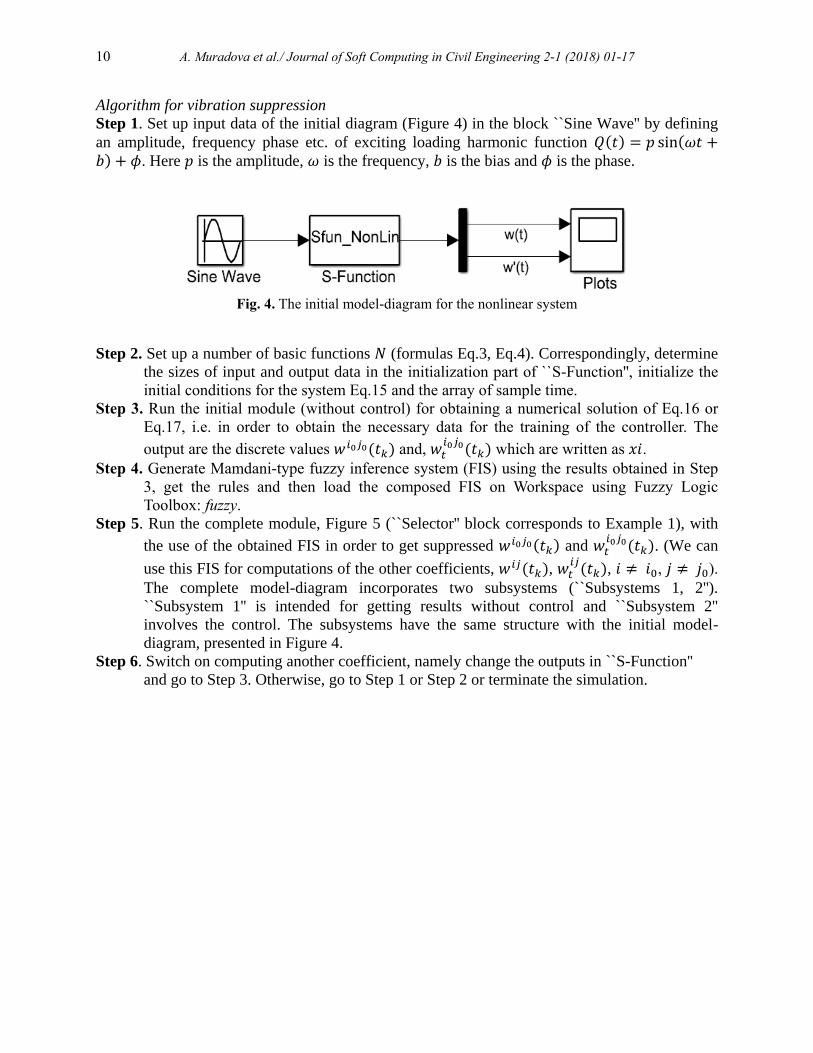
Step 1. Set up input data of the initial diagram (Figure 4) in the block ``Sine Wave'' by defining
an amplitude, frequency phase etc. of exciting loading harmonic function 𝑄(𝑡) = 𝑝 sin(𝜔𝑡 +𝑏) + 𝜙. Here 𝑝 is the amplitude, 𝜔 is the frequency, 𝑏 is the bias and 𝜙 is the phase.
Fig. 4. The initial model-diagram for the nonlinear system
Step 2. Set up a number of basic functions 𝑁 (formulas Eq.3, Eq.4). Correspondingly, determine
the sizes of input and output data in the initialization part of ``S-Function'', initialize the
initial conditions for the system Eq.15 and the array of sample time.
Step 3. Run the initial module (without control) for obtaining a numerical solution of Eq.16 or
Eq.17, i.e. in order to obtain the necessary data for the training of the controller. The
output are the discrete values 𝑤𝑖0𝑗0(𝑡𝑘) and, 𝑤𝑡𝑖0𝑗0(𝑡𝑘) which are written as 𝑥𝑖.
Step 4. Generate Mamdani-type fuzzy inference system (FIS) using the results obtained in Step
3, get the rules and then load the composed FIS on Workspace using Fuzzy Logic
Toolbox: fuzzy.
Step 5. Run the complete module, Figure 5 (``Selector'' block corresponds to Example 1), with
the use of the obtained FIS in order to get suppressed 𝑤𝑖0𝑗0(𝑡𝑘) and 𝑤𝑡𝑖0𝑗0(𝑡𝑘). (We can
use this FIS for computations of the other coefficients, 𝑤𝑖𝑗(𝑡𝑘), 𝑤𝑡𝑖𝑗
(𝑡𝑘), 𝑖 ≠ 𝑖0, 𝑗 ≠ 𝑗0).
The complete model-diagram incorporates two subsystems (``Subsystems 1, 2'').
``Subsystem 1'' is intended for getting results without control and ``Subsystem 2''
involves the control. The subsystems have the same structure with the initial model-
diagram, presented in Figure 4.
Step 6. Switch on computing another coefficient, namely change the outputs in ``S-Function''
and go to Step 3. Otherwise, go to Step 1 or Step 2 or terminate the simulation.

A. Muradova et al./ Journal of Soft Computing in Civil Engineering 2-1 (2018) 01-17 11
Fig. 5. The complete model-diagram.
In order to calculate the suppressed displacement 𝑊(𝑡𝑘, 𝑥, 𝑦) and suppressed velocity
𝑊𝑡(𝑡𝑘 , 𝑥, 𝑦) at any point (𝑥, 𝑦) of the plate at discrete time 𝑡 = 𝑡𝑘 we use the values of the
coefficients, obtained by the above given algorithm and substitute them into the analytical
expressions Eq.3. The coefficients 𝜓𝑁𝑖𝑗
(𝑡) in Eq.4 can be computed through the equations Eq.9 or
Eq.13. We can compute the coefficients as many as necessary in order to get more accurate
solution in sense of suppression of the displacement 𝑊(𝑡, 𝑥, 𝑦) and velocity 𝑊𝑡(𝑡, 𝑥, 𝑦) at each
point of the plate.
Below we consider an example of vibration suppressions of a simply supported plate by the
described above algorithm with the use of the time spectral (Galerkin) method, Section 3.
Example 1.
Let the external force be a harmonic exciting load, 𝑄(𝑡) = sin 10𝜋 𝑡 uniformly distributed on the
simply supported plate. Then 𝑝𝑚𝑛 = (𝑄, 𝜔𝑚𝑛) = (𝐏 𝐪𝑁)𝑚𝑛 = 8√𝑙1𝑙1/𝜋2𝑚𝑛. The amplitude in
the option for the ``Sine Wave'' block in Figures, 4, 5 is a vector P with 18 components. It is
defined as 𝐏 = (0, 𝑝11, 0, 𝑝12, 0, 𝑝13, 0, 𝑝21, 0, 𝑝22, 0, 𝑝23, 0, 𝑝31, 0, 𝑝32, 0, 𝑝33)𝑇. The control
forces are added only to the second component 𝑝11 , i.e. to the right hand side of the second
equation Eq.16. Thus, we have three ``Selector'' blocks: ``1 of 18'', ``2 of 18'' and ``3-18 of 18''.
The control forces are added in the ``Selector'' block ``2 of 18'', i.e. to the second component of
the vector 𝐏.
12 A. Muradova et al./ Journal of Soft Computing in Civil Engineering 2-1 (2018) 01-17
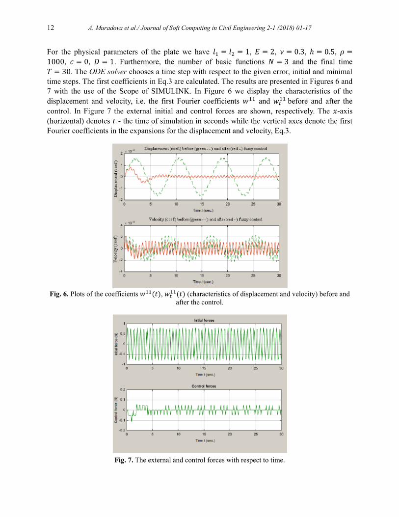
For the physical parameters of the plate we have 𝑙1 = 𝑙2 = 1, 𝐸 = 2, 𝜈 = 0.3, ℎ = 0.5, 𝜌 =
1000, 𝑐 = 0, 𝐷 = 1. Furthermore, the number of basic functions 𝑁 = 3 and the final time
𝑇 = 30. The ODE solver chooses a time step with respect to the given error, initial and minimal
time steps. The first coefficients in Eq.3 are calculated. The results are presented in Figures 6 and
7 with the use of the Scope of SIMULINK. In Figure 6 we display the characteristics of the
displacement and velocity, i.e. the first Fourier coefficients 𝑤11 and 𝑤𝑡11 before and after the
control. In Figure 7 the external initial and control forces are shown, respectively. The 𝑥-axis
(horizontal) denotes 𝑡 - the time of simulation in seconds while the vertical axes denote the first
Fourier coefficients in the expansions for the displacement and velocity, Eq.3.
Fig. 6. Plots of the coefficients 𝑤11(𝑡), 𝑤𝑡
11(𝑡) (characteristics of displacement and velocity) before and
after the control.
Fig. 7. The external and control forces with respect to time.
A. Muradova et al./ Journal of Soft Computing in Civil Engineering 2-1 (2018) 01-17 13
A detail analysis about estimates for the Fourier coefficients and the rate of convergence of the
approximate solution are given in the work [15]. The time spectral as well the time collocation
methods have a high accuracy order of computations, therefore, for small values of 𝑁 we can
obtain good results. Regarding the parameters of the exciting loading forces as many numerical
experiments have shown changes of the frequency and the amplitude of the harmonic transversal
loading in the neighborhood of them do not influence much on the control simulation. Therefore,
ones we compose the FIS for the concrete values of the frequency and amplitude we can use this
FIS in order to simulate the model for the frequency and amplitude close to the initial ones.
5. State-space representation for the linearized model
If we do not consider the nonlinear part in Eq.16 then the system Eq. 16 is a linear model which
results a spartial discretetization of the Kirchhoff-Love plate model for small deflections ([11,
21, 22]). In this case we can use both ``S-Function'' and ``State-Space'' continuous block from
the SIMULINK library.
Let us now write down the linearized model in the state space representation,
𝐯 = �̃�𝐯 + 𝐁�̃�,
𝐰 = �̃�𝐯 + 𝐃�̃�, (18)
where, 𝐯 = [𝐯1
𝐯2], �̃� = [
𝟎 𝐈−𝐌−𝟏𝐊 −𝐌−𝟏𝐂
], 𝐁 = [𝟎
𝐌−1], �̃� = [𝐈 𝟎𝟎 𝐈
], 𝐃 = [𝟎] and �̃� = 𝐏𝐪𝑁 +
𝐅𝐳𝑁. The size of the matrices �̃�, 𝐁, �̃� and 𝐃 is 2 × 𝑁2 × 2 × 𝑁2. The identity matrix I and
𝐌, 𝐊, 𝐂 have the size 𝑁2 × 𝑁2. The vectors �̃� and 𝐯 have the size 2 × 𝑁2.
We obtain analogous representations for the system Eq.17, if we neglect the nonlinear terms.
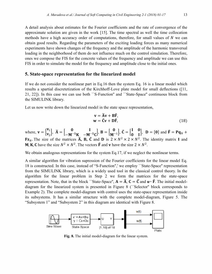
A similar algorithm for vibration supression of the Fourier coefficients for the linear model Eq.
18 is constructed. In this case, instead of “S-Function",' we employ ``State-Space'' representation
from the SIMULINK library, which is a widely used tool in the classical control theory. In the
algorithm for the linear problem in Step 2 we form the matrices for the state-space
representation. Note, that in the block ``State-Space'', 𝐀 = �̃�, 𝐂 = 𝐂 ̃and u= �̃�. The initial model-
diagram for the linearized system is presented in Figure 8 (``Selector'' block corresponds to
Example 2). The complete model-diagram with control uses the state-space representation inside
its subsystems. It has a similar structure with the complete model-diagram, Figure 5. The
“Subsystem 1” and “Subsystem 2” in this diagram are identical with Figure 8.
Fig. 8. The initial model-diagram for the linear system.

14 A. Muradova et al./ Journal of Soft Computing in Civil Engineering 2-1 (2018) 01-17
Example 2. Here we suppose that the external force 𝑄(𝑡) = sin 25𝜋𝑡 is applied at some discrete
points on the simply supported plate, exactly at the four collocation points: (𝑥1, 𝑦1) = (1/(𝑁 +
1), 1/(𝑁 + 1)), (𝑥1, 𝑦3) = (1/(𝑁 + 1),3/(𝑁 + 1)), (𝑥3, 𝑦1) = (3/(𝑁 + 1),1/(𝑁 + 1)),
(𝑥3, 𝑦3) = (3/(𝑁 + 1),3/(𝑁 + 1)). The physical parameters take the same values as in Example
1. The number of the basic functions 𝑁 = 3 and the final time is 𝑇 = 45. Here 𝑞11
= 𝑞13
=
𝑞31
= 𝑞33
= sin 25𝜋𝑡 (see Eq. 15). The initial model-diagram is given in Figure 8 and the
complete model-diagram has the same structure as in Figure 5. The amplitude in ``Sine Wave''
block is 𝐏 = (0,0,0,0,0,0,0,0,0,1,0,1,0,0,0,1,0,1)𝑇. The results are presented in Figures 9 and 10.
The suppression of the first Fourier coefficients is shown. The 𝑥-axis (horizontal) denotes 𝑡 - the
time of simulation in seconds while the vertical axes denote the first Fourier coefficients in the
expansions for the displacement and velocity, Eq.3.
Fig. 9. Plots of the coefficients 𝑤11(𝑡), 𝑤𝑡
11(𝑡) (characteristics of displacement and velocity) before and
after the control
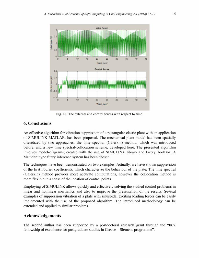
A. Muradova et al./ Journal of Soft Computing in Civil Engineering 2-1 (2018) 01-17 15
Fig. 10. The external and control forces with respect to time.
6. Conclusions
An effective algorithm for vibration suppression of a rectangular elastic plate with an application
of SIMULINK-MATLAB, has been proposed. The mechanical plate model has been spatially
discretized by two approaches: the time spectral (Galerkin) method, which was introduced
before, and a new time spectral-collocation scheme, developed here. The presented algorithm
involves model-diagrams, created with the use of SIMULINK library and Fuzzy ToolBox. A
Mamdani type fuzzy inference system has been chosen.
The techniques have been demonstrated on two examples. Actually, we have shown suppression
of the first Fourier coefficients, which characterize the behaviour of the plate. The time spectral
(Galerkin) method provides more accurate computations, however the collocation method is
more flexible in a sense of the location of control points.
Employing of SIMULINK allows quickly and effectively solving the studied control problems in
linear and nonlinear mechanics and also to improve the presentation of the results. Several
examples of suppression vibration of a plate with sinusoidal exciting loading forces can be easily
implemented with the use of the proposed algorithm. The introduced methodology can be
extended and applied to similar problems.
Acknowledgements
The second author has been supported by a postdoctoral research grant through the “IKY
fellowship of excellence for postgraduate studies in Greece – Siemens programme”.
16 A. Muradova et al./ Journal of Soft Computing in Civil Engineering 2-1 (2018) 01-17
REFERENCES
[1] Tairidis G. K., Stavroulakis G. E., Marinova D. G., & Zacharenakis E. C. Classical and
Soft Robust Active Control of Smart Beams, In: Papadrakis, M., Charmpis, D. C. Lagaros,
N. D., Tsompanakis, Y. (Eds), Computat. Struct. Dynamics and Earthquake Engineer,
CRC Press/Balkema and Taylor & Francis Group, London, UK, 2009, Ch. 11, pp. 165–
178.
[2] Tavakolpour A. R., Mailah M., Darus I. Z. M., & Tokhi O. Selflearning active vibration
vibration control of a flexible plate structure with piezoelectric actuator. Simul. Model.
Prac. and Theory 18, 2010, 516–532.
[3] Fisco N.R. & Adeli H. Smart structures: Part II: Hybrid control systems and control
control strategies. Scientia Iranica 18, 2011, 285–295.
[4] Precup R.-E., & Hellendoorn H. A survey on industrial applications of fuzzy control.
Computers in Industry 62, 2011, 213–226.
[5] Korkmaz S. A review of active structural control: challenges for engineering informatics.
Comput. and Struct. 89, 2011, 2113–2132.
[6] Preumont A. Vibration Control of Active Structures, Springer, 2002.
[7] Driankov D., Hellendoorn H., & Reinfrank M. An Introduction to Fuzzy Control, 2nd
ed., Springer-Verlag, Berlin, Heidelberg, New York, 1996.
[8] Zeinoun I. J., & Khorrami I. J. An Adaptive Control Scheme Based on Fuzzy Logic and
its Application to Smart Structures. Smart Mater. Struct. 3, 1994, 266–276.
[9] Wenzhonga Q., Jincaib S., & Yangc Q. Active control of vibration using a fuzzy control
method. J. of Sound and Vibration, 275, 2004, 917–930.
[10] Shirazi A. H. N., Owji H. R., & Rafeeyan M. Active vibration control of an FGM
rectangular plate using fuzzy logic controllers. Procedia Engineering 14, 2011, 3019–
3026.
[11] Ciarlet Ph. G. Mathematical Elasticity, v. II: Theory of Plates. Elsevier, Amsterdam, 1997.
[12] Ciarlet P., & Rabier P. Les equations de von Kármán. Springer-Verlag, Berlin,
Heidelberg, New York, 1980.
[13] Duvaut G., & Lions J. L. (1972). Les inequations en mecaniques et en physiques, Dunod.
[14] Muradova A. D. A time spectral method for solving the nonlinear dynamic equations of a
rectangular elastic plate. J. Eng. Math. 92, 2015, 83–101.
[15] Muradova A. D. & Stavroulakis G. E. Hybrid control of vibrations of smart von Kármán
plate. Acta Mechanica 226, 2015, 3463–3475.
[16] Muradova A. D., & Stavroulakis G. E. Fuzzy vibration control of a smart plate. Int. J.
Comput. Meth. in Eng. Sci. Mech. 14, 2013, 212–220.
[17] Tairidis G. Foutsitzi G., Koutsianitis P., Stavroulakis G.E. Fine tuning of a fuzzy
controller for vibration suppression of smart plates using genetic algorithms. Advances in
Engineering Software, 101, 2016, 123–135.
[18] Marinaki M., Marinakis Y., Stavroulakis G. T. Fuzzy control optimized by a Multi-
Objective Particle Swarm Optimization algorithm for vibration suppression of smart
structures. Structural and Multidisciplinary Optimization, 43, 2011, 29–42.
A. Muradova et al./ Journal of Soft Computing in Civil Engineering 2-1 (2018) 01-17 17
[19] Koutsianitis P., Tairidis G. K., Drosopoulos G. A., Foutsitzi G. A., Stavroulakis G. E.
(2017). Effectiveness of optimized fuzzy controllers on partially delaminated
piezocomposites, Acta Mechanica, 228, 1373–1392.
[20] Muradova A. D., Tairidis G. K., Stavroulakis G. T. Adaptive Neuro-Fuzzy Vibration
Control of a Smart Plate. Numerical Algebra, Control and Optimization, 7, 2017, 251–
271.
[21] Destuynder Ph., & Salaun M.. Mathematical Analysis of Thin Plate Models., Springer,
1996.
[22] Reddy J. N. Theory and Analysis of Elastic Plates and Shells, CRC Press, 2007, Taylor &
Francis.
Top Related