


Languages
Pages
Legal


FROUDE NUMBER AND SCALE EFFECTS AND FROUDE
NUMBER 0.35 WAVE ELEVATIONS AND MEAN-VELOCITY
MEASUREMENTS FOR BOW AND SHOULDER WAVE
BREAKING OF SURFACE COMBATANT DTMB 5415
by
A. Olivieri, F. Pistani, R. Wilson, L. Benedetti,
F. La Gala, E.F. Campana and F. Stern.
IIHR Report No. 441
IIHR—Hydroscience & Engineering College of Engineering The University of Iowa
Iowa City, Iowa 52242-1585 USA
December 2004

TABLE OF CONTENTS
ABSTRACT..................................................................................................................... I
ACKNOWLEDGEMENTS............................................................................................. I
LIST OF SYMBOLS ....................................................................................................... II
1. INTRODUCTION ..................................................................................................... 1
2. TEST DESIGN .......................................................................................................... 2
2.1. Facilities.............................................................................................................. 3
2.2. Model Geometries .............................................................................................. 4
2.3. Conditions........................................................................................................... 4
3. MEASUREMENT SYSTEMS, PROCEDURES, LOCATIONS AND DRE........... 5
3.1. Photo Study......................................................................................................... 5
3.2. Wave Elevations ................................................................................................. 5
3.3. Mean Velocities ................................................................................................. 6
3.4. Data Reduction Equations .................................................................................. 7
4. UNCERTAINTY ANALYSIS .................................................................................. 9
4.1. Wave Elevations ................................................................................................. 9
4.1.1. Bias Limit................................................................................................. 10
4.1.2. Precision Limit......................................................................................... 11
4.2. Mean Velocities .................................................................................................. 11
5. FROUDE NUMBER AND SCALE EFFECTS ........................................................ 11
5.1. Surface Tension and Viscous Effects ................................................................. 14
6. FROUDE NUMBER 0.35 WAVE ELEVATIONS AND MEAN VELOCITIES .... 17
7. COMPLEMENTARY CFD OBSERVATIONS ....................................................... 20
7.1. Free-Surface Wave Field and Flow ................................................................... 20
7.2. Boundary Layer and Free-Surface Vortices ....................................................... 21
8. A 3D BREAKING DETECTION CRITERION ....................................................... 22
9. CONCLUSIONS AND FUTURE WORK ................................................................ 23
REFERENCES ................................................................................................................ 25
TABLES .......................................................................................................................... 27
FIGURES......................................................................................................................... 31
i
ABSTRACT
This study is a good demonstration on how complementary EFD and CFD can
provide a powerful and advanced tool in analysing complex industrial flows. Results
are presented from a cooperative study between INSEAN and IIHR about wave and
flow field measurement about a surface combatant with focus on the 3D ship wave
breaking. At Fr=0.35, free-surface near and far fields have been measured, as well as
the velocity in some transversal planes under the bow and shoulder wave. CFD
computations have also been used to complete and extend EFD data and to
understand some particular features of the flow, such as location of vortices near the
free-surface and scars.
ACKNOWLEDGEMENTS
The research at INSEAN and IIHR was sponsored by the Office of Naval
Research under Grants NICOP: N00014-00-1-0344 and N00014-01-1-0073,
respectively, under the administration of Dr. Patrick Purtell. The research at INSEAN
was also partially sponsored by the Italian Ministry of Transportation and Navigation
in the frame of Research Plan 2000-2002.
ii
LIST OF SYMBOLS
Alphabetical Symbols
a Wave amplitude
B Bias error
Cp Pressure coefficient
e0 Voltage output related to the undisturbed water level NF
sf Sampling rate for the near field probe
FFsf Sampling rate for the far field probe
Vsf Sampling rate for velocity measurements
Fr Froude number, PPLgU /0
g Gravity acceleration
h Wave elevation
KK Calibration coefficient
LPP Length between perpendicular
Re Reynolds number, ν/0 LU
Vat Acquisition time interval for velocity measurements
NFat Acquisition time interval for the near field probe
U0 Carriage velocity
We Weber number, σρ PPLU 0
Weλ Wavelength based Weber number, σλρ0U
x Longitudinal axis
y Transversal axis
z Vertical axis NFNF yx ∆∆ , Transversal and longitudinal spacing for the grid adopted for the near
field free-surface measurements FFFF yx ∆∆ , Transversal and longitudinal spacing for the grid adopted for the far
field free-surface measurements
∆xgV , ∆zg
V Transversal and vertical spacing for the grid adopted for the velocity
measurements
iii

Greek Symbols
φα , Measured pitch and yaw angles of a velocity vector in 5-hole Pitot
probe coordinates
pp φα , 5-hole Pitot probe preset pitch and yaw angles
λ Wave length
ρ Water density
σ Surface tension
θ Sensitivity coefficient in uncertainty assessment; and local wave
steepness
ν Kinematic viscosity
iv
FROUDE NUMBER AND SCALE EFFECTS AND FROUDE
NUMBER 0.35 WAVE ELEVATIONS AND MEAN-VELOCITY
MEASUREMENTS FOR BOW AND SHOULDER WAVE
BREAKING OF SURFACE COMBATANT DTMB 5415
1 INTRODUCTION
The motion of marine vehicles traveling at sea usually leads to the formation of
steep diverging bow and stern waves, possibly breaking. Depending on speed and
geometry, a sequel of interesting phenomena follows: the generation of vorticity in the
breaking region, the appearance of free-surface scars, and the entrainment of air, to
name a few.
The present report is aimed at illustrating an experimental campaign focused in
providing detailed experimental data for the 3D wave breaking generated by a fast
displacement ship model, the DTMB 5415, conceived by David Taylor Model Basin as
a preliminary design for a surface combatant (ca. 1980) with a sonar dome bow and
transom stern.
The experimental campaign was carried out in the framework of a long term
international collaboration between INSEAN and IIHR (see also [1], [17]) focused in
providing detailed experimental data for a fast displacement ship model.
The purpose of present investigation is to increase our knowledge of the flow
field near an advancing surface ship when breaking waves are produced. This work
also stems from the difficulty in modeling this complex flow and hence from the
strong need of accurate and tailored experimental campaigns dedicated to collecting
data for benchmarking.
As Duncan [6] points out, recent literature dedicated to the subject is
concentrated to PIV measurements of the breakers in the bow waves of a ship model,
e.g. Dong et al. [9] and Roth et al., [10]. In both these studies the focus is on the flow
within the attached liquid sheet close to the stem of the ship model, to analyse the
structure of the bow wave, and do not extend the investigation to the downstream
evolution of the free-surface flow after the breaking, including wave induced vortices.
Analyzing the flow past a ship in drift condition, Longo and Stern [20] show
the presence of a bow wave breaking induced vortex on the suction side of the model.
1
However, previous data collected for zero drift condition does not show bow wave
breaking.
Here, a much more complete set of data is presented, providing for the first
time a complete and accurate description of bow wave breaking at least for quasi-
steady condition. After a detailed photo study of the free-surface pattern is presented,
local flow measurements, including near field wave elevation, far field wave elevation
and velocity measurements under the breaking waves are reported and analyzed.
The report is organized as follows: the test design is reported in chapter 2,
describing the test conditions, the model geometry and the facility. Next, in chapter 3
the measurement system is reported, together with procedures and data reduction
equations. Chapter 4 reports the procedures for the uncertainty analysis. Scale and
Froude number effects are illustrated in chapter 5, whereas wave elevations and mean
velocities measurements at Froude number 0.35 are reported and analysed in chapter 6.
Complementary CFD observations are made in chapter 7 and a criterion for wave
breaking detection is proposed in chapter 8. Finally, conclusions and future plans are
given in chapter 9.
2. TEST DESIGN
The present experimental campaign is focused in providing detailed EFD data
appropriate for physics understanding, model development and CFD validation for 3D
wave breaking generated by a fast displacement ship model (surface combatant 5415).
The tests were conducted in the INSEAN basin n. 2 (fig. 1) with the 2340
INSEAN model that is 5.72 m long (λ = 24.824). Breaking wave pattern photo study
for Froude number varying from Fr = 0.28 (design speed) and Fr = 0.45, including
Fr = 0.41 (flank speed) was carried out in order to select the best Froude number for
local flow measurements.
The Froude number Fr = 0.35 was selected in order to have a large region of
wave breaking, but also a relatively steady wave pattern.
In parallel the same photo-study was conducted on the geosym 3.048 m long
5512 (λ = 46.6), at the IIHR towing tank (fig. 2) for comparison and evaluation of the
scale effect, since 5512 has been used for the collection of a considerable amount of
EFD data for CFD results validation, especially for unsteady flow. Full-scale photos
were also used in comparison and for the evaluation of the scale effect.
2

Local flow measurements, including near field wave elevation, far field wave
elevation and velocity measurements under the breaking waves were accomplished.
Near field wave elevation measurements were carried out from the bow to
about midship using the servo-mechanic (finger) probe Kenek SH by single point
measurements, which allow evaluating the mean and the rms value of the wave height.
Far field wave elevation was reconstructed by longitudinal cuts that were
measured by means of an array of capacitance wire wave gauges mounted on a sliding
guide as described in [1]. For these measurements, only the mean wave height was
evaluated.
Three component velocity measurements were carried out by 5-hole Pitot probe
in correspondence of both bow and shoulder breaking waves. The mean velocity was
evaluated on four cross planes along the port side of the model.
Uncertainty assessment for wave elevation and velocity measurements were
evaluated following the AIAA Standard S-071 1995.
In the following, the Cartesian frame of reference is considered fixed to the
hull, with the origin at the intersection of the fore perpendicular with the undisturbed
water plane. In particular, x, y and z axes are in the direction of the uniform flow,
starboard side of the hull and upward, respectively. All lengths are normalized by the
model length between perpendiculars LPP = 5.72 m (INSEAN 2340 model).
2.1. Facilities
The smaller model (IIHR 5512) was tested in the IIHR towing tank (100 m
long, 3.048 m wide and 3.048 m deep). The IIHR tank is equipped with an electric-
motor operated drive carriage, cable driven by a 15-horsepower motor and capable of
speeds of 3 m/s. Sidewall and endwall beaches enable twelve-minute intervals between
carriage runs. The towing-tank water is supplied by the city of Iowa City.
The larger model (INSEAN 2340) was tested in the INSEAN basin N. 2 (220 m
long, 9 m wide and 3.6 m deep). INSEAN basin N. 2 is equipped with a single drive
carriage that is capable of speeds of 10 m/s. Sidewall and endwall beaches enable 20-
minute intervals between carriage runs. The towing tank water is spring water.
Both the IIHR and INSEAN towing tanks use fresh water in which salinity is
less than 0.5 ppt, while for the sea it is about 30 ppt. This difference mainly influences
the air entrainment in the breaking waves.
3
All data related to the facilities and test conditions are reported in table 1.
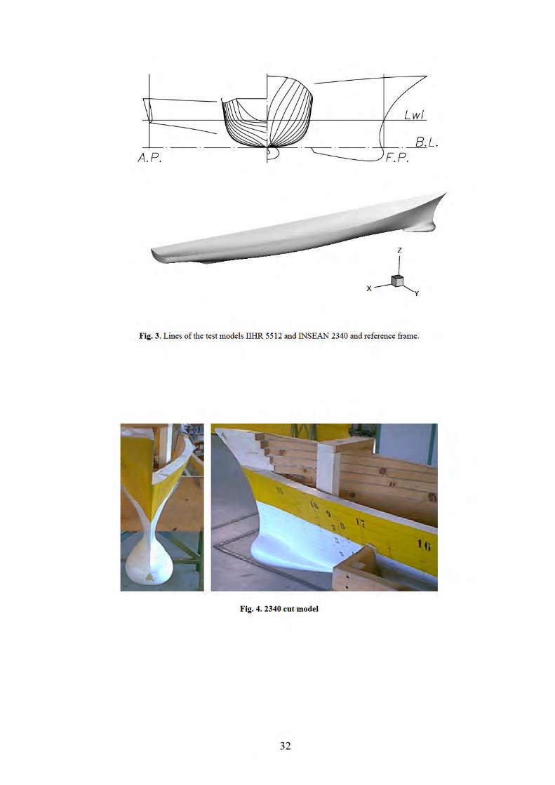
2.2. Model Geometries
The IIHR 5512 and the INSEAN 2340 models are geosyms of the DTMB 5415
model, originally conceived as a preliminary design for a surface combatant ship. The
2340 is identical to the 5415, while 5512 is differently scaled and its length between
perpendiculars is LPP = 3.048 m. The models present a transom stern and a bulbous
bow of particular shape, designed for sonar lodging. In fig. 3 the lines of the 2340
model are shown. The main geometric parameters of the two test models are given in
table 2. All tests were performed in bare hull condition.
IIHR 5512 was constructed in 1996 at the DTMB model workshop from
molded fiber-reinforced Plexiglas. Turbulence stimulation is at x = 0.05 with
cylindrical studs having 3.2 mm diameter, 1.6 mm height, and 10.0 mm spacing.
INSEAN 2340 was constructed in 1998 at the INSEAN model workshop from
a blank of laminated wood and a CNC machine. Turbulence stimulation is at x = 0.05
with cylindrical studs having 3.0 mm diameter, 3.0 mm height, and spaced 30.0 mm.
The geometry offset measurement system consists of computer-aided design (CAD),
hand-cut templates, level table, right angle, plumb, and rulers and feeler gauges. The
data is reduced by computing crossplane and global average values for the error in the
offsets for each coordinate and for S.
2.3. Conditions
Reproducing ship breaking waves in the towing tank needs accurate control
over many parameters and test conditions, leading to a high repeatability of the flow.
Nevertheless, the inherent disadvantage of laboratory experiments is the effect of
surface tension on the breaking. Indeed, depending on the size and on the speed of the
model, surface tension effects can prevent the wave to overturn and may significantly
reduce the air entrainment. At all events, photographic studies were done at INSEAN
and IIHR on both the 5512 and 2340 models with the aim of documenting the scale
effect on the wave breaking and choosing for 2340 the best test conditions for the
wave elevation and velocity measurements.
As a result of the visualizations quite steady, well-developed breaking
conditions were found in the Froude number range 0.3 – 0.4. At Fr = 0.3 the flow
4

pattern was almost completely steady, but the breaking extent was not very large and
its intensity was not very high. On the opposite, at Fr = 0.41, the wave breaking extent
and intensity were respectively larger and higher, whereas the flow pattern was
observed to be less steady. Eventually, Froude number 0.35 was selected for the
experimental campaigns as a trade-off among the opposite needs.
During the tests, the model was held fixed, with trim and sinkage (tab. 3) set to
the values previously determined in unrestrained conditions [1]. The experimental
conditions correspond to Froude number Fr = 0.35, Weber number We = 734 and
Reynolds number Re = l.5×107 based on free stream velocity U0 = 2.621 m/s, local
gravity acceleration g = 9.8033 m/s2, water density ρ = 998.5 kg/m3, kinematic
viscosity ν = 1.09x10⁻⁶ m2/s, surface tension σ = 0.0734 N/m and salinity < 0.5 ppt.
3. MEASUREMENT SYSTEMS, PROCEDURES, LOCATIONS AND DRE
3.1. Photo Study
The photo study was made both at IIHR (with the 5512 model) and at INSEAN
(with the 2340 model). Photos of the free surface around the bow were taken in order
to observe the topology of the bow breaking wave and evaluate the scale effect on the
breaking itself. The photos were made for a wide range of Froude numbers, but here
only those taken at moderate and high Froude numbers are shown, for which the wave
breaking is clearly observable for both model scales (Fr = 0.28, 0.3, 0.325, 0.35, 0.375,
0.41 and 0.45). For Fr = 0.28 and Fr = 0.35, photos of the full scale (DDG 51) are also
shown for comparison.
3.2. Wave Elevations
The wave height was measured by a servo-mechanic probe (Kenek SH),
mounted on a system of guides fixed to the carriage. The wave field was obtained by
point wise measurements from the bow down to about midship.
In order to get wave elevation measurements as close as possible to the hull,
some part of the port side of the model was cut off as shown in fig. 4.
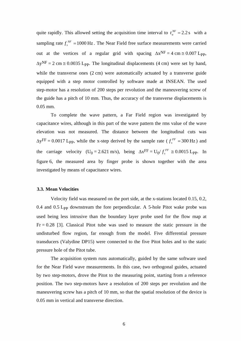
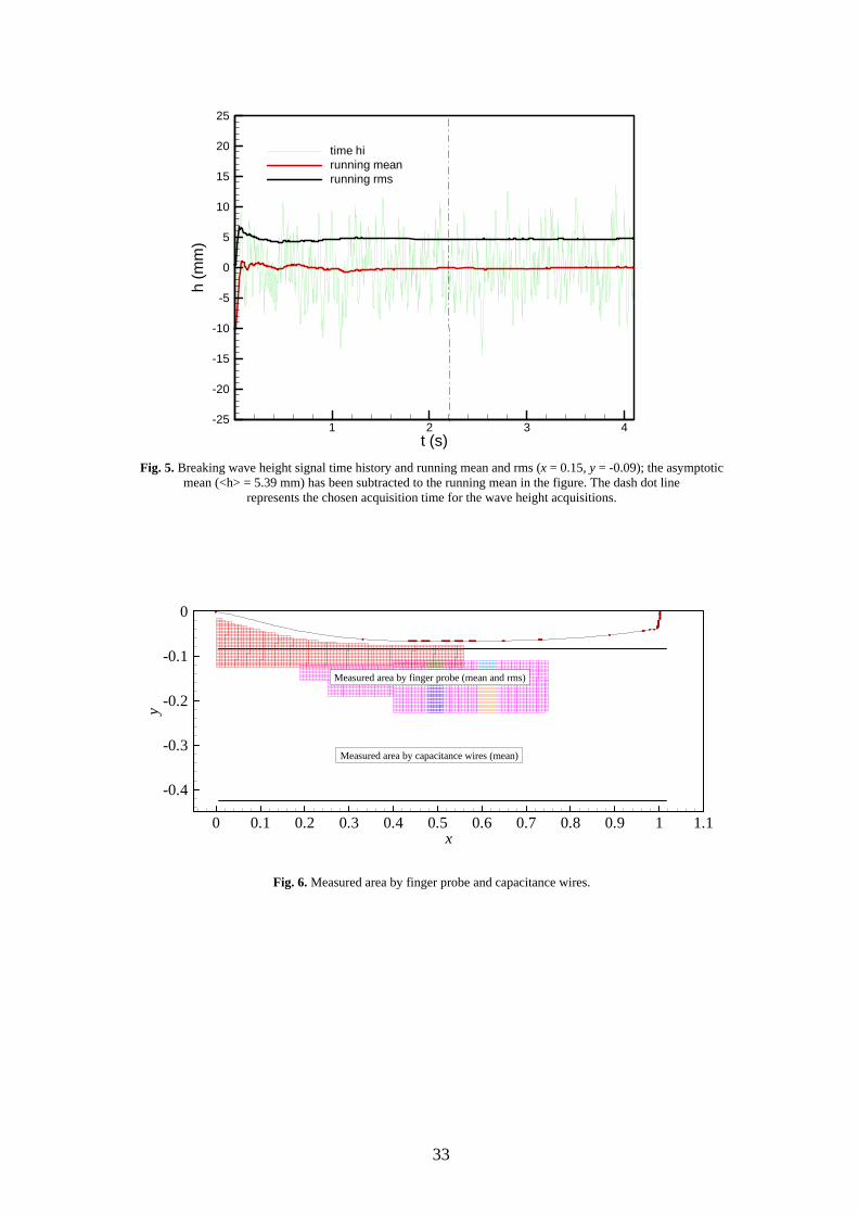
The carriage acceleration was lowered as much as possible in order to reduce
the wave fluctuations due to the transient wave components. Time history and running
mean and rms value for a measuring point inside the breaking region (x = 0.15,
y = -0.09) are shown in figure 5. Both mean and rms converged to an asymptotic value
5
quite rapidly. This allowed setting the acquisition time interval to with a
sampling rate . The Near Field free surface measurements were carried
out at the vertices of a regular grid with spacing ∆xNF = 4 cm ≅ 0.007 LPP,
∆yNF = 2 cm ≅ 0.0035 LPP. The longitudinal displacements (4 cm) were set by hand,
while the transverse ones (2 cm) were automatically actuated by a transverse guide
equipped with a step motor controlled by software made at INSEAN. The used
step-motor has a resolution of 200 steps per revolution and the maneuvering screw of
the guide has a pitch of 10 mm. Thus, the accuracy of the transverse displacements is
0.05 mm.
s 2.2 =NFat
Hz 1000 =NFsf
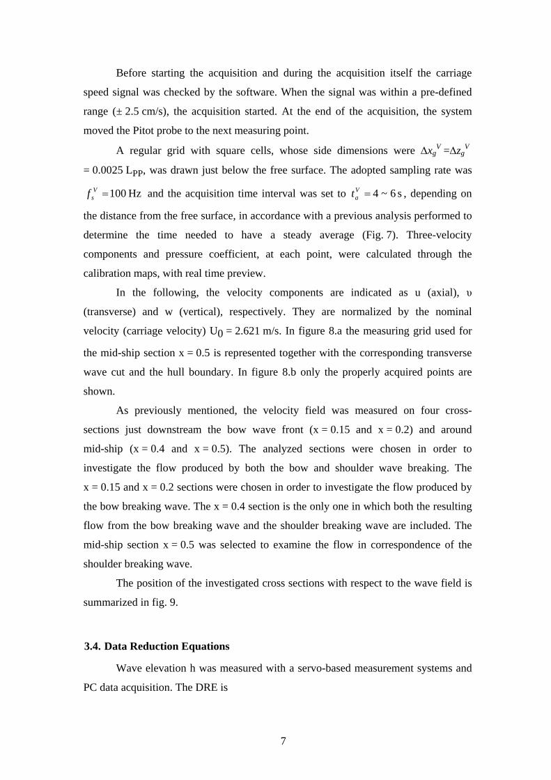
To complete the wave pattern, a Far Field region was investigated by
capacitance wires, although in this part of the wave pattern the rms value of the wave
elevation was not measured. The distance between the longitudinal cuts was
∆yFF = 0.0017 LPP, while the x-step derived by the sample rate ( ) and
the carriage velocity (U0 = 2.621 m/s), being ∆xFF = U0/ ≅ 0.0015 LPP. In
figure 6, the measured area by finger probe is shown together with the area
investigated by means of capacitance wires.
Hz 300 =FFsf
FFsf
3.3. Mean Velocities
Velocity field was measured on the port side, at the x-stations located 0.15, 0.2,
0.4 and 0.5 LPP downstream the fore perpendicular. A 5-hole Pitot wake probe was
used being less intrusive than the boundary layer probe used for the flow map at
Fr = 0.28 [3]. Classical Pitot tube was used to measure the static pressure in the
undisturbed flow region, far enough from the model. Five differential pressure
transducers (Valydine DP15) were connected to the five Pitot holes and to the static
pressure hole of the Pitot tube.
The acquisition system runs automatically, guided by the same software used
for the Near Field wave measurements. In this case, two orthogonal guides, actuated
by two step-motors, drove the Pitot to the measuring point, starting from a reference
position. The two step-motors have a resolution of 200 steps per revolution and the
maneuvering screw has a pitch of 10 mm, so that the spatial resolution of the device is
0.05 mm in vertical and transverse direction.
6
Before starting the acquisition and during the acquisition itself the carriage
speed signal was checked by the software. When the signal was within a pre-defined
range (± 2.5 cm/s), the acquisition started. At the end of the acquisition, the system
moved the Pitot probe to the next measuring point.
A regular grid with square cells, whose side dimensions were ∆xgV =∆zg
V
= 0.0025 LPP, was drawn just below the free surface. The adopted sampling rate was
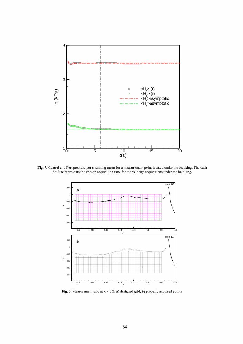
and the acquisition time interval was set to , depending on
the distance from the free surface, in accordance with a previous analysis performed to
determine the time needed to have a steady average (Fig. 7). Three-velocity
components and pressure coefficient, at each point, were calculated through the
calibration maps, with real time preview.
Hz 100 =Vsf s 6~4 =V
at
In the following, the velocity components are indicated as u (axial), υ
(transverse) and w (vertical), respectively. They are normalized by the nominal
velocity (carriage velocity) U0 = 2.621 m/s. In figure 8.a the measuring grid used for
the mid-ship section x = 0.5 is represented together with the corresponding transverse
wave cut and the hull boundary. In figure 8.b only the properly acquired points are
shown.
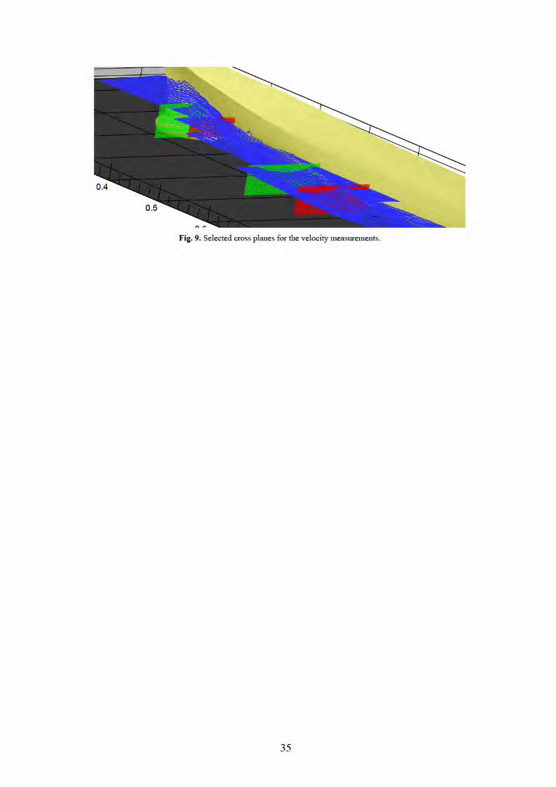
As previously mentioned, the velocity field was measured on four cross-
sections just downstream the bow wave front (x = 0.15 and x = 0.2) and around
mid-ship (x = 0.4 and x = 0.5). The analyzed sections were chosen in order to
investigate the flow produced by both the bow and shoulder wave breaking. The
x = 0.15 and x = 0.2 sections were chosen in order to investigate the flow produced by
the bow breaking wave. The x = 0.4 section is the only one in which both the resulting
flow from the bow breaking wave and the shoulder breaking wave are included. The
mid-ship section x = 0.5 was selected to examine the flow in correspondence of the
shoulder breaking wave.
The position of the investigated cross sections with respect to the wave field is
summarized in fig. 9.
3.4. Data Reduction Equations
Wave elevation h was measured with a servo-based measurement systems and
PC data acquisition. The DRE is
7
( )PP
0
LeeK
h K −=
, (1)
where e is the voltage output acquired by the PC and KK is the calibration coefficient.
e0 is the voltage output related to the undisturbed free surface; it is acquired before
every carriage run.
The measurement system consisted of a Kenek SH servo- mechanic probe,
signal conditioner, 2D traversing system, 12-bit AD card and carriage PC. The servo
probe, signal conditioner, and carriage PC AD card were statically calibrated on the
traverse system to determine the voltage-wave elevation relationship.
Velocity fields data (u, υ, w, Cp; x = 0.15, x = 0.2, x = 0.4, x = 0.5) were
measured by 5-hole Pitot probe/differential pressure transducer based measurement
system and PC data acquisition. The DREs are
( +φ+φα= ppp sinVYcoscosVXzyxu ),,( ) cpp UcossinVZ φα (2)
( −φ+φα−= ppp cosVYsincosVXzyxυ ),,( ) cpp UsinsinVZ φα (3)
( ) cpp UsinVXcosVZzyxw α−α=),,( (4)
2
2
2
22
c
c
c
op ρU
VPρHρU
ppzyxC
′−′=
−=
)(),,(
(5)
where, αφ coscosVVX ′= (6)
φsinVVY ′= (7) αφ sincosVVZ ′= (8)
MρMV
′=′ 2
(9)
spbtc HHHHH4M ′−′−′−′−′=′ (10)
)HHHHH4(HHK
spbtc
bt′−′−′−′−′
′−′=′
(11)
)HHHHH4(HH
Lspbtc
ps′−′−′−′−′
′−′=′
(12)
( pp φα , ) are the 5-hole Pitot probe preset pitch and yaw angles, respectively,
( φα , ) are the measured pitch and yaw angles of the velocity vector in 5-hole Pitot
8
probe coordinates, respectively, and jH ′ , (j = c, t, b, p, s) are the measured pressures
for the center, top, bottom, port, and starboard holes, respectively. The side holes of
the static Pitot probe measured the reference pressure (p0).
The primed variables designate the local measured values and coefficients
computed using local measured values, whereas, unprimed variables (K, L, M, P)
designate variables from a wind tunnel calibration of the 5-hole Pitot probe [1]. ( φα , )
are obtained from ( ) and their corresponding 5-hole Pitot probe calibration
coefficients (K, L). (
L ′′,K
φα , ) are then used to obtain (M, P) from their corresponding
5-hole Pitot probe calibration coefficients.
4. UNCERTAINTY ASSESSMENT
Uncertainty assessment of the results was carried out following the AIAA
Standards S-071-1995 [4] for both wave elevation and velocity.
The bias limit was evaluated by taking into account the more important sources
of error. The precision limit was evaluated by 10 repeated tests for both wave elevation
and velocity measurements.
4.1. Wave Elevations
Wave elevation was measured in the near field using a Kenek SH
servo-mechanic probe, which DRE is
( )PP
0
LeeK
h K −=
(1)
The bias limit was evaluated based on the propagation of the elemental biases
into the wave elevation bias, while the precision limit was evaluated on 10 repeated
tests directly on the wave elevation data.
The wave elevation depends on a series of variables including the measuring
point and the carriage velocity U0:
),,,,,,( 0 OPPK UyxLeeKfh = (13)
The sensitivity coefficients are:
ppKK L
eeKh
K
0−=
∂∂
=θ (14)
9
pp
Ke L
Keh
=∂∂
=θ (15)
pp
Ke L
Keh
−=∂∂
=0
0θ
(16)
20 )(1
pp
K
ppppL L
eeKh
LLh
PP
−−=⋅−=
∂∂
=θ (17)
The sensitivity coefficients related to the measuring point coordinates are
obtained deriving the acquired data using finite differences;
xh
x ∂∂
=θ (18)
yh
y ∂∂
=θ (19)
The last term,
00 U
hU ∂
∂=θ
(20)
should be determined by performing the test at different velocities for the measured
field. Nonetheless being the velocity bias very small (≅ 3 mm/s [5]), this term was
neglected in the estimation of the bias limit. The precision limit was determined
directly on h.
4.1.1 Bias Limit The bias on e and e0 was obtained by the ratio between the
voltage range of the acquisition board (± 10V) and its resolution (212). This value was
normalized with the used range by the sensor that was ∆e = ± 3V. Being this bias
present both on e and on e0, the total bias due to the A/D conversion is obtained by:
eD/A BB 2= (21)
The bias on KK is given by the manufacturer of the sensor as 0.2% and it was
checked before and after the tests (BK in tab. 4).
The bias on the model length is BLPP = 1mm [1] and it was considered
negligible with respect to the other elemental biases.
The biases on x and y, which individuate the measuring point, were determined
considering the sequence of the needed measurements in order to set the position of the
sensor in the model reference frame (Bx = 0.707 mm, By = 0.866 mm).
10
The evaluation of the sensor position with respect to the model, involves many
difficult measurements, including the use of tools such as squares and plumb line. For
this reason, we decided to dismount the model and the sensor every time we performed
a carriage run for the precision limit evaluation. In this way, the errors on the
measuring point were transformed in random-type errors and they were automatically
included in the h precision limit.
4.1.2 Precision Limit The precision limit was determined in three different
points located in the non-breaking, close to the breaking and breaking region
respectively. The locations of the three points are reported in table 4 together with the
values of the considered biases BA/D and BKK, the precision limits and the total
uncertainties for the mean and for the rms value of the wave elevation.
4.2. Mean Velocities
The bias limit on the velocity was determined following the procedure
elaborated in [1]. Elemental errors associated to the 5 pressure values given by the
Pitot, the Pitot position with respect to the model, the preset angles, the flow angles,
the carriage velocity, P and M coefficients [1] and velocity gradient [3] were
considered to estimate the bias limit. Its value is comparable with the ones obtained in
a previous study on the boundary layer flow of the same model at Fr = 0.28 [1]. The
precision limit was determined directly on the three velocity components for a
measuring point at section x = 0.20, just under the breaking (y = - 0.1015, z = - 0.005).
The precision values are also comparable with the ones of the Fr = 0.28 boundary layer
data. Here the percentage values are lower just because of the larger range of variation
of the transverse and vertical velocity components.
Bias limit, precision limit and total uncertainty for the point located at
x = 0.20, y = - 0.1015, z = - 0.005, are given in table 5.
5. FROUDE NUMBER AND SCALE EFFECTS
For the purposes of this paper, the photo study of the wave breaking generated
by the two scaled models and performed at moderate and high Froude numbers
(Fr = 0.28, 0.3, 0.325, 0.35, 0.375, 0.41 and 0.45) using same perspective views was
compared with full scale pictures at Fr = 0.28 and Fr = 0.35. Throughout the series of
11

pictures the influence of the physical quantities and the main nondimensional
parameters on the wave breaking are studied.
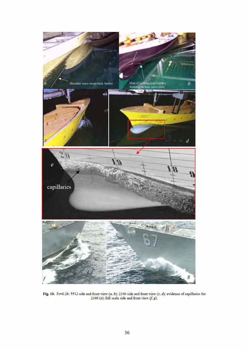
The lowest analyzed speed is Fr = 0.28. 5512 (figs. 10.a, 10.b) shows small
regions of bow wave curling and spilling-type breaking with capillary waves along toe
and shoulder wave with roughened crest region with capillary waves hinting at
spilling-type breaking wave. Model 2340 (figs. 10.c, 10.d) shows more curling and
developed spilling-type bow wave breaking. The role of the surface tension is shown
by the enlarged view in fig. 10.e. Moving downstream with the flow, the breaking
grows in amplitude and ripples become visible just upstream the wave “toe” [2]. The
shoulder wave breaking (not visible in fig. 10.c and 10.d) resembles a 2D spilling
wave breaking as per model 5512 but with higher intensity.
For Fr = 0.28, photos of the full scale are shown for comparison. Figure 10.g
shows that differently from both models, the real ship bow wave is a spilling type
breaking with generation of spray, splash and droplets, which lead to a significant
production of white water. The shoulder wave is also a spilling breaker type with
generation of whitewater along crest.
For Fr = 0.3 and Fr = 0.325, both 5512 and 2340 results are similar to those of
Fr = 0.28 but with increased regions and curling of bow wave close to hull especially
for 2340 and two small scar lines along back of bow wave for 2340.
In particular, at Fr = 0.3, model 5512 shows (fig. 11.b) a slightly intense bow
wave breaking, still affected by the action of the surface tension. The shoulder wave
breaking (fig. 11.a, 11.b) is quite similar to the one observed at Fr = 0.28, with the
crest swept back more than in the previous case. Small scars begin to form just behind
the bow breaking (fig. 11.a). Model 2340 shows a more intense bow wave breaking
with respect to Fr = 0.28 and streamlined scars begin to appear on the free surface
(fig. 11.c). These will become more visible at higher Froude numbers.
At Fr = 0.325 (fig. 12) the breaking scenario is quite similar to the one
observed at Fr = 0.3 for both models, although a number of details begin now to
emerge. By comparing fig. 11.a and 12.a, it can be seen that the bow breaking is now
more intense and the wake left behind by the breaker extends further normally to the
wave front, i.e. toward the hull for the 5512. Likewise, in fig 12.a, small scale surface
disturbances left by the breaking appear on the left of the bow wave, covering a wider
area behind the breaking front. For the 2340, scars are also more pronounced although
they disappear rapidly downstream (fig. 12.c).
12

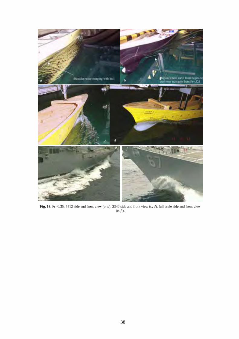
At Fr = 0.35 (fig. 13) more details are clearly identifiable and the whole picture
is compared to full scale visualization. Model 5512 exhibits (fig. 13.b) a bow breaking
wave. Moving along the crest of the bow wave, the wave front begins to rise at the
extreme bow and a bulge grows onto the top of the bow wave. The air entrainment is
strongly limited by the action of the surface tension.
Figures 13.c and 13.d show the downstream and upstream perspective of the
bow breaking wave for the 2340 model. 2340 shows large regions of bow wave almost
steady plunging breaking close to hull and spilling breaking further from hull. Also
visible are two large scars downstream of the bow wave and a large region shoulder
wave spilling breaker. Full scale shows spilling breaking bow wave with white water
along crest and back merging with shoulder wave both with splash, initially plunging
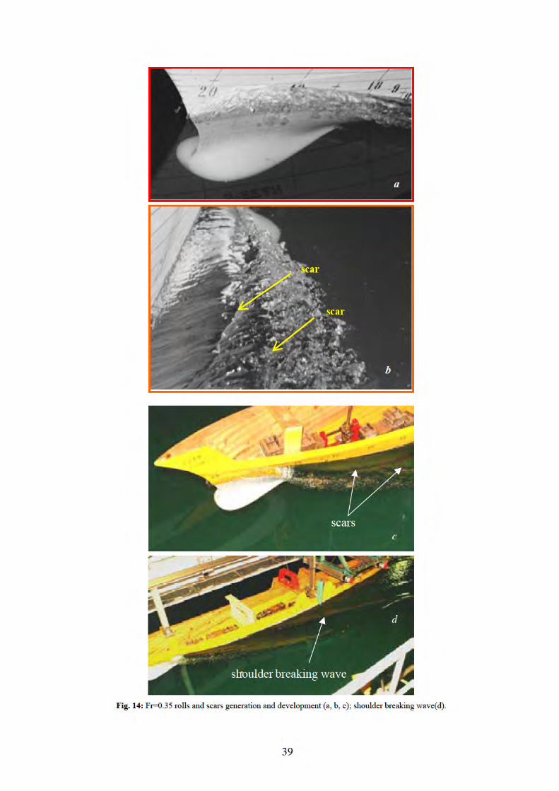
and then becoming spilling. Fig. 14.a shows the rise of the free surface at the extreme
bow and overturn of the wave crest. Fig. 14b shows scars on back of breaking bow
wave. These scars extend downstream to about midship (figs. 14.c and 14.d). The
shoulder wave exhibits a low energetic content developing a “2D spilling”-like wave
breaking as shown in figure 14.d. The wave breaking scenario observed for the 2340
qualitatively resembles the full scale scenario except for the amount of generated white
water (figs. 13.e and 13.f).
For Fr = 0.375, 0.41 and 0.45, both 5512 and 2340 photos show similar
incremental trends as per Fr=.35, including large effects unsteady flow (e.g. ejections,
etc.).
At Fr = 0.375 the 5512 shows (fig. 15.a and 15.b) a quite developed spilling
bow breaker. The shoulder wave is merging with the hull. The near field generated by
the 2340 is quite similar to the previous case (Fr = 0.35), except for the presence of
stronger water ejections.
At Fr = 0.41 (fig. 16) the bow wave breaking of the 5512 appears in form of
plunging breaker. Air entrainment is considerably increased in this case, but looking to
the starboard side, differences between 15.a and 15.c show that the role of the surface
tension for the smaller model is still relevant. For the 2340, overturns are quite evident
and the plunging nature of the breaker is clearly visible in figure 16.c.
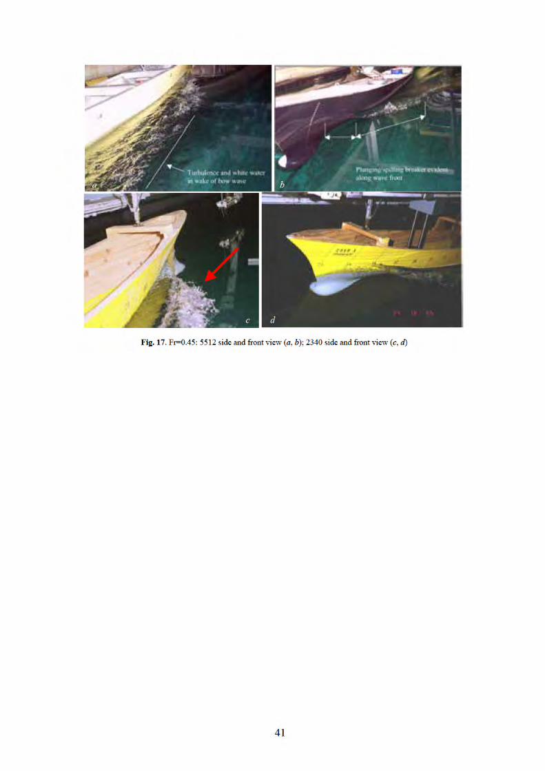
At Fr = 0.45 (fig. 17) the bow wave breaking of the 5512 is characterized by
the presence of both plunging-type breaker (upstream) and spilling-type breaker
(downstream) as shown in figure 17.b. The bow wave breaking of the 2340 is entirely
13
plunging-type and generates a system of streamlined rolls that evolve along the hull
(Fig. 17.c).
As a summary of the photo study we can state that scale effects in wave
breaking are significant when comparing 5512 scenario vs. 2340, with increasing
differences for increasing Fr. Scale effects are still observable for 2340 vs. full scale
although some particular features of the full scale flow are reproduced by the 2340
model wave breaking. Fr = 0.35 is the first speed with a quite steady, well developed
breaking with a sufficiently high energetic content. For Froude numbers higher than
Fr = 0.375 unsteadiness appears and the bow breaking wave generates strong water
ejections that made the measurements troublesome. Consequently, Fr = 0.35 was
finally selected for the near wave field and the velocity measurements for the 2340
model.
5.1. Surface Tension and Viscous Effects
In the following, based on the photo study and literature results about waves
and wave breaking, the physical quantities that influence the wave breaking
development in model scaled experiments are analyzed.
As known from literature, small scale wave breaking is strongly influenced by
surface tension [2,16]. Furthermore, the wave breaking is intimately connected with
turbulence generation that is a viscous phenomenon. Hence, the parameters to be
considered other than Froude number (Fr), are at least, Weber number (We) and
Reynolds number (Re), whose definitions are:
LgUFr =
(22);
σρ LUWe =
(23);
νLURe =
(24).
being U and L the model speed and length, g the gravity acceleration, ρ and ν the
fluid density and kinematic viscosity and σ the water-air interface surface tension. In
table 6 the Froude, Weber and Reynolds numbers for 5512, 2340 and full scale are
given for all the analyzed conditions, while the corresponding physical quantities are
listed in table 7.
14
In order to satisfy the Froude similarity, the scaled model experiments are
performed at a lower velocity with respect to the full scale and this automatically
implies the violation of the Weber and Reynolds similarity. It is then fundamental to
assess experimental conditions in which surface tension and viscous effects do not
change too much the wave breaking characteristics at model scale, with respect to the
applications (full scale). To this aim, important indications may be gathered from the
photo study described before.
Because the surface tension term depend on the magnitude of the radius of
curvature of the free surface, the role played by surface tension may be quite different
for breaking and non breaking (regular) waves, and in the latter case it is also of
relevance the wavelength. In a previous work [17], Stern et al. focused on comparing
resistance, sinkage and trim, and wave pattern measurements on the same model
geometry (the DTMB 5415) between three institutes (two of the institutes used 5.72 m
models whereas the third used a smaller 3.048 m model). Scale effects for the smaller
model were only evident for resistance and trim tests for Fr > 0.26 and Fr > 0.33,
respectively, while in the low Froude number range, corresponding to a non-breaking
wave pattern, scale effects were found to be almost negligible. In the present
campaign, the photo study revealed that the smaller scale experiment does not generate
a developed breaking for Froude number lower than Fr = 0.41 (We = 456, see table 6),
while the larger scale experiment exhibits a well developed breaking starting from
Fr = 0.3 (We = 627).
A further analysis has been carried out the considering the wavelengths of the
diverging wave systems as reference lengths in the Weber number (Weλ). The values
of these wavelengths are reported in table 8 together with the corresponding Weber
numbers (Weλ)1. As observed in the photo study, for the smaller model (5512), the
surface tension is less dominant in the wave breaking for Fr > 0.41, while for the larger
one (2340), its effect is present up to Fr = 0.3. It is noticeable that the limiting
condition corresponds for both cases to wavelengths of the diverging waves of 41 cm
and velocity of 2.24 m/s. The related Weber number Weλ is in both cases Weλ =168.
It is interesting to notice that, although the minimum wavelength needed in
order to have pure gravity waves is about 1 m [16], is commonly accepted that for
1 In table 8 the λDW value of the 2340 model at Fr = 0.35 is obtained from the experimental data, and serves as a base for calculating all the other values for different Froude numbers and model lengths.
15
wavelength larger than 40 cm the effect of the surface tension can be neglected2, in
agreement with present findings.
Furthermore, the influence of the viscosity should be considered.
The Reynolds number for the full scale is about two orders of magnitude larger
than the model Reynolds number. Furthermore, being the first stage of the breaking
generated at the bow, a local Reynolds number (e.g. based on the axial abscissa x) has
to be considered in order to relate the wave breaking with viscous phenomena, with
particular attention to the laminar/turbulent transition. Considering the critical
Reynolds number for the flat plate (Rec ≅ 3.5×10⁵), the smaller model flow undergoes
the laminar/turbulent transition at about x = 0.05 at the maximum speed (Fr = 0.45)
and x = 0.08 at Fr = 0.28, whereas the flow around the larger model undergoes the
turbulent transition at x = 0.02 at Fr = 0.45 and x = 0.03 at Fr = 0.28. The full scale
flow is turbulent for x > 0.005.
On the other hand, it has to be noticed both models are provided by turbulence
stimulators placed at x = 0.05.
Nonetheless, figures 10.a and 10.b show that wave breaking at Fr = 0.28 for the
5512 starts to develop downstream with respect to the 2340 and this could be related to
the low Re nature of the flow around the 5512 upstream x = 0.08.
Furthermore, figures 10-17 show that the bow wave breaking of the 2340
generates free surface turbulence for all the analyzed cases, while 5512 generates free
surface turbulent flow only for Fr ≥ 0.41. Moreover, the scars generated by 2340 at
Fr = 0.35 are clearly turbulent (fig. 14), whereas the scars generated by 5512 appear to
be laminar (figs. 11.a - 17.a).
A better indication on the importance of the viscous dissipation in the wave
breaking development should be given by the (local) turbulent Reynolds number,
based on the intensity of the velocity fluctuations and Taylor micro-scale [8].
However, the estimate of this parameter requires the use of a different system for the
velocity measurement, as PIV, LDV or hot-film anemometer and it cannot be obtained
with present data.
2 Experimental results obtained by Duncan for 2D waves produced by a submerged hydrofoil gave a wavelength of about 41 cm [7] and have been often taken as a reference benchmark in the development and validation of numerical codes not taking into account surface tension forces.
16
Another aspect that should be analyzed is the difference in salinity between the
seawater and the water used for the experiments. In fact, salinity changes the density
and consequently Reynolds and Weber number, although, differences caused by
density changes in the value of these two parameters are very small. In addition, the
surface tension increases with salinity, although the role of the surface tension in the
full scale breaking can be neglected, due to the large value of the waves curvature
radius.
The more important effect of salinity relates with air entrainment and
production of white water. In fact, the percentage of the dissolved gases decreases
when salinity increases [13], so that bubble generation and air entrainment could be
rather different in the laboratory wave breaking with respect to seawater wave
breaking.
Nevertheless, the influence of the salinity on free surface topology and flow
evolution can be considered a minor source of discrepancies between the model and
the full scale breaking with respect to scale effects [18].
6. FROUDE NUMBER 0.35 WAVE ELEVATIONS AND MEAN
VELOCITIES
On the basis of the previous considerations the 2340 model was selected for the
wave breaking analysis focusing the measurements on the flow field at Fr = 0.35.
The reconstruction of the wave elevation field was done in terms of the mean
value (near and far fields) and rms value (near field), whose patterns are shown in
figures 18.a and 18.b. In figure 18.a, capacitance wires data are shown together with
the finger probe data for the mean wave elevation. The highest value of the wave
elevation in the measured field is hmax = 1.80 10-2 LPP (= 103.0 mm) and the
minimum is hmin = -1.06 10-2 LPP (= 60.6 mm). The bow wave breaking is quite
strong as indicated by the maximum of the rms value of the wave fluctuations that is
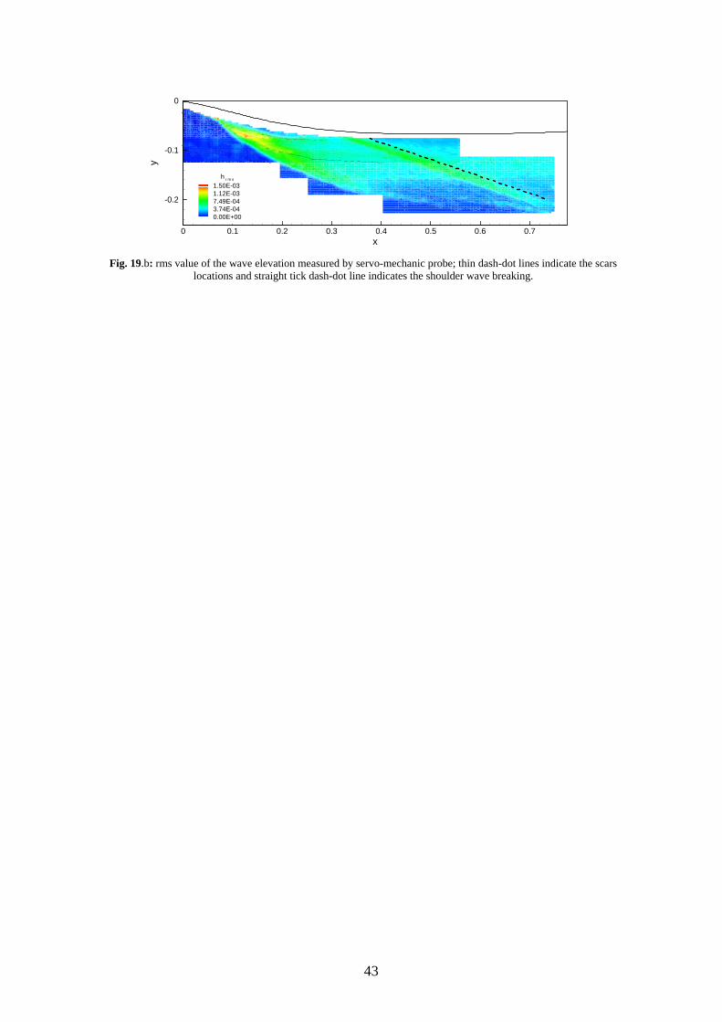
about 1/10 of the maximum wave height = 1.97 10-3 LPP (= 11.3 mm). The
shoulder wave breaking (spilling-type) is gentler than the bow wave breaking, as
underlined by the contours of the rms values of the wave fluctuation (fig.19.b).
(max)rmsh
The analysis of the mean wave field reveals some peculiar features of the
breaking. The bow wave (figs. 19.a and 20.a) displays a quite bumpy shape. The wave
front breaks into three regions separated by two scars, as observed in the photo study
17

(figs. 13 and 14). These scars are characterized by sudden changes in the mean wave
height. The first one (scar 2), closer to the hull, is more visible whereas the second
(scar 1), further from the hull, appears weaker as shown in Fig. 14b and beyond which
there is a region characterized by high free surface turbulence. Their location is
indicated in figures 19.a and 19.b and figures 20.a and 20.b, where the mean value and
the rms value of the wave height are shown together with the transverse wave cuts
used for the wave pattern reconstruction. The two scars are both characterized by
relatively high values of the wave fluctuations as shown in figure 20.b, where the rms
value of the wave elevation is shown.
Figures 21 and 22 show the velocity measurements under the bow wave in
terms of axial velocity contours and cross flow vectors (figs 21.a and 22.a) and axial
vorticity contours (21.b and 22.b).
Figures 21.a and 21.b relate to cross section x = 0.15. Axial velocity defect
under the bow wave crest is noticed in correspondence of high cross flow (fig. 21.a).
Clockwise (negative) vorticity is present under the breaking bow wave. A small region
of positive (counterclockwise) vorticity is also shown nearby the scar 1 (fig. 21.b).
Unfortunately, due to the dimension of the 5-hole Pitot head and the unsteadiness of
the free surface, it was not possible to reach the free surface in order to complete the
velocity field, and part of the vorticity dynamics is missing in the present analysis.
Figures 22.a and 22.b relate to cross section x = 0.20. As for section x = 0.15,
the flow at section x = 0.20 exhibits an axial velocity defect under the bow wave crest
in correspondence of high cross flow (fig. 22.a). The vorticity pattern is also very
similar to x = 0.15, although positive vorticity is observed here, under the clockwise
(negative) vortex (fig. 22.b). As for section x = 0.15, the measurements could not reach
the free surface and not all the vorticity is highlighted by present data. It is reasonable
to presume that positive vorticity has to be present close to the negative vorticity
region. To answer this question CFD results obtained by RANS code will be used to
complete the EFD data.
The dynamics of the shoulder wave breaking appears to be completely different
from the bow wave breaking. In particular, as shown by the picture in figure 14.d, the
shoulder wave breaking is spilling-type and the contours of the rms value of the wave
elevation in fig. 19.b show that in the near field the wave front develops along a
straight line inclined of about 19° with respect to the x-axis.
18

Figures 23.a and 23.b relate to cross section x = 0.40. Figure 23.a shows the
cross flow vectors and axial velocity contours under the shoulder wave crest, the bow
wave trough and part of the velocity field related to the bow wave crest (y < 0.16).
As for the bow wave crest, the axial velocity under the shoulder wave has a
local minimum, whereas, moving outboard, the axial velocity exhibits a local
maximum, in correspondence of the bow wave trough. The flow under the bow wave
crest (y < 0.16) is still characterized by low axial velocity, as for the upstream sections
x = 0.15 and x = 0.2.
Figure 23.b shows the axial vorticity patterns. Two clearly defined regions of
negative vorticity are visible under the shoulder wave crest (y = 0.085, z = 0.01) and
(y = 0.11, z = 0.01), while closer to the free surface a thin region of positive vorticity
is noticed (y = 0.09, z = 0.008). Moving outboard, very close the free surface, a thin
strip of negative vorticity is shown, which ends nearby the bow wave crest, where a
region of positive vorticity is observed (y = 0.195, z = 0.005).
Figures 24.a and 24.b show the flow pattern at x = 0.5. As for section x = 0.4
the axial velocity under the shoulder wave crest has a local minimum with high cross
flow close to the breaker. The flow under the bow wave trough shows a maximum of
the axial velocity (fig. 24.a).
The axial vorticity pattern shows two negative vortices located at (y = 0.085,
z = 0.01) and (y = 0.11, z = 0.01) as for section x = 0.4, whereas the positive vorticity
is visible at (y = 0.12, z = 0.06). It has to be mentioned that, although the closest
vectors to free surface were not used for the vorticity calculations, it is presumed that
the vorticity very close to the free surface could be affected by higher uncertainty than
in the rest of the measured field and some boundary effects could compromise the
results on the points close to the free surface.
The shoulder wave flow exhibits some similarities with a 2D spilling breaker,
although a fundamental difference occurs in the 3D scenario. In a 2D breaking, the
flow direction is normal to the wave front (aligned with the wave vector), whereas in
the present case the flow direction and the wave front form an angle of about 19°,
being the flow almost aligned with the x-axis. This difference likely does not affect the
mechanism responsible for the vorticity production at the toe of the wave breaking, but
it plays a fundamental role in the vorticity convection and evolution. Indeed, in a 2D
breaker the vorticity produced at the toe can only be convected downstream, normally
to the wave front generating a 2D shear layer. On the opposite, in the 3D case the
19

gradient of the velocity along the wave front can stretch the eddy generated at the
breaking. This mechanism can affect the vorticity intensity and consequently the
breaker intensity, whereas the propagation of the vorticity normal to the wave front is
very slow.
7. COMPLEMENTARY CFD OBSERVATIONS.
Concurrently to the described experimental campaign, a CFD simulation of the
same flow was carried out at IIHR using CFDSHIPIOWA RANS code, which is
described in details in [19].
Here, CFD data will be used to fill the EFD data in order to better understand
the flow under the bow and shoulder wave breaking, prior verification of the
agreement of the CFD results with EFD data in the measured regions. In fact, as
previously mentioned, it was not possible to measure very close to the free surface, due
to the free surface unsteadiness and dimensions of the Pitot head.
7.1. Free-Surface Wave Field and Flow.
A comparison of wave elevation contours with measurements at Fr = 0.35 is
provided in Figure 25, where the CFD prediction is able to capture the height of the
overturning bow and shoulder waves. The main differences are that the bow wave
height of the CFD prediction is underpredicted (i.e., the breaking is not as strong as in
the data) and the wavelength is shorter in comparison with the data. Figure 26 provides
a comparison of a photograph of the bow wave around the ship model and free-surface
perturbation streamlines from the CFD prediction (i.e., streamlines in an earth-fixed
coordinate system where the forward speed of the ship is subtracted from the axial
velocity). As indicated in the photograph, two “scars” on the free surface interface can
be observed (i.e., small-scale depressions in the free surface, which originate
downstream of the breaking bow wave and are aligned with the axial direction). The
location of the scars correlates with the location of the converging and diverging
perturbation streamline pattern in the CFD simulation. Figure 27 shows that the effect
of the trough in between the bow and shoulder waves (0.2 < x < 0.5) is to generate a
favorable pressure gradient normal to the trough line, which accelerates the axial flow
and turns the flow towards the hull giving the observed streamline pattern (i.e., axial
velocity greater than the free stream value and negative transverse velocity). It is this
20

sharp transition region, between the outward flow caused by the forebody and the
inward accelerating flow at the trough, which generates the diverging free surface
streamlines denoted as scar 1 in Figure 26. Downstream of the trough line, the flow
experiences an adverse pressure gradient and decelerates, eventually reversing sign as
seen at the shoulder wave in Figure 27 (i.e., the axial and transverse perturbation
velocity become negative and positive, respectively). The reversal of the perturbation
flow in between the trough and the shoulder wave results in a set of converging free
surface streamlines (denoted as scar 2 in Figure 26).
Although there is a correlation between the experimentally observed scars and
the perturbation streamlines, small scale depressions in the free-surface elevation are
not observed in the CFD simulations. Two possible explanations are that (i) the CFD
grid is very coarse in comparison to the scale of the scars and/or (ii) there is no surface
tension in the CFD calculations so we do not resolve the capillary waves on the free
surface.
As a matter of fact, even in the EFD wave elevation data, which measurement
grid is finer than the CFD grid, scars are not easy to recognize, especially downstream
the bow wave crest (x > 0.2). Additional research is required to determine the
mechanism for the generation of the scars. Future measurements and simulations may
be able to resolve the scars if the measurement and computational grids are extremely
fine.
7.2. Boundary Layer and Free-Surface Vortices.
Here, the CFD results are shown in terms of axial velocity and vorticity
contours at the four experimentally investigated cross sections x = 0.15, x = 0.20,
x = 0.40 and x = 0.50. The used code is able to accurately predict the “wake” of the
low speed fluid at the free surface downstream of the overturning bow wave (x = 0.15
and x = 0.20). Also, the acceleration of the axial velocity by the trough in between the
bow and shoulder wave is correctly predicted at x = 0.40 and x = 0.50. Comparisons of
the axial vorticity shows good agreement with experimental measurements with
respect to the magnitude, location, and content of the free surface vortices (Figs 28 a-d
and 29 a-d), giving also much more information on the flow very close to the free
surface.
21

Based on their good agreement with the EFD data, the CFD results can be used
to fill-in the sparse experimental dataset in order to understand the effects of the
overturning bow wave on the downstream flow.
To this purpose, free surface elevation and axial vorticity contours are shown in
figure 30 from CFD, where five free surface vortices are identified and labeled as
V1÷V5. The location of the vortex cores was found by tracing the center of closed
contours of axial vorticity from 0.1 < x < 0.6.
Form the whole field picture emerges that V1 and V4 are associated with the
overturning bow wave, while V2, V3, and V5 are associated with the shoulder wave.
It is clear that measurements are able only to highlight clearly V1 and V2,
while only traces of V4 and V5 can be recognized on figures 29 (a, b, c) and figures 29
(c, d) respectively.
Present work represents a good example of synergy between EFD and CFD. In
fact, we used EFD in order to validate CFD and successively CFD results in order to
fill-in the sparse experimental dataset, giving a complete picture of the analyzed flow.
8. A 3D BREAKING DETECTION CRITERION.
As observed in the photo study (fig. 14 d) and then measured (fig. 19.b), the
shoulder wave breaking closely resemble a 2D spilling breaking. As known by
literature (Duncan, [7]), the inception of 2D spilling breaking can be predicted based
on the ratio between wave amplitude and wavelength (2a/λ ≅ 0.1) of a regular wave
train. This criterion can be also expressed based on the related local steepness
θ = 17.1° ± 1.2° [7].
This second form of the 2D criterion can be in principle extended to complex
3D wave fields as the one examined in the present study.
Here, the wave steepness was determined by derivative of the mean wave
elevation normal to the wave front and it is shown in figure 25 (top). In the figure only
the 0° and 17° contours are shown, in order to localize better the breaking regions
predicted by the criterion. In the bottom plot of fig. 25, the rms value of the wave
elevation is represented in order to highlight the breaking region.
The comparison of the two plots in figure 25 shows that the θ = 17° criterion
seems to predict correctly the inception of the breaking, suggesting the usefulness of
22
the extension of the “local form” of the 2D criterion to 3D wave fields, at least for
spilling breakers.
9. Conclusions and Future Work
This report represents an advanced example of how complementary EFD and
CFD can provide a powerful and advanced tool in analyzing complex industrial flows
by completing and validating each other.
The results of an experimental campaign performed in collaboration at
INSEAN, using INSEAN model 2340A (exact geosym of the DTMB 5415) and at
IIHR, using DTMB model 5512 (3.038 m, 1/46.6 scale geosym of 5415) are reported.
The project was aimed at measuring 3D wave breaking generated by a fast
displacement surface combatant. The purpose was to provide detailed EFD data for
appropriate physics understanding as well as model development and CFD validation.
A careful photo study proved to be of great help in fixing the test conditions
(Fr = 0.35) and in putting in evidence some peculiar features of the free-surface flow,
namely “scars”. Mean and rms values for the near field wave elevations were
measured, whereas the far field was reconstructed with mean values only. Velocity
measurements under the bow and shoulder waves were conducted in four transversal
sections and the axial vorticity contours were also reconstructed, highlighting vortex
structures near the free-surface (WB vortices).
CFD simulations were used to complete the experimental data, allowing to give
a complete picture of the flow field under bow and shoulder waves and to identify
free-surface scars through the use of free-surface streamlines.
Present experimental data are among the most accurate and detailed
measurements of this type of flow and the authors believe that they will be of
relevance in CFD benchmarking. The analysis carried out demonstrated the richness of
the flow field under breaking waves. Current developments and future work include
more detailed computations in the free surface breaking region, making using of level
set approaches (to deal with large deformation and breaking of the free surface) and
chimera or overlapping grids for fine grid resolution.
From the experimental standpoint, the role of scale effects and surface tension
still need to be investigated beyond the present point. To this aim F. Pistani dedicated
his Ph.D. thesis [21] to measuring the flow field about a very large model of the 5415.
23
The scale adopted (λ=14.32, for a model length of Lpp=9.916 m) is sufficiently large
for the model divergent wave system to be negligibly affected by the surface tension
forces. At the moment the thesis is almost completed and the authors of the present
report believe that these data will represent a useful integration of the data reported
here and will help in further understanding ship breaking wave flows.
24
REFERENCES
1. OLIVIERI, A., PISTANI, F., AVANZINI, G., STERN, F. AND PENNA, R. 2001;
Towing Tank Experiments of Resistance, Sinkage and Trim, Boundary Layer,
Wake and Free Surface Flow around a naval combatant INSEAN 2340 Model.
IIHR Report No. 421.
2. LONGUET-HIGGINS, M.S., 1996; Progress towards understanding how waves
break. 21st Symposium on Naval Hydrodynamics, Trondheim, Norway.
3. OLIVIERI, A., PISTANI, F., AND PENNA, R. 2003; Experimental investigation of
the flow around a fast displacement ship hull model. J. Ship. Res, 47, 3 pp.247-
261.
4. COLEMAN, H.W., STEELE, W.G., 1995; Engineering Application of
Experimental Uncertainty Analysis. AIAA Journal, 33, 10, 1888-1895.
5. AVANZINI, G. PENNA, R., 1996; INSEAN Internal Report
6. DUNCAN, J. H., 2001; Spilling Breakers Ann. Rev. Fluid Mech, vol. 33.
7. DUNCAN, J. H., 1983; The breaking and non-breaking wave resistance of a
two-dimensional hydrofoil, J. Fluid Mech., vol. 126, pp. 507-520.
8. TENNEKES, H. LUMLEY, J. L., 1972; A first course in turbulence, Cambridge,
MA, U.S.A.: MIT Press.
9. DONG R.R., KATZ J., HUANG T.T., 1997; On the structure of Bow Waves on a
Ship Model, J. Fluid Mech., vol. 346, pp. 77-115
10. ROTH G. I, MASCENIK D. T., KATZ J., 1999; Measurements of the flow structure
and turbulence within a ship bow wave, Physics of Fluids n. 11,
vol. 11
11. LARSSON L., BABA, E. 1996; Ship resistance and flow computations Advances
in Marine Hydrodynamics, vol.5, Editor M. Ohkusu, CMP, Southampton,
Boston.
12. TROIANI G., 2004; Free Surface Turbulence: an experimental study at low
Reynolds numbers, PhD. thesis, Università “La Sapienza”, Roma.
13. http://www.chesapeakebay.net/info/ecoint3a.cfm
14. BONMARIN P., 1989; Geometric properties of deep-water breaking waves,
J. Fluid Mech., vol. 209, pp.405-433
25

15. TULIN M.P., LANDRINI M., 2000; Breaking waves in the ocean and around
ships, 23rd ONR Symposium on Naval Hydro., Val de Reuil (France).
16. TULIN M.P., 1996; Breaking of ocean waves and downshifting, Waves and
Nonlinear Processes in Hydrodynamics, Grue J., Gjevik B., Weber J.E. eds., pp
177-190, Kluwer Acad. Press.
17. STERN F., LONGO J., PENNA R., OLIVIERI A., RATCLIFFE T., COLEMAN H.,
2000; International collaboration on benchmark CFD validation data for
surface combatant DTMB model 5415, 23rd ONR Symposium on Naval
Hydro., Val de Reuil (France).
18. FU, T. C., KARION, A., RICE, R. J., WALKER, D. C., 2004; Experimental study of
the bow wave of the R/V Athena I, 25th ONR Symposium on Naval Hydro, St.
John’s, Canada.
19. WILSON, R., CARRICA, P., HYMAN, M., and STERN F., 2004; A single-phase
level set method with application to breaking waves and forward speed
diffraction problem, 25th ONR Symposium on Naval Hydro, St. John’s,
Canada.
20. LONGO J., STERN F., 2002; Effects of drift angle on model ship flow,
Experiments in Fluids, 32, 558-69.
21. PISTANI F., 2005; “Influence of large scale breaking waves in the near field of
ships”, Ph.D. Thesis, University of Rome La Sapienza, in preparation.
26
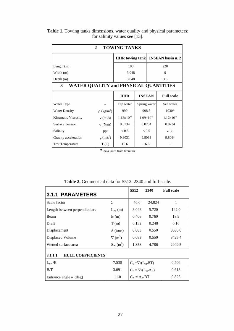
Table 1. Towing tanks dimensions, water quality and physical parameters; for salinity values see [13].
2 TOWING TANKS
IIHR towing tank INSEAN basin n. 2
Length (m) 100 220
Width (m) 3.048 9
Depth (m) 3.048 3.6
3 WATER QUALITY and PHYSICAL QUANTITIES
IIHR INSEAN Full scale
Water Type − Tap water Spring water Sea water
Water Density ρ (kg/m3) 999 998.5 1030*
Kinematic Viscosity ν (m2/s) 1.12×10⁻⁶ 1.09×10⁻⁶ 1.17×10⁻⁶
Surface Tension σ (N/m) 0.0734 0.0734 0.0734
Salinity ppt < 0.5 < 0.5 ≈ 30
Gravity acceleration g (m/s2) 9.8031 9.8033 9.806*
Test Temperature T (C) 15.6 16.6 -
* data taken from literature
Table 2. Geometrical data for 5512, 2340 and full-scale.
3.1.1 PARAMETERS 5512 2340 Full scale
Scale factor λ 46.6 24.824 1
Length between perpendiculars LPP (m) 3.048 5.720 142.0
Beam B (m) 0.406 0.760 18.9
Draft T (m) 0.132 0.248 6.16
Displacement ∆ (tons) 0.083 0.550 8636.0
Displaced Volume ∇ (m3) 0.083 0.550 8425.4
Wetted surface area SW (m2) 1.358 4.786 2949.5
3.1.1.1 HULL COEFFICIENTS
LPP /B 7.530 CB =∇/(LPPBT) 0.506
B/T 3.091 CP = ∇/(LPPAX) 0.613
Entrance angle α (deg) 11.0 CX = AX/BT 0.825
27
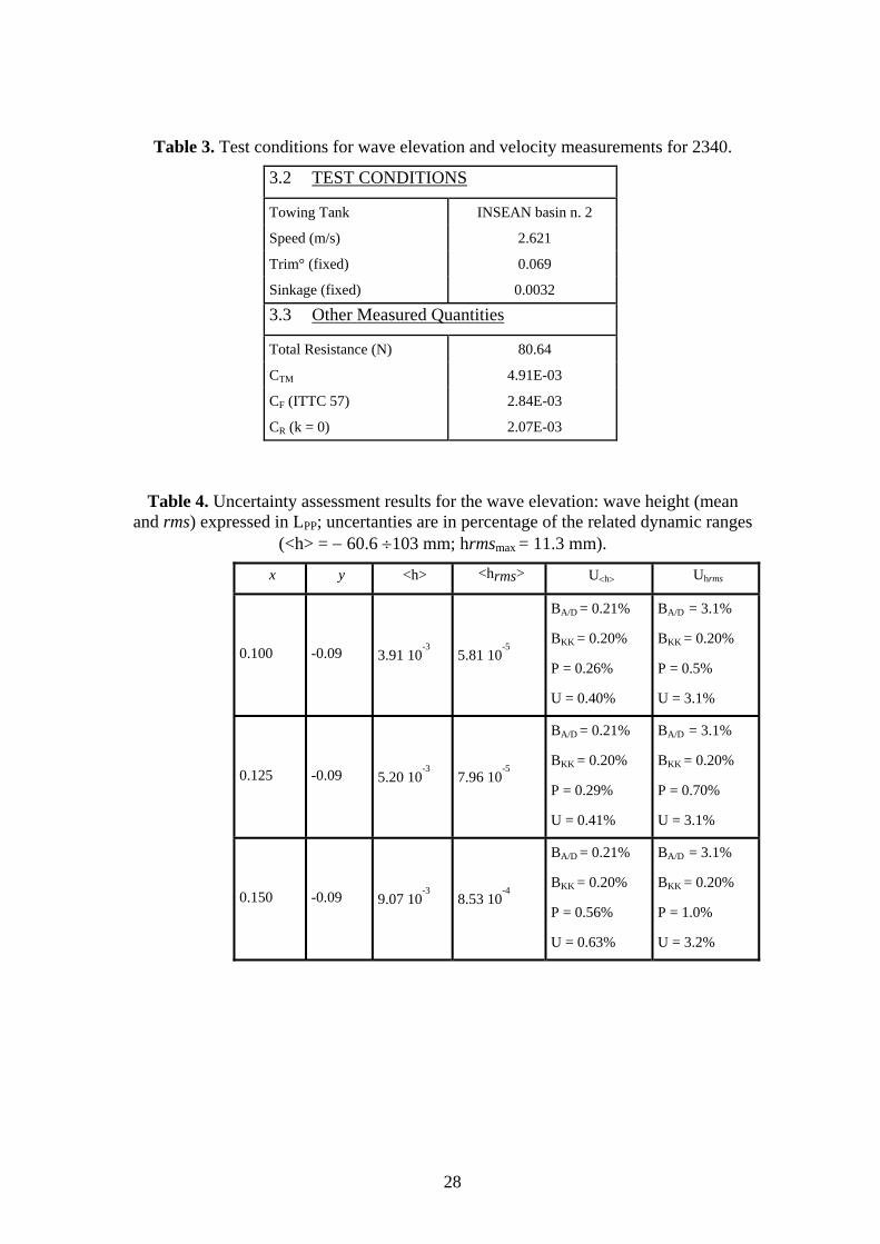
Table 3. Test conditions for wave elevation and velocity measurements for 2340.
3.2 TEST CONDITIONS
Towing Tank INSEAN basin n. 2
Speed (m/s) 2.621
Trim° (fixed) 0.069
Sinkage (fixed) 0.0032
3.3 Other Measured Quantities
Total Resistance (N) 80.64
CTM 4.91E-03
CF (ITTC 57) 2.84E-03
CR (k = 0) 2.07E-03
Table 4. Uncertainty assessment results for the wave elevation: wave height (mean and rms) expressed in LPP; uncertanties are in percentage of the related dynamic ranges
(<h> = − 60.6 ÷103 mm; hrmsmax = 11.3 mm).
x y <h> <hrms> U<h> Uhrms
0.100 -0.09 3.91 10-3
5.81 10-5
BA/D = 0.21%
BKK = 0.20%
P = 0.26%
U = 0.40%
BA/D = 3.1%
BKK = 0.20%
P = 0.5%
U = 3.1%
0.125 -0.09 5.20 10-3
7.96 10-5
BA/D = 0.21%
BKK = 0.20%
P = 0.29%
U = 0.41%
BA/D = 3.1%
BKK = 0.20%
P = 0.70%
U = 3.1%
0.150 -0.09 9.07 10-3
8.53 10-4
BA/D = 0.21%
BKK = 0.20%
P = 0.56%
U = 0.63%
BA/D = 3.1%
BKK = 0.20%
P = 1.0%
U = 3.2%
28

Table 5. Uncertainty assessment results for the three velocity components at the measuring point (x = 0.20, y = - 0.1015, z = - 0.005); U* = 2.621 m/s for the axial velocity component, while, for transverse and vertical components U*
corresponds to their range of variation in the measured field. < u > < v > < w >
Velocity 2.45 m/s
0.94 U0
-0.33 m/s
-0.12 U0
0.06 m/s
0.02 U0
Uncertainty B = 1.99 10-2 m/s
P = 8.04 10-3 m/s
Unc. = 2.15 10-2 m/s
Unc./U* = 0.82 %
B = 9.62 10-3 m/s
P = 2.59 10-3 m/s
Unc. = 9.96 10-3 m/s
Unc./U* = 1.63 %
B = 9.52 10-3 m/s
P = 9.38 10-4 m/s
Unc. = 9.56 10-3 m/s
Unc./U* = 1.56 %
Table 6. Non-dimensional parameters for 5512, 2340 and full scale.
Fr
U 5512
(m/s) U 2340
(m/s) U full scale
(m/s) U full scale
knots
We 5512
We 2340
We full scale
Re 5512
Re 2340
Re full scale
0.28 1.531 2.097 10.450 20 312 585 14800 4.17×10⁶ 1.10×10⁷ 1.27×10⁹
0.3 1.640 2.246 11.197 22 334 627 15800 4.46×10⁶ 1.18×10⁷ 1.36×10⁹
0.325 1.777 2.434 12.130 24 362 679 17100 4.83×10⁶ 1.27×10⁷ 1.47×10⁹
0.35 1.913 2.621 13.063 25 390 731 18400 5.21×10⁶ 1.37×10⁷ 1.59×10⁹
0.375 2.050 2.808 13.996 27 418 783 19800 5.58×10⁶ 1.47×10⁷ 1.70×10⁹
0.41 2.241 3.070 15.303 30 456 856 21600 6.10×10⁶ 1.61×10⁷ 1.86×10⁹
0.45 2.460 3.370 16.795 33 501 940 23700 6.69×10⁶ 1.76×10⁷ 2.04×10⁹
Table 7. Physical quantities for 5512, 2340 and full scale.
IIHR INSEAN full scale
g (m/s2) 9.8031 9.8033 9.81
ρ (kg/m3) 999 998.5 1030
ν (m2/s) 1.12E-06 1.09E-06 1.17E-06
σ (N/m) 0.0734 0.0734 0.0734
salinity < 0.5ppt < 0.5ppt ≈ 30ppt
29
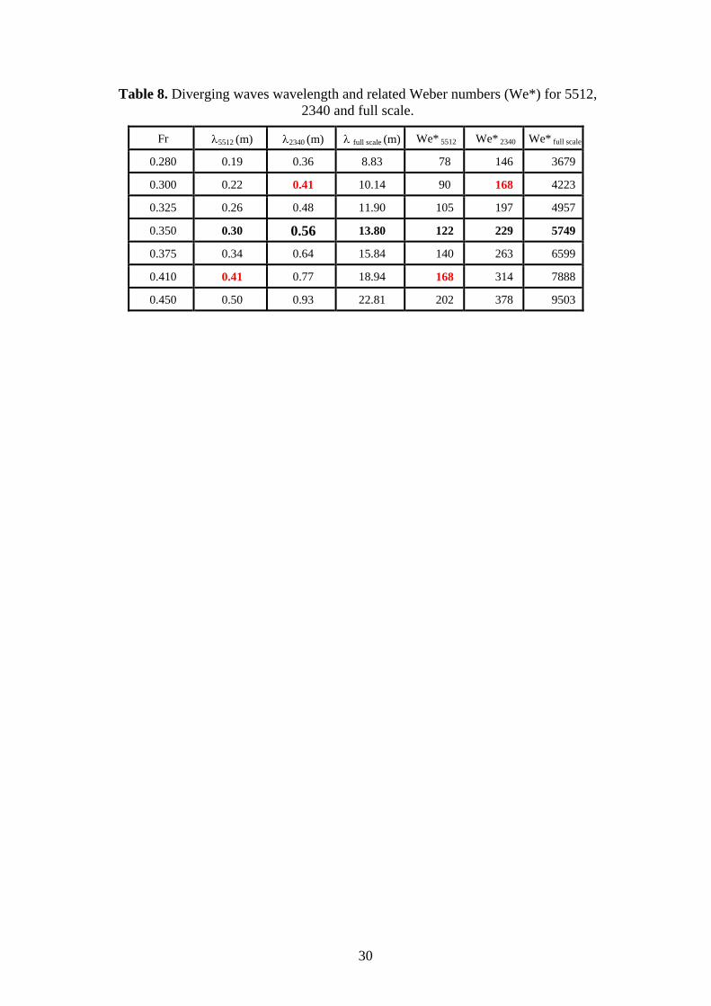
Table 8. Diverging waves wavelength and related Weber numbers (We*) for 5512, 2340 and full scale.
Fr λ5512 (m) λ2340 (m) λ full scale (m) We* 5512 We* 2340 We* full scale
0.280 0.19 0.36 8.83 78 146 3679
0.300 0.22 0.41 10.14 90 168 4223
0.325 0.26 0.48 11.90 105 197 4957
0.350 0.30 0.56 13.80 122 229 5749
0.375 0.34 0.64 15.84 140 263 6599
0.410 0.41 0.77 18.94 168 314 7888
0.450 0.50 0.93 22.81 202 378 9503
30

Fig. 1. INSEAN basin N.2: the carriage.
Fig. 2. IIHR towing tank
31
t (s)
h(m
m)
1 2 3 4-25
-20
-15
-10
-5
0
5
10
15
20
25
time hirunning meanrunning rms
Fig. 5. Breaking wave height signal time history and running mean and rms (x = 0.15, y = -0.09); the asymptotic
mean (<h> = 5.39 mm) has been subtracted to the running mean in the figure. The dash dot line represents the chosen acquisition time for the wave height acquisitions.
x
y
0 0.1 0.2 0.3 0.4 0.5 0.6 0.7 0.8 0.9 1 1.1
-0.4
-0.3
-0.2
-0.1
0
Measured area by finger probe (mean and rms)
Measured area by capacitance wires (mean)
Fig. 6. Measured area by finger probe and capacitance wires.
33
t(s)
p(k
Pa)
0 5 10 15 201
2
3
4
<Hc> (t)<Hp> (t)<Hc>asymptotic<Hp>asymptotic
Fig. 7. Central and Port pressure ports running mean for a measurement point located under the breaking. The dash
dot line represents the chosen acquisition time for the velocity acquisitions under the breaking.
y
z
-0.2 -0.18 -0.16 -0.14 -0.12 -0.1 -0.08 -0.06
-0.04
-0.03
-0.02
-0.01
0
0.01x = 0.50
a
y
z
-0.2 -0.18 -0.16 -0.14 -0.12 -0.1 -0.08 -0.06
-0.04
-0.03
-0.02
-0.01
0
0.01x = 0.50
b
Fig. 8. Measurement grid at x = 0.5: a) designed grid; b) properly acquired points.
34

a b
d c
f e
Fig. 13. Fr=0.35: 5512 side and front view (a, b); 2340 side and front view (c, d); full scale side and front view
(e, f ).
38

a b
c d
Fig. 15. Fr=0.375: 5512 side and front view (a, b); 2340 side and front view (c, d)
b a
d c
Fig. 16. Fr=0.41: 5512 side and front view (a, b); 2340 side and front view (c, d)
40

x
y
0 0.1 0.2 0.3 0.4 0.5 0.6 0.7
-0.2
-0.1
0
h r m s
1.50E-031.12E-037.49E-043.74E-040.00E+00
Fig. 19.b: rms value of the wave elevation measured by servo-mechanic probe; thin dash-dot lines indicate the scars
locations and straight tick dash-dot line indicates the shoulder wave breaking.
43
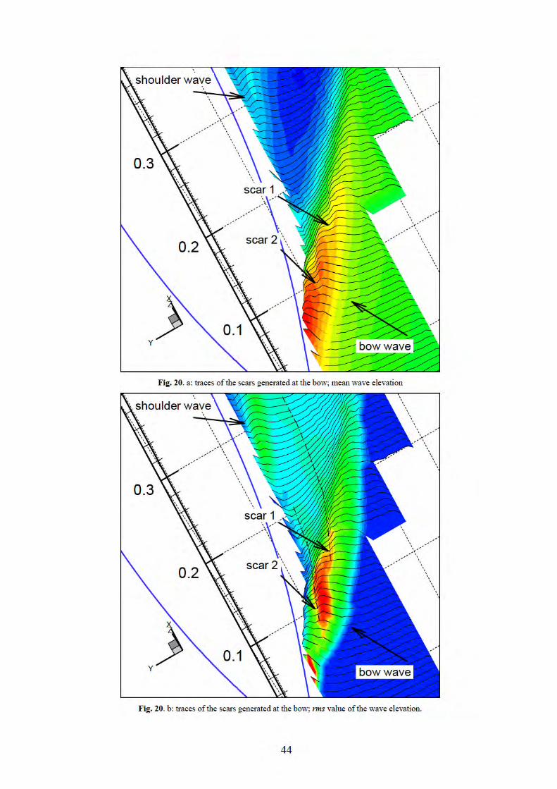

Fig. 21. x = 0.15: cross flow vectors and axial velocity contours (left); axial vorticity contours (right); arrow on top
left represents the undisturbed velocity; data on the right side obtained mirroring data on the left side.
45
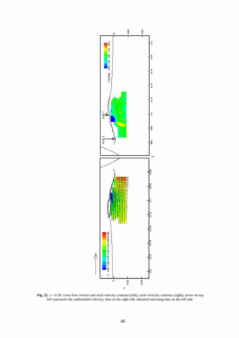
Fig. 22. x = 0.20: cross flow vectors and axial velocity contours (left); axial vorticity contours (right); arrow on top
left represents the undisturbed velocity; data on the right side obtained mirroring data on the left side.
46
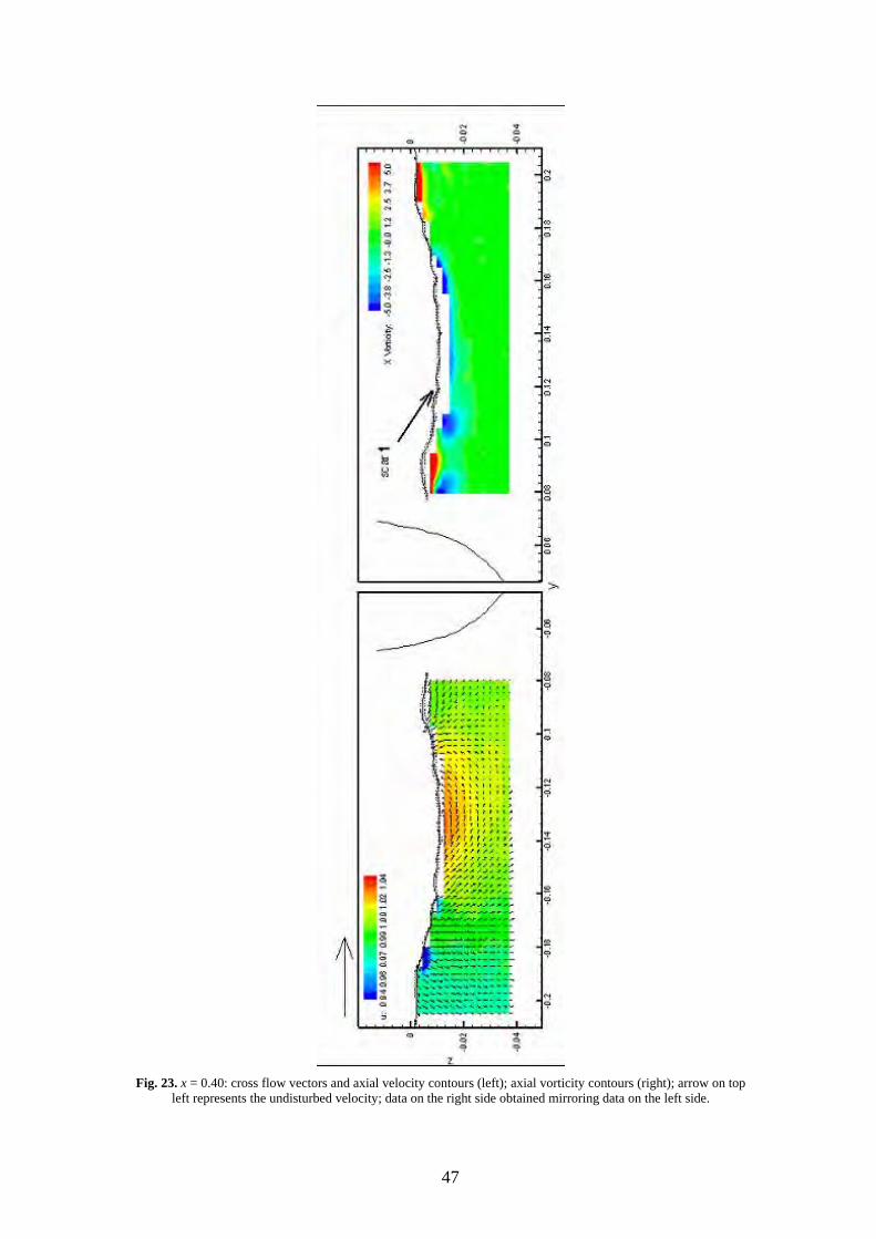
Fig. 23. x = 0.40: cross flow vectors and axial velocity contours (left); axial vorticity contours (right); arrow on top
left represents the undisturbed velocity; data on the right side obtained mirroring data on the left side.
47
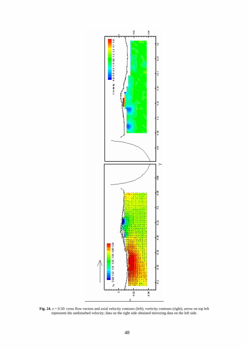
Fig. 24. x = 0.50: cross flow vectors and axial velocity contours (left); vorticity contours (right); arrow on top left represents the undisturbed velocity; data on the right side obtained mirroring data on the left side.
48

Fig. 25 Free surface contours for the surface combatant in calm water.
Fig. 26 scars and perturbation surface streamlines: picture taken during experiments (top); IIHR CFD [19]
(bottom).
49

Fig. 27 Trough detail of free-surface contours and perturbation streamlines.
50
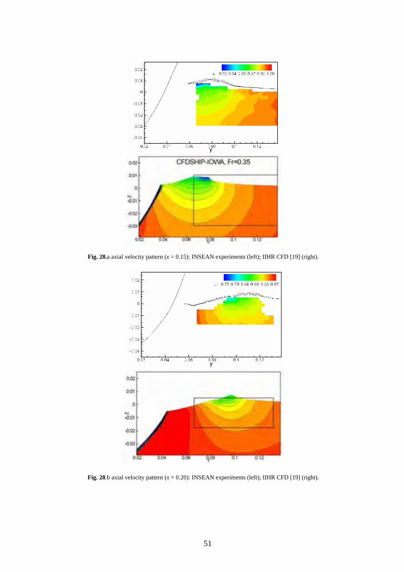
Fig. 28.a axial velocity pattern (x = 0.15): INSEAN experiments (left); IIHR CFD [19] (right).
Fig. 28.b axial velocity pattern (x = 0.20): INSEAN experiments (left); IIHR CFD [19] (right).
51
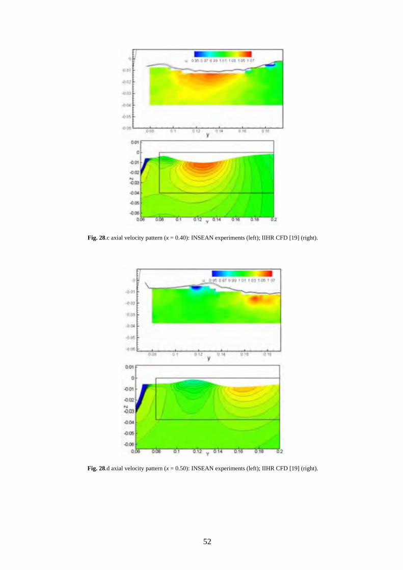
Fig. 28.c axial velocity pattern (x = 0.40): INSEAN experiments (left); IIHR CFD [19] (right).
Fig. 28.d axial velocity pattern (x = 0.50): INSEAN experiments (left); IIHR CFD [19] (right).
52
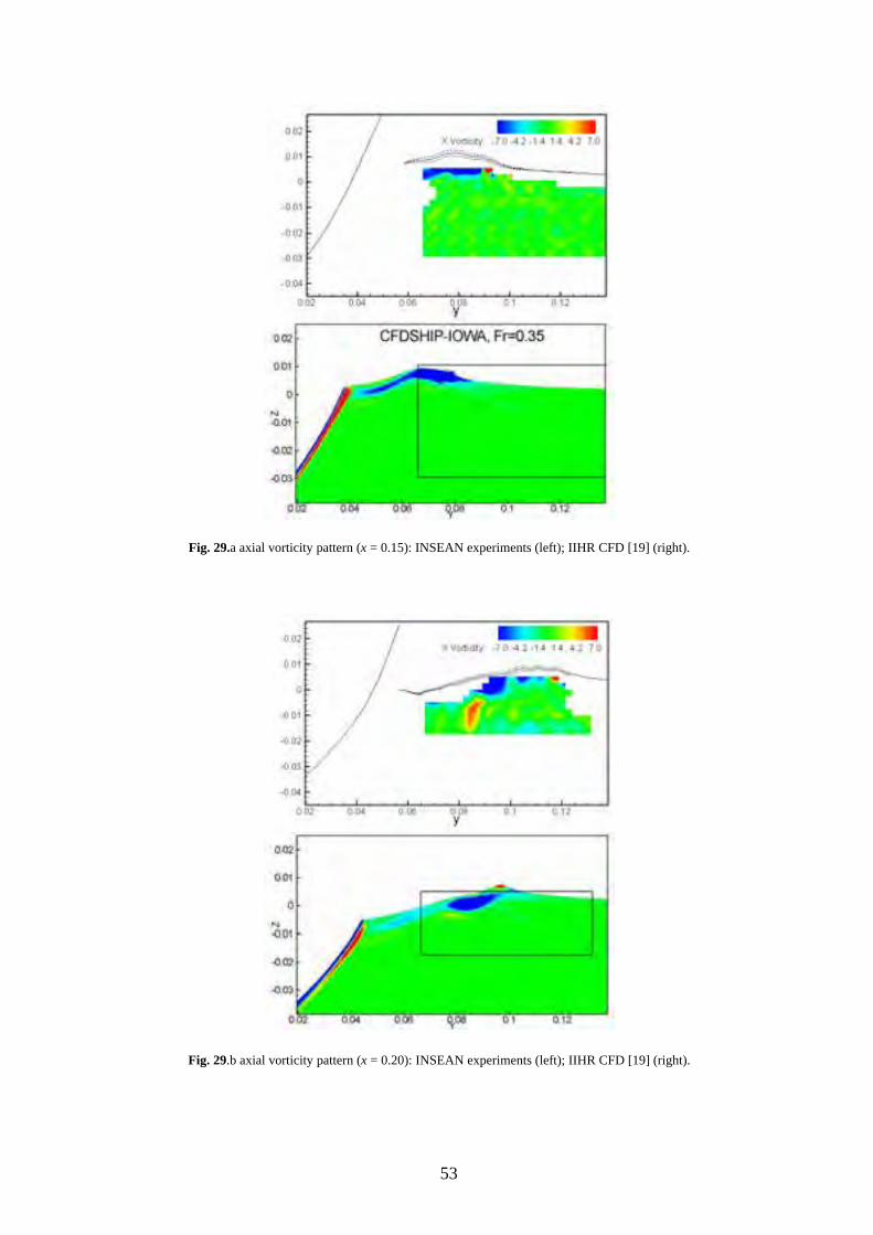
Fig. 29.a axial vorticity pattern (x = 0.15): INSEAN experiments (left); IIHR CFD [19] (right).
Fig. 29.b axial vorticity pattern (x = 0.20): INSEAN experiments (left); IIHR CFD [19] (right).
53

Fig. 29.c axial vorticity pattern (x = 0.40): INSEAN experiments (left); IIHR CFD [19] (right).
Fig. 29.d axial vorticity pattern (x = 0.50): INSEAN experiments (left); IIHR CFD [19] (right).
54

Fig. 30.Under free surface perspective of wave contours (background flood) and axial vorticity (slices)
55

Top Related