


Languages
Pages
Legal


Forecasting COVID-19 with Gamma Model
by
Zhenyao Tang
A thesis submitted in partial fulfilment
of the requirement for the degree of
Master of Science (M.Sc.) in Computational Sciences
The Faculty of Graduate Studies
Laurentian University
Sudbury, Ontario, Canada
©Zhenyao Tang, 2020

THESIS DEFENCE COMMITTEE/COMITÉ DE SOUTENANCE DE THÈSE
Laurentian Université/Université Laurentienne
Faculty of Graduate Studies/Faculté des études supérieures
Title of Thesis
Titre de la thèse Forecasting COVID-19 with Gamma Model
Name of Candidate
Nom du candidat Tang, Zhenyao
Degree
Diplôme Master of Science
Department/Program Date of Defence
Département/Programme Computational Sciences Date de la soutenance août 17, 2020
APPROVED/APPROUVÉ
Thesis Examiners/Examinateurs de thèse:
Dr. Waldemar W. Koczkodaj
(Supervisor/Directeur(trice) de thèse)
Dr. Dominik Strzalka
(Committee member/Membre du comité)
Approved for the Faculty of Graduate Studies
Approuvé pour la Faculté des études supérieures
Dr. David Lesbarrères
Monsieur David Lesbarrères
Dr. Richard Hurley Dean, Faculty of Graduate Studies
(External Examiner/Examinateur externe) Doyen, Faculté des études supérieures
ACCESSIBILITY CLAUSE AND PERMISSION TO USE
I, Zhenyao Tang, hereby grant to Laurentian University and/or its agents the non-exclusive license to archive and
make accessible my thesis, dissertation, or project report in whole or in part in all forms of media, now or for the
duration of my copyright ownership. I retain all other ownership rights to the copyright of the thesis, dissertation or
project report. I also reserve the right to use in future works (such as articles or books) all or part of this thesis,
dissertation, or project report. I further agree that permission for copying of this thesis in any manner, in whole or in
part, for scholarly purposes may be granted by the professor or professors who supervised my thesis work or, in their
absence, by the Head of the Department in which my thesis work was done. It is understood that any copying or
publication or use of this thesis or parts thereof for financial gain shall not be allowed without my written
permission. It is also understood that this copy is being made available in this form by the authority of the copyright
owner solely for the purpose of private study and research and may not be copied or reproduced except as permitted
by the copyright laws without written authority from the copyright owner.

Abstract
COVID-19 is a highly contagiously atypical pneumonia attributed to a novel coro-
navirus. The global economy and people's lives have been tremendously a�ected
by the COVID-19 pandemic since its outbreak in Wuhan, Hubei province, China.
In this thesis, a non-linear model based on gamma distribution was built to verify
the accuracy of the forecasting of the total con�rmed cases of COVID-19 two weeks
ahead. The daily growth in cases of COVID-19 for di�erent countries was monitored
and compared with the forecasted values. The veri�cation of the performance of the
non-linear Gamma distribution model has been veri�ed by the non-linear regression.
The data for the 19 countries with the most total con�rmed COVID-19 cases as of
June 22 was used. The data was sourced from the interactive web-based dashboard
developed by the Center for System Science and Engineering (CSSE) at Johns Hop-
kins University. A web page has been developed to provide predictions generated by
our models for individuals and public organizations to forecast the trends of COVID-
19.
Keywords
Forecasting, forecasting veri�cation, COVID-19, World Health Organization, WHO,
Gamma distribution, non-linear regression, dashboard prototype, jQuery
2

Acknowledgement
Foremost, I would like to express my sincere gratitude to my supervisor Prof. Walde-
mar Koczkodaj for formulating my master's study and research with the topic that
forecasting COVID-19 with nonlinear algorithmic models. Whenever I need help,
he always supports me. His guidance has been indispensable to me throughout the
entire process.
Furthermore, I would like to acknowledge Dr. E. Kozlowski. He helped me a lot with
R code development. This was very helpful to me, since I was a novice R developer
when I started to write this thesis.
Last but not the least, I owe sincere and earnest gratitude to my parents: Guohong
Tang and Xianghong Ma. They have always supported me spiritually throughout
my life.
3

Contents
1 Introduction 9
1.1 COVID-19 Pandemic . . . . . . . . . . . . . . . . . . . . . . . . . . . 9
1.2 Gamma Distribution . . . . . . . . . . . . . . . . . . . . . . . . . . . 10
1.3 Contributions . . . . . . . . . . . . . . . . . . . . . . . . . . . . . . . 13
2 Related Work 15
2.1 COVID-19 Pandemic the Growing Phase Forecasting . . . . . . . . . 15
2.2 Prediction of COVID-19 Cases . . . . . . . . . . . . . . . . . . . . . . 17
2.3 Approach Used in This Thesis . . . . . . . . . . . . . . . . . . . . . . 19
3 Dataset 20
3.1 Data Sources . . . . . . . . . . . . . . . . . . . . . . . . . . . . . . . 20
3.2 Data Identi�cation . . . . . . . . . . . . . . . . . . . . . . . . . . . . 23
3.3 Data Preprocessing . . . . . . . . . . . . . . . . . . . . . . . . . . . . 27
3.3.1 Data Construction for Prediction Model . . . . . . . . . . . . 28
3.3.2 Saving the Result of Predction Model . . . . . . . . . . . . . . 29
3.3.3 Data Construction for Data Visualization . . . . . . . . . . . . 31
3.4 Data Inaccuracy . . . . . . . . . . . . . . . . . . . . . . . . . . . . . . 33
4 Nonlinear Algorithmic Models 35
4.1 Basic Analysis of Original Data . . . . . . . . . . . . . . . . . . . . . 35
4.2 Basic Gamma Model . . . . . . . . . . . . . . . . . . . . . . . . . . . 48
4.3 Application of Gamma Distribution . . . . . . . . . . . . . . . . . . . 58
4

4.4 Analysis of Models . . . . . . . . . . . . . . . . . . . . . . . . . . . . 68
5 COVID-19 Pandemic Forecasting Web Page 92
6 Conclusion and Future Work 98
6.1 Conclusion . . . . . . . . . . . . . . . . . . . . . . . . . . . . . . . . . 98
6.2 Future Work . . . . . . . . . . . . . . . . . . . . . . . . . . . . . . . . 100
A Sample of Original Data 108
B Basic Gamma Prediction Model R Program 109
C Application Gamma Prediction Model R Program 118
5

List of Figures
Fig. 1 Probability density function plot of gamma distribution . . . . . . 12
Fig. 2 Cumulative distribution function plot of gamma distribution . . . 13
Fig. 3 COVID-19 Dashboard by CSSE at JHU . . . . . . . . . . . . . . . 21
Fig. 4 Commands of `RCurl' for downloading original data . . . . . . . . 22
Fig. 5 Codes to Generate Data for Prediction Model . . . . . . . . . . . . 28
Fig. 6 Codes to Save the Result of Prediction Model . . . . . . . . . . . . 29
Fig. 7 Codes to Construct Data for Data Visualization . . . . . . . . . . 32
Fig. 8 Total Con�rmed Cases of Top 19 Countries on June,22 . . . . . . . 35
Fig. 9 Real Daily Growth and Total Con�rmed Cases in the US . . . . . 37
Fig. 10 Real Daily Growth and Total Con�rmed Cases in Brazil . . . . . 38
Fig. 11 Real Daily Growth and Total Con�rmed Cases in Russia . . . . . 39
Fig. 12 Real Daily Growth and Total Con�rmed Cases in India . . . . . . 40
Fig. 13 Real Daily Growth and Total Con�rmed Cases in the United King-
dom . . . . . . . . . . . . . . . . . . . . . . . . . . . . . . . . . . . . 41
Fig. 14 Real Daily Growth and Total Con�rmed Cases in Peru . . . . . . 42
Fig. 15 Real Daily Growth and Total Con�rmed Cases in Spain . . . . . 43
Fig. 16 Real Daily Growth and Total Con�rmed Cases in Chile . . . . . . 45
Fig. 17 Real Daily Growth and Total Con�rmed Cases in Italy . . . . . . 46
Fig. 18 Real Daily Growth and Total Con�rmed Cases in Iran . . . . . . 47
Fig. 19 PDF of Gamma Distribution compared with Daily Growth . . . . 50
Fig. 20 CDF of Gamma Distribution compared with Total Con�rmed . . 52
6

Fig. 21 CDF of Gamma distribution compared with Total Con�rmed in
Iran . . . . . . . . . . . . . . . . . . . . . . . . . . . . . . . . . . . . 58
Fig. 22 PDF of Gamma Distribution Compared with Daily Growth in Iran 60
Fig. 23 PDF of Gamma Distribution Compared with Daily Growth in Iran 62
Fig. 24 Basic Gamma compared with Application Gamma . . . . . . . . 67
Fig. 25 Prediction Result of Basic Gamma Model of the US . . . . . . . . 69
Fig. 26 Prediction Result of Basic Gamma Model of Brazil . . . . . . . . 71
Fig. 27 Prediction Result of Basic Gamma Model of Russia . . . . . . . . 73
Fig. 28 Prediction Result of Basic Gamma Model of India . . . . . . . . . 75
Fig. 29 Prediction Result of Basic Gamma Model of UK . . . . . . . . . 77
Fig. 30 Prediction Result of Basic Gamma Model of Peru . . . . . . . . . 79
Fig. 31 Prediction Result of Basic Gamma Model of Spain . . . . . . . . 81
Fig. 32 Prediction Result of Basic Gamma Model of Chile . . . . . . . . . 83
Fig. 33 Prediction Result of Basic Gamma Model of Italy . . . . . . . . . 85
Fig. 34 Prediction Result of Application Gamma for Iran . . . . . . . . . 87
Fig. 35 Front End of the Home Page . . . . . . . . . . . . . . . . . . . . 93
Fig. 36 Front End of the Predict Page . . . . . . . . . . . . . . . . . . . . 95
Fig. 37 Process of the Back End of the COVID-19 Pandemic Forecasting
Web Page . . . . . . . . . . . . . . . . . . . . . . . . . . . . . . . . . 96
7

List of Tables
Tab. 1 Construction of Original Data . . . . . . . . . . . . . . . . . . . . 24
Tab. 2 Sample of the First Type of Data Construction . . . . . . . . . . . 25
Tab. 3 Sample of the Second Type of Data Construction . . . . . . . . . 26
Tab. 4 Sample of the Third Type of Data Construction . . . . . . . . . . 27
Tab. 5 Subset of One `data_cum' . . . . . . . . . . . . . . . . . . . . . . 30
Tab. 6 Subset of One `data_di�' . . . . . . . . . . . . . . . . . . . . . . . 31
Tab. 7 Example of One `plot_cum_data' or `plot_di�_data' . . . . . . . 33
Tab. 8 Total Con�rmed Cases of Top 19 Countries on June,22, 2020 . . . 36
Tab. 9 Prediction Inaccuracy Rate of the US . . . . . . . . . . . . . . . . 70
Tab. 10 Prediction Inaccuracy Rate of Brazil . . . . . . . . . . . . . . . . 72
Tab. 11 Prediction Inaccuracy Rate of Russia . . . . . . . . . . . . . . . 74
Tab. 12 Prediction Inaccuracy Rate of India . . . . . . . . . . . . . . . . 76
Tab. 13 Prediction Inaccuracy Rate of The United Kingdom . . . . . . . 78
Tab. 14 Prediction Inaccuracy Rate of Peru . . . . . . . . . . . . . . . . 80
Tab. 15 Prediction Inaccuracy Rate of Spain . . . . . . . . . . . . . . . . 82
Tab. 16 Prediction Inaccuracy Rate of Chile . . . . . . . . . . . . . . . . 84
Tab. 17 Prediction Inaccuracy Rate of Italy . . . . . . . . . . . . . . . . 86
Tab. 18 Prediction Inaccuracy Rate of Iran . . . . . . . . . . . . . . . . . 88
Tab. 19 Prediction Inaccuracy Rate of Top 19 Countries . . . . . . . . . 90
8

1 Introduction
1.1 COVID-19 Pandemic
In December 2019, a local outbreak of an atypical pneumonia occurred in Wuhan,
the capital city of Hubei province of China [1, 2]. It was quickly discovered to
be attributed to a novel coronavirus. The World Health Organization (WHO) has
termed it as Coronavirus Disease 2019 (COVID-19) [3]. An epidemiological link to
the Huanan Seafood Wholesale Market has been found as the source of the initial
cluster of cases [4]. Some typical symptomatic manifestations have been observed in
patients who are a�ected by COVID-19, including fever, cough, shortness of breath,
headache, confusion, muscle ache, chest pain, diarrhea and nausea and vomiting
[5, 6].
The annual period of mass migration called chunyun �associated with the Spring
Festival holidays� coincided with the outbreak. This enabled the outbreak to spread
rapidly to every province of China, with over 50,000 con�rmed cases and 1,000 deaths
cases reported domestically. While this was occurring, 603 cases were reported in
other countries and regions outside of China [7, 8].
This ongoing public health emergency has surpassed the severity of the 2003 outbreak
of severe acute respiratory syndrome (SARS), another atypical infectious pneumonia
[9]. As such, a series of unprecedented intervention strategies have been implemented
to contain the outbreak. For instance, cities have been quarantined, travel and public
9

gatherings strictly limited, public spaces shut down, and nationwide rigorous body
temperature monitoring has been implemented.
Since COVID-19 is highly contagious, the number of con�rmed cases in China in-
creased signi�cantly and rapidly. Due to this, on January 30, the WHO announced
that the event already constituted a Public Health Emergency of International Con-
cern [10]. The virus appeared quickly in countries outside of China due to inter-
national travel and transport, and the numbered of con�rmed cases grew rapidly
worldwide. All countries implemented strategies in order to contain the outbreak, in-
cluding early detection, maintenance of social distance, mask-wearing, active surveil-
lance, case management, and contact tracing. The global economy and people's lives
have been impacted tremendously by the COVID-19 pandemic.
1.2 Gamma Distribution
Gamma distribution is a two-parameter family of continuous probability distribu-
tions. The gamma distribution is the maximum probability distribution [11]. Ex-
ponential distribution, Erlang distribution, and chi-squared distribution are speci�c
types of gamma distribution, and are three di�erent parameterizations for the uti-
lization of gamma distribution. The �rst parameterization is composed of a shape
parameter k and a scale parameter θ. The second parameterization is composed of
a shape parameter α = k and an inverse scale parameter β = 1/θ, called a rate
parameter. Finally, the third parameterization is composed of a shape parameter
k and a mean parameter µ = kθ = α/β. In each of these three parameterizations,
10

all parameters are positive real numbers. In these three parameterizations, the �rst
parametrization k and θ is especially widely utilized in econometrics and other ap-
plied �elds. The implementation of gamma distribution is illustrated in [12].
A random variable X that exhibits gamma distribution with the shape K and scale
θ as its parameterization is denoted as:
X ∼ Γ(k, θ) ≡ Gamma(k, θ) (1− 1)
The probability density function of gamma distribution with the shape K and scale
θ as its parameterization is:
f(x; k, θ) =xk−1e− x
θ
θkΓ(k)forx > 0 and k, θ > 0 (1− 2)
Γ(k) is the gamma function evaluated at k, which is:
Γ(k) =
∫ ∞0
xk−1e−xdx ,<(k) > 0 (1− 3)
Figure 1 is taken from Wikipedia to illustrate the probability density function of
gamma distribution with the shape K and scale θas its parameterization:
11

Figure 1: Probability density function plot of gamma distribution
The cumulative distribution function of gamma distribution with the shape K
and scale θ as its parameterization is:
F (x; k, θ) =
∫ x
0
f(u; k, θ) =γ(k,
x
θ)
Γ(k)(1− 4)
The γ(k,x
θ) is the lower incomplete gamma function, which is:
γ(k,x
θ) =
∫ x
0
ts−1e−tdt (1− 5)
Figure 2 is taken from Wikipedia to illustrate the cumulative distribution function
of gamma distribution with the shape K and scale θ as its parameterization:
12

Figure 2: Cumulative distribution function plot of gamma distribution
Di�erent parameterizations of gamma distribution have di�erent implementations in
various situations. In this thesis, we chose the shape K and scale θ as the parame-
terization.
1.3 Contributions
The main contribution of this thesis is that we proposed a model to predict the total
con�rmed and daily con�rmed COVID-19 cases in di�erent countries with relatively
satisfactory accuracy. The core of our prediction algorithm is composed of gamma
distribution and nonlinear regression veri�cation of it. The model has two versions.
The simpler version with lower consumption of computing power was implemented
13

to predict most of countries. The advanced version with a higher consumption of
computing power was implemented to predict countries with more complex data.
Furthermore, we developed a web service online to provide information, including
the graph of real daily con�rmed cases, the graph of real total con�rmed cases, the
graph of predicted daily con�rmed cases, and the graph of predicted total con�rmed
cases. The corresponding predicted data over 14 days for the 19 countries that
have the most amount of total con�rmed cases was also shown. This information
can be useful to individuals as well as public organizations. Public organizations
will e�ciently allocate medical resources and publish policies to prevent the spread
of COVID-19. Individuals will get more information to help them make decisions
about their plans during the COVID-19 pandemic, i.e. cancelling large gatherings,
wearing masks, and/or limiting unnecessary travel. This thesis is of great importance
because predictions of COVID-19 can increase the awareness of society-at-large.
14

2 Related Work
2.1 COVID-19 Pandemic the Growing Phase Forecasting
In the twenty-�rst century, human beings have experienced several serious public
health events caused by pathogens shared with wild or domestic animals. These
include severe acute respiratory syndrome coronavirus (SARS-CoV), Middle East
Respiratory Syndrome coronavirus (MERS-CoV), and the in�uenza A (H1N1) virus
[18]. In order to control and prevent outbreaks and epidemics of infectious diseases,
numerous models have been designed within the epidemiologic �eld. Since the Out-
break of COVID-19, various prediction models have been implemented to aid in the
comprehension of this virus.
It is important to identify the origin of the virus as well as its intermediate hosts.
The development of genome sequencing technology has contributed a great deal to-
wards the tracing of COVID-19. As is pointed out in[19], the noncoding �anks of
the viral genome can be used to di�erentiate the recognized four Betacoronavirus
subspecies through whole-genome sequence comparisons, which has implications for
rapid classi�cation of new viruses. The comparison between the numerous mam-
malian coronavirus sequences and the genomic sequence obtained from COVID-19
suggests that bats may be a natural reservoir for COVID-19 [20]; subsequently, Pan-
golins are potential intermediate hosts [21].
In the early stages of an outbreak, it is vital to gain an understanding of the trans-
15

missibility of the pathogen at hand. In the early stages of the COVID-19, the
transmission chain of the virus was not clear. Therefore, many researchers adopted
information from SARS and MERS, which are similar to COVID-19, to aid their
understanding of it. The article [22] suggests that con�rmed cases may have been
roughly under-reported from the 1st to the 15th of January 2020, due to comparisons
with SARS cases. The epidemic curve of COVID-19 in mainland China from De-
cember 1, 2019 to January 24, 2020 had also been built by the exponential growth
Poisson process. They estimated the R0 of COVID-19 to be 2.56, and the number
of unreported cases to be 469, which has helped us understand what might have
happened in the early stages of outbreak.
While super-spreading events remains rare, they can cause large and explosive trans-
mission events and destroy hopes of successful prevention e�orts. In the article
[23], the researchers generated secondary cases for each primary case according to a
negative-binomial o�spring distribution with the mean R0 and dispersion k. After
1000 stochastic simulations for each individual combination, their simulations sug-
gested that very low values of k are less likely, and the establishment of sustained
transmission chains from single cases cannot be ruled out. Therefore, the importance
of screening, surveillance, and control e�orts cannot be ignored.
There are numerous other predictions in the epidemiologic �eld which can help people
understand COVID-19 from a medical perspective. Since this thesis focused on
prediction of COVID-19 cases, we are not going to introduce other predictions within
16

the epidemiologic �eld.
2.2 Prediction of COVID-19 Cases
Since the outbreak of COVID-19, many researchers have built various models to
predict the number of COVID-19 cases. These models have di�erent advantages and
disadvantages, and they provide di�erent methods and perspectives to help people
predict the number of cases.
In [24], the researchers successfully predicted that there would be over 1,000,000
COVID-19 cases outside of China by March 31st, 2020. The data is sourced from
the WHO situation report, in order to avoid risking data from an individual country
being biased or politically motivated. The model is based on assumption exponen-
tial growth of the pandemic. The coe�cients of exponential growth are estimated
by nonlinear regression analysis and the least squares method. The coe�cient a is
estimated at 10.4791 and the coe�cient b is estimated at 0.161. The model is simple
and easily explained. The error is 1.29%, which is acceptable for a short-term pre-
diction model.
In [25], the researchers built a model to predict the trend of COVID-19 in Wuhan,
Beijing, Shanghai and Guangzhou, four of the biggest cities in China. SEIR (Sus-
ceptible, Exposed, Infectious, Recovered) and neural networks (NNs) were used to
build the model. The data was composed of real-time data of COVID-19 in addition
to population mobility data. The time series data for COVID-19 by location, in-
17

cluding the number of con�rmed cases, deaths, recovered cases, and newly diagnosed
cases, was extracted from the website Tencent News. The population migration data
was extracted from �Baidu migration�, which is an open-source big data project.
According the results of the model, the researchers make the conclusion that the
COVID-19 epidemic in China has been e�ectively contained, and that the national
medical service is going to recover by April. However, they stated that the potential
for asymptomatic virus carriers still cannot be ignored.
The researchers in [26] built a model to predict the trend of the COVID-19 in China
based on the public health interventions. A modi�ed Susceptible-Exposed-Infections-
Removed (SEIR) model along with arti�cial intelligence (AI) were used to estimate
the curve of the epidemic. The data sources were composed of data from COVID-
19 and SARS. The epidemiological data from COVID-19 was extracted from the
National Health Commission of China. The 2003 SARS epidemic data between
April and June 2003 across China was retrieved from the SOHU News website. The
SARS epidemic data was then used to train the AI model. According to the results
of the model, the researchers predicted that the peak of the epidemic in China would
be February and that a gradual decline would appear in April. They also predicted
that a second epidemic peak might appear in Hubei province in the middle of March,
if the quarantine of Hubei province was suspended. Lastly, they predicted that if the
implementation of prevention measures in China were to have been delayed by �ve
days, the size of the epidemic would have been three times larger.
18

The researchers in [27] built a model for the early warning of some notable infectious
diseases in China. Real-time recurrent learning (RTRL) and EKF (Kalman �lter)
were used to build the model. The numbers of new con�rmed cases of eight types of
infectious diseases, reported per month between January 2004 and December 2015,
were extracted from the Center for National Public Health Scienti�c Data and the
National Health Commission websites. The model from this article can e�ectively
provide early warnings for some infectious diseases.
2.3 Approach Used in This Thesis
In this thesis, the core part of our model was selected as gamma distribution with
shape K and scale θ for parameterization. Furthermore, two gamma distributions
were combined to handle data from countries with complex patterns of daily report-
ing. In order to calculate the coe�cients of our model, nonlinear regression was used
to �t the given data, which was the total con�rmed cases and daily con�rmed cases
of di�erent countries. During the process, the least square method was used to �gure
out the most �tted coe�cients. More speci�c information about our model will be
introduced in the chapter 4.
19

3 Dataset
3.1 Data Sources
Since the outbreak of COVID-19, di�erent countries and public organizations have
collected and reported COVID-19 data, the WHO [28] and the Chinese Center for
Disease Control and Prevention [29] being two of those entities. It was di�cult to
�nd a dataset that was able to aggregate all of these data sources.
On January 22, 2020, an interactive web-based dashboard [30] was developed by the
Center for System Science and Engineering (CSSE) at Johns Hopkins University in
Baltimore, MD, USA. It was able to visualize and track reported cases of COVID-19
in real time. The dashboard is available online at [31]. It illustrates the location
and number of con�rmed COVID-19 cases, deaths, and recoveries for all a�ected
countries, as well as provides a global hot spot map of COVID-19 and other sta-
tistical information related to COVID-19. It is a user-friendly tool for individuals,
researchers, and public health authorities to learn about the COVID-19 pandemic.
COVID-19 cases are reported at di�erent levels depending on the region and coun-
try. Cases are reported at the provincial level in China, at the city level in the USA,
Australia and Canada, and at the country level in many other countries and regions.
The home page of the online dashboard is shown in �gure 3:
20

Figure 3: COVID-19 Dashboard by CSSE at JHU
The data collection period was divided into two parts. From January 21, 2020 to
January 31, all collection and processing of data was done manually. The data was
typically updated twice daily. After February 1, 2020, a semi-automated system of
collection was adopted. Before the online dashboard data was updated, the case
numbers were checked with the centers for disease control and prevention in China,
Taiwan, and Europe, as well as the Hong Kong Department of Health, the Macau
Government, the WHO, state-level health authorities in the U.S., the US CDC, the
government of Canada, the Australian Government Department of Health, and vari-
ous state or territory health authorities. Furthermore, the dashboard is particularly
21

e�ective at capturing the timing of the �rst reported cases of COVID-19 in new
countries and regions. Due to all of this, we were con�dent that this dashboard is a
suitable data source for this thesis. More importantly, the data from this dashboard
is freely available at GitHub [32].
Our original data was downloaded using an R package: `RCurl'. RCurl is a free and
open source R Package developed to transfer data. The commands from `RCurl' we
used to download our original data directly from GitHub is as follows:
Figure 4: Commands of `RCurl' for downloading original data
All of the data processing and analysis in this thesis were implemented by R [33]. R is
a programming language and free software environment for statistical computing and
22
graphics supported by the R Foundation for Statistical Computing [34, 35, 36]. The
R language is widely used in statistics, data mining, and statistical software. In the
scholarly research �eld, the applications of R increase substantially [37]. The o�cial
R software environment with command line interface is a GNU package which is
developed mainly in C, Fortran, and R itself. In this thesis, we used RStudio, which
is an integrated development environment for R. R is an implementation of the S
programming language and was created by Ross Ihaka and Robert Gentleman at
the University of Auckland, New Zealand. Since R is an open source programing
language, it contains almost all of the popular algorithm packages used in statistics
and data analysis.
3.2 Data Identi�cation
Since the data source is continuously updating, we adopted the data from June, 21,
2020 to use for this thesis. The dataset illustrated in this thesis is composed of 266
observations with 156 variables. The construction of the original data is as shown in
table 1:
23

Table 1: Construction of Original Data
Name Data Type
Province/State VARCHAR(50)
Country/Region VARCHAR(50)
Lat FLOAT
Long FLOAT
1/22/20 INT
1/23/20 INT
1/24/20 INT
. . . INT
6/21/20 INT
The name of the �rst row is `Province/State', which describes the location of this
observation at the provincial or state level. The name of the second row is `Coun-
try/Region', which describes the location of this observation at the country or re-
gional level. The name of the third row is `Lat', which describes the latitude value of
this observation. The name of the fourth row is `Lon', which describes the longitude
value of this observation. The names of the other rows are the dates, from January,
22, 2020 to June,21,2020. These rows describe the total con�rmed cases of COVID-
19 at this speci�c location on each corresponding date.
As we mentioned before, in the online COVID-19 dashboard, cases are reported
at di�erent levels depending on the di�erent region and country. In the original
24

data, observations were divided into three constructions. The �rst type of data
construction was designed for China and Canada. A sample of the �rst type of data
construction is as shown in table 2:
Table 2: Sample of the First Type of Data ConstructionProvince/State Country/Region Lat Long 1/22/20 1/23/20 6/20/20 6/21/20
Anhui China 31.8257 117.2264 1 9 991 991
Beijing China 40.1824 116.4142 14 22 821 830
Chongqing China 30.0572 107.874 6 9 582 582
Fujian China 26.0789 117.9874 1 5 363 363
Gansu China 37.8099 101.0583 0 2 151 151
Guangdong China 23.3417 113.4244 26 32 1634 1634
Guangxi China 23.8298 108.7881 2 5 254 254
Guizhou China 26.8154 106.8748 1 3 147 147
Hainan China 19.1959 109.7453 4 5 171 171
Hebei China 39.549 116.1306 1 1 344 346
Heilongjiang China 47.862 127.7615 0 2 947 947
Henan China 33.882 113.614 5 5 1276 1276
Hong Kong China 22.3 114.2 0 2 1128 1131
Hubei China 30.9756 112.2707 444 444 68135 68135
Hunan China 27.6104 111.7088 4 9 1019 1019
Inner Mongolia China 44.0935 113.9448 0 0 238 238
Jiangsu China 32.9711 119.455 1 5 653 653
Jiangxi China 27.614 115.7221 2 7 932 932
Jilin China 43.6661 126.1923 0 1 155 155
Liaoning China 41.2956 122.6085 2 3 153 154
In this �rst type of data construction, each observation describes the total con�rmed
number of COVID-19 cases in one province of one country on the corresponding date.
However, this is not designed to describe the total number of con�rmed COVID-19
cases in the whole country. Hence, in order to get results for the whole country,
we needed to sum the results of all the observations from the �rst type of data
construction.
25

The second type of data construction was designed for the United Kingdom and
France. A sample of the second type of data construction is as shown in table 3:
Table 3: Sample of the Second Type of Data ConstructionProvince/State Country/Region Lat Long 1/22/20 1/23/20 6/20/20 6/21/20
Bermuda United Kingdom 32.3078 -64.7505 0 0 146 146
Cayman Islands United Kingdom 19.3133 -81.2546 0 0 195 195
Channel Islands United Kingdom 49.3723 -2.3644 0 0 570 570
Gibraltar United Kingdom 36.1408 -5.3536 0 0 176 176
Isle of Man United Kingdom 54.2361 -4.5481 0 0 336 336
Montserrat United Kingdom 16.7425 -62.1874 0 0 11 11
Anguilla United Kingdom 18.2206 -63.0686 0 0 3 3
British Virgin Islands United Kingdom 18.4207 -64.64 0 0 8 8
Turks and Caicos Islands United Kingdom 21.694 -71.7979 0 0 12 14
Falkland Islands (Malvinas) United Kingdom -51.7963 -59.5236 0 0 13 13
United Kingdom 55.3781 -3.436 0 0 303110 304331
In the second type of data construction, most of the observations describe the total
con�rmed number of COVID-19 cases in one state of one country on the correspond-
ing date. There is also a metric designed to describe the total number of con�rmed
COVID-19 cases for the whole country. Thus, in order to get the results for the
whole country, we simply need to �nd the cell that is aligned with the value for
`Country/Region', and contains the given country's name.
The third type of data construction is designed for all other countries. A sample for
the second type of data construction is as shown in table 4:
26

Table 4: Sample of the Third Type of Data ConstructionProvince/State Country/Region Lat Long 1/22/20 1/23/20 6/20/20 6/21/20
Azerbaijan 40.1431 47.5769 0 0 12238 12729
Barbados 13.1939 -59.5432 0 0 97 97
Costa Rica 9.7489 -83.7534 0 0 2127 2213
Diamond Princess 0 0 0 0 712 712
Egypt 26 30 0 0 53758 55233
Fiji -17.7134 178.065 0 0 18 18
Germany 51 9 0 0 190670 191272
Haiti 18.9712 -72.2852 0 0 5077 5077
Iran 32 53 0 0 202584 204952
Japan 36 138 2 2 17725 17780
"Korea, South" 36 128 1 1 12421 12438
Kuwait 29.5 47.75 0 0 39145 39650
Lebanon 33.8547 35.8623 0 0 1536 1587
Malaysia 2.5 112.5 0 0 8556 8572
Nepal 28.1667 84.25 0 0 8605 9026
Oman 21 57 0 0 28566 29471
Peru -9.19 -75.0152 0 0 251338 251338
Qatar 25.3548 51.1839 0 0 86488 87369
Russia 60 90 0 0 576162 583879
Singapore 1.2833 103.8333 0 1 41833 42095
Turkey 38.9637 35.2433 0 0 186493 187685
Uganda 1 32 0 0 763 770
Vietnam 16 108 0 2 349 349
Zambia -15.4167 28.2833 0 0 1430 1430
In the third type of data construction, there is only one metric designed to describe
the number of total con�rmed COVID-19 cases for each country. Thus, we can easily
get the results for the whole country by �nding the cell that aligns with the value of
`Country/Region', and that contains the desired country's name.
3.3 Data Preprocessing
Analyzing data that has not been carefully screened for problems can produce mis-
leading results. Thus, the representation and quality of data is the �rst priority
27

before running an analysis [38]. Data cleaning, data integration, data reduction,
data transformation, and data discretization are common methods of data prepro-
cessing [39]. Even though the original data of this thesis is relatively clean and
well-organized, it is still unable to be used directly as data for our prediction model.
There are three main data preprocessing tasks in this thesis: constructing data for
the prediction model, saving the results of the prediction model, and constructing
data for data visualization.
3.3.1 Data Construction for Prediction Model
As we mentioned in chapter 3.2, the original data observations were divided into
three constructions. Therefore, we needed to deal with the di�erent constructions
in order to generate the data for our prediction model. The codes for accomplishing
this task is as follows:
Figure 5: Codes to Generate Data for Prediction Model
At the beginning of the code, the subset of the original data is generated based on the
name of the country or region. Then, according to the di�erent data constructions of
di�erent countries, the value for total con�rmed COVID-19 cases on di�erent dates in
28

the corresponding country are extracted to a vector named `country'. Then, a vector
named `x' is created with the same length as that of the vector named `country'.
These two vectors are then aggregated into a data frame.
3.3.2 Saving the Result of Predction Model
After the prediction model is generated, the prediction value from the prediction
model and the real value should be saved properly for the next step of data processing:
data visualization. The codes to accomplish this are as follows:
Figure 6: Codes to Save the Result of Prediction Model
At the end of these codes, a data frame named `data_cum' is generated to save
the real and predicted values for the number of total con�rmed COVID-19 cases on
di�erent dates of the corresponding country. Another data frame named `data_di�'
is generated to save the real and predicted values for the number of daily con�rmed
29
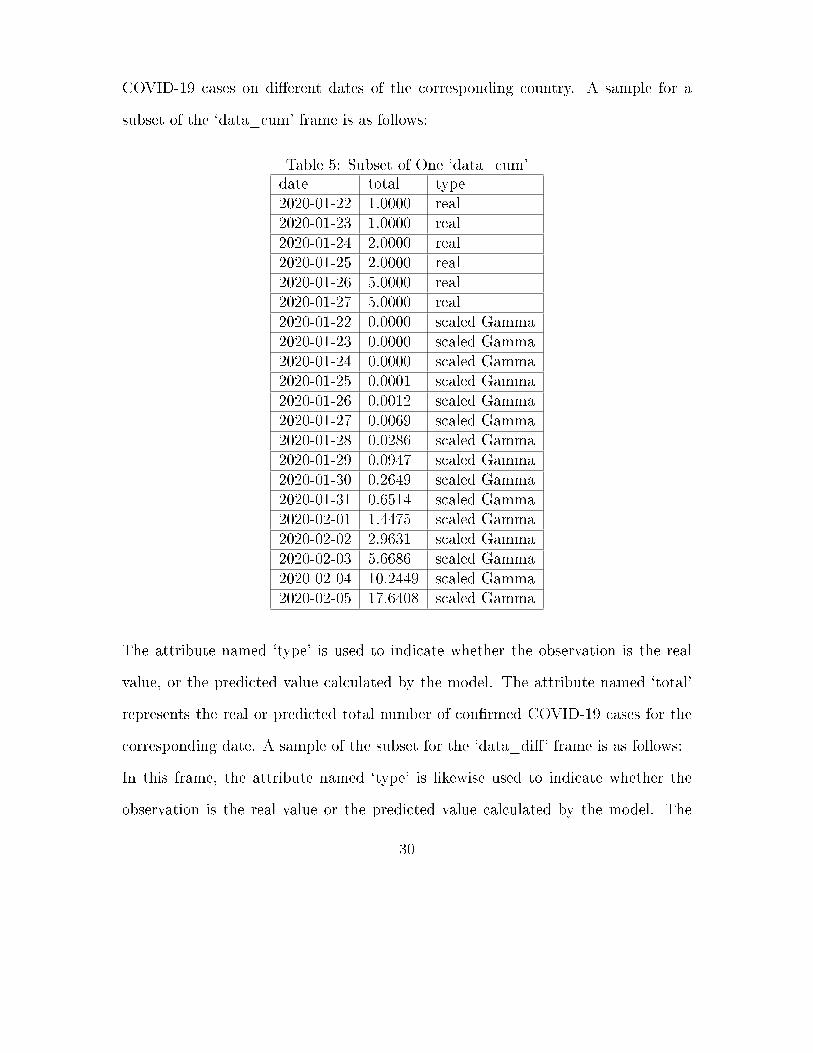
COVID-19 cases on di�erent dates of the corresponding country. A sample for a
subset of the `data_cum' frame is as follows:
Table 5: Subset of One `data_cum'date total type2020-01-22 1.0000 real2020-01-23 1.0000 real2020-01-24 2.0000 real2020-01-25 2.0000 real2020-01-26 5.0000 real2020-01-27 5.0000 real2020-01-22 0.0000 scaled Gamma2020-01-23 0.0000 scaled Gamma2020-01-24 0.0000 scaled Gamma2020-01-25 0.0001 scaled Gamma2020-01-26 0.0012 scaled Gamma2020-01-27 0.0069 scaled Gamma2020-01-28 0.0286 scaled Gamma2020-01-29 0.0947 scaled Gamma2020-01-30 0.2649 scaled Gamma2020-01-31 0.6514 scaled Gamma2020-02-01 1.4475 scaled Gamma2020-02-02 2.9631 scaled Gamma2020-02-03 5.6686 scaled Gamma2020-02-04 10.2449 scaled Gamma2020-02-05 17.6408 scaled Gamma
The attribute named `type' is used to indicate whether the observation is the real
value, or the predicted value calculated by the model. The attribute named `total'
represents the real or predicted total number of con�rmed COVID-19 cases for the
corresponding date. A sample of the subset for the `data_di�' frame is as follows:
In this frame, the attribute named `type' is likewise used to indicate whether the
observation is the real value or the predicted value calculated by the model. The
30

Table 6: Subset of One `data_di�'date growth type2020-01-23 0 real2020-01-24 1 real2020-01-25 0 real2020-01-26 3 real2020-01-27 0 real2020-01-28 0 real2020-01-21 0 scaled Gamma2020-01-22 0 scaled Gamma2020-01-23 0 scaled Gamma2020-01-24 0.0003 scaled Gamma2020-01-25 0.0023 scaled Gamma2020-01-26 0.0108 scaled Gamma2020-01-27 0.0372 scaled Gamma2020-01-28 0.1046 scaled Gamma2020-01-29 0.254 scaled Gamma2020-01-30 0.5507 scaled Gamma2020-01-31 1.0924 scaled Gamma2020-02-01 2.0164 scaled Gamma2020-02-02 3.5071 scaled Gamma2020-02-03 5.8027 scaled Gamma2020-02-04 9.2011 scaled Gamma
attribute named `growth' represents the real or predicted number of daily con�rmed
COVID-19 cases on the corresponding date.
3.3.3 Data Construction for Data Visualization
We used an R package named `Plotly' to visualize the results from our model. `Plotly'
is a free and open source R graphing library that makes interactive graphs suitable
for public use [40]. In order to utilize this package, we reconstructed the data to
meet the data structure requirement of `Plotly'. The codes used for this are shown
31

in �gure 7:
Figure 7: Codes to Construct Data for Data Visualization
At the end of these codes, a data frame named `plot_cum_data' is generated to
plot the curve of the real or predicted values for the total number of con�rmed
COVID-19 cases for each corresponding country. Additionally, a data frame named
`plot_di�_data' is generated to plot the curve of the real or predicted values for
the number of daily con�rmed COVID-19 cases for each corresponding country. A
sample of the subset for `plot_cum_data' and `plot_di�_data' are as follows:
The attribute named `scaled' represents the predicted daily or total con�rmed COVID-
19 cases for the corresponding date. The attribute named `real' represents the real
daily or total number of con�rmed COVID-19 cases for the corresponding date. The
reason that there are some `NA' values in the attribute named `real' is that we didn't
32

Table 7: Example of One `plot_cum_data' or `plot_di�_data'date scaled real2020-06-08 2072305.243 19617812020-06-09 2092653.896 19798682020-06-10 2112629.573 20007022020-06-11 2132231.892 20235902020-06-12 2151460.848 20489862020-06-13 2170316.804 20745262020-06-14 2188800.469 20940582020-06-15 2206912.89 21140262020-06-16 2224655.433 21377312020-06-17 2242029.77 21632902020-06-18 2259037.861 21910522020-06-19 2275681.943 22225792020-06-20 2291964.516 22551192020-06-21 2307888.323 22798792020-06-22 2323456.345 NA2020-06-23 2338671.779 NA2020-06-24 2353538.028 NA2020-06-25 2368058.69 NA2020-06-26 2382237.54 NA2020-06-27 2396078.522 NA2020-06-28 2409585.735 NA
have the real value for that corresponding date when we generated this data frame.
3.4 Data Inaccuracy
As we mentioned, the data source for the article [24] is the WHO situation report,
in order to mitigate the risk of data from an individual country being misreported
due to bias or politically motivation, reducing the overall accuracy of our data.
Furthermore, according to CNN [41], the Center for Disease Control and Prevention
announced that for every COVID-19 infection reported, there are ten more that have
33

gone undiagnosed. This implies that some level of inaccuracy is inevitable for any of
the data collected about COVID-19. In another words, it is relatively impossible to
�nd a data source that will represent the real state of COVID-19 with 100% accuracy.
34
4 Nonlinear Algorithmic Models
4.1 Basic Analysis of Original Data
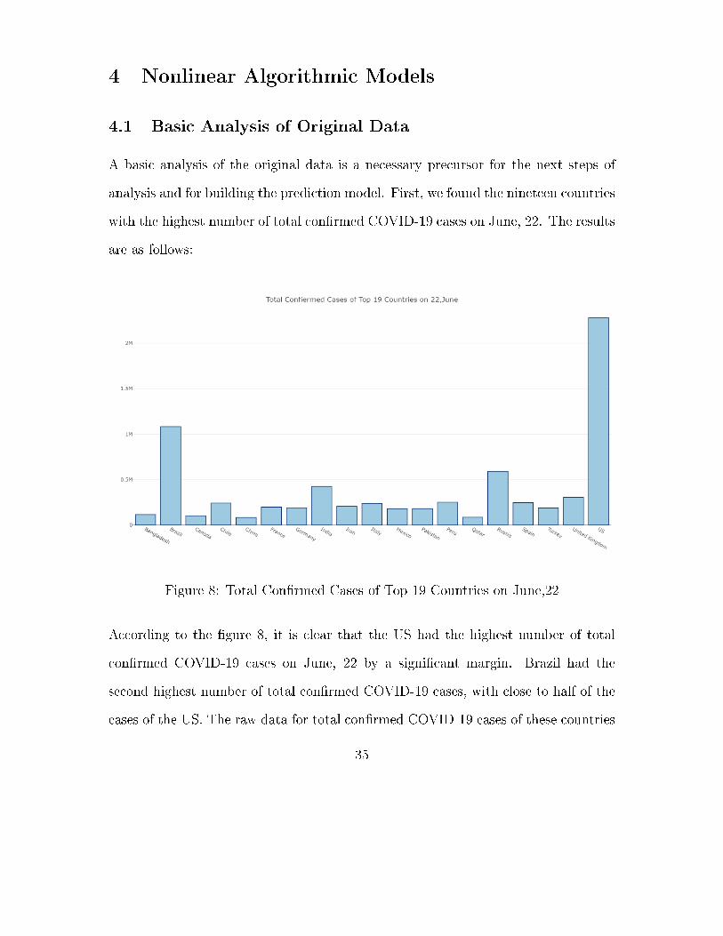
A basic analysis of the original data is a necessary precursor for the next steps of
analysis and for building the prediction model. First, we found the nineteen countries
with the highest number of total con�rmed COVID-19 cases on June, 22. The results
are as follows:
Figure 8: Total Con�rmed Cases of Top 19 Countries on June,22
According to the �gure 8, it is clear that the US had the highest number of total
con�rmed COVID-19 cases on June, 22 by a signi�cant margin. Brazil had the
second highest number of total con�rmed COVID-19 cases, with close to half of the
cases of the US. The raw data for total con�rmed COVID-19 cases of these countries
35

are as follows:
Table 8: Total Con�rmed Cases of Top 19 Countries on June,22, 2020Country June,22US 2280969Brazil 1083341Russia 591456India 425282United Kingdom 305803Peru 251338Spain 246272Chile 242355Italy 238499Iran 207525France 197008Germany 191668Turkey 187685Pakistan 181088Mexico 180545Bangladesh 115786Canada 103078Qatar 87369China 84573
It is helpful for us to identify these top 19 countries, as it allows us to assume that
there is enough valid data to build and train the prediction model using the data
of these countries. To verify that the data from these 19 countries has enough valid
values and diversi�ed distributions, we plotted a graph of the total con�rmed cases
and the daily growth in cases for the 10 countries with the most representative data
distribution. This graph is as follows:
36

Figure 9: Real Daily Growth and Total Con�rmed Cases in the US
Figure 9 illustrates the trends for daily growth in number of con�rmed cases, as well
as the cumulative total number of COVID-19 cases in the US. As is shown, the total
number of con�rmed COVID-19 cases in the US began to sharply increase in late
March, and the shape of the graph is close to a line with a positive slope. The daily
growth in number of COVID-19 cases in the US peaked for the �rst time in early
April, and then it started to �uctuate violently. Although the �uctuation in daily
growth was drastic, the lowest value was still just under 20,000, an extremely high
number. The graph indicates that the COVID-19 epidemic in the US was getting
worse as of June 22.
37

Brazil had the second-highest total number of con�rmed COVID-19 cases as of June,
22. The graph of total con�rmed cases and daily growth in cases in Brazil is as follows:
Figure 10: Real Daily Growth and Total Con�rmed Cases in Brazil
Figure 10 illustrates the trends of daily growth in number of cases, as well as the
cumulative total number of COVID-19 cases in Brazil, shown over time. As is shown,
the total number of con�rmed COVID-19 cases in Brazil started to increase gradually
on April 12th, and the shape of the graph is close to exponential growth. The daily
growth in number of COVID-19 cases in Brazil started to gradually increase on April
12th, with increasingly volatile �uctuations, and an upward trend on the whole. The
graph indicates that the COVID-19 epidemic in Brazil was getting worse as of June
22.
38
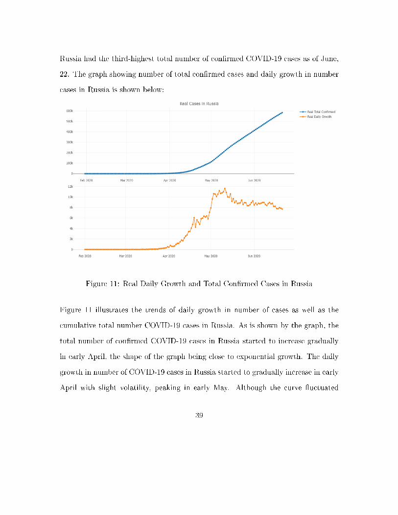
Russia had the third-highest total number of con�rmed COVID-19 cases as of June,
22. The graph showing number of total con�rmed cases and daily growth in number
cases in Russia is shown below:
Figure 11: Real Daily Growth and Total Con�rmed Cases in Russia
Figure 11 illustrates the trends of daily growth in number of cases as well as the
cumulative total number COVID-19 cases in Russia. As is shown by the graph, the
total number of con�rmed COVID-19 cases in Russia started to increase gradually
in early April, the shape of the graph being close to exponential growth. The daily
growth in number of COVID-19 cases in Russia started to gradually increase in early
April with slight volatility, peaking in early May. Although the curve �uctuated
39

slightly, it exhibited a downward trend after it peaked. The graph indicates that the
COVID-19 epidemic in Russia began to improve after peaking.
Furthermore, the graph of the total number of con�rmed cases and daily growth
cases in India is shown below:
Figure 12: Real Daily Growth and Total Con�rmed Cases in India
Figure 12 illustrates the trends in daily growth of COVID-19 cases, as well as the
cumulative total number of COVID-19 cases in India. As is shown by the, the total
number of con�rmed COVID-19 cases in India started to increase gradually in early
April, with the shape of the graph close to exhibiting exponential growth. The daily
growth in number of COVID-19 cases in India started to gradually increase in early
40

April, and continued growing afterwards with slight volatility. Although the curve
�uctuated slightly, it showed a continuous upward trend. The graph indicates that
the COVID-19 epidemic in India was getting worse as of June 22.
The graph showing total number of con�rmed cases and daily growth in number of
cases for the United Kingdom is shown below::
Figure 13: Real Daily Growth and Total Con�rmed Cases in the United Kingdom
Figure 13 illustrates the trends in daily growth of COVID-19 cases, as well as the
cumulative total number of COVID-19 cases, for the United Kingdom. As is shown
by the graph, the total number of con�rmed COVID-19 cases in the United Kingdom
started to increase gradually in late March, with the shape of the graph close to ex-
41

hibiting exponential growth. After that, the curve for the total number of con�rmed
cases �attens slightly after June. The daily growth in number of COVID-19 cases in
the United Kingdom started to sharply increase in the middle of March with slight
volatility, peaking shortly thereafter towards the middle of April. Although the curve
initially �uctuated violently, it showed a downward trend after peaking. The graph
indicates that the COVID-19 epidemic in the United Kingdom has been improving
after its peak.
The graph showing total number of con�rmed cases and daily growth in number of
cases in Peru is shown below:
Figure 14: Real Daily Growth and Total Con�rmed Cases in Peru
42

Figure 14 illustrates the trends in daily growth in number of COVID-19 cases, as
well as the cumulative total number of COVID-19 cases in Peru. As is shown by the
graph, the total number of con�rmed COVID-19 cases in Peru started to increase
gradually in late March, with the shape of the graph close to exhibiting exponential
growth. Furthermore, the daily growth in number of COVID-19 cases in Peru started
to sharply increase in the middle of March with volatility. The curve �uctuated with
increasing volatility, showing a continuous upward trend. The graph indicates that
the COVID-19 epidemic in the Peru has been getting worse.
The graph showing total number of con�rmed COVID-19 cases, as well as daily
growth in number of cases for Spain is shown below:
Figure 15: Real Daily Growth and Total Con�rmed Cases in Spain
43

Figure 15 illustrates the trends in daily growth in numbers of COVID-19 cases, as
well as the cumulative total number of COVID-19 cases in Spain. As is shown by the
graph, the total number of con�rmed COVID-19 cases in Spain began to increase
sharply in mid-March, with the shape of the graph close to exhibiting exponential
growth. Afterwards, the curve for the total number of con�rmed cases begins to
slightly �atten after May. The daily growth in number of COVID-19 cases in Spain
began to sharply increase in the middle of March with slight volatility, with its peak
in late March. Although the curve �uctuated violently, it showed a downward trend
after peaking. There was an obvious outlier in late April, the reason for which is
unclear. The graph indicates that the COVID-19 epidemic in Spain has been getting
better after peaking.
The graph showing the total number of con�rmed cases and the daily growth in
number of cases in Chile is shown below:
44
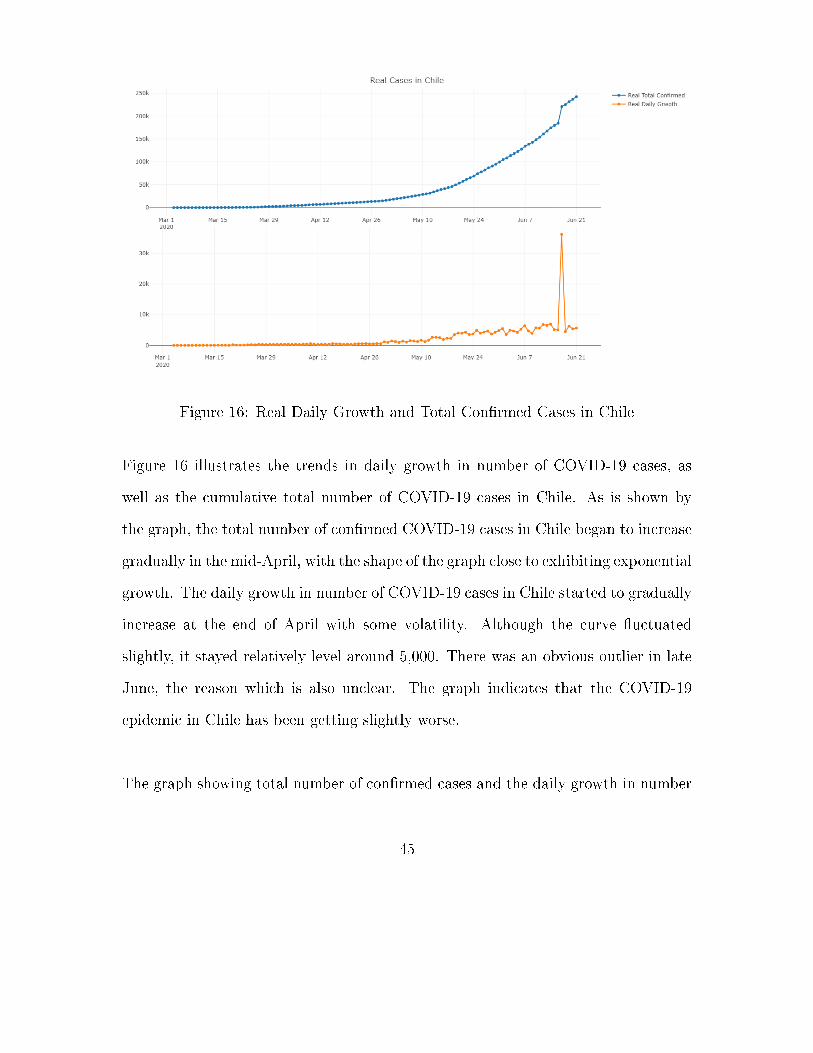
Figure 16: Real Daily Growth and Total Con�rmed Cases in Chile
Figure 16 illustrates the trends in daily growth in number of COVID-19 cases, as
well as the cumulative total number of COVID-19 cases in Chile. As is shown by
the graph, the total number of con�rmed COVID-19 cases in Chile began to increase
gradually in the mid-April, with the shape of the graph close to exhibiting exponential
growth. The daily growth in number of COVID-19 cases in Chile started to gradually
increase at the end of April with some volatility. Although the curve �uctuated
slightly, it stayed relatively level around 5,000. There was an obvious outlier in late
June, the reason which is also unclear. The graph indicates that the COVID-19
epidemic in Chile has been getting slightly worse.
The graph showing total number of con�rmed cases and the daily growth in number
45

cases for Italy is shown below:
Figure 17: Real Daily Growth and Total Con�rmed Cases in Italy
Figure 17 illustrates the trends in daily growth in number of COVID-19 cases, as
well as the cumulative total number of COVID-19 cases in Italy. As is shown by
the graph, the total number of con�rmed COVID-19 cases in Italy began to increase
sharply in the middle of March, with the shape of the graph close to exhibiting
exponential growth. The curve for the total number of con�rmed cases begins to
�atten in early May. The daily growth in number of COVID-19 cases in Italy started
to sharply increase in the middle of March with slight volatility, peaking in the middle
of April. Although the curve �uctuated violently, it showed a downward trend and
�nally hovered around zero. The graph indicates that the COVID-19 epidemic in
Italy has been getting better after peaking.
46

Lastly, the graph showing total number of con�rmed cases and daily growth in num-
ber cases for Iran is shown below:
Figure 18: Real Daily Growth and Total Con�rmed Cases in Iran
Figure 18 illustrates the trends in daily growth in number of COVID-19 cases, as
well as the cumulative total number of COVID-19 cases in Iran. As is shown by
the graph, the total number of con�rmed COVID-19 cases in Iran started to increase
sharply in late February, with the shape of the graph resembling a line with a positive
slope. Notably, it is apparent that there were two peaks in the curve for daily growth
in number of COVID-19 cases in Iran. This value peaked for the �rst time in late
March, and then gradually decreased until early May. After early May, the daily
growth in number of COVID-19 cases sharply increased once again, and peaked for
a second time in early June. After the second peak, daily growth in COVID-19 cases
47

remained at a stable level, and didn't show a downward trend. The graph indicates
that Iran had two peaks in the number of COVID-19 cases from February to June,
and that the COVID-19 epidemic in Iran has still been getting worse.
According to the basic analysis of the original data for the 10 countries with the
highest total number of cases, we can come to some conclusions. First, the trends
of total number of con�rmed COVID-19 cases for di�erent countries are generally
similar, and is either close to exponential growth or a line with a positive slope.
Using this, it is possible to build a model with a simple statistical core to estimate
the total number of con�rmed COVID-19 cases in di�erent countries. Second, the
distributions of the daily growth in number of COVID-19 cases in di�erent countries
are extremely di�erent. Thus, it is comparatively more di�cult to build a model
with a simple statistical core to estimate the daily growth in number of COVID-19
cases in di�erent countries. Third, the shape of the curve for the daily growth in
number of COVID-19 cases in Iran is totally di�erent from the other countries, since
it has two peaks. Therefore, estimating the daily growth in number of COVID-19
cases in Iran will probably require a more complex model.
4.2 Basic Gamma Model
After the analysis of the original data in the previous part, we started to consider the
mathematical core of our prediction model. We �rst compared the graphs showing
daily growth in number of COVID-19 cases in di�erent countries, and the graphs
showing the total number of con�rmed COVID-19 cases in di�erent countries, with
48

the plots for probability density functions and cumulative distribution functions of
various traditional statistical models. This was done in order to �nd some similar
patterns between them. After communicating with professor Sobocinski [42], we de-
cided to compare the two sets of graphs with plots of probability density function and
cumulative distribution functions of gamma distribution. The comparison between
the plots of daily growth in number of COVID-19 cases in �ve countries with the
plots of probability density function of gamma distribution is as follows:
49

Figure 19: PDF of Gamma Distribution compared with Daily Growth
50

This �gure illustrates the probability density function of gamma distribution and
the plots of daily growth in number of COVID-19 cases in the United Kingdom,
Spain, Italy, Germany, and Turkey. It is apparent that the plot of probability density
function of gamma distribution is extremely similar to the plots showing daily growth
in COVID-19 cases in these countries. This may indicate that they show similar
patterns.
The comparison between the plots showing the total number of con�rmed COVID-19
cases in �ve countries with the plots of cumulative distribution function of gamma
distribution is as follows:
51

Figure 20: CDF of Gamma Distribution compared with Total Con�rmed
52

This �gure illustrates the cumulative distribution function of gamma distribution
and the plots showing the total number of con�rmed COVID-19 cases in the United
Kingdom, Spain, Italy, Germany, and Turkey. From this, we can see that the plot
for cumulative distribution function of gamma distribution is quite similar with the
plots showing total con�rmed cases in these countries. This may also imply that
the two exhibit similar patterns. Based on these comparisons, we decided to use the
gamma distribution as the mathematical core for our prediction model.
53

The process for our Basic Gamma Prediction Model is as follows:
Basic Gamma Prediction
(1) Load data of COVID-19 dashboard by CSSE into the data frame.
(2) Data preprocess to generate trained data.
(3) Use R package nls and R function gamma() to �t the non-linear model to
data by computing a, b, and, c:
y = f(x) =a ∗ x(b−1) ∗ e−x
c
cb ∗ gamma(b)
(4) Compute the prediction of total con�rmed cases by the R function pgamma()
and plot the curve:
prediction = a ∗ pgamma(x, shape = b, scale = c)
(5) Compute the prediction of daily growth cases by the R function dgamma()
and plot the curve:
prediction = a ∗ dgamma(x, shape = b, scale = c)
In the �rst step of this process, the original data is loaded as a data frame into the
R environment in order to preprocess it for the next step.
In the second step, the original data is reconstructed to the form as the data for
54

regression.
In the third step, the R function gamma(b) is the gamma function evaluated at b,
which is:
gamma(b) =
∫ ∞0
xb−1e−xdx ,<(b) > 0 (4− 1)
In order to estimate the coe�cients of a, b and c in the gamma distribution, the
R function nls was utilized. According to [33], the Nonlinear Least Squares (nls)
calculates the nonlinear (weighted) least-squares estimates of the coe�cients in a
nonlinear model. An nls object is a type of �tted model object. It has methods
for the generic functions anova, coef, con�nt, deviance, df.residual, �tted, formula,
log-Lik, predict, print, pro�le, residuals, summary, vcov, and weights.
In the third step, we considered a non-linear model of the following form:
yi = f(xi; a, b, c) + εi, i = 1, ..., n (4− 2)
with the function f(.) of the form:
f(x) =a ∗ x(b−1) ∗ e−x
c
cb ∗ gamma(b)(4− 3)
From [43], we estimated the parameters a, b, and c by applying the non-linear least
squares method, in which the residual sum of squares was minimized.
55

Sn(a, b, c) =n∑i=1
[yi − f(xi; a, b, c)]2 (4− 4)
In this formula, the yi represents the number for the daily increase in COVID-19
cases in one country.
It is usually necessary to provide the initial values of the parameters in a non-linear
model when people are using nls, in order to avoid a convergence failure, which
is when the function evaluation limit is reached without convergence. As such, we
needed to estimate the initial values for parameters a, b, and c. The formulas and
variable relations, which helped us to estimate the initial values of parameters a, b,
and c, are as follows:
a = −ln(σ√
2π)− µ2
2σ2+ ln(k + ∆) (4− 5)
a∆ = −ln(σ√
2π)− µ2
2σ2(4− 6)
ln(k + ∆) = a− a∆ (4− 7)
b =µ
σ2− 1 (4− 8)
c = −(1
2σ2) (4− 9)
Here, µ is the expected value of the original data and σ is the standard deviation for
the original data.
56

In the fourth step of the process, the R function pgamma(x, shape = b, scale = c)
is the distribution function of gamma distribution where the value of the shape is b
and value of the scale is c. This is shown below:
F (x; b, c) =
∫ x
0
f(u; b, c) =γ(b,
x
c)
Γ(b)(4− 10)
Here the γ(b,x
cis the lower in complete gamma function:
γ(b,x
c) =
∫ x
0
ts−1e−tdt (4− 11)
In the �fth step, the R function dgamma(x, shape = b, scale = c) is the probability
density function of gamma distribution, where the value for shape is b and the value
for scale is c. This is shown below:
f(x; b, c) =x(b−1)e− x
c
cb ∗ Γ(b)(4− 12)
Where Γ(b) is the gamma function evaluated at b, which is:
Γ(b) =
∫ ∞0
xb−1e−xdx ,<(b) > 0 (4− 13)
57

4.3 Application of Gamma Distribution
Figure 21: CDF of Gamma distribution compared with Total Con�rmed in Iran
58

As is shown in the �gure 21, the total number of con�rmed COVID-19 cases in Iran
started to increase sharply in late February, and the shape of the graph is similar
to a line with a positive slope. It is apparent that the shape of the curve for total
number of con�rmed COVID-19 cases in Iran is not similar to the shape of the curve
for the cumulative distribution function of gamma distribution.
59

Figure 22: PDF of Gamma Distribution Compared with Daily Growth in Iran
As is shown in the �gure 22, there were two peaks in the graph of daily growth in
number of COVID-19 cases in Iran. The �rst peak was in late March, and then the
daily growth in cases gradually decreased until early May. After early May, the daily
60

growth in cases began to sharply increase again and peaked for the second time in
early June. It is apparent that this curve for Iran is totally di�erent from the shape
of the curve of probability density function of gamma distribution.
The comparison of the two plots therefore implies that it is very likely that the basic
gamma prediction model that we proposed in chapter 4.2 will not work well for the
data from Iran. The basic gamma prediction model for this data is as follows:
61

Figure 23: PDF of Gamma Distribution Compared with Daily Growth in Iran
In the �gure 23, the hollow dots show the distribution of the real total number
of con�rmed cases and the daily growth in number of COVID-19 cases in Iran,
respectively. The curves illustrate the results from the prediction of these two values
62

produced by our basic gamma prediction model.
As is shown by the �rst plot, the prediction curve for the total number of con�rmed
COVID-19 cases in Iran generally �ts the real data. The trend for the predicted
total number of cases curve shows roughly the same distribution as the real data.
However, as is shown by the second plot, the prediction curve for daily growth in
number of COVID-19 cases in Iran wholly does not �t the real data. The trend for
the prediction of daily growth in cases is not the same as the distribution of the real
data. In order to improve the accuracy of the basic gamma prediction model on
the data for Iran, we designed a prediction model by a combination of two Gamma
distributions.
63

The process for application of gamma distribution is as follow:
Application of Gamma distribution
(1) Load data of COVID-19 dashboard by CSSE into the data frame.
(2) Data preprocess to generate trained data.
(3) Use the R package nls and R function gamma() to �t the non-linear model
to data by computing a, b, c, d and e:
y = f(x) =a
2∗ (
x(b−1) ∗ e−xc
cb ∗ gamma(b)+
x(d−1) ∗ e−xe
ed ∗ gamma(d))
(4)Compute the prediction of daily growth cases by the non-linear model and
plot the curve:
daily − growth− prediction =a
2∗ (
x(b−1) ∗ e−xc
cb ∗ gamma(b)+
x(d−1) ∗ e−xe
ed ∗ gamma(d))
(5) the prediction of total con�rmed cases by the R function and plot the curve:
total − confirmed− prediction = cumsum(daily − grwoth− prediction)
In the �rst step of this process, the original data is loaded as a data frame into the
R environment in order to preprocess it for the next step.
In the second step, the original data is reconstructed to the form as the data for
regression.
64

In the third step, the R function gamma(b) is the gamma function evaluated at b.
This is shown below:
gamma(b) =
∫ ∞0
xb−1e−xdx ,<(b) > 0 (4− 14)
In order to assume the coe�cients of a, b, c, d, and e in the nonlinear model,
the R function nls was utilized. As stated before, according to [33], the Nonlinear
Least Squares (nls) calculates the nonlinear (weighted) least-squares estimates of the
coe�cients in a nonlinear model.
In the third step, we considered a non-linear model of the following form:
yi = f(xi; a, b, c, d, e) + εi, i = 1, ..., n (4− 15)
Here is the function f(.) of the form:
f(x) =a
2∗ (
x(b−1) ∗ e−xc
cb ∗ gamma(b)+
x(d−1) ∗ e−xe
ed ∗ gamma(d)) (4− 16)
According to [43], we estimated the parameters a, b, c, d, and e by applying the
non-linear least squares method, in which the residual sum of squares is minimized.
Sn(a, b, c, d, e) =n∑i=1
[yi − f(xi; a, b, c, d, e)]2 (4− 17)
Here, the yi represents the value for the daily growth in number of COVID-19 cases
in Iran.
65

In the �fth step, the R function cumsum(daily − grwoth− prediction) is meant to
cumulatively sum the predicted value of daily growth in number of COVID-19 cases,
in order to produce the predicted value of total number of con�rmed COVID-19 cases
in Iran.
The curve for the daily growth in number of COVID-19 cases in Iran, as predicted
by the application of gamma distribution, is shown below:
66

Figure 24: Basic Gamma compared with Application Gamma
In the �gure, the hollow dots illustrate the real daily growth in number of COVID-19
cases in Iran. The red curves illustrate the prediction results for this value as pro-
duced by our prediction model. The top curve was produced by the basic gamma
67

prediction model, and the plot below was produced by the application gamma pre-
diction model. As is shown by the second plot, the predicted curve for daily growth
in number of COVID-19 cases in Iran almost completely �ts the real data for this
value. The trend of the daily growth prediction curve is similar the distribution of
the real data. This means that the accuracy of the application gamma prediction
model has been signi�cantly improved for the data from Iran.
4.4 Analysis of Models
We found that the nonlinear algorithmic models were able to make a good prediction
after being trained. A good prediction is de�ned as having an acceptable level of
inaccuracy between the prediction value and the actual value. In this section, we
evaluated the performance of our prediction models using the data from the 10
countries with the most total con�rmed COVID-19 cases on June, 22. We forecasted
the total con�rmed number of COVID-19 cases for the 14 days following 22 June.
The inaccuracies between the predicted number of cases and the real number of
cases over those 14 days were calculated. The degree of �t between the prediction
curve and the original data was illustrated, as well as some statistical information.
Furthermore, the estimated value of the weights of the model were also computed.
These analyses helped us to evaluate the performance of our models and �nd the
methods to improve them.
68

Figure 25: Prediction Result of Basic Gamma Model of the US
Figure 25 illustrates the prediction results of our basic gamma model for the US.
The blue curve in the top graph illustrates the prediction results for total number of
con�rmed COVID-19 cases in the US using the basic gamma prediction model. The
green curve illustrates the prediction results for daily growth in number of COVID-19
cases in the US. The orange dots illustrate the real data for total con�rmed COVID-
19 cases in the US, and the red dots illustrate the real data for daily growth in
number of COVID-19 cases in the US. The blue vertical dashed line represents the
date when the mean of daily growth in number of COVID-19 cases appears, which
is June 1. The red vertical dashed line illustrates the date when the median of daily
growth in COVID-19 cases appears, which is June 14. The green vertical dashed line
illustrates the date when the maximum daily growth in COVID-19 cases appears,
which is April 24.
69

As is shown by the graph, the predicted curve of total number of con�rmed COVID-
19 case in the US aligns with the that of the real data in the US. The predicted curve
of daily growth in number of COVID-19 cases in the US mostly re�ects the trends
shown by the real data in the US. The residual standard error of the model for the
US data is 5161 on 158 degrees of freedom. The values of the coe�cients a, b, and
c for the model were estimated at 2840341, 8.166, and 14.275, respectively. The raw
prediction values of total number of con�rmed cases and the inaccuracy rate of the
basic gamma prediction model based on the US data is as follows:
Table 9: Prediction Inaccuracy Rate of the USType 6-23 6-24 6-25 6-26 6-27 6-28 6-29 6-30 7-01 7-02 7-03 7-04 7-05 7-06
Real 2347491 2382426 2422299 2467554 2510259 2549294 2590668 2636414 2687588 2742049 2795361 2841241 2891124 2936077
Prediction 2323456 2338671 2353538 2368058 2382237 2396078 2409585 2422763 2435616 2448147 2460363 2472268 2483865 2495162
Inaccuracy
Rate (%)
1.02 1.84 2.84 4.03 5.10 6.01 6.98 8.10 9.37 10.71 11.98 12.98 14.08 15.01
As is shown by table, the inaccuracy between the prediction value and real value for
the �rst day is only 1.0239%. With the range of prediction improved, the inaccuracy
rate of the basic gamma prediction model increases to 15.0171% for the US data.
However, the inaccuracy remains below 7% until the seventh day. This implies
that the short-term prediction accuracy of the basic gamma prediction model is
satisfactory for the US data, and that the long-term prediction accuracy is mostly
acceptable.
70

Figure 26: Prediction Result of Basic Gamma Model of Brazil
Figure 26 illustrates the prediction results of our basic gamma prediction model for
Brazil. The blue curve of the top graph illustrates the prediction results for the
total number of con�rmed COVID-19 cases in Brazil, by our basic gamma prediction
model. The green curve illustrates the prediction results for daily growth in number
of COVID-19 cases. The orange dots illustrate the real data for total number of
con�rmed COVID-19 cases, and the red dots illustrate the real data for daily growth
in number of COVID-19 cases in Brazil. The blue vertical dashed line illustrates the
date when the mean of daily growth in COVID-19 cases appears, which is May 9.
The red vertical dashed line illustrates the date when the median of daily growth in
COVID-19 cases appears, which is April 26. The green vertical dashed line illustrates
the date when the maximum daily growth in COVID-19 cases appears, which is June
19.
71
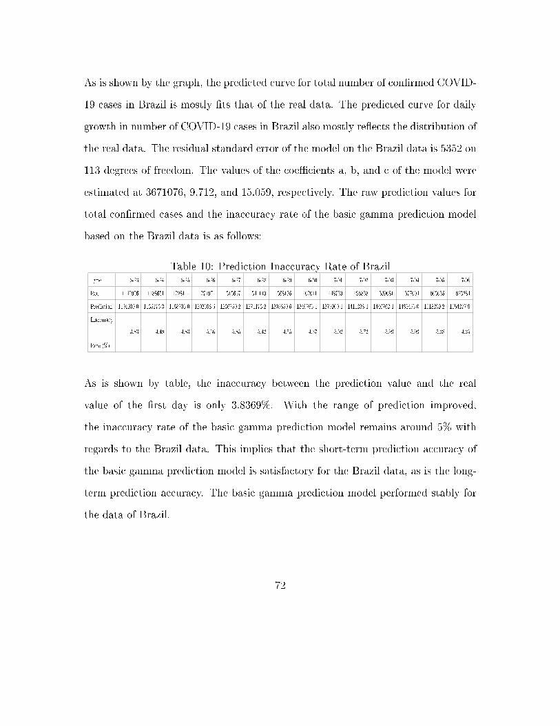
As is shown by the graph, the predicted curve for total number of con�rmed COVID-
19 cases in Brazil is mostly �ts that of the real data. The predicted curve for daily
growth in number of COVID-19 cases in Brazil also mostly re�ects the distribution of
the real data. The residual standard error of the model on the Brazil data is 5352 on
113 degrees of freedom. The values of the coe�cients a, b, and c of the model were
estimated at 3671076, 9.712, and 15.059, respectively. The raw prediction values for
total con�rmed cases and the inaccuracy rate of the basic gamma prediction model
based on the Brazil data is as follows:
Table 10: Prediction Inaccuracy Rate of BrazilType 6-23 6-24 6-25 6-26 6-27 6-28 6-29 6-30 7-01 7-02 7-03 7-04 7-05 7-06
Real 1145906 1188631 1228114 1274974 1313667 1344143 1368195 1402041 1448753 1496858 1539081 1577004 1603055 1623284
Prediction 1101939.0 1135176.3 1168735.0 1202598.5 1236750.2 1271173.2 1305850.6 1340765.4 1375900.4 1411238.4 1446762.4 1482455.0 1518299.2 1554277.9
Inaccuracy
Rate (%)
3.83 4.49 4.83 5.66 5.85 5.42 4.55 4.37 5.02 5.72 5.99 5.99 5.28 4.25
As is shown by table, the inaccuracy between the prediction value and the real
value of the �rst day is only 3.8369%. With the range of prediction improved,
the inaccuracy rate of the basic gamma prediction model remains around 5% with
regards to the Brazil data. This implies that the short-term prediction accuracy of
the basic gamma prediction model is satisfactory for the Brazil data, as is the long-
term prediction accuracy. The basic gamma prediction model performed stably for
the data of Brazil.
72
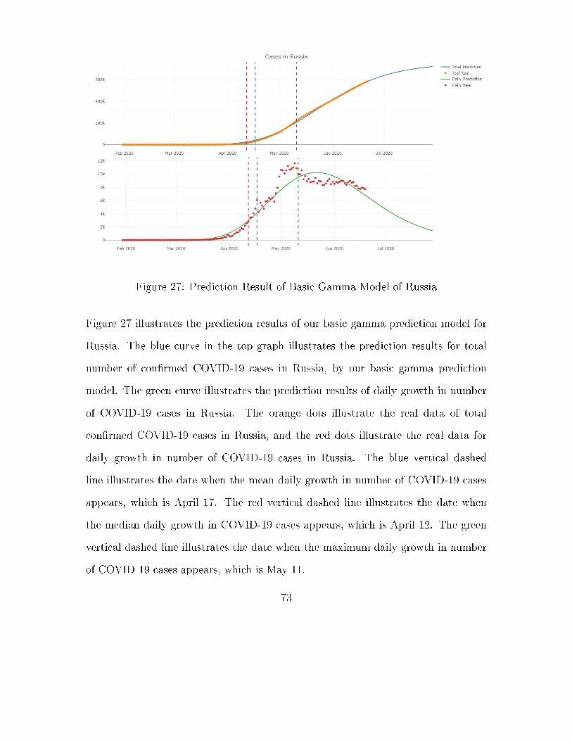
Figure 27: Prediction Result of Basic Gamma Model of Russia
Figure 27 illustrates the prediction results of our basic gamma prediction model for
Russia. The blue curve in the top graph illustrates the prediction results for total
number of con�rmed COVID-19 cases in Russia, by our basic gamma prediction
model. The green curve illustrates the prediction results of daily growth in number
of COVID-19 cases in Russia. The orange dots illustrate the real data of total
con�rmed COVID-19 cases in Russia, and the red dots illustrate the real data for
daily growth in number of COVID-19 cases in Russia. The blue vertical dashed
line illustrates the date when the mean daily growth in number of COVID-19 cases
appears, which is April 17. The red vertical dashed line illustrates the date when
the median daily growth in COVID-19 cases appears, which is April 12. The green
vertical dashed line illustrates the date when the maximum daily growth in number
of COVID-19 cases appears, which is May 11.
73

As is shown by graph, the predicted curve for total number of con�rmed COVID-19
case in Russia mostly �ts the distribution of the real data. The predicted curve
for daily growth in number of COVID-19 cases in Russia also mostly re�ects the
distribution of the real data. The residual standard error for model on the Russian
data is 826.6 on 139 degrees of freedom. The values of the coe�cients a, b, and c
of the model were estimated at 745054.4, 16.262, and 7.381, respectively. The raw
prediction values for total number of con�rmed cases, and the inaccuracy rate of the
basic gamma prediction model based on the Russia data, is as follows:
Table 11: Prediction Inaccuracy Rate of RussiaType 6-23 6-24 6-25 6-26 6-27 6-28 6-29 6-30 7-01 7-02 7-03 7-04 7-05 7-06
Real 598878 606043 613148 619936 626779 633563 640246 646929 653479 660231 666941 673564 680283 686852
Prediction 608642.4 615846.8 622893.3 629781.1 636509.9 643079.5 649490.0 655741.6 661834.9 667770.6 673549.6 679173.1 684642.2 689958.4
Inaccuracy
Rate (%)
1.63 1.61 1.58 1.58 1.55 1.50 1.44 1.36 1.27 1.14 0.99 0.83 0.64 0.45
As is shown by the table, the inaccuracy between the prediction value and the real
value of the �rst day is only 1.6304%. With the range of prediction improved, the
inaccuracy rate of the basic gamma prediction model stays around 1% with regards
to the Russian data. This implies that the short-term prediction accuracy of the
basic gamma prediction model is satisfactory on the Russia data of Russia, and
the long-term prediction accuracy performed very well. Overall, the basic gamma
prediction model performed stably for the data from Russia.
74

Figure 28: Prediction Result of Basic Gamma Model of India
Figure 28 illustrates the prediction results for our basic gamma prediction model in
India. The blue curve on the top graph illustrates the prediction results for total
number of con�rmed COVID-19 cases in India, by our basic gamma prediction model,
and the green curve illustrates the prediction results for daily growth in number of
COVID-19 cases in India. The orange dots illustrate the real data distribution for
total con�rmed COVID-19 cases in India, and the red dots illustrate the real data for
daily growth in number of cases. The blue vertical dashed line illustrates the date
when the mean daily growth in numbers of COVID-19 cases appears, which is May
5. The red vertical dashed line illustrates the date when the median daily growth in
number of COVID-19 cases appears, which is April 11. The green vertical dashed
line illustrates the date when the maximum daily growth in number of COVID-19
cases appears, which is June 20.
75

As is shown by graph, the predicted curve for total number of con�rmed COVID-19
case in India �ts that of the real data in India. The predicted curve for daily growth
in number of COVID-19 cases in India also basically re�ects the distribution of the
real data. The residual standard error of the model on the data from India is 433.3 on
140 degrees of freedom. The values of the coe�cients a, b, and c of the model were
estimated at 1247920, 8.018, and 39.175, respectively. The raw prediction values
for total number of con�rmed cases, and the inaccuracy rate of the basic gamma
prediction model for the India data, is as follows:
Table 12: Prediction Inaccuracy Rate of IndiaType 6-23 6-24 6-25 6-26 6-27 6-28 6-29 6-30 7-01 7-02 7-03 7-04 7-05 7-06
Real 456183 473105 490401 508953 528859 548318 566840 585481 604641 625544 648315 673165 697413 719664
Prediction 418935.2 433429.9 448259.9 463428.1 478937 494789.2 510987.1 527533.2 544429.5 561678.3 579281.6 597241.4 615559.4 634237.5
Inaccuracy
Rate (%)
8.16 8.38 8.59 8.94 9.43 9.76 9.85 9.89 9.95 10.20 10.64 11.27 11.73 11.87
As is shown by table, the inaccuracy between the prediction value and the real
value for the �rst day is only 8.1651%. With the range of prediction improved, the
inaccuracy rate of the basic gamma prediction model increases to 11.8703% for this
data. Thus, the prediction results are unsatisfactory. This implies that our basic
gamma prediction model should be changed to improve the performance for the data
from India.
76

Figure 29: Prediction Result of Basic Gamma Model of UK
Figure 29 illustrates the prediction results of our basic gamma prediction model for
the United Kingdom. The blue curve of the top graph illustrates the prediction
results for total number of con�rmed COVID-19 cases in the United Kingdom by
our gamma prediction model. The green curve illustrates the prediction results for
daily growth in number of COVID-19 cases in the United Kingdom. The orange dots
illustrate the real data for total con�rmed COVID-19 cases in the United Kingdom,
while the red dots illustrate the real data for daily growth in number of cases. The
blue vertical dashed line illustrates the date when the mean daily growth in number of
COVID-19 cases appears, which is March 26. The red vertical dashed line illustrates
the date when the median daily growth in number of COVID-19 cases appears, which
is June 1. The green vertical dashed line illustrates the date when the maximum
daily growth in COVID-19 cases appears, which is April 10.
77

As is shown by graph, the predicted curve for total number of con�rmed COVID-19
cases in the United Kingdom generally �ts the distribution of the real data for the
United Kingdom. The predicted curve for daily growth in number of COVID-19 cases
in the United Kingdom also basically re�ects the distribution of the real data. The
residual standard error of the model on the data from the United Kingdom is 703.5
on 139 degrees of freedom. The values of the coe�cients a, b, and c of the model were
estimated at 312342.6, 13.64, and 6.541, respectively. The raw prediction values for
total con�rmed cases and the inaccuracy rate of the basic gamma prediction model
based on the United Kingdom data is as follows:
Table 13: Prediction Inaccuracy Rate of The United KingdomType 6-23 6-24 6-25 6-26 6-27 6-28 6-29 6-30 7-01 7-02 7-03 7-04 7-05 7-06
Real 279566 280340 281037 281675 282308 282703 283307 283710 283770 283774 284276 284900 285416 285768
Prediction 279849.4 280195.3 280518.8 280821.2 281103.7 281367.5 281613.7 281843.3 282057.4 282257.0 282442.8 282615.8 282776.8 282926.5
Inaccuracy
Rate (%)
0.10 0.05 0.18 0.30 0.42 0.47 0.59 0.65 0.60 0.53 0.64 0.80 0.92 0.99
As is shown by table, the inaccuracy between the prediction value and the real value
for the �rst day is only 0.1014%. With the range of prediction improved, the inac-
curacy rate of the basic gamma prediction model increases to 0.9943% with regards
to the United Kingdom data. The inaccuracy remains below 1% for fourteen days
which implies that the short-term prediction accuracy, and the long-term prediction
accuracy of the basic gamma prediction model are both satisfactory using the United
Kingdom data.
78

Figure 30: Prediction Result of Basic Gamma Model of Peru
Figure 30 illustrates the prediction results of our basic gamma prediction model for
Peru. The blue curve of the top graph illustrates the prediction results for total
number of con�rmed COVID-19 cases in Peru, and the green curve illustrates the
prediction results for daily growth in number of COVID-19 cases in Peru. The orange
dots illustrate the real data for the total number of con�rmed COVID-19 cases in
Peru, and the red dots illustrate the real data for daily growth in number of COVID-
19 cases. The blue vertical dashed line illustrates the date when the mean daily
growth in number of COVID-19 cases appears, which is May 10. The red vertical
dashed line illustrates the date when the median daily growth in COVID-19 cases
appears, which is May 11. The green vertical dashed line illustrates the date when
the maximum daily growth in number of COVID-19 cases appears, which is June 14.
79

As is shown by graph, the predicted curve for total number of con�rmed COVID-19
cases in Peru generally �ts the distribution of the real data for Peru. The predicted
curve for daily growth in number of COVID-19 cases in Peru also re�ects the dis-
tribution of the real data. The residual standard error of the model on the data
for Peru is 1356 on 104 degrees of freedom. The values of the coe�cients a, b, and
c of the model were estimated at 352777, 9.7, and 9.8, respectively. The raw pre-
diction values for total con�rmed cases and the inaccuracy rate of the basic gamma
prediction model based on the Peru data is as follows:
Table 14: Prediction Inaccuracy Rate of PeruType 6-23 6-24 6-25 6-26 6-27 6-28 6-29 6-30 7-01 7-02 7-03 7-04 7-05 7-06
Real 260810 264689 268602 272364 275989 279419 282365 285213 288477 292004 295599 299080 302718 305703
Prediction 252829.0 256735.9 260573.3 264340.0 268035.1 271657.6 275207.0 278682.6 282084.0 285410.9 288663.2 291840.7 294943.5 297971.8
Inaccuracy
Rate (%)
3.06 3.00 2.98 2.94 2.88 2.77 2.53 2.28 2.21 2.25 2.34 2.42 2.56 2.52
As is shown by table, the inaccuracy between the prediction value and the real
value for the �rst day is only 3.0601%. With the range of prediction improved,
the inaccuracy rate of the basic gamma prediction model decreases to 2.529% with
regards to the Peru data. The overall inaccuracy remains below 3.1% for fourteen
days of prediction. This implies that the short-term prediction accuracy of the
basic gamma prediction model is satisfactory for Peru, and the long-term prediction
accuracy also performed well.
80

Figure 31: Prediction Result of Basic Gamma Model of Spain
Figure 31 illustrates the prediction results of our basic gamma prediction model for
Spain. The blue curve on the top graph illustrates the prediction results for total
number of con�rmed COVID-19 cases in Spain by basic gamma prediction model.
The green curve illustrates the prediction results for Spain's daily growth in number
of COVID-19 cases. The orange dots illustrate the real data for total con�rmed
COVID-19 cases in Spain, and the red dots illustrate the real data for daily growth
in number of COVID-19 cases. The blue vertical dashed line illustrates the date
when the mean daily growth in COVID-19 cases appears, which is April 26. The red
vertical dashed line illustrates the date when the median daily growth in COVID-19
cases appears, which is May 4. The green vertical dashed line illustrates the date
when the maximum daily growth in COVID-19 cases appears, which is March 25.
81

As is shown by graph, the predicted curve for the total number of con�rmed COVID-
19 cases in Spain generally �ts the distribution of the real data. The predicted curve
for daily growth in number of COVID-19 cases in Spain also generally re�ects the
distribution of the real data. The residual standard error of the model on the data
from Spain is 1418 on 138 degrees of freedom. The values of the coe�cients a, b,
and c of the model were estimated at 222835.5, 26.671, and 2.375, respectively. The
raw prediction values for total con�rmed cases, and the inaccuracy rate of the basic
gamma prediction model based on the Spain data, is as follows:
Table 15: Prediction Inaccuracy Rate of SpainType 6-23 6-24 6-25 6-26 6-27 6-28 6-29 6-30 7-01 7-02 7-03 7-04 7-05 7-06
Real 246752 247086 247486 247905 248469 248770 248970 249271 249659 250103 250545 250545 250545 251789
Prediction 222835.6 222835.6 222835.6 222835.6 222835.7 222835.7 222835.7 222835.7 222835.7 222835.7 222835.7 222835.7 222835.7 222835.7
Inaccuracy
Rate (%)
9.69 9.81 9.96 10.11 10.31 10.42 10.49 10.60 10.74 10.90 11.05 11.05 11.05 11.49
As is shown by table, the inaccuracy between the prediction value and the real value
for the �rst day is 9.6925%. With the range of prediction improved, the inaccuracy
rate of the basic gamma prediction model increases to 11.499% with regards to the
data from Spain. The inaccuracy stays around 10% for 14 days of predictions. This
implies that both the short-term prediction accuracy and the long-term prediction
accuracy of the basic gamma prediction model is not very good for the data from
Spain. However, the performance of the model stays stable, so we can manually
estimate the error and correct it.
82

Figure 32: Prediction Result of Basic Gamma Model of Chile
Figure 32 illustrates the prediction results of our basic gamma prediction model for
Chile. The blue curve on the top graph illustrates the prediction results for the
total number of con�rmed COVID-19 cases in Chile, by our basic gamma prediction
model. The green curve illustrates the prediction results for daily growth in number
COVID-19 cases in Chile. The orange dots illustrate the distribution of the real
data for total con�rmed COVID-19 cases in Chile, and the red dots illustrate the
real data for daily growth in number of COVID-19 cases. The blue vertical dashed
line illustrates the date when the mean daily growth in number of COVID-19 cases
appears, which is May 18. The red vertical dashed line illustrates the date when the
median daily growth in number of COVID-19 cases appears, which is April 28. The
green vertical dashed line illustrates the date when the maximum daily growth in
number of COVID-19 cases appears, which is June 17.
83

As is shown by graph, the predicted curve for the total number of con�rmed COVID-
19 case in Chile generally �ts the distribution of the real data. The predicted curve
for daily growth in number of COVID-19 cases in Chile also generally re�ects the
distribution of the real data. The residual standard error of the model for the data
from Chile is 2855 on 107 degrees of freedom. The values of the coe�cients a, b,
and c of the model were estimated at 423589400, 5.02, and 169.9, respectively. The
raw prediction values for total con�rmed cases and the inaccuracy rate of the basic
gamma prediction model based on the data from Chile is as follows:
Table 16: Prediction Inaccuracy Rate of ChileType 6-23 6-24 6-25 6-26 6-27 6-28 6-29 6-30 7-01 7-02 7-03 7-04 7-05 7-06
Real 250767 254416 259064 263360 267766 271982 275999 279393 282043 284541 288089 291847 295532 298557
Prediction 211682.9 217440.1 223050.7 228507.1 233802.7 238932.3 243891.2 248675.9 253283.8 257713.2 261963.3 266034.0 269925.9 273640.5
Inaccuracy
Rate (%)
15.58 14.53 13.90 13.23 12.68 12.15 11.63 10.99 10.19 9.42 9.06 8.84 8.66 8.34
As is shown by table, the inaccuracy between the prediction value and the real value
for the �rst day is 15.5858%. With the range of prediction improved, the inaccuracy
rate of the basic gamma prediction model decreases to 8.3456%. This implies that the
prediction accuracy of the basic gamma model increases as the range in prediction
improves for the data from Chile.
84

Figure 33: Prediction Result of Basic Gamma Model of Italy
Figure 33 illustrates the prediction results of our basic gamma prediciton model for
Italy. The blue curve of the top graph illustrates the prediction results for the total
number of con�rmed COVID-19 cases in Italy, by our basic gamma prediction model.
The green curve illustrates the prediction results for the daily growth in number of
COVID-19 cases in Italy. The orange dots illustrate the distribution of the real data
for total con�rmed number of COVID-19 cases in Italy, and the red dots illustrate the
real data for daily growth in number of COVID-19 cases. The blue vertical dashed
line illustrates the date when the mean daily growth in number of COVID-19 cases
appears, which is April 27. The red vertical dashed line illustrates the date when
the median daily growth in number of COVID-19 cases appears, which is May 15.
The green vertical dashed line illustrates the date when the maximum daily growth
in COVID-19 cases appears, which is March 21.
85

As is shown by graph, the predicted curve for total number of con�rmed COVID-19
cases in Italy generally �ts the distribution of the real data. The predicted curve
for daily growth in number of COVID-19 cases in Italy also generally re�ects the
distribution of the real data. The residual standard error of the model for the data
from Italy is 429.5 on 139 degrees of freedom. The values of the coe�cients a, b, and
c of the model were estimated at 232799.6, 11.899, and 5.487, respectively. The raw
prediction values for the total number of con�rmed cases, and the inaccuracy rate of
the basic gamma prediction model for the Italy data, is as follows:
Table 17: Prediction Inaccuracy Rate of ItalyType 6-23 6-24 6-25 6-26 6-27 6-28 6-29 6-30 7-01 7-02 7-03 7-04 7-05 7-06
Real 238833 239410 239706 239961 240136 240310 240436 240578 240760 240961 241184 241419 241611 241819
Prediction 232771.0 232786.3 232800.0 232812.3 232823.3 232833.2 232842.1 232850.1 232857.2 232863.6 232869.3 232874.4 232879.0 232883.1
Inaccuracy
Rate (%)
2.53 2.76 2.88 2.97 3.04 3.11 3.15 3.21 3.28 3.36 3.44 3.53 3.61 3.69
As is shown by table, the inaccuracy between the prediction value and the real
value for the �rst day is only 2.5382%. With the range of prediction improved,
the inaccuracy rate of the basic gamma prediction model increases to 3.6953% with
regards to the data from Italy. Even though the inaccuracy increases slightly, the
overall accuracy of the basic gamma prediction model performs well in the short-term
and the long-term based on the data from Italy.
Lastly, we evaluated our application gamma prediction model for the data from Iran,
the prediction curve for which is shown below:
86

Figure 34: Prediction Result of Application Gamma for Iran
Figure 34 illustrates the prediction results of our application gamma prediction model
for Iran. The blue curve on the top graph illustrates the prediction results for
the total number of con�rmed COVID-19 cases in Iran, by our application gamma
prediction model. The green curve illustrates the prediction results for daily growth
in number COVID-19 cases in Iran. The orange dots illustrate the distribution of the
real data for total con�rmed COVID-19 cases in Iran, and the red dots illustrate the
real data for daily growth in number of COVID-19 cases. The blue vertical dashed
line illustrates the date when the mean daily growth in number of COVID-19 cases
appears, which is March 15. The red vertical dashed line illustrates the date when
the median daily growth in number of COVID-19 cases appears, which is April 20.
The green vertical dashed line illustrates the date when the maximum daily growth
in number of COVID-19 cases appears, which is June 5.
87

As is shown by graph, the predicted curve for total number of con�rmed COVID-19
cases in Iran generally �ts the distribution of the real data for Iran. The predicted
curve for daily growth in number of COVID-19 cases in Iran also generally re�ects
the trend of the real data. The residual standard error of the model for the data
from Iran is 352.3 on 147 degrees of freedom. The values of the coe�cients a, b, c, d,
and e of the model were estimated at 230971.042, 59.748, 2.314, 14.011, and 5.514,
respectively. The raw prediction values for total con�rmed cases and the inaccuracy
rate of the application gamma prediction model based on the data for Iran is as
follows:
Table 18: Prediction Inaccuracy Rate of IranType 6-23 6-24 6-25 6-26 6-27 6-28 6-29 6-30 7-01 7-02 7-03 7-04 7-05 7-06
Real 209970 212501 215096 217724 220180 222669 225205 227662 230211 232863 235429 237878 240438 243051
Prediction 206784.9 208494 210119.9 211662.8 213123.5 214503 215802.9 217024.8 218170.8 219243.2 220244.5 221177.2 222044.2 222848.4
Inaccuracy
Rate (%)
1.51 1.88 2.31 2.78 3.20 3.66 4.17 4.67 5.23 5.84 6.44 7.02 7.65 8.31
As is shown by table, the inaccuracy between the prediction value and the real value
for the �rst day is only 1.5169%. With the range of prediction improved, the inac-
curacy rate of the basic gamma prediction model increases to 8.3121% with regards
to the Iran data. However, the inaccuracy stays below 5% until the eight day. This
implies that the short-term prediction accuracy of the application gamma prediction
model is satisfactory using the data from Iran, and the long-term prediction accu-
racy of the model is also basically acceptable. Therefore, the application gamma
prediction model is an e�ective forecasting tool for data that is not similar to the
88

standard gamma distribution.
According to our evaluation of the performance of our prediction models, using the
data from the 10 countries with the highest number of total con�rmed COVID-19
cases as of June 22, we made some conclusions. First, the predicted curves for the
total number of con�rmed COVID-19 cases produced by our models, generally �ts
the distributions of the real data from the ten countries. Second, the predicted
curves for the daily growth in number of COVID-19 cases produced by our models
also basically re�ects the trends shown by the real data from the di�erent countries.
Third, the prediction model generally has high accuracy for short-term predictions,
while its accuracy for long-term predictions depend more on the distribution of the
real data. Fourth, the performance of the application gamma prediction model on
the data from Iran showed signi�cant improvement from the basic gamma prediction
model using the same data. To further verify the predictive e�ect of our model using
data from other countries, we calculated the inaccuracies of our prediction models
using the data from the 19 countries with the highest number of total con�rmed
COVID-19 cases as of June 22. The results are as follows:
89

Table 19: Prediction Inaccuracy Rate of Top 19 CountriesCountry Type 2020-06-23 2020-06-24 2020-06-25 2020-06-26 2020-06-27 2020-06-28 2020-06-29 2020-06-30 2020-07-01 2020-07-02 2020-07-03 2020-07-04 2020-07-05 2020-07-06
Real 2347491.00 2382426.00 2422299.00 2467554.00 2510259.00 2549294.00 2590668.00 2636414.00 2687588.00 2742049.00 2795361.00 2841241.00 2891124.00 2936077.00
Prediction 2323456.00 2338671.00 2353538.00 2368058.00 2382237.00 2396078.00 2409585.00 2422763.00 2435616.00 2448147.00 2460363.00 2472268.00 2483865.00 2495162.00US
Inaccuracy Rate (%) 1.02 1.84 2.84 4.03 5.10 6.01 6.99 8.10 9.38 10.72 11.98 12.99 14.09 15.02
Real 1145906.00 1188631.00 1228114.00 1274974.00 1313667.00 1344143.00 1368195.00 1402041.00 1448753.00 1496858.00 1539081.00 1577004.00 1603055.00 1623284.00
Prediction 1101939.05 1135176.34 1168734.99 1202598.49 1236750.18 1271173.20 1305850.62 1340765.39 1375900.38 1411238.44 1446762.38 1482455.02 1518299.22 1554277.88Brazil
Inaccuracy Rate (%) 3.84 4.50 4.83 5.68 5.86 5.43 4.56 4.37 5.03 5.72 6.00 6.00 5.29 4.25
Real 598878.00 606043.00 613148.00 619936.00 626779.00 633563.00 640246.00 646929.00 653479.00 660231.00 666941.00 673564.00 680283.00 686852.00
Prediction 608642.40 615846.81 622893.28 629781.13 636509.94 643079.54 649490.00 655741.63 661834.93 667770.63 673549.65 679173.08 684642.20 689958.44Russia
Inaccuracy Rate (%) 1.63 1.62 1.59 1.59 1.55 1.50 1.44 1.36 1.28 1.14 0.99 0.83 0.64 0.45
Real 456183.00 473105.00 490401.00 508953.00 528859.00 548318.00 566840.00 585481.00 604641.00 625544.00 648315.00 673165.00 697413.00 719664.00
Prediction 418935.20 433429.90 448259.90 463428.10 478937.00 494789.20 510987.10 527533.20 544429.50 561678.30 579281.60 597241.40 615559.40 634237.50India
Inaccuracy Rate (%) 8.17 8.39 8.59 8.94 9.44 9.76 9.85 9.90 9.96 10.21 10.65 11.28 11.74 11.87
Real 279566.00 280340.00 281037.00 281675.00 282308.00 282703.00 283307.00 283710.00 283770.00 283774.00 284276.00 284900.00 285416.00 285768.00
Prediction 279849.43 280195.31 280518.80 280821.18 281103.68 281367.47 281613.67 281843.32 282057.43 282256.96 282442.80 282615.81 282776.79 282926.52United Kingdom
Inaccuracy Rate (%) 0.10 0.05 0.18 0.30 0.43 0.47 0.60 0.66 0.60 0.53 0.64 0.80 0.92 0.99
Real 260810.00 264689.00 268602.00 272364.00 275989.00 279419.00 282365.00 285213.00 288477.00 292004.00 295599.00 299080.00 302718.00 305703.00
Prediction 252829.01 256735.94 260573.34 264340.05 268035.10 271657.64 275206.99 278682.58 282083.99 285410.90 288663.15 291840.67 294943.50 297971.80Peru
Inaccuracy Rate (%) 3.06 3.00 2.99 2.95 2.88 2.78 2.54 2.29 2.22 2.26 2.35 2.42 2.57 2.53
Real 246752.00 247086.00 247486.00 247905.00 248469.00 248770.00 248970.00 249271.00 249659.00 250103.00 250545.00 250545.00 250545.00 251789.00
Prediction 222835.59 222835.61 222835.63 222835.64 222835.65 222835.66 222835.66 222835.67 222835.67 222835.68 222835.68 222835.68 222835.68 222835.68Spain
Inaccuracy Rate (%) 9.69 9.81 9.96 10.11 10.32 10.43 10.50 10.61 10.74 10.90 11.06 11.06 11.06 11.50
Real 250767.00 254416.00 259064.00 263360.00 267766.00 271982.00 275999.00 279393.00 282043.00 284541.00 288089.00 291847.00 295532.00 298557.00
Prediction 211682.94 217440.14 223050.69 228507.06 233802.75 238932.28 243891.17 248675.87 253283.80 257713.23 261963.32 266033.99 269925.93 273640.52Chile
Inaccuracy Rate (%) 15.59 14.53 13.90 13.23 12.68 12.15 11.63 10.99 10.20 9.43 9.07 8.84 8.66 8.35
Real 238833.00 239410.00 239706.00 239961.00 240136.00 240310.00 240436.00 240578.00 240760.00 240961.00 241184.00 241419.00 241611.00 241819.00
Prediction 232771.05 232786.28 232799.97 232812.27 232823.31 232833.21 232842.09 232850.05 232857.19 232863.57 232869.29 232874.41 232878.98 232883.07Italy
Inaccuracy Rate (%) 2.54 2.77 2.88 2.98 3.05 3.11 3.16 3.21 3.28 3.36 3.45 3.54 3.61 3.70
Real 209970.00 212501.00 215096.00 217724.00 220180.00 222669.00 225205.00 227662.00 230211.00 232863.00 235429.00 237878.00 240438.00 243051.00
Prediction 206784.90 208494.00 210119.90 211662.80 213123.50 214503.00 215802.90 217024.80 218170.80 219243.20 220244.50 221177.20 222044.20 222848.40Iran
Inaccuracy Rate (%) 1.52 1.89 2.31 2.78 3.20 3.67 4.17 4.67 5.23 5.85 6.45 7.02 7.65 8.31
Real 192452.00 192265.00 192010.00 193346.00 193152.00 192429.00 194109.00 194373.00 194985.00 195458.00 195904.00 195546.00 195535.00 196748.00
Prediction 172949.87 172949.89 172949.91 172949.93 172949.94 172949.94 172949.95 172949.95 172949.96 172949.96 172949.96 172949.96 172949.97 172949.97France
Inaccuracy Rate (%) 10.13 10.05 9.93 10.55 10.46 10.12 10.90 11.02 11.30 11.52 11.72 11.56 11.55 12.10
Real 192480.00 192871.00 193371.00 194036.00 194458.00 194693.00 195042.00 195418.00 195893.00 196370.00 196780.00 197198.00 197523.00 198064.00
Prediction 169215.89 169215.91 169215.93 169215.94 169215.96 169215.97 169215.97 169215.98 169215.98 169215.99 169215.99 169215.99 169215.99 169216.00Germany
Inaccuracy Rate (%) 12.09 12.26 12.49 12.79 12.98 13.09 13.24 13.41 13.62 13.83 14.01 14.19 14.33 14.56
Real 190165.00 191657.00 193115.00 194511.00 195883.00 197239.00 198613.00 199906.00 201098.00 202284.00 203456.00 204610.00 205758.00 206844.00
Prediction 185347.02 185582.54 185804.36 186013.23 186209.85 186394.88 186568.96 186732.69 186886.65 187031.37 187167.39 187295.19 187415.23 187527.97Turkey
Inaccuracy Rate (%) 2.53 3.17 3.79 4.37 4.94 5.50 6.06 6.59 7.07 7.54 8.01 8.46 8.91 9.34
Real 188926.00 192970.00 195745.00 198883.00 202955.00 206512.00 209337.00 213470.00 217809.00 221896.00 221896.00 225283.00 231818.00 234509.00
Prediction 155805.28 160424.21 164965.04 169420.81 173785.14 178052.24 182216.91 186274.55 190221.15 194053.29 197768.13 201363.39 204837.33 208188.73Pakistan
Inaccuracy Rate (%) 17.53 16.87 15.72 14.81 14.37 13.78 12.96 12.74 12.67 12.55 10.87 10.62 11.64 11.22
Real 191410.00 196847.00 202951.00 208392.00 212802.00 216852.00 220657.00 226089.00 231770.00 238511.00 245251.00 252165.00 256848.00 261750.00
Prediction 182437.07 187488.10 192600.65 197773.65 203006.00 208296.55 213644.16 219047.66 224505.85 230017.53 235581.45 241196.38 246861.05 252574.18Mexico
Inaccuracy Rate (%) 4.69 4.75 5.10 5.10 4.60 3.95 3.18 3.11 3.13 3.56 3.94 4.35 3.89 3.51
Real 119198.00 122660.00 126606.00 130474.00 133978.00 137787.00 141801.00 145483.00 149258.00 153277.00 156391.00 159679.00 162417.00 165618.00
Prediction 110477.75 113985.89 117514.77 121061.63 124623.75 128198.39 131782.86 135374.48 138970.61 142568.64 146165.99 149760.16 153348.66 156929.08Bangladesh
Inaccuracy Rate (%) 7.32 7.07 7.18 7.21 6.98 6.96 7.06 6.95 6.89 6.99 6.54 6.21 5.58 5.25
Real 103767.00 104087.00 104463.00 104629.00 104878.00 105193.00 105830.00 106097.00 106288.00 106643.00 106962.00 107185.00 107394.00 107815.00
Prediction 105327.03 105589.90 105838.66 106073.93 106296.33 106506.43 106704.82 106892.04 107068.64 107235.12 107391.99 107539.73 107678.79 107809.63Canada
Inaccuracy Rate (%) 1.50 1.44 1.32 1.38 1.35 1.25 0.83 0.75 0.73 0.56 0.40 0.33 0.27 0.00
Real 89579.00 90778.00 91838.00 92784.00 93663.00 94413.00 95106.00 96088.00 97003.00 97897.00 98653.00 99183.00 99799.00 100345.00
Prediction 85119.89 86222.26 87290.40 88324.46 89324.62 90291.15 91224.39 92124.72 92992.58 93828.46 94632.88 95406.43 96149.70 96863.34Qatar
Inaccuracy Rate (%) 4.98 5.02 4.95 4.81 4.63 4.37 4.08 4.12 4.13 4.16 4.08 3.81 3.66 3.47
Real 84653.00 84673.00 84701.00 84725.00 84743.00 84757.00 84780.00 84785.00 84816.00 84830.00 84838.00 84857.00 84871.00 84889.00
Prediction 81146.16 81146.16 81146.16 81146.16 81146.16 81146.16 81146.16 81146.16 81146.16 81146.16 81146.16 81146.16 81146.16 81146.16China
Inaccuracy Rate (%) 4.14 4.17 4.20 4.22 4.24 4.26 4.29 4.29 4.33 4.34 4.35 4.37 4.39 4.41
90

According to the table, the inaccuracy of our prediction models for the �rst day were
over 10% based on using the data from the following four countries: Chile, France,
Germany, and Pakistan. For the other fourteen countries, the inaccuracies of the
�rst-day predictions were all lower than 10%. In these fourteen countries, there were
twelve countries for which the inaccuracies of the model were lower than 5% for the
�rst-day prediction. Furthermore, with countries for which the model predicted with
an inaccuracy rate lower than 5% for the �rst day, the inaccuracy rate for the other
thirteen days mostly remained below 5%. These results imply that, if the prediction
model performs well using the data from the �rst-day of a given country, it will
probably continue to perform well for the following thirteen days.
91

5 COVID-19 Pandemic Forecasting Web Page
We developed a web page designed to provide the following information to users:
the graph of real daily growth in con�rmed COVID-19 cases, the graph of real total
con�rmed COVID-19 cases, the graph of predicted daily growth in con�rmed cases,
the graph of predicted total con�rmed cases, and the corresponding predicted data
over 14 days for the 19 countries with the highest number of con�rmed cases. Since
all of the data processing and analysis in this thesis are implemented by R, and
the data visualization is implemented by the R library Plotly, a framework that is
integrated with the R library Plotly would be optimal for the information presented
in this thesis. Thus, we chose the Dash as the framework to build our web page.
Dash for R is an open-source framework for building analytical applications, with no
javascript required, and it is tightly integrated with the Plotly graphing library [44].
Dash is a productive framework for building web applications in both R and Python.
Written on top of Fiery/Flask, Plotly.js, and React.js, Dash is ideal for building data
visualization apps with highly customizable user interfaces in pure R or Python. It's
especially well-suited for anyone who works with data. Through a couple of simple
patterns, Dash simpli�es all of the technologies and protocols that are required to
build an interactive web-based application. Dash apps are rendered in the web
browser, and the developer can deploy apps to servers and then share them through
URLs. Since Dash apps are viewed in web browsers, Dash is inherently across-
platforms and is mobile ready.
92

Our COVID-19 pandemic forecasting web page is now online at [45]. The COVID-19
forecasting web page is composed of two subpages. The front end of the home page
is shown below:
Figure 35: Front End of the Home Page
The home page of the COVID-19 pandemic forecasting web page is mainly composed
of �ve divisions, two buttons, and one drop-down box. The upper left division was
developed to summarize the information from the model trained by the data of the
selected country. The middle division on the left side was developed to illustrate
93

the total number of con�rmed COVID-19 cases for the selected country as of June
22. The bottom left division was developed to illustrate a list of the 19 countries
with the highest number of con�rmed cases as of June 22. The upper right division
was developed to display the data for the real total number of con�rmed COVID-19
cases in the selected country as of 22 June, as well as the predicted curve for the
total number of con�rmed COVID-19 cases generated by the prediction model of this
thesis. The bottom right division was developed to display the data for the real daily
growth in number of COVID-19 cases in the selected country as of June 22, as well
as the predicted curve for the daily growth in cases as generated by the prediction
model of this thesis. The drop-down box at the top was designed for selecting which
country's data is to be displayed. The second button on the top was developed to
jump to the second subpage of the COVID-19 pandemic forecasting website. The
front end of the second sub-page is shown below:
94

Figure 36: Front End of the Predict Page
The prediction page was developed to display the table showing the raw prediction
values for the following 14 days. This shows the predictions for the total number of
con�rmed COVID-19 cases for the 19 aforementioned countries. Depending on the
country name selected by users, the content of the home page would update to re�ect
that country's data. The process used for the back end of the COVID-19 pandemic
forecasting web page is as follows:
95

Figure 37: Process of the Back End of the COVID-19 Pandemic Forecasting Web
Page
After users select a country, the name of the country will be sent to the back- end
96

program. The speci�c process for the data preprocessing is discussed in chapter 3.
Then, the back-end program decides which prediction model will be utilized to gen-
erate the prediction data. If the selected country is Iran, the back-end program will
choose the application gamma prediction model. If the selected country is not Iran,
the back-end program will choose the basic gamma prediction model. The speci�c
processes for the basic and application gamma prediction models, respectively, are
discussed in chapter 4. After the model has been trained to generate the prediction
values, the prediction value will be used to generate the prediction curves for total
con�rmed COVID-19 cases, and daily growth in COVID-19 cases, for the selected
countries.
The information provided by the COVID-19 pandemic forecasting web page can be
used by individuals as well as public organizations. Public organizations can use the
information to more e�ciently allocate medical resources, as well as establish policy
to prevent the spread of COVID-19. Individuals can use the information to help
them make decisions regarding their own life plan during the COVID-19 pandemic.
For example, whether or not to participate in or cancel large gatherings, whether to
wear a mask, and whether to reduce unnecessary travel.
97

6 Conclusion and Future Work
6.1 Conclusion
In this project, we built two prediction models to forecast the total number of con-
�rmed cases of COVID-19, and the daily growth in the number of cases of COVID-
19, for di�erent countries. COVID-19 is a highly contagious atypical pneumonia
attributed to a novel coronavirus. The global economy and people's lives have been
tremendously a�ected by COVID-19 pandemic. WHO made the announcement that
the event constitutes a Public Health Emergency of International Concern on Jan-
uary 30. The core of our prediction algorithms is composed of a gamma distribution
with shape K and scale θ as parameters. The model has two versions. The simpler
version is referred to as the basic gamma prediction model, and lower consumption
of computing power is implemented for prediction in most countries. The advanced
version is referred to as the application gamma prediction model, and a higher con-
sumption of computing power is implemented for the prediction of countries with
more complex data.
The data is extracted from the original data of the interactive web-based dash-
board developed by the Center for System Science and Engineering (CSSE) at Johns
Hopkins University, Baltimore, MD, USA. The corresponding data preprocessing
procedure used to construct the data for regression, and to construct the data for
visualization, has been introduced in the thesis. The basic analysis for the top 10
countries from the original data source has been performed in the thesis in order to
98

estimate the mathematical core of the prediction model.
The evaluation of the performance of the prediction models in this thesis has been
done using the data from the ten countries with the highest number of total con-
�rmed COVID-19 cases as of June 22. The predicted curves for the total number of
con�rmed COVID-19 cases produced by our models have been shown to generally �t
the real data for the di�erent countries. The predicted curves for the daily growth
in the number of COVID-19 cases produced by our models have also been shown to
generally re�ect the trends displayed by the real data for the di�erent countries. The
prediction model generally has a high level of accuracy for short-term predictions,
while the accuracy of its long-term predictions depends on the distribution of the
real data. The inaccuracies of our prediction models using the data from the 19
countries with the highest total number of con�rmed COVID-19 cases as of June 22
have been calculated. If the prediction model shows high accuracy after the �rst day
using data from a given country, it is like that it will continue performing well for
the following thirteen days.
A web page has been developed as a part of this thesis meant to provide information
to users. This included the graphs of the real daily growth in the number of con-
�rmed cases, the graphs showing the real total number of con�rmed cases, the graphs
showing our predictions for both of these values, and the corresponding predicted
data over 14 days for the 19 countries that have the high number of total con�rmed
cases. Dash for R, an open-source framework, has been chosen for the COVID-19
99

pandemic forecasting web page in this thesis.
6.2 Future Work
As for future work, it will be interesting to expand the prediction model for other
data metrics since we only used the total number of con�rmed cases and the daily
growth in the number of cases of COVID-19 in di�erent countries for this model. For
example, we could use the mortality and recovery rate data for the di�erent countries
as well. Furthermore, researching to learn how to decrease the inaccuracies of our
prediction models for some countries would be worthwhile. Since the data about
COVID-19 is going to increase only time, some prediction models could require
a large amount of data to train them. For example, deep learning will be worth
attempting in the future.
100

References
[1] Chan, J. F. et al. A familial cluster of pneumonia associated with the 2019 novel
coronavirus indicating person-to-person transmission: a study of a family clus-
ter. Lancet (London, England). https://doi.org/10.1016/s0140-6736 (20)30154-9
(2020).
[2] World Health Organization Pneumonia of unknown cause�China.
https://www.who.int/csr/don/05-january-2020-pneumonia-of-unkowncause-
china/en.
[3] WHO Novel Coronavirus(2019-nCoV) Situation Report�22.
https://www.who.int/csr/don/05-january-2020-pneumonia-of-unkowncause-
china/en.
[4] WHO Novel Coronavirus(2019-nCoV) Situation Report�22.
https://www.who.int/csr/don/05-january-2020-pneumonia-of-unkowncause-
china/en.
[5] Hui, D. S. et al. The continuing 2019-nCoV epidemic threat of novel coron-
aviruses to global health�the latest 2019 novel coronavirus outbreak in Wuhan,
China. Int. J. Infect. Dis. 91, 264�266 (2020).
[6] Chen, N. et al. Epidemiological and clinical characteristics of 99 cases of 2019
novel coronavirus pneumonia in Wuhan, China: a descriptive study. Lancet
https://doi.org/10.1016/S0140-6736(20)30211-7.
101

[7] Real-time big data report on the epidemic (in Chinese) 2020. Available on-
line at https://voice.baidu.com/act/newpneumonia/newpneumonia/?from=
osari_aladin_top1.
[8] Coronavirus disease 2019 (COVID-19) Situation Report�25 2020. Available
online at https://www.who.int/docs/default-source/coronaviruse/
situation-reports/20200214-sitrep-25-covid-19.pdf?sfvrsn=61dda7d_
2.
[9] Situation Updates - SARS: Update 95 - Chronology of a serial killer 2003. Avail-
able online at https://www.who.int/csr/don/2003_06_18/en/.
[10] WHO. Statement on the Second Meeting of the International Health Reg-
ulations (2005) Emergency Committee Regarding the Outbreak of Novel
Coronavirus (2019-nCoV) at https://www.who.int/news-room/detail/
30-01-2020-statementon-the-second-meeting).
[11] Sung Y. Park, Anil K. Bera, Maximum entropy autoregressive conditional het-
eroskedasticity model, Journal of Econometrics, Volume 150, Issue 2, 2009,
Pages 219-230, ISSN 0304-4076, https://doi.org/10.1016/j.jeconom.2008.
12.014.
[12] Hogg, R. V.; Craig, A. T. (1978). Introduction to Mathematical Statistics (4th
ed.). New York: Macmillan. pp. Remark 3.3.1. ISBN 0023557109.
[13] Seber, G. A. F.; Wild, C. J. (1989). Nonlinear Regression. New York: John
Wiley and Sons. ISBN 0471617601.
102

[14] Meade, N.; Islam, T. (1995). Prediction Intervals for Growth Curve Forecasts.
Journal of Forecasting. 14 (5): 413�430. doi:10.1002/for.3980140502.
[15] Bethea, R. M.; Duran, B. S.; Boullion, T. L. (1985). Statistical Methods for
Engineers and Scientists. New York: Marcel Dekker. ISBN 0-8247-7227-X.
[16] Kakiashvili T, Koczkodaj WW,Woodbury-Smith M. Improving the medical
scale predictability by the pairwise comparisons method: evidence from a clini-
cal data study. Comput Methods Programs Biomed 2012; 105:210�6.
[17] Paul G. Approaches to abductive reasoning: an overview. Arti�cial Intelligence
Review 1993; 7:109�52.
[18] Bai, Z., Gong, Y., Tian, X. et al. The Rapid Assessment and Early Warn-
ing Models for COVID-19. Virol. Sin. (2020). https://doi-org.librweb.
laurentian.ca/10.1007/s12250-020-00219-0.
[19] Wassenaar, T.M., Zou, Y.rapid classi�cation of beta coronaviruses and
identi�cation.https://doi.org/10.1111/lam.13285.
[20] Paraskevis D, Kostaki EG, Magiorkinis G, Panayiotakopoulos G,Sourvinos G,
Tsiodras S (2020) Full-genome evolutionary analysis of the novel corona virus
(2019-nCoV) rejects the hypothesis of emergence as a result of a recent recom-
bination event. Infect Genet Evol 79:104212
[21] Wong MC, Cregeen SJJ, Ajami NJ, Petrosino JF (2020) Evidence of recombi-
nation in coronaviruses implicating pangolin origins of nCoV-2019. bioRxiv.
103

[22] Zhao S, Musa SS, Lin Q, Ran J, Yang G, Wang W, Lou Y, Yang L, Gao D, He
D (2020) Estimating the unreported number of novel coronavirus (2019-nCoV)
cases in China in the �rst half of January 2020: a data-driven Modelling analysis
of the early outbreak. J Clin Med 9:388.
[23] Riou J, Althaus CL (2020) Pattern of early human-to-human transmission of
Wuhan 2019 novel coronavirus (2019-nCoV), December 2019 to January 2020.
Eurosurveillance 25:2000058.
[24] W.W. Koczkodaj, M.A. Mansournia, W. Pedrycz, A. Wolny-Dominiak, P.F.
Zabrodskii, D. Strzaªka, T. Armstrong, A.H. Zolfaghari, M. D¦bski, J. Mazurek,
1,000,000 cases of COVID-19 outside of China: The date predicted by a sim-
ple heuristic, Global Epidemiology, Volume 2, 2020, 100023, ISSN 2590-1133,
https://doi.org/10.1016/j.gloepi.2020.100023.
[25] Liu, Z., Huang, S., Lu, W. et al. Modeling the trend of coronavirus disease
2019 and restoration of operational capability of metropolitan medical service in
China: a machine learning and mathematical model-based analysis. glob health
res policy 5, 20 (2020). https://doi.org/10.1186/s41256-020-00145-4.
[26] Yang Z, Zeng Z, Wang K, Wong SS, Liang W, Zanin M, Liu P, Cao X, Gao Z,
Mai Z, Liang J, Liu X, Li S, Li Y, Ye F, Guan W, Yang Y, Li F, Luo S, Xie
Y, Liu B, Wang Z, Zhang S, Wang Y, Zhong N, He J. Modi�ed SEIR and AI
prediction of the epidemics trend of COVID-19 in China under public health
interventions. J Thorac Dis 2020;12(3):165-174. doi: 10.21037/jtd.2020.02.64.
104

[27] Guo Zuiyuan, He Kevin and Xiao Dan.2020Early warning of some noti�-
able infectious diseases in China by the arti�cial neural networkR. Soc. open
sci.7191420, http://doi.org/10.1098/rsos.191420.
[28] WHO, Coronavirus disease 2019 (COVID-19) situation reports,
https://www.who.int/emergencies/diseases/novel-coronavirus-2019/
situation-reports. (Accessed 17th Feb 2020)
[29] Chinese Center for Disease Control and Prevention, Tracking the epi-
demic, http://weekly.chinacdc.cn/news/TrackingtheEpidemic.htm. (Ac-
cessed 11th Feb 2020)
[30] Ensheng Dong, Hongru Du, Lauren Gardner, An interactive web-based dash-
board to track COVID-19 in real time, The Lancet Infectious Diseases, Volume
20, Issue 5,2020, Pages 533-534, ISSN 1473-3099, https://doi.org/10.1016/
S1473-3099(20)30120-1.
[31] COVID-19 Dashboard by the Center for Systems Science and Engineering
(CSSE) at Johns Hopkins University (JHU), https://coronavirus.jhu.edu/
map.html.
[32] COVID-19 Data Repository by the Center for Systems Science and Engineering
(CSSE) at Johns Hopkins University, https://github.com/CSSEGISandData/
COVID-19.
105

[33] Venables WN, Smith DM, The R Core Team. An introduction to R, Notes on
R: A programming environment for data analysis and graphics, version 3.6.3.
https://cran.rproject.org/doc/manuals/r-release/R-intro.pdf; 2020.
[34] Hornik, Kurt (4 October 2017). "R FAQ". The Comprehensive R Archive Net-
work. 2.1 What is R?. Retrieved 6 August 2018.
[35] Hornik, Kurt (4 October 2017). "R FAQ". The Comprehensive R Archive Net-
work. 2.13 What is the R Foundation?. Retrieved 6 August 2018.
[36] R Core Team (2016). R: A language and environment for statistical comput-
ing. R Foundation for Statistical Computing, Vienna, Austria. http://www.
R-project.org/.
[37] Robert A. Muenchen (2012). "The Popularity of Data Analysis Software".
[38] Pyle, D., 1999. Data Preparation for Data Mining. Morgan Kaufmann Publish-
ers, Los Altos, California.
[39] Jiawei Han, Micheline Kamber, Jian Pei, Data mining Concepts and Techniques,
2012, pp. 5-8.
[40] Plotly R Open Source Graphing Library, https://plotly.com/r/.
[41] CDC: For every coronavirus case, 10 go undiag-
nosed, https://www.cnn.com/videos/health/2020/06/25/
cdc-says-ten-times-more-coronavirus-cases-than-reported-nr-vpx.
cnn/video/playlists/coronavirus.
106

[42] Sobocinski, S., private communication, 2020.
[43] Wu C-F. Asymptotic theory of nonlinear least squares estimation. Annal Stat
1981; 9:501�13.
[44] Dash for R User Guide, https://dashr.plotly.com.
[45] COVID-19 Forecasting Web Page,https://111.67.200.13/index.html.
107

A Sample of Original Data
Province/StateCountry/R
egionLat
Long1/22/20
1/23/201/24/20
1/25/201/26/20
1/27/201/28/20
1/29/201/30/20
1/31/205/27/20
5/28/205/29/20
5/30/205/31/20
6/13/206/14/20
6/15/206/16/20
6/17/206/18/20
6/19/206/20/20
6/21/20
Australian
CapitalTerritory
Australia
-35.4735149.0124
00
00
00
00
00
107107
107107
107108
108108
108108
108108
108108
New
SouthWales
Australia
-33.8688151.2093
00
00
34
44
44
30903092
30923095
30983128
31313134
31353137
31433144
31493151
Northern
TerritoryAustralia
-12.4634130.8456
00
00
00
00
00
2929
2929
2929
2929
2929
2929
2929
Queensland
Australia
-28.0167153.4
00
00
00
01
32
10581058
10581058
10581065
10651065
10661066
10661066
10661066
SouthAustralia
Australia
-34.9285138.6007
00
00
00
00
00
440440
440440
440440
440440
440440
440440
440440
Tasmania
Australia
-41.4545145.9707
00
00
00
00
00
228228
228228
228228
228228
228228
228228
228228
Victoria
Australia
-37.8136144.9631
00
00
11
11
23
16281634
16451649
16531720
17321741
17621780
17921792
18361847
Western
Australia
Australia
-31.9505115.8605
00
00
00
00
00
570577
585586
589602
602602
602603
603604
605605
Brunei
4.5353114.7277
00
00
00
00
00
141141
141141
141141
141141
141141
141141
141141
Bulgaria
42.733925.4858
00
00
00
00
00
24602477
24852499
25133266
32903341
34533542
36743755
38723905
Burkina
Faso12.2383
-1.56160
00
00
00
00
0845
847847
847847
892894
894895
899899
900901
903
Cabo
Verde16.5388
-23.04180
00
00
00
00
0390
390405
421435
726750
760781
792823
848863
890
Cam
bodia11.55
104.91670
00
00
11
11
1124
124124
125125
128128
128128
128129
129129
129
Cam
eroon3.848
11.50210
00
00
00
00
05436
54365436
59045904
86818681
98649864
98649864
1063811610
11892
Nova
ScotiaCanada
44.682-63.7443
00
00
00
00
00
10531055
10551056
10561061
10611061
10611061
10611061
10611061
Ontario
Canada
51.2538-85.3232
00
00
11
11
13
2794328320
2870029023
2939033625
3380633986
3417434382
3457434780
3504435217
PrinceEdward
IslandCanada
46.5107-63.4168
00
00
00
00
00
2727
2727
2727
2727
2727
2727
2727
Quebec
Canada
52.9399-73.5491
00
00
00
00
00
4914849711
5023250651
5105953824
5395254054
5414654263
5438354550
5467454766
SaskatchewanCanada
52.9399-106.4509
00
00
00
00
00
637639
641645
646664
665683
684693
708716
726746
Chad
15.454218.7322
00
00
00
00
00
715726
759759
778848
850850
853854
854858
858858
Chile
-35.6751-71.543
00
00
00
00
00
8228986943
9063894858
99688167355
174293179436
184449220628
225103231393
236748242355
Anhui
China
31.8257117.2264
19
1539
6070
106152
200237
991991
991991
991991
991991
991991
991991
991991
Beijing
China
40.1824116.4142
1422
3641
6880
91111
114139
593593
593593
593637
673700
731752
777777
821830
Chongqing
China
30.0572107.874
69
2757
75110
132147
182211
579579
579579
579580
582582
582582
582582
582582
FujianChina
26.0789117.9874
15
1018
3559
8084
101120
358358
358358
358361
362362
362362
362362
363363
Gansu
China
37.8099101.0583
02
24
714
1924
2629
139139
139139
139139
139139
149150
151151
151151
Berm
udaUnited
Kingdom
32.3078-64.7505
00
00
00
00
00
139140
140140
140142
142144
144144
144146
146146
Caym
anIslands
United
Kingdom
19.3133-81.2546
00
00
00
00
00
140140
141141
141187
187187
193193
193195
195195
ChannelIslands
United
Kingdom
49.3723-2.3644
00
00
00
00
00
560560
560560
560565
565568
568570
570570
570570
Gibraltar
United
Kingdom
36.1408-5.3536
00
00
00
00
00
157158
161169
170176
176176
176176
176176
176176
IsleofM
anUnited
Kingdom
54.2361-4.5481
00
00
00
00
00
336336
336336
336336
336336
336336
336336
336336
Montserrat
United
Kingdom
16.7425-62.1874
00
00
00
00
00
1111
1111
1111
1111
1111
1111
1111
United
Kingdom
55.3781-3.436
00
00
00
00
02
267240269127
271222272826
274762294375
295889296857
298136299251
300469301815
303110304331
Uruguay
-32.5228-55.7658
00
00
00
00
00
803811
816821
823847
848848
849849
850853
859876
US
37.0902-95.7129
11
22
55
55
57
17074231730259
17547471778993
17991222074526
20940582114026
21377312163290
21910522222579
22551192279879
Uzbekistan
41.377564.5853
00
00
00
00
00
33693444
34683546
36234966
50805263
54935682
57675946
61536315
Venezuela6.4238
-66.58970
00
00
00
00
01245
13251370
14591510
29042978
30623150
33863483
35913789
3917
Vietnam
16108
02
22
22
22
22
327327
328328
328334
334334
334335
342349
349349
Zambia
-15.416728.2833
00
00
00
00
00
10571057
10571057
10571357
13581382
14051412
14161430
14301430 108

B Basic Gamma Prediction Model R Program
rm(list=ls())
library(openxlsx)
library(dplyr)
library(pracma)
library(grid)
library(gridExtra)
library(ggplot2)
library("cowplot")
library(plotly)
library(RCurl)
options(scipen = 200)
# Load original data from GitHub to data frame
raw_data <-getURL("https://raw.githubusercontent.com/
CSSEGISandData/COVID -19/master/csse_covid_19_data/csse_covid
_19_time_series/time_series_covid19_confirmed_global.csv")
df<-read.csv(text=raw_data)
# Load data of initial coefficient
coef_gam <-as.matrix(read.csv("coef_gam.csv"))
109
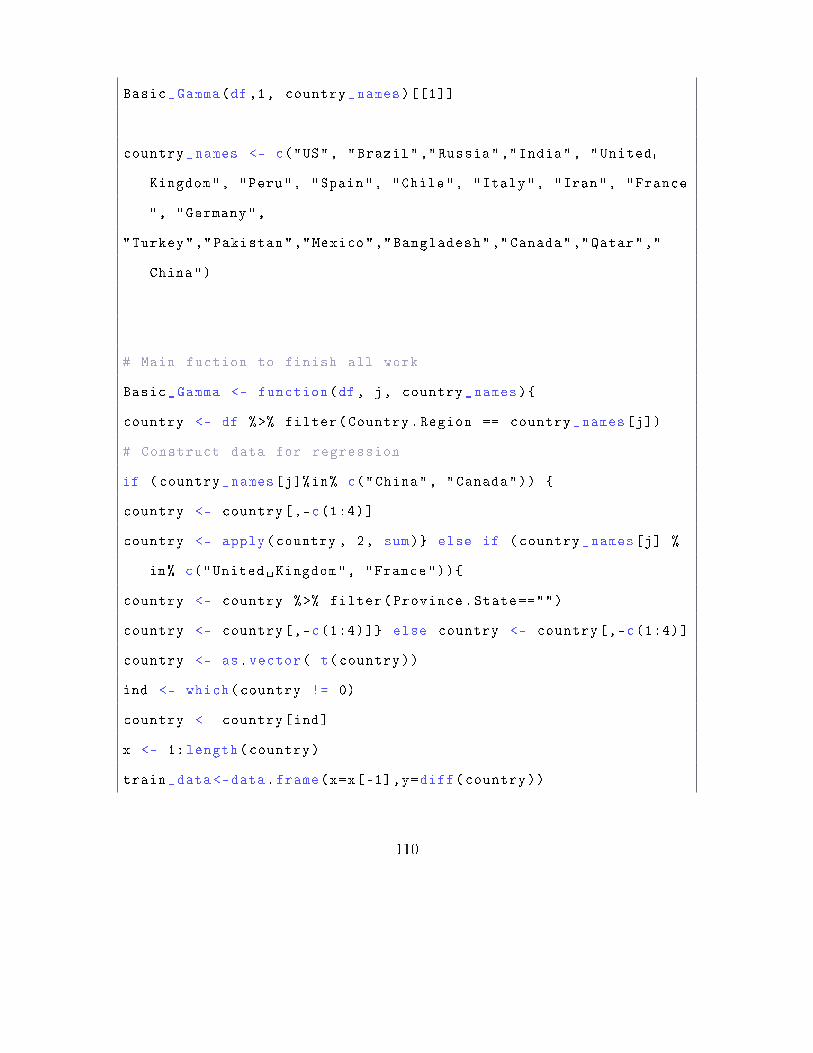
Basic_Gamma(df ,1, country_names)[[1]]
country_names <- c("US", "Brazil","Russia","India", "United
Kingdom", "Peru", "Spain", "Chile", "Italy", "Iran", "France
", "Germany",
"Turkey","Pakistan","Mexico","Bangladesh","Canada","Qatar","
China")
# Main fuction to finish all work
Basic_Gamma <- function(df, j, country_names){
country <- df %>% filter(Country.Region == country_names[j])
# Construct data for regression
if (country_names[j]%in% c("China", "Canada")) {
country <- country[,-c(1:4)]
country <- apply(country , 2, sum)} else if (country_names[j] %
in% c("United Kingdom", "France")){
country <- country %>% filter(Province.State=="")
country <- country[,-c(1:4)]} else country <- country[,-c(1:4)]
country <- as.vector( t(country))
ind <- which(country != 0)
country <- country[ind]
x <- 1: length(country)
train_data <-data.frame(x=x[-1],y=diff(country))
110

# Load initial coefficient of correspond country
wsp_gam <- coef_gam[j,]
# Estimate the coefficients in basic gamma distribution by nls
()
mod_gam <- nls(y ~ a * x^(b-1)*exp(-x/c) / (c^b*gamma(b)), data
= data.frame(y=diff(country), x=x[-1]),
start = list(a = wsp_gam[1], b = wsp_gam[2], c=wsp_gam [3]),
control=nls.control(maxiter = 10000, tol = 1e-05, minFactor = 1
/1024, printEval = FALSE , warnOnly = FALSE),
algorithm = "port")
# Construct data frame to save the real data
data_diff <- data_cum <- NULL
day <- as.Date("22 -01 -2020", format="%d-%m-%Y")+0:( length(
country) -1)+min(ind)-1
total <- as.vector(country)
data_cum <- data.frame(day , total , type=rep("real", length(
country)))
data_diff <- data.frame(day=day[-1], growth=diff(total), type=
rep("real", length(country) -1))
# Construct data frame to save the prediction result
111
t<-0:200
s <- min(ind)-1
wsp_gam <- coef(mod_gam)
wsp_list <-c(wsp_gam[1],wsp_gam[2],wsp_gam [3])
data_cum <- rbind(data_cum , data.frame(day = as.Date("
22 -01 -2020", format="%d-%m-%Y")+t+s,
total=wsp_gam[1]*pgamma(t, shape = wsp_gam[2],
scale = wsp_gam [3]),
type=rep("scaled Gamma", length(t))))
data_diff <- rbind(data_diff , data.frame(day = as.Date("
22 -01 -2020", format="%d-%m-%Y")+t-1+s,
growth=wsp_gam[1]*dgamma(t, shape = wsp_gam[2],
scale = wsp_gam [3]),
type=rep("scaled Gamma", length(t))))
library(scales)
library(plotly)
112

#Construct data frame for ploting the prediction curve and real
value data of total confirmed cases
real_cum <-data_cum[which(data_cum$type=='real'),]
gamma_cum <-data_cum[which(data_cum$type=='scaled Gamma'),]
c<-NA
for (i in 1:( length(gamma_cum$day)-length(real_cum$day) -1)) {
c<-c(c,NA)
}
real_cum_data <-c(real_cum$total ,c)
plot_cum_data <-data.frame(day=gamma_cum$day ,scaled=gamma_cum$
total ,real=real_cum_data)
#Construct data frame for ploting the prediction curve and real
value data of daily growth cases
real_diff <-data_diff[which(data_diff$type=='real'),]
gamma_diff <-data_diff[which(data_diff$type=='scaled Gamma'),]
d<-NA
for (i in 1:( length(gamma_diff$day)-length(real_diff$day) -1)) {
d<-c(d,NA)
}
real_diff_data <-c(real_diff$growth ,d)
plot_diff_data <-data.frame(day=gamma_diff$day ,scaled=gamma_diff
$growth ,real=real_diff_data)
113

# Date of Mean
mean_value <-mean(real_diff$growth)
index1 <-max(c(which(abs(mean_value -real_diff$growth)==min(abs(
mean_value -real_diff$growth)))))
mean_date <-real_diff$day[index1]
# Date of Median
median_value <-median(real_diff$growth)
index2 <-max(c(which(abs(median_value -real_diff$growth)==min(abs
(median_value -real_diff$growth)))))
median_date <-real_diff$day[index2]
# Date of Maximum
max_value <-max(real_diff$growth)
max_date <-real_diff[which(real_diff$growth ==max_value) ,1]
#Save all dates in a list
all_dates <-list(mean_date ,median_date ,max_date)
# Draw Vertical Line
vline <- function(x = 0, color = "red") {
list(
type = "line",
y0 = 0,
114
y1 = 1,
yref = "paper",
x0 = x,
x1 = x,
line = list(color = color ,dash="dash")
)
}
#Plot the prediction curve and real value data of total
confirmed cases
fig_cum <-plot_ly(plot_cum_data ,x=~day ,y=~scaled ,name = 'Total
Prediction ',type = 'scatter ',mode='lines')
fig_cum <-fig_cum%>%add_trace(y=~real ,name='Toal Real',mode='
markers ')
fig_cum <-fig_cum%>%layout(title=paste("Total confirmed in",
country_names[j]),
xaxis=list(title="Date"),
yaxis=list(title="Total"))
#fig_cum <-fig_cum%>%layout(shapes=list(vline(mean_date ,color =
'rgb(22, 96, 167) '),vline(median_date ,color = 'rgb(205, 12,
24) '),vline(max_date ,"Green")))
#Plot the curve of real value of total confirmed cases
115

fig_real_cum <-plot_ly(real_cum ,x=~real_cum$day ,y=~real_cum$
total ,name = 'Real Total Confirmed ',type = 'scatter ',mode='
lines+markers ')
fig_real_cum <-fig_real_cum%>%layout(title=paste("Real Total
Confirmed in", country_names[j]),
xaxis=list(title="Date"),
yaxis=list(title="Total"))
#Plot the prediction curve and real value data of daily growth
cases
fig_diff <-plot_ly(plot_diff_data ,x=~day ,y=~scaled ,name = 'Daily
Prediction ',type = 'scatter ',mode='lines')
fig_diff <-fig_diff%>%add_trace(y=~real ,name='Daily Real',mode='
markers ')
fig_diff <-fig_diff%>%layout(title=paste("Daily growth in",
country_names[j]),
xaxis=list(title="Date"),
yaxis=list(title="Growth"))
#fig_diff <-fig_diff%>%layout(shapes=list(vline(mean_date ,color
= 'rgb(22, 96, 167) '),vline(median_date ,color = 'rgb(205,
12, 24) '),vline(max_date ,"Green")))
116

#Plot the curve of real value of daily growth cases
fig_real_diff <-plot_ly(real_diff ,x=~real_diff$day ,y=~real_diff$
growth ,name = 'Real Daily Grwoth ',type = 'scatter ',mode='
lines+markers ')
fig_real_diff <-fig_real_diff%>%layout(title=paste("Real Daily
Growth in", country_names[j]),
xaxis=list(title="Date"),
yaxis=list(title="Growth"))
#Stitch the plot of total confirmed prediction with plot of
daily growth prediction
fig_nail <-subplot(fig_cum ,fig_diff ,nrows = 2)
fig_nail <-fig_nail%>%layout(title=paste("Cases in",country_
names[j]))
#Stitch the plot of real total confirmed with plot of real
daily growth
fig_nail_real <-subplot(fig_real_cum ,fig_real_diff ,nrows = 2)
fig_nail_real <-fig_nail_real%>%layout(title=paste("Real Cases
in",country_names[j]))
return(list(fig_nail ,all_dates ,summary(mod_gam)))}
117

C Application Gamma Prediction Model R Program
rm(list=ls())
library(openxlsx)
library(dplyr)
library(pracma)
library(plotly)
library(RCurl)
options(scipen = 200)
# Load original data from GitHub to data frame
raw_data <-getURL("https://raw.githubusercontent.com/
CSSEGISandData/COVID -19/master/csse_covid_19_data/csse_covid
_19_time_series/time_series_covid19_confirmed_global.csv")
df <- read.csv(text=raw_data)
# Construct data for regression
iran <- df %>% filter(Country.Region == "Iran")
iran <- as.vector(t(iran[,-c(1:4)]))
ind <-iran[which(iran!=0)]
x<-1: length(iran)
# Load data of initial coefficient
wsp_gam <- c(186855 , 63.6, 2.01, 23, 3.2)
118

# Estimate the coefficients in gamma distribution by nls()
mod_gam2 <- nls(y ~ a/2 * (x^(b-1)*exp(-x/c) / (c^b*gamma(b)) +
x^(d-1)*exp(-x/e) / (e^d*gamma(d))),
data = data.frame(y=c( iran[1],diff(iran)), x=x),
start = list(a = wsp_gam[1], b = wsp_gam[2], c=wsp_gam[3], d=
wsp_gam[4], e=wsp_gam [5]),
control=nls.control(maxiter = 10000, tol = 1e-05, minFactor = 1
/1024, printEval = FALSE , warnOnly = FALSE),
algorithm = "port")
# Construct data frame to save the real data
data_diff <-data_cum <-NULL
day <-as.Date("22 -01 -2020", format="%d-%m-%Y")+0:( length(iran)
-1)+min(ind)-1
total <- as.vector(iran)
data_cum <- data.frame(day , total , type=rep("real", length(iran
)))
data_diff <- data.frame(day=day[-1], growth=diff(total), type=
rep("real", length(iran) -1))
#Construct data frame to save the prediction result
t <- 0:180
s <- min(ind)-1
wsp_gam2 <- coef(mod_gam2)
119

a <- wsp_gam2 [1]
b <- wsp_gam2 [2]
c <- wsp_gam2 [3]
d <- wsp_gam2 [4]
e <- wsp_gam2 [5]
daily_prediction <-a /2 * (t^(b-1)*exp(-t/c) / (c^b*gamma(b)) +
t^(d-1)*exp(-t/e) / (e^d*gamma(d)))
data_cum <- rbind(data_cum , data.frame(day = as.Date("
22 -01 -2020", format="%d-%m-%Y")+t+s,
total=cumsum(daily_prediction),
type=rep("scaled Gamma", length(t))))
data_diff <- rbind(data_diff , data.frame(day = as.Date("
22 -01 -2020", format="%d-%m-%Y")+t-1+s,
growth=daily_prediction ,
type=rep("scaled Gamma", length(t))))
library(scales)
#Construct data frame for ploting the prediction curve and real
value data of total confirmed cases
real_cum <-data_cum[which(data_cum$type=='real'),]
gamma_cum <-data_cum[which(data_cum$type=='scaled Gamma'),]
blank <-NA
120

for (i in 1:( length(gamma_cum$day)-length(real_cum$day) -1)) {
blank <-c(blank ,NA)
}
real_cum_data <-c(real_cum$total ,blank)
plot_cum_data <-data.frame(day=gamma_cum$day ,scaled=gamma_cum$
total ,real=real_cum_data)
#Plot the prediction curve and real value data of total
confirmed cases
fig_cum <-plot_ly(plot_cum_data ,x=~day ,y=~scaled ,name = 'Total
Prediction ',type = 'scatter ',mode='lines')
fig_cum <-fig_cum%>%add_trace(y=~real ,name='Toal Real',mode='
markers ')
fig_cum <-fig_cum%>%layout(title=paste("Total confirmed in Iran"
),
xaxis=list(title="Date"),
yaxis=list(title="Total"))
fig_cum <-fig_cum%>%layout(shapes=list(vline(mean_date ,color = '
rgb(22, 96, 167)'),vline(median_date ,color = 'rgb(205, 12,
24)'),vline(max_date ,"Green")))
121

#Construct data frame for ploting the prediction curve and real
value data of daily growth cases
real_diff <-data_diff[which(data_diff$type=='real'),]
gamma_diff <-data_diff[which(data_diff$type=='scaled Gamma'),]
blank2 <-NA
for (i in 1:( length(gamma_diff$day)-length(real_diff$day) -1)) {
blank2 <-c(blank2 ,NA)
}
real_diff_data <-c(real_diff$growth ,blank2)
plot_diff_data <-data.frame(day=gamma_diff$day ,scaled=gamma_diff
$growth ,real=real_diff_data)
#Plot the prediction curve and real value data of daily growth
cases
fig_diff <-plot_ly(plot_diff_data ,x=~day ,y=~scaled ,name = 'Daily
Prediction ',type = 'scatter ',mode='lines')
fig_diff <-fig_diff%>%add_trace(y=~real ,name='Daily Real',mode='
markers ')
fig_diff <-fig_diff%>%layout(title=paste("Daily growth in Iran")
,
xaxis=list(title="Date"),
yaxis=list(title="Growth"))
fig_diff <-fig_diff%>%layout(shapes=list(vline(mean_date ,color =
'rgb(22, 96, 167)'),vline(median_date ,color = 'rgb(205, 12,
122

24)'),vline(max_date ,"Green")))
#Stitch the plot of total confirmed prediction with plot of
daily growth prediction
fig_nail <-subplot(fig_cum ,fig_diff ,nrows = 2)
fig_nail <-fig_nail%>%layout(title=paste("Cases in Iran"))
fig_nail
# Date of Mean
mean_value <-mean(real_diff$growth)
index1 <-max(c(which(abs(mean_value -real_diff$growth)==min(abs(
mean_value -real_diff$growth)))))
mean_date <-real_diff$day[index1]
# Date of Median
median_value <-median(real_diff$growth)
index2 <-max(c(which(abs(median_value -real_diff$growth)==min(abs
(median_value -real_diff$growth)))))
median_date <-real_diff$day[index2]
# Date of Maximum
123

max_value <-max(real_diff$growth)
max_date <-real_diff[which(real_diff$growth ==max_value) ,1]
# Draw Vertical Line
vline <- function(x = 0, color = "red") {
list(
type = "line",
y0 = 0,
y1 = 1,
yref = "paper",
x0 = x,
x1 = x,
line = list(color = color ,dash="dash")
)
}
124
Top Related