


Languages
Pages
Legal

Footprints: outlineÜllar Rannik
University of Helsinki
-Concept of footprint and definitions-Analytical footprint models-Model by Korman and Meixner-Footprints for fluxes vs. concentrations-Footprints for gradient and profile techniques-Footprint evaluation other methods-Lagrangian stochastic models
-Vegatated canopies-Inhomogeneos flows and complex terrain
•No too detailed derivations
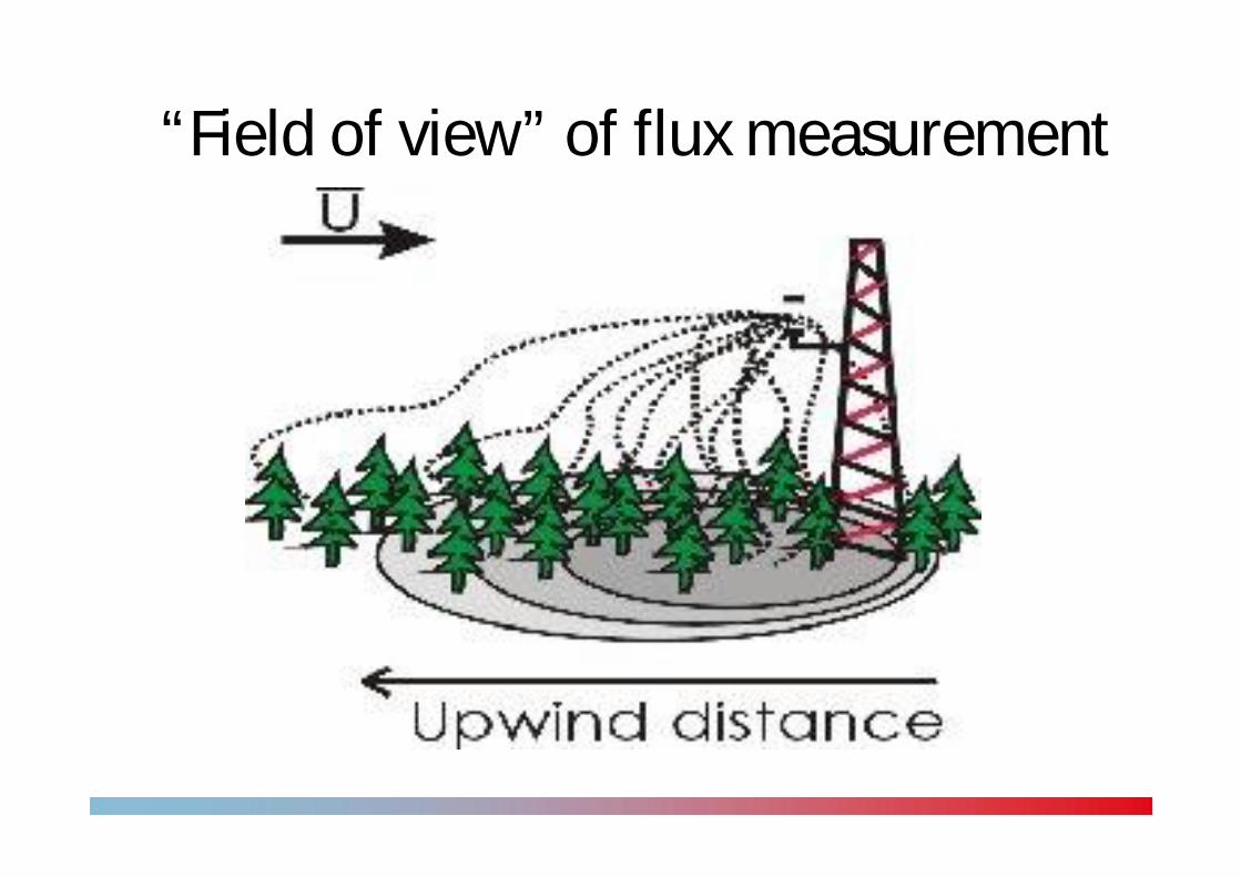
“Field of view” of flux measurement
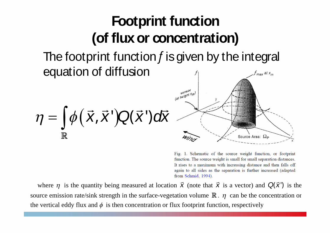
Footprint function(of flux or concentration)
The footprint function f is given by the integral equation of diffusion
, ' ( ') 'x x Q x dx
where is the quantity being measured at location x (note that x is a vector) and ( ')Q x is the source emission rate/sink strength in the surface-vegetation volume can be the concentration or the vertical eddy flux and is then concentration or flux footprint function, respectively
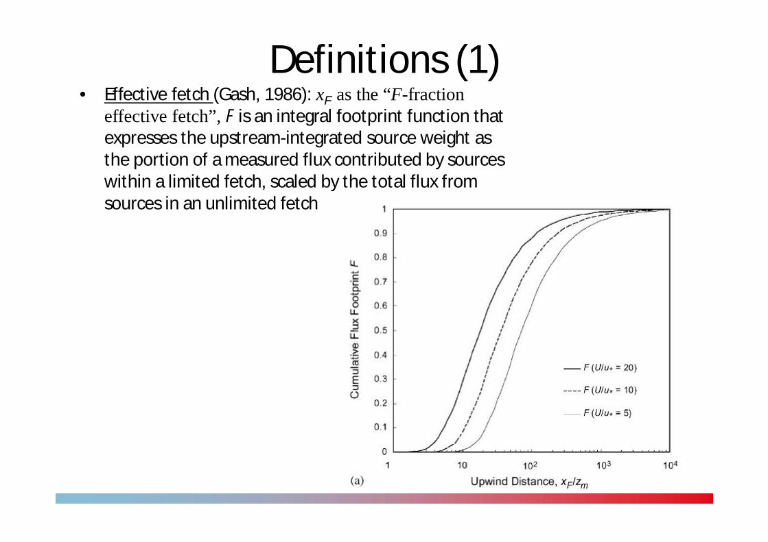
Definitions (1)• Effective fetch (Gash, 1986): xF as the “F-fraction
effective fetch”, F is an integral footprint function that expresses the upstream-integrated source weight as the portion of a measured flux contributed by sources within a limited fetch, scaled by the total flux from sources in an unlimited fetch
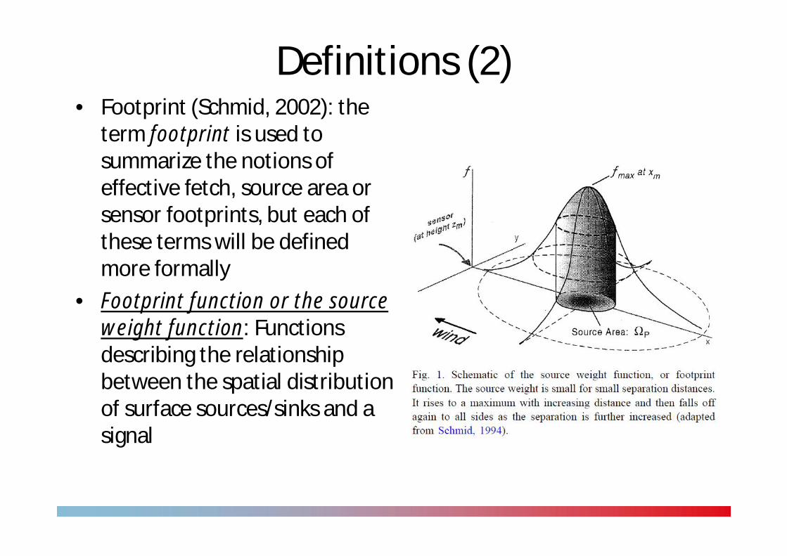
Definitions (2)• Footprint (Schmid, 2002): the
term footprint is used to summarize the notions of effective fetch, source area or sensor footprints, but each of these terms will be defined more formally
• Footprint function or the source weight function: Functions describing the relationship between the spatial distribution of surface sources/sinks and a signal
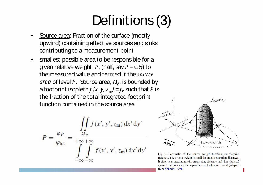
Definitions (3)• Source area: Fraction of the surface (mostly
upwind) containing effective sources and sinks contributing to a measurement point
• smallest possible area to be responsible for a given relative weight, P, (half, say P = 0.5) to the measured value and termed it the source area of level P. Source area, P, is bounded by a footprint isopleth f (x, y, zm) = fP such that P is the fraction of the total integrated footprint function contained in the source area
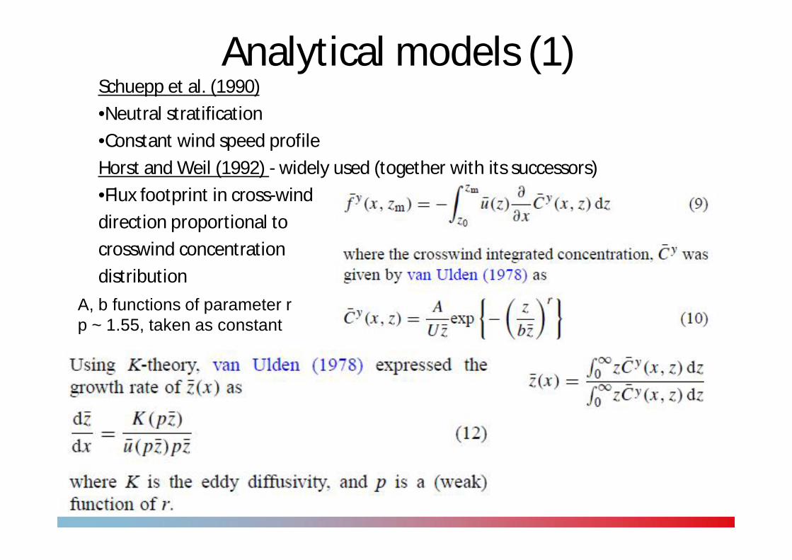
Analytical models (1)Schuepp et al. (1990)•Neutral stratification•Constant wind speed profileHorst and Weil (1992) - widely used (together with its successors)•Flux footprint in cross-wind direction proportional to crosswind concentration distribution
•A•Model implicit in x by mean plume height
A, b functions of parameter rp ~ 1.55, taken as constant
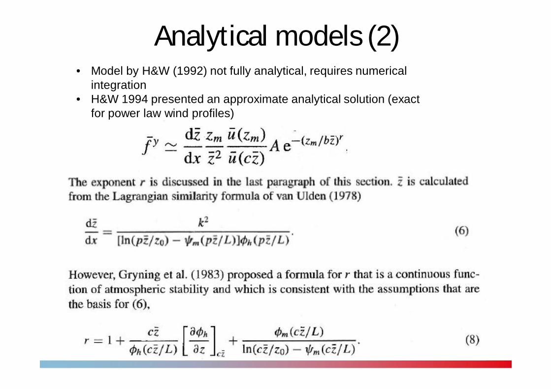
Analytical models (2)• Model by H&W (1992) not fully analytical, requires numerical
integration• H&W 1994 presented an approximate analytical solution (exact
for power law wind profiles)
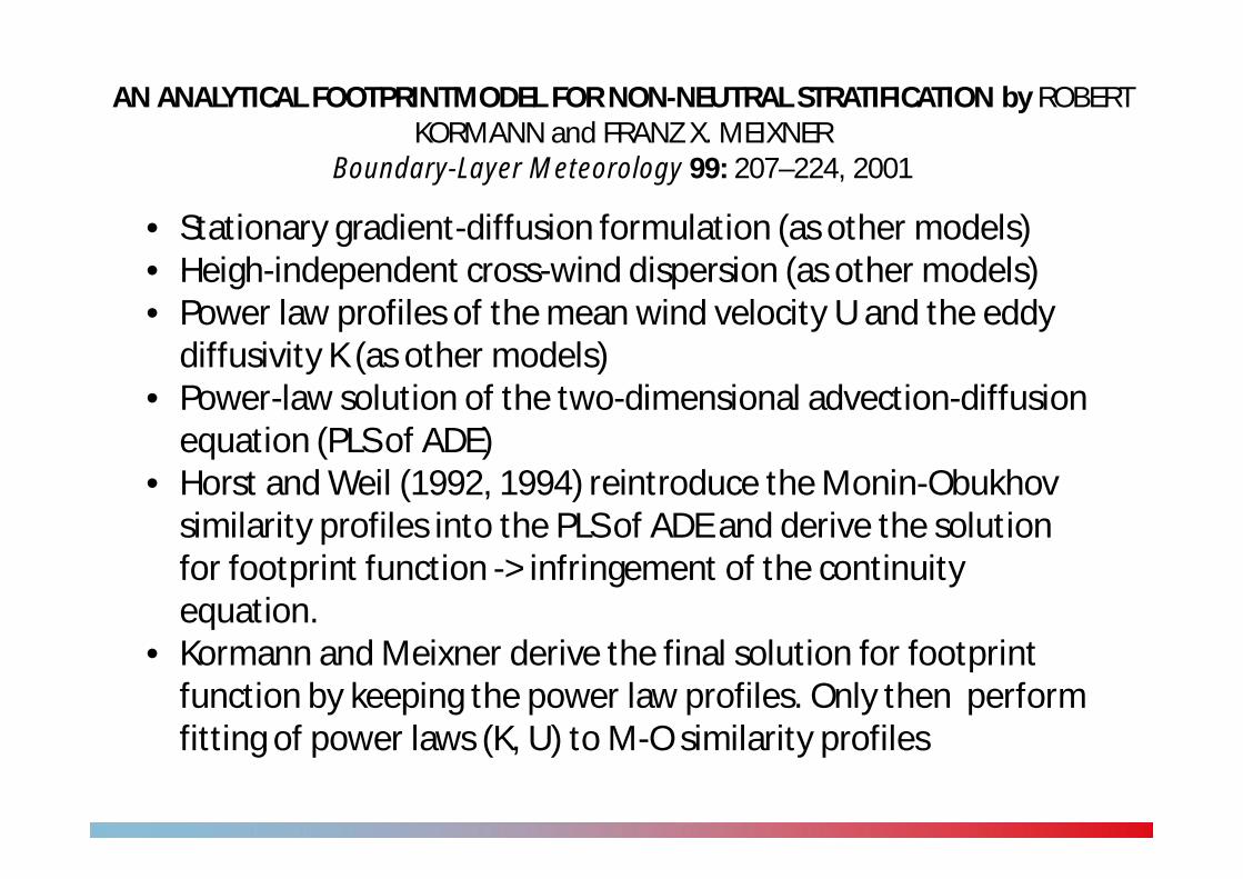
AN ANALYTICAL FOOTPRINTMODEL FOR NON-NEUTRAL STRATIFICATION by ROBERT KORMANN and FRANZ X. MEIXNER
Boundary-Layer Meteorology 99: 207–224, 2001
• Stationary gradient-diffusion formulation (as other models)• Heigh-independent cross-wind dispersion (as other models)• Power law profiles of the mean wind velocity U and the eddy
diffusivity K (as other models)• Power-law solution of the two-dimensional advection-diffusion
equation (PLS of ADE)• Horst and Weil (1992, 1994) reintroduce the Monin-Obukhov
similarity profiles into the PLS of ADE and derive the solution for footprint function -> infringement of the continuity equation.
• Kormann and Meixner derive the final solution for footprint function by keeping the power law profiles. Only then perform fitting of power laws (K, U) to M-O similarity profiles
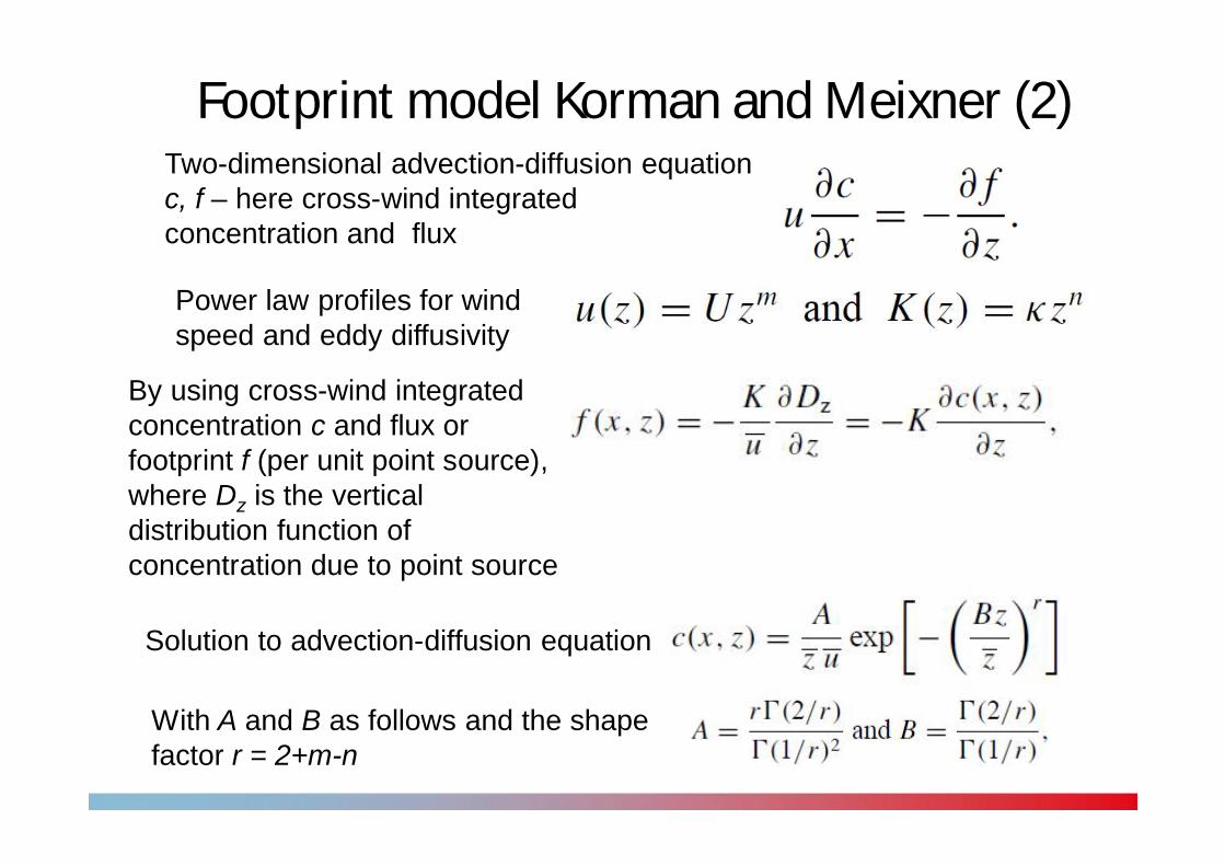
Footprint model Korman and Meixner (2)
Power law profiles for wind speed and eddy diffusivity
Two-dimensional advection-diffusion equationc, f – here cross-wind integrated concentration and flux
By using cross-wind integrated concentration c and flux or footprint f (per unit point source), where Dz is the vertical distribution function of concentration due to point source
Solution to advection-diffusion equation
With A and B as follows and the shape factor r = 2+m-n
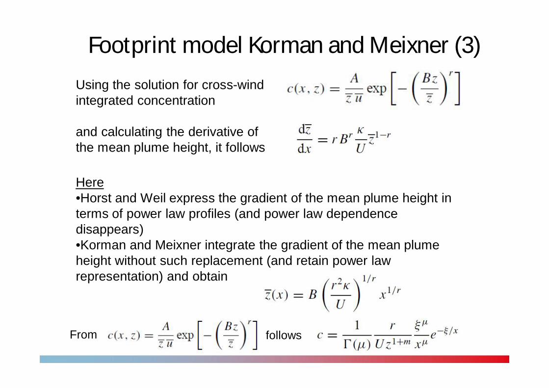
Footprint model Korman and Meixner (3)Using the solution for cross-wind integrated concentration
and calculating the derivative of the mean plume height, it follows
Here •Horst and Weil express the gradient of the mean plume height in terms of power law profiles (and power law dependence disappears)•Korman and Meixner integrate the gradient of the mean plume height without such replacement (and retain power law representation) and obtain
From follows
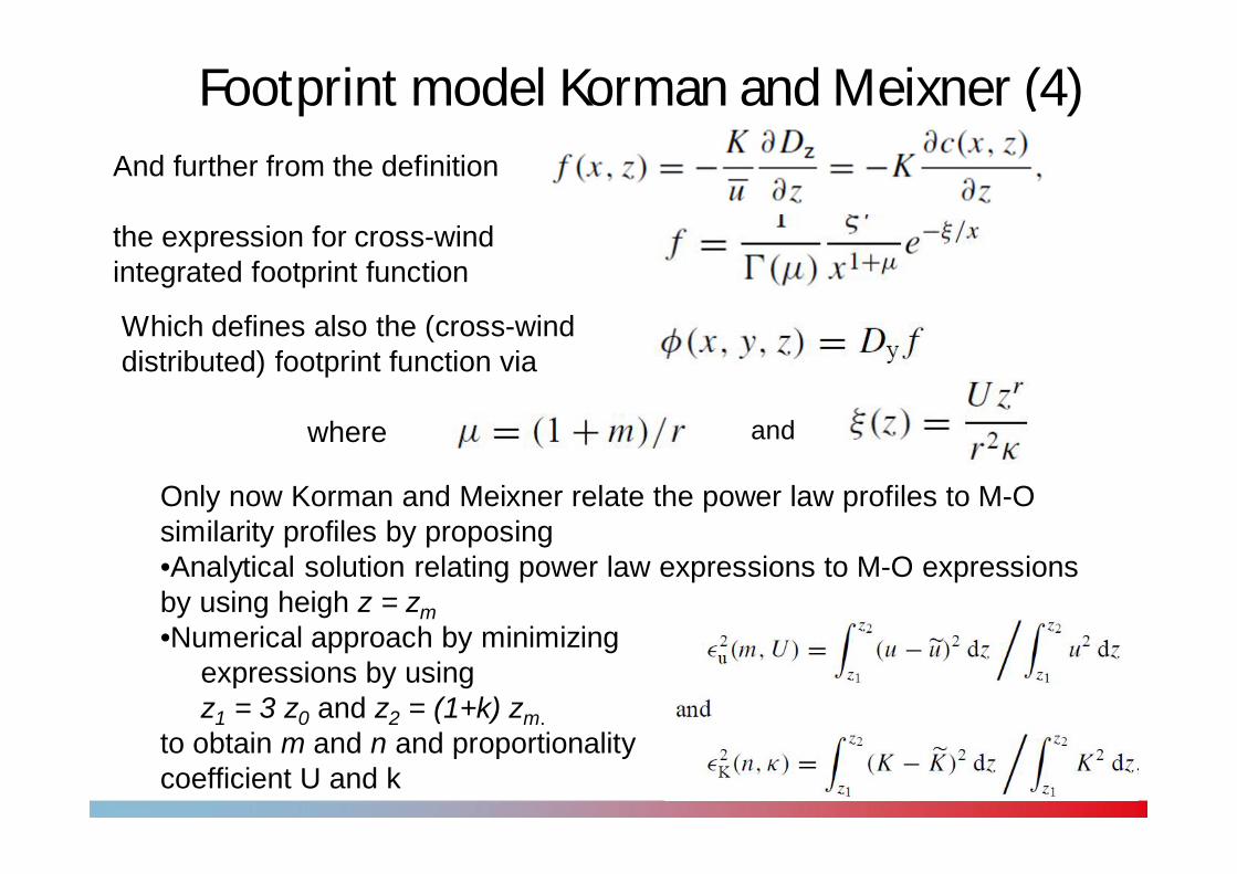
Footprint model Korman and Meixner (4)And further from the definition
the expression for cross-wind integrated footprint function
Which defines also the (cross-wind distributed) footprint function via
where and
Only now Korman and Meixner relate the power law profiles to M-O similarity profiles by proposing•Analytical solution relating power law expressions to M-O expressions by using heigh z = zm•Numerical approach by minimizing
expressions by using z1 = 3 z0 and z2 = (1+k) zm.
to obtain m and n and proportionality coefficient U and k
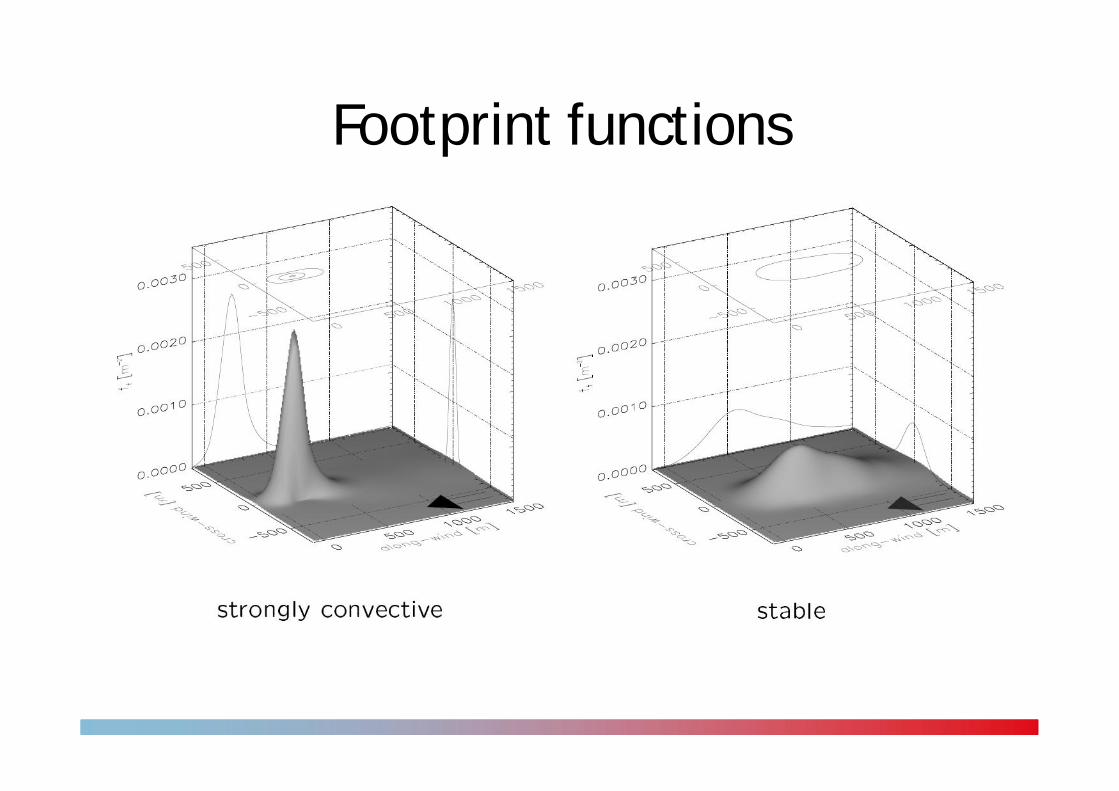
Footprint functions
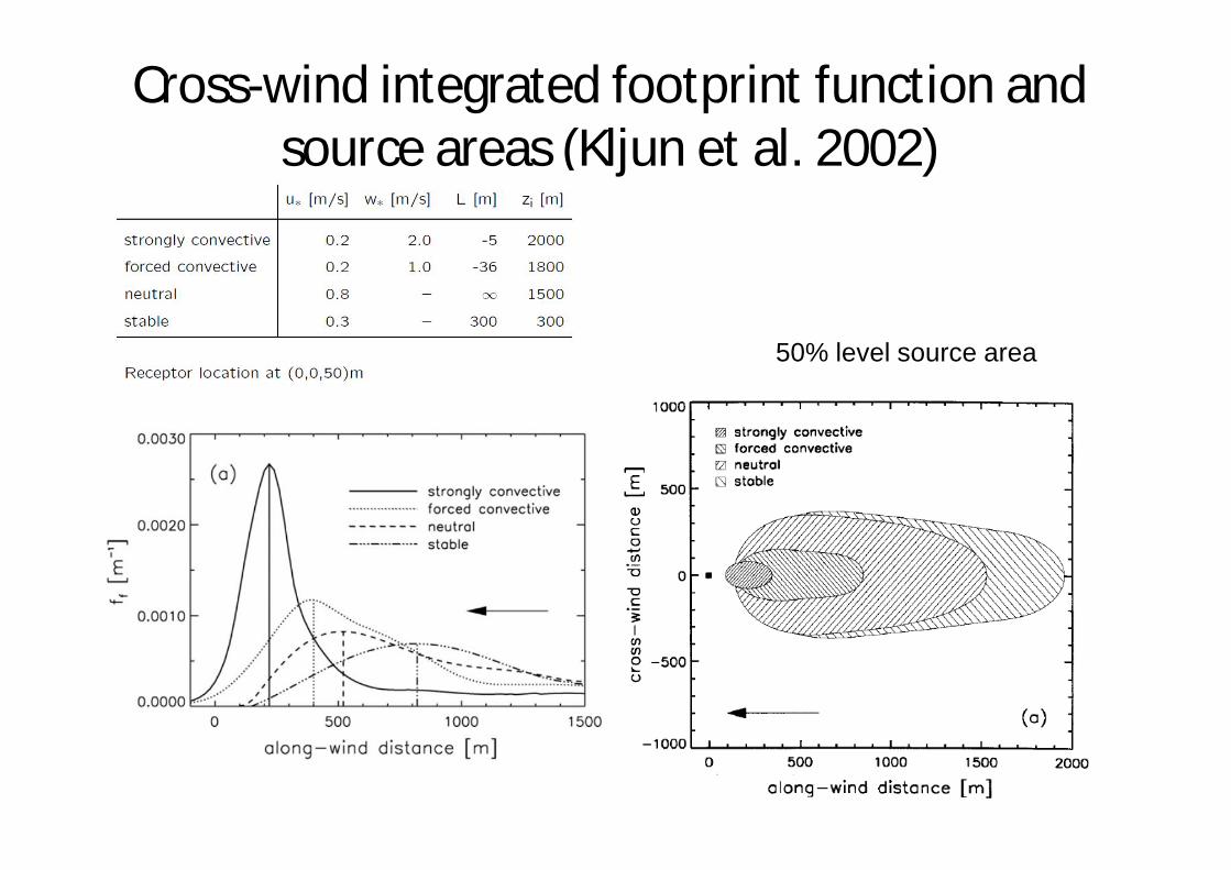
Cross-wind integrated footprint function and source areas (Kljun et al. 2002)
50% level source area
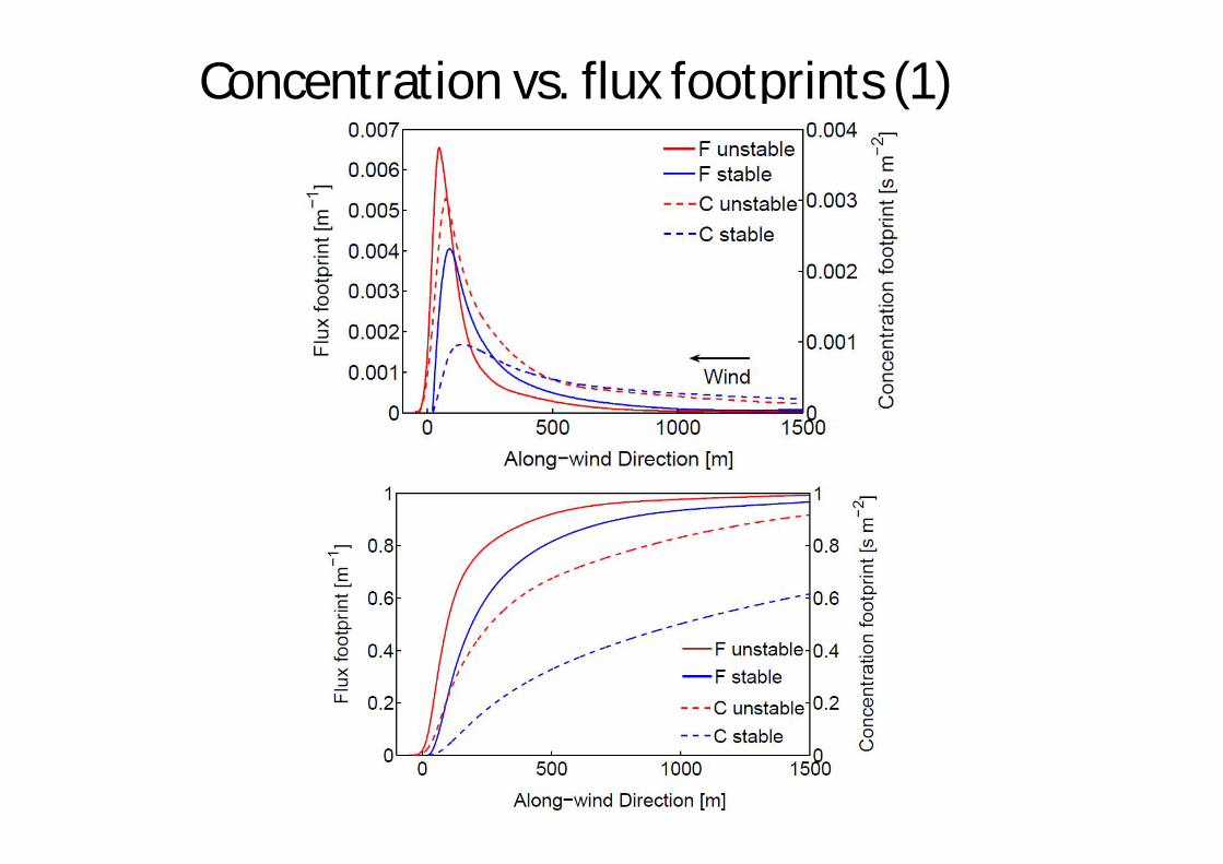
Concentration vs. flux footprints (1)
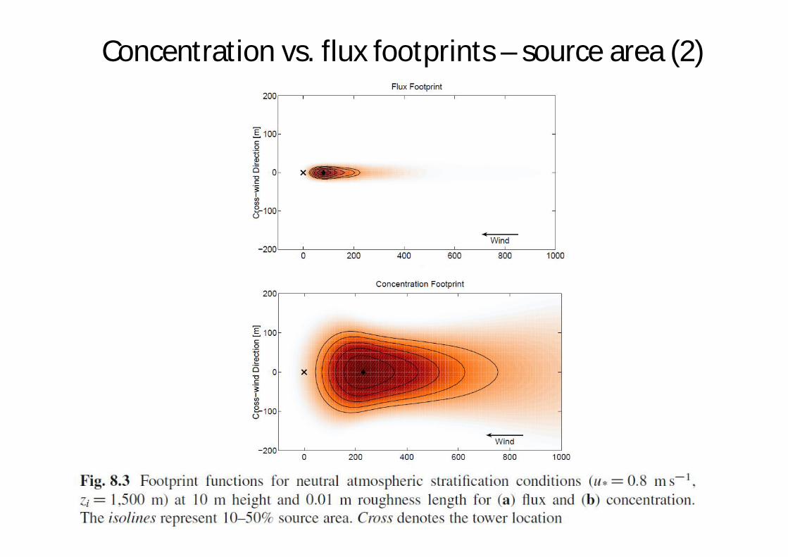
Concentration vs. flux footprints – source area (2)
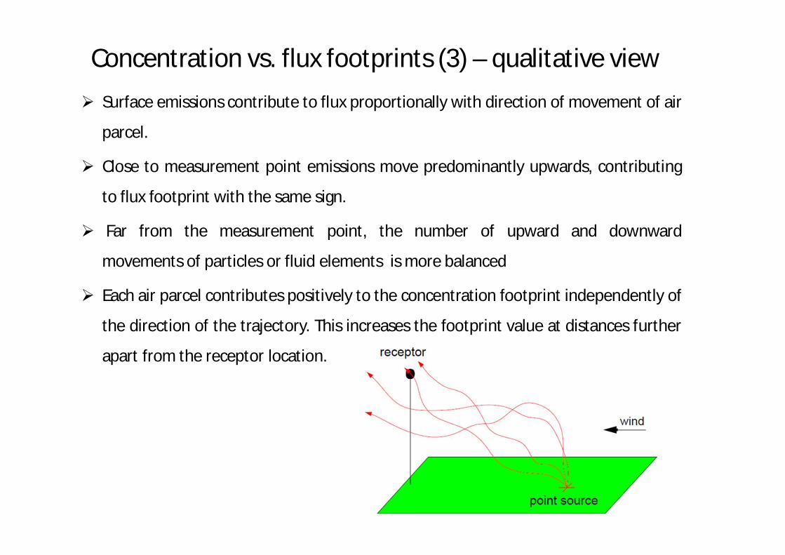
Concentration vs. flux footprints (3) – qualitative viewSurface emissions contribute to flux proportionally with direction of movement of air
parcel.
Close to measurement point emissions move predominantly upwards, contributing
to flux footprint with the same sign.
Far from the measurement point, the number of upward and downward
movements of particles or fluid elements is more balanced
Each air parcel contributes positively to the concentration footprint independently of
the direction of the trajectory. This increases the footprint value at distances further
apart from the receptor location.
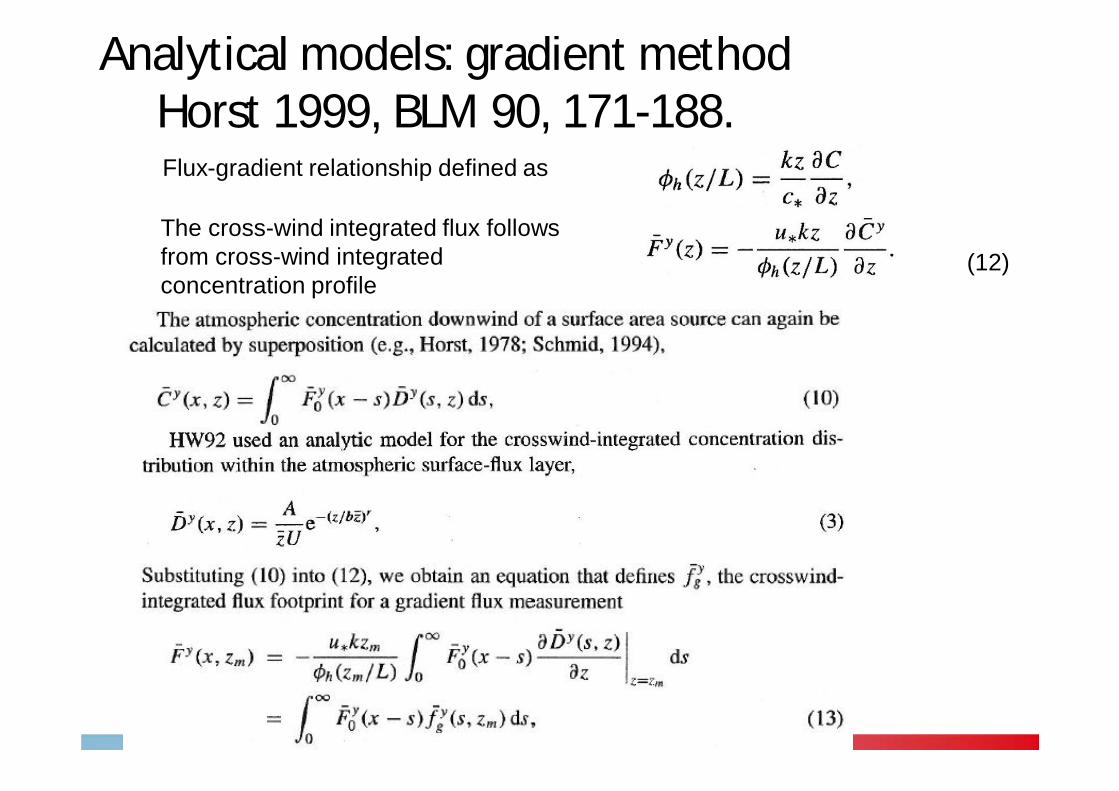
Analytical models: gradient methodHorst 1999, BLM 90, 171-188.Flux-gradient relationship defined as
The cross-wind integrated flux follows from cross-wind integrated concentration profile
(12)
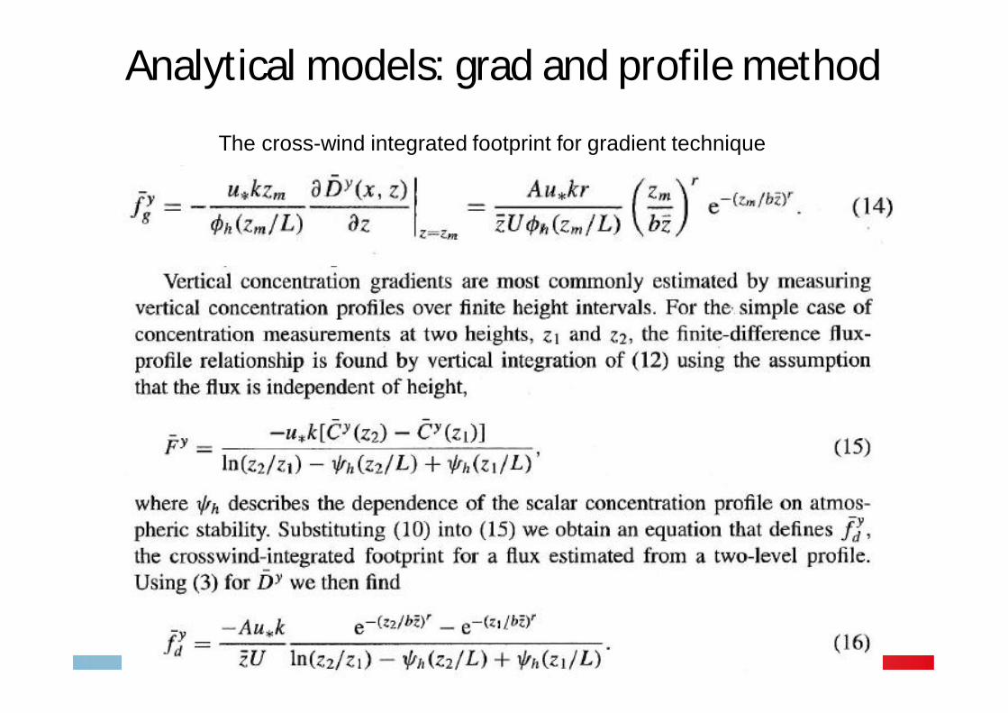
Analytical models: grad and profile method
The cross-wind integrated footprint for gradient technique
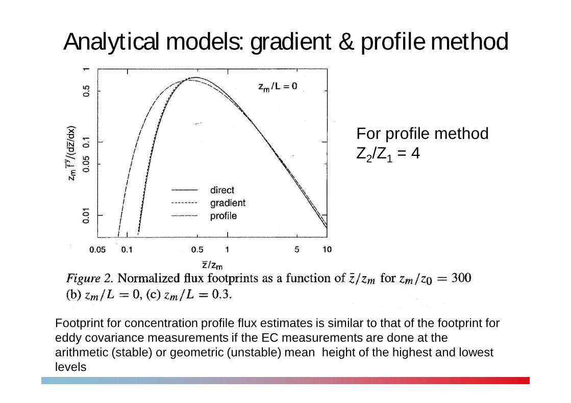
Analytical models: gradient & profile method
Footprint for concentration profile flux estimates is similar to that of the footprint for eddy covariance measurements if the EC measurements are done at the arithmetic (stable) or geometric (unstable) mean height of the highest and lowest levels
For profile method Z2/Z1 = 4
Analytical models summary (6)• assume a horizontally homogeneous turbulence field• assumption of steady-state conditions during the course of
the flux period analyzed• Based on analytical solution to advection-diffusion equation• Based on the Monin-Obukhov similarity theory (being also
applied to the layer of air above the tower)• assume that no contribution to a point flux is possible by
downwind sources (no along-wind turbulent diffusion)• unable to include the influence of non-local forcings to flux
measurements • no along-wind diffusion included
Other types of footprint models• Analytical models
Applicable to Atmospheric Surface Layer parameterisation only
• Lagrangian Stochastic modelsRequire pre-defined turbulence fieldCan be applied to Atmospheric Boundary Layer (ABL) + vegetation canopy + inhomogeneous flow + complex terrain
• Closure model basedCapable to simulate turbulence fieldApplicable to vegetation canopy + inhomogeneous flow + complex terrainCan be combined with LS modelNumerically demanding
• Large Eddy Simulation basedMost advanced model Capable to simulate turbulence fieldApplicable to ABL + vegetation canopy + inhomogeneous flow (+ terrain with limited complexity)Can be combined with LS modelNumerically very demanding
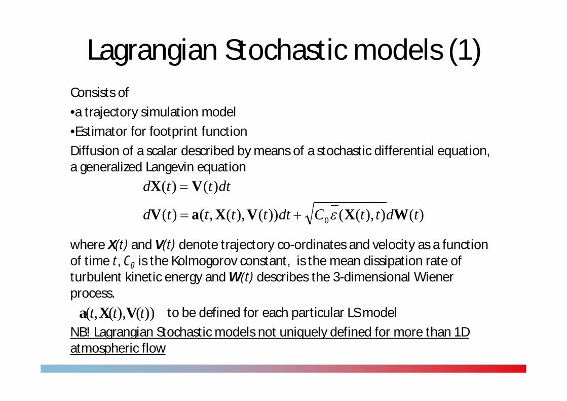
Lagrangian Stochastic models (1)Consists of •a trajectory simulation model•Estimator for footprint functionDiffusion of a scalar described by means of a stochastic differential equation, a generalized Langevin equation
where X(t) and V(t) denote trajectory co-ordinates and velocity as a function of time t, C0 is the Kolmogorov constant, is the mean dissipation rate of turbulent kinetic energy and W(t) describes the 3-dimensional Wiener process.
to be defined for each particular LS modelNB! Lagrangian Stochastic models not uniquely defined for more than 1D atmospheric flow
)()),(())(),(,()(
)()(
0 tdttCdtttttd
dtttd
WXVXaV
VX
))(),(,( ttt VXa
Lagrangian Stochastic models (2)Inputs required by LS trajectory model (Gaussian)•Mean wind speed•Variances of wind speed components•Momentum flux•Dissipation rate of TKE
In addition for non-Gaussian•Skewness of wind speed components (third moments)•Kurtosis of wind speed components (fourth moments)
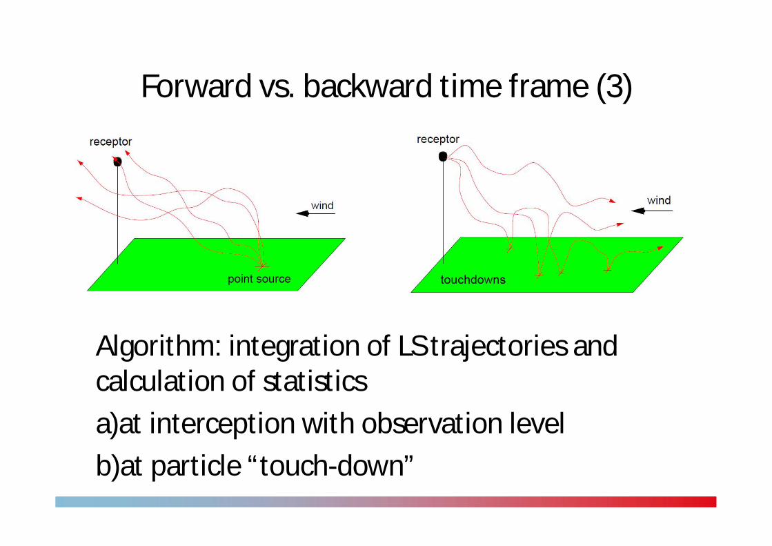
Forward vs. backward time frame (3)
Algorithm: integration of LS trajectories and calculation of statisticsa)at interception with observation levelb)at particle “touch-down”
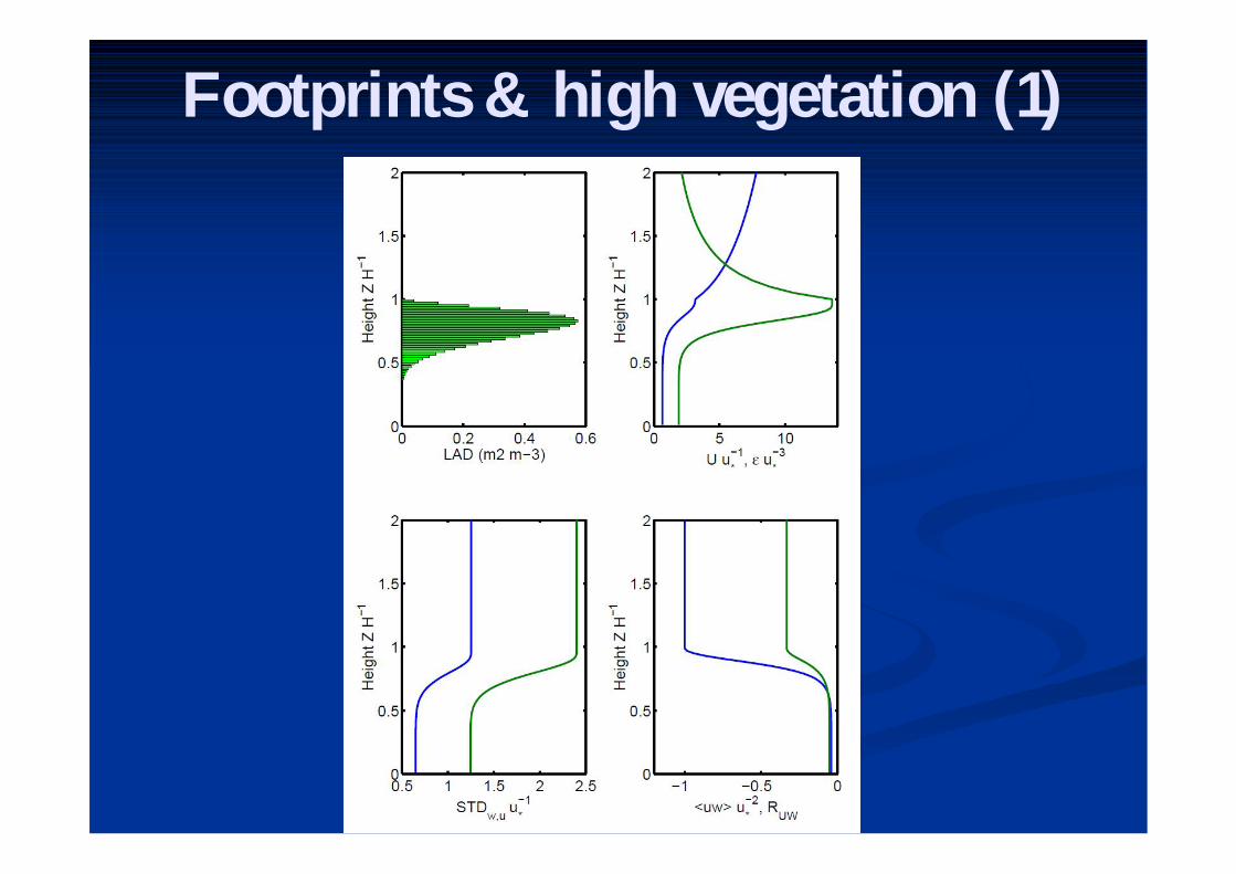
Footprints & high vegetation (1)
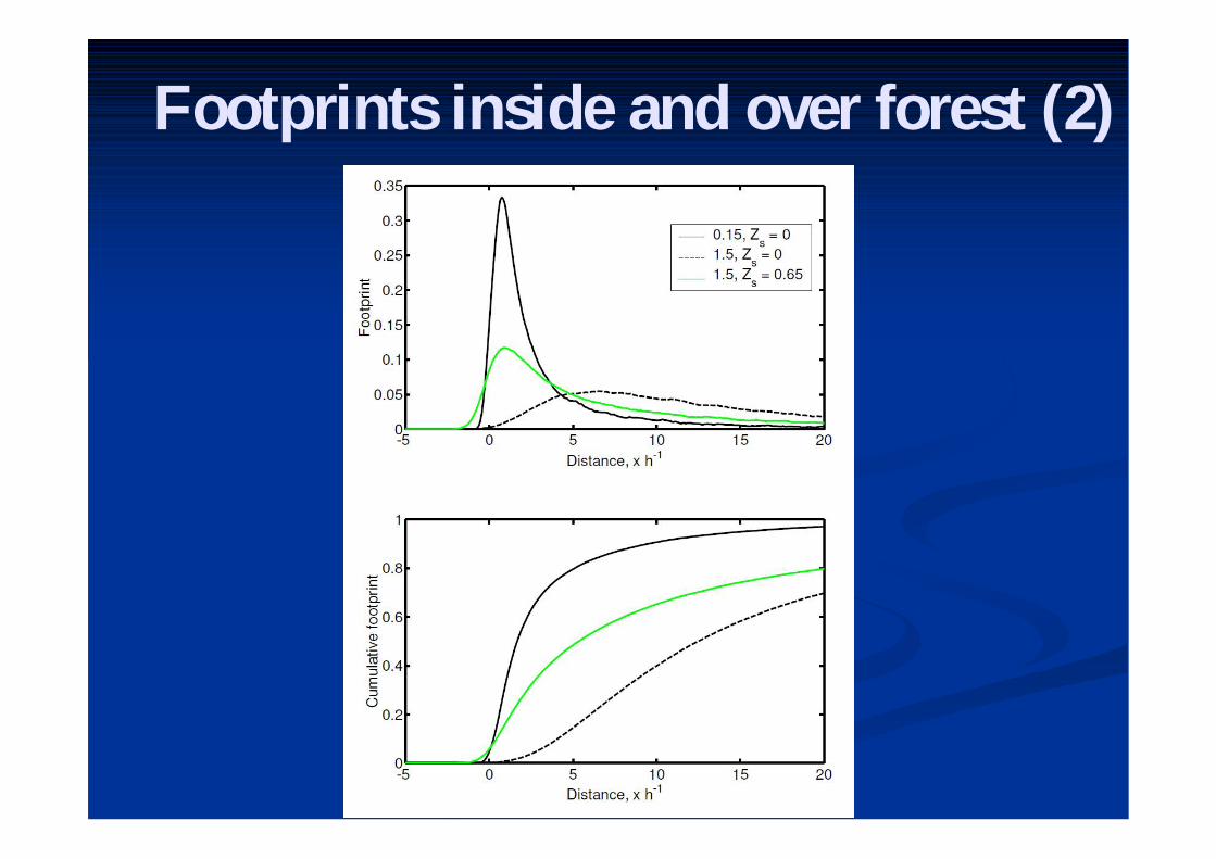
Footprints inside and over forest (2)
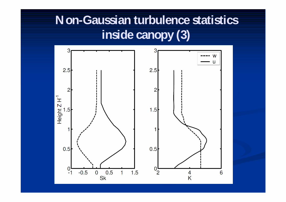
Non-Gaussian turbulence statistics inside canopy (3)
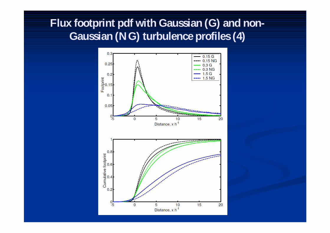
Flux footprint pdf with Gaussian (G) and non-Gaussian (NG) turbulence profiles (4)
Inhomogeneous flow and complex terrain (1)
• Forest canopy inhomogeneity• Complex terrain + vegetation• Urban environment
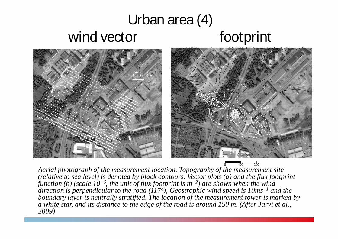
Urban area (4)wind vector footprint
Aerial photograph of the measurement location. Topography of the measurement site (relative to sea level) is denoted by black contours. Vector plots (a) and the flux footprint function (b) (scale 10 6, the unit of flux footprint is m 2) are shown when the wind direction is perpendicular to the road (117o), Geostrophic wind speed is 10ms 1 and the boundary layer is neutrally stratified. The location of the measurement tower is marked by a white star, and its distance to the edge of the road is around 150 m. (After Jarvi et al., 2009)
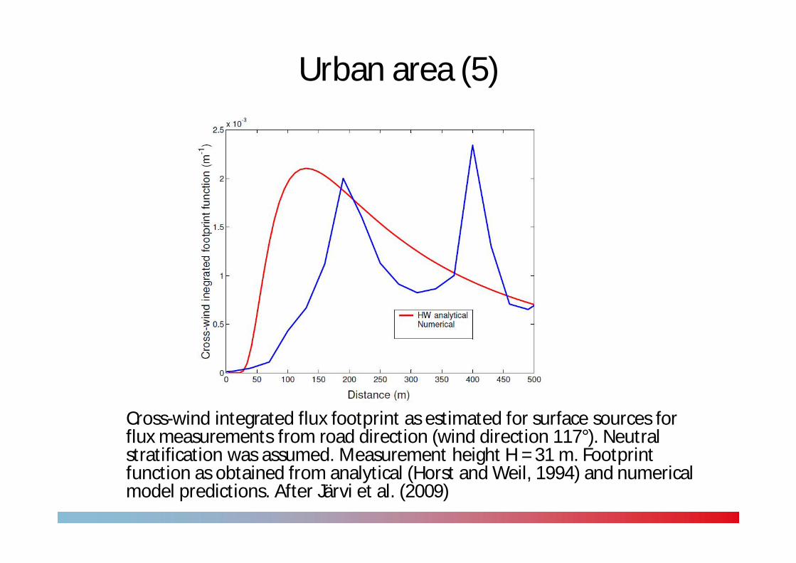
Urban area (5)
Cross-wind integrated flux footprint as estimated for surface sources for flux measurements from road direction (wind direction 117°). Neutral stratification was assumed. Measurement height H = 31 m. Footprint function as obtained from analytical (Horst and Weil, 1994) and numerical model predictions. After Järvi et al. (2009)
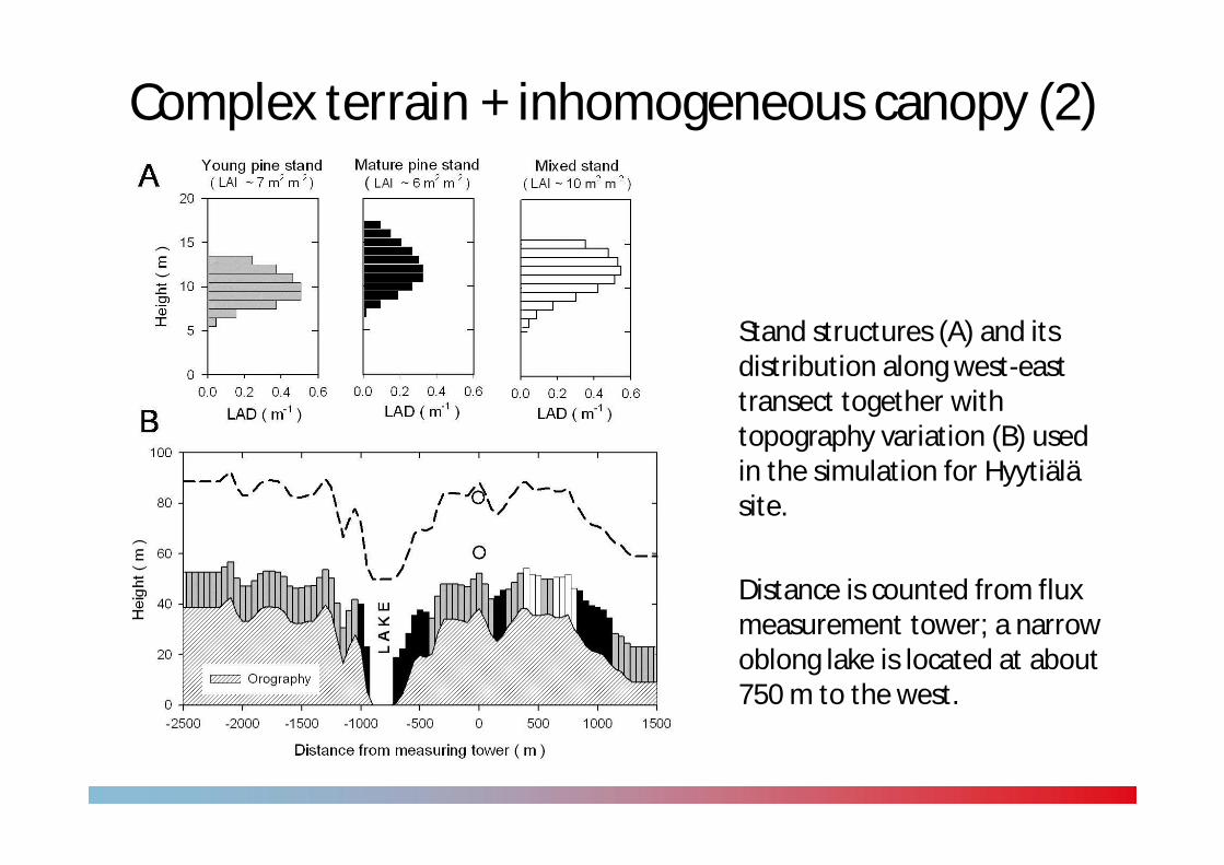
Complex terrain + inhomogeneous canopy (2)
Stand structures (A) and its distribution along west-east transect together with topography variation (B) used in the simulation for Hyytiälä site.
Distance is counted from flux measurement tower; a narrow oblong lake is located at about 750 m to the west.
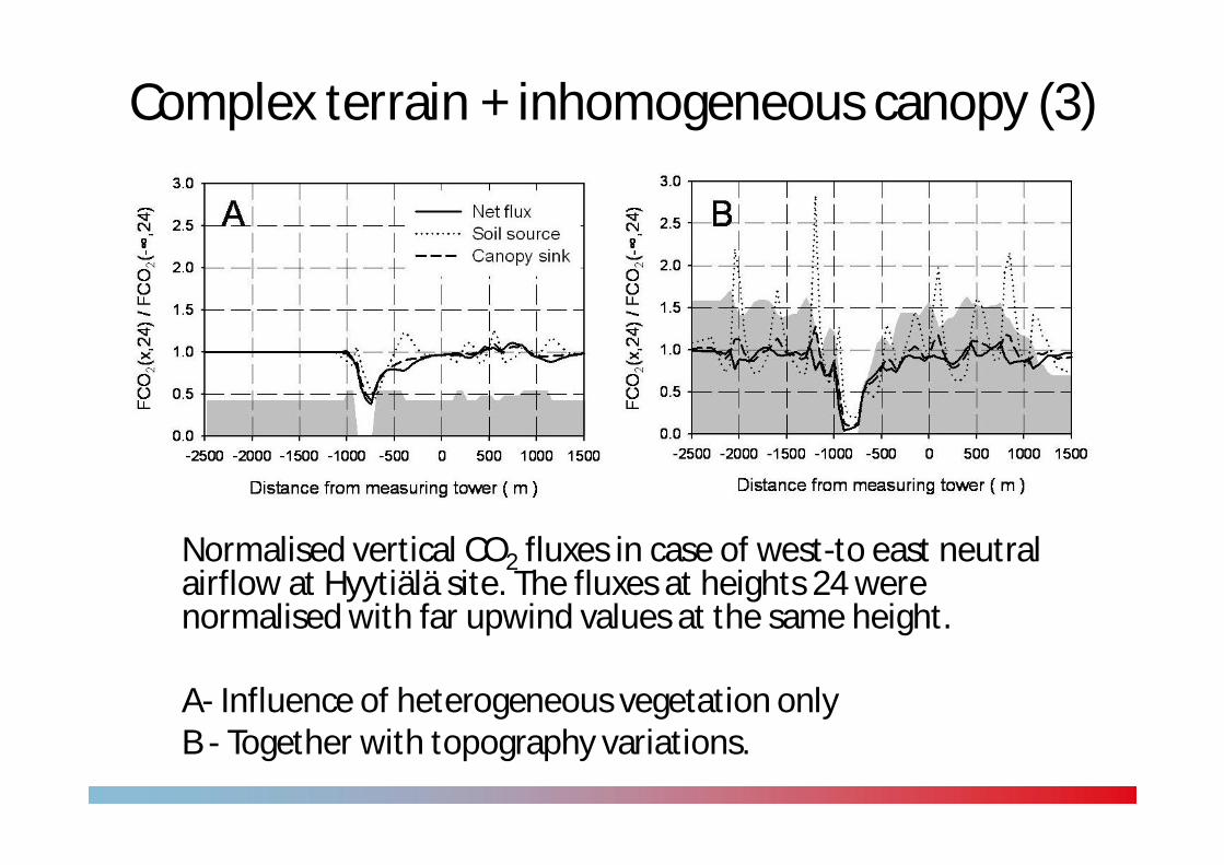
Complex terrain + inhomogeneous canopy (3)
Normalised vertical CO2 fluxes in case of west-to east neutral airflow at Hyytiälä site. The fluxes at heights 24 were normalised with far upwind values at the same height.
A- Influence of heterogeneous vegetation onlyB - Together with topography variations.
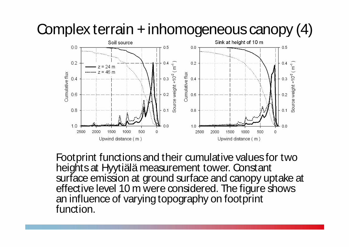
Complex terrain + inhomogeneous canopy (4)
Footprint functions and their cumulative values for two heights at Hyytiälä measurement tower. Constant surface emission at ground surface and canopy uptake at effective level 10 m were considered. The figure shows an influence of varying topography on footprint function.
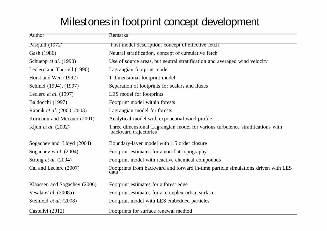
Milestones in footprint concept developmentAuthor Remarks
Pasquill (1972) First model description, concept of effective fetchGash (1986) Neutral stratification, concept of cumulative fetchSchuepp et al. (1990) Use of source areas, but neutral stratification and averaged wind velocity Leclerc and Thurtell (1990) Lagrangian footprint modelHorst and Weil (1992) 1-dimensional footprint modelSchmid (1994), (1997) Separation of footprints for scalars and fluxesLeclerc et al. (1997) LES model for footprintsBaldocchi (1997) Footprint model within forestsRannik et al. (2000; 2003) Lagrangian model for forestsKormann and Meixner (2001) Analytical model with exponential wind profile Kljun et al. (2002) Three dimensional Lagrangian model for various turbulence stratifications with
backward trajectories
Sogachev and Lloyd (2004) Boundary-layer model with 1.5 order closureSogachev et al. (2004) Footprint estimates for a non-flat topographyStrong et al. (2004) Footprint model with reactive chemical compoundsCai and Leclerc (2007) Footprints from backward and forward in-time particle simulations driven with LES
data
Klaassen and Sogachev (2006) Footprint estimates for a forest edgeVesala et al. (2008a) Footprint estimates for a complex urban surface Steinfeld et al. (2008)
Castellvi (2012)
Footprint model with LES embedded particles
Footprints for surface renewal method
Top Related