


Languages
Pages
Legal


Macalester CollegeDigitalCommons@Macalester College
Economics Honors Projects Economics Department
4-25-2018
Food Deserts or Food Desserts? An Examinationof Whether Food Deserts MatterJames Spector-BishopMacalester College
Follow this and additional works at: http://digitalcommons.macalester.edu/economics_honors_projects
Part of the Economics Commons
This Honors Project - Open Access is brought to you for free and open access by the Economics Department at DigitalCommons@Macalester College.It has been accepted for inclusion in Economics Honors Projects by an authorized administrator of DigitalCommons@Macalester College. For moreinformation, please contact [email protected].
Recommended CitationSpector-Bishop, James, "Food Deserts or Food Desserts? An Examination of Whether Food Deserts Matter" (2018). Economics HonorsProjects. 86.http://digitalcommons.macalester.edu/economics_honors_projects/86

Food Deserts or Food Desserts?
An Examination of Whether Food Deserts Matter
By: James Spector-Bishop
Advisor: Professor Samantha Snyder Çakır, Economics Department
Submitted: 4/25/2018

2
Food Deserts or Food Desserts?
An Examination of Whether Food Deserts Matter
James Spector-Bishop
Abstract
Are food deserts related to unhealthy diets, and is this effect explained by, or dependent
on, other factors? To answer this question, I devise several new measures of supermarket
access which incorporate household knowledge and account for differences in
transportation. Using these measures to predict food purchases of low income
households, I compare the impact of access with the impacts of several previously
neglected factors, including food insecurity, stress, taste preferences, and proximity to
unhealthy food stores. I also examine the interaction between access and these factors, to
see if the effect of access depends on other household characteristics. I find that food
insecurity and taste preferences are strongly associated with less healthy market baskets
and lower fruit and vegetable consumption. Additionally, lack of access to supermarkets
is associated with lower produce intake. However, this association is not large or entirely
robust, and evidence of interaction between access and other factors is weak at best. The
effects of stress and proximity to unhealthy food stores are also mixed. In general,
demand for healthy food appears to be distance inelastic. Based on these results, I cannot
rule out food deserts as having an impact on diet, but it appears that any effect they do
have is small.

3
Introduction
Between 2004 and 2010 the Pennsylvania Fresh Food Financing Initiative spent
more than $140 million through grants, loans, and tax credits to put 88 supermarkets and
grocery stores in low income neighborhoods. In addition to encouraging economic
development, the explicit goal of this program was to “reduce the high incidence of diet-
related diseases by providing healthy food,” in these communities, which agencies
believed was caused by lack of geographic access to this food (The Reinvestment Fund
2011). The federal government launched its own Healthy Food Financing Initiative in
2010, spending hundreds of millions of dollars encouraging retailers to open in low
income neighborhoods (Office of Community Services 2017), and a number of states
have started their own programs (Centers For Disease Control). As with any policy, it is
relevant to ask whether these programs are working, whether they have the intended
effect, and whether these resources would be more effective at promoting public health if
they were used differently.
These food financing programs, as well as much of the academic interest in
neighborhood food environment (Walker, Keane, Burke 2010), are premised on the
assumption that living in low income neighborhoods far from healthy food retail,
neighborhoods known as “food deserts”, have an important impact on people’s ability to
access healthy food. However, as discussed here, recent literature provides evidence that
this assumption may be unfounded. The present study responds to this by attempting to
answer the questions: Do food deserts actually cause poor diets, or do other factors, like
stress, food insecurity, and preferences cause the poor diet and health outcomes observed
in their residents? I contribute to answering this question by using the highly detailed
FoodAPS home-scan data to examine the role of factors such as food insecurity and stress
which have not extensively been explored in past work. In addition, I use a number of
novel definitions of food access and interact them with other variables in order to
determine if the effect of food deserts is conditional on the presence of other factors. This
allows for a more nuanced understanding of when, if ever, food deserts do and do not
impact diet quality.

4
I. Literature Review
A food desert is generally thought of as a low income, and often urban,
neighborhood that is far from any supermarkets, large grocery stores, or other retailers
selling healthy and affordable fresh food (Walker et al. 2010), though some also consider
the presence of fast food and unhealthy retailers to be an important feature (Rose et al.
2009). Researchers have come up with a variety of operational definitions of food
deserts, though one of the more common is the USDA’s low income/low access measures
(LI-LA), which defines food deserts as low income census tracts where a significant
portion of the population lives farther than a mile from a supermarket. There is a clear
and well supported consensus that, in the aggregate, low income people, and especially
African Americans, live farther from supermarkets and fresh produce and have easier
access to fast food and junk food compared to people living in richer or whiter
neighborhoods (Walker et al. 2010, Kwate, Yau, Loh, & Williams 2009, Powell, Slater,
Mirtcheva, Bao, & Chaloupka 2007).
There is disagreement about whether this affects people’s diets. A large number
of studies find that having less geographic proximity to supermarkets is independently
correlated with worse diets or higher obesity after controlling for covariates (Bodor and
Rose 2007, Dubowitz et al. 2012, Morland, Diex Roux, and Wing 2006, Powell and Auld
et al. 2007, Rose and Richards 2004, Rundle et al. 2009, Stark et al 2013, Thompson et
al. 2016). However, a number of mostly recent studies have not found a relationship
(Drenowsky et al 2012, Ghosh-Dastidar et al. 2014, Handbury, Rahkovsky, and Schnell
2015, Rahkovsky and Snyder 2015, Sturm and Datar 2005, Wang et al 2007). The
finding that proximity to fast food or junk food is associated with higher obesity is more
consistent across the literature (Currie et al 2009, Dubowitz et al. 2012, Morland et al.
2006, Powell et al. 2007, Stark et al. 2013, Wang et al. 2007), though not without
challenge (Block et al. 2011, Rundle et al. 2009).
All of the previously mentioned studies are correlational and so are limited in
what they can tell us about causality, however the quasi-experimental studies in this area
may be able to tell us more. These studies all compare the diets of people in low access

5
neighborhoods that had exogenously received a supermarket as part of a government
program, with the diets in a similar comparison neighborhood that did not receive a
supermarket, over a long period of time. Three studies conducted in Glasgow (Cummins
et al. 2005), Philadelphia (Cummins, Flint, Mathews 2014), and New York City (Elbel et
al. 2015) found that the new supermarkets had no impact on the healthfulness of
resident’s diets. A fourth study, in Pittsburg, finds that diets of residents in the
intervention neighborhood did improve slightly relative to the control neighborhood but
that this effect did not actually depend on whether the residents shopped at the new
supermarket, and thus these findings were likely a fluke (Dubowitz et al. 2015). Together
these studies indicate that food deserts do not cause their residents to have unhealthy
diets. However, it is worth keeping in mind that these studies are limited because they
each only compared two neighborhoods at a time. When comparing individual effects
across only two neighborhoods, it is hard to account for all the other confounding factors
that might cause the outcomes to differ
In addition to this quasi-experimental evidence, a number of recent studies
question some key assumptions about food deserts on descriptive grounds. Gosh-
Dastidar et al. (2014) find that most food desert residents had cars, and traveled more
than a mile to shop. Ver Ploeg et al. (2015) find that the majority of low income
participants in a national survey owned cars that they used to get to their preferred food
store, which was usually a supermarket. Even among those without cars, they typically
traveled farther than the nearest supermarket to purchase groceries. What is more, they
find that type of transportation used had no impact on the kind of stores at which people
shop. Finally, Rahkovsky and Snyder (2015) find that most residents of LI-LA areas
traveled farther to buy food than the 1 mile distance typically used to define low access.
Most importantly, they find that low income food desert residents shop at healthy food
retailers such as supermarkets just as much as everyone else, spending more than 80% of
their food dollars there. However, they tended to buy less healthy foods, even compared
to non LI-LA consumers shopping at the same store. Based on these findings, it seems
that, regardless of whether living in a food desert is correlated with poor diet, distance

6
does not appear to prevent many low income shoppers from getting to stores that sell
healthy food.
Often, if someone is willing and able to spend money on a private good then there
is a tendency for firms to establish nearby and sell it to them. In the absence of
restrictions on the market (an admittedly large assumption in many cases), the quantities
supplied and demanded will generally correspond. Why are these quantities so relatively
low when it comes to fruit and vegetable purchases by low income and low access
consumers compared to other consumers? Differences in supply or restrictions on the
market do not appear to explain it. Clearly the supply is there, to the extent that it
involves having supermarket or supercenter establishments that are accessible to low
income households. As mentioned previously, low income low access populations
mostly shop at large retailers offering a variety of fruits and vegetables, and spend over
80% of their food dollars there, about the same as the rest of the population (Rahkovsky
and Snyder 2015). Even if there are restrictions on the market, then they are clearly
being overcome. Instead we must look to demand for healthy food to explain these
disparities.
Price is a key determinant of quantity demanded. Some have suggested that
residents of food deserts face higher prices (Hendrickson, Smith, Eikenberry 2004,
Walker et al. 2010), however the accuracy of this claim is rather nuanced. There is clear
consensus that convenience stores and small food stores have higher prices than
supermarkets, and that poor neighborhoods tend to have more of these types of stores
(Andreyeva et al. 2008, Chung and Myers 1997, USDA 2009). However, it is also clear
that low income households and food desert residents tend to shop around quite a bit in
search of low prices, and often travel great distances to get to healthy food retailers and
stores with low prices, and mostly do not shop at convenience stores even if they are
nearby. As a result, poor people and food desert residents pay, on average, similar or
slightly lower prices for food compared to the rest of the population, though this does not
account for quality (Broda, Leibtag, Weinstein 2009, USDA 2009. Rahkovsky and
Snyder 2015). This indicates that though food deserts may have many expensive

7
convenience stores, the food prices actually paid by consumers do not appear to depend
on where they live.
A number of papers point to the affordability of healthy food or income as
important factors affecting diet (Ghosh-Dastidar 2014, Rahkovsky and Snyder 2015,
Sturm and Datar 2005, Monsivais, Aggarwal, and Drewnowski 2012, Weatherspoon et al.
2013). When Rahkovsky and Snyder compare neighborhoods purely based on being low
income, rather than low income and low access together, they find that living in a low
income neighborhood is predictive of poor diet, independent of living in a low access
neighborhood. This indicates that though income and access may be related, income
itself may have a more direct impact. Meanwhile, a number of papers found that
shopping at more expensive, upscale, food stores was associated with better diet or
health, which could indicate that households with higher incomes purchase more healthy
food, though marketing might also play a role (Ghosh-Dastidar 2014, Drewnowski et al
2012).
The apparent relationship between income and demand for healthy food could be
explained by the relative prices of different kinds of food. Healthier overall diets have
been shown to be relatively more expensive than less healthy ones (Monsivais et al.
2012) though the healthier versions (diet, low fat etc.) of most foods may not be any more
expensive than the regular version (Glanz et al. 2008). Interestingly, much like other US
consumers, LI-LA consumers appear to have an own-price inelastic demand for fruits,
though they are slightly more responsive to price (Weatherspoon et al. 2013). Instead
their income appears to play a bigger role in determining their demand, as evaluated
based on expenditure elasticity. Based on this evidence, perhaps poor people can get to
supermarkets, but they cannot afford to buy the healthier foods there, instead opting for
cheaper, but less nutritious, alternatives. Thus low income combined with the relative
prices of other goods could explain low demand.
Another possibility is that food desert residents do not want to eat healthier foods.
Religious or allergy related dietary restrictions could influence demand for healthy food.
Cultural traditions around diet and cooking can also determine a person’s food
preferences. Stress is another possible reason for choosing to eat unhealthily. Poverty

8
has been shown to cause stress (Shah, Mullainathan, Shafir 2012) and this can result in
self-control problems. This is because stress tends to drain people’s mental resources in a
process called ego depletion (Kahneman 2011). In an ego depleted state, people are more
likely to give in to the temptation to eat unhealthy food (Kahneman 2011). Having small
children, working long hours, being a single parent, getting divorced, and lacking the
time to cook could all add to this burden, causing people to consume more junk food and
less produce. Thus preferences could explain low demand for healthy food.
This paper contributes to the existing literature because it compares the effects of
food insecurity, preferences, stress, and geographic access on diet which, to my
knowledge, no other study has done. As far as I know, no paper in the food desert
literature has examined whether stress plays a role in the diets of food desert residents. I
use variety of innovative definitions of food access to determine if there is some
circumstance in which food access does matter, which previous studies had not
discovered. Finally, I use interaction terms between access and these other factors to see
if access has different impacts under different conditions.
II. Theory
The decisions people make to best meet their dietary preferences when they are
constrained by income, mental energy, time, and distance are a matter of consumer
choice. As such, I conceptualize the choices of households to consume healthy and
unhealthy food as a consumer utility maximization problem. I model their preferences
for unhealthy food versus healthy food with an indifference curve, seen in Figure 1 in
Appendix A. The shape of this indifference curve is broadly Cobb-Douglas, but with
several key features. Stress affects the shape of the indifference curve, and the income
expansion path of the set of indifference curves is such that unhealthy food is an inferior
good, as seen in Figure 2. Additionally, the slope of the budget constraint is affected by
geographic access to unhealthy foods. The reasoning for each of these assumptions is
explained below.

9
Stress has been shown to cause, what psychologists call, ego-depletion. This is
the exhaustion of the brain’s capacity to direct attention and exert self-control over
decision-making as a result of prolonged use, concentration, or physical fatigue
(Baumeister et al. 1998, Muraven and Baumeister 2000). In an ego depleted state,
someone has greater difficulty regulating their behavior or resisting temptation. This is
relevant to the present study because it has been shown that people are more likely
choose unhealthy food over healthy food when they are ego depleted (Hagger et al.
2010). Indeed this may explain stress eating in general (Hoffman et al. 2006).
Additionally, healthy foods may require more preparation, and thus appear less attractive
when people are under a lot of mental strain. In other words, when you get home from a
long day at work, you may just want to put a frozen pizza in the oven and put your feet
up rather than making an elaborate salad. As such, I theorize that the presence of stress
factors in a consumer’s life causes their indifference curve to shift away from healthy
food and towards unhealthy food, resulting in a greater preference for unhealthy foods,
all else equal (see Figure 1). Additionally, I expect general preferences favoring
unhealthy food over healthy food will have a similar effect. Thus, I predict that having
more stress factors, as well as dislike of healthy food, will be associated with higher
consumption of unhealthy food, and lower consumption of healthy food.
How does demand for healthy food relate to income? Higher incomes are
associated with eating more healthy foods, such as fresh fruits and vegetables, and less
unhealthy foods, such as added sugars (Lin and Morrison 2014). Meanwhile, quantity
demanded of healthy foods appears to respond to income in econometric analysis
(Weatherspoon et al. 2013). Because there is an upper limit on how much people can eat,
as people eat more healthy food, they must decrease their consumption of unhealthy
foods. Therefore, I assume that unhealthy food is an inferior good, with demand
declining as incomes rise, while healthy food is a normal good. This means that, when a
family has more income, they consume more healthy food and less unhealthy food, as can
be seen in Figure 2. Do I have this relationship backwards? Is it possible that higher
incomes allow people to buy better geographic access to healthy food, and that this,
rather than income itself, is solely responsible for this trend? Probably not. As previously

10
mentioned, poverty is predictive of diet, even when accounting for geographic access
(Rahkovsky and Snyder 2015). Thus, I expect that, all else being equal, as households
become less able to afford food, we will observe them eating more junk food and less
fruits and vegetables.
Finally, a consumer’s geographic distance to different types of food retailers
could theoretically affect the cost of accessing them, and thus affects the slope of the
consumer’s budget constraint. Thus, I theorize that the farther away a supermarket is, the
more costly it is to reach, no matter if this cost is expressed in terms of money, travel
time, or personal energy. Thus, increasing a consumer’s distance to the nearest
supermarket would, theoretically, increase the price of healthy food relative to the price
of unhealthy food, assuming that supermarkets all sell healthy food and that other stores
don’t. This would cause the slope of the budget constraint to become steeper.
Meanwhile, making a consumer closer to unhealthy food retailers would make unhealthy
food relatively cheaper than healthy food, all else being equal. These are the theories I
am testing. Based on the literature, I do expect proximity to unhealthy food retailers to
be negatively associated with diet quality (Currie et al 2009, Dubowitz et al. 2012,
Morland et al. 2006, Powell et al. 2007, Stark et al. 2013, Wang et al. 2007). However, I
do not expect to observe a household’s distance to supermarkets as having a significant
effect on food choices.
Instead, based on the literature, I expect that the seeming effect of food deserts is
really the effect of stress, food insecurity, and possibly preferences, and that we would
therefore only expect to see distance to healthy food retailers relate to diet when they
coincide with these confounding variables. Overall, the households that are far from
healthy food stores may have worse diets. If this is really the effect of food insecurity and
stress, then we would expect distance to healthy food stores to have no effect when
controlling for other factors. Meanwhile, proximity to unhealthy food stores may
maintain an independent effect on diet, even when controlling for these factors. These are
my hypotheses.

11
III. Data
I use the USDA’s FoodAPS dataset, with measures of purchases calculated using
the ERS’s Imputed Quantities supplemental dataset (USDA 2018). This home-scan
dataset includes more than 4,000 households who, for a week in 2012-2013, kept track of
every morsel of food they purchased or obtained. I restrict my sample to urban
households because the lifestyles, measurement of access, and factors affecting diet may
be very different for rural households. For urban households, access is a question of
whether the stores nearby (within a few miles) sell healthy food, while for some rural
households it may be appropriate to ask whether there is any kind of store selling
anything at all within a few dozen miles, or whether the household grows its own food. I
further restrict my sample to households with incomes <200% of the poverty line. As
discussed above, food deserts are examined in the literature and in policy as a problem
that may impact families and communities when they have low incomes. Thus, in order
to examine this potential impact, I must compare low income households in food deserts
to low income households not in food deserts. For this reason, it would not make sense
to include households with higher incomes in my sample because we would only expect
to see food deserts impacting diet in the context of families which face low income
constraints. Finally, I drop one household which did not answer whether or not it had a
vehicle. Vehicle ownership is a control in some, but not all, of my regressions, and
including this household caused sample sizes to vary between specifications.
My sample contains 1,990 households. Over 93% of households shop primarily at
stores selling healthy foods like supermarkets and supercenters, designated as healthy
food stores (HFS), traveling a mean straight line distance of 1.88 miles, or a median of
1.157 miles, to get to their primary stores. However, the mean distance to the nearest
HFS is .736 miles, or a median of .605 miles. This descriptive finding indicates that most
households are not constrained by distance and, indeed, travel farther for groceries than
they have to. This is supported by the fact that 72.51 percent of them own or lease a
vehicle, and 85.83 percent got to their primary food store using a private vehicle.
Additionally, only 47.51 percent of households said they shopped at their primary store

12
because it was close to home. Finally, 51.11 percent of households have a member who
is currently receiving SNAP benefits. Additional descriptive statistics can be found in
Table 1, and explanation of these variables can be found in the section IV and in
Appendix B.
To examine whether the characteristics discussed above differ between
households with and without access, I must first define access. I could simply measure it
based on whether there is a HFS within a certain distance. However, there are several
problems with this approach. Firstly, any chosen distance would be arbitrary. How far is
it reasonable for a family to travel and what level of inconvenience in accessing a HFS
constitutes an effective barrier? The answer to this question is hard to find and somewhat
normative and depends on the family’s access to transportation. Additionally, the ability
to travel somewhere involves more than just considerations of distance. For example, a
household traveling by public transit is reliant on where that transit goes and transit
schedules. Travel time is also an important consideration. The time cost of traveling a
given distance varies from location to location based on infrastructure, construction, type
of roads, time of year, and time of day. Because of these factors, I would ideally measure
access based on travel time given transportation method. However, limitations of the
FoodAPS dataset prevent me from doing this. These challenges have made it hard for
food desert researchers to get consistent and valid results, despite their best efforts. To
avoid this, I propose several elaborate access measures which attempt to incorporate
these nuances.
I use four alternate measures of HFS access. I define a store as an HFS if it is a
supermarket or superstore. A superstore is a store that offers a wide range of consumer
goods and includes a full line of grocery items, including fresh produce. Common
examples of superstores are Super Target and Super Walmart. For two of my access
measures, my classifications of households as having geographic HFS access are perhaps
better described by the flow chart in Figure 1 than with words. Generally, I count
households as having access if they live within a specific distance from a HFS, with the
distance depending on the mode of transportation that they have available. For one
measure of access (referred to henceforth as access at the 90th
percentile of distance, or

13
A90), this distance is the 90th
percentile of distance traveled by households to their
primary store, given transport. For example, a household with a car has A90 access if it
is less than 1.47 miles from the nearest HFS, because this is the 90th
percentile of
distances traveled to the store for households traveling by car. This measure provides a
very restrictive definition of food deserts. For the second measure (access at the median
distance for close households, or AMC), the threshold distances used are the median
distances (given transportation) traveled to the store by households who say they shop at
their store because it is close to home. This measure incorporates knowledge about
access.
Figure 1: Does a household have reasonable healthy store food access?
Do they live within .5, .3952 miles of a supermarket
or supercenter (healthy food store or HFS)?
If no, do they say they
cannot get to a supermarket
If yes, then they have
healthy food access
If no, do they have a vehicle?
If yes, then they do
not have access
If yes then they have
healthy food access
If no then they do
not have access
If yes then do they live < 1.471,
.9252 miles from a HFS?
If yes then they have
healthy food access
If no, then do they live < .851,
.3952 miles from a HFS?
If no then they do not
have access
1. This is the 90th
percentile distance traveled to the store for households traveling by private vehicle (1.47 miles) and
by other means of transport (.85 miles). All distances are straight line distances. Following the flow chart with
these numbers will produce the 90% measure of access.
2. This is the median distance traveled to the store by households who said they shopped at their primary store
because it was close to home for those traveling by private vehicle (.925 miles) and by other means of transport
(.395 miles). All distances are straight line distances. Following the flow chart with these distances produces the
median distance for households close to the store measure of access.

14
Additionally, for both of these measures, if a household says that they do not shop
at a supermarket because there is none nearby, they lack transport to get to it, or that
transport costs too much, then they are not considered to have access. This is because
they have a better idea of what reasonable access means for them than I do. However, all
households within half a mile (for access at the 90th
percentile of distance) or .395 miles
(for access at median close) of a HFS are considered to have access. This is because the
opinion based measures of not being able to get to the store only consider supermarkets,
and not superstores which make up close to half of the HFS’s in the sample. With these
measures, I hope to account for as much complexity in access as possible and avoid many
of the problems with defining access listed previously. For my third measure of HFS
access, I use whether or not a household lives within a mile of a HFS. This measure,
which I refer to as access at 1 mile (A1M) is similar to those used in some existing
literature, and thus will give me results that are comparable to other studies. Finally, I
use the straight line distance from a household to the nearest HFS as a continuous
measure of access (logAD), which I put in logarithms in order to normalize it. See
Appendix C for distributions of all dependent variables, broken down by access category.
Some household characteristics do vary significantly by access category. First, t-
tests indicate that households without access are significantly poorer than those with (for
access at median close and access at the 90th
percentile of distance), which is in line with
the literature. It is also worth noting that, somewhat unexpectedly, white households live
significantly farther from the nearest HFS than nonwhite households (p<.0001), though
the difference is only .13 miles. Finally, households without access, based on the access
at median close measure, had significantly lower Healthy Eating Indexes (HEI) and fruit
and vegetable purchases. The same is true for access at 1 mile and density. This could
be a sign that food purchases do vary with access, for whatever reason.

15
Table 1 –Household Characteristics by Access Category Measure of Access Sample A1M AMC A90
Do They have Access? Yes No Yes No Yes No
Observations In
Category
1990 1,580 410 1,198 792 1,672 318
Percent In Category 100% 79.40% 20.60% 60.20% 39.80% 84.02% 15.98%
Distance to nearest HFS
(miles)
0.736 0.514 1.592 0.454 1.164 0.572 1.597
(0.578) (0.244) (0.685) (0.228) (0.677) (0.315) (0.83)
Healthy Eating Index
(HEI)
48.114 48.316 47.334 48.856 46.99 48.314 47.059
(15.339) (15.314) (15.429) (15.332) (15.291) (15.209) (15.99)
HH Fruit and Veg
Purchases
50.567 50.877 49.373 52.536 47.588 50.889 48.877
As Ratio of Dietary
Guidelines
(58.778) (58.456) (60.06) (60.18) (56.498) (57.69) (64.266)
Cups of F and V per
1000 Cal.
1.158 1.188 1.041 1.231 1.048 1.168 1.104
(1.512) (1.632) (0.901) (1.789) (0.941) (1.587) (1.032)
Income as % of Poverty
Line
106.37% 105.64% 109.16% 110.22% 100.54% 107.42% 100.84%
(52.351) (52.298) (52.527) (52.28) (51.951) (51.943) (54.193)
Household w. Child
Under 18 52.67% 52.69% 52.57% 54.64% 49.68% 53.47% 48.43%
Shop at a HFS 93.54% 93.70% 92.93% 94.38% 92.28% 94.47% 88.68%
Low or V. Low Food
Secure
41.41% 42.66% 36.59% 42.65% 39.52% 41.75% 39.62%
UHFS Access 46.73% 54.56% 16.59% 56.51% 31.94% 51.26% 22.96%
High Stress Factors 35.68% 36.20% 33.66% 36.98% 33.71% 35.77% 35.22%
Dislike Healthy Food 23.62% 24.11% 21.71% 25.79% 20.33% 24.40% 19.50%
Prim. Respondent Black 20.25% 21.58% 15.12% 18.95% 22.22% 20.69% 17.92%
Prim. Respondent White 58.69% 55.95% 69.27% 58.43% 59.09% 57.12% 66.98%
Prim. Respondent Asian 4.72% 5.51% 1.71% 4.92% 4.42% 4.72% 4.72%
Prim. Respondent Other
Race
16.08% 16.71% 13.66% 17.36% 14.14% 17.22% 10.06%
Prim. Respondent
Hispanic
29.31% 30.91% 23.17% 32.41% 24.62% 30.46% 23.27%
Did not go shopping 10.70% 10.19% 12.68% 9.43% 12.63% 9.81% 15.41%
Did not go out to eat 12.96% 12.53% 14.63% 12.94% 13.01% 12.98% 12.89%
SNAP Recipient 51.11% 51.99% 47.68% 50.00% 52.78% 50.33% 55.21%
Used Food Bank in Past
Month
10.76% 10.13% 13.17% 9.02% 13.40% 10.23% 13.56%
Owns or Leases a
Vehicle 72.51% 69.75% 83.17% 83.97% 55.18% 75.06% 59.12%
College Educated 17.44% 17.59% 16.83% 18.78% 15.40% 17.76% 15.72%
High school Dropout 16.83% 17.85% 12.93% 15.03% 19.57% 16.93% 16.35%
Standard deviations in parentheses

16
Several statistics are also particularly relevant to the effects of access. Based on a
chi-squared test, households are significantly less likely to have gone shopping during the
week of study if they are located in a food desert (p<.05 for AMC, <.01 for A90).
Additional chi-squared tests indicate that households without access are less likely to
shop at healthy food stores (p<.1 for AMC, <.001 for A90). Though these effects are not
large, they may indicate that access does affect purchasing behavior. There is no such
effect on going out to eat. A much larger difference is how households without access
were much less likely to have a vehicle (p<.001 for A1M, AMC, and A90).
Unfortunately, FoodAPS does not tell us about diet directly. Though it includes
all the food items a household obtained for consumption inside and outside the home, it
does not tell us how much of this food the household actually ate that week, how it was
prepared, or what foods the household had in their kitchen already. Items obtained
include foods that were purchased, received from charities, harvested from gardens, and
gathered from other sources.
IV. Methods
I estimate a number of regression specifications in order to compare the relative
impacts of urban food environments, food insecurity, and preferences on the food
purchases of low income households. Ideally I would use an exogenous change in food
access over time to quasi-experimentally determine the effects of access on diet, which I
would be able to directly measure. Unfortunately, the public FoodAPS data, which was
the best data available1, only observed households at one point in time, and does not
include what state or metro region the households are in (only their location in relation to
food stores), which limits my design.
Instead, I do two sets of OLS models, with and without interaction terms
representing the interaction between access and each variable of interest. I do this in
1 To my knowledge, there is no publically available panel data for the US that includes both food
purchases/diet at the household level and also where they are in relation to food stores.

17
order to see if the effects of any of my other variables are affected by access. For
example, if the interaction term for stress and access is significant, then that could
indicate that the effect of stress may differ depending on access. Even if HFS access
does not impact food purchases for the overall population, there may be some subgroup
for which it does matter under some specific conditions. From this, I hope to see if food
deserts matter and, if so, when and for whom. My interaction term regressions follow the
formula below:
Food Purchases i = α + β1 Ai + β2 Ii + β3 Si + β4 Ti + β5 Ui + β6 Ci + β7 (Ii x Ai) + β8 (Si x Ai)
+ β9 (Ti x Ai) + β10 (Ui x Ai) + ε
Additionally, I estimate a ballpark distance elasticity of demand by predicting logged
dependent variables using a logged measure of distance, though these effects cannot be
interpreted as causal, and so do not technically count as elasticities.
I employ five continuous numerical specifications for my dependent variable in
my primary regressions. First is the USDA’s 2010 Healthy Eating Index (HEI), which is
a measure of the overall quality of a diet, or in this case a market basket, calculated based
on 13 different components2, and which I calculate using Stata code provided by the
USDA (USDA 2018). Additionally, I give households an HEI of 0 if they did not
purchase any food that week. Here, when I say purchased, I mean purchased or obtained
through other means. Next is the fruit and vegetable ratio, representing the fraction of
weekly recommended servings of fruits and vegetables that they actually purchased,
expressed as a percentage, where 100 indicates purchase of the recommended amount.
For this, I calculate total household purchases of fruits and vegetables (including
legumes) by converting the fruit and vegetable content of each item obtained into
servings and divide this by the total weekly recommended fruit and vegetable intake for
2 See, https://epi.grants.cancer.gov/hei/ for more details
A= Low Access to HFS’s I=Adult Food Insecurity Categories S= Stress Categories
T=Household Dislikes Taste of Healthy Food U= High Access to Unhealthy Food Stores
C=Vector of Control Variables i=Household Index Number
i= Household’s Index Number

18
all members of the household based on their age and gender using the 2010 dietary
recommendations (USDA, DHHS 2010). This is the fraction of their recommended
servings that they actually appear to be obtaining. My third measure is fruit and
vegetable density: the total cups of fruits and vegetables purchased per 1000 calories of
food purchased. Unfortunately, the ratio and density measures have a strong right skew
and are so not normally distributed (see Appendix C). To adjust for this, my fourth and
fifth measures are logged versions of the ratio and density measures, respectively (with
values of 0 recoded as .00001). Unfortunately, these are also not perfectly normally
distributed. About 5% of the observations, representing recoded observations of 0, are
clumped in the tail of their distribution.
There are several drawbacks to this approach. As mentioned in the data section,
FoodAPS does not tell me what a household ate; only what they obtained. Additionally,
some households shop every few weeks, but bring back enough food each time to last
them until their next trip. As a result, week to week differences in shopping patterns are
responsible for a large amount of the variation in my dependent variables, especially
because of households that did not go shopping at all that week. Though the law of large
numbers should even out this difference given enough observations, it will make my
estimates less precise, and thus less significant. This is because my regressions will not
be able to distinguish between a household that buys a lot of food so as to last a long
time, or whether it buys a lot of food because its members eat an abnormally large
amount. I cannot drop households that did not go shopping because doing so would
certainly bias my estimates (see Appendix D for more explanation). Additionally, the fact
that, in my sample, households in food deserts are less likely to have gone shopping,
probably because they shop less frequently, may bias my estimates. I do my best to avoid
this by controlling for not having gone shopping for food to be eaten at home during the
week of observation. Unfortunately, this too is problematic. Controlling for not having
gone shopping would bias my estimates upwards if, hypothetically, food deserts cause
people to shop less frequently and thus reduce their consumption of perishable foods like
fruits and vegetables.
19
However, this is a problem only for the fruit and vegetable ratio, because it does
not standardize quantities of fruit and vegetables purchased by the total purchases (see
Appendix E for explanation). HEI and density are both proportional, incorporating fruit
and vegetable purchases (and also other kinds of food, in the case of HEI), but only in
relation to the total number of calories purchased. The consumption ratio, on the other
hand, is simply a measure of the quantity purchased, divided by a reference quantity.
Thus, I control for having not gone shopping in regressions predicting HEI and density
(log and level), but not for regressions predicting the consumption ratio (both log and
level), which probably makes estimates for this ratio less precise. Another problem with
ratio (and log ratio) is that the data does not include an individual’s level of physical
activity and so I cannot precisely calculate their recommended dietary intake of fruits and
vegetables. Instead, I calculate recommendations based on the assumption that they are
moderately physically active, which was the middle level of activity in the 2010 dietary
recommendations (USDA, DHHS 2010).
I define household stress with a set of dummies representing whether a household
has a high, medium, or low number of stress factors, with a low number being the
excluded category. The factors under consideration include whether a household has a
child under the age of 11, is headed by a single parent, has had to pay a large and
unexpected bill in the past month, whether someone in the household has: had a child or
adopted a child, gotten divorced or separated or married or died in the past three months,
whether the primary respondent was working or searching for a job, and whether a family
member has been diagnosed with a major disability or illness in the past three months. If
a household has none of these then it is considered to have a low number of stress factors.
If it has one of these factors, or one of these in addition to having a child under the age of
11, then it is considered to have a moderate number of stress factors. If a household has
more than one of these stress factors, or more than one in addition to have a child under
the age of 11, then it is considered to have a high number of stress factors.
Additionally, I measure preferences based on whether or not people in a
household think healthy food tastes bad, according to the primary respondent. It is
possible that food deserts only appear to have an impact because the people living in
20
them just do not like healthy food, and it would make sense for people who do not like
healthy food to not bother living near places selling it. Additionally, I know of no study
in the food desert literature that directly considers how a household likes the taste of
different foods. Thus, including this variable of interest makes an interesting contribution
to the literature.
I define food insecurity using the 30 Day Adult Food Security Status variable
from the FoodAPS dataset, which is calculated based on study participants’ answers to 10
questions on the final interview survey. The text of these questions can be found in the
Final Interview pdf3 (questions E2-E9), and in Appendix F of this paper. Households
were then given their 30 Day Adult Food Security Status, which has categories with 1=
high food security (answered yes to 0 questions), 2= marginal (answered yes to 1-2
questions), 3= low (3-5), and 4= very low (6-10). This variable allows me to directly
measure the food insecurity of a household.
In addition to considering access to healthy food, it is important to consider a
household’s access to unhealthy food. I measure this with an unhealthy food store
(UHFS) access dummy variable, which defines a household as having high access to
unhealthy food if the number of convenience stores and fast food restaurants within half a
mile is above the median number for households in the sample. Though this definition is
somewhat arbitrary, half a mile is a walkable distance and it gives some indication of a
household’s exposure in relative, if not absolute, terms.
I control for a number of household characteristics that would cause endogeneity
if excluded. As is standard in the food desert literature, I control for race/ethnicity,
education level, and income. For a full description of these, and all my controls, see
Appendix B. Though income is closely related to food insecurity, it also affects where
people can afford to live, and therefore may indirectly affect food purchases through
access. Therefore I control for income so that food insecurity will not absorb these
effects. I also control for vehicle access, which is also standard. I only do this for
regressions based on the 1 mile and log-distance measures of access because the other
3 Available https://www.ers.usda.gov/data-products/foodaps-national-household-food-acquisition-and-
purchase-survey/documentation/

21
measures already incorporate vehicle access. I also include a term for the interaction
between vehicle access and log-distance because the effect of distance may be affected
by vehicle access. I do not do this for access at 1 mile, or for any of the interaction
regressions, because inclusion of this interaction term causes multicollinearity. I control
for whether a household has used a food pantry in the past 30 days. This variable is
likely correlated with food insecurity and probably affects what foods a household
obtains because food pantries can only give out what they receive. I control for whether
a household receives SNAP benefits. Receiving benefits affects a household’s ability to
afford food and has been shown across a number of studies to be associated with higher
obesity and worse diet, though it is unclear why (Leung, Willett, Ding 2012, Kaushal 2007,
Leung et al. 2017). As it likely affects the mix of foods consumed, and because it is
probably related to stress and food insecurity, I control for whether a household did not
go out to eat. Finally, because the price of fresh produce and the ease of travel vary from
location to location, and from month to month, I control for a household’s region and the
season they participated in the study in order to account for these, and other, unobserved
sources of variation.
With these methods I make several contributions to the literature. I define access
based on several nuanced categories not used by previous studies, in addition to some
existing ones. This paper examines several confounding factors like stress, dislike of
healthy food, and food insecurity which other papers have not accounted for. I treat lack
of access to healthy food and over exposure to unhealthy food as distinct, if related,
variables. Finally, by interacting access with each of my variables of interest, I consider
whether the effects of food deserts on food purchases differ depending on specific
conditions. In this way I hope to contribute a new, and more nuanced, understanding of
the impact of food deserts.
V. Results
In my multivariate regressions (Tables 2-4), access at the median distance for
households close to the store (AMC) is individually significant for all regressions related
to fruits and vegetables (p<.05 or .01), log-distance (logAD) is individually significant

22
for both log and level fruit and vegetable ratios (p<.05), access at 1 mile (A1M) is
individually significant for fruit and vegetable density (log and level) and the log ratio
(p<.05 or .10). Access at the 90th
percentile of distance (A90) is only significant for log
ratio (p<.01). Living farther from a supermarket than the access at median close
threshold is associated with purchase of .17 fewer cups of fruit and vegetables per 1000
Calories, or about 19.8 percent lower (log density), and a consumption ratio which is 6.6
percentage points lower (level, where 100 indicates parity with recommended intake) or
about 32.8 percent lower (log ratio). Additionally, it is worth noting that, among
households with vehicles, the effect of log-distance is more or less canceled out by its
interaction term with vehicle ownership, indicating that, if log-distance has an effect, it is
only for households without vehicles. These results provide mixed evidence that food
deserts are related to lower fruit and vegetable purchases, if not lower overall market
basket quality.
The effect of log-distance on the logged dependent variables indicates that
demand for healthy food is likely distance inelastic. Log-distance has almost zero effect
on log of HEI and log density, with estimated standard errors much larger than the actual
effect sizes themselves, rendering any relationship statistically insignificant. However,
this is about what we would expect given that the HEI and density variables are not
measures of quantity like the ratio variables is, but rather, are measures of healthy
purchases in proportion to total purchases. In contrast, a 1 percent increase in the
distance to the nearest HFS is associated with a fruit and vegetable ratio which is about .5
percent lower (p<.05), but for households with cars, this effect is largely canceled out by
the interaction between log-distance and vehicle ownership (p<.1). This indicates that
purchasing behavior varies little, if at all, with increased distance to the store, but that any
effect may be strongest for households without vehicles. However, as I cannot identify
the causality of this relationship, I do not claim that this is the actual distance elasticity of
demand.
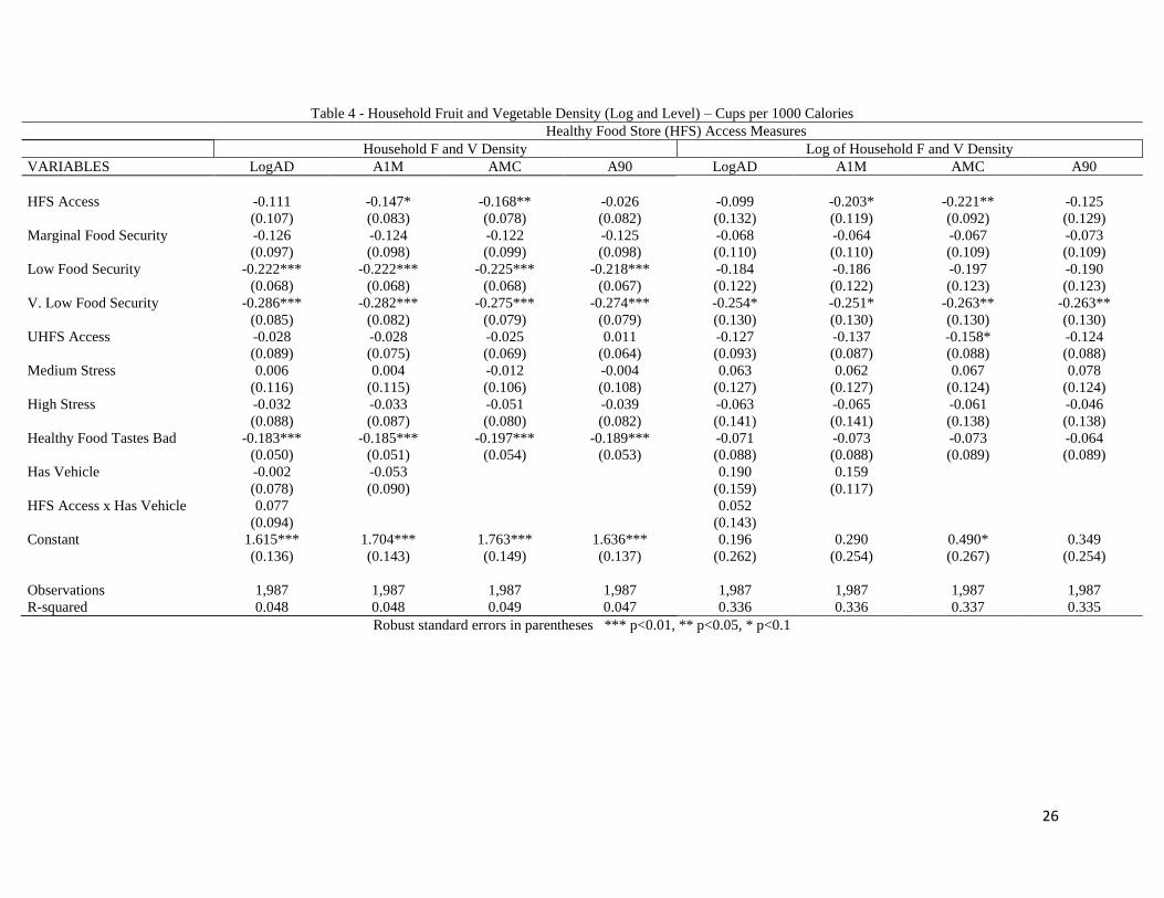
F-tests of the three food security indicators are highly significant (p<.05 or .01)
for all regressions except for the ones predicting log density. F-tests of low and very low
food security, without marginal security, produce the same level of significance or better
23
for the same dependent variables, and are consistently significant at predicting log
density (p<.10). Of the three dummies, low and very low food security have the largest
individual effects and are most consistently significant. Though their exact coefficients
vary somewhat between regressions, they are consistently negative and approximately the
same size across regressions with the same dependent variables. Compared to a
household with high food security, a household with very low food security would have
an HEI that is about 2.3 points lower, a fruit and vegetable ratio that is about 15.7
percentage points lower (level) or lower by about 42 percet (log ratio), and purchases .28
fewer cups of fruit and vegetables per 1000 Calories (density), which is about 23 percent
less (log density). The magnitude and robustness of these results indicates that food
insecurity has a strong association with households consuming less healthy food.
Disliking the taste of healthy food consistently predicts lower HEI, a lower fruit
and vegetable ratio (p<.01) and lower density (p<.01) for all regressions, but is
insignificant for regressions with logged dependent variables. This taste preference is
associated with a HEI that is about 2.1 points lower, a ratio about 9.2 percentage points
lower, and density that is about .185 cups per 1000 Calories lower. Meanwhile, the stress
indicators are jointly significant based on F tests (p<.01), but only for the ratio and log
ratio dependent variables. Compared to a household with low stress factors, a household
with a high number of factors is predicted to have a ratio which is about 17.2 points
lower, or 34 percent lower (log ratio). For these dependent variables, effect sizes are
robust between specifications. Finally, UHFS is only significant when predicting the log
ratio (p<.05), indicating that living within .5 miles of a greater than median number of
unhealthy food stores is associated with a fruit and vegetable ratio that is 25 percent
lower.
In summary, these results indicate that HFS access may be related to purchases,
but that this relationship, which is strongest for the access at median close measure, is not
entirely robust to how access is defined. It also appears that demand for healthy food is
distance inelastic, especially for households with cars. Meanwhile, food insecurity and
disliking the taste of healthy food robustly predict less healthy food purchases. The

24
effects of stress and UHFS proximity are mixed. However, the fact that significance
varies greatly between the log and level dependent variables is concerning.
Table 2 - Healthy Eating Index (or log)
Healthy Food Store (HFS) Access Measures
VARIABLES LogAD A1M AMC A90 LogHEI~LogAD
HFS Access -0.920 -0.702 -0.941 -0.123 0.002
(0.907) (0.773) (0.632) (0.831) (0.144)
Marginal Food Security -1.505* -1.498* -1.516* -1.534* -0.026
(0.831) (0.830) (0.830) (0.832) (0.114)
Low Food Security -2.136*** -2.127*** -2.189*** -2.149*** -0.009
(0.811) (0.810) (0.811) (0.809) (0.126)
V. Low Food Security -2.298** -2.258** -2.345*** -2.338*** -0.177
(0.914) (0.909) (0.905) (0.906) (0.143)
UHFS Access -0.647 -0.673 -0.845 -0.642 0.008
(0.664) (0.645) (0.629) (0.622) (0.097)
Medium Stress -0.287 -0.289 -0.221 -0.173 0.290**
(0.911) (0.912) (0.905) (0.904) (0.136)
High Stress -0.894 -0.896 -0.834 -0.766 0.223
(0.939) (0.940) (0.932) (0.931) (0.153)
Healthy Food Tastes Bad -2.124*** -2.143*** -2.116*** -2.069*** -0.089
(0.699) (0.699) (0.697) (0.695) (0.099)
Has Vehicle 1.673* 1.023 -0.034
(0.976) (0.738) (0.170)
HFS Access x Has Vehicle 0.974 0.058
(0.992) (0.157)
Constant 51.332*** 52.037*** 53.131*** 52.408*** 4.381***
(1.835) (1.804) (1.846) (1.764) (0.293)
Observations 1,987 1,987 1,987 1,987 1,987
R-squared 0.253 0.253 0.253 0.252 0.417
Robust standard errors in parentheses, note that column five is not a primary specification but is included to
determine distance elasticity of demand. *** p<0.01, ** p<0.05, * p<0.1

25
Table 3 - Household Fruit and Vegetable Ratio (level and log)
Healthy Food Store (HFS) Access Measures
Household F and V Ratio Log of Household F and V Ratio
VARIABLES LogAD A1M AMC A90 LogAD A1M AMC A90
HFS Access -6.927** -3.771 -6.601** -3.456 -0.496** -0.423** -0.397*** -0.519***
(3.184) (3.321) (2.600) (3.668) (0.199) (0.178) (0.138) (0.193)
Marginal Food Security -4.529 -4.492 -4.517 -4.687 0.015 0.023 0.019 0.003
(3.704) (3.711) (3.717) (3.714) (0.170) (0.169) (0.169) (0.169)
Low Food Security -13.775*** -13.682*** -14.007*** -13.799*** -0.373** -0.370** -0.384** -0.379**
(3.429) (3.436) (3.457) (3.448) (0.181) (0.181) (0.183) (0.182)
V. Low Food Security -15.795*** -15.480*** -15.768*** -15.782*** -0.547*** -0.525*** -0.537*** -0.544***
(3.506) (3.536) (3.569) (3.569) (0.201) (0.200) (0.201) (0.200)
UHFS Access -1.808 -1.702 -2.737 -1.702 -0.321** -0.277** -0.289** -0.274**
(3.121) (2.740) (2.782) (2.694) (0.141) (0.133) (0.134) (0.133)
Medium Stress -15.537*** -15.548*** -15.511*** -15.196*** 0.004 -0.001 -0.002 0.014
(4.461) (4.472) (4.441) (4.446) (0.202) (0.202) (0.199) (0.199)
High Stress -17.294*** -17.314*** -17.343*** -16.900*** -0.426* -0.429* -0.432** -0.407*
(4.307) (4.313) (4.276) (4.271) (0.221) (0.221) (0.219) (0.219)
Healthy Food Tastes Bad -9.144*** -9.262*** -9.353*** -9.097*** 0.031 0.025 0.020 0.025
(2.395) (2.403) (2.369) (2.358) (0.135) (0.136) (0.135) (0.135)
Has Vehicle 8.518** 3.449 0.457* 0.200
(3.806) (2.965) (0.238) (0.176)
HFS Access x Has Vehicle 7.469** 0.373*
(3.741) (0.218)
Constant 79.893*** 84.756*** 90.781*** 86.490*** 3.182*** 3.518*** 3.811*** 3.651***
(8.659) (8.488) (8.865) (8.498) (0.407) (0.394) (0.409) (0.396)
Observations 1,987 1,987 1,987 1,987 1,987 1,987 1,987 1,987
R-squared 0.061 0.060 0.062 0.059 0.214 0.213 0.213 0.213
Robust standard errors in parentheses *** p<0.01, ** p<0.05, * p<0.1
26
Table 4 - Household Fruit and Vegetable Density (Log and Level) – Cups per 1000 Calories
Healthy Food Store (HFS) Access Measures
Household F and V Density Log of Household F and V Density
VARIABLES LogAD A1M AMC A90 LogAD A1M AMC A90
HFS Access -0.111 -0.147* -0.168** -0.026 -0.099 -0.203* -0.221** -0.125
(0.107) (0.083) (0.078) (0.082) (0.132) (0.119) (0.092) (0.129)
Marginal Food Security -0.126 -0.124 -0.122 -0.125 -0.068 -0.064 -0.067 -0.073
(0.097) (0.098) (0.099) (0.098) (0.110) (0.110) (0.109) (0.109)
Low Food Security -0.222*** -0.222*** -0.225*** -0.218*** -0.184 -0.186 -0.197 -0.190
(0.068) (0.068) (0.068) (0.067) (0.122) (0.122) (0.123) (0.123)
V. Low Food Security -0.286*** -0.282*** -0.275*** -0.274*** -0.254* -0.251* -0.263** -0.263**
(0.085) (0.082) (0.079) (0.079) (0.130) (0.130) (0.130) (0.130)
UHFS Access -0.028 -0.028 -0.025 0.011 -0.127 -0.137 -0.158* -0.124
(0.089) (0.075) (0.069) (0.064) (0.093) (0.087) (0.088) (0.088)
Medium Stress 0.006 0.004 -0.012 -0.004 0.063 0.062 0.067 0.078
(0.116) (0.115) (0.106) (0.108) (0.127) (0.127) (0.124) (0.124)
High Stress -0.032 -0.033 -0.051 -0.039 -0.063 -0.065 -0.061 -0.046
(0.088) (0.087) (0.080) (0.082) (0.141) (0.141) (0.138) (0.138)
Healthy Food Tastes Bad -0.183*** -0.185*** -0.197*** -0.189*** -0.071 -0.073 -0.073 -0.064
(0.050) (0.051) (0.054) (0.053) (0.088) (0.088) (0.089) (0.089)
Has Vehicle -0.002 -0.053 0.190 0.159
(0.078) (0.090) (0.159) (0.117)
HFS Access x Has Vehicle 0.077 0.052
(0.094) (0.143)
Constant 1.615*** 1.704*** 1.763*** 1.636*** 0.196 0.290 0.490* 0.349
(0.136) (0.143) (0.149) (0.137) (0.262) (0.254) (0.267) (0.254)
Observations 1,987 1,987 1,987 1,987 1,987 1,987 1,987 1,987
R-squared 0.048 0.048 0.049 0.047 0.336 0.336 0.337 0.335
Robust standard errors in parentheses *** p<0.01, ** p<0.05, * p<0.1
27
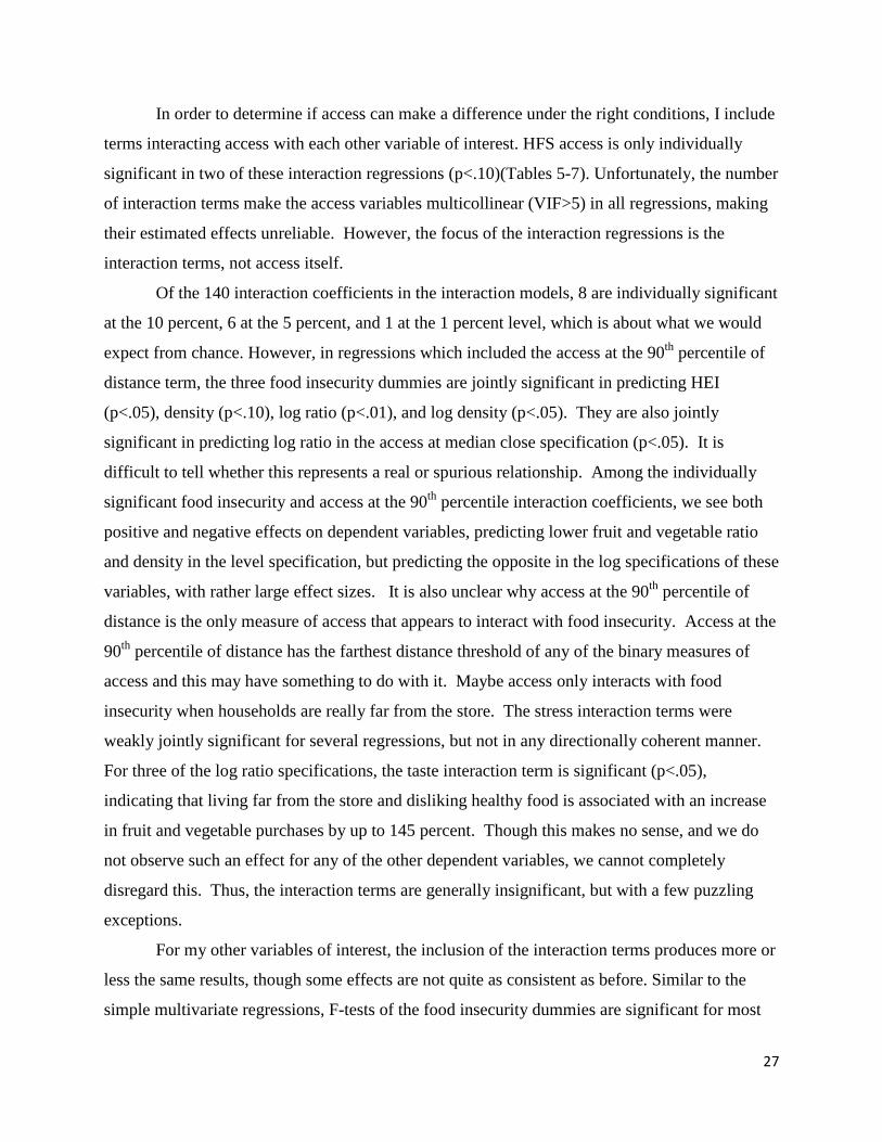
In order to determine if access can make a difference under the right conditions, I include
terms interacting access with each other variable of interest. HFS access is only individually
significant in two of these interaction regressions (p<.10)(Tables 5-7). Unfortunately, the number
of interaction terms make the access variables multicollinear (VIF>5) in all regressions, making
their estimated effects unreliable. However, the focus of the interaction regressions is the
interaction terms, not access itself.
Of the 140 interaction coefficients in the interaction models, 8 are individually significant
at the 10 percent, 6 at the 5 percent, and 1 at the 1 percent level, which is about what we would
expect from chance. However, in regressions which included the access at the 90th
percentile of
distance term, the three food insecurity dummies are jointly significant in predicting HEI
(p<.05), density (p<.10), log ratio (p<.01), and log density (p<.05). They are also jointly
significant in predicting log ratio in the access at median close specification (p<.05). It is
difficult to tell whether this represents a real or spurious relationship. Among the individually
significant food insecurity and access at the 90th
percentile interaction coefficients, we see both
positive and negative effects on dependent variables, predicting lower fruit and vegetable ratio
and density in the level specification, but predicting the opposite in the log specifications of these
variables, with rather large effect sizes. It is also unclear why access at the 90th
percentile of
distance is the only measure of access that appears to interact with food insecurity. Access at the
90th
percentile of distance has the farthest distance threshold of any of the binary measures of
access and this may have something to do with it. Maybe access only interacts with food
insecurity when households are really far from the store. The stress interaction terms were
weakly jointly significant for several regressions, but not in any directionally coherent manner.
For three of the log ratio specifications, the taste interaction term is significant (p<.05),
indicating that living far from the store and disliking healthy food is associated with an increase
in fruit and vegetable purchases by up to 145 percent. Though this makes no sense, and we do
not observe such an effect for any of the other dependent variables, we cannot completely
disregard this. Thus, the interaction terms are generally insignificant, but with a few puzzling
exceptions.
For my other variables of interest, the inclusion of the interaction terms produces more or
less the same results, though some effects are not quite as consistent as before. Similar to the
simple multivariate regressions, F-tests of the food insecurity dummies are significant for most

28
specifications, consistently predicting lower fruit and vegetable ratios (p<.01) and lower density
(p<.05 or .01) , but no longer predict the log of density, and no longer consistently predict HEI
and log ratio. In spite of this, the size and direction of the food insecurity coefficients are robust
to the inclusion of interaction terms. The coefficients for stress, UHFS proximity, and taste
preferences are also mostly consistent between the simple multivariate and interaction
regressions, both in their significances and in their effect sizes.
Table 5 - Healthy Eating Index – Interaction Regressions
Healthy Food Store (HFS) Access Measures
VARIABLES LogAD A1M AMC A90
Access (HFS) 0.319 0.937 -1.678 1.283
(1.161) (1.922) (1.802) (2.101)
Marginal Food Security -2.061** -1.380 -0.550 -1.094
(1.013) (0.947) (1.128) (0.899)
Low Food Security -2.822*** -1.721* -1.324 -1.686*
(0.993) (0.908) (1.029) (0.881)
V. Low Food Security -3.428*** -1.797* -1.941* -1.300
(1.135) (1.031) (1.175) (0.985)
UHFS Access -0.387 -0.768 -1.550* -0.885
(0.842) (0.696) (0.818) (0.671)
Medium Stress -0.263 0.045 -0.444 -0.333
(1.101) (1.050) (1.263) (1.004)
High Stress -0.508 -0.544 -1.413 -0.899
(1.136) (1.077) (1.298) (1.040)
Healthy Food Tastes Bad -1.975** -2.278*** -2.794*** -1.828**
(0.857) (0.780) (0.879) (0.755)
Has Vehicle 1.037 1.021
(0.736) (0.738)
Access x Marginal Food Security -1.083 -0.342 -2.184 -2.522
(1.136) (1.985) (1.658) (2.312)
Access x Low Food Security -1.261 -1.989 -2.420 -2.901
(1.091) (2.034) (1.633) (2.143)
Access x V. Low Food Security -1.999* -2.319 -1.182 -6.558***
(1.207) (2.182) (1.808) (2.364)
Access x UHFS Access 0.379 0.942 1.894 2.084
(0.900) (1.871) (1.267) (1.778)
Access x Medium Stress -0.094 -1.304 0.682 1.277
(1.179) (2.041) (1.791) (2.278)
Access x High Stress 0.580 -1.499 1.389 0.754
(1.224) (2.092) (1.828) (2.235)
Access x Healthy Food Tastes Bad 0.293 0.643 1.925 -1.927
(0.921) (1.779) (1.404) (1.881)
Constant 51.983*** 51.615*** 53.511*** 52.093***
(1.845) (1.885) (2.065) (1.816)
Observations 1,987 1,987 1,987 1,987
R-squared 0.254 0.254 0.255 0.256
Robust standard errors in parentheses
*** p<0.01, ** p<0.05, * p<0.1
29
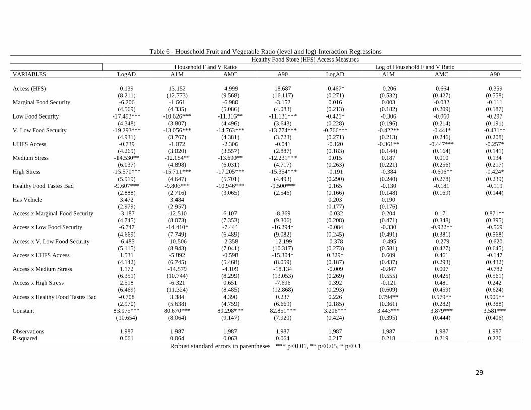
Table 6 - Household Fruit and Vegetable Ratio (level and log)-Interaction Regressions Healthy Food Store (HFS) Access Measures
Household F and V Ratio Log of Household F and V Ratio
VARIABLES LogAD A1M AMC A90 LogAD A1M AMC A90
Access (HFS) 0.139 13.152 -4.999 18.687 -0.467* -0.206 -0.664 -0.359
(8.211) (12.773) (9.568) (16.117) (0.271) (0.532) (0.427) (0.558)
Marginal Food Security -6.206 -1.661 -6.980 -3.152 0.016 0.003 -0.032 -0.111
(4.569) (4.335) (5.086) (4.083) (0.213) (0.182) (0.209) (0.187)
Low Food Security -17.493*** -10.626*** -11.316** -11.131*** -0.421* -0.306 -0.060 -0.297
(4.348) (3.807) (4.496) (3.643) (0.228) (0.196) (0.214) (0.191)
V. Low Food Security -19.293*** -13.056*** -14.763*** -13.774*** -0.766*** -0.422** -0.441* -0.431**
(4.931) (3.767) (4.381) (3.723) (0.271) (0.213) (0.246) (0.208)
UHFS Access -0.739 -1.072 -2.306 -0.041 -0.120 -0.361** -0.447*** -0.257*
(4.269) (3.020) (3.557) (2.887) (0.183) (0.144) (0.164) (0.141)
Medium Stress -14.530** -12.154** -13.690** -12.231*** 0.015 0.187 0.010 0.134
(6.037) (4.898) (6.031) (4.717) (0.263) (0.221) (0.256) (0.217)
High Stress -15.570*** -15.711*** -17.205*** -15.354*** -0.191 -0.384 -0.606** -0.424*
(5.919) (4.647) (5.701) (4.493) (0.290) (0.240) (0.278) (0.239)
Healthy Food Tastes Bad -9.607*** -9.803*** -10.946*** -9.500*** 0.165 -0.130 -0.181 -0.119
(2.888) (2.716) (3.065) (2.546) (0.166) (0.148) (0.169) (0.144)
Has Vehicle 3.472 3.484 0.203 0.190
(2.979) (2.957) (0.177) (0.176)
Access x Marginal Food Security -3.187 -12.510 6.107 -8.369 -0.032 0.204 0.171 0.871**
(4.745) (8.073) (7.353) (9.306) (0.208) (0.471) (0.348) (0.395)
Access x Low Food Security -6.747 -14.410* -7.441 -16.294* -0.084 -0.330 -0.922** -0.569
(4.669) (7.749) (6.489) (9.082) (0.245) (0.491) (0.381) (0.568)
Access x V. Low Food Security -6.485 -10.506 -2.358 -12.199 -0.378 -0.495 -0.279 -0.620
(5.115) (8.943) (7.041) (10.317) (0.273) (0.581) (0.427) (0.645)
Access x UHFS Access 1.531 -5.892 -0.598 -15.304* 0.329* 0.609 0.461 -0.147
(4.142) (6.745) (5.468) (8.059) (0.187) (0.437) (0.293) (0.432)
Access x Medium Stress 1.172 -14.579 -4.109 -18.134 -0.009 -0.847 0.007 -0.782
(6.351) (10.744) (8.299) (13.053) (0.269) (0.555) (0.425) (0.561)
Access x High Stress 2.518 -6.321 0.651 -7.696 0.392 -0.121 0.481 0.242
(6.469) (11.324) (8.485) (12.868) (0.293) (0.609) (0.459) (0.624)
Access x Healthy Food Tastes Bad -0.708 3.384 4.390 0.237 0.226 0.794** 0.579** 0.905**
(2.970) (5.638) (4.759) (6.669) (0.185) (0.361) (0.282) (0.388)
Constant 83.975*** 80.670*** 89.298*** 82.851*** 3.206*** 3.443*** 3.879*** 3.581***
(10.654) (8.064) (9.147) (7.920) (0.424) (0.395) (0.444) (0.406)
Observations 1,987 1,987 1,987 1,987 1,987 1,987 1,987 1,987
R-squared 0.061 0.064 0.063 0.064 0.217 0.218 0.219 0.220
Robust standard errors in parentheses *** p<0.01, ** p<0.05, * p<0.1

30
Table 7 - Household Fruit and Vegetable Density (Log and Level) – Cups per 1000 Calories – Interaction Regressions Healthy Food Store (HFS) Access Measures
Household F and V Density Log of Household F and V Density
VARIABLES LogAD A1M AMC A90 LogAD A1M AMC A90
Access (HFS) -0.003 -0.075 -0.151 0.131 -0.241 -0.217 -0.497* -0.188
(0.090) (0.161) (0.148) (0.179) (0.166) (0.320) (0.261) (0.336)
Marginal Food Security -0.170** -0.113 -0.066 -0.117 -0.067 -0.113 -0.041 -0.143
(0.080) (0.130) (0.178) (0.119) (0.140) (0.116) (0.135) (0.120)
Low Food Security -0.269*** -0.182** -0.185** -0.166** -0.141 -0.166 -0.067 -0.165
(0.082) (0.078) (0.091) (0.073) (0.155) (0.132) (0.145) (0.128)
V. Low Food Security -0.322*** -0.250*** -0.270*** -0.224*** -0.333* -0.231* -0.265 -0.201
(0.100) (0.092) (0.095) (0.081) (0.172) (0.140) (0.162) (0.135)
UHFS Access 0.008 -0.015 -0.054 0.010 -0.082 -0.131 -0.265** -0.126
(0.079) (0.091) (0.112) (0.074) (0.123) (0.094) (0.108) (0.092)
Medium Stress -0.031 0.025 0.019 0.007 0.114 0.113 -0.002 0.104
(0.113) (0.131) (0.154) (0.121) (0.163) (0.139) (0.161) (0.135)
High Stress -0.012 -0.073 -0.127 -0.062 0.141 -0.092 -0.263 -0.092
(0.098) (0.094) (0.101) (0.086) (0.183) (0.151) (0.173) (0.149)
Healthy Food Tastes Bad -0.201*** -0.178*** -0.172** -0.167*** -0.102 -0.125 -0.084 -0.097
(0.055) (0.059) (0.077) (0.058) (0.110) (0.097) (0.111) (0.096)
Has Vehicle -0.058 -0.050 0.155 0.159
(0.091) (0.092) (0.117) (0.117)
Access x Marginal Food Security -0.088 -0.050 -0.117 0.001 -0.001 0.239 -0.030 0.530*
(0.121) (0.207) (0.222) (0.216) (0.142) (0.313) (0.225) (0.272)
Access x Low Food Security -0.091 -0.202 -0.097 -0.334* 0.083 -0.136 -0.370 -0.178
(0.084) (0.155) (0.138) (0.175) (0.163) (0.340) (0.252) (0.397)
Access x V. Low Food Security -0.069 -0.133 -0.012 -0.314 -0.131 -0.064 -0.019 -0.369
(0.081) (0.151) (0.152) (0.199) (0.171) (0.364) (0.270) (0.412)
Access x UHFS Access 0.067 -0.122 0.046 -0.020 0.077 -0.066 0.273 0.002
(0.112) (0.160) (0.140) (0.172) (0.122) (0.305) (0.192) (0.312)
Access x Medium Stress -0.075 -0.091 -0.085 -0.085 0.090 -0.252 0.161 -0.215
(0.094) (0.151) (0.158) (0.175) (0.165) (0.335) (0.258) (0.351)
Access x High Stress 0.031 0.207 0.184 0.144 0.364** 0.157 0.490* 0.310
(0.082) (0.171) (0.135) (0.190) (0.180) (0.376) (0.282) (0.390)
Access x Healthy Food Tastes Bad -0.029 -0.002 -0.067 -0.180 -0.063 0.310 0.057 0.188
(0.068) (0.100) (0.103) (0.122) (0.119) (0.242) (0.185) (0.248)
Constant 1.683*** 1.677*** 1.762*** 1.599*** 0.118 0.270 0.601** 0.333
(0.145) (0.147) (0.163) (0.141) (0.270) (0.256) (0.288) (0.260)
Observations 1,987 1,987 1,987 1,987 1,987 1,987 1,987 1,987
R-squared 0.049 0.050 0.051 0.049 0.338 0.338 0.340 0.338
Robust standard errors in parentheses *** p<0.01, ** p<0.05, * p<0.1

31
In summary, the interaction regressions provide weak and puzzling evidence that food
insecurity and taste preferences may interact with access, indicating that the effect of being far
away from supermarkets may differ depending on other factors, but only under specific
circumstances. Though coefficients are less often significant than in the simple multivariate
regressions, the effects of the non-access variables of interest are generally robust to the
inclusion of interaction terms. This provides good evidence of the robustness of these factors in
predicting worse food purchases, indicating that other factors may matter more than access.
VI. Discussion and Limitations
The results for access are puzzling, showing inconsistent significance for the ratio and
density (and log) dependent variables, with access at median close being the most consistent. It
could be that this is because access at median close is the most valid of these measures.
However, though it incorporates household information about what counts as nearby, it does not
always do this well. For example, it counts one third of households that said their store was
nearby as lacking access, more than access at the 90th
percentile of distance or access at 1 mile.
In general, access at median close counts 40% of the sample as lacking access, far more than the
other binary measures. There are a few statistics to keep in mind when thinking about this.
Firstly, though some of the effects of access are significant, these effects are not very large
compared to other factors such as food insecurity or taste preferences. Secondly, descriptive
statistics support the idea that access does matter a little bit. Households without access (based
on access at median close and access at the 90th
percentile of distance) are less likely to have
gone shopping during the week observed, and are less likely to shop at a HFS (see Table 1),
though these differences are not very large. Additionally, households lacking access are much
less likely to have a vehicle, though this difference, and the previously mentioned differences, is
largest for access at the 90th
percentile of distance, which was the least significant of all the
access measures. In general, these findings indicate that food deserts may be associated with
differences in purchases, but it is not enough to reject my hypothesis that they do not.
It is worth mentioning the possibility of a relationship between access, frequency of
shopping, and purchases. The data shows that that households lacking access were less likely to
32
have gone shopping during the week of data collection, based on the median close and 90th
percentile of distance measures of access. Though this estimated difference, at its largest, only
accounts for 5% of the households in food deserts, the true differences in frequency of shopping
may be larger. This is because households in my sample are defined as having gone shopping if
they obtained more than zero items for consumption at home. This is guaranteed to over count
the households who actually went grocery shopping, given that a household that bought one
candy bar would count as having done a full shopping trip. However, if households in food
deserts do shop less frequently in response to having to travel farther to the store, then this might
impact their purchases. If the time in between shopping trips were long enough for fruits and
vegetables to spoil before a household had the chance to eat them, then such a household
probably would not buy as much produce as a household that shopped every week. Instead, they
might only buy an amount that they could finish before it went bad, even if that meant going
days or weeks without fresh fruits and vegetables. This effect would also likely depend on a
household’s access to refrigerated storage, which likely depends on income. In this way, food
deserts could potentially affect diet by affecting the timing of shopping trips, and future research
should keep this in mind.
Also related to timing is the distribution of SNAP benefits. Evidence suggests that many
households receiving SNAP spend all or most of these benefits as soon as they are received
(Widener and Shannon 2014). This likely affects the general timing of recipient’s grocery trips,
possibly causing them to shop less frequently. If this, in turn, affects which foods people
purchase, and especially if this depends on other factors such as access, then my SNAP control
variable may not sufficiently account for confounding variation caused by benefit timing. It
does, however, indicate that timing of benefits might make a good future instrumental variable
for the decision to go shopping in any given week among SNAP households.
Results for stress were generally week. Stress consistently predicts the ratio and log ratio
measures, but not other measures of fruit and vegetable consumption or HEI, though it is unclear
why. This is likely because my measure of stress was flawed in several ways, though it is still a
good first step to examining the relationship between stress and food deserts. Particularly, my
variable conflates stress with being too busy to make healthy food, which is not the same thing,
even though they may both have similar effects on diet. I conceptualize stress as something that

33
breaks down people’s willpower to adhere to a healthy diet and tempts them into eating junk
food, whereas lacking time, while possibly causing stress, can be thought of as a hard logistical
barrier to preparing food which may have a distinct impact. Given that the FoodAPS data does
not include a direct measure of stress, I constructed the stress variable based on anything in the
data that might be associated with stress, many of which, such as employment and childrearing,
may also be associated with having limited time. For this reason, my stress variable may not be a
very appropriate estimator for what it seeks to measure. This may be why the effects of stress
were weakly consistent in my results.
My strongest results are for food insecurity and taste preferences. Given their fairly
consistent significance, consistent effect sizes, and the robustness of these to the inclusion of
interaction terms, this provides good evidence for my hypothesis that there is a real association
between these variables and lower purchases of fruits and vegetables and worse overall market
basket quality. This could mean that people who cannot afford enough food economize by
buying less fruits and vegetables, and that people who dislike the taste of healthy food eat less of
it, or these associations could be due to some unobserved factors. Whatever the nature of this
relationship, there is limited evidence that these factors may interact with HFS access under
specific circumstances. However, my results indicate that access does not interact significantly
with other dependent variables most of the time. This may mean that the effects of access do not
differ depending on circumstances such as stress, but there is also number of potential problems
with my results.
Another problem is that the regressions predicting the logged dependent variables differ
greatly from their level specifications. For example, in the simple multivariate regressions, all
measures of access are significant in specifications predicting log ratio, unlike every other
dependent variables. It cannot be that access simultaneously does and does not affect total fruit
and vegetable purchases, so at least one measure of this dependent variable must be causing bias.
One possible explanation for this is that the logged variables might not be a very appropriate
measure of food purchases. Neither log ratio nor log density are entirely normally distributed
(Appendix C), and this could systematically bias coefficient estimates in ways that are hard to
predict. This may be why the results differed between log and level specifications. Alternately, it
could be that the logged variables are good measures of purchases, and it is the unlogged
34
versions, with their strong right skew, which create bias. At this point, it is indeterminate which
of these scenarios more accurately describes these results.
Inability to control for food waste could also bias my results. Given that it goes bad
pretty quickly, produce probably has a high rate of food waste, and thus my estimates of fruit and
vegetable consumption may overstate how much is actually being eaten. This means that any
effect that my variables have on purchases would overstate the effect on actual diet, which means
all my coefficients are probably biased downward, away from zero. It would also be a problem
if the level of food waste differs depending on one of my variables of interest, such as food
insecurity. If, for example, food secure households waste more fruit than food insecure
households, then fruit purchases would overstate fruit intake for one group but not the other.
This could cause my regressions to overstate the extent to which food insecurity reduced fruit
intake, further biasing my food security coefficients downward.
Another problem is that my estimates of weekly recommended fruit and vegetable
consumption, used in my ratio dependent variables, are based on the assumption that everyone is
moderately physically active. However, not everyone is moderately physically active and it is
likely level of physical activity varies systematically with food insecurity, stress, and potentially
other factors as well. If stressed people deal with their stress by exercising then their dietary
recommendations would be too small, making an inadequate amount of fruit look sufficient.
This could cause upward bias in the estimated effect of high stress on food purchases, potentially
making it look like stress does not decrease market basket quality as much as it really does. If,
on the other hand, lacking sufficient nutrients makes food insecure people less willing to burn
energy exercising, then my estimate of their recommended dietary intake would be too large,
deflating their apparent purchases to dietary recommendation ratio. This would cause upward
bias on my coefficient for food insecurity, causing the model to understate the detrimental
impact of food insecurity on food quality.
There are other potential problems with the data whose effects are hard to predict. A
major potential drawback of the FoodAPS data is that having to keep track of food for a week
changes some aspect of how people spend money on food or what food they buy, and thus the
act of observing might change the observation. I have no way of knowing if this would cause
people to eat better or worse or put off shopping all together and no way of knowing if this effect

35
is correlated with my variables of interest. Similarly, the kind of people who agree to participate
in such a survey may systematically differ, in some unknown way, from the kind of people who
do not. Either of these could damage the validity of the data, and thus any results based on it.
What is more, even in the unlikely event that my controls successfully removed all
endogeneity, there are still a number of potential threats to the validity and applicability of my
findings. The results of this study are general. We should keep in mind that there may be some
subgroup of the LI-LA population for whom the results do not hold.
VII. Conclusion
To conclude, this paper investigates the relative impacts of geographic proximity to
healthy food stores, overexposure to unhealthy food stores, food insecurity, preferences, and
stress factors on the foods purchased or otherwise obtained by low income, non-rural
households. I found that household food insecurity is strongly associated with lower fruit and
vegetable purchases and lower overall market basket quality. Similarly, when members of a
household think that healthy food tastes bad, then they are less likely to purchase it. Meanwhile,
having a medium or high number of stress factors, as opposed to a small number, is associated
with obtaining fewer fruits and vegetables, but only for some measures of consumption.
Living near a large number of fast food restaurants and convenience stores had a weak
effect. However, living without access to a healthy food store, or living farther from the nearest
healthy food store, is somewhat consistently associated with lower fruit and vegetable purchases.
These effects are not large, but neither are they inconsequentially small. In general though,
purchases appeared to be distance inelastic, and the effects of access, when defined solely as
distance, appear to be present only for households without a private vehicle. Access might
interact with food insecurity and taste preferences, but these interactions are not robust. In
general, most households in the sample primarily shopped at healthy food stores and went
shopping during the data observation period, and households in food deserts were somewhat less
likely to do both of these things. Additionally, though most households did have vehicles,
households without access were much less likely to. Based on these results, it appears that access
to healthy food stores has a questionable effect on people’s food consumption, but that food
36
insecurity and dislike of healthy foods do have a much stronger association with consuming less
healthy food, and this has potential implications for diet.
To clarify the importance of food deserts, more research needs to be done to definitively
determine if there is a causal impact of store proximity on diet. This might involve doing
additional quasi experimental studies examining how the placement of supermarkets by retail
location programs affects diets in the recipient neighborhoods. Preferably this would be done by
comparing large samples of households in a large number of neighborhoods in multiple states
over a longer period of time. Without such research, it is hard to definitively say that living far
from healthy food retailers does not have any impact on diet. More research also needs to be
done to explore the potential interactions between food deserts and other factors. Specifically,
research should examine whether food deserts have an impact in conjunction with demographic
factors. So as to avoid multicollinearity, rather than doing an interaction approach as I did, it
might be worthwhile to predict food purchases in subsets defined by their access status, and to
compare the impacts of various demographic variables between these subsets.
There are also several modifications that future research could make to improve on the
present study. Firstly, researchers should consider, and investigate, the relationship between
food deserts and the frequency of shopping trips, as access could potentially affect diet by
affecting timing. When doing this, it may be useful to use the timing of SNAP benefits as a
source of exogenous variation in when people go shopping, especially when working with
datasets collected for a short period of time, such as Food APS. Additionally, researchers
interested in examining the effects of stress in the context of food environment should find a
better way to measure stress than simply tallying up a household’s total number of miscellaneous
stress factors, and should ensure that they do not conflate stress with time constraints.
Though there are certainly some individuals who do not buy healthy food because they
cannot get to the store, the question of this paper is whether we should shift our focus from food
environment to other factors such as food insecurity. Making useful public policy depends on
accurately assessing which factors contribute to a problem, and by how much. My results do not
provide conclusive enough evidence to rule out food deserts as impacting diet, but they also fail
to demonstrate a robust association. There is some inconsistent evidence to suggest that stress
may be related to diet, but my specification of stress is flawed in several ways, making this

37
finding unreliable. However, it is clear that food insecurity and taste preferences do appear to be
related to purchases, and these relationships appear to be large. Though a large amount of
research exists on food insecurity, my findings indicate that more research needs to be done
examining the role of taste preferences in shaping the diets of low income populations.
Additionally, in order to assess what policy makers should be focusing on, there needs to
be more cost benefit analysis of healthy food interventions. Future research should begin by
evaluating the relative merits of retail location programs like the Heathy Food Financing
Initiative compared to transfer and incentive programs such as the Healthy Incentives Pilot (HIP)
Program. HIP was a randomly controlled trial which gave treated SNAP participants the
purchasing power and incentives to consume healthier foods by providing them with an
immediate 30% rebate on any benefits spent on fruits and vegetables. This was found to be
successful at improving diet, causing a 5 point increase in households’ Healthy Eating Indexes
(Bartlett et al. 2014). In contrast, retail location programs have not been shown to have any
causal impact on diet, and it is unclear whether food deserts are even correlated with purchases.
The results presented in this paper indicate that any such relationship is not large. Furthermore,
the HIP is likely more scalable as a policy intervention than directing the location of
supermarkets nationwide. Because of this, even if food deserts do cause worse diets, it might be
more worthwhile to focus on other causes of unhealthy eating. Regardless of access or
demographic group, Americans are eating too much junk food and not enough fruits and
vegetables (Lee-Kwan et al. 2017), indicating that the problem extends beyond some subset of
urban neighborhoods.
However, it should also be acknowledged that though the effects of food deserts on diet
are questionable, they probably have other impacts. Experience of greater travel time and
difficulty of access are real burdens in and of themselves, regardless of whether they affect diet.
Though this paper is not focused on these costs, it is valid to consider food deserts to be a
problem simply because they are a nuisance.
It is my hope that the present study contributes useful information to the discussion of
food deserts and food access, and that this will help address the problems of ill dietary health in
low income communities. In addition to my findings, I contribute new approaches to assessing
the impact of access, both by using new measures of access, and by directing focus to the context

38
in which access may matter. Though my findings are not conclusive, I hope my approach will
inform the direction of future research.
Works Cited
Andreyeva, T., Blumenthal, D.M., Schwartz, M.B., Long, M.W., Brownell, K.D. (2008), Availability And Prices Of
Foods Across Stores And Neighborhoods: The Case Of New Haven, Connecticut, Health Affairs 27, no.5
(2008):1381-1388
Bartlett, S., Klerman, Olsho, L. et al. (2014) Evaluation of the Healthy Incentives Pilot (HIP): Final Report.
Prepared by Abt Associates for the U.S. Department of Agriculture, Food and Nutrition Service, September
2014.
Baumeister, R. F., Bratslavsky, E., Muraven, M., & Tice, D. M. (1998). Ego depletion: Is the active self a limited
resource? Journal of Personality and Social Psychology, 74(5), 1252-1265. http://dx.doi.org/10.1037/0022-
3514.74.5.1252
Bitler, M., Haider, S.J. (2011), An Economic View of Food Deserts in the United States, Journal of Policy Analysis
and Management, Vol. 30, No. 1, 153–176
Block JP1, Christakis NA, O'Malley AJ, Subramanian SV. (2011) Proximity to food establishments and body mass
index in the Framingham Heart Study offspring cohort over 30 years. Am J Epidemiol. 2011 Nov
15;174(10):1108-14. doi: 10.1093/aje/kwr244. Epub 2011 Sep 30.
Bodor, J. N., Rose, D., Farley, T. A., Swalm, C., and Scott, S. K. “Neighbourhood Fruit and Vegetable Availability
and Consumption: The Role of Small Food Stores in an Urban Environment.” Public Health Nutrition 11
(2007): 413-420
Broda, C., Leibtag, E., Weinstein, D.E. (2009) The Role of Prices in Measuring the Poor's Living Standards, The
Journal of Economic Perspectives, Vol. 23, No. 2 (Spring, 2009), pp. 77-97
Centers For Diesease Control, State Initiatives Supporting Healthier Food Retail: An Overview of the National
Landscape. https://www.cdc.gov/obesity/downloads/healthier_food_retail.pdf
Chung, C., Myers, S.L. Jr. (1999) Do the Poor Pay More for Food? An Analysis of Grocery Store Availability and
Food Price Disparities, The Journal of Consumer Affairs, Vol. 33, No. 2 (Winter 1999), pp. 276-296
Cummins S., A. Findlay, M. Petticrew, and L. Sparks (2005). “Healthy Cities: The Impact of Food Retail-led
Regeneration on Food Access, Choice and Retail Structure,” Built Environ 31(4): 288-301
Cummins,S., Flint, E., and Matthews, S. (2014) New Neighborhood Grocery Store Increased Awareness Of Food
Access But Did Not Alter Dietary Habits Or Obesity. HEALTH AFFAIRS 33,NO. 2 (2014): 283–291, doi:
10.1377/hlthaff.2013.0512
Currie, J., S. DellaVigna, E. Moretti, and V. Pathania (2009). “The Effect of Fast Food Restaurants on Obesity,”
National Bureau of Economic Research Working Paper No. 14721, http://www.nber.org/papers/w14721
Drewnowski A, Aggarwal A, Hurvitz PM, Monsivais P, Moudon AV. (2012) Obesity and supermarket access:
proximity or price? Am J Public Health 2012;102(8):e74–e80.
Dubowitz, Tamara, Madhumita Ghosh-Dastidar, Deborah A. Cohen, Robin Beckman, Elizabeth D. Steiner, Gerald
P. Hunter, Karen R. Florez, Christina Huang, Christine A., Vaughan, Jennifer C. Sloan, Shannon N. Zenk,
Steven Cummins, and Rebecca L. Collins. “Diet And Perceptions Change With Supermarket Introduction
in a Food Desert, But Not Because of Supermarket Use.” Health Affairs, (2015) 34:11:1858–1868.
Dubowitz T, Ghosh-Dastidar M, Eibner C, et al. The Women’s Health Initiative: the food environment,
neighborhood socioeconomic status, BMI, and blood pressure. Obesity (Silver Spring) 2012;20(4):862–71.
Elbel,,B., Moran, A., Dixon, B., Kiszko, K., Cantor, J., Abrams, C., Mijanovich, T. (2015) Assessment of a
government-subsidized supermarket in a high-need area on household food availability and children’s
dietary intakes. Public Health Nutrition: 18(15), 2881–2890 doi:10.1017/S1368980015000282
Ghosh-Dastidar, B., Cohen, D., Hunter, G., Zenk, S., Huang, C., Beckman, R., Dubowitz, T. (2012) Distance to
Store, Food Prices, and Obesity in Urban Food Deserts. American Journal of Preventative Medicine
2014;47(5):587–595
Glanz, K., Sallis, J.F., Saelens, B.E., Frank, L.D. (2007) Nutrition Environment Measures Survey in Stores (NEMS-
S) Development and Evaluation, American Journal of Preventive Medicine, 32(4):282–289)

39
Hagger, M. S., Wood, C., Stiff, C., & Chatzisarantis, N. L. D. (2010). Ego depletion and the strength model of self-
control: A meta-analysis. Psychological Bulletin, 136(4), 495-525. http://dx.doi.org/10.1037/a0019486
Handbury, J., Rahkovsky, I., Schnell, M. (2015) What drives nutritional disparities? Retail access and food
purchases across the socioeconomic spectrum. working paper
Hendrickson, D., Smith, C., and Eikenberry, N. (2004) Fruit and vegetable access in four low-income food deserts
communities in Minnesota, Agriculture and Human Values (2006) 23:371–383
Hofmann, Wilhelm & Rauch, Wolfgang & Gawronski, Bertram. (2007). And deplete us not into temptation:
Automatic attitudes, dietary restraint, and self-regulatory resources as determinants of eating behavior.
Journal of Experimental Social Psychology. 43. 497-504. 10.1016/j.jesp.2006.05.004.
Kahneman, D. (2011). Thinking, fast and slow. New York: Farrar, Straus and Giroux.
Kaushal, N. (2007) Do Food Stamps Cause Obesity? Evidence From Immigrant Experience. Journal of
Health Economics. 2007 Sep 1;26(5):968-91. Epub 2007 Feb 9
Kwate, N.O., Yau, C.Y., Loh, J.M., Williams, D. (2009) Inequality in obesogenic environments: Fast food density
in New York City, Health & Place 15, 364–373.
Kwate, N.O (2008) Fried chicken and fresh apples: Racial segregation as a fundamental cause of fast food density in
black neighborhoods, Health & Place 14 (2008) 32–44
Lee-Kwan SH, Moore LV, Blanck HM, Harris DM, Galuska D. (2017) Disparities in State-Specific Adult Fruit and
Vegetable Consumption — United States, 2015. MMWR Morb Mortal Wkly Rep 2017;66:1241–1247.
Leung, C., Willett, W., Ding, E.(2012) Low-income Supplemental Nutrition Assistance Program participation is
related to adiposity and metabolic risk factors. American Journal of Clinical Nutrition 2012;95:17–24.
Leung, C., Tester, J., Rimm, E., Willet, W. (2017) SNAP Participation and Diet-Sensitive Cardiometabolic Risk
Factors in Adolescents. American Journal of Preventative Medicine. 2017;52(2S2):S127–S137
Lin, BH., Morrison, R. (2014) ERS’s Food Consumption and Nutrient Intake Data—Tools for Assessing
Americans’ Diets, https://www.ers.usda.gov/amber-waves/2014/october/erss-food-consumption-and-
nutrient-intake-data-tools-for-assessing-americans-diets/
Monsivais, P., Aggarwal, A., Drewnowski, A.(2012) Are socio-economic disparities in diet quality explained by diet
cost?, Journal of Epidemiology and Community Health, Vol. 66, No. 6, pp. 530-535
Morland, K., Diex Roux, A., and Wing, S. “Supermarkets, Other Food Stores, and Obesity: The Atherosclerosis
Risk in Communities Study.” American Journal of Preventive Medicine 30, no.4 (2006): 333-339.
Muraven, M., & Baumeister, R. F. (2000). Self-regulation and depletion of limited resources: Does self-control
resemble a muscle? Psychological Bulletin, 126(2), 247-259. http://dx.doi.org/10.1037/0033-
2909.126.2.247
Office of Community Services (2017) Healthy Food Financing Initiative,
https://www.acf.hhs.gov/ocs/programs/community-economic-development/healthy-food-financing
Powell, L., Auld, C., Chaloupka, F., O’Malley, P. M., and Johnston, L. D. “Associations Between Access to Food
Stores and Adolescent Body Mass Index,” American Journal of Preventive Medicine 33, no.4 (2007).
Powell, L.M., Slater, S., Mirtcheva, D., Bao, Y., Chaloupka, F.J. (2007) Food store availability and neighborhood
characteristics in the United States, Preventive Medicine 44 189–195.
Rahkovsky, Ilya and Samantha Snyder. Food Choices and Store Proximity. ERR-195, U.S. Department of
Agriculture Economic Research Service, September 2015.
Rose, D., Bodor, N., Swalm, C., Rice, J., Farley, T., Hutchinson, P. (2009) Deserts in New Orleans? Illustrations of
Urban Food Access and Implications for Policy, working paper
Rose, D., and Richards, R. “Food Store Access and Household Fruit and Vegetable Use among Participants in the
US Food Stamp Program.” Public Health Nutrition 7, no.8 (2004):1081-1088.
Rundle, A., Neckerman, K., Freeman, L., Lovasi, G., Purciel, M., Quinn, J., Richards, C., Sircar, N., and Weiss, C.
“Neighborhood Food Environment and Walkability Predict Obesity in New York City.” Environmental
Health Perspectives 117 (2009): 442–447.
Shah, A., Mullainathan, S., Shafir, E. (2012) Some Consequences of Having Too Little, Science 02 Nov 2012:Vol.
338, Issue 6107, pp. 682-685 DOI: 10.1126/science.1222426
Stark JH, Neckerman K, Lovasi G, Konty K, Quinn J, Arno P, et al. Neighbourhood food environments and body
mass index among New York City adults. J Epidemiol Community Health. 2013;67(9):736–42.
Sturm, R., and Datar, A. “Body Mass Index in Elementary School Children, Metropolitan Area Food Prices and
Food Outlet Density.” Journal of Public Health 119 (2005):1059–1068.

40
The Reinvestment Fund (2011) Pennsylvania Fresh Food Financing Initiative, http://consumerfed.org/wp-
content/uploads/2011/10/Evans_Food_Deserts_panel_FPC_2011.pdf
Thomsen, M.R., Nayga, R.M. Jr., Alviola, P.A. IV, Rouse, H.L. (January, 2016) The Effect of Food Deserts On The
Body Mass Index of Elementary School Children, The American Journal of Agricultural Economics, 98(1):
1–18
U.S. Department of Agriculture and U.S. Department of Health and Human Services. Dietary Guidelines for
Americans, 2010. 7th Edition, Washington, DC: U.S. Government Printing Office, December 2010.
U.S. Department of Agricultrue (To be published late December 2017 or early 2018) USDA’s FoodAPS:
Methodology for Imputing Missing Quantities To Calculate HEI-2010 Scores and Sorting Foods into ERS
food groups.
Ver Ploeg, Michele, Lisa Mancino, Jessica E. Todd, Dawn Marie Clay, and Benjamin Scharadin. Where Do
Americans Usually Shop for Food and How Do They Travel To Get There? Initial Findings From the
National Household Food Acquisition and Purchase Survey. EIB-138, U.S. Department of Agriculture
Economic Research Service, March 2015.
Walker, Renee, E., Keane, Christopher, R., Burke, Jessica, G. (2010) Disparities and access to healthy food in the
United States: A review of food deserts literature, Health & Place, 16, 876–884.
Wang, M., Kim, S., Gonzalez, A., MacLeod, K., and Winkleby, M. “Socioeconomic and Food-Related Physical
Characteristics of the Neighborhood Environment are Associated with Body Mass Index.”Journal of
Epidemiology and Community Health 61 (2007): 491–498.
Weatherspoon,D, Oehmke, J., Dembe´le’, A., Coleman, M., Satimanon, T., Weatherspoon, L. (2013) Price and
Expenditure Elasticities for Fresh Fruits in an Urban Food Desert, Urban Studies, 50(1) 88–106
Widener, M.J., Shannon, J. (2014) When are food deserts? Integrating time into research on food accessibility,
Health & Place 30 (2014) 1–3

41
Appendix A
Figure 1
Figure 2

42
Appendix B: Explanation of Variables
Distance to nearest HFS (miles) – Distance to the nearest supermarket or superstore
Healthy Eating Index (HEI) – Measure of overall market basket quality derived by the USDA
HH Fruit and Veg Ratio – Ratio of household fruit and vegetable purchases for the week to recommended dietary
consumption for the week.
Cups of F and V per 1000 calories - Fruit and vegetable purchases, measured in cups, per 1000 calories
Income as % of Poverty Line – Household income as % of the poverty line for a household of that composition
Household w. Child Under 18 – Household has a child younger than 18
Shop at a HFS - Household shops at a supermarket or superstore
Low or V. Low Food Secure - Household has low or very low food security based on the USDA’Adult Food
Security Category measure.
UHFS Access – The number of convenience stores and fast food restaurants within half a mile of the household is
above the median number for the sample.
High Stress Factors – Household has a high number of stress factors, meaning it has more than one stress factor, or
more than one stress factor in addition to having a small child. See methods section.
Dislike Healthy Food – Primary Respondent said that members of the household think that healthy food tastes bad
Prim. Respondent Black – Primary respondent was black, this is included as a dummy in all primary regressions.
Prim. Respondent White - Primary respondent was white, this is included as a dummy in all primary regressions.4
Prim. Respondent Asian – Primary respondent is Asian American, Hawaiian native, or other pacific islander.
Prim. Respondent Other Race – Primary respondent was some other race
Prim. Respondent Hispanic – Primary respondent identified as Hispanic. This category is ethnic rather than racial
so it overlaps with all racial categories. This is included as a dummy in all primary regressions.
Did not go shopping – Did not obtain any food to be eaten at home during the data collection week
Did not go out to eat – Did not obtain any food to be eaten away from home during the data collection week
SNAP Recipient – Some member of the household was receiving SNAP benefits
Used Food Bank in Past Month – Household used food bank or food pantry to get groceries in the past 30 days
Owns or Leases a Vehicle – Household owns or leases a private vehicle
College Educated – Most educated household member had a bachelor’s degree or higher
High school Dropout – Most educated household member was a high school dropout
4 The omitted racial category for all regression consisted of all primary respondents who were Asian, multiple
races, some other race, or American Indian or Alaska Native

43
Appendix C: Distribution of Dependent Variables

44

45

46

47
Appendix D: Why Dropping Households that Did Not Go Shopping Would
Cause Bias
Dropping households that did not go shopping from my sample would bias my estimates.
Suppose you have 2 households of a particular population, and you want to know the average amount of
groceries that that population buys each week, but each household only goes shopping every other week,
and thus buys two weeks of groceries in that one trip. On any given week, say one bought 2 weeks’
worth of groceries that week and the other bought 0 groceries because it was their off week. If we take
the mean, we get the correct average amount of groceries that each household consumes each week,
which is to say, one weeks’ worth of groceries. If, on the other hand, you drop the household who did not
buy groceries that week and take the mean of the remaining population, then the only household
remaining is the one that bought enough for two weeks. Thus the average weekly grocery consumption of
the remaining household in the sample is 2 weeks’ worth of groceries, far more than it actually consumes.
Thus, excluding the household that did not go shopping that week from the sample creates upward bias in
our estimated mean grocery consumption. Now imagine we are comparing the means of two
populations. Imagine one population goes shopping every week, and the other goes shopping every other
week, possibly because they live in a food desert. If, in any given week, we drop households that did not
go shopping that week, then we will bias the estimated mean grocery purchases for one population but not
the other, and thus any seeming similarities or differences in this population’s grocery purchases would be
biased. Thus, my sample includes 213 households that did not obtain food to be eaten at home, and 58
households that did not obtain any food of any kind.

48
Appendix E: Why Controlling for Not Having Gone Shopping Sometimes
Causes Bias
Consider a world in which food deserts have no effect at all on the amount of healthy food a
person eats. Now imagine that to deal with longer travel time, people living in food deserts shopped less
frequently, but bought larger quantities of food to last them the weeks in between trips, while households
not in food deserts shop once a week and buy one week’s worth of food each trip. Say that we have
observed only a single one week period, and only know about shopping behavior, not what people
actually eat. If we predict household healthy food consumption based on food desert residency then we
would probably observe no relationship. However, things are different if we controlled for whether or not
someone shopped in the week observed. If we added this control then the coefficient on food desert
residence means the following: among households that did go shopping this week, this is how much more
households from food deserts bought. This means that, because people from food deserts bought more on
each trip, it will appear as though food deserts predict larger consumption of healthy food. Thus, if food
deserts have no effect, then controlling for shopping will create upwards bias in its coefficient, and
creating an effect size that is larger than it really is.
Now consider a world in which food deserts do matter, and reduce the healthy food consumption
of their residents. Imagine that food desert residents still shop less frequently and buy larger amounts of
food with each trip. Under this scenario, predictions of healthy food purchases will show that food
deserts reduce purchases, but estimates of this effect will not be very precise and we would expect large
errors. If we control for whether a household shopped that week, then the coefficient for food deserts will
still have the same interpretation as in the scenario above. It will compare the amount purchased by
people from food deserts with the amount purchased by everyone else, without accounting for how many
weeks those supplies are supposed to last for. This makes it appear as though food desert residents who
went shopping are eating more healthy food per week than they actually are. Thus, if food deserts do
decrease healthy food consumption then controlling for shopping will create upwards bias, resulting in a
smaller effect size which is likely more precise but less accurate. However, it is worth mentioning that, if
we do not control for access, the households not going shopping will create a lot of unexplained variation
within each category of access, likely making any real effects less statistically significant.
However, because they do not measure the amount of food bought, but rather the composition of
the food that is bought, these concerns do not apply to HEI and fruit and vegetable density. If, for
example, the HEIs of food desert residents and non-residents were the same, but their shopping patterns

49
different, then going shopping less frequently would make food desert residents appear to have a lower
average HEI because more households would have an HEI of 0. However, if you control for shopping,
then the coefficient on access would indicate the average effect of living in a food desert, among people
with the same shopping status, and thus this effect would be 0. This differs from if you are predicting the
quantities of fruits and vegetables purchased, where controlling for shopping makes it look as if food
desert residents were buying more of these items than they actually are, simply because they shop less
often. This difference exists because HEI is standardized by the total amount of food purchased, while
fruit and vegetable consumption is just a quantity (without regard for the total amount of other foods
purchased).
Now imagine that food desert residents still go shopping less often, but that they have lower HEI
in their actual diets than non-residents. In the absence of a control, the coefficient on food desert
residence might indicate some of this relationship, but the error would likely be large, meaning that this
effect might be insignificant. However, if we control for shopping then, unlike with quantities of food
purchased, it makes the error smaller because we are not trying to predict differences better explained by
other factors.

50
Appendix F: Food Insecurity Questionnaire
Top Related