


Languages
Pages
Legal


Factor Models for Asset Returns
Prof. Daniel P. PalomarThe Hong Kong University of Science and Technology (HKUST)
MAFS5310 - Portfolio Optimization with RMSc in Financial Mathematics
Fall 2020-21, HKUST, Hong Kong
Outline
1 Introduction
2 Linear Factor Models
3 Macroeconomic Factor Models
4 Fundamental Factor Models
5 Statistical Factor Models

Outline
1 Introduction
2 Linear Factor Models
3 Macroeconomic Factor Models
4 Fundamental Factor Models
5 Statistical Factor Models

Why Factor Models?
To decompose risk and return into explainable and unexplainable components.Generate estimates of abnormal returns.Describe the covariance structure of returns
without factors: the covariance matrix for N stocks requires N(N + 1)/2 parameters (e.g.,500(500 + 1)/2 = 125, 250)with K factors: the covariance matrix for N stocks requires N (K + 1) parameters withK � N (e.g., 500(3 + 1) = 2, 000)
Predict returns in specified stress scenarios.Provide a framework for portfolio risk analysis.
D. Palomar Factor Models 4 / 36

Types of Factor Models
Factor models decompose the asset returns into two parts: low-dimensional factors andidiosynchratic residual noise.1
Three types:1 Macroeconomic factor models
factors are observable economic and financial time seriesno systematic approach to choose factors
2 Fundamental factor modelsfactors are created from observable asset characteristicsno systematic approach to define the characteristics
3 Statistical factor modelsfactors are unobservable and extracted from asset returnsmore systematic, but factors have no clear interpretation
1R. S. Tsay, Analysis of Financial Time Series. John Wiley & Sons, 2005.D. Palomar Factor Models 5 / 36

Outline
1 Introduction
2 Linear Factor Models
3 Macroeconomic Factor Models
4 Fundamental Factor Models
5 Statistical Factor Models
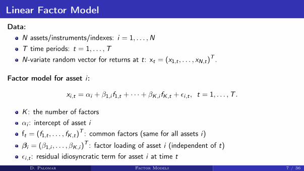
Linear Factor Model
Data:N assets/instruments/indexes: i = 1, . . . ,NT time periods: t = 1, . . . ,TN-variate random vector for returns at t: xt = (x1,t , . . . , xN,t)
T .
Factor model for asset i :
xi ,t = αi + β1,i f1,t + · · ·+ βK ,i fK ,t + εi ,t , t = 1, . . . ,T .
K : the number of factorsαi : intercept of asset ift = (f1,t , . . . , fK ,t)
T : common factors (same for all assets i)
βi = (β1,i , . . . , βK ,i )T : factor loading of asset i (independent of t)
εi ,t : residual idiosyncratic term for asset i at time t
D. Palomar Factor Models 7 / 36
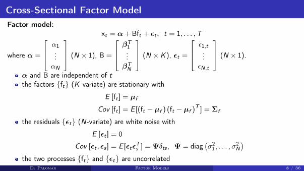
Cross-Sectional Factor ModelFactor model:
xt = α + Bft + εt , t = 1, . . . ,T
where α =
α1...αN
(N × 1), B =
βT1...
βTN
(N × K ), εt =
ε1,t...
εN,t
(N × 1).
α and B are independent of tthe factors {ft} (K -variate) are stationary with
E [ft ] = µf
Cov [ft ] = E [(ft − µf ) (ft − µf )T ] = Σf
the residuals {εt} (N-variate) are white noise with
E [εt ] = 0
Cov [εt , εs ] = E [εtεTs ] = Ψδts , Ψ = diag
(σ2
1, . . . , σ2N
)the two processes {ft} and {εt} are uncorrelated
D. Palomar Factor Models 8 / 36

Linear Factor Model
Summary of parameters:α: (N × 1) intercept for N assetsB: (N × K ) factor loading matrixµf : (K × 1) mean vector of K common factorsΣf : (K × K ) covariance matrix of K common factorsΨ = diag
(σ2
1, . . . , σ2N
): N asset-specific variances
Properties of linear factor model:the stochastic process {xt} is a stationary multivariate time series withconditional moments
E [xt | ft ] = α + BftCov [xt | ft ] = Ψ
unconditional momentsE [xt ] = α + Bµf
Cov [xt ] = BΣf BT + Ψ.
D. Palomar Factor Models 9 / 36

Multivariate Regression
Factor model (using compact matrix notation):
XT = α1T + BFT + ET
where X =
xT1...xTT
(T × N), F =
fT1...fTT
(T × K ), E =
εT1...εTT
(T × N).
D. Palomar Factor Models 10 / 36

Portfolio Analysis
Let w = (w1, . . . ,wN)T be a vector of portfolio weights (wi is the fraction of wealth in asset i).The portfolio return is
rp,t = wT rt =N∑i=1
wi ri ,t , t = 1, . . . ,T .
Portfolio factor model:
rt = α + Bft + εt ⇒rp,t = wTα + wTBft + wTεt = αp + βT
p ft + εp,t
whereαp = wTα
βTp = wTB
εp,t = wTεt
andvar(rp,t) = wT
(BΣf BT + Ψ
)w.
D. Palomar Factor Models 11 / 36

Outline
1 Introduction
2 Linear Factor Models
3 Macroeconomic Factor Models
4 Fundamental Factor Models
5 Statistical Factor Models
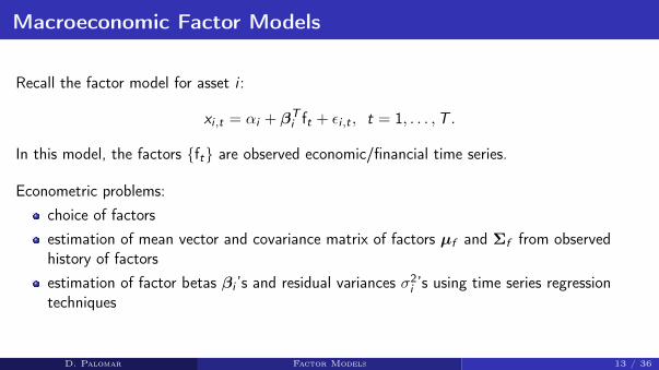
Macroeconomic Factor Models
Recall the factor model for asset i :
xi ,t = αi + βTi ft + εi ,t , t = 1, . . . ,T .
In this model, the factors {ft} are observed economic/financial time series.
Econometric problems:choice of factorsestimation of mean vector and covariance matrix of factors µf and Σf from observedhistory of factorsestimation of factor betas βi ’s and residual variances σ2
i ’s using time series regressiontechniques
D. Palomar Factor Models 13 / 36

Macroeconomic Factor Models
Single factor model of Sharpe (1964) (aka CAPM):
xi ,t = αi + βiRM,t + εi ,t , t = 1, . . . ,T
whereRM,t is the return of the market (in excess of the risk-free asset rate): market risk factor(typically a value weighted index like the S&P 500)xi ,t is the return of asset i (in excess of the risk-free rate)K = 1 and the single factor is f1,t = RM,t
the unconditional cross-sectional covariance matrix of the assets is
Cov [xt ] = Σ = σ2MββT + Ψ
whereσ2M = var (RM,t)
β = (β1, . . . , βN)T
Ψ = diag(σ2
1 , . . . , σ2N
).
D. Palomar Factor Models 14 / 36

Macroeconomic Factor Models
Estimation of single factor model:
xi = 1T αi + βi rM + εi , i = 1, . . . ,N
where rM = (RM,1, . . . ,RM,T ) with estimates:
βi = cov (xi ,t ,RM,t) /var (RM,t)
αi = xi − βi rMσ2i = 1
T−2 εTi εi , Ψ = diag
(σ2
1, . . . , σ2N
)The estimated single factor model covariance matrix is
Σ = σ2M ββT + Ψ.
D. Palomar Factor Models 15 / 36

Macroeconomic Factor Models: Market Neutrality
Recall the single factor model:
xt = α + βRM,t + εt , t = 1, . . . ,T
When designing a portfolio w, it is common to have a market-neutral constraint:
βTw = 0.
This is to avoid exposure to the market risk. The resulting risk is given by
wTΨw.
D. Palomar Factor Models 16 / 36

Capital Asset Pricing Model: AAPL vs SP500
AAPL regressed against the SP500 index (using risk-free rate rf = 2%/252):
−0.08 −0.06 −0.04 −0.02 0 0.02 0.04 0.06−0.15
−0.1
−0.05
0
0.05
0.1
Market log−return
AA
PL
lo
g−
retu
rn
Scatter
CAMP model
D. Palomar Factor Models 17 / 36

Macroeconomic Factor Models
General multifactor model:
xi ,t = αi + βTi ft + εi ,t , t = 1, . . . ,T .
where the factors {ft} represent macro-economic variables such as2
market riskprice indices (CPI, PPI, commodities) / inflationindustrial production (GDP)money growthinterest rateshousing startsunemployment
In practice, there are many factors and in most cases they are very expensive to obtain.Typically, investment funds have to pay substantial subscription fees to have access to them(not available to small investors).
2Chen, Ross, Roll (1986). “Economic Forces and the Stock Market”D. Palomar Factor Models 18 / 36

Macroeconomic Factor Models
Estimation of multifactor model (K > 1):
xi = 1Tαi + Fβi + εi , i = 1, . . . ,N
= Fγi + εi
where F =[1T F
]and γi =
[αi
βi
].
Estimates:γi = (FT F)−1FT xi , B =
[β1 · · · βN
]Tεi = xi − Fγi
σ2i = 1
T−K−1 εTi εi , Ψ = diag
(σ2
1, . . . , σ2N
)Σf = 1
T−1∑T
t=1(ft − f
) (ft − f
)T , f = 1T
∑Tt=1 ft
The estimated multifactor model covariance matrix is
Σ = BΣf BT + Ψ.D. Palomar Factor Models 19 / 36

Outline
1 Introduction
2 Linear Factor Models
3 Macroeconomic Factor Models
4 Fundamental Factor Models
5 Statistical Factor Models

Fundamental Factor Models
Fundamental factor models use observable asset specific characteristics (fundamentals) likeindustry classification, market capitalization, style classification (value, growth), etc., todetermine the common risk factors {ft}.
factor loading betas are constructed from observable asset characteristics (i.e., B is known)factor realizations {ft} are then estimated/constructed for each t given Bnote that in macroeconomic factor models the process is the opposite, i.e., the factors {ft}are given and B is estimatedin practice, fundamental factor models are estimated in two ways: BARRA approach andFama-French approach.
D. Palomar Factor Models 21 / 36

Fama-French Approach
This approach was introduced by Eugene Fama and Kenneth French (1992):For a given observed asset specific characteristics, e.g. size, determine factor realizationsfor each t with the following two steps:
1 sort the cross-section of assets based on that attribute2 form a hedge portfolio by longing in the top quintile and shorting in the bottom quintile of
the sorted assets
Define the common factor realizations with the return of K of such hedge portfolioscorresponding to the K fundamental asset attributes.Then estimate the factor loadings using time series regressions (like in macroeconomicfactor models).
D. Palomar Factor Models 22 / 36
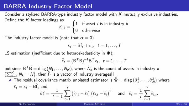
BARRA Industry Factor ModelConsider a stylized BARRA-type industry factor model with K mutually exclusive industries.Define the K factor loadings as
βi ,k =
{1 if asset i is in industry k
0 otherwise
The industry factor model is (note that α = 0)
xt = Bft + εt , t = 1, . . . ,T
LS estimation (inefficient due to heteroskedasticity in Ψ):
ft = (BTB)−1BT xt , t = 1, . . . ,T
but since BTB = diag (N1, . . . ,NK ), where Nk is the count of assets in industry k(∑K
k=1 Nk = N), then ft is a vector of industry averages!!The residual covariance matrix unbiased estimator is Ψ = diag
(σ2
1, . . . , σ2N
)where
εt = xt − Bft andσ2i =
1T − 1
T∑t=1
(εi ,t − ¯εi
) (εi ,t − ¯εi
)T and ¯εi =1T
T∑t=1
εi ,t .
D. Palomar Factor Models 23 / 36

Outline
1 Introduction
2 Linear Factor Models
3 Macroeconomic Factor Models
4 Fundamental Factor Models
5 Statistical Factor Models

Statistical Factor Models: Factor Analysis
In statistical factor models, both the common-factors {ft} and the factor loadings B areunknown. The primary methods for estimation of factor structure are
Factor Analysis (via maximum likelihood EM algorithm)Principal Component Analysis (PCA)
Both methods model the covariance matrix Σ by focusing on the sample covariance matrixΣSCM computed as follows:
XT =[x1 · · · xT
](N × T )
XT = XT
(I− 1
T1T1TT
)(demeaned by row)
ΣSCM =1
T − 1XT X.
D. Palomar Factor Models 25 / 36

Factor Analysis Model
Linear factor model as cross-sectional regression:
xt = α + Bft + εt , t = 1, . . . ,T
with E [ft ] = µf and Cov [ft ] = Σf .
Invariance to linear transformations of ft :The solution we seek for B and {ft} is not unique (this problem was not there when only Bor {ft} had to be estimated).For any K × K invertible matrix H we can define ft = Hft and B = BH−1.We can write the factor model as
xt = α + Bft + εt = α + Bft + εt
withE [ft ] = E [Hft ] = Hµf
Cov [ft ] = Cov [Hft ] = HΣfHT .
D. Palomar Factor Models 26 / 36

Factor Analysis Model
Standard formulation of factor analysis:Orthogonal factors: Σf = IKThis is achieved by choosing H = Λ−1/2ΓT , where Σf = ΓΛΓT is the spectral/eigendecomposition with orthogonal K × K matrix Γ and diagonal matrixΛ = diag (λ1, . . . , λK ) with λ1 ≥ λ2 ≥ · · · ≥ λK .Zero-mean factors: µf = 0This is achieved by adjusting α to incorporate the mean contribution from the factors:α = α + Bµf .
Under these assumptions, the unconditional covariance matrix of the observations is
Σ = BBT + Ψ.
D. Palomar Factor Models 27 / 36

Factor Analysis: MLE
Maximum likelihood estimation:Consider the model
xt = α + Bft + εt , t = 1, . . . ,T
whereα and B are vector/matrix constantsall random variables are Gaussian/Normal:
ft i.i.d. N (0, I)εt i.i.d. N (0,Ψ) with Ψ = diag
(σ2
1 , . . . , σ2N
)xt i.i.d. N
(α,Σ = BBT + Ψ
)Probability density function (pdf):
p (x1, . . . , xT | α,Σ) =T∏t=1
p (xt | α,Σ)
=T∏t=1
(2π)−N2 |Σ|−
12 exp
(−12
(xt −α)T Σ−1 (xt −α)
)D. Palomar Factor Models 28 / 36

Factor Analysis: MLE
Likelihood of the factor model:The log-likelihood of the parameters (α,Σ) given the T i.i.d. observations is
L (α,Σ) = log p (x1, . . . , xT | α,Σ)
= −TN
2log (2π)− T
2log |Σ| − 1
2
T∑t=1
(xt −α)T Σ−1 (xt −α)
Maximum likelihood estimation (MLE):
minimizeα,Σ,B,Ψ
T2 log |Σ|+ 1
2∑T
t=1 (xt −α)T Σ−1 (xt −α)
subject to Σ = BBT + Ψ
Note that without the constraint, the solution would be
α =1T
T∑t=1
xt and Σ =1T
T∑t=1
(xt − α) (xt − α)T .
D. Palomar Factor Models 29 / 36

Factor Analysis: MLE
MLE solution:
minimizeα,Σ,B,Ψ
T2 log |Σ|+ 1
2∑T
t=1 (xt −α)T Σ−1 (xt −α)
subject to Σ = BBT + Ψ
Employ the Expectation-Maximization (EM) algorithm to compute α, B, and Ψ.Estimate factor realization {ft} using, for example, the GLS estimator:
ft = (BT Ψ−1B)−1BT Ψ−1xt , t = 1, . . . ,T .
The number of factors K can be estimated with a variety of methods such as the likelihoodratio (LR) test, Akaike information criterion (AIC), etc. For example:
LR(K ) = −(T − 1− 16
(2N + 5)− 23K )(
log |ΣSCM| − log |BBT + Ψ|)
which is asymptotically chi-square with 12((N − K )2 − N − K ) degrees of freedom.
D. Palomar Factor Models 30 / 36

Principal Component Analysis
PCA: is a dimension reduction technique used to explain the majority of the information in thecovariance matrix.
N-variate random variable x with E [x] = α and Cov [x] = Σ.Spectral/eigen decomposition Σ = ΓΛΓT where
Λ = diag (λ1, . . . , λK ) with λ1 ≥ λ2 ≥ · · · ≥ λKΓ orthogonal K × K matrix: ΓTΓ = IN
Principal component variables: p = ΓT (x−α) with
E [p] = E[ΓT (x−α)
]= ΓT (E [x]−α) = 0
Cov [p] = Cov[ΓT (x−α)
]= ΓTCov [x]Γ = ΓTΣΓ = Λ.
p is a vector of zero-mean, uncorrelated random variables, in order of importance (i.e., thefirst components explain the largest portion of the sample covariance matrix)In terms of multifactor model, the K most important principal components are the factorrealizations.
D. Palomar Factor Models 31 / 36

Factor Models: Principal Component Analysis
Factor model from PCA:From PCA, we can write the random vector x as
x = α + Γp
where E [p] = 0 and Cov [p] = Λ = diag (Λ1,Λ2).Partition Γ =
[Γ1 Γ2
]where Γ1 corresponds to the K largest eigenvalues of Σ.
Partition p =
[p1p2
]where p1 contains the first K elements
Then we can writex = α + Γ1p1 + Γ2p2 = α + Bf + ε
whereB = Γ1, f = p1 and ε = Γ2p2.
This is like a factor model except that Cov [ε] = Γ2Λ2ΓT2 , where Λ2 is a diagonal matrix
of last N − K eigenvalues but Cov [ε] is not diagonal...D. Palomar Factor Models 32 / 36

Factor Models: Why PCA?
But why is PCA the desired solution to the statistical factor model?The idea is to obtain the factors from the returns themselves:
xt = α + Bft + εt , t = 1, . . . ,T
ft = CT xt + d
or, more compactly,
xt = α + B(CT xt + d
)+ εt , t = 1, . . . ,T
The problem formulation is
minimizeα,B,C,d
1T
∑Tt=1 ‖xt −α + B
(CT xt + d
)‖2
Solution is involved to derive and is given by: ft = ΓT1 (xt −α) or, if normalized factors
are desired, ft = Λ− 1
21 ΓT
1 (xt −α).D. Palomar Factor Models 33 / 36

Factor Models via PCA
1 Compute sample estimates
α =1T
T∑t=1
xt and Σ =1T
T∑t=1
(xt − α) (xt − α)T .
2 Compute spectral decomposition:
Σ = ΓΛΓT , Γ =[Γ1 Γ2
]3 Form the factor loadings, factor realizations, and residuals (so that xt = α + Bft + εt):
B = Γ1Λ121 , ft = Λ
− 12
1 ΓT1 (xt − α) , εt = xt − α− Bft
4 Covariance matrices:
Σf =1T
T∑t=1
ft fTt = IK , Ψ =1T
T∑t=1
εt εTt = Γ2Λ2Γ2 (not diagonal!)
Σ = Γ1Λ1Γ1 + Γ2Λ2Γ2 = BΣf BT + Ψ.D. Palomar Factor Models 34 / 36
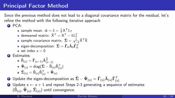
Principal Factor Method
Since the previous method does not lead to a diagonal covariance matrix for the residual, let’srefine the method with the following iterative approach
1 PCA:sample mean: α = x = 1
T XT1Tdemeaned matrix: XT = XT − x1TTsample covariance matrix: Σ = 1
T−1 XT Xeigen-decomposition: Σ = Γ0Λ0Γ
T0
set index s = 02 Estimates:
B(s) = Γ(s−1)Λ12(s−1)
Ψ(s) = diag(Σ− B(s)BT(s))
Σ(s) = B(s)BT(s) + Ψ(s)
3 Update the eigen-decomposition as Σ− Ψ(s) = Γ(s)Λ(s)ΓT(s)
4 Update s ← s + 1 and repeat Steps 2-3 generating a sequence of estimates(B(s), Ψ(s), Σ(s)) until convergence.
D. Palomar Factor Models 35 / 36

Thanks
For more information visit:
https://www.danielppalomar.com
Top Related