


Languages
Pages
Legal


University of Arkansas, FayettevilleScholarWorks@UARK
Theses and Dissertations
5-2013
Expression, Production, and Purification of NovelTherapeutic ProteinsMckinzie Shea FruchtlUniversity of Arkansas, Fayetteville
Follow this and additional works at: http://scholarworks.uark.edu/etd
Part of the Biochemical and Biomolecular Engineering Commons, Biochemistry Commons, andthe Biotechnology Commons
This Dissertation is brought to you for free and open access by ScholarWorks@UARK. It has been accepted for inclusion in Theses and Dissertations byan authorized administrator of ScholarWorks@UARK. For more information, please contact [email protected], [email protected].
Recommended CitationFruchtl, Mckinzie Shea, "Expression, Production, and Purification of Novel Therapeutic Proteins" (2013). Theses and Dissertations.701.http://scholarworks.uark.edu/etd/701

EXPRESSION, PRODUCTION, AND PURIFICATION OF NOVEL THERAPEUTIC PROTEINS
EXPRESSION, PRODUCTION, AND PURIFICATION OF NOVEL THERAPEUTIC PROTEINS
A dissertation submitted in partial fulfillment of the requirements for the degree of
Doctor of Philosophy in Chemical Engineering
By
McKinzie S. Fruchtl Hendrix College
Bachelor of Arts in Mathematics, 2008
May 2013 University of Arkansas

ABSTRACT
Interest in the production of recombinant proteins consisting of collagen binding domain
(CBD) fused to a bioactive material has increased due to the targeting/attachment capabilities of
CBD. For example, CBD fusions can be applied to the reversing of bone density loss and the
repair of the eardrum, specifically, by choosing an appropriate fusion partner (parathyroid
hormone or epidermal growth factor). The production of CBD fusions was examined using
batch and fed-batch culturing of Escherichia coli to express the fusion proteins, and affinity
chromatography to isolate the final product.
Different medium formulations, feeding strategies, and induction methods were tested in
order to develop a production strategy lacking yeast extract or other difficult-to-validate
materials. Lactose was also examined as an alternative inducer to IPTG due to its lower cost and
toxicity. This induction strategy, in conjunction with alternative feeding methods and the use of
a completely defined medium, was able to produce the desired fusion proteins in a comparable
manner to IPTG-induced systems. Also, the affinity tag on the N-terminus of the protein and the
collagen binding domain on the C-terminus of the protein both retained their activity throughout
the fermentation and purification processes.
The second portion of this dissertation examined and utilized two different types of
models to mathematically describe the biological system. The first model was able to describe
the fermentation system with respect to changes in feed, volume, biomass, and carbohydrate
concentrations. This type of modeling examined the entire physical fermentation system on a
'macro' scale. Unlike the second model, it disregarded what occurred on a cellular level.
The second model utilized metabolic flux analysis to track changes in metabolite
concentrations and biomass during the expression of the target protein. Upon solving this model,
the prediction of the intermediate fluxes proved to be accurate for glucose-fed experiments, as
the simulated carbohydrate concentrations match those that were experimentally determined.
With the inclusion of the models, the work described in this dissertation provided a link between
experimentally observed phenomena and mathematical descriptions of biological systems.

This dissertation is approved for recommendation
to the Graduate Council.
Dissertation Director:
_______________________________
Dr. Robert R. Beitle
Dissertation Committee:
_______________________________
Dr. Edgar Clausen
_______________________________
Dr. Ralph Henry
_______________________________
Dr. Christa Hestekin
_______________________________
Dr. Shannon Servoss
DISSERTATION DUPLICATON RELEASE
I hereby authorize the University of Arkansas Libraries to duplicate this dissertation when
needed for research and/or scholarship.
Agreed _______________________________
McKinzie S. Fruchtl
Refused _______________________________
McKinzie S. Fruchtl

ACKNOWLEDGEMENTS
First and foremost, I would like to thank my advisor. Dr. Beitle is one of the most
positive people I know. There were some experiments that I thought were complete failures, but
he always managed to pull out the positive aspects. I don't know where I would be today if it
weren't for him (and a happenstance meeting between his wife and my mother at a grocery store
- so thanks to them too!). In all honesty, I couldn't have asked for a better mentor and friend in
the research field and I can't fully express how grateful I am that I got the opportunity to work
with him. I am one of the lucky ones!
I would also like to thank my committee members for their contributions to my work.
Through the various update meetings, they were able to help troubleshoot portions of my work
when I needed help and keep me on track.
Lastly, I thank my family and friends. It was a long five years and a rough road at times.
They remained supportive and managed to see the light in every situation. I'm sure they got tired
me ranting about lab issues and talking about mathematical modeling, but they smiled and
nodded when I needed it most. They encouraged me to keep going and hang in there. I share my
success with them.
TABLE OF CONTENTS
List of Figures
List of Tables
1. Overview 1
2. Background 1
2.1 Bioprocessing and Fermentation 1
2.2 Media 3
2.3 Fed-batch fermentation 4
2.3.1 Effect of acetate on the cellular system 8
2.3.2 Feed type 13
2.3.3 Strategies for the control of feeding 14
2.4 Expression and production 18
2.4.1 Lac operon 19
2.4.2 Simple induction strategies 22 2.4.3 Auto-induction 26
2.5 Dynamic modeling and metabolic flux analysis 29
2.6 Purification 38
2.7 Medically relevant CBD-fusions as test cases for dissertation 40
2.7.1 PTH-CBD 42
2.7.2 EGF-CBD 43
3. Specific Aims 44
4. Materials and Methods 47
4.1 Strains and plasmids 47
4.2 Media 48
4.3 Shake flask cultivations 48
4.4 Batch cultivations 51
4.5 Fed-batch cultivations 52
4.6 Lysate preparation 59
4.7 Analytical assays 60
4.7.1 Cell growth and fermentation conditions 60
4.7.2 Carbohydrate determination 60
4.7.3 Protein analysis 61
4.8 Fast protein liquid chromatography (FPLC) 63
4.9 Activity analysis 63
4.10 Dynamic modeling 64
4.11 Metabolic flux analysis 67
5. Results and Discussion 80
5.1 Shake flask cultivations 80
5.2 Batch cultivations 91
5.3 Fed-batch cultivations 92
5.3.1 Cultures fed with glucose as major carbon source 93
5.3.1.1 Lactose induction after inoculation 93
5.3.1.2 Auto-induction with lactose 109 5.3.1.3 IPTG induction 119
5.3.1.3 IPTG induction 119
5.3.2 Cultures fed with glycerol as major carbon source 128
5.3.2.1 Lactose induction after inoculation 128
5.3.2.2 Auto-induction with lactose 134
5.4 Cost analysis 146
5.5 Summary of fed-batch fermentation experiments 152
5.6 Fine analysis of product 158
5.7 Purification, activity analysis, and cleavage 160
6. Simulations 164 164
6.1 Dynamic modeling 164
6.2 Metabolic flux analysis 179
7. Conclusions and recommendations 197
8. References 200
9. Appendix 209

List of Figures
Figure 2-1: Schematic of fed-batch fermentation set-up. .............................................................. 6
Figure 2-2: Example of pH profile during fed-batch fermentation .............................................. 15
Figure 2-3: Dissolved oxygen profile during fed-batch fermentation. ........................................ 16
Figure 2-4: Cartoon of lac operon ............................................................................................... 20
Figure 2-5: Chromatogram for GST-tagged protein .................................................................... 40
Figure 2-6: Translocation of PTH-CBD after subcutaneous injection in mice. .......................... 43
Figure 3-1: Flow chart of how experiments proceeded. .............................................................. 45
Figure 4-1: Plasmid map of pCHC305 ........................................................................................ 47
Figure 4-2: Linear correlations between optical density and Bugeye output .............................. 53
Figure 4-3: Image of program utilizing exponential feeding algorithm ...................................... 54
Figure 4-4: Image of program utilizing regulatory feeding algorithm ........................................ 57
Figure 4-5: Analysis of SDS-PAGE gel using densitometry ....................................................... 62
Figure 4-6: Metabolic pathways with lactose consumption and glucose feed ............................. 68
Figure 4-7: Metabolic pathways with lactose consumption and glycerol feed ............................ 69
Figure 4-8: Metabolic pathways with glycerol as only carbohydrate present in media .............. 71
Figure 5-1: Comparison of growth on LB or LB + glucose. ....................................................... 81
Figure 5-2: Comparison of protein expression on LB or LB + glucose ...................................... 81
Figure 5-3: GST-PTH-CBD expression from cells grown on LB or M9 .................................... 82
Figure 5-4: Western blot from lactose or IPTG induction with M9 + glucose media ................. 84
Figure 5-5: Growth of LB vs. M9 + glucose supplemented with amino acids ............................ 85
Figure 5-6: Growth curve of induced cultures on M9 supplemented with amino acids .............. 86
Figure 5-7: Protein from M9 + glucose with amino acids induced for 4 hrs. .............................. 87
Figure 5-8: Protein from M9 + glucose with amino acids induced for 22 hrs ............................. 88
Figure 5-9: HPLC analysis of glucose and lactose for auto-induction in shake flasks ................ 90
Figure 5-10: Batch growth data for different inducers ................................................................ 91
Figure 5-11: Growth for saw-tooth feeding method .................................................................... 93
Figure 5-12: Western blot of lysates from saw-tooth feeding method ........................................ 94
Figure 5-13: Protein and feed profile versus time for saw-tooth method. ................................... 96
Figure 5-14: Carbons versus time for saw-tooth feeding strategy ............................................... 97
Figure 5-15: Fed-batch growth curve for un-induced cultures (μ = 0.2hr-1
) .............................. 98
Figure 5-16: Growth for fermentations induced with lactose 12 hours after inoculation ............ 99
Figure 5-17: Protein for fermentations induced 12 hours after inoculation ............................... 101
Figure 5-18: Carbons for cultures induced with lactose 12 hours after inoculation .................. 103
Figure 5-19: Growth for cultivation induced when feed started ................................................ 104
Figure 5-20: Protein for cultivations induced with lactose when feed started ........................... 105
Figure 5-21: Carbons for cultivations induced with lactose when feed started ......................... 107
Figure 5-22: Growth of auto-induced cultures........................................................................... 109
Figure 5-23: Protein with respect to time for auto-induced cultures ......................................... 110
Figure 5-24: Carbons for auto-induced fed-batch fermentations ............................................... 112
Figure 5-25: Growth from auto-induced fermentation with lactose pulse. ................................ 113
Figure 5-26: Protein from auto-induction with additional pulsing of lactose ............................ 115
Figure 5-27: Carbons for auto-induction with lactose pulse ...................................................... 117
Figure 5-28: Western blot of lysate from AI cultures with pulse .............................................. 118
Figure 5-29: Growth curve for 5 mM IPTG-induced culture. ................................................... 119
Figure 5-30: Protein for 5 mM IPTG-induced cultivations ....................................................... 121
Figure 5-31: Carbons for 5 mM IPTG-induced cultures. .......................................................... 123
Figure 5-32: Growth curve for 10 mM IPTG-induced cultures ................................................. 120
Figure 5-33: Protein for 10 mM IPTG-induced cultures ........................................................... 125
Figure 5-34: Carbons for cultures induced with 10 mM IPTG. ................................................. 127
Figure 5-35: Growth for glycerol-fed cultivations with 15 g lactose added at feed start. ......... 129
Figure 5-36: Protein for glycerol-fed cultures with 15 g lactose at feed start ........................... 130
Figure 5-37: Carbons for glycerol-fed cultures with 15 g of lactose ......................................... 133
Figure 5-38: Growth for auto-induced cultures with glycerol feed ........................................... 134
Figure 5-39: Proteins for auto-induced cultures with glycerol feed .......................................... 136
Figure 5-40: Carbons for auto-induced with glycerol feed ........................................................ 138
Figure 5-41: Growth for glycerol-fed auto-induced cultures with lactose pulse. ...................... 141
Figure 5-42: Protein for glycerol-fed auto-induced cultures with lactose pulse ........................ 143
Figure 5-43: Carbons for glycerol-fed auto-induced cultures with lactose pulse ...................... 145
Figure 5-44: Average cell weights for different fed-batch induction techniques ...................... 154
Figure 5-45: SDS-PAGE gel with β-lactamase band ................................................................. 159
Figure 5-46: SDS-PAGE gel with purified fractions ................................................................. 161
Figure 5-47: Western blot with purified fractions ..................................................................... 161
Figure 5-48: Activity analysis for GST-PTH-CBD ................................................................... 162
Figure 5-49: SDS-PAGE gel indicating cleavage of tag ........................................................... 163
Figure 6-1: Dynamic model simulation with experimental data ............................................... 168
Figure 6-2: Dynamic model simulation with alternative lactose equation ................................ 170
Figure 6-3: Dynamic model simulation without acetate equation ............................................. 173
Figure 6-4: Simulated profiles using glucose with alternative lactose equation ....................... 175
Figure 6-5: Simulated profiles using alternative glucose with original lactose equation .......... 176
Figure 6-6: Simulated profiles using alternative carbohydrate equations ................................. 177
Figure 6-7: Simulated fluxes from 12 hr lactose-induced cultures (glucose-fed) ..................... 181
Figure 6-8: Simulated fluxes from auto-induced with pulse cultures (glucose-fed) ................. 182

List of Tables
Table 2-1: Summary of how changes on the genetic level affect acetic acid production ............ 10
Table 2-2: Variables, units, and description of variables in dynamic model ............................... 33
Table 4-1: Amino acid composition of GST-PTH-CBD ............................................................. 50
Table 4-2: Summary of fed-batch fermentation experiments ...................................................... 59
Table 4-3: Synthesis of monomers from metabolic precursors ................................................... 75
Table 4-4: Metabolic costs for production of GST-PTH-CBD ................................................... 76
Table 5-1: Summary of experiments performed with lactose-induction. .................................. 108
Table 5-2: Summary of experiments using glucose as a feed source ........................................ 127
Table 5-3: Comparison of lactose induction when feed started with respect ot feed type ........ 131
Table 5-4: Comparison of auto-induced experiments with respect to feed type ....................... 137
Table 5-5: Comparison of auto-induced experiments with lactose pulse .................................. 145
Table 5-6: Cost analysis of fed-batch fermentation experiments .............................................. 146
Table 5-7: Number of fermentations required to produce protein from 10 mM IPTG runs ...... 148 Table 5-8: Requirement of fermentations to make one gram of product ................................... 149
Table 5-9: Cost breakdown for production of one gram of product .......................................... 150
Table 5-10: Final dry cell weights with respect to fermentation method .................................. 152
Table 5-11: Protein production with respect to fermentation method ....................................... 153
Table 5-12: Yield of biomass from carbon with respect to fermentation method ..................... 156
Table 6-1: Amino acid consumption after 16 hours for 12 hr lactose induction ....................... 179
Table 6-2: Fluxes for each glucose-fed fermentation ................................................................ 184
Table 6-3: Fluxes between each time step for 12 hr lactose induction ...................................... 185
Table 6-4: Predicted vs. experimental concentrations for 12 hr lacotse induction .................... 186
Table 6-5: Fluxes for IPTG-induced experiments ..................................................................... 187
Table 6-6: Predicted vs. experimental concentrations for IPTG and AI w/pulse cultures ........ 188
Table 6-7: Flux data from glycerol-fed experiments ................................................................. 190
Table 6-8: Predicted vs. experimental concentrations for glycerol-fed cultures ....................... 191
Table 6-9: Required glycerol uptake rates to match experimental data ..................................... 193 Table 6-10: Fluxes used in ATP yield calculations ................................................................... 194
Table 6-11: Contribution of energetics to ATP yield calculations ............................................ 194 Table 6-12: Ratios of ATP yields and biomass yields ............................................................... 196

1
1. Overview
A novel therapeutic fusion protein has been shown to increase bone density and decrease
hair loss. The fusion protein consists of parathyroid hormone (PTH) bound to collagen-binding
domain (CBD). In this case, collagen-binding domain serves as a vehicle for attachment to
tissues, while also increasing the half-life of the parathyroid hormone. In preparation for scale-
up procedures, production and expression of this protein were investigated. Induction studies
were carried out to find the conditions allowing for the greatest amount of recombinant protein
expression.
To ease the purification process, a glutathione-S-transferase (GST) tail has been placed
on the N-terminus of the PTH-CBD protein complex. Affinity chromatography was used to
separate the target protein from the pool of bacterial proteins. After production and purification
of GST-PTH-CBD, dynamic modeling was utilized to model the cultivation process and
metabolic flux analysis was used to model the changes in metabolite concentrations during the
expression of the target protein. Additionally, the model contains information about the effect of
the inducer on the fermentation system as a whole.
2. Background
2.1 Bioprocessing and fermentation
Bioprocessing refers to the production of a commercially useful biomaterial from a
biological process. In the context of this dissertation, it refers to the production of proteins via
the fermentation process of a genetically engineered microbial strain. The proteins of particular
interest have therapeutic applications and can be used in the biopharmaceutical industry.
Because the success of any biopharmaceutical product depends on the ability to engineer large-
2
scale manufacturing protocols, there is a desire to increase production of these therapeutic
proteins using bioprocessing methods (Tripathi et al., 2009).
For this work, fermentation refers to the breakdown of glucose under aerobic conditions
by Escherichia coli to produce a variety of substrates. Of particular interest is the production of
proteins. The goal of recombinant fermentation processes is to engineer cost effective
production of target proteins by increasing yield in the smallest amount of materials and/or time
(Tripathi et al., 2009). This is achieved by using a stable and highly productive fermentation
process followed by cost effective recovery and purification of the product (Tripathi et al., 2009).
E.coli is perhaps the most widely used bacteria for the production of recombinant
proteins (Babaeipour et al., 2008; Choi et al., 2006; Lee, 1996; Shiloach and Fass, 2005).
Because of its simple structure, the vast information available on this species, and its inexpensive
production methods, it is the microorganism of choice for the production of recombinant proteins
(Choi et al., 2006; Kayser et al., 2005; Lee, 1996; Tripathi et al., 2009). E. coli is primarily used
for cloning, genetic modification, and small-scale production specifically for research purposes
(Ferrer-Miralles et al., 2009). However, the production of recombinant proteins in E. coli is most
important because of its application in the pharmaceutical industry (Meadows et al., 2010).
Demand for these products has increased because of their functionality in the therapeutic and
diagnostic fields (Tripathi et al., 2009). Recombinant protein production from genetically
modified organisms is also the largest sector of pharmaceutical biotechnology (Behme, 2009).
3
2.2 Media
The type of medium plays a very important role in the fermentation process, as some
common medium components can inhibit growth if their concentration becomes too high. As
reported by Lee et al., glucose concentrations at about 50 g/L can inhibit E. coli growth.
Similarly, ammonia levels above 3 g/L, iron levels exceeding 1.15 g/L, zinc levels above 0.038
g/L, magnesium levels above 8.7 g/L and phosphorous levels greater than 10 g/L can all inhibit
cellular growth (Lee, 1996; Shiloach and Fass, 2005). These numbers are important to consider
when designing growth media because the optimal medium would use concentrations of
nutrients that remain above the growth-limiting level (concentrations too low) and below the
toxic level (concentrations too high), while not leading to wasteful expenditure (Faulkner et al.,
2006).
There are three different types of media: defined, semi-defined, and complex. Defined
media are used most often to achieve high cell densities (Lee, 1996). This is because each
component is clearly defined and the concentration of these components can be tightly controlled
throughout the culture process. Defined media are comprised mostly of different types of salts
and some type of trace element solution (provides iron, zinc, copper, and other cofactors that
cells need). Complex media, on the other hand, contain extremely nutrient rich components and
the exact composition may be unknown. Examples of complex media are Luria-Burtani (LB)
broth, peptone-based media, and media that may contain yeast extract and tryptone. The exact
chemical make-up of these can vary from lot-to-lot, making scale-up and reproducibility more
difficult than that of a fermentation protocol utilizing defined medium.
4
When growth or protein expression does not occur on a clearly defined medium, a
combination of the two can be used. Semi-defined media may be used to increase product
formation or decrease acetate production (Eiteman and Altman, 2006; Lee, 1996). For high cell
density cultivations, it is important to use a medium that allows for higher growth rates while
avoiding by-production formation (such as acetate). Though acetate formation is largely
dependent on the strain of bacteria, it has been reported that acetate forms when the specific
growth rate (dilution rate) exceeds 0.2 hr-1
and 0.35 hr-1
for growth on complex media and
defined media, respectively (Han et al., 1992; Lee, 1996; Tripathi et al., 2009). These numbers
are important to considering when designing a fermentation scheme. For batch cultivations,
higher growth rates will decrease the ability for the media to sustain growth for longer periods of
time. Acetate will also accumulate faster. Through the use of fed-batch fermentation, as
discussed below, the culture can be maintained for a greater amount of time at a faster growth
rate (Longobardi, 1994).
2.3 Fed-batch fermentation
In order to achieve high cell density cultures of E. coli, which result in high yields and
productivity of recombinant proteins, fed-batch fermentation must be utilized. According to
Tripathi et al., high cell density fermentation "is a major bio-process engineering consideration
for enhancing the overall yield of recombinant proteins in E. coli" (Tripathi et al., 2009). Fed-
batch processes are utilized to achieve higher cell concentrations while minimizing problems that
can arise from high cell density cultivations, such as substrate or product inhibition, nutrient
inhibition, or dissolved oxygen limitations in aerobic conditions (Ting et al., 2008). Fed-batch
fermentation also provides an increase in productivity, which drives a decrease in manufacturing

5
cost (Longobardi, 1994). Without fed-batch fermentation, cell densities of E. coli may approach
15 g/l dry cell weight (DCW) on defined media, provided the nutrient concentrations remain
below their inhibitory concentrations (Shiloach and Fass, 2005). In contrast, dry cell weights can
approach over ten times this amount through the utilization of a feeding method during
cultivation.
Fed-batch processing also permits control of the feed rate of glucose into the cultivation,
which results in greater control on the growth rate of the culture (Ting et al., 2008). This helps
control biomass accumulation at growth rates which do not cause the formation of acetic acid, a
byproduct capable of inhibiting cell growth at concentrations as low as 2 g/l, depending on the
strain (Shiloach and Fass, 2005). When acetate exceeds 5 g/l there is a definite negative impact
on growth and most groups report on witnessing inhibition of growth when acetate reaches
concentrations between 5 and 10 g/l (Tripathi et al., 2009; Yee and Blanch, 1993).
Different fed-batch feeding strategies also allow for different growth rates. The objective
is to optimize the feeding strategy so that there is a balance between high growth rates and
limiting factors that can arise as a result of these high growth rates. The control of the growth
rate is important in fed-batch fermentation because it effects byproduct formation, cell
productivity, and plasmid stability (Faulkner et al., 2006). Hence, the optimal feeding strategy
would feed nutrient in at the same rate that the organism consumes the substrate (Kleman et al.,
1991). Other considerations include the dosing of ammonia. It supplies nitrogen to the system
while also maintaining the desired pH. In short, fed-batch processing allows one to monitor and
adjust concentrations so that they remain supportive instead of inhibitory. A simple fed-batch
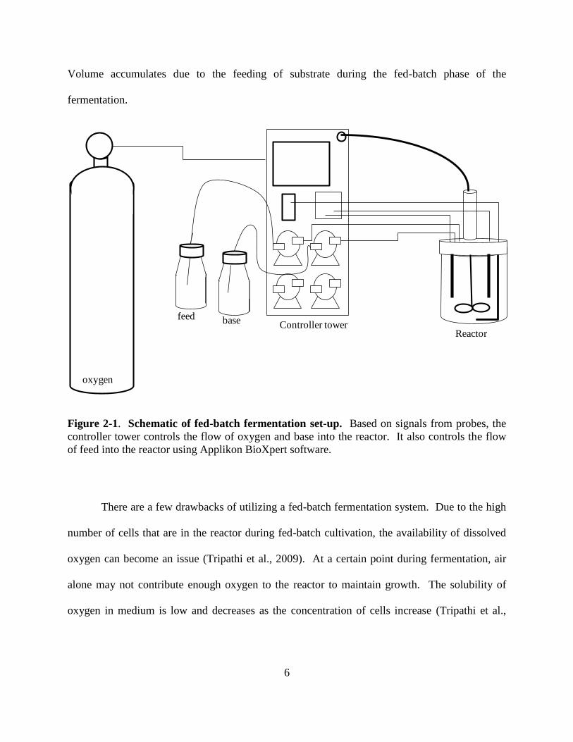
fermentation schematic is shown in Figure 2-1. The system utilizes a simple stirred-tank reactor.
6
Volume accumulates due to the feeding of substrate during the fed-batch phase of the
fermentation.
Figure 2-1. Schematic of fed-batch fermentation set-up. Based on signals from probes, the
controller tower controls the flow of oxygen and base into the reactor. It also controls the flow
of feed into the reactor using Applikon BioXpert software.
There are a few drawbacks of utilizing a fed-batch fermentation system. Due to the high
number of cells that are in the reactor during fed-batch cultivation, the availability of dissolved
oxygen can become an issue (Tripathi et al., 2009). At a certain point during fermentation, air
alone may not contribute enough oxygen to the reactor to maintain growth. The solubility of
oxygen in medium is low and decreases as the concentration of cells increase (Tripathi et al.,
oxygen
basefeed
ReactorController tower
7
2009). Pure oxygen would need to be supplied in this case, or the agitation speed would need to
be increased.
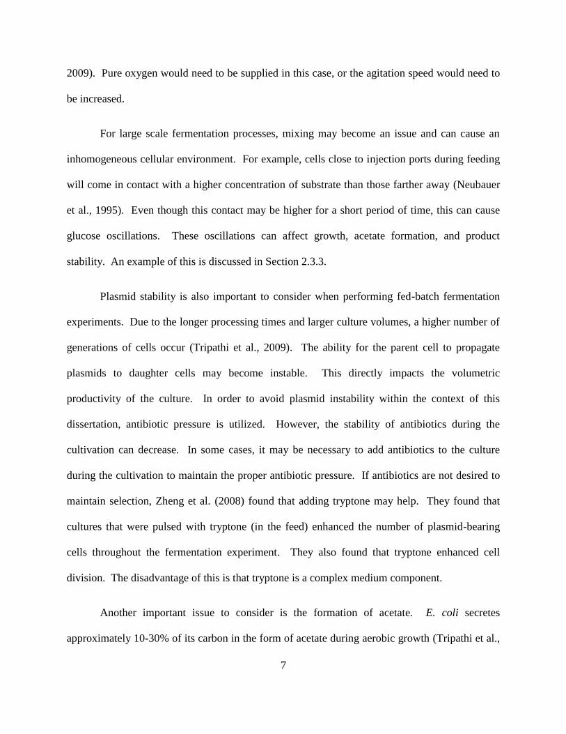
For large scale fermentation processes, mixing may become an issue and can cause an
inhomogeneous cellular environment. For example, cells close to injection ports during feeding
will come in contact with a higher concentration of substrate than those farther away (Neubauer
et al., 1995). Even though this contact may be higher for a short period of time, this can cause
glucose oscillations. These oscillations can affect growth, acetate formation, and product
stability. An example of this is discussed in Section 2.3.3.
Plasmid stability is also important to consider when performing fed-batch fermentation
experiments. Due to the longer processing times and larger culture volumes, a higher number of
generations of cells occur (Tripathi et al., 2009). The ability for the parent cell to propagate
plasmids to daughter cells may become instable. This directly impacts the volumetric
productivity of the culture. In order to avoid plasmid instability within the context of this
dissertation, antibiotic pressure is utilized. However, the stability of antibiotics during the
cultivation can decrease. In some cases, it may be necessary to add antibiotics to the culture
during the cultivation to maintain the proper antibiotic pressure. If antibiotics are not desired to
maintain selection, Zheng et al. (2008) found that adding tryptone may help. They found that
cultures that were pulsed with tryptone (in the feed) enhanced the number of plasmid-bearing
cells throughout the fermentation experiment. They also found that tryptone enhanced cell
division. The disadvantage of this is that tryptone is a complex medium component.
Another important issue to consider is the formation of acetate. E. coli secretes
approximately 10-30% of its carbon in the form of acetate during aerobic growth (Tripathi et al.,
8
2009). If cells cannot convert the glucose entering the reactor to a desirable product fast enough,
the extra carbon often gets secreted as acetate. Problems that arise from this are described in
detail in the next section.
2.3.1 Effect of acetate on the cellular system
Acetate, a harmful byproduct of fermentation, is produced via two pathways under
aerobic conditions. When the conversion of the primary carbon source (glucose) to biomass and
carbon dioxide is less than its uptake rate acetate excretion occurs (Kleman and Strohl, 1994).
Acetate excretion from this build-up of glucose in the media is referred to as overflow
metabolism (Akesson et al., 2001). Acetate excretion also occurs when there is a lack of
dissolved oxygen in the medium (De Mey et al., 2007). Under this anaerobic condition, the
formation of acetic acid is referred to as mixed-acid fermentation (Akesson et al., 2001). As
previously stated, acetate can inhibit cell growth at concentrations as low as 2 g/l. High acetate
levels can also lower biomass yield, negatively affect the maximum attainable cell density, and
decrease the production of recombinant protein (Lee, 1996). Additionally, the build-up of
acetate can have detrimental effects on the stability of intracellular proteins and cause the growth
medium to acidify (De Mey et al., 2007). If the pH drops too low, cell lysis can occur.
As previously discussed, the rate of production of acetate is strain dependent and acetate
production begins at a lower growth rate (0.2 hr-1
) when the medium is complex (nutrient-rich)
as opposed to that when the medium is defined (0.35 hr-1
). To eliminate or reduce the build-up
of acetic acid, there are two levels at which researchers have developed strategies: the genetic
level and the bioprocess level (De Mey et al., 2007). At the genetic level, multiple research
groups have looked at knocking out the genes that can lead to acetic acid excretion or
9
overexpressing genes that can cause a decrease in acetic acid formation. The strategies are based
on the metabolism of E. coli and begin with changing the glucose uptake mechanism and the
TCA cycle. The pyruvate branch point is also an important area to point out because the
pyruvate concentration has an immediate influence on the excretion of acetate, according to De
Mey et. al (2007). This branch point is also affected by the aforementioned pathway between
glycolysis and the TCA cycle. From pyruvate, the genes directly affecting acetate production are
examined for knockout or overexpression. Table 2.1 gives examples of genes that have been
knocked out, overexpressed, inhibited, or stimulated and the effects that these actions had on
acetic acid formation.
Another interesting approach using genetic modifications to reduce acetic acid
concentrations was brought to light by Aristidou et al. (1995). They cloned the gene for
acetolactate synthase (from Bacillus subtilis) in E. coli. This enzyme is capable of catalyzing
pyruvate to non-acidic less harmful byproducts (compared to acetic acid). They reported a 220%
increase in volumetric protein production and a 35% higher cell density using the acetolactate
synthase modified strain.

10
Table 2-1. Summary of how changes on the genetic level affect acetic acid production. KO
refers to knockout; OE refers to overexpression; I refers to inhibition; and Stim refers to
stimulation. Table adapted from De Mey et al. (2007).
Pathway Gene Protein Action Result
Phospho-
transferase
pathway
ptsG Glucose Specific
Enzyme II
KO Glucose uptake reduced; no
acetate excretion
arcA Regulator of ptsG KO 2x increase in ptsG
OE Glucose uptake decrease; decrease
in acetate
Pyruvate
branch point
pykF Pyruvate kinase KO Glycolysis down regulated;
decrease in acetate
pykA
pykF
Pyruvate kinase KO Major decrease in growth rate and
acetate
pdh Pyruvate
dehydrogenase
I Decrease in growth rate; no
acetate production
ppc Phosphoenolpyruvate
(PEP) carboxylase
OE Elimination of acetate production;
growth is maintained; decrease in
glucose consumption rate
KO Decrease is growth rate;
undesirable metabolite production
increases
pck PEP carboxykinase KO No acetate production from
growth on high glucose
concentrations
OE Slight raise in acetate production
ppc
pck
PEP carboxylase and
PEP carboyxkinase
OE Less growth; higher concentration
of fermentative products
pta phosphotransacetylase KO Reduction in acetate; growth rate
suffers; increase in lactate and
formate ackA Acetate kinase KO
acs Acetyl-CoA
Synthetase
KO No precise conclusion
OE Reduction in acetate; increase
assimilation of acetate when sole
carbon source
poxB Pyruvate oxidase KO Decrease in carbon to biomass;
carbon needed for energy
increased
gltA Citrate synthase OE Decrease in acetate; increase in
formate and pyruvate
aceA Isocitrate lyase Stim Decrease in acetate by 13%
icd Isocitrate
dehydrogenase
KO Increase in citrate; not rate
limiting step in Krebs cycle
11
Manipulation to reduce acetate at the bioprocess level mainly deals with media
formulation and/or cultivation techniques. Many groups have reported on adding yeast extract to
the media in order to reduce acetate accumulation during fermentation (Eiteman and Altman,
2006; Han et al., 1992; Tripathi et al., 2009). Yeast extract acts an alternative food source
(nitrogen rich), so it slows the uptake rate of glucose, which decreases acetic acid formation.
Panda et al. found that through the use of yeast extract, glucose uptake rate was lowered, but
growth was not affected. It also helped maximize the volumetric productivity of the
fermentation and produced less acetic acid (Panda et al., 2000). Reportedly, yeast extract also
helps E. coli utilize acetate acid during carbon limitation (Tripathi et al., 2009). However, the
addition of yeast extract would push the medium to a semi-defined medium, which is not
desirable for the work in this dissertation. de Maré et al. (2005) examined the use of shifting
temperatures in correspondence with oxygen changes to monitor the production of acetic acid.
Decreasing the temperature helped control the oxygen consumption rate which in turn resulted in
lower acetic acid concentrations. This may be due to slower glucose uptake and slower growth,
but the group reported a 20% increase in cell mass using this technique.
To physically remove acetate from the culture broth, some groups have looked at
utilizing dialysis-fermenters or macroporous ion-exchange resins (De Mey et al., 2007; Wong et
al., 2009; Xue et al., 2010). These methods are successful at removing acetate, but sometimes
essential nutrients are also removed. Additionally, these methods do not deal with the fact that
acetate is still produced, thereby reducing the yield based on carbon utilization.
Another method that some research groups have employed makes use of the fact that
acetate can provide both carbon and energy to the cells (Xue et al., 2010). In the presence of low

12
glucose concentrations, acetate is consumed and a diauxic growth pattern is observed (Xu et al.,
2008). Namdev et al. showed that the "saw-tooth" pattern of dissolved oxygen percentage during
fermentation correlated to the diauxic behavior of growth on acetate and glucose (Namdev et al.,
1993). During growth on glucose, dissolved oxygen percentage was low, as demand was high.
During the transition from growth on glucose, dissolved oxygen concentrations increased, as
demand was low. Faulkner et al. made use of this phenomenon by starving the cultures at two
different times during fermentation (Faulkner et al., 2006). This starvation caused acetic acid
concentrations to decrease ten-fold.
In all of these cases, carbon is still being utilized to produce an unwanted byproduct.
Other bioprocess methods that deal directly with preventing acetate excretion utilize various feed
techniques based on mathematical predictions of nutrient demands to push carbon usage in the
direction of desired product (De Mey et al., 2007).
With all of this in mind, the ideal fermentation system for the work in this dissertation
would be one that utilizes a defined medium and one in which the feed rate is equivalent to the
rate that biomass is produced from the feed source. One way of preventing acetate accumulation
is to ensure that the specific growth rate of the culture does not exceed that at which acetate
formation begins (Kim et al., 2004). Additionally, maintaining a low concentration of glucose in
the media will help keep the acetate levels under the inhibitory concentration and cause recycle
of acetate by its consumption.

13
2.3.2 Feed type
Most of the information above implies that glucose may be the only feed source for fed-
batch fermentation processes. This is not the case. Though glucose is perhaps the most
preferred feed source due to its ability to sustain such high growth rates in E. coli, many other
groups report using glycerol as a feed source. For example, Korz et al. (1995) was able to
achieve a cell density of 150 g/l utilizing glycerol as a feed source. One major draw to glycerol
is that acetate is not produced in high quantities when glycerol is used as the feed source (Lee,
1996). Using glycerol as a source of carbon results in little to no flux to acetate secretion
because glycerol uptake is much slower than glucose (Holms, 1986; Korz et al., 1995). This
leads to reduction of the carbon flux to acetic acid (Lee, 1996). Kwon et al. (1996) utilized
glycerol feed to aid in protein stabilization. They also found that glycerol-fed cultures produced
66% less acetate than those fed with glucose. It is important to note that they added peptone and
casein acid hydrolysate to their media, so it was not completely defined. As previously reported,
rich media components have an effect on acetic acid production (Section 2.3.1).
One major drawback is that glycerol is more expensive than glucose, but glycerol plays
an important role in fed-batch fermentation when auto-induction techniques are desired because
of the lift of catabolite repression. Lactose and glycerol can be taken up simultaneously. This
idea is discussed in Section 2.4. Lastly, inhibition of growth can occur when the glycerol
concentration exceeds 87 g/l (Dubach and Markl, 1992).

14
2.3.3 Strategies for the control of feeding
There are different types or methods of fed-batch fermentation. Each type relies on a
different batch characteristic to indicate when the supplementation should begin. Using a direct
feedback approach, the carbon source is monitored (Shiloach and Fass, 2005). Specific
adjustments are made during the fermentation process depending on the carbon source
concentrations to keep the carbon (glucose) concentrations as minimal as possible. This results
in the inhibition of acetate accumulation.
On the other hand, an indirect feedback control system adjusts feeding through the online
monitoring of dissolved oxygen, pH, or other parameters (Lee, 1996; Shiloach and Fass, 2005).
pH-stat controlled fermentations start feeding after a spike in pH is witnessed by the controller.
After the primary carbon source is depleted, the pH rises because of the excretion of ammonium
ions (Kim et al., 2004). This phenomenon is shown in Figure 2-2. In this case, as the pH rises or
falls, the feed rate changes. One advantage that this method has over an exponential feeding
method is that direct feedback is not required to inhibit the accumulation of feeding substrate
into the system. A decline in pH indicates that accumulation of substrate is occurring, as excess
acetate is produced. This triggers the feed pump to stop pulsing substrate into the reactor. As
previously mentioned, an increase in pH indicates that additional substrate should be fed into the
reactor because the deamination of amino acids is occurring (to serve as energy source for the
cell).
Kim et al. (2004) developed a feeding strategy that utilized the best characteristics of pH-
stat and exponential feeding. Exponential feeding was carried out at growth rates of 0.1 and 0.3
hr-1
and after a pH change was observed (decrease in pH) or when glucose exceeded 20 g/L,
15
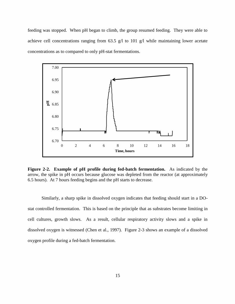
feeding was stopped. When pH began to climb, the group resumed feeding. They were able to
achieve cell concentrations ranging from 63.5 g/l to 101 g/l while maintaining lower acetate
concentrations as to compared to only pH-stat fermentations.
Figure 2-2. Example of pH profile during fed-batch fermentation. As indicated by the
arrow, the spike in pH occurs because glucose was depleted from the reactor (at approximately
6.5 hours). At 7 hours feeding begins and the pH starts to decrease.
Similarly, a sharp spike in dissolved oxygen indicates that feeding should start in a DO-
stat controlled fermentation. This is based on the principle that as substrates become limiting in
cell cultures, growth slows. As a result, cellular respiratory activity slows and a spike in
dissolved oxygen is witnessed (Chen et al., 1997). Figure 2-3 shows an example of a dissolved
oxygen profile during a fed-batch fermentation.
6.70
6.75
6.80
6.85
6.90
6.95
7.00
0 2 4 6 8 10 12 14 16 18
pH
Time, hours

16
Figure 2-3. Dissolved oxygen profile during fed-batch fermentation. The spike at
approximately six hours indicates that substrate has been depleted from the reactor (indicated by
the arrow). After feed commences at 7 hours, the dissolved oxygen concentration decreases as
growth begins to increase.
Chen et al. (1997) coupled pH and DO-stat controlled fermentations in an attempt to
optimize cell growth. Using fermentation software, Chen et al. set up a system that triggered a
feed pump every time the dissolved oxygen or pH rose above their desired set points. Similarly,
the pump was deactivated when both the dissolved oxygen and pH dropped below the set points.
They witnessed a 4-fold increase in cell concentration and improved plasmid yields 10-fold
using this method.
The last classification of feed types contains methods in which feedback is not involved
(non-feedback control). This group includes constant or pulsed feeding, increased feeding, or
exponential feeding (Lee, 1996). These methods are simple in comparison to pH-stat or DO-stat.
0
50
100
150
200
250
300
350
400
450
0 2 4 6 8 10 12 14 16 18
Dis
solv
ed o
xgy
en, p
erce
nt
Time, hours

17
pH-stat relies on detecting a tenth of a pH unit change and there can be a probe drift issue.
Similarly, for DO-stat, the probe can drift with time and cause minor fluctuations to go
unnoticed. In constant feeding, a predetermined amount of substrate is added at a constant rate
to the system. This method does not require any feedback from the reactor or take into account
any characteristics of the growth environment. Because the growth demands will eventually
overcome the amount of substrate fed, the specific growth rate decreases during cultivation.
Pulsed feeding involves adding an amount of substrate into the reactor. After this period,
substrate addition is paused and may resume at a later time. The down side of pulsed feeding is
that it can cause glucose oscillations. Lin and Neubauer (2000) found that while these
oscillations inhibit overgrowth of plasmid-free cells, they negatively affect product yield and
stability. These glucose oscillations can also be present in types of fed-batch fermentation. If
the uptake of glucose exceeds the local mass transfer of glucose, cells may be starved for a short
period of time (Neubauer et al., 1995). As discussed previously, this is especially important
when scaling-up processes because mixing may become an issue.
In increased feeding, a step-wise feeding strategy may be employed. This helps
compensate for the decrease in specific growth rate, as witnessed in a constant feeding strategy.
Lastly, a constant specific growth rate can be targeted using an exponential feeding strategy
(Lee, 1996). An exponential fed-batch fermentation method commonly used to pre-determine
the amount of glucose that should be fed into the reactor to achieve a certain growth rate was
proposed by Korz et al. and Lee et al. (Korz et al., 1995; Lee, 1996):
(2.1)
18
where Ms is the mass flow rate (g/h) of the substrate, F is the feeding rate (l/h), SF is the
concentration of the substrate in the feed (g/l), μ is the specific growth rate (1/h), represents
the biomass on substrate yield coefficient (g/g), m is the maintenance coefficient (g/g h), and X
and V represent the biomass concentration (g/l) and cultivation volume (l), respectively. The
yield coefficient for E. coli on glucose is generally taken to be 0.5 g/g. The maintenance
coefficient is often 0.025 g/g h (Korz et al., 1995). This equation has been widely adapted for
fed-batch fermentation processes, as exponential feeding allows cells to grow at a constant rate
(Kim et al., 2004).
For most fermentation experiments, the feeding strategy does not change after induction
of the protein. However, Wong et al. (1998) report on the effect of post-induction feeding
strategies. This group tested pH-stat, constant, exponential, and linearly increasing the feed after
induction occurred. They found that after induction, the dry cell weight was not a function of the
feeding strategy. Before induction, the dry cell weights did depend on the strategy employed to
add nutrients to the system. However, the amount of protein varied depending on the strategy
used after induction. This may be important to consider if production levels or growth begin to
significantly decline after induction.
2.4 Expression and production
To increase production of recombinant proteins it is important to maximize the number of
cells that can properly express the protein (Aucoin et al., 2006). This maximum production can
be inhibited by strong promoters because of the increased metabolic burden placed on the cell.
The resulting protein production can inhibit cell growth or cause cell degradation. Therefore, it
is important to separate the growth phase and the protein production phase (Aucoin et al., 2006).

19
For the control of the synthesis of the target protein, the DNA for the inducible promoter is
placed 5’ to the target protein’s genetic code (Aucoin et al., 2006). Thus, when the promoter is
induced, the production of the target protein is also triggered by the physical change in the cell’s
environment. Hence, a distinct production period occurs that can be tracked separately from a
growth period.
The solution to this problem is to use a promoter that can be induced by a chemical or
temperature change. Inducing the promoter activates the production of the desired protein. This
decreases the likelihood of proteases degrading the target protein during cell growth (or in the
case of toxic proteins, inhibiting further growth). Examples of common chemical inducers
include isopropyl-β-D-thiogalactopyranoside (IPTG), lactose, and arabinose. Some promoters
are thermally inducible, meaning that a drop or increase to a particular temperature will activate
the promoter, and hence activate the production of the target protein. For example, 30°C may be
used for a pre-induction growth temperature and the temperature may be shifted to 36 to 42° for
protein expression (Harder et al., 1993).
2.4.1 Lac operon
The lac operon is used to control therapeutic protein synthesis in the context of the work
for this dissertation. It is typically induced with IPTG, but because of its high cost and toxicity
to humans, IPTG is not desired for large scale production (Gombert and Kilikian, 1998;
Menzella et al., 2003; Neubauer et al., 1992). As an alternative, induction with lactose can cause
recombinant protein expression. A promoter that can be activated by IPTG will also be activated
in the presence of lactose, but lactose can be metabolized by cells whereas IPTG cannot. Thus,
20
after induction with IPTG, the concentration of the inducer remains constant whereas the lactose
concentration may change if it is used as an inducer.
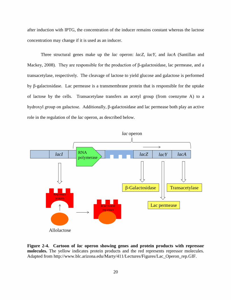
Three structural genes make up the lac operon: lacZ, lacY, and lacA (Santillan and
Mackey, 2008). They are responsible for the production of β-galactosidase, lac permease, and a
transacetylase, respectively. The cleavage of lactose to yield glucose and galactose is performed
by β-galactosidase. Lac permease is a transmembrane protein that is responsible for the uptake
of lactose by the cells. Transacetylase transfers an acetyl group (from coenzyme A) to a
hydroxyl group on galactose. Additionally, β-galactosidase and lac permease both play an active
role in the regulation of the lac operon, as described below.
Figure 2-4. Cartoon of lac operon showing genes and protein products with repressor
molecules. The yellow indicates protein products and the red represents repressor molecules.
Adapted from http://www.blc.arizona.edu/Marty/411/Lectures/Figures/Lac_Operon_rep.GIF.
lacZ lacY lacA
β-Galactosidase
Lac permease
Transacetylase
lacI RNA
polymerase
Allolactose
lac operon
Repressor
protein
Inactivated
repressor

21
Repression of the lac operon is controlled by lacI (Santillan and Mackey, 2008). Under a
different operon, lacI codes for the lac repressor. The repressor inhibits the transcription of lac
operon genes by binding an operator. This repressor is inactivated when it is bound to
allolactose (a byproduct of lactose metabolism). A positive feedback loop exists in this system
(Santillan and Mackey, 2008; Santillan and Mackey, 2008; Santillan, 2008; Santillan, 2008; van
Hoek, M. J. A. and Hogeweg, 2006; van Hoek, M. J. A. and Hogeweg, 2007). This loop gives
rise to bistability of the lac operon. Bistability occurs when there are two stable equilibria for the
operon that exist for certain inducer concentrations: induced and repressed (van Hoek, M. J. A.
and Hogeweg, 2007). As lac permease and β-galactosidase are produced, there is an increase in
the rate of lactose uptake. This in turn causes an increase in lactose metabolism which increases
the concentration of allolactose. Since allolactose decreases the activity of the repressor, there is
an increase in lac operon activity. This results in an increase in production of lac permease, β-
galactosidase, and transacetylase. A schematic of the lac operon with its repressor molecules
and protein products is given in Figure 2-4.
The lac operon can be downregulated by glucose. The concentration of extracellular
glucose effects the production of an activator that upregulates gene expression by increasing the
affinity of mRNA polymerase to the lac promoter. As the concentration of extracellular glucose
increases, the intracellular production of cyclic adenosine monophosphate (cAMP) decreases.
cAMP binds to a receptor (cAMP receptor protein) to form the CAP complex. This complex
binds DNA upstream from the lac promoter and increases the affinity of mRNA polymerase to
the lac promoter. Thus, a decrease in cAMP leads to a decrease in the CAP complex, which
causes a decrease in affinity of mRNA to the lac promoter. This phenomenon is known as

22
catabolite repression. In a separate mechanism, external glucose also decreases the efficiency of
lac permease to transport lactose into the cell (Santillan and Mackey, 2008).
2.4.2 Simple induction strategies
For simple batch cultures, the chemical inducer is typically added at the mid-exponential
growth phase of the culture. At this point, there are many cells in the culture to be induced, but
there is still opportunity for growth of new cells. Though, induction towards the end of the log
phase or during the stationary phase can affect product solubility and influence expression levels
(Berrow et al., 2006). For fed-batch experiments, the induction technique varies. Since overall
yield of the product depends on the overall biomass concentration and the product yielded from
each cell, high cell density cultivations coupled with satisfactory induction techniques should be
developed to increase overall yield (Gombert and Kilikian, 1998). In order to balance cell
growth and maintain specific cellular protein yield, the induction strategy should take the
following into account: level of gene expression, toxicity of product (either concentration of
product or the product itself), localization of the induced product, and the degradation
characteristics of the product (Tripathi et al., 2009).
There are multiple methods used to induce high cell density cultures. Some of these are
as simple as inducing at a particular optical density (similar to shake flask or batch cultivations).
Others may involve pulsing the inducer into the system at different times or adding multiple
types of inducer. An examination of specific methods follows.
Examples of simple induction methods are briefly summarized. Fan et al. (2005) induced
a high cell density culture when the OD600 reached 95 units by increasing the temperature by ten
degrees. After two hours, the temperature was decreased by three degrees. Similarly, Shin et al.
23
(1997) induced fed-batch cultivations with IPTG when the cell concentration reached 70 to 80
g/L. Kweon et al. (2001) induced a fed-batch culture with IPTG when the cell mass had reached
its highest and ended the fermentation experiment three hours later. This group also tested
protein production using different ratios of lactose and IPTG as inducers. They found that
lactose alone only produced 55% of protein that IPTG produced and increasing the ratio of IPTG
to lactose caused protein expression to increase. Another relatively simple, but unique idea was
set forth by Sandén et al. (2003). They induced fed-batch cultures at certain growth rates to
examine the effect the growth rate had on the culture. They used IPTG to induce cultures when
μ = 0.5 h-1
(during exponential feeding) or when μ = 0.1 h-1
(after they switched to constant
feeding). The group found that experiments with higher feed rates gave a higher production of
target protein.
Similar to this work, Ramchuran et al. (2005) was interested in examining lactose
induction versus IPTG induction and their effects on recombinant protein production. They
induced all cultures at the same given cell mass concentration, but varied the length of the
induction period depending on the inducer used (3 hours for IPTG, 6 hours for lactose). They
determined that lactose was a viable choice for prolonging the production phase as compared to
IPTG.
After a thorough examination of studies performed on lactose induction, it is apparent
that the optimal timing of induction is dependent on the desired product. Neubauer et al. (1992)
found that the yield of recombinant protein increased if lactose was added when the glucose
concentration was low. This group found that "lactose, when added during the transition from
the exponential to the stationary phase, can induce overexpression" of recombinant protein.

24
Interestingly, waiting an hour after this transition to induce cultures caused a decrease in their
target protein expression (Donovan et al., 1996; Neubauer et al., 1992). These experiments
showed that induction with lactose when glucose is nearly depleted is optimal for their target
protein expression. It is important to keep in mind that they did not examine induction with
lactose in a fed-batch fermentation scenario.
On the fed-batch scale, Gombert and Kilikian (1998) induced cultures with lactose 20
minutes prior to the end of the fed-batch fermentation stage. Inducing cultures this way allowed
induction to start when growth rates were still high. This group also pulsed lactose into the
system three different times after the conclusion of the fed-batch phase. In order to test
Neubauer's hypothesis about induction timing, for some experiments, the first lactose pulse was
added when glucose was depleted. For others, lactose was added 20 minutes prior to glucose
exhaustion. After comparing these two methods, a higher target protein concentration was
achieved when lactose was added prior to glucose exhaustion. They also found that residual
lactose concentrations played an important role in the decrease in yield of target protein as
increasing the amount of lactose pulsed into the fermenter (to 5.7 g/g DCW as opposed 4.3 g/g
DCW) caused a decrease in product concentration. In experiments where they added 1.2 to 2.3 g
lactose/g cell, they stated that the lactose concentration wasn't high enough to cause protein
expression. Throughout their experiments, growth did not appear to be affected by the switch
from the fed-batch phase to the induction phase, but they also pulsed yeast extract into the
system in the runs that were most successful at producing recombinant protein.
Menzella et al. (2003) also examined using lactose as an inducer for fed-batch
fermentation experiments. This group induced cells after the OD590 reached 120 units. They
25
used a pre-determined feed rate based on the substrate balance equation previously discussed to
reach that particular OD. To induce the culture, a 35% lactose solution was fed into the reactor
using a DO-stat method to avoid acetate accumulation. This method is very similar to that of
Gombert and Kilikian (1998). The Gombert group pulsed lactose into the system when they
noticed a sharp rise is dissolved oxygen. The DO-stat method of feeding lactose into the reactor
essentially feeds after the oxygen levels rise above a certain level. However, Menzella et al.
(2003) followed the feeding lactose with the feeding of a 35% glucose solution into the system.
They found that increasing the lactose concentration above 0.8 mM did not increase the amount
of protein produced. The fastest rate of lactose feeding corresponded to the highest volumetric
yield of target protein. From this, they concluded that the lactose was used both as a carbon
source and inducer very efficiently.
Hoffman et al. (1995) used a feeding medium to induce cultures with lactose on defined
media. In their experiments, the feeding solution contained 600 g/l glucose as a carbon substrate
supplemented with 50 g/l lactose for induction. Using this technique of inducing, they found that
the growth rate slowed, but that it was still higher than what they found for cultures grown on
complex media and induced with IPTG or lactose (as batch addition). The induction period
lasted for 5-12 hours and resulted in a 12-fold increase in volumetric productivity as compared to
the results they achieved for batch cultures.

26
2.4.3 Auto-induction
Another induction technique is referred to as auto-induction. According to Xu et al.
(2012), auto-induction is defined as "automatic induction of recombinant protein expression by
inducing compounds such as lactose already present in either complex or chemically defined
media at the beginning of cultivation." When the preferred carbon sources are exhausted, auto-
induction can occur. This is based on diauxic growth of cells on lactose after the preferred
carbon sources are gone. Most auto-induction mediums contain mixtures of glucose, glycerol,
and lactose (Blommel et al., 2007; Li et al., 2011). After initial consumption of glucose,
metabolism shifts to consume lactose and glycerol. Auto-induction techniques allow for the shift
from an un-induced state to an induced state to be controlled by the host organism (Blommel et
al., 2007). Auto-induction is an option with respect to this dissertation since lactose can be used
to induce the lac operon. As long as lactose is added to the media prior to the start of cultivation
or prior to depletion of the primary substrate (glucose), auto-induction of the culture will occur.
It is important to note that most strategies utilizing auto-induction require the use of yeast
extract or other undefined components. Studier (2005) published his findings on auto-induction
in 2005. In his paper, Studier reports on significant concentrations of target protein expressed
without the required inducer when cultures were grown using certain complex media. He
developed a strategy for auto-inducing shake flasks using media that contains a soluble
enzymatic digest of casein, yeast extract, and a variety of salts, minerals, and amino acids. Since
then, Studier's media recipe has been commercialized by EMD Biosciences as the "Overnight
Express Autoinduction System" (Grabski et al., 2005). This system contains three different
types of media for auto-induction of cultures, two of which are complex. The remaining type is
27
defined, but it is recommended for Se-Met labeling of proteins for further use with x-ray
crystallography studies, not necessarily for enhancing the production of protein without adding
an inducer (Grabski et al., 2005).
Auto-induction of shake flasks is a fairly straightforward procedure, as all medium
components and inducer are present at the start of cultivation. For auto-induction of fed-batch
fermentation experiments, the feeding of glucose can interfere with this induction technique. In
most fed-batch fermentation experiments, the feeding of glucose into the reactor begins as the
glucose in the media initially is consumed. This would not allow for the consumption of lactose
to occur, so perhaps induction will not take place. Also, as previously discussed, the build-up of
glucose in the media can inhibit the action of the lac operon, so induction would not occur or it
would be significantly haltered. This is where the use of an alternative feed source would come
into play. Glycerol can be used to maintain growth. Additionally, E. coli does not preferentially
consume glycerol over lactose. Thus, the lactose may have a chance at acting as an inducer once
the glucose is depleted during the batch phase.
However, a different set of batch-scale experiments by Kim et al. (2007) showed that
lactose induction results in an 8-fold increase in protein compared to auto-induction and a 20-
fold increase in yield compared to IPTG. Though, auto-induction increased yield 3-fold
compared to simple IPTG induction while also decreasing costs. First cells were grown up in
media containing glycerol as a carbon source. After depletion of glycerol, primary induction was
performed by adding IPTG and lactose to final concentrations of 1 mM IPTG and 0.2% lactose.
Six hours later, a portion of this culture was used to inoculate fresh medium containing 2%
lactose as a sole carbon source and fermentation continued for 18 hours. Glycerol was used as
28
the initial carbon source to prevent by-product formation that occurs from glucose metabolism.
Lactose was added when glycerol was depleted because they assumed that the cells would more
readily take up lactose if no other source of carbon was present and IPTG was used as a pre-
inducer to "pre-activate" the cells. They found that this IPTG/lactose primary induction method
with growth on lactose for 18 hours after induction increased the yield of protein as compared to
growth on auto-induction media or induction with IPTG alone. It is important to note that the
media this group used contained casein hydrolysate and yeast extract. These results indicate that
a simple auto-induction technique may not be sufficient when inducing high cell density
cultivation.
Work by Kotik et al. (2004) suggested that lactose pulsing with auto-induction can
increase product formation. The initial media used casein hydrolysate, salts, and lactose. They
fed the system exponentially with glycerol and supplemented the feed with one gram of lactose
every 2 hours. Volumetric productivity increased 100-fold compared to shake flasks with LB.
In their work, they conclude that "intermittent addition of lactose during fed-batch growth was
sufficient for a long-lasting and efficient production of [protein]."

29
2.5 Dynamic modeling and metabolic flux analysis
Mathematical modeling is often used to estimate and predict protein production given a
set of changing conditions. This modeling is refered to as dynamic modeling in this dissertation.
Dynamic modeling takes into account the concentration of inducer by incorporating equations
that represent how concentrations of regulatory molecules change during the induction process.
In this case, the bistability of the lac operon can be modeled using a set of differential equations
that describe the regulation of the operon. The following two equations are representative of
those that are utilized for this type of modeling (Chen et al., 1991; Cheng et al., 2001; Kremling
et al., 2001; Wong et al., 1997):
])[(][][
i
ndegradatio
ii
synthesis
i
i mRNAkGkdt
mRNAd (2.2)
jiproteinkmRNAkdt
proteindj
ndegradatio
i
synthesis
j
j
j ];)[(][
][ (2.3)
In these equations, k and µ represent rate constants for synthesis and degradation of proteins and
the specific growth rate, respectively. [mRNA], [G], and [protein] represent the concentrations of
messenger RNA, gene for repressor protein, and recombinant protein product, respectively. In
the first equation, α represents the dosing of IPTG (or lactose), since the production of
recombinant protein is IPTG dose dependent. In both equations, the first term represents the
increase in formation due to production. The second term represents the decrease in
concentration due to degradation and dilution due to growth. As the number of cells increase,
the concentration on a per cell basis decreases. Therefore, the growth rate is taken into account.
Similar mass balance equations can be written to describe cyclic-AMP, mRNA, enzyme
concentrations, and repressor RNA concentration. It is important to include all of these mass
balances because each one affects the final concentration of the target protein.
30
These equations work for batch fermentations and can potentially be used for fed-batch
cultivations. However, there is an additional set of equations that describe the growth
characteristics and by-product formation for fed-batch fermentation processes. This type of
modeling does not provide any information on production formation, but can accurately describe
other physical conditions in the fed-batch reactor. As described by many groups the equations
below represent the change in feed, volume, cell mass, acetate, and glucose that occur during the
fermentation process (Chen et al., 1995; Cockshott and Bogle, 1999; Jenzsch et al., 2006;
Levisauskas and Tekoris, 2005; Mohseni et al., 2009; Roeva et al., 2007; Roeve and Tzonkov,
2006; Xu et al., 2008). The groups also report on utilizing Monod kinetics to incorporate the
inhibition of growth by certain by-products in the growth rate term.
Volume equation:
(2.4)
Cell mass equation:
(2.5)
Acetate equation:
(2.6)
Glucose equation:
(2.7)
The feed equation that this type of model typically incorporates is the same as the
equation given in Section 2.3.3 where feed rate is based on the specific growth, feed
composition, and other constants that describe reactor conditions. The change in volume
depends on the feeding strategy and since the feed rate changes with time for exponential
feeding, the change in volume can be defined by the feed rate. In some cases, if the sample size
at a specific time is large, this size can be account for by subtracting it from the feed equation. In

31
the case of this dissertation, the volumes of the samples taken are negligible with respect to the
volume of the broth in the reactor. For constant-volume cultivations, the cell mass equation is
usually denoted by μ*X. For fed-batch experiments, dilution occurs due to the addition of
substrate. Hence, the cell mass equation for a fed-batch experiment includes a term for dilution
due to feeding/volume changes.
For changes in carbohydrate concentrations, the dilution due to volume changes is again
taken into account. For determination of acetic acid, the amount re-consumed by the cells is
subtracted from the amount generated from the cells. Since these amounts are calculated on a
per cell basis, the sum is multiplied by the cell mass. Here, the amount of acetate consumed is
represented by the Monod equation and the amount generated follows Tessier-type kinetics since
the amount generated depends on the concentration of glucose:
(2.8)
(2.9)
For glucose, the saturation constant, the maximum uptake rate, and information about
acetic acid concentrations are used to calculate the amount consumed. Since cells can consume
acetic acid, Monod-type noncompetitive inhibition kinetics is used. In the equations above, the
amount of consumed glucose is denoted by qGc, with qGc defined as follows:
(2.10)
32
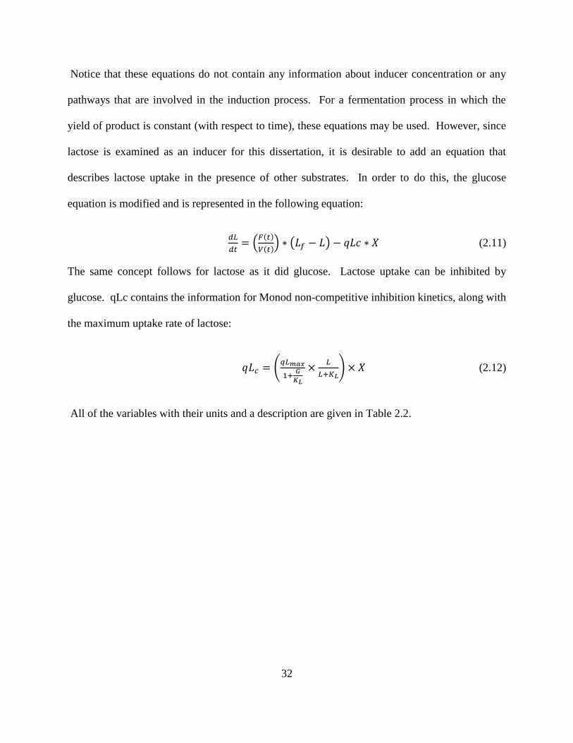
Notice that these equations do not contain any information about inducer concentration or any
pathways that are involved in the induction process. For a fermentation process in which the
yield of product is constant (with respect to time), these equations may be used. However, since
lactose is examined as an inducer for this dissertation, it is desirable to add an equation that
describes lactose uptake in the presence of other substrates. In order to do this, the glucose
equation is modified and is represented in the following equation:
(2.11)
The same concept follows for lactose as it did glucose. Lactose uptake can be inhibited by
glucose. qLc contains the information for Monod non-competitive inhibition kinetics, along with
the maximum uptake rate of lactose:
(2.12)
All of the variables with their units and a description are given in Table 2.2.

33
Table 2-2. Variables, units, and description of variables used for dynamic modeling of a
fed-batch fermentation process.
Variable Units Description
F(t) l/hr Feed rate
V(t) liter Volume
X(t) grams Cell mass
A(t) g/l Acetate concentration
G(t) g/l Glucose concentration
L(t) g/l Lactose concentration
μ 1/h Specific growth rate
Gf g/l Glucose concentration in feed
X0 grams Cell mass at time of feed start
V0 liter Volume at time of feed start
Yc/g g/g Yield of cells on glucose
qAg g/gh Acetate generated during fermentation
qAc g/gh Acetate reutilized or consumed
qGc g/gh Glucose consumption rate
Lf g/l Lactose added
qLc g/gh Lactose consumption rate
qAcmax g/gh Maximum uptake of acetate
qGcmax g/gh Maximum uptake of glucose
qLcmax g/gh Maximum uptake of lactose
KG g/l Saturation constant for glucose
KL g/l Saturation constant for lactose
KA g/l Saturation constant for acetate
KX -- Exponent fit to data for generation of acetate from glucose
It is also important to note the need for a maintenance coefficient. In most cases, the set-
point for the growth rate in the feed profile is not the growth rate that the culture achieves. This
can cause major discrepancies between the experimental observations and the simulated data.
Typically, after modeling the feed profile, volume, and cell mass, one can determine when and if
a maintenance coefficient will be needed (depending on the simulation of cell mass compared to
data obtained from the fermentation experiments).
34
While dynamic modeling examines the fed-batch system on the macro-scale, one method
commonly used to optimize E. coli production on the micro-scale is metabolic flux analysis
(MFA). Metabolic flux analysis allows for the assessment and prediction of metabolite
concentrations and rates of reactions during the cellular metabolism process using a constraints-
based approach. Knowledge is gained about how metabolic fluxes are utilized by cells and how
cells optimize their growth rates by tracking the movement of carbon throughout the system
(Varma and Palsson, 1994a). As previously discussed, in order to produce high concentrations
of bacterial cells, fermentation processes are utilized. For bacterial fermentations, the products
are typically the cells themselves, but they can also be metabolites that the cells produce during
the fermentation process. In order to tightly control this process, the medium that the cells are
grown is monitored and controlled. Glucose and other carbon sources can be added for
nutritional purposes. Additionally, since E. coli grows aerobically, the rate of oxygen into the
fermentation tank is controlled.
MFA utilizes mass and energy balance principles (Meadows et al., 2010). A substance
that is put into the system must leave the system in some form or another. The rate at which this
occurs is referred to as the pathway flux (Koffas et al., 1999). In some fermentation processes,
glucose is put into the system as a feed source. The carbon from glucose may leave the system
in the form of protein, amino acids, cellular components, or secreted products. Hence, MFA
tracks the rates at which these types of metabolites form during cellular metabolism in a
fermentation process using data about stoichiometry, cell components, and growth kinetics
(Pramanik and Keasling, 1997). Using this constraints-based approach, the objective function is
a metabolic process, such as the production of biomass (cell mass). Constraints are determined
by the underlying cellular processes that occur which may limit the behavior of a particular cell
35
and its growth rate. These constraints determine a solution space, and an objective function is
then optimized using linear programming methods. Overall, metabolic flux models incorporate
stoichiometry of metabolic pathways, requirements for growth during metabolism, and
corresponding optimality principles to predict the flux distribution and growth of the cell under
particular conditions of the cellular environment (Varma and Palsson, 1994a). After the model is
solved, it can be used to accurately describe the time course of growth and product secretion
(proteins, metabolites, cellular components), in addition to predicting the effects of eliminating
or altering genes in the bacteria’s genetic profile.
Many researchers use isotopic labelling to monitor metaoblic processes. Using these
methods, stable isotope measurements can be used to gain information about fluxes. For
example, Antoniewicz et al. (2007) used 13
C-labeled glucose for feeding cultures. After feeding
with natural glucose, they used the labeled glucose to track uptake and distribution to other
molecules. For labeled experiments, fluxes must be obtained using nuclear magnetic resonance
(NMR) or mass spectrometry (MS). Then, the data with information about fluxes and molecular
requirements can be fitted with computer modeling (Sauer, 2006). The difference between the fit
and the data is minimized to get a better description of the fluxes. However, it is not necessary
to use isotopic labeling to perform MFA on bacterial systems.
In order to use metabolic flux analysis, mass balance equations for each metabolite must
be written. The concentration of each substrate is equal to the difference between the amount
generated from the metabolic precursor and the amount used as a metabolic precursor to some
other component. Under non-steady state conditions, information about the accumulation of
metabolites must also be contained. Mathematically, this can be written as where A is
36
a matrix that contains all of the stoichiometric information, r is a vector that contains the
information about transport and reaction fluxes, and x is a vector that contains metabolite
concentration data (Covert et al., 2001). Note that A will be a large matrix comprised mostly of
zeroes and ones depending on the stoichiometry of the set of reactions that are to be modeled.
Under balanced growth conditions and due to the fact that the reactions are fast between
metabolic substrates (milliseconds to seconds) compared to growth (hours or days), the system
can be assumed to be operating under steady-state conditions. Hence, .
To minimize the number of possible solutions, many constraints can be used. For
example, the fluxes must be a positive number and since they exist in a single direction, r must
be greater than or equal to zero. Data about substrate yields can also be used to further constrain
the flux vector. Lastly, linear programming is used to optimize a desired objective. For
example, the objective may be to maximize biomass. If this is the case, then linear programming
would be used to maximize biomass with respect to the constraints defined for the fluxes and the
information contained in the stoichiometric matrix. The resultant outcome would be the actual
fluxes calculated with the biomass output.
As summarized by Stephanopoulos (1999), there are many other applications for
metabolic flux analysis:
(1) improvement of yield and productivity of products native to host
(2) production of products that are new to the host cell
(3) improvement of cellular properties (i.e. prevention of overflow metabolism or
the ability to withstand certain fermentation conditions)
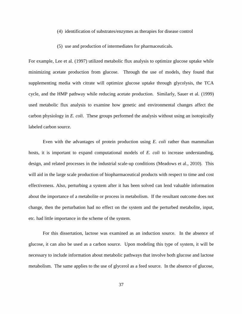
37
(4) identification of substrates/enzymes as therapies for disease control
(5) use and production of intermediates for pharmaceuticals.
For example, Lee et al. (1997) utilized metabolic flux analysis to optimize glucose uptake while
minimizing acetate production from glucose. Through the use of models, they found that
supplementing media with citrate will optimize glucose uptake through glycolysis, the TCA
cycle, and the HMP pathway while reducing acetate production. Similarly, Sauer et al. (1999)
used metabolic flux analysis to examine how genetic and environmental changes affect the
carbon physiology in E. coli. These groups performed the analysis without using an isotopically
labeled carbon source.
Even with the advantages of protein production using E. coli rather than mammalian
hosts, it is important to expand computational models of E. coli to increase understanding,
design, and related processes in the industrial scale-up conditions (Meadows et al., 2010). This
will aid in the large scale production of biopharmaceutical products with respect to time and cost
effectiveness. Also, perturbing a system after it has been solved can lend valuable information
about the importance of a metabolite or process in metabolism. If the resultant outcome does not
change, then the perturbation had no effect on the system and the perturbed metabolite, input,
etc. had little importance in the scheme of the system.
For this dissertation, lactose was examined as an induction source. In the absence of
glucose, it can also be used as a carbon source. Upon modeling this type of system, it will be
necessary to include information about metabolic pathways that involve both glucose and lactose
metabolism. The same applies to the use of glycerol as a feed source. In the absence of glucose,

38
glycerol provides the necessary source of carbon and the pathways/reactions that describe
glucose metabolism can also be incorporated into the model.
2.6 Purification
A major task for the pharmaceutical industry is to achieve highly purified and well-
characterized production of recombinant proteins (Terpe, 2003). In order to separate and purify
the target protein from the pool of proteins expressed during the fermentation process, fast
protein liquid chromatography (FPLC) is a common strategy that is utilized. The column
typically used in this system contains a cross-linked resin that has ligands attached to its surface
depending on the protein of interest. The total soluble lysate is loaded to the column. During the
loading step, the protein of interest interacts with the ligands on the surface of the resin. This
interaction causes the target protein to adsorb to the resin or causes the protein to slow its
progress through the column. After the total protein pool passes over the column, the column is
washed to elute loosely bound or contaminant proteins. Then, elution of the target protein
follows. This occurs by loading the elution buffer to the column. The buffer typically contains a
species that interferes with the binding of the target protein to the column resin. The purified
sample is then collected and further analyzed.
One type of FPLC is referred to as affinity chromatography due to the attraction between
the target protein and the biospecific surface ligands. In order to create interactions between
surface ligands and target proteins, the genes encoding for the target protein will often be
genetically altered prior to expression and production. In this process, the DNA encoding for the
additional tag or affinity tail is fused to a gene of interest. Then, when the target protein is
expressed during fermentation, the tag is expressed with it resulting in the affinity tag – target

39
protein complex. Purification tags have been used to facilitate purification in affinity, ion-
exchange, hydrophobic, covalent, and metal-chelating separations (Sassenfeld, 1990).
There are several advantages to using affinity tags to facilitate the purification of a
particular protein. Some tags can increase the solubility of the target protein and also add
stability to the protein. For some proteins, there is also a minimal effect on the tertiary structure
and the biological activity of the target protein (Terpe, 2003). The affinity tails can also allow
for simple and accurate assay of the affinity tag – target protein complex during purification
(Sassenfeld, 1990; Terpe, 2003). Affinity tails are also extremely versatile and affinity
chromatography usually results in a product that is 90-99% pure (Terpe, 2003). Tails can be
added at the N-terminus or the C-terminus of the protein and can be expressed in many different
cellular systems – bacterial, yeast, and mammalian (Terpe, 2003). One disadvantage of using
affinity tags is that the column resin often costs more than that not using a biospecific ligand.
Secondly, the fact that the protein must have a tag added on to the tail end can be a disadvantage
in some cases because removal of the tail must occur prior to any additional work.
The affinity tail of interest for this project is glutathione-S-transferase (GST). This
enzyme is 26 kDa in size. Fusion proteins with a GST tail can be purified by passing the cellular
lysate over a column containing immobilized glutathione (Terpe, 2003). In order to elute the
fusion protein, reduced glutathione is used after the total protein pool has passed through the
column. The last step to achieve a final target protein in its active, therapeutic form is to cleave
the tag from the target protein. With GST, this is performed by using thrombin or Factor Xa
(Sassenfeld, 1990; Terpe, 2003). These enzymes cleave the peptide bond between the GST tag
and the target protein.
40
Figure 2-5. A typical chromatogram for chromatography utilizing a GST-tagged protein.
A change in buffer causes the elution of target proteins by disrupting the binding affinity
between the target protein and substrates in the buffer.
2.7 Medically relevant CBD-fusions as test cases for dissertation
For the work in this dissertation, an important group of therapeutic molecules was under
investigation. Expression levels of collagen binding domain fusion proteins are low, so these
types of fusion proteins are good candidates for developing methods that increase therapeutic
protein production.
Recent investigations have shown that biomaterials play an important role in tissue
engineering (Hannachi Imen et al., 2009). In order to enhance tissue regeneration both synthetic
and biological materials have been used (Shi et al., 2011). Commonly used synthetic matrix
materials used include polypropylene and polytetrafluoroethylene (Shi et al., 2011). Though
these materials show an increase in the rate of tissue regeneration, they can cause infections and
Eluted product
Flow-through
41
adhesions because they are nonabsorbable (Shi et al., 2011). On the other hand, biological
materials that have previously been used come from donors. The issue with this is that the
materials can vary due to differences in each donor. Hence, it is a necessity to find novel
biomimetic or bioactive materials that can enhance tissue regeneration without the use of
synthetic materials and without the reliance on donors (Hannachi Imen et al., 2009). Substances
that exhibit these characteristics include growth factors. Growth factors are recognized by cells
and can activate cellular regeneration, but they cannot be delivered by ordinary drug delivery
systems because of their limited target specificity and short half lives in vivo (Nozomu et al.,
1998).
Making up approximately 30% of whole-body protein content, collagen is the most
abundant protein in mammals (Chen et al., 2010; Matsushita et al., 1998). It is the major protein
component in connective tissues and bone. Collagen has been used in tissue engineering because
of its ability to provide structural stability in addition to its ability to increase cellular attachment
(Shi et al., 2011). To overcome the complications stated above, growth factors that are to be
used as therapeutic proteins have been fused to collagen binding domains (CBD) and produced
in E. coli. This reduces both problems of specificity and short half-lives because collagen
binding domain can be used as an “anchoring unit” for in vivo applications (Toyoshima et al.,
2001). It specifically targets collagen and the resulting vehicle is a non-diffusible, longer lasting
fusion protein. It has been shown that growth factors and cell binding peptides fused to
biomaterial carriers can achieve biomolecular recognition of cells in addition to interacting with
surrounding tissues (Hannachi Imen et al., 2009). Also, after the fusion of a growth factor to
CBD, recombinant proteins exhibited collagen binding activity in addition to maintaining growth
factor activity and its concentration at the target site (Shi et al., 2011).
42
It has been found that collagenase from Clostridium histolyticum has broader substrate
specificity and can hydrolyze collagen at diverse sites (Toyoshima et al., 2001). This suggests
that utilizing CBD from this source would have broader clinical applications. In designing a
CBD fusion protein it is important to keep in mind that only proteins that act in or from the
extracellular space can be used as the functional domain. Thus, the product may have to be
directly injected into affected tissue or used as an ointment (Nozomu et al., 1998).
2.7.1 PTH-CBD
Parathyroid hormone (PTH) or parathyroid hormone related peptide (PTHrP) has the
ability to increase bone density after administration (Liu et al., 2007). Hyperparathyroidism is
correlated with bone loss because of its ability to remove calcium from bones to maintain
extracellular calcium concentrations. According to Fu et al. (2005), "PTH has an anabolic effect
on bone formation by stimulating renal calcium readsorption, phosphate excretion, and bone
remodeling." Administration of PTH actually has the ability to enhance bone density (Sakon et
al., 2010). The hormone binds to receptors on osteoblasts. This action increases the longevity of
osteoblast activity, thus causing bone gain.
Parathyroid hormone also enhances epidermal cell proliferation, which can promote hair
growth. However, because of its short half-life (approximately 4 minutes), an anchoring unit
such as CBD is necessary for delivery of PTH to target cells. Indeed, a PTH-CBD fusion protein
can be used to promote bone and hair growth and to prevent cancer metastasis to bone among
other things (Sakon et al., 2010). This action is shown in Figure 2-6.
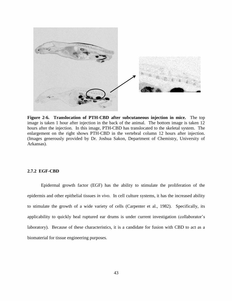
43
Figure 2-6. Translocation of PTH-CBD after subcutaneous injection in mice. The top
image is taken 1 hour after injection in the back of the animal. The bottom image is taken 12
hours after the injection. In this image, PTH-CBD has translocated to the skeletal system. The
enlargement on the right shows PTH-CBD in the vertebral column 12 hours after injection.
(Images generously provided by Dr. Joshua Sakon, Department of Chemistry, University of
Arkansas).
2.7.2 EGF-CBD
Epidermal growth factor (EGF) has the ability to stimulate the proliferation of the
epidermis and other epithelial tissues in vivo. In cell culture systems, it has the increased ability
to stimulate the growth of a wide variety of cells (Carpenter et al., 1982). Specifically, its
applicability to quickly heal ruptured ear drums is under current investigation (collaborator’s
laboratory). Because of these characteristics, it is a candidate for fusion with CBD to act as a
biomaterial for tissue engineering purposes.
44
3. Specific aims
This dissertation seeks to address important aspects of bioprocessing, namely the
expression, production, and purification methods of novel therapeutic proteins through
experiments that combine fermentation, purification, and metabolic flux analysis techniques. A
novel therapeutic protein, parathyroid hormone fused to collagen binding domain, has been of
recent interest due to its applications for therapeutic purposes. The collagen binding domain
(CBD) allows for efficient uptake of parathyroid hormone. The effects of this uptake include
decreased hair loss and decreasing losses in bone density, thus reversing or subduing the side
effects of current cancer treatments (chemotherapy). In order to enhance purification of PTH-
CBD, a glutathione S-transferase tail is attached to the PTH-CBD complex. This allows for
easier purification of the protein complex using affinity chromatography. Metabolic flux
analysis is used to model the system and the chemical induction of the therapeutic protein
complex. This aids in the development of media and induction strategies
The broad goal of this experimental program was to gather information on production of
PTH-CBD in a manner in which scale-up work is plausible in order to increase availability of the
protein complex for therapeutic purposes. This involved investigating defined mediums that
allow for high cell density cultivations while increasing protein expression, monitoring induction
techniques that will incorporate good manufacturing practice applications, and investigating
certain aspects of GST affinity chromatography. An overview of the direction of experiments is
given in Figure 3-1, with specific aims given below.

45
Specific objectives include the following scientific aims:
Aim 1. Increase expression of PTH-CBD by modifying and testing mediums appropriate to fed-
batch fermentation processes.
Aim 2. Test various induction techniques to further enhance expression of the therapeutic
protein.
Aim 3. Investigate the use of fast protein liquid chromatography with a glutathione-S-transferase
(GST) affinity column for the purification and recovery of the therapeutic protein.
Aim 4. Mathematically model the cellular system using techniques consistent with metabolic
flux analysis.
Figure 3-1. Flow chart of how experiments proceeded.
The work in this dissertation lays the foundation for increasing production of therapeutic
proteins by investigating fed-batch fermentation, media enhancement, induction techniques, and
GST purification. Such advances are of great interest to the pharmaceutical and biotechnology
Glycerol fed-
batch with
lactose
Glucose fed-batch
with lactose
Shake flask
induction
with lactose
Fed-batch
media check
Shake flask
induction
with IPTG
Media
development
(shake flasks)
3 L batch
scale media
check
Fed-batch with
lactose induction
Fed-batch with
IPTG induction
Modeling and
Purification
46
industries due to the increase in recombinant protein expression and use thereof in therapeutic
applications.
It also thoroughly examines the use of lactose as an alternative to IPTG as an inducer.
The body of literature for IPTG induction is far more mature than that for lactose. Within the
literature for lactose induction, fed-batch fermentation with lactose is rarely discussed. A search
of fed-batch fermentation "IPTG induction" within Google Scholar yields 629 results,
whereas the search with "lactose induction" yields 94 results. It is also difficult to find work on
lactose induction with fed-batch fermentation utilizing completely defined media.
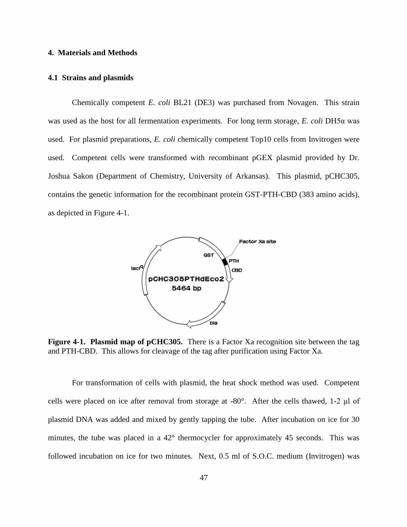
47
4. Materials and Methods
4.1 Strains and plasmids
Chemically competent E. coli BL21 (DE3) was purchased from Novagen. This strain
was used as the host for all fermentation experiments. For long term storage, E. coli DH5α was
used. For plasmid preparations, E. coli chemically competent Top10 cells from Invitrogen were
used. Competent cells were transformed with recombinant pGEX plasmid provided by Dr.
Joshua Sakon (Department of Chemistry, University of Arkansas). This plasmid, pCHC305,
contains the genetic information for the recombinant protein GST-PTH-CBD (383 amino acids),
as depicted in Figure 4-1.
Figure 4-1. Plasmid map of pCHC305. There is a Factor Xa recognition site between the tag
and PTH-CBD. This allows for cleavage of the tag after purification using Factor Xa.
For transformation of cells with plasmid, the heat shock method was used. Competent
cells were placed on ice after removal from storage at -80°. After the cells thawed, 1-2 μl of
plasmid DNA was added and mixed by gently tapping the tube. After incubation on ice for 30
minutes, the tube was placed in a 42° thermocycler for approximately 45 seconds. This was
followed incubation on ice for two minutes. Next, 0.5 ml of S.O.C. medium (Invitrogen) was

48
added to the tube. It is comprised of (per liter): 20 g tryptone, 5 g yeast extract, 10 mM NaCl, 2.5
mM KCl, 10 mM MgCl2, 10 mM MgSO4, 20 mM glucose. The cells were incubated at 37° for
three hours at 200 rpm. Cells were then spread on Luria-Bertani (LB) plates supplemented with
150 μg/ml ampicillin and incubated overnight at 37°. After colony formation, colonies were
picked for fermentation experiments and for storage in glycerol at -20° and -80°.
4.2 Media
LB was used for all plates and seed cultivations. For seed cultivations, a colony was
picked off of a plate and put in a 5 ml falcon tube containing LB and 150 μg/ml ampicillin.
These were incubated overnight at 37° and shaken at 250 rpm. Since it was desired to use a
completely defined media for fed-batch cultivations, modified minimal salts (M9) media was
investigated and compared to LB with respect to growth and recombinant protein production. As
described by Babaeipour, et al. (2008), the composition of M9 per liter of water is as follows: 10
g glucose, 15 g of K2HP04, 7.5 g of KH2P04, 2 g of citric acid, 2.5 g of (NH4)2S04, 2 g of
MgSO4-7H20, and 1 ml of trace element solution. A 5X stock was made of the salts solution.
The trace element solution contains, per liter of 1 M hydrochloric acid, the following: 2.8 g of
FeSO4-7H20, 2 g of MnCl2-4H20, 2.8 g of CoCl2-7H20, 1.5 g of CaCl2-2H20, 0.2 g of CuCl2-
2H20, and 0.3 g of ZnSO4-7H20. Glucose solutions and trace element solutions were sterilized
separately and added to the final 1X media.
4.3 Shake flask cultivations
For experiments performed in 250 ml shake flasks, 50 ml of media were inoculated with
5 ml of overnight seed culture. For 1 L shake flasks, 250 ml of media were inoculated with 20
ml overnight seed culture. Media were supplemented with 150 μg/ml ampicillin in every shake
49
flask experiment. In shake flasks that were induced, the inducer (isopropyl-beta-D-
thiogalactospyranoside (IPTG) or lactose) was added at the mid-exponential phase of growth (at
an optical density (OD) between 0.6 and 0.8 units (at 600 nm). Samples were taken throughout
the fermentation process to track protein expression and growth (via OD600).
In order to find an optimal medium for the production of recombinant protein, a number
of experiments were performed to test different media conditions. To examine the effect of
glucose on growth and protein expression, a set of flasks containing only LB was compared to a
set of flasks containing LB supplemented with 10 g/l glucose. Each flask was inoculated with
the same volume of overnight seed culture. Samples were taken every hour to track growth and
protein expression.
A similar experiment was performed to compare E. coli growth and protein expression on
M9 medium, M9 medium supplemented with amino acids, and LB. The amino acids chosen to
supplement M9 were not arbitrarily chosen, but calculated using a basis of one gram of target
protein produced. The frequency of a particular amino acid in the primary sequence can be used
to calculate the overall concentration of that particular amino acid in the protein. Using this
information, the amount of a particular amino acid required for the production of one gram of
recombinant protein can be calculated, as shown in Table 4-1. Based on the higher amounts of
lysine, aspartic acid, glycine, and leucine required, the medium was supplemented with these
amino acids. It was also supplemented with serine because serine has the ability to produce
other amino acids during metabolism. Amino acids were solubilized in water and filter
sterilized. 250 mM each of lysine, glycine, and serine were kept as stock solutions. Leucine

50
and aspartic acid stocks were 125 mM and 50 mM, respectively. Cultures were induced with
lactose or IPTG.
Table 4-1. Amino acid composition of GST-PTH-CBD with the amount of each required to
make one gram of protein.
To determine the an optimal amount of amino acids that should be added to the M9,
experiments were performed that compared the addition of amino acids to a final concentration
of 5 mM and 10 mM. Ammonium hydroxide was utilized to pH the M9 modified with amino
acids (as the amino acids dropped the pH below the physiological value). The approximate pH
for shake flask experiments was 6.8.
Ala A 89 15 3.92 1335 0.342
Arg R 174 15 3.92 2610 0.342
Asn N 132 18 4.70 2376 0.410
Asp D 133 27 7.05 3591 0.615
Cys C 121 4 1.04 484 0.091
Gln Q 146 9 2.35 1314 0.205
Glu E 147 27 7.05 3969 0.615
Gly G 75 31 8.09 2325 0.706
His H 155 10 2.61 1550 0.228
Ile I 131 26 6.79 3406 0.592
Leu L 131 36 9.40 4716 0.820
Lys K 146 31 8.09 4526 0.706
Met M 149 13 3.39 1937 0.296
Phe F 165 13 3.39 2145 0.296
Pro P 115 22 5.74 2530 0.501
Ser S 105 21 5.48 2205 0.478
Thr T 119 13 3.39 1547 0.296
Trp W 204 6 1.57 1224 0.137
Tyr Y 181 25 6.53 4525 0.570
Val V 117 21 5.48 2457 0.478
Total: 383 100 50772
382 6876
43896
Monomer
Number of peptide bonds:
0.056
mmol/g proteinMassPercentageFrequencyMW
0.058
0.050
0.035
0.028
0.103
Protein molecular weight:
Grams of aa reqd for 1
gram of protein
0.030
0.059
0.054
0.082
0.011
0.030
0.090
0.053
0.035
0.078
0.107
0.103
0.044
0.049
51
To track the consumption of glucose and lactose, 1 liter shake flasks with M9 modified
with amino acids, 10 g glucose, and 10 g lactose were inoculated with seed cultures as described
above. Samples were taken throughout the cultivation and supernatants were saved for later
analysis.
4.4 Batch cultivations
In order to further test the medium formulation prior to fed-batch fermentation, batch
fermentation was utilized. M9 supplemented with glucose and amino acids was used for all
batch fermentation experiments. No substrates were added to the media during cultivation with
the exception of ammonium hydroxide for pH control and inducer. IPTG, lactose, and a
combination of the two were used. The goal of the batch cultivations was to monitor growth
under different inducer substrates. For IPTG induction, 10mM IPTG was used. For lactose
induction, 15 grams of lactose was added per liter of medium. For induction using both lactose
and IPTG, 5 mM ITPG was used with 7.5 g/l lactose. Appropriate amounts of ampicillin and
anti-foam were added to the medium prior to cultivation.
To prepare for the fermentation process, a single colony of E. coli BL21 pCHC305 was
transferred from a plate to a 5 ml culture tube. After overnight growth in a 37° C incubator, 100
ml of M9 medium were inoculated. After six to eight hours, the 100 ml culture was spun-down
at 4750 rpm for 25 minutes and resuspended in 50 ml of fresh M9 medium. This was used to
inoculate 1 liter of medium (as previously described) in a 3 L Applikon bioreactor (Foster City,
CA). The bioreactor was equipped with BioXpert Advisory software from Applikon. The
reactor was also outfitted with an Applisense pH probe and dissolved oxygen probe. The pH
was maintained at approximately 6.8 (with a range of 6.75 to 7) during the cultivation using 7 M

52
NH4OH. The culture was stirred at 750 rpm until it became necessary to adjust the stir rate (to
1000 rpm) to maintain the proper dissolved oxygen concentration. Adjustments in oxygen
delivery were made as necessary during the process to ensure that the dissolved oxygen
concentration did not drop below 35%. The temperature was maintained at 37° C using a
heating jacket and cooling loop. Optical densities were monitored using a Bugeye optical
density probe (BugLab, Foster City, CA) and a DU800 Beckman Coulter spectrophotometer
(Brea, CA). A linear correlation for the Bugeye response to the actual OD as measured by the
spectrophotometer was determined for each individual experiment. Figure 4.2 shows a few
examples of these linear correlations.
4.5 Fed-batch cultivations
After shake flask and batch cultivations were performed to select an appropriate medium,
fed-batch fermentations were run. M9 supplemented with 5 mM amino acids and 10 mg/l
thiamine was used for fed-batch fermentation runs. This was also supplemented with 1 ml anti-
foam to control foaming and 150 μg/ml ampicillin to maintain selection. Additional anti-foam
was added during cultivation when the foam reached a level approximately 2 inches from the top
of the reactor. Unless specified, the feed for all fed-batch fermentation experiments was
comprised of the following, per liter water: 500 g glucose, 20 g MgSO4-7H20, and 5 ml trace
element solution. The glucose solution and salt solution were sterilized separately. The reactor
was outfitted as described in Section 4.4.

53
Figure 4-2. Linear correlations between optical density and Bugeye output are used to
determine the growth curve for the entire fermentation experiment in terms of optical
density. A conversion factor between optical density and dry cell weight is used to calculate the
grams of cells produced during the experiment. The average R2 value for the correlation
between the OD and Bugeye output is 0.98.
Each fermentation experiment can be broken down into a batch phase and a feeding
phase. In the batch phase, the culture used only the carbon sources provided in the medium at
the start of the cultivation. During this phase, no nutrients were fed to the reactor. After
approximately 7 - 8 hours, the feeding phase began. The exact timing depended on the lag phase
of the culture and how quickly the culture grows on the initial carbon substrate. As previously
described, a rise in pH indicated that there is no carbon present in the system. Similarly, a sharp
decline in oxygen indicated that feeding should start. In the fed-batch experiments, these two
events occurred at the same time and were witnessed by the Applikon advisory software. After
0
20
40
60
80
100
120
0 10 20 30 40 50 60
Bu
gey
e R
ead
ing
, a
rbit
rary
un
its
Optical Density, 600 nm
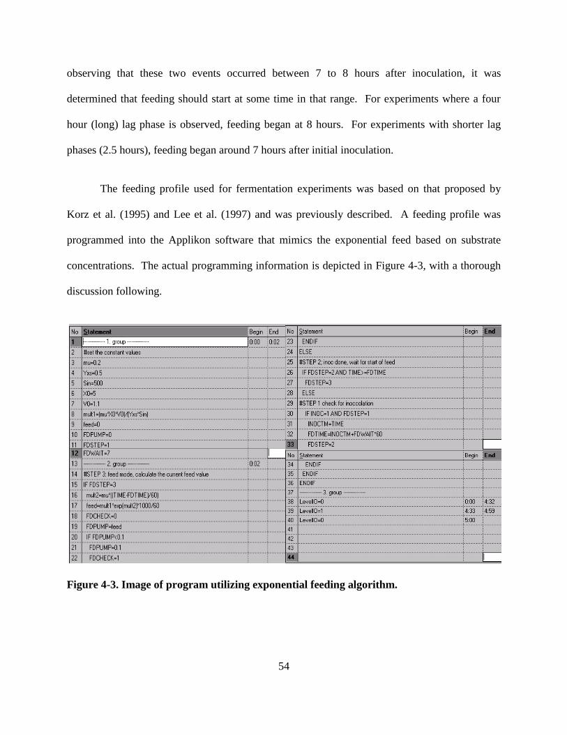
54
observing that these two events occurred between 7 to 8 hours after inoculation, it was
determined that feeding should start at some time in that range. For experiments where a four
hour (long) lag phase is observed, feeding began at 8 hours. For experiments with shorter lag
phases (2.5 hours), feeding began around 7 hours after initial inoculation.
The feeding profile used for fermentation experiments was based on that proposed by
Korz et al. (1995) and Lee et al. (1997) and was previously described. A feeding profile was
programmed into the Applikon software that mimics the exponential feed based on substrate
concentrations. The actual programming information is depicted in Figure 4-3, with a thorough
discussion following.
Figure 4-3. Image of program utilizing exponential feeding algorithm.

55
For this program, there were three separate groups of information. The program ran the
information in group one during the first two minutes of the fermentation experiment. This
essentially set the initial conditions. In lines three through 7 in the example given above, the
conditions were set to run an exponential feeding profile: μ = 0.2 hr-1
, Yx/s = 0.5 g/g, Sin = 500
g/liter, X0 = 5 g DCW, and V0 = 1.1 liters. Line 8 describes the coefficient for the feed rate
equation:
(4.1)
The only term that depends on time is the exponential term. Thus, the rest of the equation can be
calculated at the beginning of the run, as these values will not change. This coefficient was
defined as mult1 in the program. Lines 9 and 10 set the initial conditions for the feed - start at
flow rate of 0 ml/min. The FDSTEP term in line 11 set the step for the feed program - start at
step one. FDWAIT in line 12 told the program how long to wait before feed should start. In this
case, feed started after 7 hours of wait (batch) time. The second group starts on line 15, but the
first step of the second group starts on line 29. This portion of the program ran from two minutes
after the start of the experiment to the end of the fermentation run. Step 1 of group 2 identifies
that inoculation has been performed. If inoculation has been performed (based on an offline
variable that the user defines) and if the feed step is set to step 1, then the program calculated the
exact time that the feed should start. For this example, feed started after 422 minutes because the
inoculation variable was triggered after 2 minutes and the user defined FDWAIT as 7 hours.
Then, the program advanced to feed step 2 (line 22). Step 2 of the program waited until the run
time of the fermentation exceeded the 422 minutes that was calculated in step 1. After the
program time exceeded the FDTIME, step 3 commenced (on line 15). Step 3 of group 2

56
performed all of the calculations for the feeding amount of this program. Mult2 calculated the
value in the exponential term. It took into account the elapsed time and the user-defined growth
rate. In line 17, the program compiled data from mult1 and mult2 to get a feed rate in terms of
ml/min.
The system utilized a variable-speed pump to exponentially add substrate to the fermenter
at a constant rate per minute (since the program calculates an amount to feed every minute). The
minimum amount that the Masterflex® pump could add to the system is 0.1 ml/min (using the
tubing with the smallest diameter available). Lines 20 through 22 of the program accounted for
the pump sensitivity issue. If the program calculated a feed rate lower than 0.1 ml/min, the
profile corrected for this and 0.1 ml/min was actually fed into the reactor. This check was in
place until the program calculated a feed rate greater than 0.1 ml/min. This means that the
substrate was fed on a constant-feed system for about 4 hours at the beginning of the fed-batch
period. After this constant-feeding period, exponential feeding began.
The third and final group in the example program contains the information that triggered
a built-in pump. Once activated, inducer was added to the system. It turned on and turns off at
user-defined times. A value of zero indicates that the pump was turned off for that given period
while a value of 1 indicates that the pump was on. In the example in Figure 4-3, the level pump
was turned on when the elapsed time was 4 hours and 33 minutes and remained on until 4 hours
and 59 minutes.
To maintain that this feeding strategy kept the cultivation substrate limited, the
exponential feeding profile was initially regulated so that feeding stayed between 0.1 and 0.3
ml/min. For this particular experiment everything in the profile algorithm remained the same,

57
with the exception of a regulatory loop. As shown in Figure 4-4, once the algorithm calculated
that the feed should be a value greater than 0.3 ml/min, this value was divided by 0.3 so that the
value fed into the reactor returned to 0.1 ml/min. Once the calculated value exceeded 0.9
ml/min, it was divided by 0.9 to again return it to 0.1 ml/min. This regulatory group is written in
lines 24-32 in the algorithm. After the initial experiment using this profile, all other feeding
experiments used the exponential feeding algorithm that was previously described.
Figure 4-4. Image of program utilizing regulatory algorithm to keep feed rates below 0.3
ml/min during the fermentation process.

58
To examine an alternative feeding method, glycerol feed was used for a few experiments.
The media composition (M9 with amino acids) was kept the same with the exception of the
addition of 2 g/l glycerol to prime the cultivations for feed on glycerol or in the case of auto-
induction, as described below. The molar concentration of carbon in the glycerol feed was the
same as that in the glucose feed and the feed profile was kept the same. All other component
concentrations (trace elements, magnesium salts) were also kept the same. Some of these
cultivations were auto-induced and 10 g/l of lactose was added to the initial cultivation media.
One set of experiments examined using 15 g lactose to induce the culture 12 hours after
inoculation (5 hours after feeding on glycerol). Another set examined auto-induction with
pulsing 10 g lactose into the system 14 hours after inoculation (when initial lactose is depleted).
Fermenter cultivations that were not auto-induced were induced with lactose or IPTG.
For experiments in which lactose was added at the time of feed start, the level pump on the
Applikon system was utilized. By adding a couple of lines to the feed profile, the level pump
can be turned on or off at a designated time (previously discussed). The appropriate amount of
lactose was solubilized in 50-60 ml of milliQ water (to inhibit crystallization) and filter
sterilized. The solution was placed in a sterile bottle and attached to the reactor with the
appropriate tubing. The level pump was programmed to be equal to one for a thirty minute
period at the time that was desired for induction. A value of one turns the pump on; a value of
zero returns the pump to the off state. For IPTG-induced cultures, a 250 mM stock of IPTG was
made and kept in a -20 freezer until use. Final concentrations of IPTG in the reactor for
induction were 5 mM and 10 mM.

59
Multiple fed-batch experiments were performed. Table 4-2 displays the induction
technique, with respect to inducer concentration, type, and time or indicator for induction. Each
fermentation experiment was run until there was a decrease in growth or until a specified time
after induction. They typically lasted for approximately 24 hours. Samples were taken
throughout the run at specified times. The culture broth was spun down for 35 minutes at 4750
rpm and 2° C. Supernatants were filtered and stored at -20° C. Cell pellets were also stored at -
20° C.
Table 4-2. Summary of fed-batch fermentation experiments with respect to induction type,
concentration of inducer, length of induction period, and feed type. Duplicates of each run
were performed, unless specified by an asterisk.
Type of
inducer
Concentration
of inducer
Induction time or indicator Length of
induction, hours
Feed
Lactose 10 g/l 11 hours after inoculation 14 glucose (st)
Lactose 10 g/l 12 hours after inoculation 12 glucose
Lactose* 10 g/l auto-induction 25 glucose
Lactose 10 g/l at time of feed start 12 glucose
Lactose 10 + 10 g/l auto-induction with pulse at 12
hours
22 + 10 glucose
IPTG 5 mM OD ≈ 65 5 glucose
IPTG 10 mM OD ≈ 65 5 glucose
Lactose 10 g/l auto-induction 21 glycerol
Lactose 15 g/l induction at time of feed start 10 glycerol
Lactose* 10 + 10 g/l auto-induction with pulse at 14
hours
21 + 7 glycerol
4.6 Lysate preparation
Cell pellets were retrieved from the freezer and placed on ice. For pellets from 5 ml of
culture broth, 2 ml phosphate buffered saline (PBS: 8 g NaCl, 0.2 g KCl, 1.44 g Na2HPO4, 0.24 g
KH2PO4 in 1 liter) with 5 mM ethylenediaminetetraacetic acid (EDTA) was used to resuspend
the pellet. The ratio of PBS to pellet (determined by culture volume) was kept constant. After
60
resuspension in buffer, cells were lysed via sonication and spun down at 4750 rpm for 35
minutes. Lysates were stored at -20° C.
4.7 Analytical Assays
4.7.1 Cell growth and fermentation conditions
As previously discussed, cell growth was monitored using an online optical density probe
and a spectrophotometer (at 600 nm). To determine dry cell weight, analysis was performed
throughout the fermentation experiments using a Mettler-Toledo MJ33 moisture analyzer. One
ml of culture broth was spun down at 14000xg for 2 minutes. The pellet was washed twice with
milliQ water and pipetted onto the moisture analyzer. Samples were dried at 60° C until constant
weight was achieved. Calibrations were made between optical densities (taken by the
spectrophotometer) and dry cell weights. Wet cell weights were taken by either spinning down
the entire culture for 1.5 hours at 4750xg and weighing cell mass or by pre-weighing 50 ml
culture tubes. A given amount of culture was pipetted into the tube and spun down. The
difference in the weight of the tube before and after centrifugation was divided by the volume of
broth in the tube to get weight per volume (g/ml). Final volumes of culture were known, so total
weight could be calculated. Fermentation conditions such as dissolved oxygen concentration,
pH, stir rate, and temperature were monitored and logged by the Applikon advisory software
program.
4.7.2 Carbohydrate determination
Glucose concentrations were determined using a glucose hexokinase kit (Sigma, St.
Louis, MO). Acetic acid concentrations were determined using an enzyme-based kit by

61
Boehringer Mannheim/R-biopharm (Darmstadt, Germany). To determine lactose and glycerol
concentrations, a Waters high pressure liquid chromatography unit was used. Samples were
loaded onto a BioRad Aminex HPX-87N carbohydrate column at a flow rate of 1 ml/min, with
milliQ water as the mobile phase. Standards of lactose and glycerol were also loaded to
determine elution times, and to determine the peak area that corresponds with the standard
concentrations.
4.7.3 Protein analysis
Total protein concentration was determined using a Bio-Rad DC™ protein assay kit, with
bovine serum albumin (BSA) as a standard. Target protein concentrations were determined
using the densitometry technique with sodium dodecyl sulfate-polyacrylamide gel
electrophoresis (SDS-PAGE). Standards and samples were mixed with 5X sample buffer (9 ml 8
M urea, 0.242 g Tris-HCl, 0.8 g SDS, bromophenol blue (pH = 8)). Equal concentrations of
protein were loaded into the wells of a 12.5% SDS-PAGE gel. Gels were run at a constant
voltage of 250 V for 35-40 minutes, depending on the migration of the ladder marker. After
completion, gels were incubated with staining solution (250 ml methanol, 0.055 g Commassie
Blue, 250 ml de-ionized water, 50 ml acetic acid) and left overnight on a shaker. After staining
period, gels were de-stained with de-staining solution (850 ml de-ionized water, 75 ml acetic
acid, 75 ml methanol). Following the de-staining process, gels were photographed or scanned
and densitometry was performed using ImageJ software. An example of this process is given in
Figure 4-5. On the top left is a representative gel with a molecular weight ladder and three
different concentrations of BSA. Using the ImageJ software, each rectangular lane is selected
and plotted. The resultant plot is given on the right hand side. Each peak corresponds to a band

62
on the gel. Then, the peak can be selected and ImageJ will calculate the area under the curve.
The outcome for this example is shown on the bottom left side. Peak areas obtained for proteins
in lysates were compared to those obtained for BSA standards. Typical coefficients of
determination (R2) for BSA standards and peak areas were greater than 0.98.
Figure 4-5. Analysis of SDS-PAGE gel using densitometry. The coefficient of determination
for the trend between BSA concentration and peak area is 0.99.
To qualitatively compare target protein concentrations between samples, western blotting
was performed. Samples were analyzed on 12.5% SDS-PAGE gels and immunoblotted using
antibodies specific to GST. For western blotting, Protran BA 85 nitrocellulose membranes were
used (Whatman, Piscataway, NJ). After soaking western blot papers and sponges in cold towbin
buffer, transfer occurred at 100 V, constant 350 mA, for 70 minutes using a Bio-Rad transfer
apparatus. The primary antibody, polyclonal anti-GST antibody (GE Healthcare, Piscataway,
NJ), was incubated overnight at 4°C with the membrane after transfer. The secondary antibody
ImageJ Plot
ImageJ Results
63
utilized was anti-goat IgG (whole molecule) alkaline phosphatase (Sigma, St. Louis, MO). After
three hour incubation period at 4°C, visualization procedure was performed. Visualization was
completed using nitroblue tetrazolium (NBT) and 5-bromo-4-chloro-indolyl phosphate (BCIP)
until protein bands appeared.
4.8 Fast protein liquid chromatography (FPLC)
Cellular lysates were purified using a FPLC system from ӒKTA Amersham Pharmacia
Biotech. Prior to purification, cell lysates were filtered through a 0.20 μm filter. GSTrap FF
columns from GE Healthcare (Piscataway, NJ) were equilibrated with PBS loading and binding
buffer, pH=7.3. Lysates were loaded at 0.5 ml/min. Washing after loading was performed at a
flow rate of 1 ml/min with PBS. After 5 to 10 column volumes (CV) of washing (until the
baseline returned to zero), elution using 50 mM Tris-HCl with 10 mM reduced glutathione was
performed. If a peak was absent, the concentration of reduced glutathione was increased to 25
mM. Fractions were collected and stored at -20° C for further analysis.
4.9 Activity analysis
In order to assess the activity of the collagen binding domain, purified GST-PTH-CBD
was incubated for thirty minutes at room temperature on a collagen sheet. For control
experiments, green fluorescent protein (GFP) and PBS were incubated on separate collagen
sheets. After brief washing period with Towbin buffer (without methanol), the binding of GST-
PTH-CBD and/or GFP to the collagen sheets was visualized using the western blot protocol.
The primary antibody was incubated for an overnight period. The secondary antibody was
incubated with the collagen sheet for three hours. The secondary antibody was visualized using

64
NBT and BCIP, as described previously for a pre-determined amount of time as to reduce over-
development of the sheet.
4.10 Dynamic modeling
For reasons discussed in Section 6.1, it was decided that the following equations would
be used to dynamically model the fed-batch fermentation system (refer to Table 2-2 for the
description of variables):
(4.2)
(4.3)
(4.4)
(4.5)
(4.6)
(4.7)
These equations are representative of the fed-batch fermentation system with respect to feed,
volume, cell mass, acetate, glucose, and lactose. MATLAB was also used to solve this system of
equations. The values for the saturation constants were not known, so an initial guess was used.
Then, the program was designed so that MATLAB would reduce the least squares difference
between the experimentally determined measureables and the simulation output. This difference

65
was minimized by changing the saturation constants. In MATLAB, this routine was performed
using the 'fminsearch' built-in function. To simulate the system of differential equations, the
built-in ordinary differential equation (ODE) solver ODE15s was used. There are a number of
different solvers built-in to MATLAB and this particular solver is efficient at solving stiff
systems (where one component has an extremely small time step). The MATLAB code for this
model is provided in Section 9.7.
After solving this initial system, other equations were examined to model acetate,
glucose, and lactose in an attempt to obtain a better description of the relationship between these
three variables. For acetate, the following equations were examined in addition to the equation
above:
(4.8)
(4.9)
Equation 4.8 is one that is typically used in the literature to model acetic acid concentrations for
fed-batch fermentation (Mohseni et al., 2009; Roeva et al., 2007). However, this equation does
not take into account the possibility of the re-consumption of acetic acid when other carbon
sources become limiting. In this case, acetic acid is constantly excreted from the cells (given by
YA/X). Due to the widespread nature of this equation occurring in reported models for fed-batch
fermentation, it was decided to examine its usage in the context of this dissertation. Equation 4.9
is similar to the original equation proposed in the initial model. However, it no longer contains
the exponent for Tessier-type kinetics, but it still contains information about glucose and the
effect that glucose may have on acetate production.

66
For glucose, two equations were used, where the previous equation took into account the
decrease in glucose uptake due to the presence of acetate:
(4.10)
(4.11)
Equation 4.10 takes into account the addition of glucose into the reactor due to feeding and
subtracts the amount of glucose that is consumed by the cells (YS/X). However, this equation
assumes that consumption of glucose (yield of cells from substrate) is constant throughout the
entire fermentation process. It also does not take into account the presence and consumption of
other carbohydrates. Equation 4.11 follows the same Monod-type equation, but in this equation,
it is assumed that acetate does not affect glucose uptake.
For lactose, one additional equation was examined:
(4.12)
Equation 4.12 mirrors Equation 4.11, but for lactose consumption instead of glucose
consumption. The underlying assumption in this equation is that lactose is not affected by
glucose concentrations.
A combination of these equations was used in an attempt to “optimize” the model for the
fed-batch experiments performed. A number of iterations of the simulation were performed to
gain a better understanding of the relationship between the carbohydrates and their saturation
coefficients.
67
4.11 Metabolic flux analysis
As discussed in Section 2.5, metabolic flux analysis is used to gain access to information
about the processes that occur within the cell by tracking the movement of carbon throughout the
system. For the system examined in this dissertation, the pathways of three major metabolic
processes were examined: glycolysis, tricarboxylic acid cycle, and hexose monophosphate
pathway (Figure 4-6). The incorporation of lactose and glycerol into the system was also
considered (Figures 4-7 and 4-8).
A balance equation can be written for each component in the system. For example, for
the metabolic map given in Figure 4-6, the balance around glucose 6-phosphate can be written as
x2 = r1 + r33 – r2 – r3 – r4. Here, x2 represents glucose 6-phosphate, r1 and r33 both feed into
glucose 6-phosphate from glucose and lactose, respectively, and r2, r3, and r4 all pull from
glucose 6-phosphate (hence the subtraction from the overall concentration of glucose 6-
phosphate). This information can be compiled into matrix form where each balance equation
represents a row in the matrix. Mathematically, all information about the system can be written
in the form of where A is a matrix that contains all of the stoichiometric information, r
is a vector that contains the information about transport and reaction fluxes, and x is a vector that
contains metabolite concentration data (Covert et al., 2001).
It is important to note that a couple of assumptions have been made about the system.
First of all, it is assumed that all intermediates exist in a "pseudo-steady state" environment, and
hence no accumulation occurs (Kauffman et al., 2003). Secondly, the steady state assumption is
also used for the production of cellular components. Here, the concentration of the required
components is based on the cellular composition and the demands of precursors for the
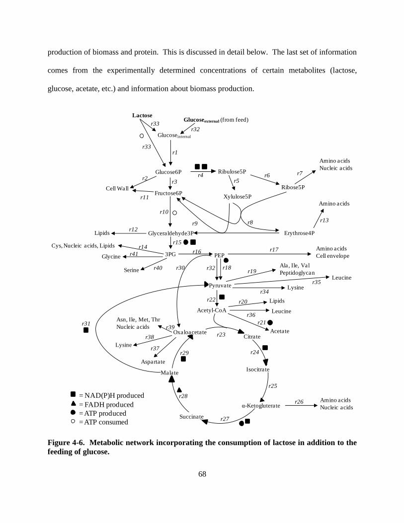
68
production of biomass and protein. This is discussed in detail below. The last set of information
comes from the experimentally determined concentrations of certain metabolites (lactose,
glucose, acetate, etc.) and information about biomass production.
Figure 4-6. Metabolic network incorporating the consumption of lactose in addition to the
feeding of glucose.
Amino acids
Cell envelope
Cys, Nucleic acids, Lipids
Ribulose5P
Amino acids
Nucleic acids
Cell Wall
Lipids
Glucoseinternal
Glucose6P
Fructose6P
Glyceraldehyde3P
3PG PEP
Ribose5P
Xylulose5P
Erythrose4P
Amino acids
Ala, Ile, Val
Peptidoglycan
Citrate
α-Ketogluterate
Oxaloacetate
Amino acids
Nucleic acids
Lipids
Acetate
Pyruvate
Acetyl-CoA
r1
r18
r2r3
r4
r10
r5r6 r7
r13r9
r12
r15
r11
r16r14 r17
r19r32
r22 r20
r23
r24
r25
r27
r26
r21
Lactose
r8
Isocitrate
r29
r28
Glucoseexternal (from feed)r33
r32
r30
Asn, Ile, Met, Thr
Nucleic acids
r34Lysine
Leucine
Glycine
r40
r35
Serine
r39
Leuciner36
Lysine
r38
Aspartate
r37
Succinate
Malate
r33
r31
r41
= NAD(P)H produced
= FADH produced
= ATP produced
= ATP consumed
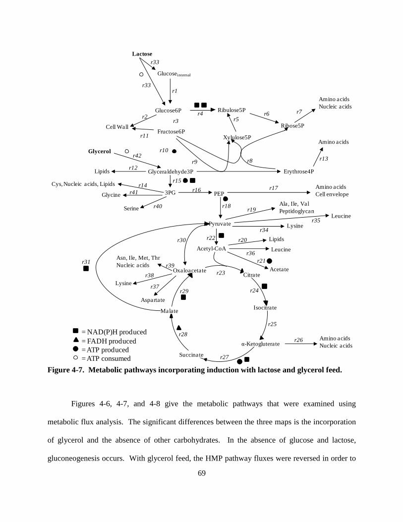
69
Figure 4-7. Metabolic pathways incorporating induction with lactose and glycerol feed.
Figures 4-6, 4-7, and 4-8 give the metabolic pathways that were examined using
metabolic flux analysis. The significant differences between the three maps is the incorporation
of glycerol and the absence of other carbohydrates. In the absence of glucose and lactose,
gluconeogenesis occurs. With glycerol feed, the HMP pathway fluxes were reversed in order to
Amino acids
Cell envelope
Cys, Nucleic acids, Lipids
Ribulose5P
Amino acids
Nucleic acids
Cell Wall
Lipids
Glucoseinternal
Glucose6P
Fructose6P
Glyceraldehyde3P
3PG PEP
Ribose5P
Xylulose5P
Erythrose4P
Amino acids
Ala, Ile, Val
Peptidoglycan
Citrate
α-Ketogluterate
Oxaloacetate
Amino acids
Nucleic acids
Lipids
Acetate
Pyruvate
Acetyl-CoA
r1
r18
r2r3
r4
r10
r5r6 r7
r13r9
r12
r15
r11
r16r14 r17
r19
r22 r20
r23
r24
r25
r27
r26
r21
Lactose
r8
Isocitrate
r29
r28
r33
r30
Asn, Ile, Met, Thr
Nucleic acids
r34Lysine
Leucine
Glycine
r40
r35
Serine
r39
Leuciner36
Lysine
r38
Aspartate
r37
Succinate
Malate
r33
r31
r41
Glycerolr42
= NAD(P)H produced
= FADH produced
= ATP produced
= ATP consumed
70
make glucose from glycerol. It is also important to reverse these fluxes so that the necessary
precursors can be synthesized from other HMP pathway components (e.g. amino acids and
nucleic acids from ribose 5-phosphate). Upon glycerol uptake, an ATP molecule is required for
the phosphorylation of glycerol and ultimate synthesis of glyceraldehyde 3-phosphate. The map
in Figure 4-7 was used when lactose was still present in the system and glycerol was used as the
feed source. Figure 4-8 is representative of the fluxes when lactose was no longer present in the
media and glycerol was used as a feed source. With this system, there are two possible
scenarios. One involves simply removing the internal glucose flux and lactose flux from the map
in Figure 4-7. The other possibility is that the carbon from the glycerol flux is stored as
glycogen. An additional ATP molecule is required for this step. The pathway representing this
phenomenon is indicated by the dashed oval in Figure 4-8.

71
Figure 4-8. Flux pathway when glycerol is the only carbohydrate fed into the system and
present in the media (after lactose has been depleted).
The corresponding chemical reactions are given in the Appendix (9.5), but the
mathematical representation of these reactions is given below.
Amino acids
Cell envelope
Cys, Nucleic acids, Lipids
Ribulose5P
Amino acids
Nucleic acids
Cell Wall
Lipids
Glucoseinternal
Glucose6P
Fructose6P
Glyceraldehyde3P
3PG PEP
Ribose5P
Xylulose5P
Erythrose4P
Amino acids
Ala, Ile, Val
Peptidoglycan
Citrate
α-Ketogluterate
Oxaloacetate
Amino acids
Nucleic acids
Lipids
Acetate
Pyruvate
Acetyl-CoA
r1
r18
r2r3
r4
r10
r5r6 r7
r13r9
r12
r15
r11
r16r14 r17
r19
r22 r20
r23
r24
r25
r27
r26
r21
r8
Isocitrate
r29
r28
r30
Asn, Ile, Met, Thr
Nucleic acids
r34Lysine
Leucine
Glycine
r40
r35
Serine
r39
Leuciner36
Lysine
r38
Aspartate
r37
Succinate
Malate
r31
r41
Glycerolr42
= NAD(P)H produced
= FADH produced
= ATP produced
= ATP consumed
Glycogenr43

72
Intermediates:
x1 = r32 + r33 – r1 Balance on internal glucose
x2 = r1+ r33 – r2 – r3 – r4 Balance on glucose 6-phosphate
x3 = r4 – r5 – r6 Balance on ribulose 5-phosphate
x4 = r6 – r7 – r8 Balance on ribose 5-phosphate
x5 = r5 – r8 – r9 Balance on xylulose 5-phosphate
x6 = r3 + r8 + r9 – r10 – r11 Balance on fructose 6-phosphate
x7 = r8 – r9 – r13 Balance on erythrose 4-phosphate
x8 = 2* r10 + r9 + r42 – r12 – r15 Balance on glyceraldehyde 3P
x9 = r15 – r16 – r14 – r40 – r41 Balance on 3-phosphoglycerate
x10 = r16 – r17 – r18 – r30 – r32 Balance on phosphoenol pyruvate
x11 = r31 + r32 + r18 – r19– r22 – r34 – r35 Balance on pyruvate
x12 = r22 – r20 – r21 – r23 – r36 Balance on acetyl-CoA
x13 = r23 – r24 Balance on citrate
x14 = r24 – r25 Balance on isocitrate
x15 = r25 – r26 – r27 Balance on α-ketoglutarate
x16 = r27 – r28 Balance on succinate
x17 = r28 – r29 – r31 Balance on malate
x18 = r29 + r30 – r23 – r37 – r38 – r39 Balance on oxaloacetate
Precursors:
x19 = r7 = ρ7*D AA, NA from ribose 5-phosphate
x20 = r13 = ρ13*D AA from erythrose 4-phosphate
x21 = r17 = ρ17*D AA, Cell envelope from PEP
x22 = r19 = ρ19*D AA, peptidoglycan from pyruvate
x23 = r20 = ρ20*D AA, Lipids from AcCoA
x24 = r26 = ρ26*D AA, NA from α-ketoglutarate
x25 = r39 = ρ39*D AA, NA from oxaloacetate
x26 = r14 = ρ14*D AA, NA, Lipids from 3PG
x27 = r12 = ρ12*D Lipids from glyceraldehyde 3P
x28 = r11 = ρ11*D Cell wall from fructose 6-phosphate
x29 = r2 = ρ2*D Cell wall from glucose 6-phosphate
x30 = r34 = ρLys_PYR*D Lysine from pyruvate
x31 = r35 = ρLeu_PYR*D Leucine from pyruvate
x32 = r37 = ρAsp_OA*D Asparate from OA
x33 = r38 = ρLys_OA*D Lysine from OA
x34 = r36 = ρLeu_AcCoa*D Leucine from acetyl-CoA
x35 = r40 = ρSer_3PG*D Serine from 3-phosphoglycerate
x36 = r41 = ρGly_3PG*D Glycine from 3-phosphoglycerate
x40 = 2*r4 + r24 = 18*D NADPH balance
Measureable components:
x37 = r21 = Cacetate*(D/X) Balance on acetate
x38 = r32 = Cglucose*(D/X) External glucose uptake
x39 = 2*r33 = Clactose*(D/X) Lactose uptake (breakdown)
x41 = r42 = Cglycerol*(D/X) Balance on glycerol

73
For the intermediates given above, xi = 0 due to the pseudo-steady state assumption (no
accumulation of metabolic intermediates). In order to calculate the precursor pool demands for
cell maintenance along with production of target protein, one must have information about the
requirements for cell growth. This information, along with the metabolic precursors from which
the amino acids, dNTP's, etc. are derived, was compiled and is given in Table 4-3. The
information about the type and amount of precursor required for the target protein is given in
Table 4-4. This information was calculated from the amino acid composition (Table 4-1).
Assuming that P is the mass percentage of target protein production to total cell mass, the
calculation of precursor demand (given by ρ) can be written as the following:
ρ = P*ρP + (1-P)*ρc_p + ρc_o (4.13)
In this equation, ρP represents the precursor demand from target protein expression (sum of the
demands for the target protein amino acids); ρc_p represents the precursor demand from proteins
for cellular composition (sum of the demands for amino acids); and ρc_o represents the precursor
demand for other cellular components (non-protein sum). As an example, consider that the
percentage of target protein is 10 and examine the requirements for 3-phosphoglycerate (3PG).
Then, the precursor demand is:
ρ = P*ρP + (1-P)*ρc_p + ρc_o = 0.1*1.275 + 0.9*0.874 + 0.6164 = 1.5305 (4.14)
The values for ρi are given in Tables 4-3 and 4-4 for each metabolic precursor. These
calculations were performed for all of the metabolic precursors and are shown in Section 9.6.
The precursor values were multiplied by the dilution rate (growth rate - D) to get the final
amounts needed for protein expression and cell growth. This information was contained in the

74
accumulation vector because these minimal amounts of metabolites are required for cell
maintenance and protein expression.
Unlike other metabolic flux models, information about the addition of the amino acids in
the media was contained in this model. As shown in Figures 4-6 and 4-7, pyruvate, acetyl-CoA,
3-phosphoglycerate, and oxaloacetate are all metabolic precursors for certain amino acids that
were contained in the media. Thus, these precursors were not in as high demand for production
of certain amino acids. This information was included by considering the fluxes of these amino
acids (Lys, Leu, Asp, Gly, Ser) separate from the total amino acid flux. Then, since the
concentration of the amino acid was known, this information was added in the x vector.
Consider, for example, the flux of leucine from acetyl-CoA. The individual precursor demand
for leucine was subtracted from the total precursor demand because the demand was not as high
due to the presence of leucine in the media. The same logic followed for the other amino acids
in the media. Since leucine and lysine are produced from two different metabolic precursors,
these amino acids appear two times as a component in the system (each component from their
different metabolic precursors).
Additionally, since the final amount of product was known, the amount of each amino
acid (Ci) required for production was calculated by multiplying the amount required per gram
protein (Ci_protein, Table 4-4) and adding this to the product of the amount required for cell
maintenance (Ci_cell, Table 4-3) and grams of biomass:
Ci = Ci_cell*Biomass + Ci_protein*Proteintotal (4.15)
The information about carbohydrates and biomass also helped constrain the system.
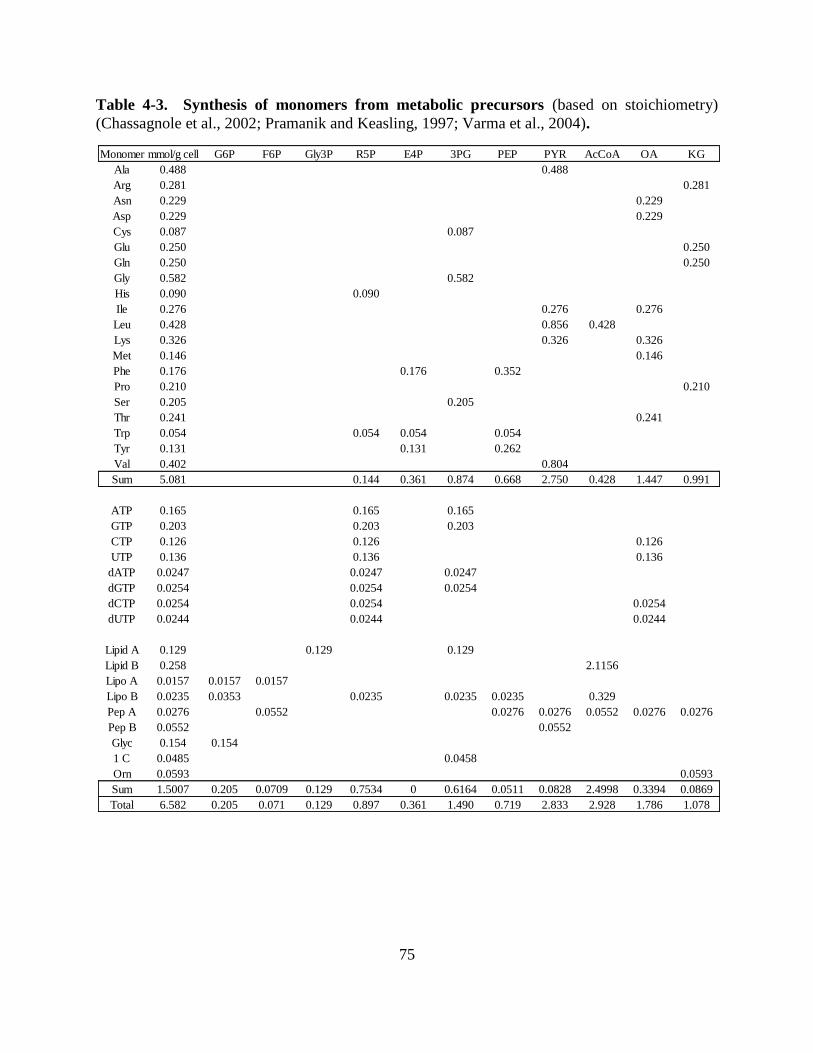
75
Table 4-3. Synthesis of monomers from metabolic precursors (based on stoichiometry)
(Chassagnole et al., 2002; Pramanik and Keasling, 1997; Varma et al., 2004).
Monomer mmol/g cell G6P F6P Gly3P R5P E4P 3PG PEP PYR AcCoA OA KG
Ala 0.488 0.488
Arg 0.281 0.281
Asn 0.229 0.229
Asp 0.229 0.229
Cys 0.087 0.087
Glu 0.250 0.250
Gln 0.250 0.250
Gly 0.582 0.582
His 0.090 0.090
Ile 0.276 0.276 0.276
Leu 0.428 0.856 0.428
Lys 0.326 0.326 0.326
Met 0.146 0.146
Phe 0.176 0.176 0.352
Pro 0.210 0.210
Ser 0.205 0.205
Thr 0.241 0.241
Trp 0.054 0.054 0.054 0.054
Tyr 0.131 0.131 0.262
Val 0.402 0.804
Sum 5.081 0.144 0.361 0.874 0.668 2.750 0.428 1.447 0.991
ATP 0.165 0.165 0.165
GTP 0.203 0.203 0.203
CTP 0.126 0.126 0.126
UTP 0.136 0.136 0.136
dATP 0.0247 0.0247 0.0247
dGTP 0.0254 0.0254 0.0254
dCTP 0.0254 0.0254 0.0254
dUTP 0.0244 0.0244 0.0244
Lipid A 0.129 0.129 0.129
Lipid B 0.258 2.1156
Lipo A 0.0157 0.0157 0.0157
Lipo B 0.0235 0.0353 0.0235 0.0235 0.0235 0.329
Pep A 0.0276 0.0552 0.0276 0.0276 0.0552 0.0276 0.0276
Pep B 0.0552 0.0552
Glyc 0.154 0.154
1 C 0.0485 0.0458
Orn 0.0593 0.0593
Sum 1.5007 0.205 0.0709 0.129 0.7534 0 0.6164 0.0511 0.0828 2.4998 0.3394 0.0869
Total 6.582 0.205 0.071 0.129 0.897 0.361 1.490 0.719 2.833 2.928 1.786 1.078
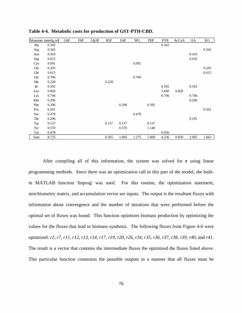
76
Table 4-4. Metabolic costs for production of GST-PTH-CBD.
After compiling all of this information, the system was solved for r using linear
programming methods. Since there was an optimization call in this part of the model, the built-
in MATLAB function 'linprog' was used. For this routine, the optimization statement,
stoichiometric matrix, and accumulation vector are inputs. The output is the resultant fluxes with
information about convergence and the number of iterations that were performed before the
optimal set of fluxes was found. This function optimizes biomass production by optimizing the
values for the fluxes that lead to biomass synthesis. The following fluxes from Figure 4-6 were
optimized: r2, r7, r11, r12, r13, r14, r17, r19, r20, r26, r34, r35, r36, r37, r38, r39, r40, and r41.
The result is a vector that contains the intermediate fluxes the optimized the fluxes listed above.
This particular function constrains the possible outputs in a manner that all fluxes must be
Monomer mmol/g cell G6P F6P Gly3P R5P E4P 3PG PEP PYR AcCoA OA KG
Ala 0.342 0.342
Arg 0.342 0.342
Asn 0.410 0.410
Asp 0.615 0.610
Cys 0.091 0.091
Glu 0.205 0.205
Gln 0.615 0.615
Gly 0.706 0.706
His 0.228 0.228
Ile 0.592 0.592 0.592
Leu 0.820 1.640 0.820
Lys 0.706 0.706 0.706
Met 0.296 0.296
Phe 0.296 0.296 0.592
Pro 0.501 0.501
Ser 0.478 0.478
Thr 0.296 0.291
Trp 0.137 0.137 0.137 0.137
Tyr 0.570 0.570 1.140
Val 0.478 0.956
Sum 8.725 0.365 1.003 1.275 1.869 4.236 0.820 2.905 1.663

77
greater than or equal to zero. This aided in reducing the solution space for the minimization
routine.
The resultant fluxes for this model gave a final snapshot of the system with regard to
concentrations and production of biomass components. Only the final concentrations for acetate,
glucose, lactose, glycerol, and biomass were used in the calculations that helped determine the
fluxes. For many of the experiments, modeling the system using only the final concentrations
for carbohydrates and biomass was not sufficient to describe the system as a whole due to the
early elapsed time in which the stationary phase of the fermentation system was reached. In this
case, it was interesting to examine the change in the fluxes from time point to time point by
using the experimental data taken from the experiment. Once again, by optimizing the fluxes
from metabolic precursors to cell wall components, the overall biomass formation was
optimized. The same fluxes were optimized as those in the overall snapshot model (described in
the previous paragraph). These fluxes contribute to the formation of amino acids, cell wall,
lipids, nucleic acids, cell envelope, and peptidoglycan. The precursors that are required for cell
formation and protein production were calculated the same way as before.
After performing the optimization routine, the output was the resultant fluxes that
allowed for optimization of the biomass. Here, A was the same stoichiometric matrix as before
and x contained information about the intermediates (concentration is zero), the precursor
information, and concentrations determined from the experiments. However, unlike before, the
accumulation vector contained information about the fluxes of carbons at each time step were
used. For example, samples were taken at 16, 18, 20, and 22 hours for the 12 hr lactose-induced
experiment. The concentration changes of lactose and glucose (or glycerol) between each time

78
point were calculated on a mM/hr basis. The biomass was also averaged and the acetate
production was calculated. For this step-by-step analysis, the dilution factor was not required for
calculation of the concentrations due to the averaging of the concentrations over the time interval
at which the samples were taken (one or two hours depending on the experiment).
As a test to the validity of the model, the next experimental concentration can be
compared with the simulated concentration by using the flux information and methods
comparable to Euler's method:
Ci+1 = Ci + ri*Δt*Biomass (4.16)
Here, multiplying the flux for glucose or glycerol, acetate, or lactose from the simulation by the
time step and the averaged biomass (2 hours in most cases) and adding this product to the initial
concentration yielded information about the new concentration. The MATLAB code for the
generation of the metabolic flux analysis is given in the Appendix (Section 9.8).
After solving for the fluxes, the ATP balance was used to calculate the yield of cells from
ATP. This provided useful information about the effect that different inducers and feed sources
have on the biomass production from ATP. The balance equation for ATP depended on the
fermentation experiment that was modeled. For example, the breakdown of lactose to glucose 6-
phosphate through galactose metabolism requires a molecule of ATP. Similarly, glycogen
synthesis and the synthesis of glyceraldehyde 3-phosphate from glycerol both require ATP.
However, the contribution of NAD(P)H and FADH to ATP synthesis did not depend on the
experimental method. For each experiment, the following balances exist:
NAD(P)H = 2*r4 + r15 + r22 + r24 + r27 + r29 + r31 (4.17)
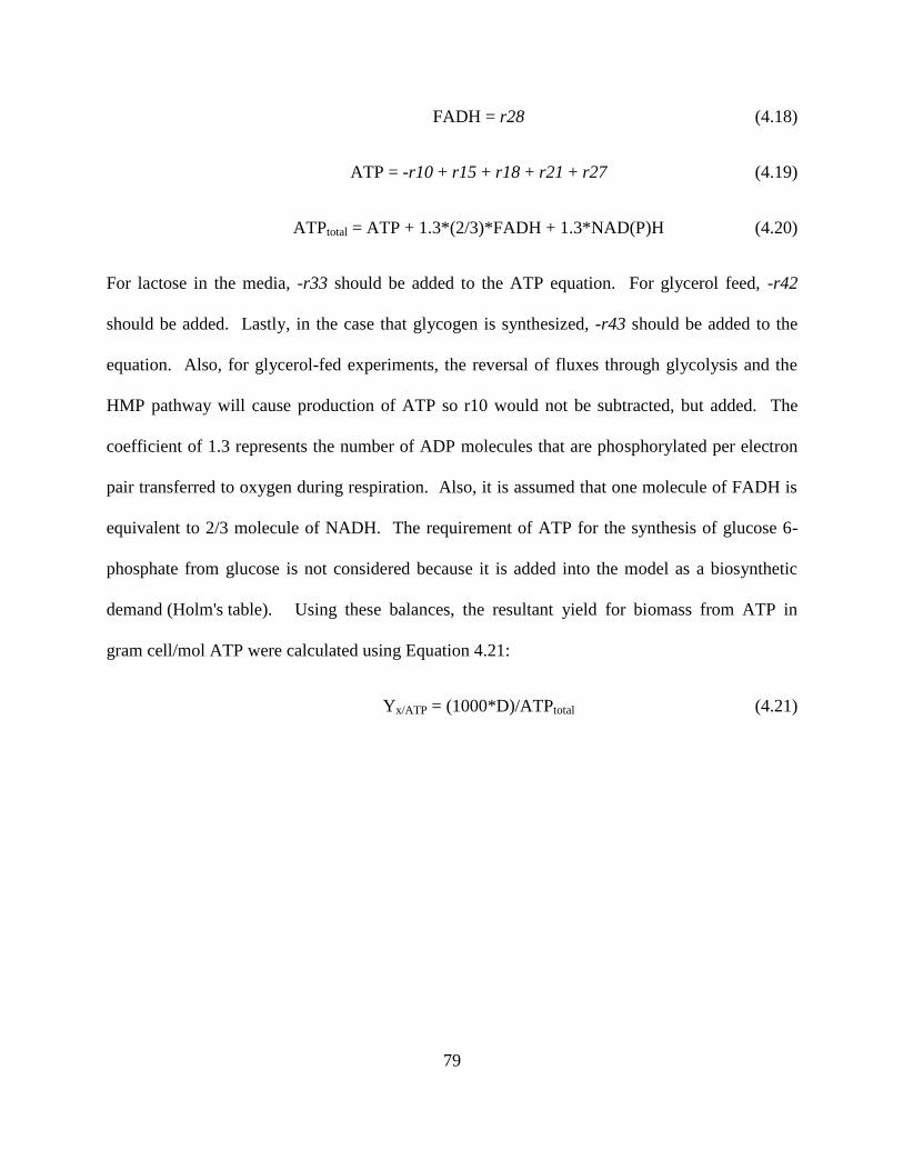
79
FADH = r28 (4.18)
ATP = -r10 + r15 + r18 + r21 + r27 (4.19)
ATPtotal = ATP + 1.3*(2/3)*FADH + 1.3*NAD(P)H (4.20)
For lactose in the media, -r33 should be added to the ATP equation. For glycerol feed, -r42
should be added. Lastly, in the case that glycogen is synthesized, -r43 should be added to the
equation. Also, for glycerol-fed experiments, the reversal of fluxes through glycolysis and the
HMP pathway will cause production of ATP so r10 would not be subtracted, but added. The
coefficient of 1.3 represents the number of ADP molecules that are phosphorylated per electron
pair transferred to oxygen during respiration. Also, it is assumed that one molecule of FADH is
equivalent to 2/3 molecule of NADH. The requirement of ATP for the synthesis of glucose 6-
phosphate from glucose is not considered because it is added into the model as a biosynthetic
demand (Holm's table). Using these balances, the resultant yield for biomass from ATP in
gram cell/mol ATP were calculated using Equation 4.21:
Yx/ATP = (1000*D)/ATPtotal (4.21)

80
5. Results and discussion
5.1 Shake flask cultivations
A number of experiments were performed to examine the effects of media on the growth
of E. coli harboring plasmid pCHC305. From this point on, the bacterial strain will simply be
referred to as pCHC305 and target therapeutic protein will be referred to as GST-PTH-CBD.
Figure 5-1 shows results from the study of growth on LB and its dependency on glucose. As
shown in Figure 5-1, LB supplemented with glucose allowed for slightly higher optical densities.
Though, this increase was not significant, as the growth rate for both cultures was equivalent.
However, LB supplemented with glucose did not enhance therapeutic protein production as
evident by similar band intensities of protein near the target molecular weight in Figure 5-2.
Equal concentrations of total protein were loaded to each lane in the SDS-PAGE gel. GST-PTH-
CBD runs at approximately 44 kDa on a 12.5% gel. It is interesting to note that the length of the
induction period also did not have an effect on protein production when cells were grown in LB
or LB supplemented with glucose and induced with IPTG. This indicated that there was a basal
expression level of target protein in the absence of inducer.
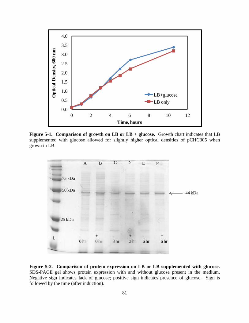
81
Figure 5-1. Comparison of growth on LB or LB + glucose. Growth chart indicates that LB
supplemented with glucose allowed for slightly higher optical densities of pCHC305 when
grown in LB.
Figure 5-2. Comparison of protein expression on LB or LB supplemented with glucose. SDS-PAGE gel shows protein expression with and without glucose present in the medium.
Negative sign indicates lack of glucose; positive sign indicates presence of glucose. Sign is
followed by the time (after induction).
0.0
0.5
1.0
1.5
2.0
2.5
3.0
3.5
4.0
0 2 4 6 8 10 12
Op
tica
l D
ensi
ty,
60
0 n
m
Time, hours
LB+glucose
LB only
75 kDa
50 kDa
25 kDa
A B C D E F
-
0 hr
+
0 hr
-
3 hr
+
3 hr
-
6 hr
+
6 hrL
44 kDa

82
While growth curves are important to consider when choosing a proper medium, protein
expression on the medium is perhaps more important. The next step was to test the expression of
GST-PTH-CBD when using a defined medium, such as M9 supplemented with glucose. To
examine the expression of GST-PTH-CBD on M9 supplemented with glucose, lysates from cells
grown on M9 + 10 g/l glucose or LB were loaded to a 12.5% SDS-PAGE gel. The same
concentration of protein was loaded to each lane in order for direct comparison of target protein
production. As indicated by the intensity of the band in lane 4 at 44 kDa in Figure 5-3, M9 +
glucose allowed for higher expression of GST-PTH-CBD (compared to lysates from cells grown
on LB). For the remainder of this dissertation, M9 + glucose will refer to M9 supplemented with
10 g/l of glucose.
Figure 5-3. Comparison of GST-PTH-CBD expression from cells grown on LB or M9. Lane 1 – molecular weight standard; 2 – pre-induction, M9 + glucose; 3 – pre-induction, LB; 4 –
post induction, M9 + glucose; 5 – post induction, LB.
1 2 3 4 5
50 kDa
37 kDa
25 kDa44 kDa
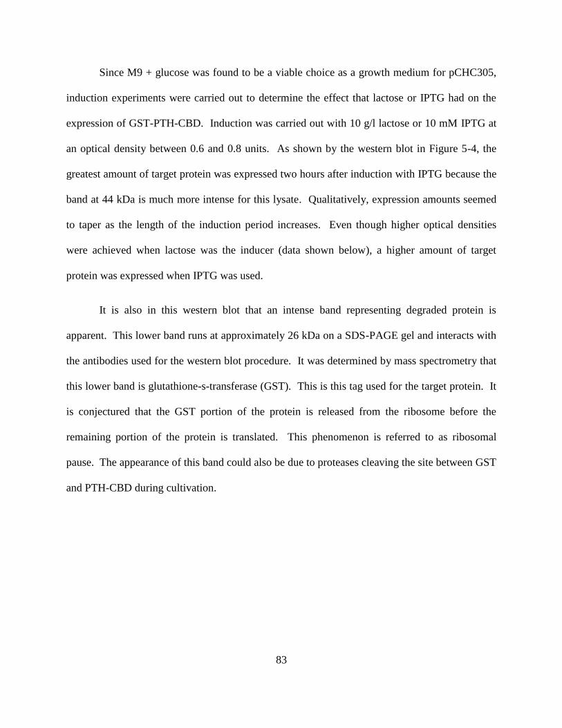
83
Since M9 + glucose was found to be a viable choice as a growth medium for pCHC305,
induction experiments were carried out to determine the effect that lactose or IPTG had on the
expression of GST-PTH-CBD. Induction was carried out with 10 g/l lactose or 10 mM IPTG at
an optical density between 0.6 and 0.8 units. As shown by the western blot in Figure 5-4, the
greatest amount of target protein was expressed two hours after induction with IPTG because the
band at 44 kDa is much more intense for this lysate. Qualitatively, expression amounts seemed
to taper as the length of the induction period increases. Even though higher optical densities
were achieved when lactose was the inducer (data shown below), a higher amount of target
protein was expressed when IPTG was used.
It is also in this western blot that an intense band representing degraded protein is
apparent. This lower band runs at approximately 26 kDa on a SDS-PAGE gel and interacts with
the antibodies used for the western blot procedure. It was determined by mass spectrometry that
this lower band is glutathione-s-transferase (GST). This is this tag used for the target protein. It
is conjectured that the GST portion of the protein is released from the ribosome before the
remaining portion of the protein is translated. This phenomenon is referred to as ribosomal
pause. The appearance of this band could also be due to proteases cleaving the site between GST
and PTH-CBD during cultivation.

84
Figure 5-4. Western blot of lysates from lactose or IPTG induction with M9 + glucose
media. Lane 1 – molecular weight standard; 2 – pre-induction, IPTG; 3 – pre-induction, lactose;
4 – 2 hr post IPTG; 5 – 2 hr post lactose; 6 – 4 hr post IPTG; 7 – 4 hr post lactose; 8 – final,
IPTG; 9 – final, lactose. Basal amount of target protein is present prior to induction.
To further increase therapeutic protein expression, M9 + glucose was supplemented with
amino acids. Growth on M9 + glucose supplemented with amino acids and thiamine was also
investigated. As shown in Figure 5-5, using M9 + glucose or M9 + glucose supplemented with
amino acids (with or without thiamine) extended the time at which the culture reached the
stationary phase of growth. Additionally, cultures grown on M9 + glucose supplemented with
amino acids achieved higher optical densities than those grown on M9 + glucose without amino
acids.
1 2 3 4 5 6 7 8 9
50
37 44 kDa, GST-PTH-CBD
26 kDa, GST
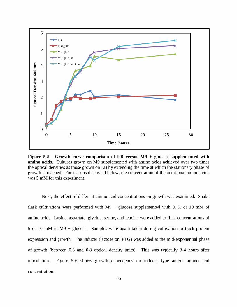
85
Figure 5-5. Growth curve comparison of LB versus M9 + glucose supplemented with
amino acids. Cultures grown on M9 supplemented with amino acids achieved over two times
the optical densities as those grown on LB by extending the time at which the stationary phase of
growth is reached. For reasons discussed below, the concentration of the additional amino acids
was 5 mM for this experiment.
Next, the effect of different amino acid concentrations on growth was examined. Shake
flask cultivations were performed with M9 + glucose supplemented with 0, 5, or 10 mM of
amino acids. Lysine, aspartate, glycine, serine, and leucine were added to final concentrations of
5 or 10 mM in M9 + glucose. Samples were again taken during cultivation to track protein
expression and growth. The inducer (lactose or IPTG) was added at the mid-exponential phase
of growth (between 0.6 and 0.8 optical density units). This was typically 3-4 hours after
inoculation. Figure 5-6 shows growth dependency on inducer type and/or amino acid
concentration.
0
1
2
3
4
5
6
0 5 10 15 20 25 30
Op
tica
l D
ensi
ty, 600 n
m
Time, hours
LB
LB+gluc
M9+gluc
M9+gluc+aa
M9+gluc+aa+thia

86
(a)
(b)
Figure 5-6. Growth characteristics of induced cultures grown on M9 supplemented with
different concentrations of amino acids. (a) Cultures were induced with lactose. Shake flasks
supplemented with amino acids reached higher optical densities than that without the addition.
(b) Cultures were induced with IPTG. In both figures, M9 was supplemented with 10 g/l
glucose.
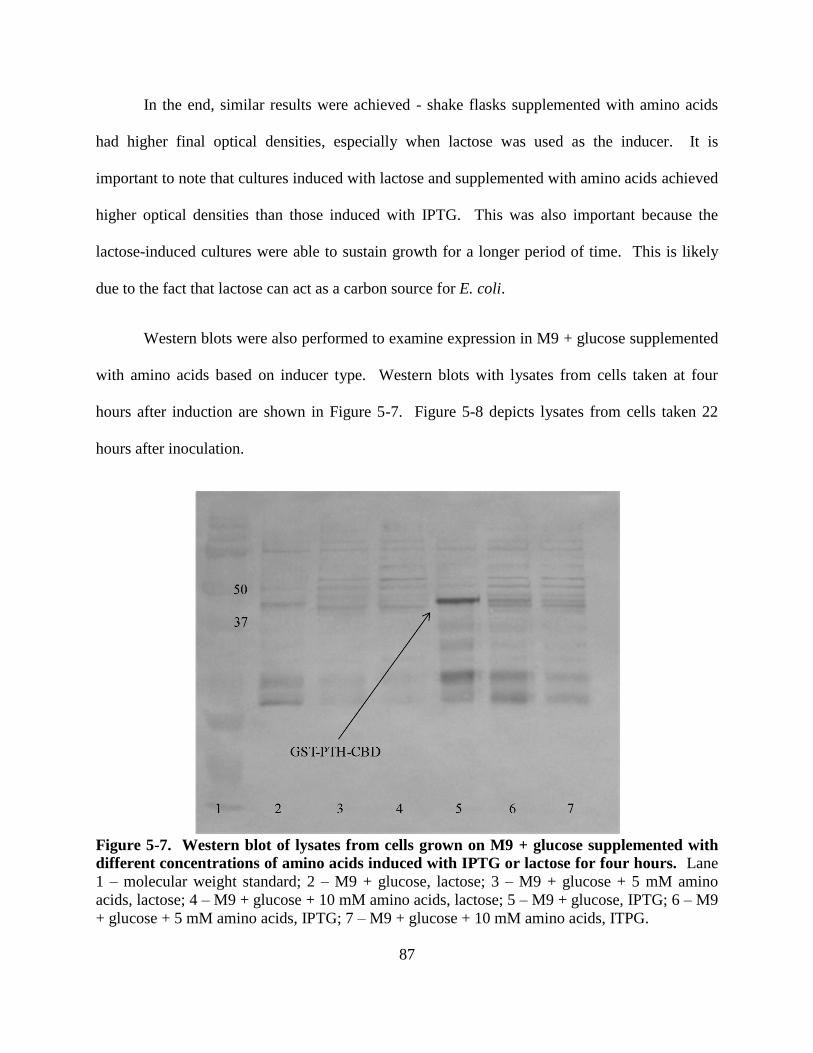
87
In the end, similar results were achieved - shake flasks supplemented with amino acids
had higher final optical densities, especially when lactose was used as the inducer. It is
important to note that cultures induced with lactose and supplemented with amino acids achieved
higher optical densities than those induced with IPTG. This was also important because the
lactose-induced cultures were able to sustain growth for a longer period of time. This is likely
due to the fact that lactose can act as a carbon source for E. coli.
Western blots were also performed to examine expression in M9 + glucose supplemented
with amino acids based on inducer type. Western blots with lysates from cells taken at four
hours after induction are shown in Figure 5-7. Figure 5-8 depicts lysates from cells taken 22
hours after inoculation.
Figure 5-7. Western blot of lysates from cells grown on M9 + glucose supplemented with
different concentrations of amino acids induced with IPTG or lactose for four hours. Lane
1 – molecular weight standard; 2 – M9 + glucose, lactose; 3 – M9 + glucose + 5 mM amino
acids, lactose; 4 – M9 + glucose + 10 mM amino acids, lactose; 5 – M9 + glucose, IPTG; 6 – M9
+ glucose + 5 mM amino acids, IPTG; 7 – M9 + glucose + 10 mM amino acids, ITPG.
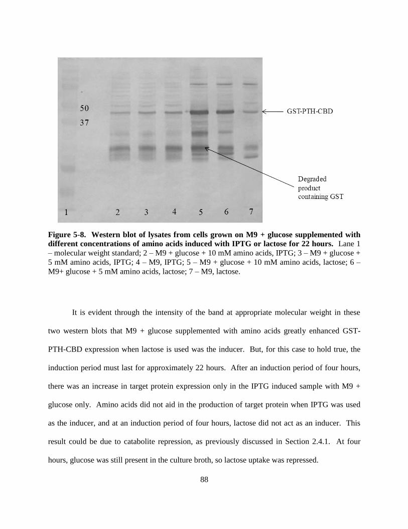
88
Figure 5-8. Western blot of lysates from cells grown on M9 + glucose supplemented with
different concentrations of amino acids induced with IPTG or lactose for 22 hours. Lane 1
– molecular weight standard; 2 – M9 + glucose + 10 mM amino acids, IPTG; 3 – M9 + glucose +
5 mM amino acids, IPTG; 4 – M9, IPTG; 5 – M9 + glucose + 10 mM amino acids, lactose; 6 –
M9+ glucose + 5 mM amino acids, lactose; 7 – M9, lactose.
It is evident through the intensity of the band at appropriate molecular weight in these
two western blots that M9 + glucose supplemented with amino acids greatly enhanced GST-
PTH-CBD expression when lactose is used was the inducer. But, for this case to hold true, the
induction period must last for approximately 22 hours. After an induction period of four hours,
there was an increase in target protein expression only in the IPTG induced sample with M9 +
glucose only. Amino acids did not aid in the production of target protein when IPTG was used
as the inducer, and at an induction period of four hours, lactose did not act as an inducer. This
result could be due to catabolite repression, as previously discussed in Section 2.4.1. At four
hours, glucose was still present in the culture broth, so lactose uptake was repressed.

89
As shown in Figure 5-8, pCHC305 grown on M9 supplemented with 10 mM amino acids
and induced with lactose expressed the greatest amount of GST-PTH-CBD. This sample also
had the highest concentration of degraded product, as the intensity of lower bands in lane 5 was
greater. Additionally, the amount of sodium hydroxide that was needed to increase the pH of the
medium supplemented with 10 mM amino acids to 6.8 caused some of the salts to precipitate. It
is for these reasons that it was decided to use a 5 mM amino acid concentration to supplement
M9 in further experiments.
Since amino acids appear to aid in protein expression when lactose is used as an inducer,
experiments were performed to see if auto-induction would work for shake flasks. This could
automate the induction process, as everything is in the medium prior to cultivation. Shake flask
experiments were carried out to monitor the difference between auto-induction and manual
induction. Unlike work done by others, there were no undefined components added to the
medium, for the auto-induction experiment. M9 + glucose was used, with the only addition
being lactose and amino acids. After analysis of the samples taken from shake flasks, it was
determined that auto-induction did not have an effect on protein expression. The samples with
lactose initially present and lactose manually added at the mid-exponential phase did not exhibit
any significant increases. This finding makes sense with the analysis of carbohydrate
concentrations portrayed in Figure 5-9. HPLC results indicated that the lactose concentration did
not change throughout the cultivation, and after 25 hours, there was still glucose present in the
medium. Although, as shown in Figures 5-7 and 5-8, induction via lactose must have occurred
between 4 and 22 hours after induction. At some point when the glucose concentrations
decreased, catabolite repression decreased to allow induction with lactose.
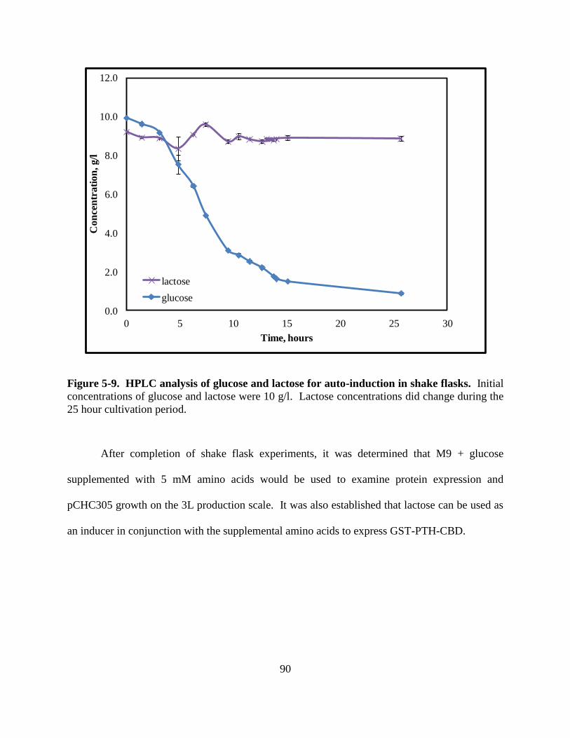
90
Figure 5-9. HPLC analysis of glucose and lactose for auto-induction in shake flasks. Initial
concentrations of glucose and lactose were 10 g/l. Lactose concentrations did change during the
25 hour cultivation period.
After completion of shake flask experiments, it was determined that M9 + glucose
supplemented with 5 mM amino acids would be used to examine protein expression and
pCHC305 growth on the 3L production scale. It was also established that lactose can be used as
an inducer in conjunction with the supplemental amino acids to express GST-PTH-CBD.
0.0
2.0
4.0
6.0
8.0
10.0
12.0
0 5 10 15 20 25 30
Con
cen
trati
on
, g/l
Time, hours
lactose
glucose
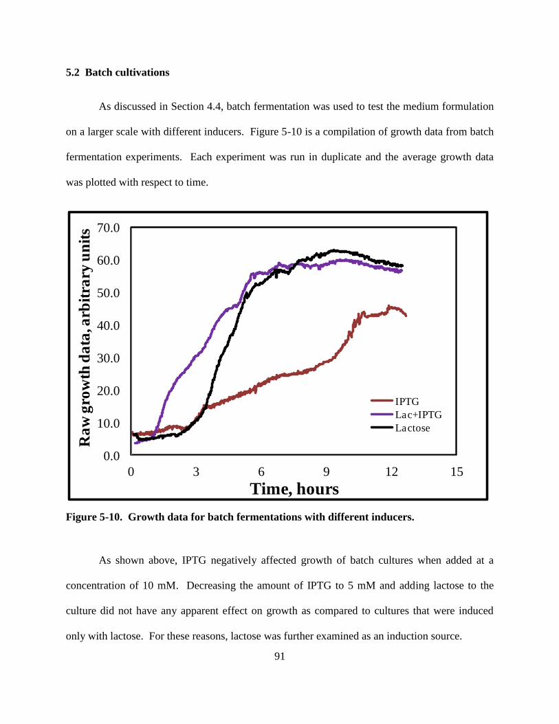
91
5.2 Batch cultivations
As discussed in Section 4.4, batch fermentation was used to test the medium formulation
on a larger scale with different inducers. Figure 5-10 is a compilation of growth data from batch
fermentation experiments. Each experiment was run in duplicate and the average growth data
was plotted with respect to time.
Figure 5-10. Growth data for batch fermentations with different inducers.
As shown above, IPTG negatively affected growth of batch cultures when added at a
concentration of 10 mM. Decreasing the amount of IPTG to 5 mM and adding lactose to the
culture did not have any apparent effect on growth as compared to cultures that were induced
only with lactose. For these reasons, lactose was further examined as an induction source.
0.0
10.0
20.0
30.0
40.0
50.0
60.0
70.0
0 3 6 9 12 15
Ra
w g
row
th d
ata
, arb
itra
ry u
nit
s
Time, hours
IPTG
Lac+IPTG
Lactose
92
5.3 Fed-batch cultivations
As discussed in Section 2.3, fed-batch fermentation is used to achieve high cell density
cultivations. For this work, an exponential feeding strategy was employed. This strategy and
feeding profile development was thoroughly discussed in Section 4.5. To calculate product per
gram cell basis (product yield), the concentration in terms of mg/l (found by densitometry) was
divided by the value for the dry cell weight per liter (as determined by moisture analyzer). The
value of mg/g DCW takes into account the denseness of the culture to give target protein
concentration on a per gram cell basis. When reporting data for fermentation experiments, dry
weight is often used because it accounts for difference in moisture content. For downstream
processing (centrifugation, purification, etc.), the amount of product per cell is important to
consider because of the amount of cells that must be processed. This type of calculation can also
relate production of target protein to its volumetric productivity. For example, the goal for
recombinant fed-batch fermentation is to produce a large number of cells. However, if a low
number of cells is produced, but the target protein per cell is high, then the volumetric
productivity is high. While this information is useful, it is also important to consider the total
amount of product produced for a given experiment.
In many industrial applications, it may be desired to produce a certain amount of product.
In this case, it is not as important to consider the amount of cells required to produce this product
because this cost is ultimately passed down to the end-user. Needless to say, the results for
protein expression are given in both units.

93
5.3.1 Cultures fed with glucose as major carbon source
5.3.1.1 Lactose induction after inoculation
The first fed-batch experiment utilized a feeding profile that exponentially delivered feed
at rates between 0.1 and 0.3 ml/min. The growth rate for the profile was set at 0.2 hr-1
, which is
within range of suggested growth rates for exponentially feeding E. coli cultures. This method is
henceforth referred to as the saw-tooth method because of its characteristic feed profile. The
cultivation was completely glucose limited, as glucose assays indicated that there was no glucose
left in the culture broth. It was also induced with lactose 11 hours after inoculation. Figure 5-11
represents the growth curve for this type of cultivation. The final dry cell weight for this
fermentation type was 50 grams. The average total dry cell weight of two runs is plotted versus
time.
Figure 5-11. Growth curve for saw-tooth feeding method with induction at 11 hours with
lactose. The arrow indicates when induction occurred.
0
10
20
30
40
50
60
70
80
0 5 10 15 20 25 30
dry
cel
l w
eig
ht,
gra
ms
Time, hours
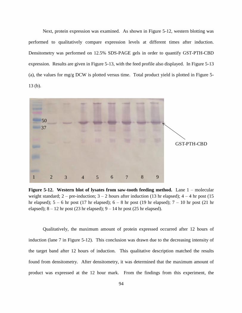
94
Next, protein expression was examined. As shown in Figure 5-12, western blotting was
performed to qualitatively compare expression levels at different times after induction.
Densitometry was performed on 12.5% SDS-PAGE gels in order to quantify GST-PTH-CBD
expression. Results are given in Figure 5-13, with the feed profile also displayed. In Figure 5-13
(a), the values for mg/g DCW is plotted versus time. Total product yield is plotted in Figure 5-
13 (b).
Figure 5-12. Western blot of lysates from saw-tooth feeding method. Lane 1 – molecular
weight standard; 2 – pre-induction; 3 – 2 hours after induction (13 hr elapsed); 4 – 4 hr post (15
hr elapsed); 5 – 6 hr post (17 hr elapsed); 6 – 8 hr post (19 hr elapsed); 7 – 10 hr post (21 hr
elapsed); 8 – 12 hr post (23 hr elapsed); 9 – 14 hr post (25 hr elapsed).
Qualitatively, the maximum amount of protein expressed occurred after 12 hours of
induction (lane 7 in Figure 5-12). This conclusion was drawn due to the decreasing intensity of
the target band after 12 hours of induction. This qualitative description matched the results
found from densitometry. After densitometry, it was determined that the maximum amount of
product was expressed at the 12 hour mark. From the findings from this experiment, the
1 2 3 4 5 6 7 8 9
50
37
GST-PTH-CBD
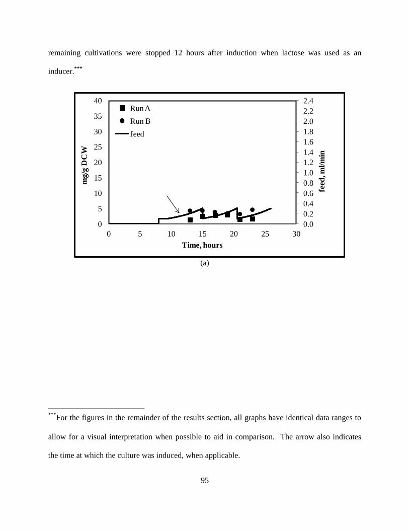
95
remaining cultivations were stopped 12 hours after induction when lactose was used as an
inducer.***
(a)
***
For the figures in the remainder of the results section, all graphs have identical data ranges to
allow for a visual interpretation when possible to aid in comparison. The arrow also indicates
the time at which the culture was induced, when applicable.
0.0
0.2
0.4
0.6
0.8
1.0
1.2
1.4
1.6
1.8
2.0
2.2
2.4
0
5
10
15
20
25
30
35
40
0 5 10 15 20 25 30
mg/g
DC
W
Time, hours
Run A
Run B
feed
feed
, ml/m
in
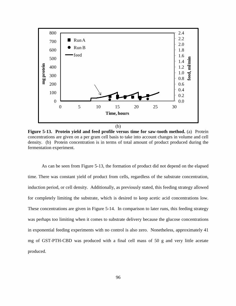
96
(b)
Figure 5-13. Protein yield and feed profile versus time for saw-tooth method. (a) Protein
concentrations are given on a per gram cell basis to take into account changes in volume and cell
density. (b) Protein concentration is in terms of total amount of product produced during the
fermentation experiment.
As can be seen from Figure 5-13, the formation of product did not depend on the elapsed
time. There was constant yield of product from cells, regardless of the substrate concentration,
induction period, or cell density. Additionally, as previously stated, this feeding strategy allowed
for completely limiting the substrate, which is desired to keep acetic acid concentrations low.
These concentrations are given in Figure 5-14. In comparison to later runs, this feeding strategy
was perhaps too limiting when it comes to substrate delivery because the glucose concentrations
in exponential feeding experiments with no control is also zero. Nonetheless, approximately 41
mg of GST-PTH-CBD was produced with a final cell mass of 50 g and very little acetate
produced.
0.0
0.2
0.4
0.6
0.8
1.0
1.2
1.4
1.6
1.8
2.0
2.2
2.4
0
100
200
300
400
500
600
700
800
0 5 10 15 20 25 30
mg
pro
tein
Time, hours
Run A
Run B
feed
feed
, ml/m
in
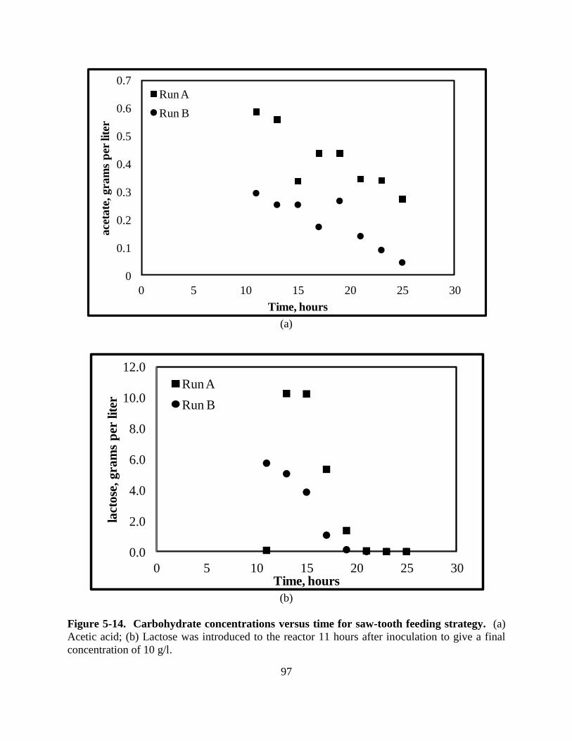
97
(a)
(b)
Figure 5-14. Carbohydrate concentrations versus time for saw-tooth feeding strategy. (a)
Acetic acid; (b) Lactose was introduced to the reactor 11 hours after inoculation to give a final
concentration of 10 g/l.
0
0.1
0.2
0.3
0.4
0.5
0.6
0.7
0 5 10 15 20 25 30
ace
tate
, g
ram
s p
er li
ter
Time, hours
Run A
Run B
0.0
2.0
4.0
6.0
8.0
10.0
12.0
0 5 10 15 20 25 30
lact
ose
, g
ram
s p
er lit
er
Time, hours
Run A
Run B

98
In an attempt to push the final cell mass to larger values, the next feeding strategy was
exponential with no adjustment or control. The growth rate was kept at 0.2 hr-1
and initial un-
induced fed-batch experiments proceeded. Four experiments were completed to monitor
accumulation of glucose in the culture broth with respect to cultivation time. The glucose
concentrations of these non-induced samples remained zero until the very end of the cultivation.
After 24 hours, accumulation of glucose at low concentrations began (less than two grams).
Because of these results, it was decided that the feeding strategy used for future fed-batch
experiments would be an exponential feeding profile with no regulatory loop and a growth rate
set at 0.2 hr-1
. It allows for limiting the substrate in fed-batch cultivations without compromising
the final total cell mass. On average for the un-induced runs, the final wet cell weight was 191
g/l with a dry cell weight of 47 g/l. Growth values were averaged and plotted versus time.
These data are shown in Figure 5-15.
Figure 5-15. Growth curve for fermentations that were un-induced using an exponential
feeding method with the growth rate set to 0.2 hr-1
.
0
10
20
30
40
50
60
70
80
0 5 10 15 20 25 30
dry
cel
l w
eigh
t, g
ram
s
Time, hours

99
The next set of experiments utilized an exponential feeding profile with a growth rate set
to 0.2 hr-1
and was induced with lactose 12 hours after inoculation.
Figure 5-16. Growth profile for fermentation experiments induced with lactose 12 hours
after inoculation. The final total dry cell weight was 60 grams. The induction period lasted for
approximately 12 hours.
The final cell mass for the exponential feeding strategy under induction with lactose was
60 grams (shown in Figure 5-16). With respect to growth, the final cell mass was not as high as
that for the un-induced control experiments, but was 10 grams higher than the final cell mass for
the saw-tooth experiments. Protein yield (mg protein/g cell) was also higher than the yield from
the experiments using the saw-tooth feeding profile. As shown in Figure 5-17 (a), the
concentration of protein produced per gram cell tripled. For the saw-tooth method, the average
protein yield was about 3 mg/g DCW, but for the exponential method the yield was almost 10
mg/g DCW. The total concentration ranged from 300 to 500 mg depending on the time at which
0
10
20
30
40
50
60
70
80
0 5 10 15 20 25 30
dry
cel
l w
eigh
t, g
ram
s
Time, hours

100
the fermentation was stopped, as shown in Figure 5-17 (b). These values increased due to the
increase in volume. On a per cell basis, the average expression of product was constant
throughout the experiment.
(a)
0.0
0.2
0.4
0.6
0.8
1.0
1.2
1.4
1.6
1.8
2.0
2.2
2.4
0.0
5.0
10.0
15.0
20.0
25.0
30.0
35.0
40.0
0 5 10 15 20 25 30
mg
/g D
CW
Time, hours
Run A
Run B
feed
feed
, ml/m
in

101
(b)
Figure 5-17. Protein concentrations for fermentations induced 12 hours after inoculation
with exponential feeding strategy. (a) Concentrations are given using a per gram cell basis;
(b) Total concentrations are calculated based on densitometry and given in milligrams.
The carbon analysis for this set of experiments (shown in Figure 5-18) yields much
information about the uptake and accumulation of substrates. Unlike the un-induced test runs,
glucose for this set of induced cultivations began to accumulate approximately 12 hours after
feeding started. This, in turn, caused accumulation of acetic acid because the glucose
consumption rate was lower than the rate at which glucose was pumped into the system (see
Section 2.3.1). Unlike the previous shake flask experiments, the lactose concentration decreased
even though glucose was present in the media. This indicates that E. coli was utilizing both
sugars simultaneously. Additionally, acetic acid concentrations began approaching inhibitory
values for one of the experiments, but growth did not appear to be stunted by this accumulation.
0.0
0.2
0.4
0.6
0.8
1.0
1.2
1.4
1.6
1.8
2.0
2.2
2.4
0
100
200
300
400
500
600
700
800
0 5 10 15 20 25 30
mg p
rote
in
Time, hours
Run A
Run B
feed
feed
, ml/m
in
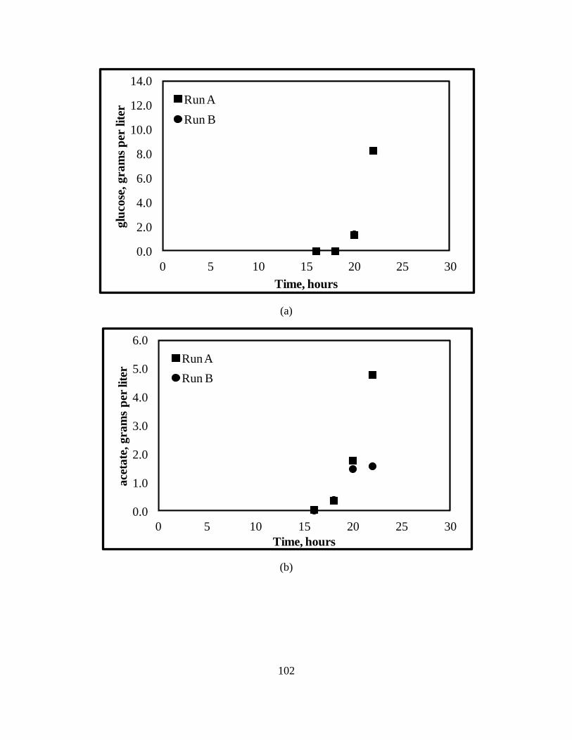
102
(a)
(b)
0.0
2.0
4.0
6.0
8.0
10.0
12.0
14.0
0 5 10 15 20 25 30
glu
cose
, gra
ms
per
lit
er
Time, hours
Run A
Run B
0.0
1.0
2.0
3.0
4.0
5.0
6.0
0 5 10 15 20 25 30
ace
tate
, g
ram
s p
er li
ter
Time, hours
Run A
Run B
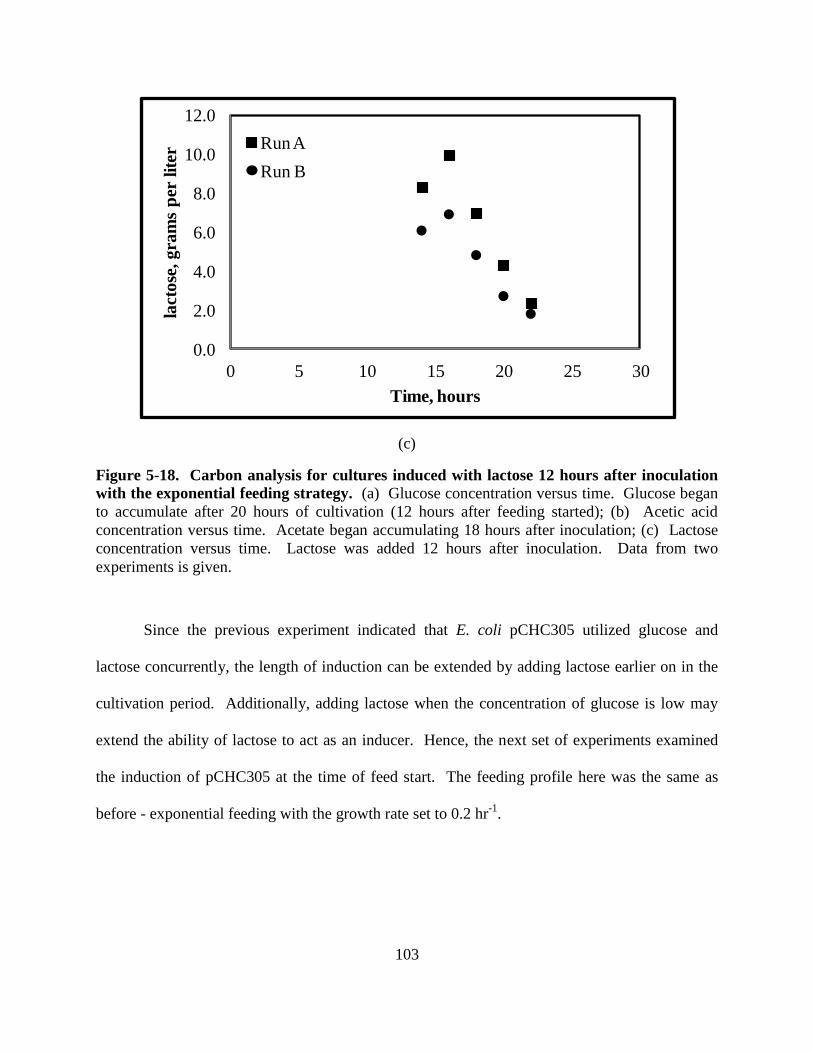
103
(c)
Figure 5-18. Carbon analysis for cultures induced with lactose 12 hours after inoculation
with the exponential feeding strategy. (a) Glucose concentration versus time. Glucose began
to accumulate after 20 hours of cultivation (12 hours after feeding started); (b) Acetic acid
concentration versus time. Acetate began accumulating 18 hours after inoculation; (c) Lactose
concentration versus time. Lactose was added 12 hours after inoculation. Data from two
experiments is given.
Since the previous experiment indicated that E. coli pCHC305 utilized glucose and
lactose concurrently, the length of induction can be extended by adding lactose earlier on in the
cultivation period. Additionally, adding lactose when the concentration of glucose is low may
extend the ability of lactose to act as an inducer. Hence, the next set of experiments examined
the induction of pCHC305 at the time of feed start. The feeding profile here was the same as
before - exponential feeding with the growth rate set to 0.2 hr-1
.
0.0
2.0
4.0
6.0
8.0
10.0
12.0
0 5 10 15 20 25 30
lact
ose
, gra
ms
per
lit
er
Time, hours
Run A
Run B
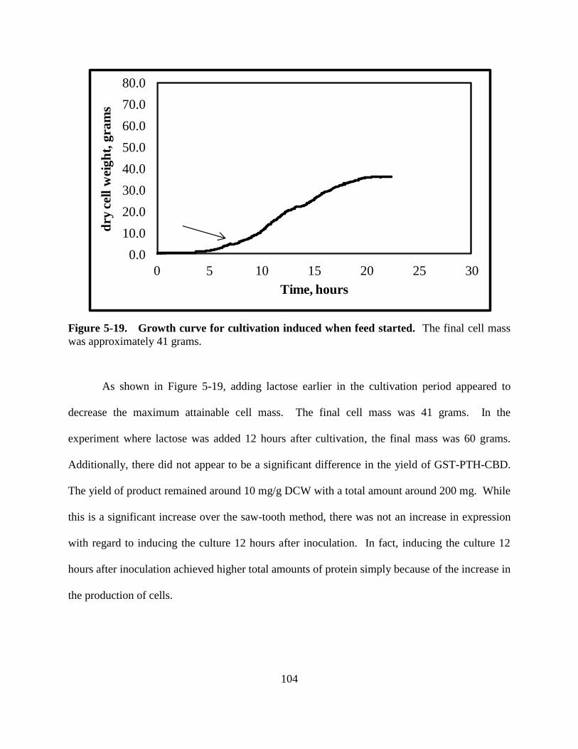
104
Figure 5-19. Growth curve for cultivation induced when feed started. The final cell mass
was approximately 41 grams.
As shown in Figure 5-19, adding lactose earlier in the cultivation period appeared to
decrease the maximum attainable cell mass. The final cell mass was 41 grams. In the
experiment where lactose was added 12 hours after cultivation, the final mass was 60 grams.
Additionally, there did not appear to be a significant difference in the yield of GST-PTH-CBD.
The yield of product remained around 10 mg/g DCW with a total amount around 200 mg. While
this is a significant increase over the saw-tooth method, there was not an increase in expression
with regard to inducing the culture 12 hours after inoculation. In fact, inducing the culture 12
hours after inoculation achieved higher total amounts of protein simply because of the increase in
the production of cells.
0.0
10.0
20.0
30.0
40.0
50.0
60.0
70.0
80.0
0 5 10 15 20 25 30
dry
cel
l w
eigh
t, g
ram
s
Time, hours
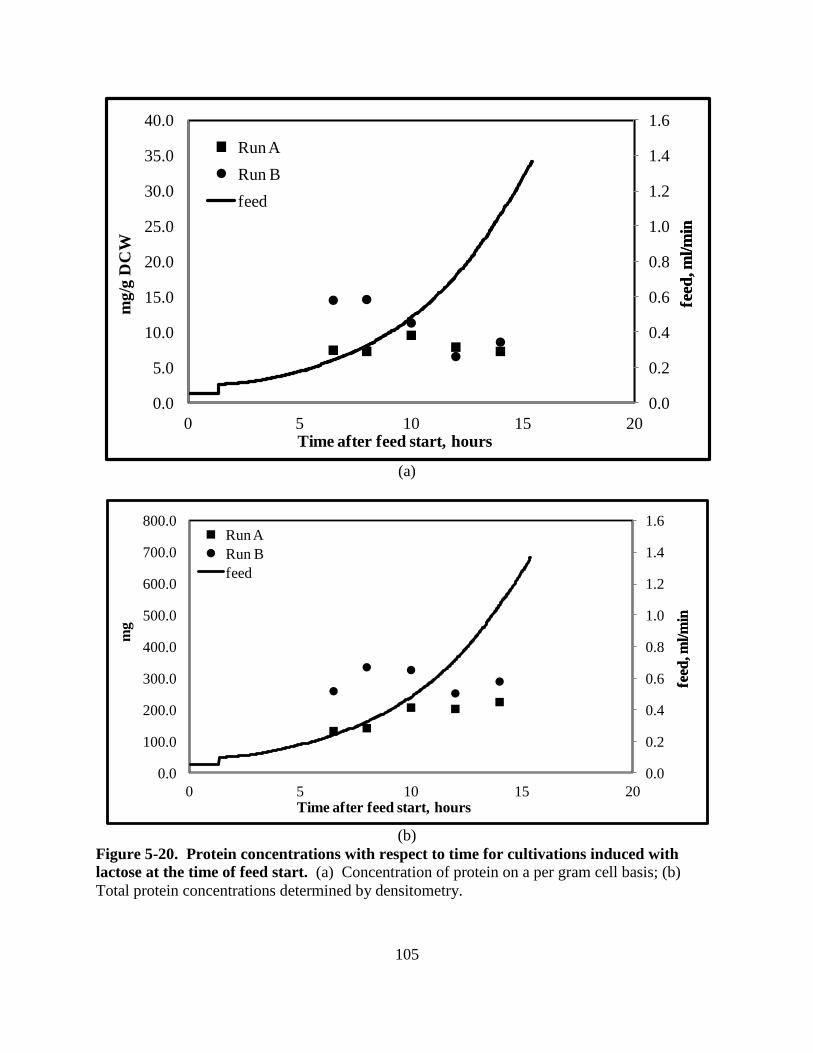
105
(a)
(b)
Figure 5-20. Protein concentrations with respect to time for cultivations induced with
lactose at the time of feed start. (a) Concentration of protein on a per gram cell basis; (b)
Total protein concentrations determined by densitometry.
0.0
0.2
0.4
0.6
0.8
1.0
1.2
1.4
1.6
0.0
5.0
10.0
15.0
20.0
25.0
30.0
35.0
40.0
0 5 10 15 20
mg
/g D
CW
Time after feed start, hours
Run A
Run B
feed
feed
, ml/
min
feed
, ml/
min
0.0
0.2
0.4
0.6
0.8
1.0
1.2
1.4
1.6
0.0
100.0
200.0
300.0
400.0
500.0
600.0
700.0
800.0
0 5 10 15 20
mg
Time after feed start, hours
Run A
Run B
feed
feed
, ml/
min
feed
, ml/
min
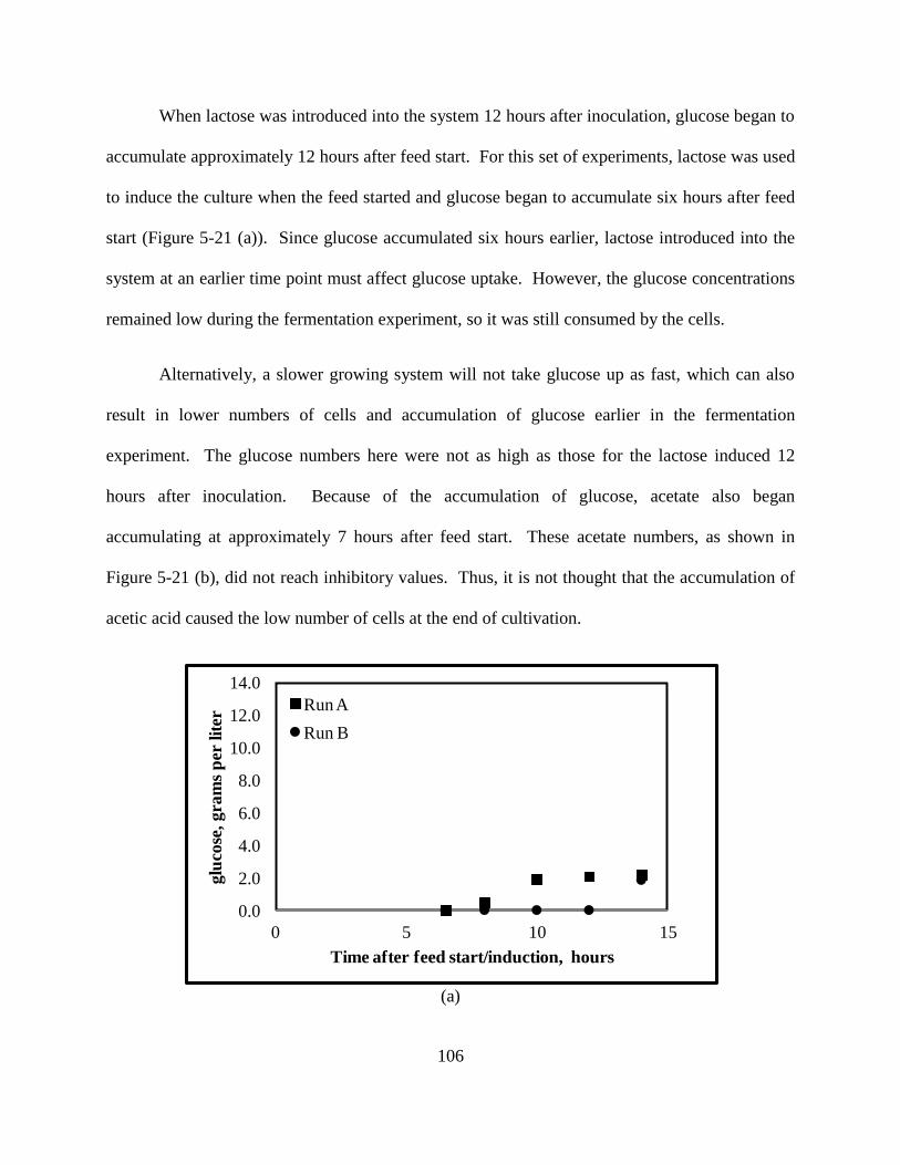
106
When lactose was introduced into the system 12 hours after inoculation, glucose began to
accumulate approximately 12 hours after feed start. For this set of experiments, lactose was used
to induce the culture when the feed started and glucose began to accumulate six hours after feed
start (Figure 5-21 (a)). Since glucose accumulated six hours earlier, lactose introduced into the
system at an earlier time point must affect glucose uptake. However, the glucose concentrations
remained low during the fermentation experiment, so it was still consumed by the cells.
Alternatively, a slower growing system will not take glucose up as fast, which can also
result in lower numbers of cells and accumulation of glucose earlier in the fermentation
experiment. The glucose numbers here were not as high as those for the lactose induced 12
hours after inoculation. Because of the accumulation of glucose, acetate also began
accumulating at approximately 7 hours after feed start. These acetate numbers, as shown in
Figure 5-21 (b), did not reach inhibitory values. Thus, it is not thought that the accumulation of
acetic acid caused the low number of cells at the end of cultivation.
(a)
0.0
2.0
4.0
6.0
8.0
10.0
12.0
14.0
0 5 10 15
glu
cose
, g
ram
s p
er lit
er
Time after feed start/induction, hours
Run A
Run B

107
(b)
(c)
Figure 5-21. Carbon analysis for cultivations induced with lactose when feed started. (a)
Glucose started to accumulate 6 hours after feed start; (b) acetic acid began to accumulate 7
hours after feed start; (c) lactose was depleted 14 hours after induction.
0.0
1.0
2.0
3.0
4.0
5.0
6.0
7.0
8.0
0 5 10 15
ace
tate
, gra
ms
per
lite
r
Time after feed start/induction, hours
Run A
Run B
0.0
1.0
2.0
3.0
4.0
5.0
6.0
7.0
8.0
0 5 10 15
lact
ose
, gra
ms
per
lit
er
Time after feed start/induction, hours
Run A
Run B

108
This specific characteristic of acetic acid concentration during fermentation has been
reported by others. Shiloach et al. (1996) compared different bacterial strains for acetic acid
consumption and inhibition. For BL21, they found that acetic acid concentrations peaked around
2 g/l. For two hours after the peak, the concentration remained constant. This was followed by a
decrease in acetic acid concentration. This outcome is very similar to the trend that is shown in
Figure 5-21 (b). Shiloach et al. proposed that the reasoning for this was because BL21 reacts to
lower acetic acid concentrations. As a result of these low concentrations, the cells reduce their
glucose uptake so acetate can be consumed.
To summarize the fed-batch fermentation experiments that utilized lactose induction at
different times with different feed profiles, Table 5-1 provides a list of experiments with their
respective results. As shown below, lactose induction 12 hours after inoculation provided the
greatest number of cells and the highest yield of protein per gram cell. However, the protein
numbers for amount produced per cell were comparable to those for fermentations that were
induced when the feed started (7 to 8.4 hours after inoculation). Of these three types of
fermentation, lactose induction 12 hours after inoculation was best at total protein production. It
is important to note that for the remaining results, YP/X describes the protein yield in terms of mg
product/g cell (dry weight).
Table 5-1. Summary of experiments performed with lactose induction (NOT auto-
induction) with glucose feed. To indicate the saw-tooth feeding profile, st is used. Other
cultivations were fed exponentially.
Method
Final DCW Average
mg
Maximum
mg
Average
YP/X
Maximum
YP/X
Lactose 11 hrs after inoc (st) 50 40.8 44.9 2.97 3.23
Lactose 12 hrs after inoc 60 327 463 9.92 11.3
Lactose at feed start 41 192 220 9.44 10.9
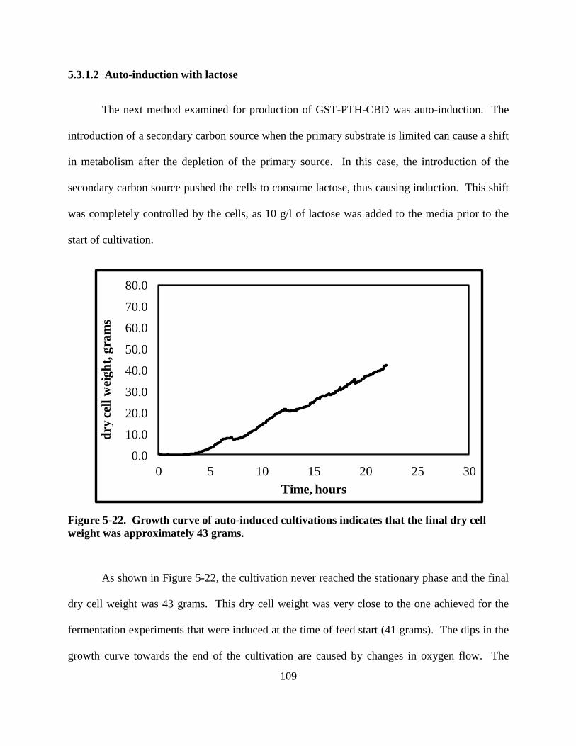
109
5.3.1.2 Auto-induction with lactose
The next method examined for production of GST-PTH-CBD was auto-induction. The
introduction of a secondary carbon source when the primary substrate is limited can cause a shift
in metabolism after the depletion of the primary source. In this case, the introduction of the
secondary carbon source pushed the cells to consume lactose, thus causing induction. This shift
was completely controlled by the cells, as 10 g/l of lactose was added to the media prior to the
start of cultivation.
Figure 5-22. Growth curve of auto-induced cultivations indicates that the final dry cell
weight was approximately 43 grams.
As shown in Figure 5-22, the cultivation never reached the stationary phase and the final
dry cell weight was 43 grams. This dry cell weight was very close to the one achieved for the
fermentation experiments that were induced at the time of feed start (41 grams). The dips in the
growth curve towards the end of the cultivation are caused by changes in oxygen flow. The
0.0
10.0
20.0
30.0
40.0
50.0
60.0
70.0
80.0
0 5 10 15 20 25 30
dry
cel
l w
eigh
t, g
ram
s
Time, hours

110
Bugeye optical density probe is sensitive to these changes, hence the reason for taking optical
density measurements by an external source throughout the cultivation.
(a)
(b)
Figure 5-23. Protein concentrations with respect to time for auto-induced cultures. (a)
Product yield; (b) Total protein concentrations.
0.0
0.2
0.4
0.6
0.8
1.0
1.2
1.4
1.6
1.8
2.0
2.2
2.4
0
5
10
15
20
25
30
35
40
0 5 10 15 20 25 30
mg
/g D
CW
Time, hours
protein
feed
feed
, ml/
min
0.0
0.2
0.4
0.6
0.8
1.0
1.2
1.4
1.6
1.8
2.0
2.2
2.4
0
100
200
300
400
500
600
700
800
0 5 10 15 20 25 30
mg p
rote
in
Time, hours
protein
feedfe
ed, m
l/m
in
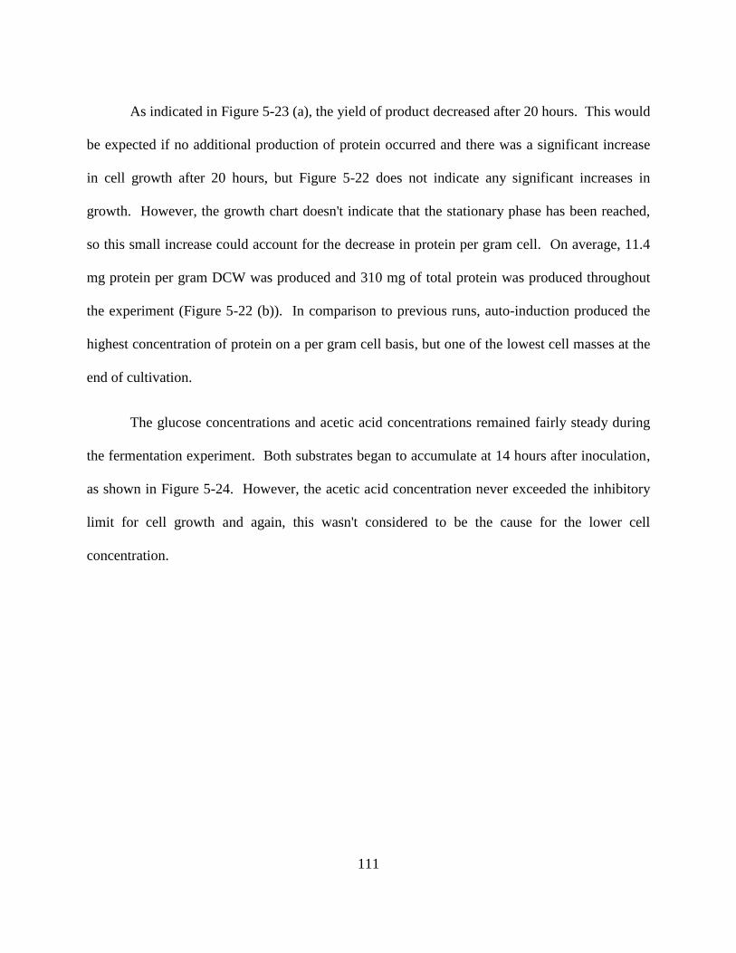
111
As indicated in Figure 5-23 (a), the yield of product decreased after 20 hours. This would
be expected if no additional production of protein occurred and there was a significant increase
in cell growth after 20 hours, but Figure 5-22 does not indicate any significant increases in
growth. However, the growth chart doesn't indicate that the stationary phase has been reached,
so this small increase could account for the decrease in protein per gram cell. On average, 11.4
mg protein per gram DCW was produced and 310 mg of total protein was produced throughout
the experiment (Figure 5-22 (b)). In comparison to previous runs, auto-induction produced the
highest concentration of protein on a per gram cell basis, but one of the lowest cell masses at the
end of cultivation.
The glucose concentrations and acetic acid concentrations remained fairly steady during
the fermentation experiment. Both substrates began to accumulate at 14 hours after inoculation,
as shown in Figure 5-24. However, the acetic acid concentration never exceeded the inhibitory
limit for cell growth and again, this wasn't considered to be the cause for the lower cell
concentration.

112
(a)
(b)
Figure 5-24. Carbohydrate concentrations for auto-induced fed-batch fermentation
experiment. (a) Glucose concentration; (b) Acetic acid concentration.
So far, it appears that lactose not only has an effect on the protein production, but also
has an effect on the final cell mass. To recap, when lactose was added 12 hours after induction,
0.0
2.0
4.0
6.0
8.0
10.0
12.0
14.0
0 5 10 15 20 25 30
glu
cose
, g
ram
s p
er lit
er
Time, hours
0.0
1.0
2.0
3.0
4.0
5.0
6.0
0 5 10 15 20 25 30
ace
tate
, gra
ms
per
lite
r
Time, hours
113
the final cell mass was 60 grams. When lactose was added when the feed started (between 7 and
8.4 hours), the final cell mass was 41 grams. Auto-induction gave a final cell mass of 43 grams.
When lactose was added earlier on in the fermentation, the cell mass was negatively affected.
After 15 hours of cultivation, the lactose concentration in the medium was less than 0.3
g/l. Because of this, the goal of the next set of experiments was to examine protein production
and cell growth using auto-induction with an additional pulse of lactose into the reactor. This
pulse was added at the 12 hour mark, as to inhibit depletion of lactose in the reactor.
Figure 5-25. Cell growth from auto-induced fermentation with lactose pulse.
The final cell mass for the auto-induced cultures with an additional lactose pulse 12 hours
after inoculation was 33 grams, as shown in Figure 5-25. This was the lowest amount of cells
produced from a fed-batch fermentation so far. Even though the cell mass suffered, product
yield actually increased and was the highest produced from any of the fed-batch fermentation
0
10
20
30
40
50
60
70
80
0 5 10 15 20 25 30
dry
cel
l w
eigh
t, g
ram
s
Time, hours
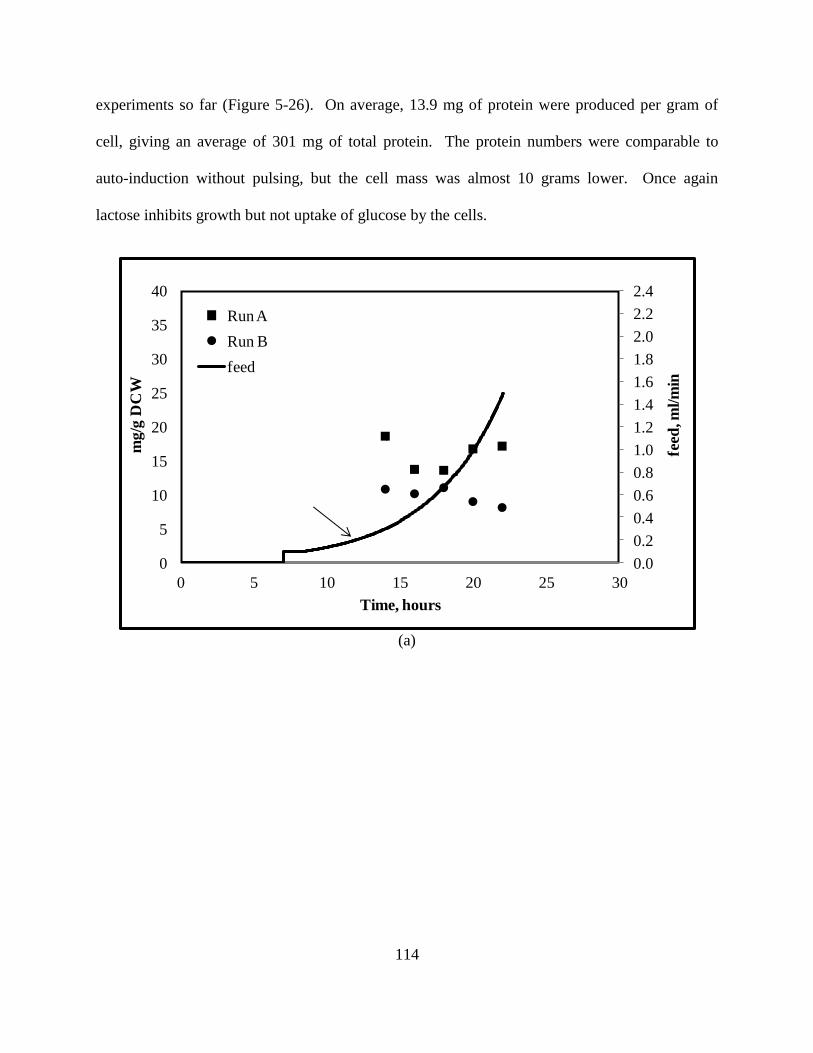
114
experiments so far (Figure 5-26). On average, 13.9 mg of protein were produced per gram of
cell, giving an average of 301 mg of total protein. The protein numbers were comparable to
auto-induction without pulsing, but the cell mass was almost 10 grams lower. Once again
lactose inhibits growth but not uptake of glucose by the cells.
(a)
0.0
0.2
0.4
0.6
0.8
1.0
1.2
1.4
1.6
1.8
2.0
2.2
2.4
0
5
10
15
20
25
30
35
40
0 5 10 15 20 25 30
mg/g
DC
W
Time, hours
Run A
Run B
feed
feed
, ml/
min
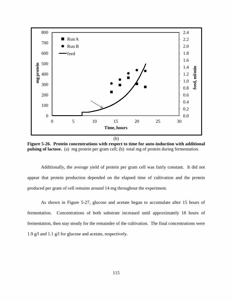
115
(b)
Figure 5-26. Protein concentrations with respect to time for auto-induction with additional
pulsing of lactose. (a) mg protein per gram cell; (b) total mg of protein during fermentation.
Additionally, the average yield of protein per gram cell was fairly constant. It did not
appear that protein production depended on the elapsed time of cultivation and the protein
produced per gram of cell remains around 14 mg throughout the experiment.
As shown in Figure 5-27, glucose and acetate began to accumulate after 15 hours of
fermentation. Concentrations of both substrate increased until approximately 18 hours of
fermentation, then stay steady for the remainder of the cultivation. The final concentrations were
1.9 g/l and 1.1 g/l for glucose and acetate, respectively.
0.0
0.2
0.4
0.6
0.8
1.0
1.2
1.4
1.6
1.8
2.0
2.2
2.4
0
100
200
300
400
500
600
700
800
0 5 10 15 20 25 30
mg p
rote
in
Time, hours
Run A
Run B
feed
feed
, ml/m
in

116
(a)
(b)
0.0
2.0
4.0
6.0
8.0
10.0
12.0
14.0
0 5 10 15 20 25 30
glu
cose
, gra
ms
per
lit
er
Time, hours
Run A
Run B
0.0
1.0
2.0
3.0
4.0
5.0
6.0
7.0
8.0
0 5 10 15 20 25 30
ace
tate
, g
ram
s p
er li
ter
Time, hours
Run A
Run B
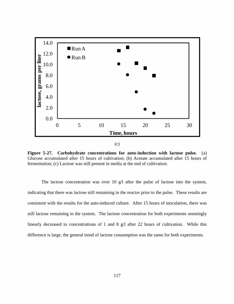
117
(c)
Figure 5-27. Carbohydrate concentrations for auto-induction with lactose pulse. (a)
Glucose accumulated after 15 hours of cultivation; (b) Acetate accumulated after 15 hours of
fermentation; (c) Lactose was still present in media at the end of cultivation.
The lactose concentration was over 10 g/l after the pulse of lactose into the system,
indicating that there was lactose still remaining in the reactor prior to the pulse. These results are
consistent with the results for the auto-induced culture. After 15 hours of inoculation, there was
still lactose remaining in the system. The lactose concentration for both experiments seemingly
linearly decreased to concentrations of 1 and 8 g/l after 22 hours of cultivation. While this
difference is large, the general trend of lactose consumption was the same for both experiments.
0.0
2.0
4.0
6.0
8.0
10.0
12.0
14.0
0 5 10 15 20 25 30
lact
ose
, gra
ms
per
lit
er
Time, hours
Run A
Run B

118
Figure 5-28. Western blot of lysates from auto-induced fed-batch cultures with lactose
pulsed into the reactor 12 hours after inoculation. Lane 1 – 2 hours post induction, run A; 2 –
4 hr after induction, run A; 3 – 6 hours after induction, run A; 4 – 8 hr post, run A; 5 – 10 hr
post, run A; 6 – molecular weight ladder; 7 – 4 hr post, run B; 8 – 6 hr post, run B; 9 – 8 hr post,
run B; 10 – 10 hr post, run B. Times of induction are given with respect to time after the pulse
into the system. For example, 6 hours post would be 18 hours after inoculation since the pulse
was added 12 hours after inoculation.
As shown by the western blot in Figure 5-28, intense bands representing target protein
are present in samples of lysates taken throughout the fermentation experiment. The lysates are
from two separate experiments. In run A (left of the molecular ladder), the highest concentration
of target protein was produced 8 hours after the pulse of lactose into the system. On the other
hand, for run B (right of the molecular ladder), the highest concentration of target protein was
produced after only 4 hours of induction with respect to the pulse of lactose. However, the
average amount of product remains somewhat constant according to the densitometry results
given in Figure 5-26 (b).

119
5.3.1.3 IPTG induction
To establish a comparison for the lactose-induced runs, experiments were set up for IPTG
induction. One set was induced with IPTG to a final concentration of 5 mM. The second set
was induced with IPTG to a final concentration of 10 mM. In both cases, the desired induction
period was five hours. To induce the maximum number of cells, IPTG was added to the reactor
19 hours after inoculation and the experiment was stopped 24 hours after inoculation. Glucose
was utilized as the feed in both cases.
Figure 5-29. Growth curve for 5 mM IPTG-induced culture.
The final dry cell weight for cultivations induced with 5 mM IPTG exceeded previous
experiments. With a final dry cell weight of 76 grams (Figure 5-29), these cultivations surpassed
the 12 hour lactose cultivations by 16 grams. Additionally, the stationary phase of growth was
0
10
20
30
40
50
60
70
80
0 5 10 15 20 25 30
dry
cell
weig
ht
Time, hours

120
not achieved, even after 24 hours of cultivation. Thus, on the fed-batch level, IPTG did not
affect cell growth. This result was not expected. As shown previously (Figure 5-10), IPTG
negatively affected growth on the batch scale. Also, others reported on growth inhibition by
IPTG. Kilikian et al. (2000) found that cell yield from glucose using lactose as an inducer was
four times higher than the cultures that were induced with IPTG. Contrary to what Kilikian et al.
(2000) and Kosinski et al. (1992) report, there was no apparent metabolic burden from IPTG
induction on the fed-batch scale. Also, protein expression with IPTG did occur, so protein
production from IPTG did not place any apparent burden on cell growth.
(a)
0.0
0.2
0.4
0.6
0.8
1.0
1.2
1.4
1.6
1.8
2.0
2.2
2.4
0
5
10
15
20
25
30
35
40
0 5 10 15 20 25 30
mg/g
DC
W
Time, hours
Run A
Run B
feed
feed
, ml/m
in

121
(b)
Figure 5-30. Protein concentrations with respect to time for 5 mM IPTG-induced
cultivations. (a) Protein expression on a per gram cell basis; (b) Total amount of protein
expressed during cultivation with IPTG induction.
As shown in Figure 5-30 (a), the average product yield was approximately 9 mg. This
yield was actually lower that that achieved from auto-induced cultures and comparable to that
achieved from simple lactose induction. Though, the yield of protein per cell remained constant
for both experiments, which is a similar characteristic to most of the lactose-induced experiments
previously discussed. On a per gram cell level, auto-induced cultures on defined medium
surpassed protein production from IPTG-induced cultures. However, 5 mM IPTG induction
surpassed lactose induction and auto-induction with regard to total protein expression. This is
due to the higher cell densities that were attained using IPTG as an inducer. The average total
amount of protein expressed under IPTG induction was approximately 540 mg (Figure 5-30 (b)).
The maximum amount of total protein approached 700 mg and was expressed 4 hours after IPTG
induction.
0.0
0.2
0.4
0.6
0.8
1.0
1.2
1.4
1.6
1.8
2.0
2.2
2.4
0
100
200
300
400
500
600
700
800
0 5 10 15 20 25 30
mg
pro
tein
Time, hours
Run A
Run B
feed
feed
, ml/m
in
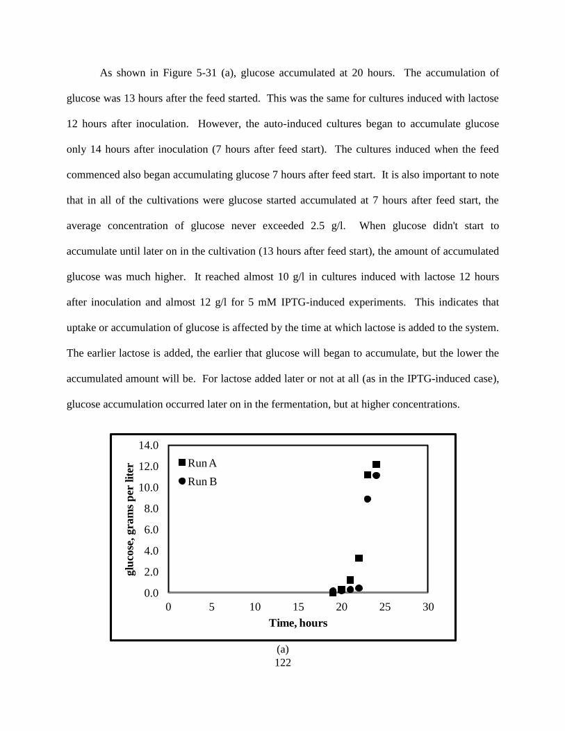
122
As shown in Figure 5-31 (a), glucose accumulated at 20 hours. The accumulation of
glucose was 13 hours after the feed started. This was the same for cultures induced with lactose
12 hours after inoculation. However, the auto-induced cultures began to accumulate glucose
only 14 hours after inoculation (7 hours after feed start). The cultures induced when the feed
commenced also began accumulating glucose 7 hours after feed start. It is also important to note
that in all of the cultivations were glucose started accumulated at 7 hours after feed start, the
average concentration of glucose never exceeded 2.5 g/l. When glucose didn't start to
accumulate until later on in the cultivation (13 hours after feed start), the amount of accumulated
glucose was much higher. It reached almost 10 g/l in cultures induced with lactose 12 hours
after inoculation and almost 12 g/l for 5 mM IPTG-induced experiments. This indicates that
uptake or accumulation of glucose is affected by the time at which lactose is added to the system.
The earlier lactose is added, the earlier that glucose will began to accumulate, but the lower the
accumulated amount will be. For lactose added later or not at all (as in the IPTG-induced case),
glucose accumulation occurred later on in the fermentation, but at higher concentrations.
(a)
0.0
2.0
4.0
6.0
8.0
10.0
12.0
14.0
0 5 10 15 20 25 30
glu
cose
, g
ram
s p
er lit
er
Time, hours
Run A
Run B

123
(b)
Figure 5-31. Carbohydrate analysis for 5 mM IPTG-induced cultures. (a) Glucose
concentrations; (b) Acetic acid concentrations. Data from two different experiments is given.
As previously witnessed, acetic acid began to accumulate approximately when glucose
began accumulating. Once again, the amounts of acetic acid accumulation (Figure 5-31 (b)) did
not exceed the inhibitory value. In fact, the concentration of acetic acid remained under one
gram per liter even though glucose accumulated in high amounts.
Next, induction with 10 mM IPTG was examined. It was suggested that 10 mM IPTG be
used to induce protein expression with this particular construct, so this experiment was
performed as a baseline comparison for lactose-induced runs in the same manner that the 5 mM
IPTG-induced experiments were conducted. The growth for 10 mM IPTG-induced runs was
very similar to that for 5 mM IPTG induction and is shown in Figure 5-32. Because these
fermentations never reached the stationary phase, it can be conjectured that the fermentation
could be induced at a later time to produce even more protein. Also, 10 mM IPTG-induced
0.0
1.0
2.0
3.0
4.0
5.0
6.0
0 5 10 15 20 25 30
ace
tate
, gra
ms
per
lite
r
Time, hours
Run A
Run B
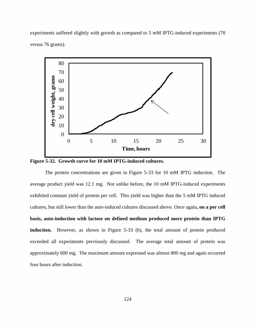
124
experiments suffered slightly with growth as compared to 5 mM IPTG-induced experiments (70
versus 76 grams).
Figure 5-32. Growth curve for 10 mM IPTG-induced cultures.
The protein concentrations are given in Figure 5-33 for 10 mM IPTG induction. The
average product yield was 12.1 mg. Not unlike before, the 10 mM IPTG-induced experiments
exhibited constant yield of protein per cell. This yield was higher than the 5 mM IPTG induced
cultures, but still lower than the auto-induced cultures discussed above. Once again, on a per cell
basis, auto-induction with lactose on defined medium produced more protein than IPTG
induction. However, as shown in Figure 5-33 (b), the total amount of protein produced
exceeded all experiments previously discussed. The average total amount of protein was
approximately 600 mg. The maximum amount expressed was almost 800 mg and again occurred
four hours after induction.
0
10
20
30
40
50
60
70
80
0 5 10 15 20 25 30
dry
cel
l w
eigh
t, g
ram
s
Time, hours

125
(a)
(b)
Figure 5-33. Protein concentrations with respect to time for 10 mM IPTG-induced
cultures.
0.0
0.2
0.4
0.6
0.8
1.0
1.2
1.4
1.6
1.8
2.0
2.2
2.4
0
5
10
15
20
25
30
35
40
0 5 10 15 20 25 30
mg
/g D
CW
Time, hours
Run A
Run B
feed
feed
, ml/m
in
0.0
0.2
0.4
0.6
0.8
1.0
1.2
1.4
1.6
1.8
2.0
2.2
2.4
0
100
200
300
400
500
600
700
800
0 5 10 15 20 25 30
mg
pro
tein
Time, hours
Run A
Run B
feed
feed
, ml/m
in

126
The carbohydrate analysis for the 10 mM IPTG-induced experiments mimicked that for
the 5 mM IPTG-induced experiments. Glucose accumulated approximately 20 hours after
inoculation, as shown in Figure 5-34 (a), to almost 12 g/l for both experiments. This was the
same time and concentration at which glucose accumulated for the 5 mM IPTG induction
experiments. Similarly, acetic acid accumulated to 1 g/l, which is well below the value thought
to inhibit cell growth (Figure 5-34 (b)).
(a)
0.0
2.0
4.0
6.0
8.0
10.0
12.0
14.0
0 5 10 15 20 25 30
glu
cose
, gra
ms
per
lit
er
Time, hours
Run A
Run B
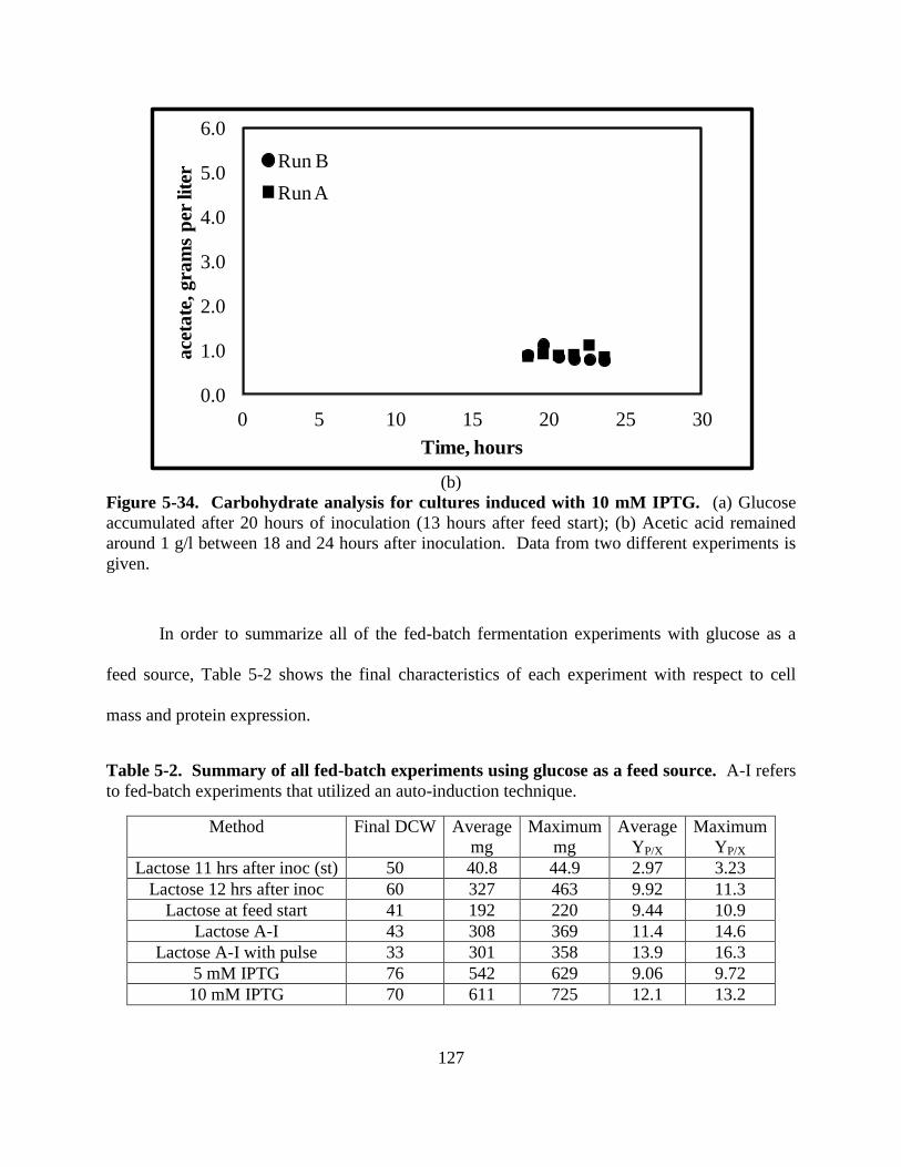
127
(b)
Figure 5-34. Carbohydrate analysis for cultures induced with 10 mM IPTG. (a) Glucose
accumulated after 20 hours of inoculation (13 hours after feed start); (b) Acetic acid remained
around 1 g/l between 18 and 24 hours after inoculation. Data from two different experiments is
given.
In order to summarize all of the fed-batch fermentation experiments with glucose as a
feed source, Table 5-2 shows the final characteristics of each experiment with respect to cell
mass and protein expression.
Table 5-2. Summary of all fed-batch experiments using glucose as a feed source. A-I refers
to fed-batch experiments that utilized an auto-induction technique.
Method Final DCW Average
mg
Maximum
mg
Average
YP/X
Maximum
YP/X
Lactose 11 hrs after inoc (st) 50 40.8 44.9 2.97 3.23
Lactose 12 hrs after inoc 60 327 463 9.92 11.3
Lactose at feed start 41 192 220 9.44 10.9
Lactose A-I 43 308 369 11.4 14.6
Lactose A-I with pulse 33 301 358 13.9 16.3
5 mM IPTG 76 542 629 9.06 9.72
10 mM IPTG 70 611 725 12.1 13.2
0.0
1.0
2.0
3.0
4.0
5.0
6.0
0 5 10 15 20 25 30
ace
tate
, g
ram
s p
er li
ter
Time, hours
Run B
Run A

128
According to Table 5-2, IPTG-induction yielded the highest amount of total protein. This
finding is due to the fact that higher cell densities were achieved using IPTG as an inducer.
However, experiments that utilized an auto-induction technique yielded the highest amount of
protein per gram of cell. It is also important to note that IPTG did not have an effect on growth
on the 3L fed-batch scale, as it did on the batch scale. Since batch cultures were also induced
with 5 mM and 10 mM IPTG, this was not expected. However, for batch cultivations, induction
occurred when the optical density was less than 6 units. For fed-batch cultivations, induction
occurred when the optical density was between 65-70 units. This is a 10-fold difference in cell
density and on a per cell basis, the cells in the batch cultivations witnessed higher local IPTG
concentrations. Since the amount of IPTG added is based only on volume (not on cell density),
this local concentration difference may account for the differences in IPTG affecting growth.
Also, as shown in the growth curves for fed-batch experiments utilizing lactose, lactose inhibited
the production of biomass, but not the uptake of glucose on the fed-batch scale.
5.3.2 Cultures fed with glycerol as major carbon source
5.3.2.1 Lactose induction after inoculation (at feed start)
To investigate the ability of lactose to act as an inducer in the absence of glucose, fed-
batch experiments were performed with glycerol feed. The first experiment utilized a pulsing of
15 grams of lactose into the system when the feed commenced. 15 grams of lactose was used
instead of 10 g/l to see if the higher amount of lactose increased the amount of product with no
substrate inhibition due to the presence of glucose in the system. The initial concentration of
lactose after the pulse was approximately 14 g/l. As shown in Figure 5-35, the final dry cell

129
weight barely reached 20 grams. This was the lowest final dry cell weight observed amongst all
of the experiments thus far.
Figure 5-35. Growth chart for glycerol-fed cultivations with 15 grams lactose added at feed
start.
Even though the final cell mass was low, the product yield was comparable to that
achieved in the experiments that were auto-induced and pulsed with lactose. The average yield
per gram cell was 13.7 mg/g DCW (shown in Figure 5-36 (a)). This was one of the highest
numbers reached for yield of product per gram cell. Also, the yield of product actually increased
during the fermentation experiment. In previous experiments, the yield remained somewhat
constant or oscillated during the experiment. The maximum yield achieved in this run was 16.2
mg/g DCW. The highest maximum yield was achieved in the auto-induced pulsed with lactose
experiment at an average value of 16.3 mg/g DCW. Thus, protein yield numbers from glycerol-
fed auto-induced experiments mimicked those achieved from auto-inducting cultures using
glucose as the feed substrate with an extra lactose pulse.
0
10
20
30
40
50
60
70
80
0 5 10 15 20 25 30
dry
cel
l w
eigh
t, g
ram
s
Time, hours

130
(a)
(b)
Figure 5-36. Protein concentration with respect to time for glycerol-fed cultivations with
15 grams of lactose added at feed start. (a) Protein produced per gram cell; (b) Total protein
production.
0.0
0.2
0.4
0.6
0.8
1.0
1.2
1.4
1.6
1.8
2.0
2.2
2.4
0
5
10
15
20
25
30
35
40
0 5 10 15 20 25 30
mg/g
DC
W
Time, hours
Run ARun Bfeed
feed
, ml/
min
0.0
0.2
0.4
0.6
0.8
1.0
1.2
1.4
1.6
1.8
2.0
2.2
2.4
0
100
200
300
400
500
600
700
800
0 5 10 15 20 25 30
mg p
rote
in
Time, hours
Run A
Run B
feed
feed
, ml/
min
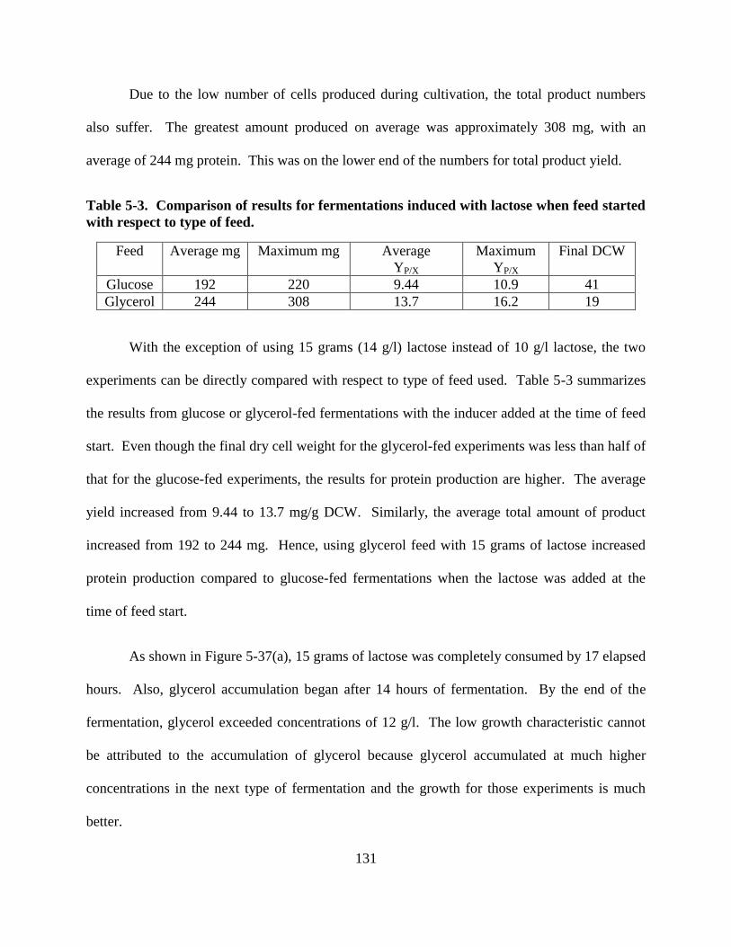
131
Due to the low number of cells produced during cultivation, the total product numbers
also suffer. The greatest amount produced on average was approximately 308 mg, with an
average of 244 mg protein. This was on the lower end of the numbers for total product yield.
Table 5-3. Comparison of results for fermentations induced with lactose when feed started
with respect to type of feed.
Feed Average mg Maximum mg Average
YP/X
Maximum
YP/X
Final DCW
Glucose 192 220 9.44 10.9 41
Glycerol 244 308 13.7 16.2 19
With the exception of using 15 grams (14 g/l) lactose instead of 10 g/l lactose, the two
experiments can be directly compared with respect to type of feed used. Table 5-3 summarizes
the results from glucose or glycerol-fed fermentations with the inducer added at the time of feed
start. Even though the final dry cell weight for the glycerol-fed experiments was less than half of
that for the glucose-fed experiments, the results for protein production are higher. The average
yield increased from 9.44 to 13.7 mg/g DCW. Similarly, the average total amount of product
increased from 192 to 244 mg. Hence, using glycerol feed with 15 grams of lactose increased
protein production compared to glucose-fed fermentations when the lactose was added at the
time of feed start.
As shown in Figure 5-37(a), 15 grams of lactose was completely consumed by 17 elapsed
hours. Also, glycerol accumulation began after 14 hours of fermentation. By the end of the
fermentation, glycerol exceeded concentrations of 12 g/l. The low growth characteristic cannot
be attributed to the accumulation of glycerol because glycerol accumulated at much higher
concentrations in the next type of fermentation and the growth for those experiments is much
better.
132
The acetic acid concentration in this type of fermentation did not exceed 0.4 g/l (Figure
5-37(b)) and was oscillatory in nature. It first began accumulating when glycerol began to
accumulate. However, the glycerol accumulated in an exponential manner for both experiments,
while acetate decreased at the next time point. This was followed by an increase. Because of the
low concentration of acetic acid, the low density of cells cannot be attributed to growth inhibition
by acetate. However, it was not expected that acetic acid will accumulate in glycerol-fed
cultivations. The reasoning for this accumulation is discussed in detail in the next section.
(a)
0
2
4
6
8
10
12
14
0
0.5
1
1.5
2
2.5
3
3.5
4
10 11 12 13 14 15 16 17 18
lact
ose
, g
ram
s p
er lit
er
Time, hours
Lactose A
Lactose B
Glycerol A
Glycerol B
gly
cero
l, g
ram
sp
er lit
er

133
(b)
Figure 5-37. Carbon concentrations with respect to time for glycerol-fed cultivations
induced with 15 grams of lactose at feed start. (a) Lactose and glycerol concentrations during
fermentation; (b) acetic acid concentrations during cultivation.
It is important to note that there were only three data points for the protein concentrations
for these experiments because foam became an issue with glycerol-fed fermentations that were
induced when the feed began. On multiple occasions, disregarding the high concentration of
anti-foam in the reactor, the culture broth foamed out of the reactor through the condenser
exhaust tube. This event happened after 17 hours of fermentation on each occasion. It could be
conjectured that higher amounts of protein would have been produced if the fermentation
experiment had lasted for longer than 17 hours. However, 17 hours of fermentation time did
allow for a ten hour induction period which is consistent with previous experiments. Also, since
the stationary phase had been reached almost five hours prior to foaming-out, cell growth
probably would not have benefited from additional fermentation time.
0.0
1.0
2.0
3.0
4.0
5.0
6.0
0 5 10 15 20 25 30
ace
tate
, gra
ms
per
lite
r
Time, hours
Run A
Run B

134
From a cost stand point, the cost of production of these two experiments is also
comparable. About six cents separates the cost per mg/g DCW of product, with the lower
amount coming from the glucose-fed experiment. The cost analysis is discussed for each
experiment in detail in Section 5.4.
5.3.2.2 Auto-induction with lactose
The next set of experiments examined auto-induction with glycerol. Lactose was added
prior to inoculation at a concentration of 10 g/l. As shown in Figure 5-38, the final dry cell
weight was approximately 35 grams. This was almost double the dry cell weight from the
fermentations using glycerol feed and induction with lactose at feed start, but half as much as the
glucose-fed IPTG-induced fermentation experiments.
Figure 5-38. Growth chart for auto-induced cultures with glycerol feed.
0
10
20
30
40
50
60
70
80
0 5 10 15 20 25 30
dry
cel
l w
eig
ht,
gra
ms
Time, hours

135
Even though the final cell mass did not exceed experiments previously performed,
protein yield exceeded any fermentation thus far. As shown in Figure 5-39 (a), the production of
protein remained somewhat constant throughout the fermentation experiment at an average value
of 20.2 mg/g DCW. (The next highest is 13.9 mg/g DCW and was achieved in the auto-induced
glucose-fed experiments with an extra pulse of lactose.) The total protein numbers increased
linearly (Figure 5-39 (b)) during the experiment due to the fact that the stationary phase never
completely leveled off or remained constant, as shown in Figure 5-38. The average maximum
total amount of protein produced was 522 mg, with an overall average amount of 426 mg.
(a)
0.0
0.2
0.4
0.6
0.8
1.0
1.2
1.4
1.6
0.0
5.0
10.0
15.0
20.0
25.0
30.0
35.0
40.0
0 5 10 15 20 25 30
mg/g
DC
W
Time, hours
Run A
Run B
feed
feed
, ml/
min

136
(b)
Figure 5-39. Protein concentrations with respect to time for auto-induced cultures with
glycerol feed.
For cultures auto-induced with lactose, direct comparison of results is feasible since the
only difference between the two sets of experiments is the feed type. Table 5-4 summarizes the
important results with respect to protein production and final dry cell weight based on the
feeding substrate. For glucose-fed auto-induced cultures, the final dry cell weight was slightly
higher. However, the glycerol-fed auto-induced cultures produced almost two times the amount
of GST-PTH-CBD than the glucose-fed fermentations. Though, unlike before, the cost of
producing 1 mg/g DCW using auto-induced glycerol-fed cultures was double that of auto-
induced glucose-fed cultivations. As discussed later in Section 5.4, this cost is still extremely
low compared to cultures that were induced with IPTG ($0.185 and $0.36 versus $5.97).
0.0
0.2
0.4
0.6
0.8
1.0
1.2
1.4
1.6
1.8
2.0
2.2
2.4
0
100
200
300
400
500
600
700
800
0 5 10 15 20 25 30
mg
pro
tein
Time, hours
Run A
Run B
feed
feed
, ml/m
in

137
Table 5-4. Comparison of auto-induced experiments with respect to feed type.
Feed Average mg Average
maximum mg
Average
YP/X
Maximum
YP/X
Final DCW
Glucose 308 369 11.4 14.6 43
Glycerol 426 522 20.2 22.0 35
In these experiments, the lactose was completely depleted by 15 hours. Glycerol also
accumulated 15 hours after inoculation, as shown in Figure 5-40(a). The glycerol concentration
at the 17 hour mark was similar to that in the 17 hour sample from the previous glycerol-fed
fermentation with lactose added at feed start. But, since this fermentation experiment lasted four
hours longer, the final glycerol concentration exceeded 50 g/l. The highest concentration of
substrate accumulated in the glucose-fed experiments was approximately 12 g/l. It is clear
through these experiments that the cells do not consume glycerol as efficiently as they consume
glucose with the feed profile that was in use. This was expected due to the lower growth rates
and lower biomass yields that are typically found in the literature when using glycerol feed
(compared to glucose feed). Also, glycerol could have become inhibiting over a certain amount,
though the concentration here did not exceed the reported inhibitory value. Glycerol
accumulated at concentrations greater than 10g/l around 17 hours after inoculation. This was
approximately when the stationary phase of the culture is reached (Figure 5-38).
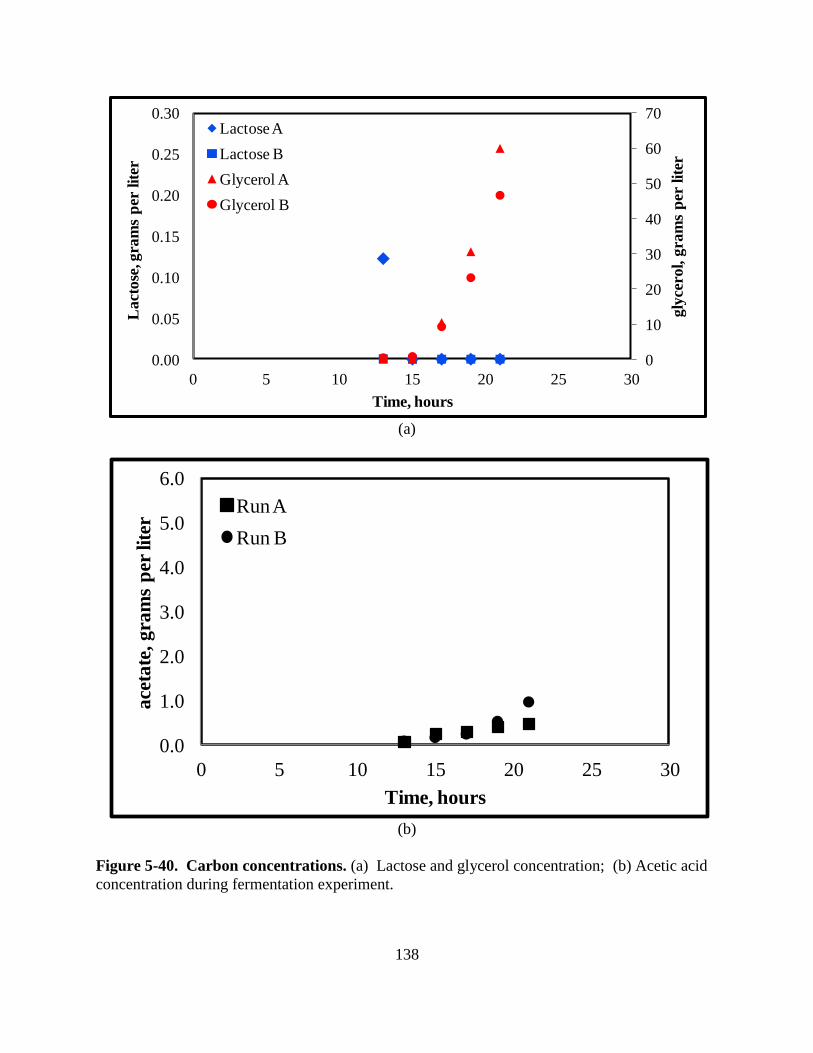
138
(a)
(b)
Figure 5-40. Carbon concentrations. (a) Lactose and glycerol concentration; (b) Acetic acid
concentration during fermentation experiment.
0
10
20
30
40
50
60
70
0.00
0.05
0.10
0.15
0.20
0.25
0.30
0 5 10 15 20 25 30
Lact
ose
, gra
ms
per
lit
er
Time, hours
Lactose A
Lactose B
Glycerol A
Glycerol B
gly
cero
l, g
ram
s p
er lit
er
0.0
1.0
2.0
3.0
4.0
5.0
6.0
0 5 10 15 20 25 30
ace
tate
, gra
ms
per
lite
r
Time, hours
Run A
Run B
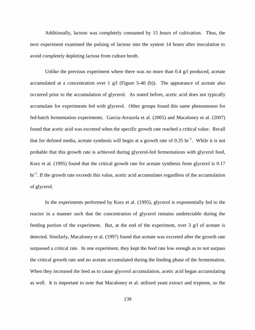
139
Additionally, lactose was completely consumed by 15 hours of cultivation. Thus, the
next experiment examined the pulsing of lactose into the system 14 hours after inoculation to
avoid completely depleting lactose from culture broth.
Unlike the previous experiment where there was no more than 0.4 g/l produced, acetate
accumulated at a concentration over 1 g/l (Figure 5-40 (b)). The appearance of acetate also
occurred prior to the accumulation of glycerol. As stated before, acetic acid does not typically
accumulate for experiments fed with glycerol. Other groups found this same phenomenon for
fed-batch fermentation experiments. Garcia-Arrazola et al. (2005) and Macaloney et al. (2007)
found that acetic acid was excreted when the specific growth rate reached a critical value. Recall
that for defined media, acetate synthesis will begin at a growth rate of 0.35 hr-1
. While it is not
probable that this growth rate is achieved during glycerol-fed fermentations with glycerol feed,
Korz et al. (1995) found that the critical growth rate for acetate synthesis from glycerol is 0.17
hr-1
. If the growth rate exceeds this value, acetic acid accumulates regardless of the accumulation
of glycerol.
In the experiments performed by Korz et al. (1995), glycerol is exponentially fed to the
reactor in a manner such that the concentration of glycerol remains undetectable during the
feeding portion of the experiment. But, at the end of the experiment, over 3 g/l of acetate is
detected. Similarly, Macaloney et al. (1997) found that acetate was excreted after the growth rate
surpassed a critical rate. In one experiment, they kept the feed rate low enough as to not surpass
the critical growth rate and no acetate accumulated during the feeding phase of the fermentation.
When they increased the feed as to cause glycerol accumulation, acetic acid began accumulating
as well. It is important to note that Macaloney et al. utilized yeast extract and tryptone, so the

140
media was not completely defined. However, Garcia-Arrazola et al. (2005) utilized a completely
defined media and found similar results.
It can be concluded that acetate does accumulate when glycerol is used as the carbon
source if a certain critical growth rate is reached. Though, the concentration of acetate that
accumulated for this experiment was low compared to the concentration that must be reached to
cause inhibition of growth.
The final fermentation that was performed utilized auto-induction with an additional
pulse of lactose into the system 14 hours after inoculation. Ten grams of lactose was added prior
to inoculation. As shown in Figure 5-41, the final cell mass never exceeded 20 grams. The
growth for this experiment was comparable to the glycerol-fed fermentations with lactose added
at the time that feeding began. The stationary phase was reached early on in the cultivation -
only 12 hours after inoculation. The fermentation was carried out for nine additional hours and a
slight increase in growth was witnessed towards the end of run. However, the final dry cell
weight was still among the lowest dry cell weights achieved for a fed-batch fermentation
experiment.

141
Figure 5-41. Growth curve for auto-induced cultures with lactose pulsed into glycerol-fed
fermentation at 14 hours.
The trends for product yield are interesting for auto-induction with a pulse and glycerol
feed. As shown in Figure 5-42 (a), an increase in product formation was witnessed from 13 to 17
hours after inoculation. After this point, a decline in product occurred. This was the only
experiment where the increase in product yield per gram of cells was followed by a sharp
decline. This would make sense if there was a sharp increase in the number of cells and constant
product formation because the division of product by a larger number would decrease product
per gram cell. As previously discussed, a slight increase towards the very end of the experiment
occurred, but it was not significant enough to decrease the product yield as such.
At its maximum, 16.3 mg/g DCW of target protein was made. On average, 12.1 mg/g
DCW of GST-PTH-CBD was produced. This was the same per gram cell yield as that for
0
10
20
30
40
50
60
70
80
0 5 10 15 20 25 30
dry
cel
l w
eig
ht,
gra
ms
Time, hours

142
cultures induced with 10 mM IPTG. Due to the lack of accumulation of cell mass, the total
protein numbers were quite low. With the exception of the total protein from the saw-tooth
cultivations, they were the lowest achieved in all fermentation experiments. 177 mg of GST-
PTH-CBD was produced, as shown in Figure 5-42 (b). On average, approximately 150 mg of
protein was made during each cultivation experiment.
(a)
0.0
0.2
0.4
0.6
0.8
1.0
1.2
1.4
1.6
0
5
10
15
20
25
30
35
40
0 5 10 15 20 25 30
mg
/g D
CW
Time, hours
protein
feed
feed
, ml/m
in
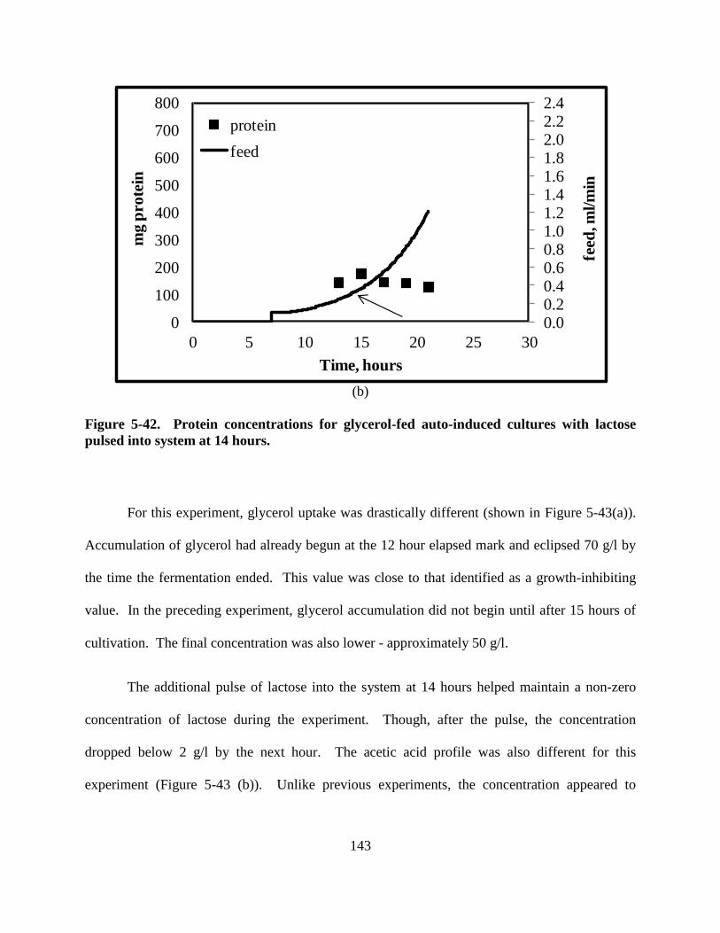
143
(b)
Figure 5-42. Protein concentrations for glycerol-fed auto-induced cultures with lactose
pulsed into system at 14 hours.
For this experiment, glycerol uptake was drastically different (shown in Figure 5-43(a)).
Accumulation of glycerol had already begun at the 12 hour elapsed mark and eclipsed 70 g/l by
the time the fermentation ended. This value was close to that identified as a growth-inhibiting
value. In the preceding experiment, glycerol accumulation did not begin until after 15 hours of
cultivation. The final concentration was also lower - approximately 50 g/l.
The additional pulse of lactose into the system at 14 hours helped maintain a non-zero
concentration of lactose during the experiment. Though, after the pulse, the concentration
dropped below 2 g/l by the next hour. The acetic acid profile was also different for this
experiment (Figure 5-43 (b)). Unlike previous experiments, the concentration appeared to
0.00.20.40.60.81.01.21.41.61.82.02.22.4
0
100
200
300
400
500
600
700
800
0 5 10 15 20 25 30
mg p
rote
in
Time, hours
protein
feed
feed
, ml/
min

144
decrease as glycerol accumulated. Towards the end of the fermentation, it leveled off and then
decreased drastically in the final sample taken.
As before, the accumulation of glycerol at such a high amount shows how inefficiently
the cells uptake glycerol when the same exponential feed profile used for glucose feed is used for
feeding glycerol. It could be that this high concentration of glycerol becomes the inhibitory
factor for growth. This could account for the stationary phase being reached at 12 hours after
inoculation.
(a)
0
10
20
30
40
50
60
70
80
0
0.5
1
1.5
2
2.5
0 5 10 15 20 25 30
La
cto
se, g
ram
s p
er lit
er
Time, hours
lactose
glycerol
gly
cero
l, g
ram
s p
er lit
er

145
(b)
Figure 5-43. Carbon concentrations for glycerol-fed auto-induced cultures with lactose
pulsed into system at 14 hours. (a) Lactose and glycerol concentrations; (b) acetic acid
concentrations during fermentation.
As shown in Table 5-5, the final cell mass for auto-induced cultures with an extra pulse
of lactose (and fed with glycerol) was extremely low compared to the cultures fed with glucose.
However, the maximum amount of protein produced per gram of cell was practically the same.
Though, the average amount for glycerol-fed cultures was slightly lower. The total amounts
were also extremely different. Less than half of the total product for glucose-fed experiments
was produced in glycerol-fed experiments. As stated above, this was due to the lack of cell
growth during the cultivation process.
Table 5-5. Comparison of cell growth and protein production for auto-induced cultures
with lactose pulsed into the reactor.
Feed Average mg Maximum mg Average
YP/X
Maximum
YP/X
Final DCW
Glucose 301 358 13.9 16.3 33
Glycerol 148 177 12.1 16.4 19
0.0
1.0
2.0
3.0
4.0
5.0
6.0
0 5 10 15 20 25 30
ace
tate
, gra
ms
per
lite
r
Time, hours
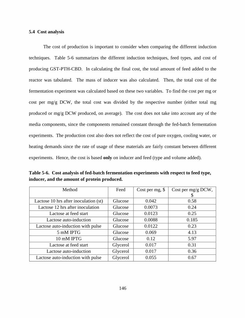
146
5.4 Cost analysis
The cost of production is important to consider when comparing the different induction
techniques. Table 5-6 summarizes the different induction techniques, feed types, and cost of
producing GST-PTH-CBD. In calculating the final cost, the total amount of feed added to the
reactor was tabulated. The mass of inducer was also calculated. Then, the total cost of the
fermentation experiment was calculated based on these two variables. To find the cost per mg or
cost per mg/g DCW, the total cost was divided by the respective number (either total mg
produced or mg/g DCW produced, on average). The cost does not take into account any of the
media components, since the components remained constant through the fed-batch fermentation
experiments. The production cost also does not reflect the cost of pure oxygen, cooling water, or
heating demands since the rate of usage of these materials are fairly constant between different
experiments. Hence, the cost is based only on inducer and feed (type and volume added).
Table 5-6. Cost analysis of fed-batch fermentation experiments with respect to feed type,
inducer, and the amount of protein produced.
Method Feed Cost per mg, $ Cost per mg/g DCW,
$
Lactose 10 hrs after inoculation (st) Glucose 0.042 0.58
Lactose 12 hrs after inoculation Glucose 0.0073 0.24
Lactose at feed start Glucose 0.0123 0.25
Lactose auto-induction Glucose 0.0088 0.185
Lactose auto-induction with pulse Glucose 0.0122 0.23
5 mM IPTG Glucose 0.069 4.13
10 mM IPTG Glucose 0.12 5.97
Lactose at feed start Glycerol 0.017 0.31
Lactose auto-induction Glycerol 0.017 0.36
Lactose auto-induction with pulse Glycerol 0.055 0.67

147
As summarized in Table 5-6, the IPTG-induced cultures cost over ten times the
amount to produce 1 mg protein per g DCW when compared to lactose-induced cultures. In
the case of the IPTG-induced experiments, the cost of IPTG was the driving force. In other
experiments, the amount of feed added to the reactor was what typically drove the cost high.
Glycerol is more expensive to use as a feed source than glucose, but the feeding rates in glycerol-
fed fermentations didn't reach as high of flow rates since the cultivations didn't last as long.
In considering the costs of manufacturing, it is important to compare the numbers with
respect to grams of DCW because this takes into account the total amount of cells produced in
the culture (i.e. the optical density or denseness of the culture). For example, the cost of
production of protein using the saw-tooth feeding profile with lactose induction was high, not
because of the amount of feed or the inducer type, but because the final cell density was high for
the amount of total protein produced. Hence, the cost associated with the fermentation divided
by a low mg/g DCW number leaves a resulting higher cost. On the other hand, the glucose-fed
lactose-induced at 12 hours experiment cost half as much because the cost was divided by a
higher mg/g DCW number. The fermentation with the lowest cost was the auto-induction
glucose-fed experiment. This cultivation had a lower cell density, but a higher amount of protein
was produced. Hence, the value of mg/g DCW was higher.
Since IPTG-induced experiments produced the most protein, but the cost was high, one
can examine how many fermentation experiments would be necessary to complete to duplicate
the amount of protein produced from IPTG using a different induction method. Table 5-7 shows
how many fermentations are required using each method to produced 611 mg protein. This was
the average amount produced from the 10 mM IPTG-induced experiments. Considering the cost
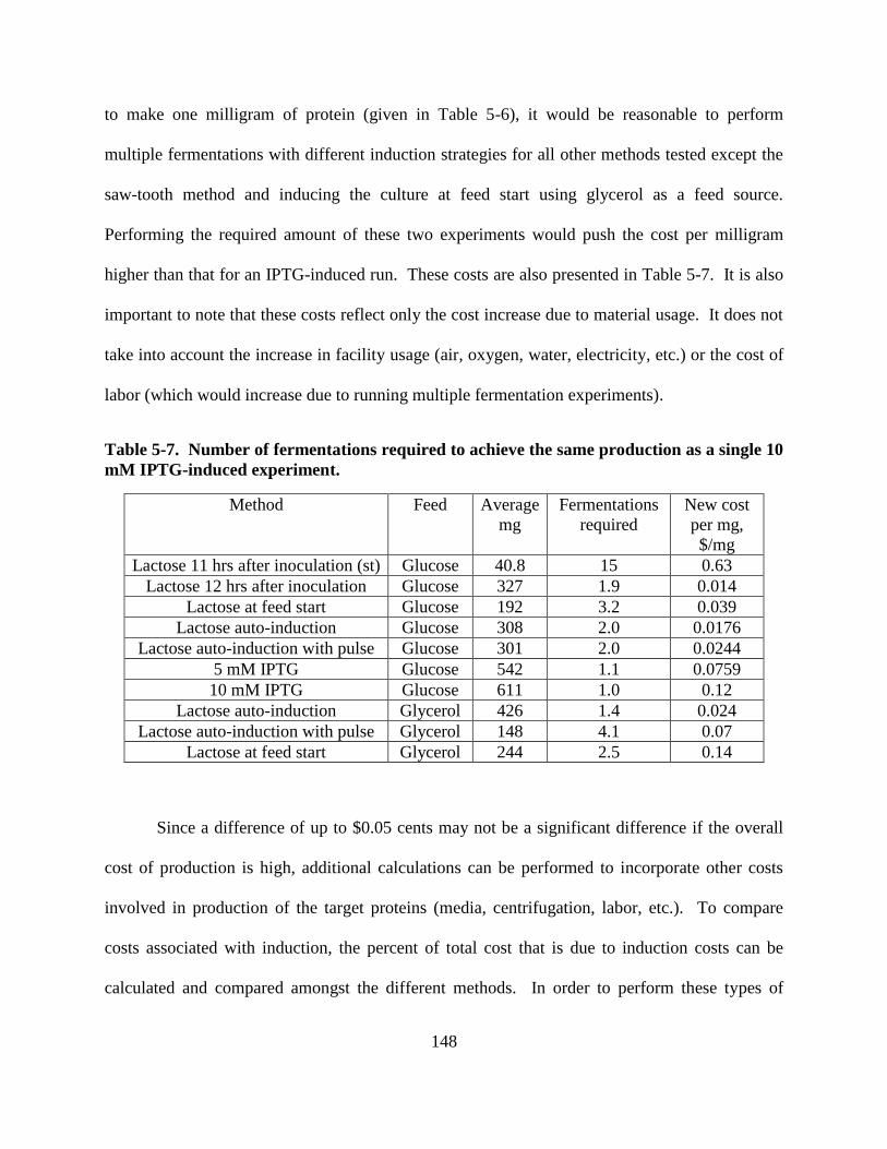
148
to make one milligram of protein (given in Table 5-6), it would be reasonable to perform
multiple fermentations with different induction strategies for all other methods tested except the
saw-tooth method and inducing the culture at feed start using glycerol as a feed source.
Performing the required amount of these two experiments would push the cost per milligram
higher than that for an IPTG-induced run. These costs are also presented in Table 5-7. It is also
important to note that these costs reflect only the cost increase due to material usage. It does not
take into account the increase in facility usage (air, oxygen, water, electricity, etc.) or the cost of
labor (which would increase due to running multiple fermentation experiments).
Table 5-7. Number of fermentations required to achieve the same production as a single 10
mM IPTG-induced experiment.
Method Feed Average
mg
Fermentations
required
New cost
per mg,
$/mg
Lactose 11 hrs after inoculation (st) Glucose 40.8 15 0.63
Lactose 12 hrs after inoculation Glucose 327 1.9 0.014
Lactose at feed start Glucose 192 3.2 0.039
Lactose auto-induction Glucose 308 2.0 0.0176
Lactose auto-induction with pulse Glucose 301 2.0 0.0244
5 mM IPTG Glucose 542 1.1 0.0759
10 mM IPTG Glucose 611 1.0 0.12
Lactose auto-induction Glycerol 426 1.4 0.024
Lactose auto-induction with pulse Glycerol 148 4.1 0.07
Lactose at feed start Glycerol 244 2.5 0.14
Since a difference of up to $0.05 cents may not be a significant difference if the overall
cost of production is high, additional calculations can be performed to incorporate other costs
involved in production of the target proteins (media, centrifugation, labor, etc.). To compare
costs associated with induction, the percent of total cost that is due to induction costs can be
calculated and compared amongst the different methods. In order to perform these types of
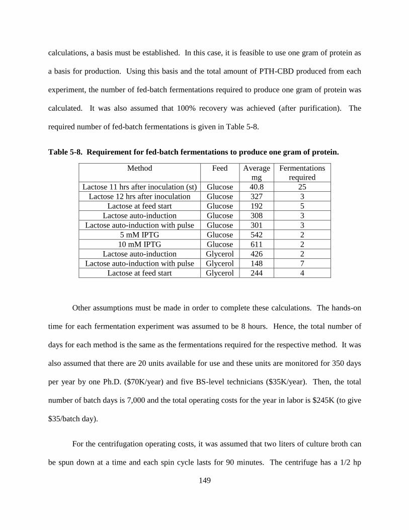
149
calculations, a basis must be established. In this case, it is feasible to use one gram of protein as
a basis for production. Using this basis and the total amount of PTH-CBD produced from each
experiment, the number of fed-batch fermentations required to produce one gram of protein was
calculated. It was also assumed that 100% recovery was achieved (after purification). The
required number of fed-batch fermentations is given in Table 5-8.
Table 5-8. Requirement for fed-batch fermentations to produce one gram of protein.
Method Feed Average
mg
Fermentations
required
Lactose 11 hrs after inoculation (st) Glucose 40.8 25
Lactose 12 hrs after inoculation Glucose 327 3
Lactose at feed start Glucose 192 5
Lactose auto-induction Glucose 308 3
Lactose auto-induction with pulse Glucose 301 3
5 mM IPTG Glucose 542 2
10 mM IPTG Glucose 611 2
Lactose auto-induction Glycerol 426 2
Lactose auto-induction with pulse Glycerol 148 7
Lactose at feed start Glycerol 244 4
Other assumptions must be made in order to complete these calculations. The hands-on
time for each fermentation experiment was assumed to be 8 hours. Hence, the total number of
days for each method is the same as the fermentations required for the respective method. It was
also assumed that there are 20 units available for use and these units are monitored for 350 days
per year by one Ph.D. ($70K/year) and five BS-level technicians ($35K/year). Then, the total
number of batch days is 7,000 and the total operating costs for the year in labor is $245K (to give
$35/batch day).
For the centrifugation operating costs, it was assumed that two liters of culture broth can
be spun down at a time and each spin cycle lasts for 90 minutes. The centrifuge has a 1/2 hp
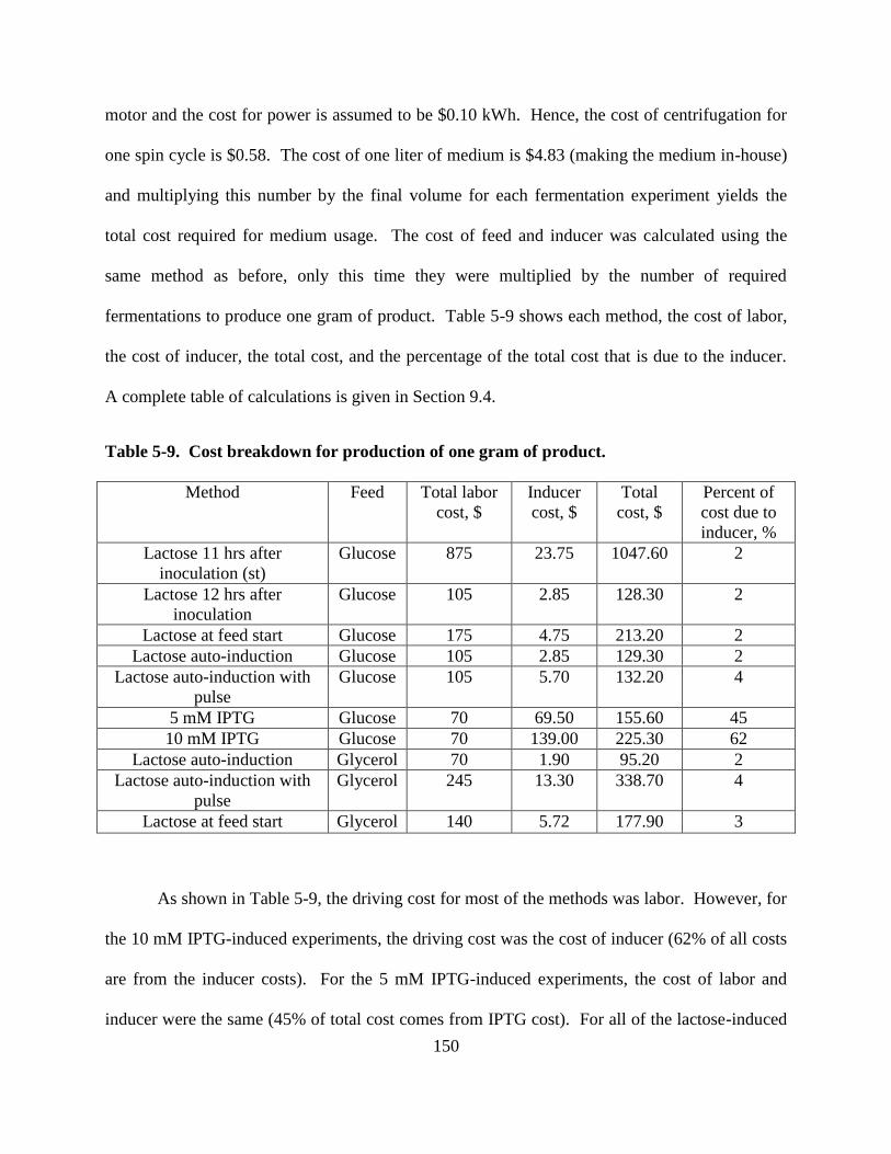
150
motor and the cost for power is assumed to be $0.10 kWh. Hence, the cost of centrifugation for
one spin cycle is $0.58. The cost of one liter of medium is $4.83 (making the medium in-house)
and multiplying this number by the final volume for each fermentation experiment yields the
total cost required for medium usage. The cost of feed and inducer was calculated using the
same method as before, only this time they were multiplied by the number of required
fermentations to produce one gram of product. Table 5-9 shows each method, the cost of labor,
the cost of inducer, the total cost, and the percentage of the total cost that is due to the inducer.
A complete table of calculations is given in Section 9.4.
Table 5-9. Cost breakdown for production of one gram of product.
Method Feed Total labor
cost, $
Inducer
cost, $
Total
cost, $
Percent of
cost due to
inducer, %
Lactose 11 hrs after
inoculation (st)
Glucose 875 23.75 1047.60 2
Lactose 12 hrs after
inoculation
Glucose 105 2.85 128.30 2
Lactose at feed start Glucose 175 4.75 213.20 2
Lactose auto-induction Glucose 105 2.85 129.30 2
Lactose auto-induction with
pulse
Glucose 105 5.70 132.20 4
5 mM IPTG Glucose 70 69.50 155.60 45
10 mM IPTG Glucose 70 139.00 225.30 62
Lactose auto-induction Glycerol 70 1.90 95.20 2
Lactose auto-induction with
pulse
Glycerol 245 13.30 338.70 4
Lactose at feed start Glycerol 140 5.72 177.90 3
As shown in Table 5-9, the driving cost for most of the methods was labor. However, for
the 10 mM IPTG-induced experiments, the driving cost was the cost of inducer (62% of all costs
are from the inducer costs). For the 5 mM IPTG-induced experiments, the cost of labor and
inducer were the same (45% of total cost comes from IPTG cost). For all of the lactose-induced

151
experiments, the percentage of cost due to inducer cost remained below 4%. Additionally, it is
still feasible to perform multiple experiments using alternative induction techniques. All but two
experiments (saw-tooth and lactose auto-induction with pulse and glycerol feed) cost less than
the 10 mM IPTG-induced experiments. These costs reflect only the costs involved with the
fermentation and production portion of the bioprocessing process. Downstream processing costs
were not included in this cost analysis.
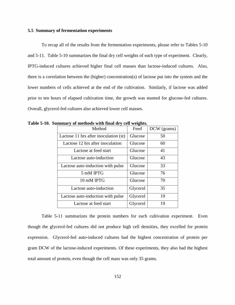
152
5.5 Summary of fermentation experiments
To recap all of the results from the fermentation experiments, please refer to Tables 5-10
and 5-11. Table 5-10 summarizes the final dry cell weights of each type of experiment. Clearly,
IPTG-induced cultures achieved higher final cell masses than lactose-induced cultures. Also,
there is a correlation between the (higher) concentration(s) of lactose put into the system and the
lower numbers of cells achieved at the end of the cultivation. Similarly, if lactose was added
prior to ten hours of elapsed cultivation time, the growth was stunted for glucose-fed cultures.
Overall, glycerol-fed cultures also achieved lower cell masses.
Table 5-10. Summary of methods with final dry cell weights.
Method Feed DCW (grams)
Lactose 11 hrs after inoculation (st) Glucose 50
Lactose 12 hrs after inoculation Glucose 60
Lactose at feed start Glucose 41
Lactose auto-induction Glucose 43
Lactose auto-induction with pulse Glucose 33
5 mM IPTG Glucose 76
10 mM IPTG Glucose 70
Lactose auto-induction Glycerol 35
Lactose auto-induction with pulse Glycerol 19
Lactose at feed start Glycerol 19
Table 5-11 summarizes the protein numbers for each cultivation experiment. Even
though the glycerol-fed cultures did not produce high cell densities, they excelled for protein
expression. Glycerol-fed auto-induced cultures had the highest concentration of protein per
gram DCW of the lactose-induced experiments. Of these experiments, they also had the highest
total amount of protein, even though the cell mass was only 35 grams.
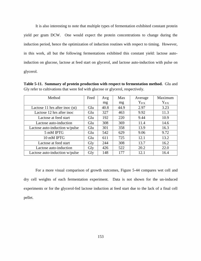
153
It is also interesting to note that multiple types of fermentation exhibited constant protein
yield per gram DCW. One would expect the protein concentrations to change during the
induction period, hence the optimization of induction routines with respect to timing. However,
in this work, all but the following fermentations exhibited this constant yield: lactose auto-
induction on glucose, lactose at feed start on glycerol, and lactose auto-induction with pulse on
glycerol.
Table 5-11. Summary of protein production with respect to fermentation method. Glu and
Gly refer to cultivations that were fed with glucose or glycerol, respectively.
Method Feed Avg
mg
Max
mg
Average
YP/X
Maximum
YP/X
Lactose 11 hrs after inoc (st) Glu 40.8 44.9 2.97 3.23
Lactose 12 hrs after inoc Glu 327 463 9.92 11.3
Lactose at feed start Glu 192 220 9.44 10.9
Lactose auto-induction Glu 308 369 11.4 14.6
Lactose auto-induction w/pulse Glu 301 358 13.9 16.3
5 mM IPTG Glu 542 629 9.06 9.72
10 mM IPTG Glu 611 725 12.1 13.2
Lactose at feed start Gly 244 308 13.7 16.2
Lactose auto-induction Gly 426 522 20.2 22.0
Lactose auto-induction w/pulse Gly 148 177 12.1 16.4
For a more visual comparison of growth outcomes, Figure 5-44 compares wet cell and
dry cell weights of each fermentation experiment. Data is not shown for the un-induced
experiments or for the glycerol-fed lactose induction at feed start due to the lack of a final cell
pellet.
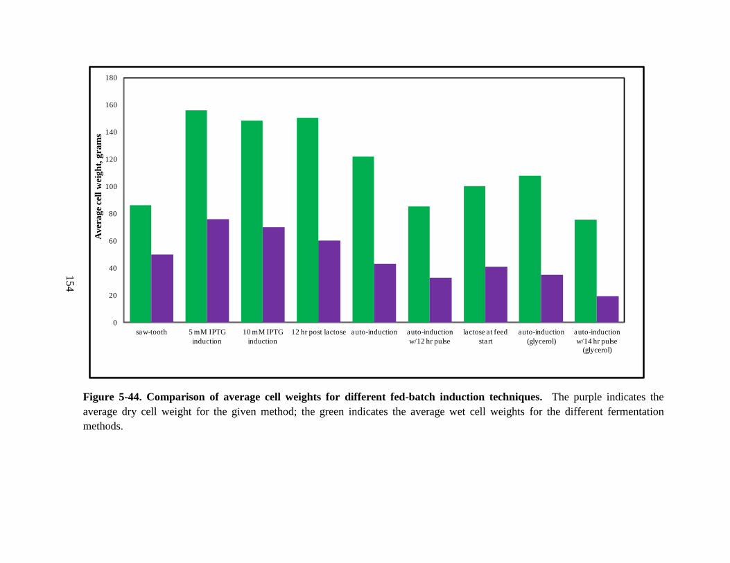
Figure 5-44. Comparison of average cell weights for different fed-batch induction techniques. The purple indicates the
average dry cell weight for the given method; the green indicates the average wet cell weights for the different fermentation
methods.
0
20
40
60
80
100
120
140
160
180
saw-tooth 5 mM IPTG
induction
10 mM IPTG
induction
12 hr post lactose auto-induction auto-induction
w/12 hr pulse
lactose at feed
start
auto-induction
(glycerol)
auto-induction
w/14 hr pulse
(glycerol)
Av
era
ge
cell
wei
gh
t, g
ram
s
154

155
The analysis of carbohydrates led to some interesting insights into the fermentation
system. First of all, glucose accumulation was much more extensive in induced experiments.
Recall that for the un-induced experiments glucose accumulation did not occur until the very end
of the fermentation experiment (24 hours after inoculation). For induced experiments, glucose
accumulation began around 12 hours after inoculation in some cases. This shows that induction
(protein expression) has a substantial effect on the uptake of glucose but not necessarily on the
growth of the culture (in the IPTG-induced experiments). Also, in the case of the IPTG-induced
experiments, glucose accumulated at higher amounts even though the growth for these cultures
was better than those induced with lactose. For lactose-induced cultures, this indicates that less
glucose must not be used only for increasing biomass and is used elsewhere in the system.
Hence, lactose has an effect on how glucose is used, but not how glucose is taken up by the cells.
If lactose was affecting glucose uptake rates, one would expect to witness higher concentrations
of glucose in the supernatants. This was not the case. Additionally, the earlier on that lactose
was introduced into the system, the lower the final dry cell weight of the culture was. For
example, the results from the experiment in which lactose was introduced into the fermentation
12 hours after inoculation were similar to those from IPTG-induced experiments with respect to
glucose accumulation and growth. When lactose was added when feed started, growth was
similar to auto-induced cultures.
In an attempt to better describe the observation that lactose induction negatively affects
cell growth when it is added earlier on during the fermentation experiment, the yield of biomass
from glucose was calculated by plotting the total biomass versus the amount of feed consumed.
Table 5-12 summarizes the results from these calculations. From the literature, it was expected
that the yields from glycerol would be lower than the yields from glucose. Garcia-Arrazola et al.
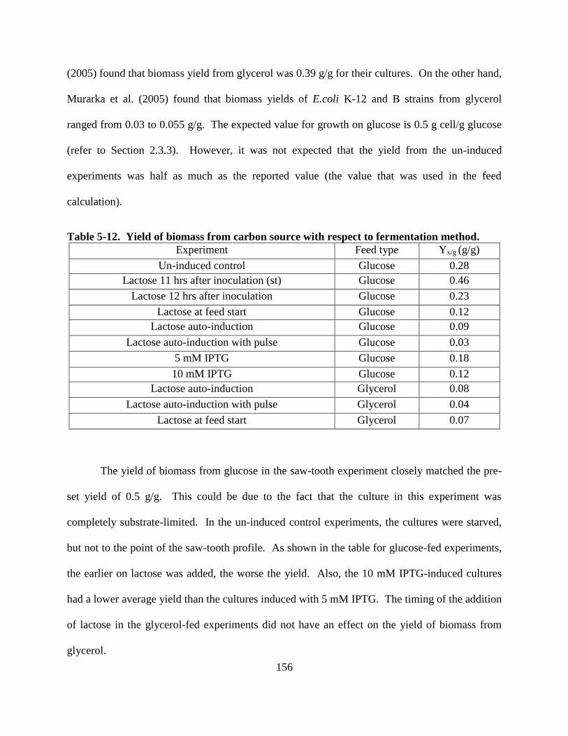
156
(2005) found that biomass yield from glycerol was 0.39 g/g for their cultures. On the other hand,
Murarka et al. (2005) found that biomass yields of E.coli K-12 and B strains from glycerol
ranged from 0.03 to 0.055 g/g. The expected value for growth on glucose is 0.5 g cell/g glucose
(refer to Section 2.3.3). However, it was not expected that the yield from the un-induced
experiments was half as much as the reported value (the value that was used in the feed
calculation).
Table 5-12. Yield of biomass from carbon source with respect to fermentation method.
Experiment Feed type Yx/g (g/g)
Un-induced control Glucose 0.28
Lactose 11 hrs after inoculation (st) Glucose 0.46
Lactose 12 hrs after inoculation Glucose 0.23
Lactose at feed start Glucose 0.12
Lactose auto-induction Glucose 0.09
Lactose auto-induction with pulse Glucose 0.03
5 mM IPTG Glucose 0.18
10 mM IPTG Glucose 0.12
Lactose auto-induction Glycerol 0.08
Lactose auto-induction with pulse Glycerol 0.04
Lactose at feed start Glycerol 0.07
The yield of biomass from glucose in the saw-tooth experiment closely matched the pre-
set yield of 0.5 g/g. This could be due to the fact that the culture in this experiment was
completely substrate-limited. In the un-induced control experiments, the cultures were starved,
but not to the point of the saw-tooth profile. As shown in the table for glucose-fed experiments,
the earlier on lactose was added, the worse the yield. Also, the 10 mM IPTG-induced cultures
had a lower average yield than the cultures induced with 5 mM IPTG. The timing of the addition
of lactose in the glycerol-fed experiments did not have an effect on the yield of biomass from
glycerol.

157
Prior to fed-batch fermentation experiments, it was thought that acetic acid would be
inhibitory to growth due to the accumulation of the substrate in the media. As previously
discussed, this is often an issue in fed-batch fermentations. However, under conditions where
glucose accumulation occurred, acetic acid accumulation remained low. This characteristic of
the different fermentations tested may mirror that that was witnessed by Shiloach et al. (1996) -
BL21 does a decent job of self-regulating acetic acid accumulation by re-consuming the
substrate. This phenomenon has been witnessed by others as well. Varma and Palsson (1994b)
report on acetate re-consumption in the presence of glucose feed. They propose that high cell
densities can result in the consumption of glucose and acetate simultaneously. This would
account for the leveling-off of acetic acid concentration in the supernatant in many of the
fermentation experiments. At some point during cultivation, the TCA cycle may become
saturated due to the metabolism of glucose. After saturation, the amount of acetate produced
(per cell) becomes steady. Due to the increase in the number of cells, one would expect that the
acetate concentration in the system would increase. However, this was not seen, so perhaps
BL21 does regulate acetate concentrations.
Recall that the glycerol feed contained the same molar concentrations of carbon as the
glucose feed. In glycerol-fed experiments, the concentration of glycerol at the end of the
experiment was extremely high. Even though the molar carbon content was the same, glycerol
uptake was much slower, which resulted in lower dry cell weights and high concentrations of
extracellular glycerol. It was expected that the slower uptake of glycerol would result in the
inhibition of acetic acid production. This was also not the case, but glycerol feed was not
utilized due to its ability to decrease the production of acetate. The production of acetate from
glycerol was comparable to glucose-fed experiments and never exceeded 2 g/l.
158
As expected (due to the lift on catabolite repression), glycerol did have an effect on the
uptake and consumption of lactose. For auto-induced cultures, lactose was absent at 15 hours
after inoculation for the glycerol-fed culture. For the glucose-fed cultures, lactose was still
present. Similarly, lactose was absent in the samples after 20 hours from the auto-induced
cultures with a pulse and glycerol feed. In glucose-fed experiments, 4 g/l lactose still remained
after 22 hours of cultivation. In all of the glycerol-fed experiments, lactose was depleted prior to
the end of cultivation. This was not the case for the glucose-fed experiments.
5.6 Fine analysis of product
Remember from Section 5-1 that there was a significant amount of GST that was present
as a degraded protein or truncated product in the cell lysate. This product ran at approximately
26 kDa on a SDS-PAGE gel (refer to Figure 5-8). From its reaction with the anti-bodies specific
for GST, its appearance in the eluted portion of the product obtained from purification
experiments, and mass spectrometry (MS) analysis, this product was confirmed as being GST.
However, this product does not exist in this concentration in the fed-batch fermentation
experiments. A similar band appeared at the same molecular weight, but this band was absent on
the western blots performed. After this observation, the band was sent in for sequencing. The
sequencing results revealed that the intense band at 26 kDa was β-lactamase. Figure 5-45 shows
a gel that was used for densitometry with an intense band representing β-lactamase. The MS
data indicates that of 47 tryptic fragments of GST, only one peak appears on the spectrum.
β-lactamase is present in gram-negative bacteria and accounts for its antibiotic resistance.
It can hydrolyze ampicillin and related drugs by breaking apart the beta-lactam ring (Jacoby and
Sutton, 1985). The concentration of β-lactamase in the lysates of samples from fed-batch

159
cultures remains steady throughout the fermentation. The expression of β-lactamase is typically
constitutive - or continually expressed. It would be expected that this concentration would
decrease due to both the breakdown of ampicillin during the process and to the increasing
volume of the reactor. The increase in volume would assure that the cells come in contact with
less antibiotic. However, if cells are under a stressed environment, expression of this protein
may occur. Cultures in fed-batch fermentation may suffer from some of the stresses reported in
Section 2.3. These stresses can influence changes in plasmid production, which in turn could
cause over-expression of β-lactamase.
Additionally, it was reported that increased metabolic burden (from gene expression) can
cause runaway plasmid replication (Camps, 2010). If so, then this would account for the
increase in β-lactamase expression. However, one would also expect to see higher
concentrations of product, as long as inducer is still present in the system. Since the same results
were found for IPTG and lactose-induced systems, this must not be the case because IPTG
cannot be metabolized by the cells.
Figure 5-45. Sample SDS-PAGE gel showing β-lactamase.
GST-PTH-CBD
Β-lactamase
50 kDa
25 kDa

160
According to Hong et al. (1992), using glycerol at a concentration of 50 g/l caused a 5-
fold increase in recombinant β-lactamase in flask cultures. They do not see this increase without
IPTG or with growth on glucose. While this is interesting and could be a cause for production
on glycerol, this strong band is also seen in lysates from cells grown on glucose and in the
absence of IPTG. Thus, glycerol feed must not be the cause for the appearance of a strong β-
lactamase band.
5.7 Purification, activity analysis, and cleavage
Select lysates were purified using affinity purification techniques. A sample of a SDS-
PAGE gel after purification is shown in Figure 5-46. Most of the product eluted in two aliquots
(of 1 ml each). This occurred after two to three milliliters of elution buffer passed through the
column (reference Figure 2-5 for the chromatogram). Also, the gel did not indicate that there
was degraded GST in the lysate as the lower band representative of GST is absent. However, the
western blot in Figure 5-47 showed these degraded bands.
From the following two figures, one can conclude that affinity chromatography with a
GST-tag was a viable option for purification of the product.

161
Figure 5-46. SDS-PAGE shows purity of fractions. Lane 1 - molecular weight marker; Lane
2 - lysate loaded to the column; Lane 3 - flow through: Lane 4 and 5- eluted fractions.
Figure 5-47. Western blot after purification shows some degraded product. This western
blot correlates with the gel in Figure 5-46. Lane 1 - ladder marker; Lane 2 - lysate added to
column; Lane 3 - flow through; Lanes indicated by 4 - eluted samples.
50 kDa
25
37
GST-PTH-CBD
1 2 3 4 5
50 kDa
37
25
1 2 3 4
GST-PTH-CBD
GST

162
To check the collagen-binding activity of the collagen-binding domain, purified GST-
PTH-CBD was incubated with collagen sheets. Equal amounts of green fluorescent protein and
GST-PTH-CBD were incubated for a specified amount of time. As shown in Figure 5-48, the
collagen sheet incubated with GST-PTH-CBD reacted with the visualization solution used in the
western blotting protocol. This indicated that GST-PTH-CBD retained its collagen-binding
activity and bound to the collagen sheet. On the other hand, little to no reaction occurred in the
control samples. The slight coloration in these samples was due to the sensitivity of the
visualization solution to light.
Figure 5-48. Activity analysis for GST-PTH-CBD using collagen binding sheets. There was
an intense signal for GST-PTH-CBD on the collagen sheet, as indicated by the image on the far
right.
In order to check cleavage of the tag, purified lysate was incubated overnight with Factor
Xa. Cleavage must be performed prior to any testing of the activity of parathyroid hormone or

163
use of the target product. As shown in Figure 5-49, cleavage occurred. After incubation, the
sample contained no 44 kDa protein, as indicated by the disappearance of the band that is in
lanes 2 and 3. There was also the appearance of a very weak band at approximately 18 kDa with
a band at approximately 20 kDa. The PTH-CBD portion of the protein runs between these two
molecular weights. This region is indicated by the oval on the gel in Figure 5-49.
Figure 5-49. SDS-PAGE gel indicates cleavage of the GST tag using Factor Xa. Factor Xa
shows up as two bands on reducing gel - 34 and 29 kDa. Lane 1 - Ladder marker; Lane 2 -
purified lysate; Lane 3 - initial sample of purified lysate with Factor Xa (0 hr); Lane 4 - lysate
after incubation with Factor Xa.
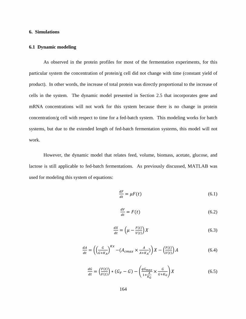
164
6. Simulations
6.1 Dynamic modeling
As observed in the protein profiles for most of the fermentation experiments, for this
particular system the concentration of protein/g cell did not change with time (constant yield of
product). In other words, the increase of total protein was directly proportional to the increase of
cells in the system. The dynamic model presented in Section 2.5 that incorporates gene and
mRNA concentrations will not work for this system because there is no change in protein
concentration/g cell with respect to time for a fed-batch system. This modeling works for batch
systems, but due to the extended length of fed-batch fermentation systems, this model will not
work.
However, the dynamic model that relates feed, volume, biomass, acetate, glucose, and
lactose is still applicable to fed-batch fermentations. As previously discussed, MATLAB was
used for modeling this system of equations:
(6.1)
(6.2)
(6.3)
(6.4)
(6.5)
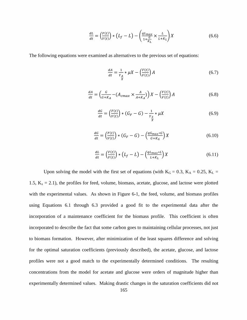
165
(6.6)
The following equations were examined as alternatives to the previous set of equations:
(6.7)
(6.8)
(6.9)
(6.10)
(6.11)
Upon solving the model with the first set of equations (with KG = 0.3, KA = 0.25, KL =
1.5, Kx = 2.1), the profiles for feed, volume, biomass, acetate, glucose, and lactose were plotted
with the experimental values. As shown in Figure 6-1, the feed, volume, and biomass profiles
using Equations 6.1 through 6.3 provided a good fit to the experimental data after the
incorporation of a maintenance coefficient for the biomass profile. This coefficient is often
incorporated to describe the fact that some carbon goes to maintaining cellular processes, not just
to biomass formation. However, after minimization of the least squares difference and solving
for the optimal saturation coefficients (previously described), the acetate, glucose, and lactose
profiles were not a good match to the experimentally determined conditions. The resulting
concentrations from the model for acetate and glucose were orders of magnitude higher than
experimentally determined values. Making drastic changes in the saturation coefficients did not
166
affect the difference between the simulated values and the experimental values. While the final
simulated values for lactose concentrations were a decent fit numerically, the slope for the
consumption of lactose did not match that from the actual experiment. According to the model,
as soon as lactose entered the system it began being consumed. Experimentally, as seen with
diauxic growth, there is a lag phase after glucose is consumed for the cells to adjust to a
secondary carbohydrate source. This model indicates that lactose was preferentially consumed
over glucose, with no lag phase. As shown in Figure 6-1, glucose accumulated to values over
300 g/l, but lactose consumption began immediately after its introduction to the system.***
(a)
***
For the remaining figures for the dynamic models, the open circles are representative of the
experimental data points. The solid line is the simulated profile. Lastly, the arrows indicate the
direction of the increase in the saturation coefficients, where applicable.
Time, hours
feed
ra
te,
l/h
; v
olu
me,
l
167
(b)
Time, hours
Bio
mass
, g;
glu
cose
, g/l;
ace
tate
, g/l
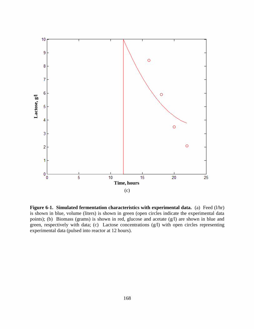
168
(c)
Figure 6-1. Simulated fermentation characteristics with experimental data. (a) Feed (l/hr)
is shown in blue, volume (liters) is shown in green (open circles indicate the experimental data
points); (b) Biomass (grams) is shown in red, glucose and acetate (g/l) are shown in blue and
green, respectively with data; (c) Lactose concentrations (g/l) with open circles representing
experimental data (pulsed into reactor at 12 hours).
Time, hours
Lact
ose
, g/l

169
It is clear that feed, volume, and biomass can be successfully simulated by manipulating
the maintenance coefficient (depending on the experiment that is being simulated), but further
examination of acetate, glucose, and lactose is required. To check this model with other types of
fermentation experiments, the experimental data for the 5 mM IPTG-induced cultures was
compared with the simulated values (for acetate and glucose). After fitting the feed, volume, and
biomass, and after optimization of the saturation coefficients, the carbohydrate profiles were still
orders of magnitude higher than the experimental values. Hence, the model did not properly
convey the relationship between glucose, acetate, and lactose.
In an attempt to find a simulation that better describes the relationships between the
carbohydrates, different combinations of equations were simulated where Equations 6.7 and 6.8
replaced Equation 6.4, Equations 6.9 and 6.10 replaced Equation 6.5, and Equation 6.11 replaced
Equation 6.6. This resulted in 18 different permutations of the model where the equations for
feed, volume, and biomass remained the same.
The first simulation tested the alternative lactose equation (Equation 6.11 for Equation
6.6). Figure 6-2 shows the profiles for acetate, glucose, and lactose after incorporation of the
alternative equation.

170
Figure 6-2. Simulation using alternative lactose equation. Lactose profile is shown in red;
glucose profile is shown in green, and acetate profile is shown in blue. The sharp increase at 12
hours indicates that lactose has been added to the reactor.
This substitution did not aid in the fitting of lactose to experimental values. After 15
hours, lactose sharply declined while glucose steadily increased. Optimizing the saturation
coefficient for lactose did not change the rate at which lactose was consumed. Hence, the model
did not sufficiently describe the catabolite repression relationship that exists between glucose and
lactose. One would not expect to see a decline in lactose concentration immediately after adding
it to the system if glucose has accumulated to concentrations exceeding 100 g/l.
Simulations containing Equation 6.7 instead of Equation 6.4 resulted in acetate
concentrations between 3000 and 6000 g/l depending on the optimized KA value and the
accompanying glucose equation. As a result, it was determined that Equation 6.7 would not be

171
sufficient at modeling the acetate profiles for the set of experiments performed for this
dissertation. This observation was interesting because Equation 6.7 was so widely accepted in
the literature (Mohseni et al., 2009; Roeva et al., 2007). However, the models used in the
literature did not incorporate the addition of lactose to the system. Simulations containing 6.8
instead of 6.4 yielded no apparent difference in the projected acetate profiles after optimization
of the saturation coefficients from the original model (the equations are the same if Kx = 1).
Since the modeling of acetate was unsuccessful and since acetate concentrations
remained less than 2g/l for the majority of the experiments, the next simulations focused on
modeling only glucose and lactose. Four different permutations of the simulation were tested
with no acetate equation in the model (Equation 6.10 is equivalent to Equation 6.5 with no
acetate, so there were only four permutations instead of six). The first of these permutations
tested the original equations for glucose and lactose. The resultant profiles from this model are
shown in Figure 6-3. Figure 6-3 (a) shows the results from examining the effect of changing the
saturation coefficient for glucose only. Increasing KG caused an increase in the rate at which
glucose accumulated. Inversely, decreasing KG caused an increase in glucose consumption
during the batch phase of the fermentation. With this model (with no acetate equation), the
overall glucose concentrations decreased so that they were no longer orders of magnitude higher
than those that were experimentally determined. Figure 6-3 (b) shows the change in profiles
with respect to changing the saturation coefficient of lactose. Changing KL resulted in a change
in the rate at which lactose is consumed. The general slope of the simulated lactose profile
matched the slope of the consumption of lactose from experimentally determined data, and this
slope is a better “fit” as the coefficient increases. Graph (c) of Figure 6-3 shows the profiles with
optimized saturation coefficients. For these profiles, the glucose and lactose saturation
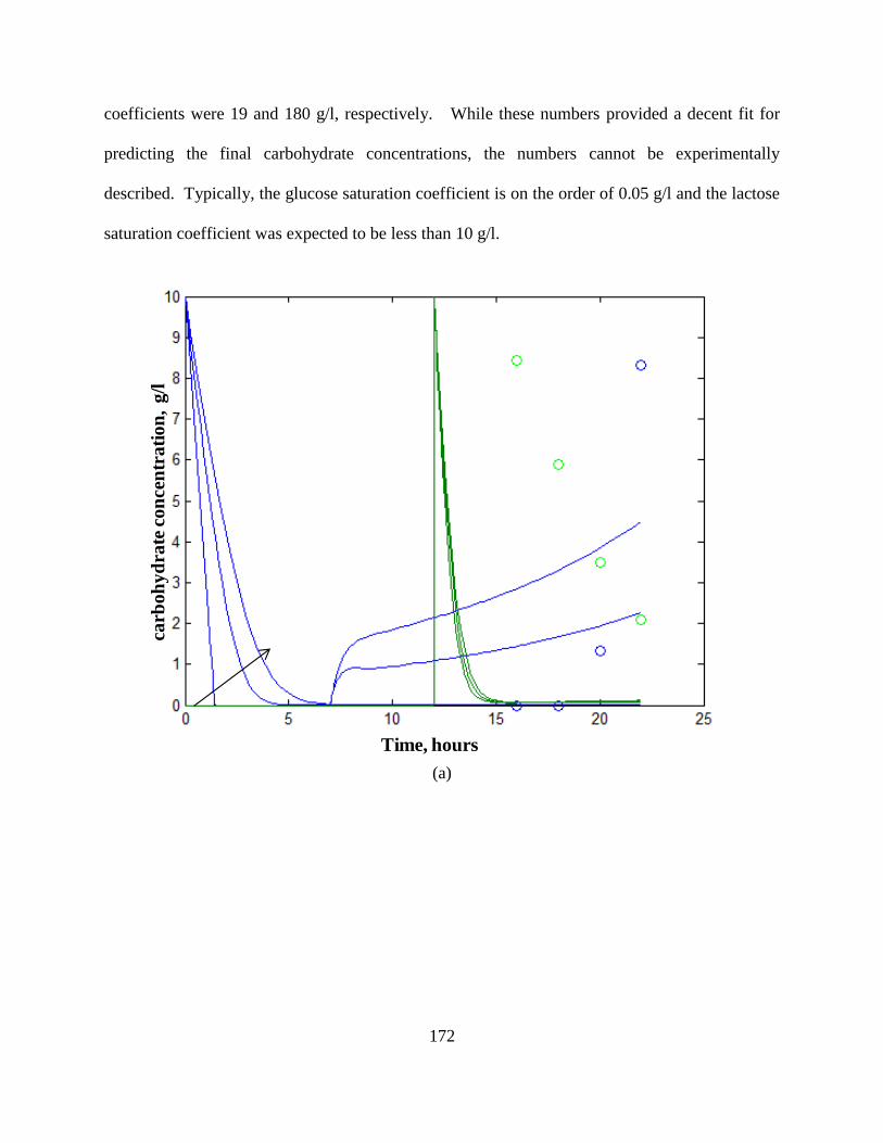
172
coefficients were 19 and 180 g/l, respectively. While these numbers provided a decent fit for
predicting the final carbohydrate concentrations, the numbers cannot be experimentally
described. Typically, the glucose saturation coefficient is on the order of 0.05 g/l and the lactose
saturation coefficient was expected to be less than 10 g/l.
(a)
Time, hours
carb
oh
yd
rate
con
cen
trati
on
, g/l

173
(b)
(c)
Figure 6-3. Simulation using original glucose and lactose equations without acetate
equation. Lactose is given in green, glucose is given in blue. (a) Increase in glucose coefficient
causes increase in final glucose numbers (KG = 0.05, 1, 5); (b) Increase in saturation coefficient
of lactose increases final simulated lactose values (KL = 10, 50, 100, and 150); (c) “Optimized”
saturation coefficients show match in final carbohydrate concentrations (KG = 19 g/l, KL = 180
g/l).
carb
oh
yd
rate
co
nce
ntr
ati
on
, g
/l
Time, hours
Time, hours
Carb
oh
yd
rate
con
cen
trati
on
, g/l
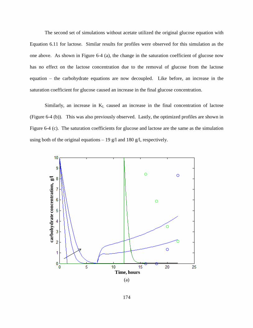
174
The second set of simulations without acetate utilized the original glucose equation with
Equation 6.11 for lactose. Similar results for profiles were observed for this simulation as the
one above. As shown in Figure 6-4 (a), the change in the saturation coefficient of glucose now
has no effect on the lactose concentration due to the removal of glucose from the lactose
equation – the carbohydrate equations are now decoupled. Like before, an increase in the
saturation coefficient for glucose caused an increase in the final glucose concentration.
Similarly, an increase in KL caused an increase in the final concentration of lactose
(Figure 6-4 (b)). This was also previously observed. Lastly, the optimized profiles are shown in
Figure 6-4 (c). The saturation coefficients for glucose and lactose are the same as the simulation
using both of the original equations – 19 g/l and 180 g/l, respectively.
(a)
carb
oh
yd
rate
co
nce
ntr
ati
on
, g
/l
Time, hours

175
(b)
(c)
Figure 6-4. Simulation with original glucose equation and alternative lactose equation
(without acetate). Lactose is given in green, glucose is given in blue. (a) Increase in glucose
coefficient causes increase in final glucose numbers (KG = 0.05, 1, 5); (b) Increase in saturation
coefficient of lactose increases final simulated lactose values (KL = 10, 50, 100, and 150); (c)
“Optimized” saturation coefficients show match in final carbohydrate concentrations (KG = 19
g/l, KL = 180 g/l). Experimental data points are represented by the open circles.
carb
oh
yd
rate
co
nce
ntr
ati
on
, g
/l
Time, hours
Carb
oh
yd
rate
con
cen
trati
on
, g/l
Time, hours

176
After comparing the profiles in Figures 6-3 and 6-4, it is apparent that there was no
significant difference between using the original lactose equation and the alterative equation
(Equation 6.11) with the original glucose equation. The decoupling of the carbohydrates had
little effect on the overall system. The next set of simulations examined the use of the alternative
glucose equation (Equation 6.9).
Figure 6-5. Simulation of alternative glucose and original lactose equations. Lactose is
given in green; glucose is represented by blue.
As shown in Figure 6-5, the alternative glucose equation (Equation 6.9) coupled with the
original lactose equation (Equation 6.6) was a worse fit for the representation of the experimental
data. Since Equation 6.9 is used, unlike before, there were no parameters that could be changed
to try to modify the profile. The lactose profile was still a decent fit for the experimental data
and like before, increasing the coefficient for lactose caused an increase in the final lactose
carb
oh
yd
rate
co
nce
ntr
ati
on
, g
/l
Time, hours
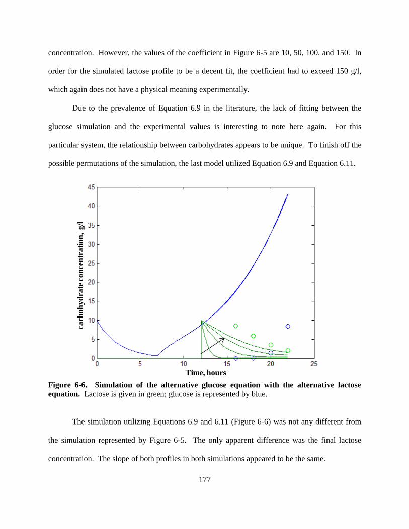
177
concentration. However, the values of the coefficient in Figure 6-5 are 10, 50, 100, and 150. In
order for the simulated lactose profile to be a decent fit, the coefficient had to exceed 150 g/l,
which again does not have a physical meaning experimentally.
Due to the prevalence of Equation 6.9 in the literature, the lack of fitting between the
glucose simulation and the experimental values is interesting to note here again. For this
particular system, the relationship between carbohydrates appears to be unique. To finish off the
possible permutations of the simulation, the last model utilized Equation 6.9 and Equation 6.11.
Figure 6-6. Simulation of the alternative glucose equation with the alternative lactose
equation. Lactose is given in green; glucose is represented by blue.
The simulation utilizing Equations 6.9 and 6.11 (Figure 6-6) was not any different from
the simulation represented by Figure 6-5. The only apparent difference was the final lactose
concentration. The slope of both profiles in both simulations appeared to be the same.
carb
oh
yd
rate
con
cen
trati
on
, g/l
Time, hours
178
The simulations using Equation 6.11 instead of Equation 6.6 maintained similar lactose
profiles as before (with each type of equation), but glucose concentrations were high for
simulations utilizing Equation 6.9 instead of Equation 6.5. Since Equation 6.9 takes into
account only the constant consumption of glucose by cells, there were no parameters to change
to try to achieve a better fit. Thus, the alternative glucose equation (prevalent in the literature)
should not be considered for modeling the relationship between the carbohydrates within the
context of this work (Mohseni et al., 2009; Roeva et al., 2007).
Although there is no apparent difference between the lactose equations when
disregarding the presence of acetate, the original lactose equation (Equation 6.6) provided a
better fit when simulations included the acetate equation (refer to Figures 6-1 and 6-2).
Overall, there is not enough information (taken from experiments or from the literature)
to properly describe the relationship between the carbohydrates in the fed-batch fermentation
systems that were examined. Recall that lactose affected the biomass production but not the
glucose uptake rate. This observation is important in that the mass balance of carbon does not
follow results that are typically found for fed-batch fermentation experiments. Apparently, the
introduction of a third carbohydrate (lactose) interrupts the movement of carbon away from
biomass production. The tracking of carbon may aid in filling the gaps for the dynamic
modeling. This was performed using techniques consistent with metabolic flux analysis.
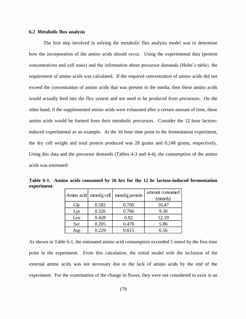
179
6.2 Metabolic flux analysis
The first step involved in solving the metabolic flux analysis model was to determine
how the incorporation of the amino acids should occur. Using the experimental data (protein
concentrations and cell mass) and the information about precursor demands (Holm’s table), the
requirement of amino acids was calculated. If the required concentration of amino acids did not
exceed the concentration of amino acids that was present in the media, then these amino acids
would actually feed into the flux system and not need to be produced from precursors. On the
other hand, if the supplemented amino acids were exhausted after a certain amount of time, these
amino acids would be formed from their metabolic precursors. Consider the 12 hour lactose-
induced experimental as an example. At the 16 hour time point in the fermentation experiment,
the dry cell weight and total protein produced was 28 grams and 0.248 grams, respectively.
Using this data and the precursor demands (Tables 4-3 and 4-4), the consumption of the amino
acids was estimated:
Table 6-1. Amino acids consumed by 16 hrs for the 12 hr lactose-induced fermentation
experiment.
As shown in Table 6-1, the estimated amino acid consumption exceeded 5 mmol by the first time
point in the experiment. From this calculation, the initial model with the inclusion of the
external amino acids was not necessary due to the lack of amino acids by the end of the
experiment. For the examination of the change in fluxes, they were not considered to exist in an
Gly 0.582 0.706 16.47
Lys 0.326 0.706 9.30
Leu 0.428 0.82 12.19
Ser 0.205 0.478 5.86
Asp 0.229 0.615 6.56
amount consumed
(mmols)mmol/g cellAmino acid mmol/g protein
180
external form (outside the cell in the media) and all amino acids for the metabolic flux analysis
must be synthesized. They were not supplied from the culture broth at the fermentation times
that were under investigation.
The data from the glucose-fed experiment with lactose induction at 12 hours was
considered for the first simulation (this fermentation produced the highest biomass of all of the
glucose-fed and lactose-induced experiments). The fluxes (shown in Figure 6-7) were
normalized to the uptake of glucose (r32). Notice that upon normalization, the fluxes throughout
the HMP pathway are high compared to the fluxes of carbon throughout the rest of the pathways
examined. However, the rate of uptake of glucose is similar to the fluxes of carbon throughout
the TCA cycle. Using the final concentrations to take a snap shot of the system using lactose
induction at 12 hours with glucose feed pushed the carbon through the HMP pathway according
to the metabolic flux analysis of the system. Additionally, using the final experimental
concentrations do not allow for the intermediate concentrations to be zero (the sum of the fluxes
at each intermediate component should be zero) after optimization. Also, the optimized biomass
components are low compared to the intermediate fluxes using the final biomass concentration.

181
Figure 6-7. Simulated fluxes from 12 hour lactose-induced cultures with glucose feed.
Amino acids
Cell envelope
Cys, Nucleic acids, Lipids
Ribulose5P
Amino acids
Nucleic acids
Cell Wall
Lipids
Glucoseinternal
Glucose6P
Fructose6P
Glyceraldehyde3P
3PG PEP
Ribose5P
Xylulose5P
Erythrose4P
Amino acids
Ala, Ile, Val
Peptidoglycan
Citrate
α-Ketogluterate
Oxaloacetate
Amino acids
Nucleic acids
Lipids
Acetate
Pyruvate
Acetyl-CoA
21.6
16.7
0.193.8
38.3
14.9
31.727.2 0.8
0.3826.0
0.12
14.3
0.06
12.31.4 0.76
2.71.0
4.6 2.7
1.0
1.0
1.0
0
1.04
0.71
Lactose
26.37
Isocitrate
9.3
0
Glucoseexternal (from feed)0.02
1.0
14.6
Asn, Ile, Met, Thr
Nucleic acids
0.33Lysine
Leucine
Glycine
0.21
0.85
Serine
1.75
Leucine0.42
Lysine
0.33
Aspartate
0.24
Succinate
Malate
0.02
11.4
0.54
= NAD(P)H produced
= FADH produced
= ATP produced
= ATP consumed

182
In order to examine the fluxes for an experiment where the final biomass was lower but
lactose, glucose, and acetate were still present in the system, the auto-induced culture with an
additional lactose pulse was examined. Since all of the carbons were present at the end of the
fermentation, the equations remained the same as those in the simulation for the 12 hour lactose-
induced cultures. The major difference between these two simulations is the final dry cell
weight.
Figure 6-8. Simulated fluxes from auto-induced cultures with an additional pulse of
lactose.
Amino acids
Cell envelope
Cys, Nucleic acids, Lipids
Ribulose5P
Amino acids
Nucleic acids
Cell Wall
Lipids
Glucoseinternal
Glucose6P
Fructose6P
Glyceraldehyde3P
3PG PEP
Ribose5P
Xylulose5P
Erythrose4P
Amino acids
Ala, Ile, Val
Peptidoglycan
Citrate
α-Ketogluterate
Oxaloacetate
Amino acids
Nucleic acids
Lipids
Acetate
Pyruvate
Acetyl-CoA
51.5
41.4
0.459.3
92.4
35.9
76.765.7 2.0
0.9362.9
0.28
34.4
0.15
29.53.33 1.83
6.51.0
11.3 6.48
2.4
2.4
2.4
0.0
2.5
1.97
Lactose
63.8
Isocitrate
22.2
0.0
Glucoseexternal (from feed)0.61
1.0
35.5
Asn, Ile, Met, Thr
Nucleic acids
0.79Lysine
Leucine
Glycine
0.51
2.04
Serine
4.21
Leucine1.02
Lysine
0.79
Aspartate
0.58
Succinate
Malate
0.61
27.8
1.30
= NAD(P)H produced
= FADH produced
= ATP produced
= ATP consumed

183
Compared to the fluxes for the 12 hour lactose-induced experiment, the biomass
component fluxes are higher for this experiment. However, this is due to the fact that the uptake
of glucose was significantly lower. Because of this, comparison of the fluxes between different
experiments does not yield any information about the effects of the differences in biomass
concentrations on metabolism. However, the non-normalized fluxes can be compared. Table 6-
2 gives all of the fluxes for each experiment that was performed utilizing glucose feed. The
glucose uptake rates can be compared, in addition to the fluxes used for synthesis of biomass
components. It is important to note that these fluxes were calculated based on the final
concentrations of carbons and biomass, so the resultant fluxes gave a final snapshot of the system
as a whole. Also, the asterisked fluxes are the fluxes that were used in the optimization routine.
As previously discussed, these fluxes contribute to the precursors for cell wall, amino acid, and
nucleic acid synthesis.

184
Table 6-2. Simulated fluxes for each experiment with glucose feed. Each flux was
normalized to the glucose uptake rate (r32). The pre-normalization uptake rate is also given at
the bottom of the table (glu upt). The optimized fluxes are indicated by an asterisk.
1 21.60 15.56 16.84 51.55 54.86 69.53
2* 0.19 0.14 0.15 0.45 0.47 0.57
3 3.83 2.65 17.35 9.32 58.83 74.69
4 38.25 27.37 15.21 92.40 49.50 62.84
5 31.73 22.62 12.30 76.72 57.59 73.16
6 27.16 19.34 18.78 65.70 45.82 58.22
7* 0.83 0.62 0.67 2.01 2.12 2.57
8 26.37 18.74 18.13 63.81 43.85 55.73
9 26.00 18.47 10.03 62.93 67.66 85.97
10 14.86 10.63 16.52 35.87 37.63 97.13
11* 0.06 0.05 0.05 0.15 0.16 0.20
12* 0.12 0.09 0.09 0.28 0.30 0.36
13* 0.38 0.29 0.31 0.93 0.98 1.19
14* 1.38 1.04 1.12 3.34 3.53 4.29
15 14.32 10.46 38.84 34.37 142.67 142.78
16 12.28 8.93 37.19 29.51 137.61 136.41
17* 0.76 0.57 0.61 1.83 1.94 2.35
18 16.69 11.66 27.72 41.36 121.73 55.06
19* 2.70 2.02 2.18 6.50 6.88 8.35
20* 2.69 2.02 2.17 6.48 6.85 8.32
21 0.71 0.21 0.22 1.97 1.07 1.40
22 4.64 3.18 32.33 11.31 109.27 139.76
23 0.99 0.75 29.71 2.36 100.89 129.12
24 0.99 0.75 29.71 2.36 100.92 129.13
25 0.99 0.75 29.71 2.36 100.94 129.17
26* 1.04 0.78 0.84 2.50 2.64 3.21
27 0.00 0.00 28.91 0.00 98.48 126.07
28 0.00 0.00 28.91 0.00 98.48 126.07
29 9.28 6.66 21.03 22.17 73.26 92.49
30 14.56 10.35 31.30 35.49 155.28 146.63
31 11.35 7.93 24.94 27.84 68.89 87.20
32 0.98 1.01 1.02 1.01 1.02 1.02
33 0.02 0.00 0.00 0.61 0.00 0.00
34* 0.33 0.25 0.27 0.79 0.84 1.02
35* 0.85 0.63 0.68 2.04 2.16 2.62
36* 0.42 0.32 0.34 1.02 1.08 1.31
37* 0.24 0.18 0.20 0.58 0.62 0.75
38* 0.33 0.25 0.27 0.79 0.84 1.02
39* 1.75 1.31 1.41 4.22 4.46 5.41
40* 0.21 0.16 0.17 0.51 0.54 0.65
41* 0.54 0.40 0.43 1.30 1.37 1.66
gluc upt 0.21 0.28 0.26 0.11 0.13 0.05
Lac at
feed start AIr
12 hr lac
induction
5 mm
IPTG
10 mM
IPTG
AI
w/pulse
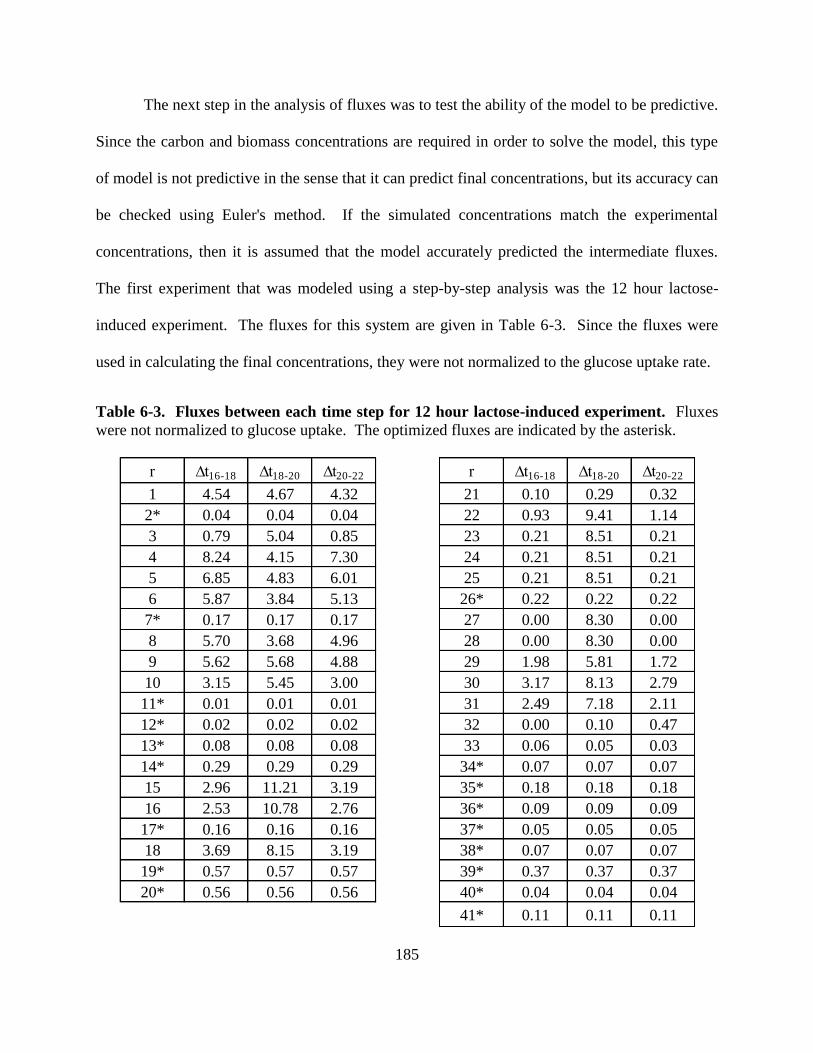
185
The next step in the analysis of fluxes was to test the ability of the model to be predictive.
Since the carbon and biomass concentrations are required in order to solve the model, this type
of model is not predictive in the sense that it can predict final concentrations, but its accuracy can
be checked using Euler's method. If the simulated concentrations match the experimental
concentrations, then it is assumed that the model accurately predicted the intermediate fluxes.
The first experiment that was modeled using a step-by-step analysis was the 12 hour lactose-
induced experiment. The fluxes for this system are given in Table 6-3. Since the fluxes were
used in calculating the final concentrations, they were not normalized to the glucose uptake rate.
Table 6-3. Fluxes between each time step for 12 hour lactose-induced experiment. Fluxes
were not normalized to glucose uptake. The optimized fluxes are indicated by the asterisk.
r ∆t16-18 ∆t18-20 ∆t20-22 r ∆t16-18 ∆t18-20 ∆t20-22
1 4.54 4.67 4.32 21 0.10 0.29 0.32
2* 0.04 0.04 0.04 22 0.93 9.41 1.14
3 0.79 5.04 0.85 23 0.21 8.51 0.21
4 8.24 4.15 7.30 24 0.21 8.51 0.21
5 6.85 4.83 6.01 25 0.21 8.51 0.21
6 5.87 3.84 5.13 26* 0.22 0.22 0.22
7* 0.17 0.17 0.17 27 0.00 8.30 0.00
8 5.70 3.68 4.96 28 0.00 8.30 0.00
9 5.62 5.68 4.88 29 1.98 5.81 1.72
10 3.15 5.45 3.00 30 3.17 8.13 2.79
11* 0.01 0.01 0.01 31 2.49 7.18 2.11
12* 0.02 0.02 0.02 32 0.00 0.10 0.47
13* 0.08 0.08 0.08 33 0.06 0.05 0.03
14* 0.29 0.29 0.29 34* 0.07 0.07 0.07
15 2.96 11.21 3.19 35* 0.18 0.18 0.18
16 2.53 10.78 2.76 36* 0.09 0.09 0.09
17* 0.16 0.16 0.16 37* 0.05 0.05 0.05
18 3.69 8.15 3.19 38* 0.07 0.07 0.07
19* 0.57 0.57 0.57 39* 0.37 0.37 0.37
20* 0.56 0.56 0.56 40* 0.04 0.04 0.04
41* 0.11 0.11 0.11

186
To calculate the predicted concentration at the next time step, the initial concentration
was used as described by Equation 4.16. The predicted concentrations for the 12 hour lactose-
induced experiment are shown in Table 6-4. Since the simulated concentrations for glucose and
acetate match the experimentally determined glucose and acetate concentrations, the model was
able to accurately predict the intermediate fluxes involved in metabolism. The simulated
concentrations for lactose were not as close of a match as those for glucose and acetate, but the
simulated values gave a decent estimation of the experimental concentrations.
Table 6-4. Predicted (simulated) versus experimental concentrations for 12 hr lactose-
induced experiment. Glu, ace, and lac refer to glucose, acetate, and lactose, respectively.
To check the ability of the model to predict the fluxes for other experiments, this process
was repeated for the IPTG-induced experiments and the auto-induced experiment with an
additional lactose pulse at 12 hours. In all instances, the model was able to accurately predict the
intermediate fluxes. However, the prediction of the lactose concentrations were not as good as
those for glucose and acetate in the experiment utilizing auto-induction with a lactose pulse. The
carbon concentrations for both IPTG-induced experiments were accurately predicted using the
fluxes. Table 6-5 gives the time step fluxes for both IPTG-induced experiments.
time exp glu exp ace exp lac sim glu sim ace sim lac
16 0 0.04 8.43 -- -- --
18 0 0.39 5.9 0 0.38 7.25
20 1.33 1.64 3.5 1.28 1.63 4.68
22 8.33 3.19 2.1 8.23 3.21 2.66

187
Table 6-5. Flux analysis for IPTG-induced experiments. The fluxes used in the optimization
routine are indicated by the asterisk.
r ∆t19-20 ∆t20-21 ∆t21-22 ∆t22-23 ∆t23-24 ∆t18-19 ∆t19-20 ∆t20-21 ∆t21-22 ∆t22-23
1 4.67 4.61 4.55 3.76 4.52 4.72 4.55 3.64 4.10 4.61
2* 0.04 0.04 0.04 0.04 0.04 0.04 0.04 0.04 0.04 0.04
3 5.03 4.95 4.86 3.28 4.82 1.22 0.77 0.62 0.69 1.20
4 4.25 4.19 4.10 3.50 4.07 8.17 8.15 5.85 7.01 7.91
5 3.74 4.87 4.76 2.66 4.72 9.73 6.76 4.71 5.75 6.72
6 5.16 3.87 3.78 3.91 3.75 3.16 5.79 3.99 4.90 5.73
7* 0.17 0.17 0.17 0.17 0.17 0.17 0.17 0.17 0.17 0.17
8 4.99 3.71 3.62 3.74 3.58 2.99 5.63 3.83 4.73 5.56
9 3.40 5.72 5.59 1.99 5.54 11.45 5.55 3.75 4.66 5.70
10 4.42 4.78 8.31 2.54 3.09 8.79 3.11 2.46 2.79 3.16
11* 0.01 0.01 0.01 0.01 0.01 0.01 0.01 0.01 0.01 0.01
12* 0.02 0.02 0.02 0.02 0.02 0.02 0.02 0.02 0.02 0.02
13* 0.08 0.08 0.08 0.08 0.08 0.08 0.08 0.08 0.08 0.08
14* 0.29 0.29 0.29 0.29 0.29 0.29 0.29 0.29 0.29 0.29
15 11.41 9.57 15.25 8.89 13.70 4.65 2.93 2.91 2.92 1.67
16 10.99 9.15 14.82 8.45 13.27 4.23 2.50 2.48 2.49 1.24
17* 0.16 0.16 0.16 0.16 0.16 0.16 0.16 0.16 0.16 0.16
18 7.37 8.50 8.75 5.40 10.72 6.56 3.53 2.25 2.89 3.63
19* 0.57 0.57 0.57 0.57 0.57 0.57 0.57 0.57 0.57 0.57
20* 0.56 0.56 0.56 0.56 0.56 0.56 0.56 0.56 0.56 0.56
21 0.05 0.04 0.04 0.01 0.03 0.07 0.07 0.00 0.03 0.05
22 9.38 9.22 9.04 6.15 8.92 1.74 0.90 0.85 0.87 1.73
23 8.70 8.56 8.38 5.51 8.26 1.05 0.21 0.21 0.21 1.06
24 8.70 8.56 8.38 5.51 8.27 1.05 0.21 0.21 0.21 1.06
25 8.70 8.56 8.38 5.51 8.26 1.05 0.21 0.21 0.21 1.06
26* 0.22 0.22 0.22 0.22 0.22 0.22 0.22 0.22 0.22 0.22
27 8.49 8.35 8.17 5.30 8.05 0.84 0.00 0.00 0.00 0.85
28 8.49 8.35 8.17 5.30 8.05 0.84 0.00 0.00 0.00 0.85
29 6.19 5.90 5.91 4.08 6.49 1.76 1.99 1.39 1.69 2.29
30 7.49 8.04 10.91 4.77 8.49 1.89 3.09 2.16 2.63 3.66
31 7.42 7.77 7.64 4.59 7.81 3.30 2.42 1.47 1.95 2.99
32 0.02 0.06 0.11 0.71 0.13 0.00 0.14 0.80 0.47 0.07
33 0.00 0.00 0.00 0.00 0.00 0.00 0.00 0.00 0.00 0.00
34* 0.07 0.07 0.07 0.07 0.07 0.07 0.07 0.07 0.07 0.07
35* 0.18 0.18 0.18 0.18 0.18 0.18 0.18 0.18 0.18 0.18
36* 0.09 0.09 0.09 0.09 0.09 0.09 0.09 0.09 0.09 0.09
37* 0.05 0.05 0.05 0.05 0.05 0.05 0.05 0.05 0.05 0.05
38* 0.07 0.07 0.07 0.07 0.07 0.07 0.07 0.07 0.07 0.07
39* 0.37 0.37 0.37 0.37 0.37 0.37 0.37 0.37 0.37 0.37
40* 0.04 0.04 0.04 0.04 0.04 0.04 0.04 0.04 0.04 0.04
41* 0.11 0.11 0.11 0.11 0.11 0.11 0.11 0.11 0.11 0.11
10 mM IPTG induction5 mM IPTG induction
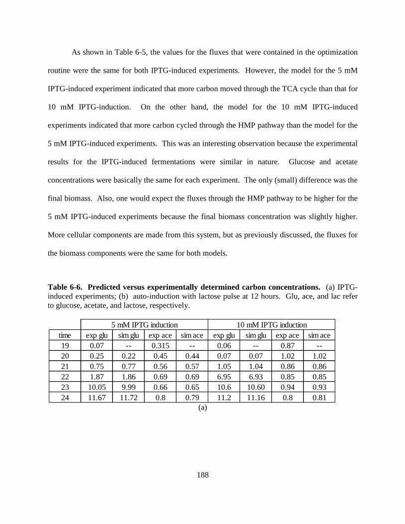
188
As shown in Table 6-5, the values for the fluxes that were contained in the optimization
routine were the same for both IPTG-induced experiments. However, the model for the 5 mM
IPTG-induced experiment indicated that more carbon moved through the TCA cycle than that for
10 mM IPTG-induction. On the other hand, the model for the 10 mM IPTG-induced
experiments indicated that more carbon cycled through the HMP pathway than the model for the
5 mM IPTG-induced experiments. This was an interesting observation because the experimental
results for the IPTG-induced fermentations were similar in nature. Glucose and acetate
concentrations were basically the same for each experiment. The only (small) difference was the
final biomass. Also, one would expect the fluxes through the HMP pathway to be higher for the
5 mM IPTG-induced experiments because the final biomass concentration was slightly higher.
More cellular components are made from this system, but as previously discussed, the fluxes for
the biomass components were the same for both models.
Table 6-6. Predicted versus experimentally determined carbon concentrations. (a) IPTG-
induced experiments; (b) auto-induction with lactose pulse at 12 hours. Glu, ace, and lac refer
to glucose, acetate, and lactose, respectively.
(a)
time exp glu sim glu exp ace sim ace exp glu sim glu exp ace sim ace
19 0.07 -- 0.315 -- 0.06 -- 0.87 --
20 0.25 0.22 0.45 0.44 0.07 0.07 1.02 1.02
21 0.75 0.77 0.56 0.57 1.05 1.04 0.86 0.86
22 1.87 1.86 0.69 0.69 6.95 6.93 0.85 0.85
23 10.05 9.99 0.66 0.65 10.6 10.60 0.94 0.93
24 11.67 11.72 0.8 0.79 11.2 11.16 0.8 0.81
5 mM IPTG induction 10 mM IPTG induction
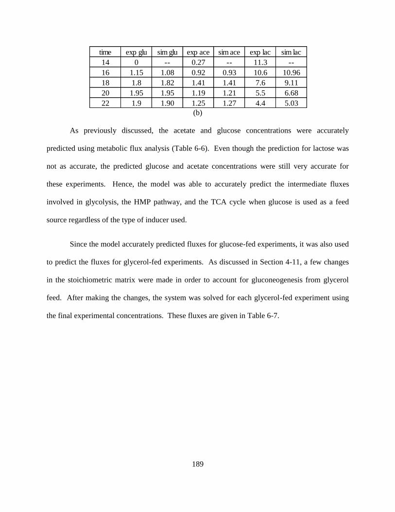
189
(b)
As previously discussed, the acetate and glucose concentrations were accurately
predicted using metabolic flux analysis (Table 6-6). Even though the prediction for lactose was
not as accurate, the predicted glucose and acetate concentrations were still very accurate for
these experiments. Hence, the model was able to accurately predict the intermediate fluxes
involved in glycolysis, the HMP pathway, and the TCA cycle when glucose is used as a feed
source regardless of the type of inducer used.
Since the model accurately predicted fluxes for glucose-fed experiments, it was also used
to predict the fluxes for glycerol-fed experiments. As discussed in Section 4-11, a few changes
in the stoichiometric matrix were made in order to account for gluconeogenesis from glycerol
feed. After making the changes, the system was solved for each glycerol-fed experiment using
the final experimental concentrations. These fluxes are given in Table 6-7.
time exp glu sim glu exp ace sim ace exp lac sim lac
14 0 -- 0.27 -- 11.3 --
16 1.15 1.08 0.92 0.93 10.6 10.96
18 1.8 1.82 1.41 1.41 7.6 9.11
20 1.95 1.95 1.19 1.21 5.5 6.68
22 1.9 1.90 1.25 1.27 4.4 5.03
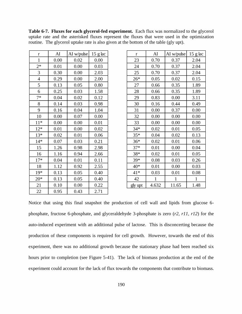
190
Table 6-7. Fluxes for each glycerol-fed experiment. Each flux was normalized to the glycerol
uptake rate and the asterisked fluxes represent the fluxes that were used in the optimization
routine. The glycerol uptake rate is also given at the bottom of the table (gly upt).
Notice that using this final snapshot the production of cell wall and lipids from glucose 6-
phosphate, fructose 6-phosphate, and glyceraldehyde 3-phosphate is zero (r2, r11, r12) for the
auto-induced experiment with an additional pulse of lactose. This is disconcerting because the
production of these components is required for cell growth. However, towards the end of this
experiment, there was no additional growth because the stationary phase had been reached six
hours prior to completion (see Figure 5-41). The lack of biomass production at the end of the
experiment could account for the lack of flux towards the components that contribute to biomass.
r AI AI w/pulse 15 g lac r AI AI w/pulse 15 g lac
1 0.00 0.02 0.00 23 0.70 0.37 2.04
2* 0.01 0.00 0.03 24 0.70 0.37 2.04
3 0.30 0.00 2.03 25 0.70 0.37 2.04
4 0.29 0.00 2.00 26* 0.05 0.02 0.15
5 0.13 0.05 0.80 27 0.66 0.35 1.89
6 0.25 0.03 1.58 28 0.66 0.35 1.89
7* 0.04 0.02 0.12 29 0.83 0.00 3.11
8 0.14 0.03 0.98 30 0.16 0.44 0.49
9 0.16 0.04 1.04 31 0.00 0.37 0.00
10 0.00 0.07 0.00 32 0.00 0.00 0.00
11* 0.00 0.00 0.01 33 0.00 0.00 0.00
12* 0.01 0.00 0.02 34* 0.02 0.01 0.05
13* 0.02 0.01 0.06 35* 0.04 0.02 0.13
14* 0.07 0.03 0.21 36* 0.02 0.01 0.06
15 1.26 0.98 2.98 37* 0.01 0.00 0.04
16 1.16 0.94 2.66 38* 0.02 0.01 0.05
17* 0.04 0.01 0.11 39* 0.08 0.03 0.26
18 1.12 0.92 2.55 40* 0.01 0.00 0.03
19* 0.13 0.05 0.40 41* 0.03 0.01 0.08
20* 0.13 0.05 0.40 42 1 1 1
21 0.10 0.00 0.22 gly upt 4.632 11.65 1.48
22 0.95 0.43 2.71

191
Additionally, the cell wall components can be synthesized from peptidoglycan, of which there is
a positive flux in Table 6-7 (Scheffers and Pinho, 2005).
Though it was not expected that the flux from glyceraldehydes 3-phosphate to fructose 6-
phosphate would be zero, it is not an uncommon occurrence for glucose fed-experiments (Lee et
al., 1997). This is also applicable for this glycerol-fed experiment since the fluxes have been
reversed. The optimal way for glucose to be metabolized is through the HMP pathway because
of the production of amino acids and nucleic acids that result from the processing of glucose
through this pathway. As indicated by the model, the flow of carbon bypassed the backbone
route in glycolysis and moved through the HMP pathway.
The same analysis was performed to check the accuracy of the model by comparing the
simulated carbon concentrations with the concentrations that were experimentally determined.
This analysis was performed on the auto-induced experiment and the experiment where 15 grams
of lactose was added when the glycerol feeding started. Table 6-8 shows this analysis.
Table 6-8. Predicted versus experimental concentrations for glycerol-fed experiments. (a)
Analysis for auto-induced experiments; (b) 15 grams of lactose at feed start analysis. Gly, ace,
and lac refer to glycerol, acetate, and lactose, respectively.
(a)
time exp gly sim gly exp ace sim ace exp lac sim lac
13 0.22 -- 0.07 -- 0.24 --
15 0.39 0.24 0.20 0.20 0 0.12
17 9.84 0.43 0.27 0.27 0 0
19 26.88 10.34 0.47 0.47 0 0
21 53.30 27.68 0.72 0.72 0 0
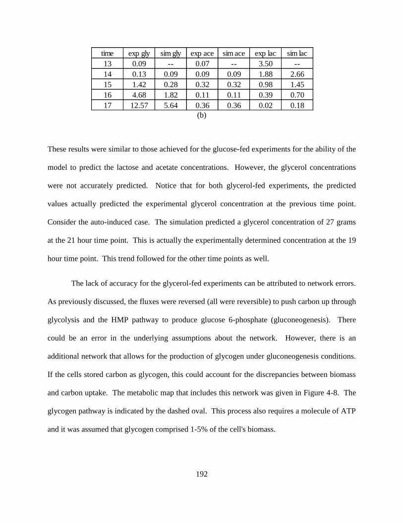
192
(b)
These results were similar to those achieved for the glucose-fed experiments for the ability of the
model to predict the lactose and acetate concentrations. However, the glycerol concentrations
were not accurately predicted. Notice that for both glycerol-fed experiments, the predicted
values actually predicted the experimental glycerol concentration at the previous time point.
Consider the auto-induced case. The simulation predicted a glycerol concentration of 27 grams
at the 21 hour time point. This is actually the experimentally determined concentration at the 19
hour time point. This trend followed for the other time points as well.
The lack of accuracy for the glycerol-fed experiments can be attributed to network errors.
As previously discussed, the fluxes were reversed (all were reversible) to push carbon up through
glycolysis and the HMP pathway to produce glucose 6-phosphate (gluconeogenesis). There
could be an error in the underlying assumptions about the network. However, there is an
additional network that allows for the production of glycogen under gluconeogenesis conditions.
If the cells stored carbon as glycogen, this could account for the discrepancies between biomass
and carbon uptake. The metabolic map that includes this network was given in Figure 4-8. The
glycogen pathway is indicated by the dashed oval. This process also requires a molecule of ATP
and it was assumed that glycogen comprised 1-5% of the cell's biomass.
time exp gly sim gly exp ace sim ace exp lac sim lac
13 0.09 -- 0.07 -- 3.50 --
14 0.13 0.09 0.09 0.09 1.88 2.66
15 1.42 0.28 0.32 0.32 0.98 1.45
16 4.68 1.82 0.11 0.11 0.39 0.70
17 12.57 5.64 0.36 0.36 0.02 0.18
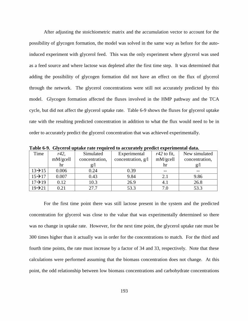
193
After adjusting the stoichiometric matrix and the accumulation vector to account for the
possibility of glycogen formation, the model was solved in the same way as before for the auto-
induced experiment with glycerol feed. This was the only experiment where glycerol was used
as a feed source and where lactose was depleted after the first time step. It was determined that
adding the possibility of glycogen formation did not have an effect on the flux of glycerol
through the network. The glycerol concentrations were still not accurately predicted by this
model. Glycogen formation affected the fluxes involved in the HMP pathway and the TCA
cycle, but did not affect the glycerol uptake rate. Table 6-9 shows the fluxes for glycerol uptake
rate with the resulting predicted concentration in addition to what the flux would need to be in
order to accurately predict the glycerol concentration that was achieved experimentally.
Table 6-9. Glycerol uptake rate required to accurately predict experimental data.
Time r42,
mM/gcell
hr
Simulated
concentration,
g/l
Experimental
concentration, g/l
r42 to fit,
mM/gcell
hr
New simulated
concentration,
g/l
1315 0.006 0.24 0.39 -- --
1517 0.007 0.43 9.84 2.1 9.86
1719 0.12 10.3 26.9 4.1 26.8
1921 0.21 27.7 53.3 7.0 53.3
For the first time point there was still lactose present in the system and the predicted
concentration for glycerol was close to the value that was experimentally determined so there
was no change in uptake rate. However, for the next time point, the glycerol uptake rate must be
300 times higher than it actually was in order for the concentrations to match. For the third and
fourth time points, the rate must increase by a factor of 34 and 33, respectively. Note that these
calculations were performed assuming that the biomass concentration does not change. At this
point, the odd relationship between low biomass concentrations and carbohydrate concentrations

194
comes to light. According to the model, with the given biomass concentrations, the glycerol
concentrations remaining in the media should be much higher than they actually were.
The last calculation that was performed using the results from metabolic flux analysis
was cellular yield from ATP in an attempt to further investigate the large differences in overall
biomass yield. The fluxes that were involved in these calculations are given in Table 6-10 for all
experiments using the un-regulated exponential feeding profile. The results from the
calculations (refer to Equations 4.17 to 4.21) are given in Table 6-11.
Table 6-10. Fluxes used in yield of biomass from ATP calculations.
Table 6-11. Contributions of energetics to ATP fluxes and biomass yield from ATP.
AI AI w/pulse feed start
4 G6P to R5P 8.03 7.66 3.96 10.16 6.44 3.14 1.36 0.00 2.96
10 F6P to G3P 3.12 2.98 4.30 3.95 4.89 4.86 0.00 0.81 0.00
15 G3P to 3PG 3.01 2.93 10.10 3.78 18.55 7.14 5.84 11.36 4.41
18 PEP to Pyr 3.51 3.26 7.21 4.55 15.83 2.75 5.20 10.72 3.78
21 AcCoA to Acetate 0.15 0.06 0.06 0.22 0.14 0.07 0.48 0.00 0.32
22 Pyr to AcCoA 0.97 0.89 8.41 1.24 14.20 6.99 4.42 5.02 4.02
24 Cit to Iso 0.21 0.21 7.73 0.26 13.12 6.46 3.26 4.34 3.03
27 KG to Succ 0.00 0.00 7.52 0.00 12.80 6.30 3.04 4.11 2.80
28 Succ to Mal 0.00 0.00 7.52 0.00 12.80 6.30 3.04 4.11 2.80
29 Mal to OA 1.95 1.86 5.47 2.44 9.52 4.62 3.84 0.00 4.61
31 Mal to Pyr 2.38 2.22 6.48 3.06 8.96 4.36 0.00 4.36 0.00
33 Lac to G6P 0.00 0.00 0.00 0.07 0.00 0.00 0.00 0.01 0.00
42 Gly to G3P 0.00 0.00 0.00 0.00 0.00 0.00 4.63 11.65 1.48
Glycerol
DescriptionAI
Lac at
feed startr
12 hr lac
induction
5 mm
IPTG
10 mM
IPTG
AI
w/pulse
AI AI w pulse 15 g lac
FADH 0.0 0.0 7.5 0.0 12.8 6.3 3.0 4.1 2.8
NADPH 24.6 23.4 53.6 31.1 90.0 42.2 23.1 29.2 24.8
ATP 3.5 3.3 20.6 4.5 42.4 11.4 9.9 15.3 9.8
ATP total 35.5 33.7 96.8 45.0 170.5 71.7 42.6 56.8 44.5
D 0.19 0.19 0.19 0.24 0.30 0.14 0.03 0.05 0.12
Y cell/ATP 5.4 5.6 2.0 5.3 1.8 2.0 0.7 0.9 2.7
Biomass 60 76 70 33 41 43 35 19 19
Glycerol12 hr lac
induction
5 mm
IPTG
10 mM
IPTG
AI
w/pulseAI
Lac at
feed start

195
Notice that the total amount of ATP produced for the 10 mM IPTG-induced and the lactose-
induced at feed start experiments was very high compared to other experiments. Since biomass
yield from ATP is inversely proportional to ATP production, their yields were lower. Also, the
biomass yield from ATP for the glycerol-fed experiments were low (due to the low biomass
concentrations. Next, the ratios of biomasses were compared to the ratios of biomass yield from
ATP to see how closely these two are related. This analysis provided information as to why
there were large differences in biomass production. If the ATP yield ratios match the biomass
ratios, then the metabolic pathways that contribute to this difference can be identified.
As shown in Table 6-12, the ratios for a few of the experiments were practically the
same, but for most they were different. For example, the ratios for the 5 mM IPTG-induced
experiment and the 12 hr lactose-induced experiment were very similar (1.1 vs. 1.3), but the
ratios for the 12 hr lactose-induced experiment to the auto-induced experiment with glycerol feed
were very different (7.7 vs. 1.7). The highlighted ratios are those in which the percent error is
less than or equal to 20%. (Refer to Section 9.9 for the complete table of percent error.) The
differences can be accounted for by the total ATP fluxes in Table 6-11 (from the individual
fluxes in Table 6-10).
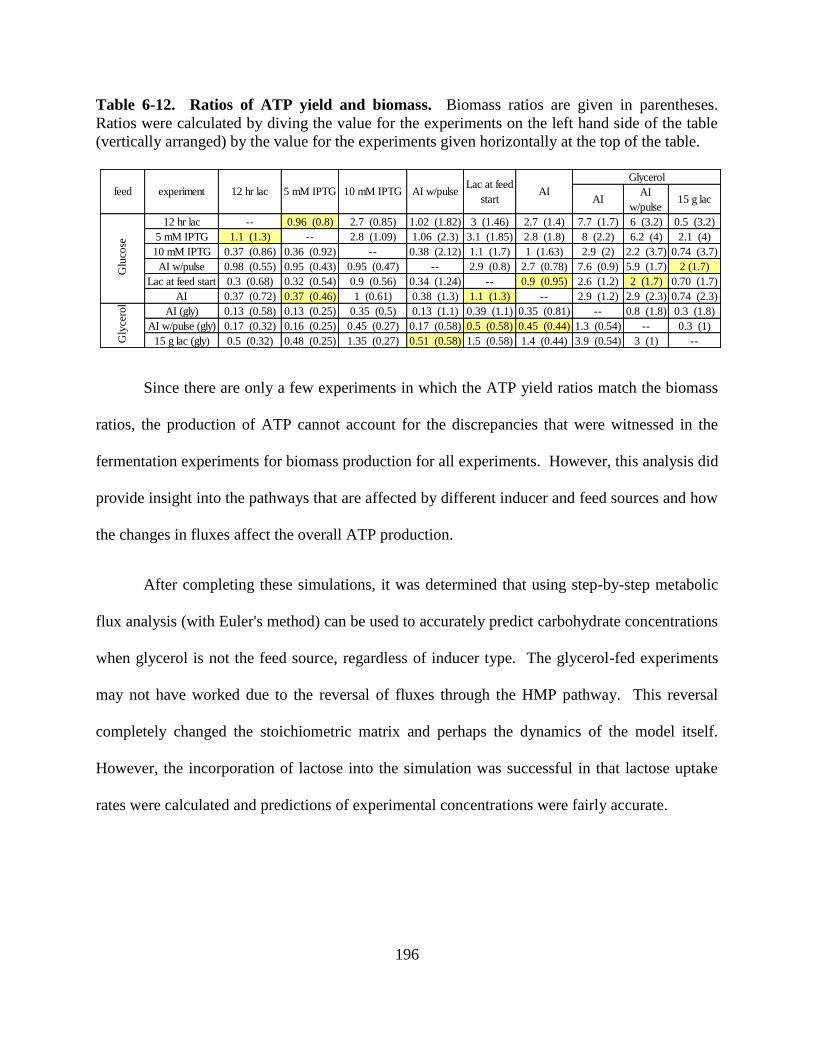
196
Table 6-12. Ratios of ATP yield and biomass. Biomass ratios are given in parentheses.
Ratios were calculated by diving the value for the experiments on the left hand side of the table
(vertically arranged) by the value for the experiments given horizontally at the top of the table.
Since there are only a few experiments in which the ATP yield ratios match the biomass
ratios, the production of ATP cannot account for the discrepancies that were witnessed in the
fermentation experiments for biomass production for all experiments. However, this analysis did
provide insight into the pathways that are affected by different inducer and feed sources and how
the changes in fluxes affect the overall ATP production.
After completing these simulations, it was determined that using step-by-step metabolic
flux analysis (with Euler's method) can be used to accurately predict carbohydrate concentrations
when glycerol is not the feed source, regardless of inducer type. The glycerol-fed experiments
may not have worked due to the reversal of fluxes through the HMP pathway. This reversal
completely changed the stoichiometric matrix and perhaps the dynamics of the model itself.
However, the incorporation of lactose into the simulation was successful in that lactose uptake
rates were calculated and predictions of experimental concentrations were fairly accurate.
12 hr lac -- 0.96 (0.8) 2.7 (0.85) 1.02 (1.82) 3 (1.46) 2.7 (1.4) 7.7 (1.7) 6 (3.2) 0.5 (3.2)
5 mM IPTG 1.1 (1.3) -- 2.8 (1.09) 1.06 (2.3) 3.1 (1.85) 2.8 (1.8) 8 (2.2) 6.2 (4) 2.1 (4)
10 mM IPTG 0.37 (0.86) 0.36 (0.92) -- 0.38 (2.12) 1.1 (1.7) 1 (1.63) 2.9 (2) 2.2 (3.7) 0.74 (3.7)
AI w/pulse 0.98 (0.55) 0.95 (0.43) 0.95 (0.47) -- 2.9 (0.8) 2.7 (0.78) 7.6 (0.9) 5.9 (1.7) 2 (1.7)
Lac at feed start 0.3 (0.68) 0.32 (0.54) 0.9 (0.56) 0.34 (1.24) -- 0.9 (0.95) 2.6 (1.2) 2 (1.7) 0.70 (1.7)
AI 0.37 (0.72) 0.37 (0.46) 1 (0.61) 0.38 (1.3) 1.1 (1.3) -- 2.9 (1.2) 2.9 (2.3) 0.74 (2.3)
AI (gly) 0.13 (0.58) 0.13 (0.25) 0.35 (0.5) 0.13 (1.1) 0.39 (1.1) 0.35 (0.81) -- 0.8 (1.8) 0.3 (1.8)
AI w/pulse (gly) 0.17 (0.32) 0.16 (0.25) 0.45 (0.27) 0.17 (0.58) 0.5 (0.58) 0.45 (0.44) 1.3 (0.54) -- 0.3 (1)
15 g lac (gly) 0.5 (0.32) 0.48 (0.25) 1.35 (0.27) 0.51 (0.58) 1.5 (0.58) 1.4 (0.44) 3.9 (0.54) 3 (1) --Gly
cero
lG
luco
se
AIAI
w/pulse15 g lac
Glycerol
feed experiment 12 hr lac 5 mM IPTG 10 mM IPTG AI w/pulseLac at feed
startAI

197
7. Conclusions and recommendations
Overall, fed-batch fermentation is a viable option for production of GST-PTH-CBD and
the methods developed here would work well with the production of other therapeutic fusion
proteins. The media development method utilized in this dissertation can be adapted to the
production of other proteins by examining their amino acid content and it is novel in the sense
that all components remain defined in nature. The feeding profile developed in this dissertation
would also work for fed-batch cultivations of other strains of Escherichia coli. However, the
feeding profile should be modified if using a carbon substrate other than glucose. This would
prevent the likely accumulation of other substrates, since glucose is taken up more rapidly by the
cells that other carbon sources.
Additionally, in many of the experiments, it became apparent that lactose has an effect on
the utilization of glucose. Growth became inhibited, but glucose uptake did not stop. This
phenomenon could be further examined by using fed-batch fermentation with lactose induction
for other systems that contain the lac operon. Insight into this particular relationship between
carbohydrates and corresponding biomass production was lacking in the literature. In short, the
following trends were observed for fed-batch fermentation experiments:
Product yield from biomass remained constant for the duration of the fermentation for
most experiments.
Acetate concentrations remained well below inhibitory values, due to the design of the
feeding profile.
Lactose added earlier on negatively affected biomass yield and lactose was consumed
regardless of the presence of glucose.
198
The following statements are brief recommendations for the fermentation experiments:
To make the most cells, cultures should be induced with IPTG.
To make the most product, cultures should be auto-induced and fed with glycerol.
To make the most product with cost in mind, cultures should be auto-induced and fed
with glycerol or auto-induced with an additional lactose pulse and fed with glucose.
Dynamic modeling for this system using the traditional types of equations did not work.
The feed, volume, and biomass equations were a close fit to those experimentally observed. The
final simulated lactose concentrations tracked with experimentally observed concentrations, but
the slope of degradation was not a good fit. However, the simulation modeling the complete
fermentation system was unable to accurately predict the glucose and acetate concentrations. It
appears that under lactose induction, the relationship between the three carbohydrates for this
expression system is unique.
Lastly, metabolic flux analysis was used to track the movement of carbon through
metabolism in an attempt to identify the ‘carbon sink’ that was experimentally observed. This
tool can be used to gain valuable insight into cellular metabolism with regards to the production
of biomass using this particular construct. This type of modeling can be use to predict
intermediate fluxes if some information is known about the external environment of the cell.
Other systems using lactose as an inducer could be examined using metabolic flux analysis to
further describe the relationship between carbohydrates and biomass production.
After a complete analysis of the data from metabolic flux analysis and the experiments, a
final additional recommendation would be to examine the metabolism of a lac deficient strain. If
lactose was used as an inducer, but it was unable to be metabolized, it may act more like IPTG in
199
the sense that growth is not affected. Then, the best of both cases would hold true - higher cell
densities (as in the IPTG-induced experiments) with high protein yield from cells (as in the case
of lactose-induced experiments).

200
8. References
Akesson, M., Hagander, P., & Axelsson, J. P. (2001) Avoiding acetate accumulation in
Escherichia coli cultures using feedback control of glucose feeding. Biotechnology and
Bioengineering. 73, 223-230.
Antoniewicz, M., Kranie, D., Laffend, L., Gozalez-Lergier, J., Kelleher, J., & Stephanopoulos,
G. (2007) Metabolic flux analysis in a nonstationary system: Fed-batch fermentation of a
high yielding strain of E. coli producing 1,3-propanediol. Metabolic engineering. 9, 277-
292.
Aristidou, A., San, K., & Bennett, G. (1995) Metabolic engineering of Escherichia coli to
enhance recombinant protein production through acetate reduction. Biotechnol. Prog. 11,
475-478.
Aucoin, M., McMurray-Beaulieu, V., Poulin, F., Boivin, E., Chen, J., Ardelean, F., Cloutier, M.,
Choi, Y., Miguez, C., & Jolicoeur, M. (2006) Identifying conditions for inducible protein
production in E. coli: Combining a fed-batch and multiple induction approach. Microbial
Cell Factories. 5, 27.
Babaeipour, V., Shojaosadati, S. A., Khalilzadeh, R., Maghsoudi, N., & Tabandeh, F. (2008) A
proposed feeding strategy for the overproduction of recombinant proteins in Escherichia
coli. Biotechnology and applied biochemistry. 49, 141.
Behme, S. (2009) Manufacturing of pharmaceutical proteins: From technology to economy.
WILEY-VCH Verlag GmbH & Co, KGaA, Weinheim
Berrow, N., Bussow, K., Coutard, B., Diprose, J., Ekberg, M., Folkers, G. E., Levy, N., Lieu, V.,
Owens, R. J., Peleg, Y., Pinaglia, C., Quevillon-Cheruel, S., Salim, L., Scheich, C.,
Vincentelli, R., & Busso, D. (2006) Recombinant protein expression and solubility
screening in Escherchia coli: A comparative study. Biological Crystallography. 62, 1218-
1226.
Blommel, P. G., Becker, K., J., Duvnjak, P., & Fox, B. (2007) Enhanced bacterial protein
expression during auto-induction obtained by alteration of lac Repressor dosage and
medium composition. Biotechnol. Prog. 23, 585-598.
Camps, M. (2010) Modulation of ColE1-like plasmid replication for recombinant gene
expression. Recent patents on DNA & gene sequences. 4, 58.
Carpenter, G., Stoscheck, C. M., & Soderquist, A. M. (1982) EPIDERMAL GROWTH
FACTOR*. Annals of the New York Academy of Sciences. 397, 11-17.
Chassagnole, C., Noisommit-Rizzi, N., Schmid, J. W., Mauch, K., & Reuss, M. (2002) Dynamic
modeling of the central carbon metabolism of Escherichia coli. Biotechnology and
bioengineering. 79, 53-73.
201
Chen, Q., Bentley, W. E., & Weigand, W. A. (1995) Optimization for a recombinant E. coli fed-
batch fermentation. Applied Biochemistry and Biotechnology. 51/52, 449-461.
Chen, W., Bailey, J., & Lee, S. (1991) Molecular design of expression systems: Comparison of
different repressor control configurations using molecular mechanism models. Biotech and
Bioeng. 38, 679-687.
Chen, W., Graham, C., & Ciccarelli, R. (1997) Automated fed-batch fermentation with feed-back
controls based on dissolved oxygen (DO) and pH for production of DNA vaccines. Journal
of Industrial Microbiology & Biotechnology. 18, 43-48.
Chen, W., Shi, C., Yi, S., Chen, B., Zhang, W., Fang, Z., Wei, Z., Jiang, S., Sun, X., Hou, X.,
Xiao, Z., Ye, G., & Dai, J. (2010) Bladder regeneration by collagen scaffolds with collagen
binding human basic fibroblast growth factor. The Journal of Urology. 183, 2432-2439.
Cheng, B., Fournier, R., Relue, P., & Schisler, J. (2001) An experimental and theoretical study of
the inhibition of Escherichia coli lac operon gene expression by antigene oligonucleotides.
Biotechnology and Bioengineering. 74, 220-229.
Choi, J. H., Keum, K. C., & Lee, S. Y. (2006) Production of recombinant proteins by high cell
density culture of Escherichia coli. Chemical Engineering Science. 61, 876-885.
Cockshott, A. R., & Bogle, I. D. L. (1999) Modelling the effects of glucose feeding on a
recombinant E. coli fermentation. Bioprocess Engineering. 20, 83-90.
Covert, M. W., Schilling, C. H., & Palsson, B. (2001) Regulation of gene expression in flux
balance models of metabolism. Journal of theoretical biology. 213, 73-88.
de Mare, L., Velut, S., Ledung, E., Cimander, C., Norrman, B., Nordberg Karlsson, E., Holst, O.,
& Hagander, P. (2005) A cultivation technique for E. coli fed-batch cultivations operating
close to the maximum oxygen transfer capacity of the reactor. Biotechnology Letters. 27,
983-990.
De Mey, M., De Maeseneire, S., Soetaert, W., & Vandamme, E. (2007) Minimizing acetate
formation in E. coli fermentations. J Ind Microbiol Biotechnol. 34, 689-700.
Donovan, R., Robinson, R., CW, & Glick, B. (1996) Review: Optimizing inducer and culture
conditions for expression of foreign proteins under the control of the lac promoter. Journal
of Industrial Microbiology. 16, 145-154.
Dubach, A., & Markl, H. (1992) Application of an extended kilman filter method for monitoring
high cell density cultivation of Escherichia coli. Journal of Fermentation and
Bioengineering. 73, 396-402.
Eiteman, M., & Altman, E. (2006) Overcoming acetate in Escherichia coli recombinant protein
fermentations. Trends in Biotechnology. 24, 530-536.

202
Fan, D., Luo, Y., Mi, Y., Ma, X., & Shang, L. (2005) Characteristics of fed-batch cultures of
recombinant Escherichia coli containing human-like collagen cDNA at different specific
growth rates. Biotechnology Letters. 27, 865-870.
Faulkner, E., Barrett, M., Okor, S., Kieran, P., Casey, E., Paradisi, F., Engel, P., & Gennon, B.
(2006) Use of fed-batch cultivation for achieving high cell densities for the pilot-scale
production of a recombinant protein (phenylalanine dehydrogenase) in Escherichia coli.
Biotechnol. Prog. 22, 889-897.
Ferrer-Miralles, N., Domingo-Espin, J., Corchero, J., Vazquez, E., & Villaverde, A. (2009)
Microbial factories for recombinant pharmaceuticals. Microbial Cell Factories. 8, 17.
Fu, X., Tong, W., & Wei, D. (2005) Extracellular production of human parathyroid hormone as a
thiooredoxin fusion form in Escherichia coli by chemical permeabilization combined with
heat treatment. Biotechnol Prog. 21, 1429-1435.
Garcia-Arrazola, R., Siu, S. C., Chan, G., Buchanan, I., Doyle, B., Titchener-Hooker, N., &
Baganz, F. (2005) Evaluation of a pH-stat feeding strategy on the production and recovery
of fab' fragments from E. coli. Biochemical Engineering Journal. 25, 221-230.
Gombert, A. K., & Kilikian, B. V. (1998) Recombinant gene expression in Escherichia coli
cultivation using lactose as an inducer. Journal of Biotechnology. 60, 47-54.
Grabski, A., Mehler, M., & Drott, D. (2005) The overnight express autoinduction system: High-
density cell growth and protein expression
while you sleep. Nature Methods. 2, 233-235.
Han, K., Lim, H. C., & Hong, J. (1992) Acetic acid formation in Escherichia coli fermentation.
Biotech and Bioneng. 39, 663-671.
Hannachi Imen, E., Nakamura, M., Mie, M., & Kobatake, E. (2009) Construction of
multifunctional proteins for tissue engineering: Epidermal growth factor with collagen
binding and cell adhesive activities. Journal of Biotechnology. 139, 19-25.
Harder, M. P. F., Sanders, E. A., Wingender, E., & Deckwer, W. (1993) Studies on the
production of human parathyroid hormone by recombinant Escherichia coli. Appl
Microbiol Biotechnol. 39, 329-334.
Hoffman, B. J., Broadwater, J. A., Johnson, P., Harper, J., Fox, B. G., & Kenealy, W. R. (1995)
Lactose fed-batch overexpression of recombinant metalloproteins in Escherichia coli
BL21(DE3): Process control yielding high levels of metal-incorporated, soluble protein.
Protein expression and purification. 6, 646-654.
Holms, W. H. (1986) The central metabolic pathways of Escherichia coli: Relationship between
flux and control at a branch point, efficiency of conversion to biomass, and excretion of
acetate. Current Topics in Cellular Regulation. 28, 59-105.
203
Hong, W. K., Kwon, S. J., & Kim, E. K. (1992) Effects of in-vitro protein stabilizers on the
overproduction of recombinant beta-lactamase in Escherichia coli. Biotechnol. Lett. 14,
345-350.
Jacoby, G. A., & Sutton, L. (1985) Beta-lactamases and beta-lactam resistance in Escherichia
coli. Antimicrobial agents and chemotherapy. 28, 703-705.
Jenzsch, M., Simutis, R., & Luebbert, A. (2006) Generic model control of the specific growth
rate in recombinant Escherichia coli cultivations. Journal of Biotechnology. 122, 483-493.
Kauffman, K. J., Prakash, P., & Edwards, J. S. (2003) Advances in flux balance analysis.
Current opinion in biotechnology. 14, 491-496.
Kayser, A., Weber, J., Volker, H., & Rinas, U. (2005) Metabolic flux analysis of Escherichia
coli in glucose-limited continuous culture. I. growth-rate-dependent metabolic efficiency at
steady state. Microbiology. 151, 693-706.
Kilikian, B., Suarez, I., Liria, C., & Gombert, A. K. (2000) Process strategies to improve
heterologous protein production in Escherichia coli under lactose or IPTG induction.
Process Biochemistry. 35, 1019-1025.
Kim, B. S., Lee, S. C., Lee, S. Y., Chang, Y. K., & Chang, H. N. (2004) High cell density fed-
batch cultivation of Escherichia coli using exponential feeding combined with pH-stat.
Bioprocess Biosyst Eng. 26, 147-150.
Kim, M., Elvin, C., Brownlee, A., & Lyons, R. (2007) High yield expression of recombinant pro-
resilin: Lactose-induced fermentation in E. coli and facile purification. Protein Expr. Purif.
52, 230-236.
Kleman, G. L., Chalmers, J. J., Luli, G. W., & Strohl, W. R. (1991) A predictive and feedback
control algorithm maintains a constant glucose concentration in fed-batch fermentations.
Applied and Environmental Microbiology. 57, 910-917.
Kleman, G. L., & Strohl, W. R. (1994) Acetate metabolism by Escherichia coli in high-cell-
density fermentation. Applied and Environmental Microbiology. 60, 3952-3958.
Koffas, M., Roberge, C., Lee, K., & Stephanopoulos, G. (1999) Metabolic engineering. Annual
Review of Biomedical Engineering. 1, 535-557.
Korz, D. J., Rinas, U., Hellmuth, K., Sanders, E. A., & Deckwer, W. (1995) Simple fed-batch
technique for high cell density cultivation of Escherichia coli. Journal of Biotechnology.
39, 59-65.
Kosinski, M. J., Rinas, U., & Bailey, J. E. (1992) Isopropyl-β-D-thiogalactopyranoside
influences the metabolism of Escherichia coli. Applied Microbiology and Biotechnology.
36, 782-784.
204
Kotik, M., Kocanova, M., Maresova, H., & Kyslik, P. (2004) High-level expression of a fungal
pyranose oxidase in high cell-density fed-batch cultivations of Escherichia coli using
lactose as inducer. Protein expression and purification. 36, 61-69.
Kremling, A., Bettenbrock, K., Laube, B., Jahreis, K., Lengeler, J. W., & Gilles, E. D. (2001)
The organization of metabolic reaction networks: application for diauxic growth on
glucose and lactose. Metab. Eng. 3, 362-379.
Kweon, D., Han, N. S., Park, K., & Seo, J. (2001) Overproduction of phytolacca insularis protein
in batch and fed-batch culture of recombinant Escherichia coli. Process Biochemistry. 36,
537-542.
Kwon, S., Kim, S., & Kim, E. (1996) Effects of glycerol on beta-lactamase production during
high cell density cultivation of recombinant Escherichia coli. Biotechnology progress. 12,
205-208.
Lee, J., Goel, A., Ataai, M., & Domach, M. (1997) Supply-side analysis of growth of bacillus
subtilis on glucose-citrate medium: Feasible network alternatives and yield optimality.
Applied and Environmental Microbiology. 63, 710-718.
Lee, S. Y. (1996) High cell-density culture of Escherichia coli. Trends in biotechnology. 14, 98-
105.
Levisauskas, D., & Tekoris, T. (2005) Model-based optimization of fed-batch fermentation
processes using predetermined type feed-rate time profiles. A comparative study.
Information Technology and Control. 34, 231-236.
Li, Z., Kessler, W., van den Heuvel, J., & Rinas, U. (2011) Simple defined autoinduction
medium for high-level recombinant protein productino using T7-based Escherichia coli
expression systems. Appl Microbiol Biotechnol. 91, 1203-1213.
Lin, Y. H., & Neubauer, P. (2000) Influence of controlled glucose oscillations on a fed-batch
process of recombinant Escherichia coli. Journal of Biotechnology. 79, 27-37.
Liu, Q., Lin, J., Liu, M., Tao, X., Wei, D., Ma, X., & Yang, S. (2007) Large scale preparation of
recombinant human parathyroid hormone 1–84 from Escherichia coli. Protein expression
and purification. 54, 212-219.
Longobardi, G. P. (1994) Fed-batch versus batch fermentation. Bioprocess Engineering. 10, 185-
194.
Macaloney, G., Hall, J. W., Rollins, M. J., Draper, I., Anderson, K. B., Preston, J., Thompson, B.
G., & McNeil, B. (1997) The utility and performance of near-infra red spectroscopy in
simultaneous monitoring of multiple components in a high cell density recombinant
Escherichia coli production process. Bioprocess Engineering. 17, 157-167.

205
Matsushita, O., Jung, C., Minami, J., Katayama, S., Nishi, N., & Okabe, A. (1998) A study of the
collagen-binding domain of a 116-kDa clostridium histolyticum collagenase*. The Journal
of Biological Chemistry. 273, 3643-3648.
Meadows, A. L., Karnik, R., Lam, H., Forestell, S., & Snedecor, B. (2010) Application of
dynamic flux balance analysis to an industrial Escherichia coli fermentation. Metabolic
engineering. 12, 150-160.
Menzella, H., Ceccarelli, E., & Gramajo, H. (2003) Novel Escherichia coli strain allows efficient
recombinant protein production using lactose as inducer. Biotech and Bioneng. 82, 809-817.
Mohseni, S., Babaeipour, V., & Vali, A. (2009) Design of sliding mode controller for the optimal
control of fed-batch cultivation of recombinant E.coli. Chemical Engineering Science. 64,
4433-4441.
Murarka, A., Dharmadi, Y., Yazdani, S. S., & Gonzalez, R. (2008) Fermentative utilization of
glycerol by Escherichia coli and its implications for the production of fuels and chemicals.
Applied and Environmental Microbiology. 74, 1124-1135.
Namdev, P. K., Irwin, N., Thompson, B., & Gray, M. R. (1993) Effect of oxygen fluctuations on
recombinant Escherichia coli fermentation. Biotechnology and bioengineering. 41, 666-
670.
Neubauer, P., Hofmann, K., Holst, O., Mattiasson, B., & Kruschke, P. (1992) Maximizing the
expression of a recombinant gene in Escherichia coli by manipulation of induction time
using lactose as inducer. Appl Microbiol Biotechnol. 36, 739-744.
Neubauer, P., Häggström, L., & Enfors, S. (1995) Influence of substrate oscillations on acetate
formation and growth yield in Escherichia coli glucose limited fed-batch cultivations.
Biotechnology and bioengineering. 47, 139-146.
Nozomu, N., Matsushita, O., Yuube, K., Miyanaka, H., Okabe, A., & Wada, F. (1998) Collagen-
binding growth factors: Production and characterization of functional fusion proteins
having a collagen-binding domain. Proceedings of the National Academy of Sciences of the
United States of America. 95, 7018-7023.
Panda, A. K., Khan, R. H., Mishra, S., Appa Rao, K. B. C., & Totey, S. M. (2000) Influences of
yeast extract on specific cellular yield of ovine growth hormone during fed-batch
fermentation of E. coli. Bioprocess Engineering. 22, 379-383.
Pramanik, J., & Keasling, J. D. (1997) Stoichiometric model of Escherichia coli metabolism:
Incorporation of growth-rate dependent biomass composition and mechanistic energy
requirements. Biotech and Bioeng. 56, 398-421.
Ramchuran, S., Holst, O., & Karlsson, E. (2005) Effect of postinduction nutrient feed
composition and use of lactose as inducer during production of thermostable xylanase in

206
Escherchia coli glucose-limited fed-batch cultivations. Journal of Bioscience and
Bioengineering. 99, 477-484.
Roeva, O., Pencheva, T., Tzonkov, S., Arndt, M., Hitzmann, B., Kleist, S., Miksch, G., & Friehs,
K. (2007) Multiple model approach to modelling of Escherichia coli fed-batch cultivation
extracellular production of bacterial phytase. Electronic Journal of Biotechnology. 10, 593-
603.
Roeve, O., & Tzonkov, S. (2006) Modelling of Escherichia coli cultivations: Acetate inhibition
in a fed-batch culture. Bioautomation. 4, 1-11.
Sakon, J., Gensure, R. C., & Matsushita, O. (2010) Fusion proteins of collagen-binding domain
and parathyroid hormone. 20100129341
Sandén, A. M., Prytz, I., Tubulekas, I., Förberg, C., Le, H., Hektor, A., Neubauer, P., Pragai, Z.,
Harwood, C., Ward, A., Picon, A., de Mattos, J. T., Postma, P., Farewell, A., Nyström, T.,
Reeh, S., Pedersen, S., & Larsson, G. (2003) Limiting factors in Escherichia coli fed-batch
production of recombinant proteins. Biotechnology and bioengineering. 81, 158-166.
Santillan, M. (2008) Bistable behavior in a model of the lac operon in Escherichia coli with
variable growth rate. Biophysical Journal. 94, 2065-2081.
Santillan, M., & Mackey, M. C. (2008) Quantitative approaches to the study of bistability in the
lac operon of Escherichia coli. J. R. Soc. Interface. 5, S29-S39.
Sassenfeld, H. M. (1990) Engineering proteins for purification. Trends in biotechnology. 8, 88-
93.
Sauer, U. (2006) Metabolic networks in motion: 13
C-based flux analysis. Molecular Systems
Biology. 14, 1-10.
Sauer, U., Lasko, D. R., Fiaux, J., Hochuli, M., Glaser, R., Szyperski, T., Wüthrich, K., &
Bailey, J. E. (1999) Metabolic flux ratio analysis of genetic and environmental modulations
of Escherichia coli central carbon metabolism. Journal of Bacteriology. 181, 6679-6688.
Scheffers, D., & Pinho, M. G. (2005) Bacterial cell wall synthesis: New insights from
localization studies. Microbiology and molecular biology reviews. 69, 585-607.
Shi, C., Chen, W., Zhao, Y., Chen, B., Xiao, Z., Wei, Z., Hou, X., Tang, J., Wang, Z., & Dai, J.
(2011) Regeneration of full-thickness abdominal wall defects in rats using collagen
scaffolds loaded with collagen-binding basic fibroblast growth factor. Biomaterials. 32,
753-759.
Shiloach, J., Kaufman, J., Guillard, A. S., & Fass, R. (1996) Effect of glucose supply strategy on
acetate accumulation, growth, and recombinant protein production by Escherichia coli
207
BL21 ("lambda" DE3) and escherichia coli JM109. Biotechnology and Bioengineering. 49,
421-428.
Shiloach, J., & Fass, R. (2005) Growing E. coli to high cell density - A historical perspective on
method development. Biotechnology Advances. 23, 345-357.
Shin, C. S., Hong, M. S., Bae, C. S., & Lee, J. (1997) Enhanced production of human mini-
proinsulin in fed-batch cultures at high cell density of Escherichia coli BL21(DE3) [pET-
3aT2M2]. Biotechnology progress. 13, 249-257.
Stephanopoulos, G. (1999) Metabolic fluxes and metabolic engineering. Metabolic engineering.
1, 1-11.
Studier, F. W. (2005) Protein production by auto-induction in high-density shaking cultures.
Protein expression and purification. 41, 207-234.
Terpe, K. (2003) Overview of tag protein fusions: From molecular and biochemical
fundamentals to commercial systems. Applied Microbiology and Biotechnology. 60, 523-
533.
Ting, T., Thoma, G., Beitle, R., Davis, R., Perkins, R., Karim, K., & Liu, H. (2008) A simple
substrate feeding strategy using a pH control trigger in fed-batch fermentation. Applied
Biochemistry and Biotechnology. 149, 89-98.
Toyoshima, T., Matsushita, O., Minami, J., Nishi, N., Okabe, A., & Itano, T. (2001) Collagen-
binding domain of a clostridium histolyticum collagenase exhibits a broad substrate
spectrum both in vitro and in vivo. Connect Tissue Res. 42, 281-290.
Tripathi, N. K., Sathyaseelan, K., Jana, A. M., & Rao, P. V. L. (2009) High yield production of
heterologous proteins with Escherichia coli. Defence Science Journal. 59, 137-146.
van Hoek, M. J. A., & Hogeweg, P. (2006) In silico evolved lac operons exhibit bistability for
artificial inducers, but not for lactose. Biophysical Journal. 91, 2833-2843.
van Hoek, M. J. A., & Hogeweg, P. (2007) The effect of stochasticity on the lac operon: An
evolutionary perspective. PLoS Computational Biology. 3, 1071-1082.
Varma, A., Boesch, B. W., & Palsson, B. O. (2004) Biochemical production capabilities of
Escherichia coli. Biotechnology and bioengineering. 42, 59-73.
Varma, A., & Palsson, B. (1994a) Metabolic flux balancing: Basic concepts, scientific and
practical use. Nature Biotechnology. 12, 994-998.
Varma, A., & Palsson, B. (1994b) Stoichiometric flux balance models quantitatively predit
growth and metabolic by-product secretion in wild-type Escherichia coli W3110. Applied
and Environmental Microbiology. 10, 3724-3731.

208
Wong, M., Wright, M., Woodley, J., & Lye, G. (2009) Enhanced recombinant protein synthesis
in batch and fed-batch Escherichia coli fermentation based on removal of inhibitory acetate
by electrodialysis. J Chem Technol Biotechnol. 84, 1284-1291.
Wong, P., Gladney, S., & Keasling, J. D. (1997) Mathematical model of the lac operon: Inducer
exclusion, catabolite repression, and diauxic growth on glucose and lactose. Biotechnol.
Prog. 13, 132-143.
Wong, H. H., Kim, Y. C., Lee, S. Y., & Chang, H. N. (1998) Effect of post-induction nutrient
feeding strategies on the production of bioadhesive protein in Escherichia coli.
Biotechnology and bioengineering. 60, 271-276.
Xu, B., Jahic, M., & Enfors, S. O. (2008) Modeling of overflow metabolism in batch and
Fed‐Batch cultures of Escherichia coli. Biotechnology progress. 15, 81-90.
Xu, J., Banerjee, A., Pan, S., & Li, Z. J. (2012) Galactose can be an inducer for production of
therapeutic proteins by auto-induction using E. coli BL21 strains. Protein expression and
purification. 83, 30-36.
Xue, W., Fan, D., Shang, L., Zhu, C., Ma, X., Zhu, X., & Yu, Y. (2010) Effects of acetic acid
and its assimilation in fed-batch cultures of recombinant Escherichia coli containing
human-like collagen cDNA. Journal of Bioscience and Bioengineering. 109, 257-261.
Yee, L., & Blanch, H. W. (1993) Recombinant trypsin production in high cell density fed-batch
cultures in Escherichia coli. Biotechnology and bioengineering. 41, 781-790.
Zheng, Z., Yao, S., Zhan, X., & Lin, C. (2009) Improvement of hEGF production with enhanced
cell division ability using dissolved oxygen responses to pulse addition of tryptone.
Biotechnology and Bioprocess Engineering. 14, 52-59.

209
9. Appendix
9.1 Correlation for glucose concentration and absorbance for glucose hexokinase assay
9.2 Correlation between cell mass and optical density with pellets washed 2x and dried at
60° C
y = 0.8655x - 0.0154R² = 0.9998
0
1
2
3
4
5
6
7
8
9
10
0 2 4 6 8 10 12
Op
tica
l d
ensi
ty,
34
0 n
m
Glucose concentration, g/l
y = 0.2371x + 6.1802R² = 0.9838
0.0
5.0
10.0
15.0
20.0
25.0
30.0
35.0
40.0
45.0
0 25 50 75 100 125 150
Cel
l m
ass
, g
ram
s
Optical density, 600 nm

210
9.3 Retention times for substrates using HPLC Aminex 87N column with water as mobile
phase
Substrate Retention time (minutes)
Amino acid mix - 5mM 6.9
Mannose 7.3
Lactic 8.4
Lactose 8.9
glucose 11.2
Galactose 11.9
Xylose 12.1
Arabinose 12.97
Acetic acid 13.5
Ribose 14.37

211
9.4 Complete cost analysis calculations
Lactose 10 hrs after
inoculation (st)
Glucose 25
875.00 0.78 19.51 0.95 23.75
Lactose 12 hrs after
inoculation
Glucose 3
105.00 1.43 4.29 0.95 2.85
Lactose at feed start Glucose 5 175.00 1.40 7.00 0.95 4.75
Lactose auto-induction Glucose 3 105.00 1.75 5.25 0.95 2.85
Lactose auto-induction with
pulse
Glucose 3
105.00 1.78 5.34 1.90 5.70
5 mM IPTG Glucose 2 70.00 2.66 5.32 34.75 69.50
10 mM IPTG Glucose 2 70.00 2.77 5.54 69.50 139.00
Lactose auto-induction Glycerol 2 70.00 6.25 12.50 0.95 1.90
Lactose auto-induction with
pulse
Glycerol 7
245.00 6.25 43.75 1.90 13.30
Lactose at feed start Glycerol 4 140.00 2.78 11.12 1.43 5.72
Method Feedtotal inducer
costs, $
cost of
inducer
per 1 run,
total feed
costs, $
cost of feed
per 1 run, $
total cost
from
labor, $
Reqd
runs
Lactose 10 hrs after
inoculation (st) 1.2 30 15 8.55 120.75 1047.56 0.02
Lactose 12 hrs after
inoculation 1.4 4.2 3 1.71 14.49 128.34 0.02
Lactose at feed start 1.4 7 4 2.28 24.15 213.18 0.02
Lactose auto-induction 1.5 4.5 3 1.71 14.49 129.30 0.02
Lactose auto-induction with
pulse 1.5 4.5 3 1.71 14.49 132.24 0.04
5 mM IPTG 1.7 3.4 2 1.14 9.66 155.62 0.45
10 mM IPTG 1.6 3.2 2 1.14 9.66 225.34 0.62
Lactose auto-induction 1.4 2.8 2 1.14 9.66 95.20 0.02
Lactose auto-induction with
pulse 1.4 9.8 5 2.85 33.81 338.71 0.04
Lactose at feed start 1.3 5.2 3 1.71 19.32 177.87 0.03
centrifugation
cost,
$0.57/spin
cost of
media,
$4.83/liter
total costs,
$
inducer
costs/total
costs
Method
final
volume of
a single
final total
volume,
liters
spins
required
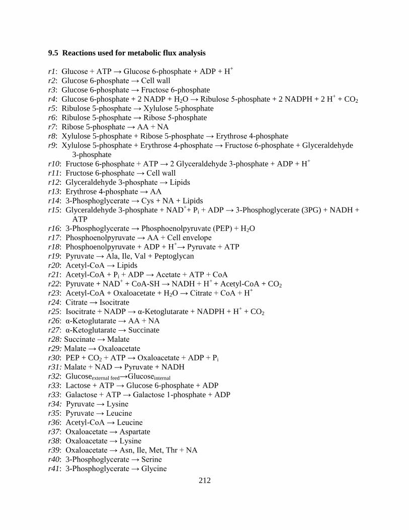
212
9.5 Reactions used for metabolic flux analysis
r1: Glucose + ATP → Glucose 6-phosphate + ADP + H+
r2: Glucose 6-phosphate → Cell wall
r3: Glucose 6-phosphate → Fructose 6-phosphate
r4: Glucose 6-phosphate + 2 NADP + H2O → Ribulose 5-phosphate + 2 NADPH + 2 H+ + CO2
r5: Ribulose 5-phosphate → Xylulose 5-phosphate
r6: Ribulose 5-phosphate → Ribose 5-phosphate
r7: Ribose 5-phosphate → AA + NA
r8: Xylulose 5-phosphate + Ribose 5-phosphate → Erythrose 4-phosphate
r9: Xylulose 5-phosphate + Erythrose 4-phosphate → Fructose 6-phosphate + Glyceraldehyde
3-phosphate
r10: Fructose 6-phosphate + ATP → 2 Glyceraldehyde 3-phosphate + ADP + H+
r11: Fructose 6-phosphate → Cell wall
r12: Glyceraldehyde 3-phosphate → Lipids
r13: Erythrose 4-phosphate → AA
r14: 3-Phosphoglycerate → Cys + NA + Lipids
r15: Glyceraldehyde 3-phosphate + NAD++ Pi + ADP → 3-Phosphoglycerate (3PG) + NADH +
ATP
r16: 3-Phosphoglycerate → Phosphoenolpyruvate (PEP) + H2O
r17: Phosphoenolpyruvate → AA + Cell envelope
r18: Phosphoenolpyruvate + ADP + H+→ Pyruvate + ATP
r19: Pyruvate → Ala, Ile, Val + Peptoglycan
r20: Acetyl-CoA → Lipids
r21: Acetyl-CoA + Pi + ADP → Acetate + ATP + CoA
r22: Pyruvate + NAD+ + CoA-SH → NADH + H
+ + Acetyl-CoA + CO2
r23: Acetyl-CoA + Oxaloacetate + H2O → Citrate + CoA + H+
r24: Citrate → Isocitrate
r25: Isocitrate + NADP → α-Ketoglutarate + NADPH + H+ + CO2
r26: α-Ketoglutarate → AA + NA
r27: α-Ketoglutarate → Succinate
r28: Succinate → Malate
r29: Malate → Oxaloacetate
r30: PEP + CO2 + ATP → Oxaloacetate + ADP + Pi
r31: Malate + NAD → Pyruvate + NADH
r32: Glucoseexternal feed→Glucoseinternal
r33: Lactose + ATP → Glucose 6-phosphate + ADP
r33: Galactose + ATP → Galactose 1-phosphate + ADP
r34: Pyruvate → Lysine
r35: Pyruvate → Leucine
r36: Acetyl-CoA → Leucine
r37: Oxaloacetate → Aspartate
r38: Oxaloacetate → Lysine
r39: Oxaloacetate → Asn, Ile, Met, Thr + NA
r40: 3-Phosphoglycerate → Serine
r41: 3-Phosphoglycerate → Glycine

213
r42: Glycerol + ATP → Glyceraldehyde 3-phosphate + ADP
r43: Glucoseinternal + ATP → Glycogen + ADP
9.6 Calculation of rho values for accumulation vector in MFA
The rho_10% and rho5% columns contains calculations based on a 10% or 5% production of
target protein (from total protein pool), respectively.
r precursor component number rho_P rho_c_p rho_c rho_10% rho_5%
8 R5P x17 0.365 0.144 0.753 0.9195 0.90845
14 E4P x18 1.003 0.361 0 0.4252 0.3931
18 PEP x19 1.869 0.668 0.051 0.8392 0.77915
19 Pyruvate x20 4.236 2.75 0.083 2.9814 2.9071
20 AcCoA x21 0.82 0.428 2.5 2.967 2.9474
26 KG x23 1.663 0.991 0.087 1.1447 1.1111
28 OA x24 2.905 1.447 0.339 1.9322 1.8593
15 3PG x25 1.275 0.874 0.616 1.5305 1.51045
13 Glyc3P x26 0 0 0.129 0.129 0.129
12 F6P x27 0 0 0.071 0.0709 0.0709
3 G6P x28 0 0 0.205 0.205 0.205

214
9.7 MATLAB code for dynamic modeling
function [leastsqdiff, T,Y]=dynamic12hrindlactose(thekvalues,Tstar,Ystar2)
%Tstar=xlsread('expdata.xlsx','12hrindlactose','A1:A5') %Ystar=xlsread('expdata.xlsx', '12hrindlactose','B1:G5') %k=[0.5; 0.5; 3; 1; 2]';fminsearch(@(k) mfile(k,Tstar,Ystar2),k)
%constants constant(1) = 0.2; %1/h constant(2) = 500; %g/L substrate concentration in feed constant(3) = 5; %cell mass at time of feed constant(4)= 1.05; %volume at time of feed constant(5)= 1; %oxygen used for glucose oxidation constant(6) = 0.15; %g/gh, acetate reutilization constant(7) = 1.3; %maximum uptake of glucose
constant(8)= 0.04; %maintenance constant(9) = 0.04; %mol C/g carbon content in mol/g cell constant(10) = 1/30; %mol C/g carbon content per gram of glucose constant(11) = 1.067; %yield of acetate from oxygen constant(12) = 0.667; %g/g yield of acetate on glucose constant(13) = 0.15; %g/g yield of overflow cells on glucose constant(14) = 0.5; %g/g yield of cells from glucose constant(15)= 1.067; %yield of glucose from oxygen constant(16)= 0.51; %aerobic yield coefficient constant(17)= 0.4; %yield of cells from acetate constant(18)= 1.1; %g/g cell/oxygen constant(19) = 10; %amount of lactose added constant(20)= 1; %maximum uptake of lactose
%variables %thekvalues(1)= 1.5066; %g/L fit to %thekvalues(2)= 1.075; %g/L saturation constant for acetate %thekvalues(3)= .95; %g/L fit to data – eventually
%thekvalues(4)= 0; %g/l saturation constant for lactose %thekvalues(5)= 8.5915; %the exponent on the qAg term
initialconditions = [0.00 1.05 5.0 0 10.0 0]; ODESolverOptions = odeset('NonNegative',[1 2 3 4 5 6]);
% First integrate system whilst there is no feed from zero to seven hours % [T,Y]=ode23(@dynamicmodel,[0 7], initialconditions, ODESolverOptions);
% simulation data
[T,Y]=ode15s(@dynamicmodel,[0 7], initialconditions, ODESolverOptions); mn=size(Y); C1=0.006; C2=Y(mn(1),2); C3=Y(mn(1),3); C4=Y(mn(1),4); C5=Y(mn(1),5); C6=Y(mn(1),6); initialconditions2 = [C1 C2 C3 C4 C5 C6]; mn=length(T);
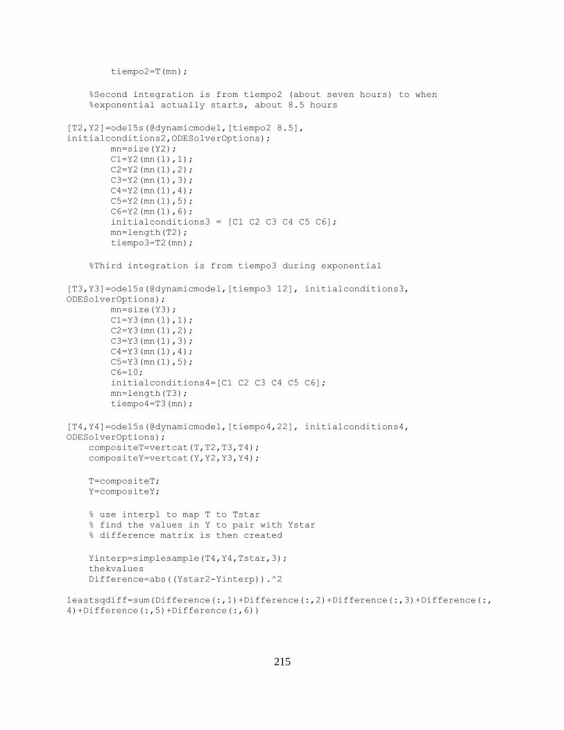
215
tiempo2=T(mn);
%Second integration is from tiempo2 (about seven hours) to when %exponential actually starts, about 8.5 hours
[T2,Y2]=ode15s(@dynamicmodel,[tiempo2 8.5],
initialconditions2,ODESolverOptions); mn=size(Y2); C1=Y2(mn(1),1); C2=Y2(mn(1),2); C3=Y2(mn(1),3); C4=Y2(mn(1),4); C5=Y2(mn(1),5); C6=Y2(mn(1),6); initialconditions3 = [C1 C2 C3 C4 C5 C6]; mn=length(T2); tiempo3=T2(mn);
%Third integration is from tiempo3 during exponential
[T3,Y3]=ode15s(@dynamicmodel,[tiempo3 12], initialconditions3,
ODESolverOptions); mn=size(Y3); C1=Y3(mn(1),1); C2=Y3(mn(1),2); C3=Y3(mn(1),3); C4=Y3(mn(1),4); C5=Y3(mn(1),5); C6=10; initialconditions4=[C1 C2 C3 C4 C5 C6]; mn=length(T3); tiempo4=T3(mn);
[T4,Y4]=ode15s(@dynamicmodel,[tiempo4,22], initialconditions4,
ODESolverOptions); compositeT=vertcat(T,T2,T3,T4); compositeY=vertcat(Y,Y2,Y3,Y4);
T=compositeT; Y=compositeY;
% use interpl to map T to Tstar % find the values in Y to pair with Ystar % difference matrix is then created
Yinterp=simplesample(T4,Y4,Tstar,3); thekvalues Difference=abs((Ystar2-Yinterp)).^2
leastsqdiff=sum(Difference(:,1)+Difference(:,2)+Difference(:,3)+Difference(:,
4)+Difference(:,5)+Difference(:,6))

216
function dy = dynamicmodel(t,y); dy = zeros(6,1); % a column vector
%Feed equation if t<8.5 dy(1)=0; else dy(1)=0.19*y(1) end
%Volume equation dy(2)=y(1);
%Biomass equation dy(3)=(.125-y(1)/y(2))*y(3);
%Acetate equations if t<8.5 dy(4)=0 else qAg=(y(5)/(y(5)+thekvalues(2)))^thekvalues(5); qAc=constant(6)*(y(4)/(y(4)+thekvalues(2))); dy(4)=0.05*y(3)-qAc*y(3)-(y(1)/y(2))*y(4); end
%Glucose equation; thekvalues3 = uptake of glucose when acetate is
present; thekvalues1 = saturation constant for glucose
dy(5)=(y(1)/y(2))*(constant(2)-y(5))-y(5)/(y(5)+thekvalues(1)))*y(3);
%lactose equation if t<12 dy(6)=0; else
dy(6)=y(1)/y(2)*(constant(19)-y(6))-
(constant(20)/(1+(y(6)/thekvalues(4))))*
(y(5)/(y(5)+thekvalues(4)))*y(3); end
end end
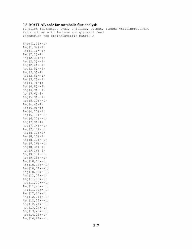
217
9.8 MATLAB code for metabolic flux analysis function [objrates, fval, exitflag, output, lambda]=mfalinprogshort %autoinduced with lactose and glycerol feed %construct the stoichiometric matrix A
%Aeq(1,31)=1; Aeq(1,32)=1; Aeq(1,1)=-1; Aeq(2,1)=1; Aeq(2,32)=1; Aeq(2,3)=-1; Aeq(2,4)=-1; Aeq(2,5)=-1; Aeq(3,5)=1; Aeq(3,6)=-1; Aeq(3,7)=-1; Aeq(4,7)=1; Aeq(4,8)=-1; Aeq(4,9)=-1; Aeq(5,6)=1; Aeq(5,9)=-1; Aeq(5,10)=-1; Aeq(6,4)=1; Aeq(6,9)=1; Aeq(6,10)=1; Aeq(6,11)=-1; Aeq(6,12)=-1; Aeq(7,9)=1; Aeq(7,14)=-1; Aeq(7,10)=-1; Aeq(8,11)=2; Aeq(8,10)=1; Aeq(8,13)=-1; Aeq(8,16)=-1; Aeq(8,34)=1; Aeq(9,16)=1; Aeq(9,17)=-1; Aeq(9,15)=-1; Aeq(10,17)=1; Aeq(10,18)=-1; Aeq(10,31)=-1; Aeq(10,19)=-1; Aeq(11,31)=1; Aeq(11,19)=1; Aeq(11,20)=-1; Aeq(11,23)=-1; Aeq(11,30)=-1; Aeq(12,23)=1; Aeq(12,21)=-1; Aeq(12,22)=-1; Aeq(12,24)=-1; Aeq(13,24)=1; Aeq(13,25)=-1; Aeq(14,25)=1; Aeq(14,26)=-1;

218
Aeq(15,26)=1; Aeq(15,27)=-1; Aeq(15,28)=-1; Aeq(16,28)=1; Aeq(16,30)=1; Aeq(16,24)=-1; Aeq(16,29)=-1; Aeq(17,8)=1; Aeq(18,14)=1; Aeq(19,18)=1; Aeq(20,20)=1; Aeq(21,21)=1; Aeq(22,22)=1; Aeq(23,27)=1; Aeq(24,29)=1; Aeq(25,15)=1; Aeq(26,13)=1; Aeq(27,12)=1; Aeq(28,3)=1; Aeq(31,32)=2; %Aeq(32,31)=1; Aeq(33,5)=2; Aeq(33,26)=1;
%for glycerol feed Aeq(34,34)=1;
%Information for accumulation vector, X %calculation of rho values are based on TP mass 10% of total protein mass
D = 0.13; %Cglucose = 46.1; %Cacetate = 53.12; %Clactose = 6.1; %Caa = 0; biox = 28.5; rho8 = 0.9195; rho14 = 0.4252; rho18 = 0.8392; rho20 = 2.9814; rho21 = 2.97; rho27 = 1.1447; rho29 = 1.9322; rho15 = 1.5305; rho13 = 0.129; rho12 = 0.0709; rho3 = 0.205; rho_lys_pyr = 0.364; rho_leu_pyr = 0.9344; rho_leu_accoa = 0.4672; rho_lys_oa = 0.364; rho_asp_oa = 0.2671; rho_gly_3pg = 0.5944; rho_ser_3pg = 0.2323;

219
beq(1,1) = 0; beq(2,1) = 0; beq(3,1) = 0; beq(4,1) = 0; beq(5,1) = 0; beq(6,1) = 0; beq(7,1) = 0; beq(8,1) = 0; beq(9,1) = 0; beq(10,1) = 0; beq(11,1) = 0; beq(12,1) = 0; beq(13,1) = 0; beq(14,1) = 0; beq(15,1) = 0; beq(16,1) = 0; beq(17,1) = rho8*D; beq(18,1) = rho14*D; beq(19,1) = rho18*D; beq(20,1) = rho20*D; beq(21,1) = rho21*D; beq(22,1) = 1.09/biox; beq(23,1) = rho27*D; beq(24,1) = rho29*D; beq(25,1) = rho15*D; beq(26,1) = rho13*D; beq(27,1) = rho12*D; beq(28,1) = rho3*D; beq(31,1) = 0.35/biox; beq(32,1) = 0/biox; beq(33,1) = 18*D;
%With glycerol feed add the following: Cglyc =204.4; beq(34,1)=Cglyc*D/biox;
La=length(Aeq) Lb=length(beq)
objective(1)=0; objective(2)=0; objective(3)=1; objective(4)=0; objective(5)=0; objective(6)=0; objective(7)=0; objective(8)=1; objective(9)=0; objective(10)=0; objective(11)=0; objective(12)=1; objective(13)=1; objective(14)=1; objective(15)=1; objective(16)=0;

220
objective(17)=0; objective(18)=1; objective(19)=0; objective(20)=1; objective(21)=1; objective(22)=0; objective(23)=0; objective(24)=0; objective(25)=0; objective(26)=0; objective(27)=1; objective(28)=0; objective(29)=1; objective(30)=0; objective(31)=0; objective(32)=0; objective(33)=0; objective(34)=0;
objective=transpose(objective); objective=-1*objective;
A=[]; b=[]; lb=zeros(41); ub=[];
[objrates,fval,exitflag, output, lambda]=linprog(objective,A,b,Aeq,beq,lb,ub)
9.9 Percent error for simulation versus experimental ratios (yield from ATP versus
biomass). Highlighted cells are those with percent error less than or equal to 20%.
12 hr lac -- 0.2 2.18 0.44 1.05 0.93 3.53 0.88 0.84
5 mM IPTG 0.15 -- 1.57 0.54 0.68 0.56 2.64 0.55 0.48
10 mM IPTG 0.57 0.61 -- 0.82 0.35 0.39 0.45 0.41 0.8
AI w/pulse 0.78 1.21 1.02 -- 2.63 2.46 7.44 2.47 0.18
Lac at feed start 0.56 0.41 0.61 0.73 -- 0.05 1.17 0.18 0.59
AI 0.56 0.2 0.64 0.71 0.15 -- 1.42 0.26 0.68
AI (gly) 0.78 0.48 0.3 0.88 0.65 0.57 -- 0.56 0.83
AI w/pulse (gly) 0.47 0.36 0.67 0.71 0.14 0.02 1.41 -- 0.7
15 g lac (gly) 0.56 0.92 4 0.12 1.59 2.18 6.22 2.00 --
Glu
cose
Gly
cero
l
AI w/pulseLac at feed
startAI
Glycerol
AIAI
w/pulse15 g lac
feed experiment 12 hr lac 5 mM IPTG 10 mM IPTG
Top Related