Download - Estimation of Green-Ampt effective hydraulic conductivity

J. Range Manage.

50290-299

Estimation of Green-Ampt effective hydraulic conductivity

for rangelands

MARY R.KTOWELL, MARK A. WELTZ, AND D. PHILLIP GUERTIN

Authors are research assistant and hydrologist. USDA-ARS, Southwest Watershed Research Center. 2000 £ Allen Road. Tucson. Ariz. 85719; associate pro

fessor. School ofRenewable Natural Resources, University ofAriz,. Tucson, Ariz. 85721.

Abstract

Effective hydraulic conductivity (Kg) is an important parame

ter for the prediction of infiltration and runoff volume from

storms. The Water Erosion Prediction Project (WEPP) model,

which uses a modified Green-Ampt equation, is sensitive to the

hydraulic conductivity parameter in the prediction of runoff vol

ume and peak discharge. Two sets of algorithms developed from

cropland data to predict Kg have previsouly been used in the

WEPP model. When tested with data collected on rangelands,

these equations resulted in low predictions of Kg which signifi

cantly over-estimated runoff volume. The errors in runoff pre

diction were propagated through the model and resulted in poor

predictions of peak discharge and sediment yield. The objective

of this research was to develop a new predictive equation to cal

culate Kg specifically for use on rangelands using field data col

lected in 8 western states on 15 different sou/vegetation complex

es. A distinction was made between ground cover parameters

located outside and underneath plant canopy in an effort to

account for the significant spatial variability that occurs on most

rangelands. Optimized Ke values were determined using the

WEPP model and observed runoff data. A regression model

(r*-0.60) was then developed to predict Ke using measured soil,canopy cover, and spatially distributed ground cover data from

44 plots. Independent rangeland data sets are now required to

test the new equation to determine how well the relationships

developed from the data used in this study extend to other range-

land aTftSi

Key Words: WEPP, infiltration, runoff, bydrologic modeling,

spatial variability, ground cover

The Water Erosion Prediction Project (WEPP) model (Lane

and Nearing 1989) was developed to provide process-based ero

sion prediction technology for croplands, rangelands, and forests

to organizations involved in soil and water conservation and envi

ronmental assessment To be successful in predicting erosion, the

model must first succeed in predicting infiltration and surface

runoff. The infiltration component of the WEPP model uses the

Green-Ampt equation (Green and Ampt 1911) as modified by

Ute authors would like to thank all the members of the rangeland study team

who collected the data used in this study including Leonard Lane, Jeff Stone,

Roger Simanura, Mariano Hernandez, Howard Larson, and the many other USDA-

ARS statTand students involved in the project

Manuscript accepted 12 May 1996.

Mein and Larson (1973) to obtain the time to ponding and infil

tration rates for steady rainfall. This equation was further modi

fied by Chu (1978) to simulate infiltration for unsteady rainfall

events, allowing for alternating periods of ponded and impended

conditions.

Although this latest technology for modeling runoff and ero

sion represents* major improvement over older models, signifi

cant problems still exist as a result of the techniques used to esti

mate model parameters under rangeland conditions. This is par

ticularly true in modeling infiltration. Estimates of hydraulic con

ductivity change with the scale of measurement as a result of the

high spatial and temporal variability that exists in natural systems

(Dunne et al. 1991). Current methods for measuring hydraulic

properties in the field are expensive and time consuming and

therefore alternative techniques are needed to estimate model

parameters and improve model results for rangelands.

The approach used in WEPP to simplify parameterization is to

estimate hydraulic properties by relating them to soil and vegeta

tion data that are commonly collected and readily available. The

objectives of this research are to evaluate 2 existing sets of algo

rithms used in the WEPP model to predict effective hydraulic

conductivity (Kg) and to develop an alternative method. All 3

methods are compared to optimized Kg parameters determined

with the WEPP model.

Infiltration Model Description

Green-Ampt Equation

The form of the Green-Ampt equation used in WEPP to calcu

late the infiltration rate after ponding occurs is:

where f is the infiltration rate (mm hr"1), Kg is effective saturated

hydraulic conductivity (m sec"1), Ns is the effective capillary

pressure head at the wetting front (m), and F is the cumulative

infiltration depth (m). Cumulative infiltration depth is calculated

as:

(2)

where t is time (sec) and tp is time to ponding (sec). Effective

capillary pressure head at the wetting front is:

Ns ~ Gle ■ ev) (V - ho) (3)where T|e is field-saturated porosity (tn3 m3), 8V is initial volu-

290 JOURNAL OF RANGE MANAGEMENT 50(3), May 1997

metric water content (m3 m'3), \|/ is the average capillary pressure

head across the wetting front (m), and hg is the depth of ponding

over the soil surface. The average capillary pressure head is esti

mated internally in WEPP as a function of soil properties (Rawls

and Brakensiek 1983).

Prior to surface ponding the infiltration rate is equal to the rain

fall rate and cumulative infiltration is equal to cumulative rain

fall. The infiltration rate starts to decline when ponding begins,

decreasing as the depth of wetted soil increases. If rainfall contin

ues for a sufficient period, infiltration generally approaches a

final, constant, steady rate.

For this study, volumetric water content was calculated as:

ev = wpbpw' (4)

where w is initial soil water content by weight (g g1), pb is drybulk density (gm cm'3), and pw is the density of water (about 1

gm cm'3). Effective field-saturated porosity was calculated as:

ne = 0.9(1- pbpsl) (5)

where ps is soil particle density, and is typically 2.65 gm cm'3 for

a mineral soil.

Parameter Estimation

The importance of hydraulic conductivity in the calculation of

infiltration with the Green-Ampt equation has been well docu

mented. Brakensiek and Onstad (1977) found that the effective

conductivity parameters have a major influence on infiltration

and runoff amounts and rates. Moore (1981) showed that both the

rate and amount of infiltration are more sensitive to hydraulic

conductivity and available porosity than to the wetting front cap

illary potential. Tiscareno-Lopez et al. (1993) concluded that both

the runoff volume and peak runoff rate computed by the WEPP

model are very sensitive to the hydraulic conductivity parameters

in the Green-Ampt equation.

One approach to estimating Green-Ampt hydraulic conductivi

ty is to use an average or effective value, thus ignoring the vari

able and random nature of the physical processes. Green-Ampt

effective hydraulic conductivity (Kg) is a lumped parameter that

integrates a soil's ability to infiltrate water under variable soil

pore structure, surface microtopography, and rainfall amount and

intensity distributions. The Kg value derived in this study pro

vides a single integrated value to represent an entire plot.

Most research to date has focused on saturated hydraulic con

ductivity (Kg), the ability of a soil to transmit water under fully

saturated conditions (Klute and Dirksen 1986), rather than Kg,

because it is comparatively easy to measure under laboratory and

field conditions. One approach consists of correlating hydraulic

conductivity with easily measurable soil properties such as soil

texture, effective porosity, bulk density, and coarse fragments in

the soil.

Rawls and Brakensiek (1989) evaluated a number of physical

factors that are important in the estimation of Kg. Their findings

were incorporated in the algorithms used to calculate Kg in early

versions of WEPP (Rawls et al. 1989). This was accomplished by

adjusting Kg to account for the weight of coarse rock fragments

in the soil, frozen soil, soil crusting, soil macroporosity, and soil

cover, using the following equation:

Ke = Kb [Cf[«BcAcx) Cr) + Mf((\ -Bc)Ac1)) +

(Bo V1) Cr + Mf((l - bJa01)] (6)

where Kb is baseline hydraulic conductivity (m sec'1), Cf is a

canopy correction factor (fraction), Bc is bare area under canopy

(fraction), Ac is total canopy area (fraction), Bo is bare area out

side canopy (fraction), Ao is total area outside canopy (fraction),

Cr is a crust reduction factor (unitless), and Mf is a macroporosity

factor (m ml). Cr is calculated as a function of the average wet

ting front depth, soil crust thickness, a correction factor for partial

saturation of the subcrust soil, and a crust factor. Mf is computed

as a function of sand and clay content. The equations used to cal

culate these variables were developed by Brakensiek and Rawls

(1983) for plowed agricultural soils with a constant crust thick

ness of 0.005m.

Baseline hydraulic conductivity is given by (Rawls et al. 1989):

Kb = Ks(\ -MjFSa (7)

where Kg is saturated hydraulic conductivity (m sec'1), Mcf is the

fraction of course fragments in the soil, and FSa is a frozen soil

factor (unitless). The equation used to calculate Kg was devel

oped from an extensive agricultural soils database (Rawls and

Brakensiek 1985) and is:

Ks = QH(l -Q,)2 (0.001 pt O+) 2 0.00020 C8]"1 (8)

where Qg is effective soil porosity (m3 m'3), Qt is total soil porosity

(m3 m'3), pt is soil bulk density (mg mJ), Or is soil water content

(m3 m'3), and C is an adjustment factor for soil texture (unitless).

The approach outlined above is complex and involves several

levels of nested regression equations. In some cases the parame

ters overlap and thus an error at 1 level can be propagated

through to the final prediction of Kg. Wilcox et al. (1992) report

ed a poor correlation between predicted and observed runoff

using these empirical equations with rangeland data from rainfall

simulation experiments conducted in southwestern Idaho. Savabi

et al. (1995) reported that WEPP underestimated runoff from nat

urally vegetated plots in Texas using the Rawls equation for esti

mating Kg (Eq. 8).

In subsequent versions of the WEPP model, a different set of

algorithms replaced Eq. 6 for predicting Ke. With these algo

rithms, developed by Risse et al. (1995), Kg is calculated directly

from basic soil properties. They are based on WEPP model opti

mization runs of both measured and curve number predicted

runoff quantities on agricultural soils. A number of soil properties

including sand, clay, silt, very fine sand, field capacity, wilting

point, organic matter, CEC, and rock fragments were investigated

through regression analysis to determine which could best be

used in the prediction of Kg.

For soils with a clay content less than or equal to 40%, Kg is

Ke = -0.46 + 0.05 Sai25 + 9.44 CEC0*" (9)

where Sa is percent sand and CEC is the cation exchange capaci

ty (meq/lOOg of soil) in the surface soil layer. If the cation

exchange capacity is less than or equal to 1.0, Ke is:

Ke-8.98 + 0.05 SaIM (10)

If clay content is greater than 40%, Kg is given by:

Ke = -0.016 c1710'' (11)where Cl is percent clay in the surface soil layer.

The combination of equations outlined above resulted in an r2

of 0.78 for the test data set which was comprised of 43 different

soil series. The selected equations were chosen as a result of their

simplicity and the standard error of their estimates.

JOURNAL OF RANGE MANAGEMENT 50(3), May 1997 291

Materials and Methods

Study Sites

Field data collected during the 1987 and 1988 USDA WEPP

rangeland field study from 15 sites with a total of 44 plots in the

Western and Great Plains regions of the United States (Simanton

et al. 1987; 1991) were used for the research described in this

paper. Abiotic and biotic descriptive data for each site are pre

sented in Tables 1 and 2.

Experimental Design and Sampling Methods

Simulated rainfall was applied to undisturbed, paired plots

measuring 3.05 by 10.67 meters using a rotating boom simulator

developed by Swanson (1965). Plots were located in the same

soil and vegetation type at each site. Rainfall simulations were

made on each plot representing dry and wet antecedent moisture

conditions. During the dry run, water was applied at a rate of 60

mm hr'1 for 1 hour. The wet run was made 24 hours later at a rate

of 60 mm hr1 for 30 minutes.

Total rainfall amount and distribution were measured with 6

non-recording raingages positioned around each plot. Rainfall

intensity was measured with a recording raingage located

between the paired plots. Runoff passed through a pre-calibrated

supercritical flume at the downslope end of each plot, flow depths

were measured with a pressure transducer bubble gage, and con

tinuous hydrographs were developed using the flume's depth/dis

charge rating table (Simanton et al. 1987).

A major objective of vegetation data collection was to provide

an estimate of spatial distribution of canopy and ground surface

cover. Measured ground cover characteristics were bare soil, rock

(mineral particles greater than 2 mm), litter (organic material in

direct contact with the soil surface), cryptogams (algae, moss and

lichens), and plant basal cover. Vegetation composition (i.e.

grass, shrub, forb, cactus), canopy cover, ground surface charac

teristics, and surface roughness were measured before rainfall

simulation using a 49-pin point frame placed perpendicular to the

plot slope at 10 evenly spaced transects along the plot border. A

steel pin was lowered vertically at 5 cm intervals along the point

frame. If the pin touched a plant aerial part, the lifeform was

recorded. The pin was then lowered to the plot surface and the

first characteristic touched was recorded for that point for deter

mination of ground cover. It is often difficult to determine where

canopy cover ends and plant basal area begins for areas that have

been heavily grazed, for many prostrate growth form plant types,

and on sites with high surface roughness and pedestaUed plants.

For this work, canopy cover is defined as any plant part elevated

2.5 cm or more from the soil surface. A plant part in contact with

the pinpoint within 2.5 cm of the soil surface is considered to be

basal cover.

Areas located directly underneath plant canopy are referred to

as under-canopy areas while areas located between plants (i.e. no

canopy cover directly above) are referred to as interspace areas

(Fig. la). Total under-canopy ground cover is calculated as the

sum of the fraction of each ground cover component located

under vegetative canopy (as defined above), while total inter

space cover is calculated as the sum of the fraction of each

ground cover component located outside of plant canopy. For

example, if 30% of a plot is covered by rocks, and 40% of those

rocks are in interspace areas while 60% are under-canopy, then

total rock cover in the interspaces is 12% {(40 X 30)/100}.

Similarly, total rock cover under-canopy is 18% {(60 X 30)/100).

Distributions of litter, basal vegetation, and cryptogams are simi

larly calculated. Total interspace and under-canopy area are cal

culated by summing the cover for the individual components

located in their respective areas. Plant nomenclature used

throughout the discussion follows Gould (1975).

Model Configuration and Optimization

Measured topographic, precipitation, vegetation and soils data

from the WEPP rangeland field study were used to run the WEPP

model for a single rainfall event. Topographic data included plot

length, width, and slope values. Measured precipitation data con-

Table 1. Abiotic site characteristics from the WEPP rangeland field experiments.

1)

2)

3)

4)

5)

6)

7)

8)

9)

10)

11)

12)

13)

14)

15)

Site

Tombstone, Ariz.

Tombstone, Ariz.

Susanville, Calif.

SusanviUe, Calif.

Meeker, Colo.

Sidney, Mont.

Los Alamos, N.M.

Cuba. N.M.

Chickasha, Okla,

Chickasha, Okla.

Woodward, Okla.

Freedom. Okla.

Cottonwood. S.Dak.

Cottonwood, S. Dak.

Sonora, Tex.

Soil Family

Usiochreptic calciorthid

Ustollic haplargid

Typic argixeroll

Typic argixeroll

Typic camborthid

Typic argiboroll

Aridic haplustalf

Ustollic camborthid

Udic argiustoll

Udic arguistoll

Typic ustochrept

Typic ustochrept

Typic torrert

Typic torrert

Thermic caldustoll

Soil

series

Stronghold

Forest

Jauriga

Jauriga

Degater

Vida

Hackroy

Querencia

Grant

Grant

Quiftlan

Woodward

Pierre

Pierre

Perves

Surface

texture

Sandy loam

Sandy clay loam

Sandy loam

Sandy loam

Silty clay

Loam

Sandy loam

Sandy loam

Loom

Sandy loam1

Loam

Loam

Clay

Clay

Cobbly clay

Slope

(%)

10

4

13

13

10

10

7

7

5

5

6

6

8

12

8

Elevation

(m)

U77

1.420

1,769

1,769

1.760

N/A

2.144

1,928

378

369

615

553

744

744

650

Vann land abandoned daring the 1930's that had returned to rangeland. The majority of the 'A' horizon had been previously eroded.

292 JOURNAL OF RANGE MANAGEMENT 50(3). May 1997

Table 2. Blotle mean site characteristics from the WEPP rangeland field experiments.

Site Rangeland cover type1Range

site

Ecological

status2 Cover

Standing

Biomass

1) Tombstone, Ariz.

2) Tombstone, Ariz.

3) Susanville, Calif.


5) Meeker, Colo.

6) Sidney, Mont.

7) Los Alamos, N.M.

8) Cuba, N.M.

9) Chickasha, Okla.

10) Chickasha, Okla.

11) Woodward, Okla.

12) Freedom, Okla.

13) Cottonwood, S.Dak.

14) Cottonwood, S.Dak.

15) Sonora, Tex.

Creosotebush-Tarbush

Grama-Tobosa-Shrub

Basin Big Brush

Basin Big Brush

Wyoming bib sagebrush

Wheatgrass-Grama-

Needlegrass

Juniper-Pinyon

Woodland

Blue grama-Calleta

Bkuestem prairie

Bluestem prairie

Bluestem-Grama

Bluestem prairie

Wheatgrass-

Blue grama

Buffalograsse

Juniper-Oak

Limy upland

Loamy upland

Loamy

Loamy

Clayey slopes

Silty

Woodland

community

Loamy

Loamy

prairie

Eroded

prairie

Shallow prairie

Loamy prairie

Clayey west

central

Clayey west

central

Shallow

38

55

55

55

60

58

NA3

47

60

40

28

30

100

30

35

Canopy

32

18

29

18

11

12

16

13

46

14

45

39

46

34

39

Ground

82

40

84

76

42

81

(kg ha1)775

752

5,743

5.743

1483

2,141

72

62

94

70

62

72

68

81

68

1,382

817

2,010

396

1.505

1.223

2,049

529

2,461

'Shiflet(1994).^Ecological status is a similarity index thai expresses the degree to which the composition of the present plant community is a reflection of the historic climax plant community. Thissimilarity index may be used with other site criterion or characteristics to determine rangeland health. Four classes are used to express the percentage of the historic climax plant com

munity on the site: 176-100; IISI-7S; HI 26-50; IV 0-25 (USDA, National Resources Conservation Service (1995).

NA - Ecological status indices are not appropriate for woodland and annual grassland communities.

sisted of rainfall volume, intensity, and duration. Values used to

characterize vegetation included total ground cover by each com

ponent, their distributions between interspace and under-canopy

areas, and total canopy cover. Complete soil pedon descriptions,

sampling, and analysis were made by the USDA-Natural

Resource Conservation Service (NRCS) Soil Survey Laboratory

at each of the rangeland sites as a part of the WEPP Rangeland

Field Study. Measured values of sand, clay, organic matter, bulk

density and cation exchange capacity from the surface horizon

from a single pedon were used. The same values determined from

1 pedon were used to define the soil parameters for all plots at a

particular site.

The rainfall simulation plots were prewet with 60 mm of water

and allowed to drain for 24 hours to minimize antecedent soil

water content differences. Soil water content was measured at 3

locations on the plot: top, middle, and bottom before the rainfall

simulation runs. Soil water content was at or near field capacity

for all sites. Saturation by volume was calculated using the fol

lowing equation (Hillel 1980):

* = 8VV (12)

where s is the degree of saturation by volume, 6V is the volumet

ric water content, and T|e is effective soil porosity.

The WEPP model was used to generate an optimized Kg value

and a corresponding predicted runoff value for each of the 44

plots in the data set under a single storm simulation using data

from the wet run. The model was run for a range of values of Kg

for each plot, and corresponding model predicted runoff volume

was generated. An optimization program, based on a least squares

analysis, was used to interpolate between 2 values of Kg until the

best fit was found.

Data Analysis

Data from the WEPP field studies were used to evaluate Eq. 6

(Rawls et al. i^B9) and Eqs. 9-11 (Risse et al. 1995). Kg valueswere calculated with both equations and compared with the opti

mized Ke values for each plot. The WEPP model was used to

generate runoff volume for both sets of predicted Kg values.

Predicted runoff volume corresponding to each set of predicted

Kg values was then compared with observed runoff volume.

A regression equation was developed and tested using measured

soil and cover data from all of the plots. Maximum r^ regressionanalysis was used to generate regression equations within an 85%

confidence range for the dependent variable (optimized Kg). The

soil parameters included in the analysis were percent sand, silt,

and clay, cation exchange capacity (meq 100 g"1 soil), bulk density

(g cm'1), and organic matter (percent by volume). The components

of ground cover that were evaluated include basal vegetation, litter

(plant residue), rock, and cryptogams. Both the total cover values

JOURNAL OF RANGE MANAGEMENT 50(3). May 1997 293

(a)

Canopy

Caver Area

Canopy

Cower Area

Cryptogam

Uter

Path of nowfng water

(b)

Dobrtt dam ol litter tkwa

the water's velocity and -<

traps scdknenl

Canopy cover Intercepts

ntadrops, reducing their

Mnetfcenergy, therebyreducing sol snaing

vegetation oners the path ofrunoff, slowing its velocity and

" reducing detachment by flowingMRtOf

Uttcf and rocks protect the-

sot) surhco, preventing

raindrop opbrcti detachmentand set teallng

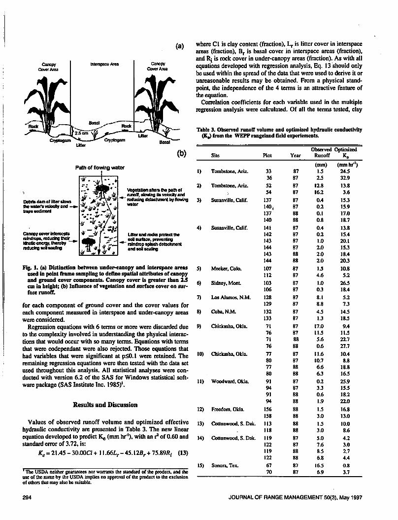
Fig. 1. (a) Distinction between under-canopy and interspace areas

used in point frame sampling to define spatial attributes of canopy

and ground cover components. Canopy cover is greater than 2.5

cm in height; (b) Influence of vegetation and surface cover on sur

face runoff.

for each component of ground cover and the cover values for

each component measured in interspace and under-canopy areas

were considered.

Regression equations with 6 terms or more were discarded due

to the complexity involved in understanding the physical interac

tions that would occur with so many terms. Equations with terms

that were codependant were also rejected. Those equations that

had variables that were significant at pSO.l were retained. The

remaining regression equations were then tested with the data set

used throughout this analysis. All statistical analyses were con

ducted with version 6.2 of the SAS for Windows statistical soft

ware package (SAS Institute Inc. 1985)'.

Results and Discussion

Values of observed runoff volume and optimized effective

hydraulic conductivity are presented in Table 3. The new linear

equation developed to predict Kg (mm hr1), with an r2 of 0.60 and

standard error of 3.72, is:

Ke = 21.45-3O.OOC7 + 11.66Zr-45.12Br+75.89rtl- (13)

' The USDA neither guarantees nor warrants the standard of the product, and theuse of the name by the USDA implies no approval of the product to the exclusion

of others that may also be suitable.

where Cl is clay content (fraction), Lr is litter cover in interspace

areas (fraction), Br is basal cover in interspace areas (fraction),

and Rj is rock cover in under-canopy areas (fraction). As with all

equations developed with regression analysis, Eq. 13 should only

be used within the spread of the data that were used to derive it or

unreasonable results may be obtained. From a physical stand

point, the independence of the 4 terms is an attractive feature of

the equation.

Correlation coefficients for each variable used in the multiple

regression analysis were calculated. Of all the terms tested, clay

Table 3. Observed runoff volume and optimized hydraulic conductivity

(Kf) from the WEPP rangeland field experiements.

Site

Observed Optimized

Plot Year Runoff Ke

1) Tombstone, Ariz.

2) Tombstone, Ariz.



5) Meeker, Colo.

6) Sidney, Mont.

7) Los Alamos, N.M.

8) Cuba, N.M.

9) Chickasha. Okla.

10) Chickasha. Okla.

11) Woodward. Okla.

12) Freedom, Okla.

13) Cottonwood, S. Dak.

14) Cottonwood, S. Dak.

15) Sonora, Tex.

33

36

32

54

137

140,

137

140

141

142

143

144

143

144

107

112

103

106

128

129

132

133

71

76

71

76

77

80

77

80

91

94

91

94

1S6

138

113

118

119

122

119

122

67

70

87

87

87

87

87

87

88

88

87

87

87

87

88

88

87

87

87

87

87

87

87

87

87

87

88

88

87

87

88

88

87

87

88

88

88

88

88

88

87

87

88

88

87

87

(mm)

1.5

2.5

12.8

16.2

0.4

0.2

0.1

0.8

0.4

0.2

1.0

2.0

2.0

2.0

1.5

4.6

1.0

0.3

8.1

8.8

4.5

1.3

17.0

11.5

5.6

0.6

11.6

10.7

6.6

6.3

0.2

3.3

0.6

1.9

1.5

3.0

1.5

3.0

5.0

7.6

8.5

6.8

16.5

6.9

(mm hr'1)24.5

32.9

13.8

3.6

15.3

15.9

17.0

18.7

13.8

15.4

20.1

15.3

18.4

20.3

10.8

5.2

26.5

18.4

5.2

7.3

14.5

18.5

9.4

11.5

2X7

27.7

10.4

8.8

18.8

16.5

25.9

15.5

18.2

22.0

16.8

13.0

10.0

8.6

4.2

3.0

2.7

4.4

0.8

3.7

294 JOURNAL OF RANQE MANAGEMENT 50(3), May 1997

content was shown to have the strongest relationship with Kg

with a moderate negative correlation (R = -0.53) at the 95% sig

nificance level. Conversely, sand content showed a moderate pos

itive correlation (R = 0.48). It has been documented that soil tex

ture is related to hydraulic conductivity on homogeneous soils,

with increased sand content associated with increased conductivi

ty (Rawls et al. 1982). In semiarid watersheds in Nevada,

Blackburn (1975) found a significant relationship between infil

tration rates and soil texture. He reported negative correlations

between clay and silt-sized particles and infiltration, and a posi

tive correlation between sand and infiltration.

Litter cover in interspace areas is represented by a positive term

in Eq. 13, indicating that Kg increases as litter cover in the inter

spaces increases. Litter cover in interspace areas ranged from 2.6

to 61.4% on the 44 plots evaluated, and in general was the most

prevalent ground cover type (Table 4). Litter has long been rec

ognized as effective in reducing soil erosion on rangelands

(Singer et al. 1981, Khan et al. 1988, and Meyer et al. 1970).

Litter cover at the soil surface intercepts raindrops and dissipates

their energy (Fig. 1b). This reduces the clogging of soil pores

with sediment, reducing sealing and crusting, thus enabling more

infiltration. Litter cover also increases potential for debris dam

Table 4. Spatial cover data (%) from the WEPP rangdand field experiments.

1)

2)

3)

4)

5)

6)

7)

8)

9)

10)

11)

12)

13)

14)

15)

Site

Tombstone, Ariz.

Tombstone, Ariz

Susanville. Calif.

Susanville, Calif.

Meeker. Colo.

Sidney, Mont.

Los Alamos, N.M.

Cuba, N.M.

Chickasha.Okla.

Chickasha, Okla.

Woodward, Okla.

Freedom, Okla.

Cottonwood, S.Dak.

Cottonwood, S.Dak.

Sonora, Tex.

Plot

33

36

52

54

137

140

137

140

141

142

143

144

143

144

107

112

103

106

128

129

132

133

71

76

71

76

77

80

77

80

91

94

91

94

1S6

158

113

118

119

122

119

122

67

70

Yr

87

87

87

88

87

88

87

87

87

87

87

88

87

88

87

88

88

88

87

88

87

Total Under-Canopy Cover

Litter

9.2

12.7

5.7

43

24.9

17.6

21.8

18.6

63

9.8

0.0

0.0

6.4

4.1

8.8

5.9

5.1

4.5

7.1

7.3

3.7

4.1

40.6

53.1

20.5

21.0

7.8

8.6

4.8

43

22.2

16.5

23.3

23.3

20.5

19.5

155

21.0

14.7

13.9

13.8

7.6

8.8

26.1

Rock

13.3

13.1

0.0

0.2

1.2

1.2

0.0

0.0

2.4

2.4

0.0

0.0

0.0

0.0

0.0

0.0

0.0

0.2

0.0

0.0

0.0

0.0

0.0

0.0

0.0

0.0

0.0

0.0

0.0

0.0

0.2

0.0

0.0

0.0

0.0

0.0

0.0

0.0

1.2

0.4

0.0

0.0

5.1

1.4

Gyp'

0.0

0.0

0.0

0.0

0.0

0.0

0.0

0.0

0.0

0.0

0.0

0.0

0.0

0.0

0.0

0.0

3.7

5.5

6.5

3.7

5.3

4.1

0.0

0.0

0.0

0.0

0.4

0.2

0.5

0.5

0.0

0.4

1.9

5.2

1.9

1.0

0.0

2.9

0.0

0.0

1.9

0.5

1.0

2.7

Basal

....... t&St. .

0.0

0.0

0.8

2.0

2.0

2.4

6.8

6.4

0.8

0.4

0.0

0.0

4.1

6.8

0.0

0.4

0.6

0.6

0.8

0.6

0.0

0.8

0.8

0.4

18.6

18.6

0.0

0.0

1.4

.Q£

0*

0.6

20.5

19.0

10.0

12.4

19.0

12.4

0.8

0.4

34.3

32.9

0.2

0.8

Litter

7.3

8.1

11.0

13.1

39.2

35.9

35.9

37.3

42.9

45.7

61.8

51.8

27.2

24.1

2.6

22.7

25.1

21.0

12.1

16.4

19.2

17.9

24.9

26.3

50.9

56.1

30.8

25.1

52.8

61.4

13.1

9.0

18.6

26.7

30.5

28.1

27.2

30.0

35.1

37.1

20.0

27.2

11.8

16.3

Total Interspace Cover

Rock

48.7

48.1

3.5

3.1

7.8

15.1

14.5

17.7

19.2

18.0

20.9

23.6

30.9

27.7

0.0

0.0

0.0

0.4

0.6

0.4

0.0

0.0

0.0

0.4

0.0

0.0

0.0

0.0

0.5

0.0

0.2

0.0

0.5

0.0

0.5

0.0

03

1.4

1.2

1.2

2.4

0.5

22.7

1.9

Ciyp

0.0

0.0

0.0

0.0

0.0

0.0

0.0

0.0

0.0

0.0

0.0

0.0

0.0

0.0

0.0

1.2

25.3

38.8

313

25.7

14.3

10.2

0.0

0.0

0.0

0.0

4.3

1.4

4.3

33

2.0

4.9

0.5

10.0

6.7

1.9

0.0

0.4

2.0

0.8

2.9

1.4

5.1

1.2

Basal

2.4

2.2

14.9

19.8

10.2

11.1

4.6

3.6

8.2

4.5

0.0

0.0

1.4

2.7

11.0

11.6

19.0

12.5

15.1

163

20.8

22.9

6.3

17.4

8.5

3.8

15.7

18.3

12.9

203

6.3

6.5

4.3

2.4

6.7

2.4

1.5

5.2

27.0

21.2

93

10.0

16.3

15.5

1 Cryp is cryptogams, defined here as all moss, lichens, and algae.


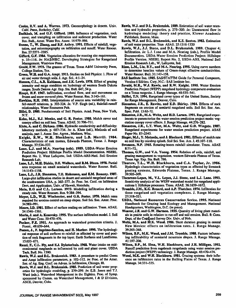
2100

—2000

E

g1&00

a.

■a

11000

5.00

ooo

NaunJnMtU

nog»e

IKMtstmra

•MuatnMia

ScwAMaJ tsMtfl MSO smftr

h rang* condition

StoaJtiad aWUla(«mltr

10 20 30 40 50 60 70 80 S) 100

Basal Cover by Vegetative Growth Form (%)

Fig. 2. Mean annual runoff plotted against basal cover by vegetative

growth form (short grasses and bunch grasses) based on a study

by Hanson et aL (1978). As represented by the dashed line, bunch-

grass and shortgrass basal cover sum to give the total basal cover

for each of the 3 watersheds (low, medium, and high range condi

tions). Also plotted are observed runoff vs. mean total basal cover

from rainfall simulations conducted by the WEPP rangeland

study team (Simanton et aL 1987; 1991) within the low and high

range condition watersheds evaluated by Hanson et aL (1978).

formation, providing an obstacle to the flow of water. The result

is increased tortuosity and hydraulic roughness which reduces

runoff velocity, increasing ponding and infiltration.

Vegetal cover is generally positively correlated to infiltration

and negatively correlated to interrill erosion, whereas bare soil is

generally associated with a decrease in infiltration (Packer 1951,

Dadkhah and Gifford 1980). Many researchers have found higher

infiltration rates under plant canopies than in the interspaces

(Wood and Blackburn 1981, Thurow et al. 1986, and Tremble et

al. 1974). Canopy cover tends to provide protection from rain

drop impact, preventing the formation of a soil crust and dis

lodged soil particles from clogging soil pores, but all plants do

not have the same impact in influencing infiltration rates.

In this study, basal cover in the interspace was found to be neg

atively correlated to Kg and correlation analysis revealed a mod

erate negative relationship between the 2 (R = -0.48). This rela

tionship appears contrary to much of the previous hydrologic

work in which increases in plant cover were related to decreases

in runoff and increases in the apparent infiltration rate. However,

the relation between plant community parameters (e.g., basal

cover) and hydrologic response of uplands is a complex function

that changes depending on the type of plant community being

evaluated. Within a plant community, where the vegetative

growth form remains constant and only the density of plants

changes, the literature consistently indicates that infiltration rate

increases as canopy cover increases (Packer 1951, Dadkhah and

Gifford 1980). When the vegetative growth form shifts (e.g.,

from bunchgrass to shortgrass, or woodland to grassland), the

relationship between basal and canopy cover and infiltration and

runoff appears to shift. That is, equal amounts of vegetative cover

within each of the different plant communities do not necessarily

have the same relationship to apparent infiltration rates and

runoff.

Hanson et al. (1978) initiated a ten-year study of hydrologic

response as a function of grazing intensity at Cottonwood, South

Dakota. They constmcted 4 watersheds (0.9 ha each) in 3 differ

ent pastures representing low, medium, and high range condition

for a total of 12 watersheds. The low condition pasture was domi

nated by shortgrasses such as Bouteloua gracilis (H.B.K.) Lag.

(blue grama) and Buchloe dactyloides (Nutt.) Engelm. (buffalo-

grass). The high condition pasture was dominated by bunchgrass-

es including Agropymn smithii (Rydb.) (western wheatgrass) and

Stipa viridula (Trin.) (green needlegrass). The fair pasture had a

mixture of all 4 grass species. The authors reported that total

annual runoff and runoff from summer convective storms

increased as basal area increased from the bunchgrass-dominated

pasture to the shortgrass-dominated pasture (Pig. 2). Our data

from the Cottonwood research station shows similar results. The

shortgrass-dominated community has a lower apparent infiltra

tion rate than the bunchgrass-dominated site for both years they

were evaluated. All 3 of these watersheds are located on a Pierre

clay soil and no significant differences were found in bulk densi

ty, cation exchange capacity, organic matter, or depth of the A

horizon. The main differences between the sites are in the type of

plant species and the amount of plant biomass present

Other researchers have reported that changes in vegetative

growth form or plant species result in changes in the relationship

between plant attributes of cover and basal area and apparent

infiltration rates and runoff. Thurow et al. (1986) reported that

areas dominated by bunchgrass species had greater infiltration

rates than shortgrass dominated areas in the Edwards Plateau area

in Texas. Rauzi et al. (1968) reported that infiltration rates and

runoff were correlated to plant community type with mid and tall

grass plant communities having higher infiltration rates and lower

runoff rates than shortgrass plant communities using data from

the northern and southern Great Plains regions. Thomas and

Young (1954) found Hilaria mutica (Buckl.) Benth. (tobosa) sites

had higher infiltration rates than did Buchloe dactyloides (Nutt)

Engelm. (buffalograss) sites. Weltz and Wood (1986) reported

that Muhlenbergia richardsonis [Trin.] Rydb. (mat muhly) domi

nated sites had higher infiltration rates than Bouteloua gracilis

(H.B.K.) Lag. (blue grama) dominated sites at Ft. Stanton, N. M.

The plants that dominated the interspaces in this study were

small annual forbs and grasses. The highest total interspace cover

by basal vegetation for any plot in this data set was only 27%,

and most plots had less than 20% cover (Table 4). The exact

mechanism for the reduction of infiltration associated with these

plants is not fully understand. It has been hypothesized that the

reduction in infiltration rate is a function of increased bulk densi

ty, reduced organic matter content of the soil, or the difference in

root distribution and biomass between short, mixed, and tall grass

species. Root biomass in the top 10 cm of the soil was negatively

correlated to Kg in this study (R = -0.47). Short grasses tend to

have a more lateral, matted root structure as compared to the

deeper reaching roots of the mid and tall grasses, resulting in dif

ferences in soil pore structure (Weaver and Harmon 1935). These

differences might affect the ability of water to infiltrate the soil,

resulting in increased runoff from shortgrass dominated sites.

Although root biomass is not a term in Eq. 13, it has a similar

negative relationship to Ke to that of basal area. We hypothesize

that basal cover may be a surrogate for addressing the variability

of soil pore orientation and structure resulting from the lateral

root orientation associated with short grass species.

Blackburn et al. (1992) reported that vegetative growth form

(e.g., shrub, bunchgrass, sodgrass) is one of the primary factors

influencing the spatial and temporal variability of surface soil


processes that control infiltration on rangelands. To improve our

ability to predict infiltration and runoff for these systems, we

must first recognize that they are spatially and temporally influ

enced by growth form, amount, and distribution of native vegeta

tion. Before predictive models can provide realistic estimates of

the influence of alternative land management practices on infil

tration and runoff they must be able to account for vegetation-

induced spatial and temporal variability of soil surface factors. To

accomplish this, new techniques are needed to develop better

infiltration equations and parameters that address the inherent

variability that exists on native and managed rangeland ecosys

tems, and additional research is required to develop a better

understanding of the relationship between plant species and the

infiltration process.

Cooke and Warren (1973) proposed that in a semiarid environ

ment, as vegetal cover decreases, if rocks are present in the soil,

rock cover should increase as a result of the removal of fine parti

cles by raindrop impact and overland flow, leaving the coarse

particles behind. This relationship is seen in the data in this study.

Correlation analysis revealed a moderate negative relationship

between basal cover and rock cover (R = -0.S7). The negative

relationship found between basal cover in the interspaces and Kg

could, therefore, be a secondary effect of low or no rock cover on

those plots.

Rock cover under plant canopy is also positively related to Kg

in Eq. 13, and correlation analysis revealed a moderate positive

relationship (R = 0.31). Only 13 of the 44 plots had any rock

cover under plant canopy, however, and in most cases the per

centage of such cover was very small (Table 4). Rock cover out

side of plant canopy was present on 30 of the plots, and the per

centage of rock cover on these plots was higher than that under

plant canopy, in general, particularly on the shrub sites.

Interspace rock cover and total rock cover were also positively

correlated to Kg (R = 0.38 for both terms), suggesting that the

location of the cover is less important than the actual absence or

presence of rock cover itself.

The literature on the relationship between rock cover and infil

tration and erosion is contradictory. A number of investigators

have reported a negative relationship between rock cover and

infiltration (Tromble et al. 1974, Abrahams and Parsons 1991,

Brakensiek et al. 1986, Haupt 1967, Wilcox et al. 1988), while

others have found a positive relationship (Lane et al. 1987,

Simanton et al. 1984, Meyer et al. 1970). These contradictory

results could be explained by the position of rock fragments in

relation to the soil surface. In a laboratory rainfall simulator

study, Poesen et al. (1990) concluded that rock fragment position

in top soils greatly affects water infiltration. They found that if

the rock fragments rested on the top soil, water intake increased

and runoff decreased. If the rock fragments were embedded in the

top soil, however, infiltration rates were reduced and runoff gen

eration was increased. Such a theory could help to explain the

positive correlation we found.

The fact that 3 of the model terms in Eq. 13 are ground cover

characteristics and that they represent the distribution of those

characteristics as a percentage of either interspace and under-

canopy area suggests the importance of considering areas under

neath and outside plant canopy independently. In semiarid areas,

infiltration and erosion rates are a complex function of plant, soil,

and storm characteristics (Gifford 1984). Although infiltration is

a soil driven process, vegetation influences are great. Spatial veg

etation characteristics such as root density may act as surrogates

for soil characteristics such as bulk density and organic matter.

Many studies have shown that the spatial distribution and the

amount and type of ground cover are important factors influenc

ing both spatial and temporal variations in infiltration and interrill

erosion rates on rangelands (Blackburn et al. 1992, Dunne et al.

1991, Knight et al. 1984, Thurow et al. 1986). In considering Kg,

intended to evaluate hydraulic conductivity for an entire plot, the

apparent importance of ground cover on its prediction is not sur

prising. Given the variability in microtopography within many of

these plots, the interception of flow by ground cover could have a

potentially large impact on infiltration.

It is important to point out that the new predictive equation was

solved for experimental rainfall events with a constant rainfall

intensity of 60 mm hr1, and therefore a constant Kg was predicted

for each site. In reality, the effective hydraulic conductivity of a

hillslope is a nonlinear function of rainfall intensity, initial soil

water content, and the distribution and quantity of canopy and

ground cover. Lane et al. (1978) reported that significant errors in

estimating runoff are possible if it is assumed that a watershed

contributes runoff uniformly over the entire area when only a

small area within the watershed is actually contributing all of the

runoff. Hawkins (1982) observed that the apparent infiltration

rate is a nonnegative function of rainfall intensity. The apparent

infiltration rate will define the mean area! loss rate only when the

maximum infiltration rate has been defined (i.e., when the rainfall

intensity equals or exceeds the maximum infiltration rate of any

portion of die hillslope or watershed).

The interaction of micro-topography and vegetation on surface

storage capacity is one of the major factors that creates confusion

between rainfall simulator results and data from natural rainfall

induced runoff. For many rangeland areas, rainfall consists of

bursts of high rainfall rates followed by reduced rainfall or brief

periods of no rainfall followed by intense rainfall rates. During the

periods of high intensity rainfall, the surface storage areas over

top and runoff is produced. During periods of lower rainfall inten

sity, water in surface storage areas infiltrates and must be filled

again during the next high rainfall burst. These fluctuations in

rainfall intensities contributes to the phenomenon of apparent

infiltration rate changing as a function of rainfall intensity (Morin

and Kosovsky 1995). In addition, runoff generated in bare inter

space areas does not generally flow long distances down slope

before being intercepted by vegetation clumps where all or part of

the runoff is absorbed depending on the infiltration capacity of the

soil. Rainfall simulators with uniform high intensities mask these

processes. New4psearch with variable intensity rainfall simulators

that can reproduce the natural variability in rainfall intensity are

required before rainfall simulator rainfall/runoff results on plots

can be accurately related to natural hillslope or watershed runoff

responses.

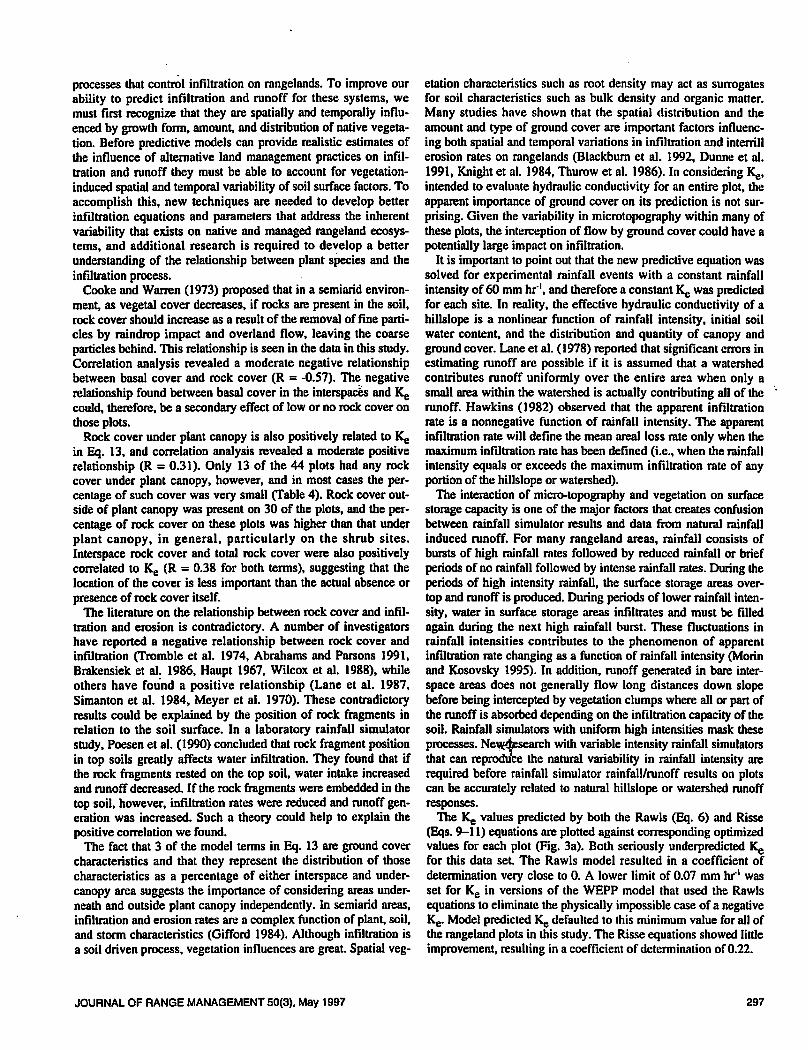
The Kg values predicted by both the Rawls (Eq. 6) and Risse

(Eqs. 9-11) equations are plotted against corresponding optimized

values for each plot (Fig. 3a). Both seriously underpredicted Kg

for this data set. The Rawls model resulted in a coefficient of

determination very close to 0. A lower limit of 0.07 mm hr1 was

set for Kg in versions of the WEPP model that used the Rawls

equations to eliminate the physically impossible case of a negative

Kg. Model predicted Kg defaulted to this minimum value for all of

the rangeland plots in this study. The Risse equations showed little

improvement, resulting in a coefficient of determination of 0.22.

JOURNAL OF RANGE MANAGEMENT 50(3). May 1997 297

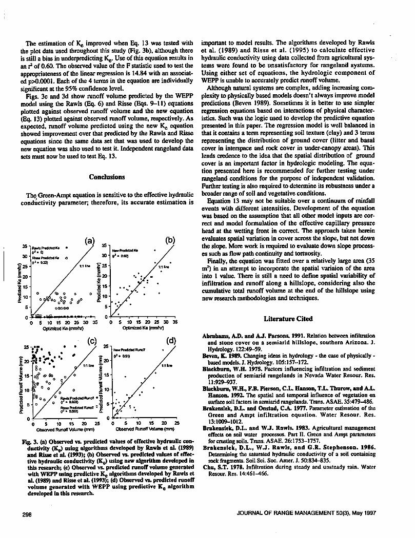
The estimation of Kg improved when Eq. 13 was tested with

the plot data used throughout this study (Fig. 3b), although there

is still a bias in underpredicting Kg. Use of this equation results in

an i2 of 0.60. The observed value of the F statistic used to test the

appropriateness of the linear regression is 14.84 with an associat

ed p>0.0001. Each of the 4 terms in the equation are individually

significant at the 95% confidence level.

Figs. 3c and 3d show runoff volume predicted by the WEPP

model using the Rawls (Eq. 6) and Risse (Eqs. 9-11) equations

plotted against observed runoff volume and the new equation

(Eq. 13) plotted against observed runoff volume, respectively. As

expected, runoff volume predicted using the new Kg equation

showed improvement over that predicted by the Rawls and Risse

equations since the same data set that was used to develop the

new equation was also used to test it. Independent rangeland data

sets must now be used to test Eq. 13.

Conclusions

The Green-Ampt equation is sensitive to the effective hydraulic

conductivity parameter; therefore, its accurate estimation is

35-

30-

25-

20

IS-

10'

5-

fr'-C)

naaPmtctodlto o

(r'-02J)

//

o /^ ° o

7 0 0 0

/ ooooo

(a)

//1:1 Ino

0

35

0 5 10 15 20 25 30 35

Optimized Ke (mnVhr)

5 10 15 20 25 30 35

Optimized Ke (imVtv)

25n

0 5 10 15 20 25

Observed Runoff Volume (mm)

0 5 10 15 20 25

Observed Runoff Vbtume (mm)

Fig. 3. (a) Observed vs. predicted values of effective hydraulic con

ductivity (Kg) using algorithms developed by Rawls et aL (1989)

and Risse et aL (1993); (b) Observed vs. predicted values of effec

tive hydraulic conductivity (Kg) using new algorithm developed in

this research; (c) Observed vs. predicted runoff volume generated

with WEPP using predictive Ke algorithms developed by Rawls et

aL (1989) and Risse et aL (1993); (d) Observed vs. predicted runoff

volume generated with WEPP using predictive Ke algorithm

developed in this research.

important to model results. The algorithms developed by Rawls

et al. (1989) and Risse et al. (1995) to calculate effective

hydraulic conductivity using data collected from agricultural sys

tems were found to be unsatisfactory for rangeland systems.

Using either set of equations, the hydrologic component of

WEPP is unable to accurately predict runoff volume.

Although natural systems are complex, adding increasing com

plexity to physically based models doesn't always improve model

predictions (Beven 1989). Sometimes it is better to use simpler

regression equations based on interactions of physical character

istics. Such was the logic used to develop the predictive equation

presented in this paper. The regression model is well balanced in

that it contains a term representing soil texture (clay) and 3 terms

representing the distribution of ground cover (litter and basal

cover in interspace and rock cover in under-canopy areas). This

lends credence to the idea that the spatial distribution of ground

cover is an important factor in hydrologic modeling. The equa

tion presented here is recommended for further testing under

rangeland conditions for the purpose of independent validation.

Further testing is also required to determine its robustness under a

broader range of soil and vegetative conditions.

Equation 13 may not be suitable over a continuum of rainfall

events with different intensities. Development of the equation

was based on the assumption that all other model inputs are cor

rect and model formulation of the effective capillary pressure

head at the wetting front in correct. The approach taken herein

evaluates spatial variation in cover across the slope, but not down

the slope. More work is required to evaluate down slope process

es such as flow path continuity and tortuosity.

Finally, the equation was fitted over a relatively large area (35

m2) in an attempt to incorporate the spatial variaion of the area

into 1 value. There is still a need to define spatial variability of

infiltration and runoff along a hillslope, considering also the

cumulative total runoff volume at the end of the hillslope using

new research methodologies and techniques.

Literature Cited

Abrahams, A.D. and AJ. Parsons. 1991. Relation between infiltration

and stone cover on a semiarid hillslope, southern Arizona. J.

Hydrology. 122:49-59.

Beven, K. 1989. Changing ideas in hydrology - the case of physically -

based models. J. Hydrology. 105:157-172.

Blackburn, W.H. 1975. Factors influencing infiltration and sediment

production of semiarid rangelands in Nevada Water Resour. Res.

11:929-937.

Blackburn, W.H., F.B. Pierson, C.L. Hanson, T.L. Thurow, and AX.

Hanson. 1992. The spatial and temporal influence of vegetation on

surface soil factors in semiarid rangelands. Trans. ASAE. 35:479-486.

Brakensiek, D.L. and Onstad, C.A. 1977. Parameter estimation of the

Green and Ampt infiltration equation. Water Resour. Res.

13:1009-1012.

Brakensiek, D.L. and WJ. Rawls. 1983. Agricultural management

effects on soil water processes. Part II. Green and Ampt parameters

for crusting soils. Trans. ASAE. 26:1753-1757.

Brakensiek, D.L., W.J. Rawls, and G.R. Stephenson. 1986.

Determining the saturated hydraulic conductivity of a soil containing

rock fragments. Soil Sci. Soc. Amer. J. 50:834-835.

Chu, S.T. 1978. Infiltration during steady and unsteady rain. Water

Resour. Res. 14:461-466.


Cooke, R.V. and A. Warren. 1973. Geomorphology in deserts. Univ.

Calif. Press, Berkeley, Calif.

Dadkhah, M. and G.F. Gifford. 1980. Influence of vegetation, rock

cover, and trampling on infiltration and sediment production. Water

Res. Bull., Amer. Water Res. Assoc. 16:979-986.

Dunne, T., W. Zhang, and B.F. Aubry. 1991. Effects of rainfall, vege

tation, and microtopography on infiltration and runoff. Water Resour.

Res. 27:2271-2285.

Gilford, G.F. 1984. Vegetation allocation for meeting site requirements,

p. 35—116. In: NAS/NRC. Developing Strategies for Rangeland

Management Westview Press.

Gould, F.W. 1975. The grasses of Texas. Texas A&M University Press,

College Station, Tex.

Green, W.H. and &A. Ampt. 1911. Studies on Soil Physics: 1. Flow of

air and water through soils. J. Agr. ScL. 4:1-24.

Hanson, C.L., AJL Kuhlman, and J.K. Lewis. 1978. Effect of grazing

intensity and range condition on hydrology of western South Dakota

ranges. South Dakota Agr. Exp. Sta. Bull. 647,54 p.

Haupt, H.F. 1967. Infiltration, overland flow, and soil movement on

frozen and snow-covered plots. Water Resour. Res. 3:145-161.

Hawkins, R.H. 1982. Interpretations of source area variability in rain

fall-runoff relations, p. 303-324. In: V.P. Singh (ed.). Rainfall-runoff

relationships. Water Resources Pub.

HilleL D. 1980. Fundamentals of Soil Physics. Acad. Press, New York,

N.Y. -

Kahn, MJ., EJ. Monke, and G. R. Foster. 1988. Mulch cover and

canopy effect on soil loss. Trans. ASAE. 31:706-711.

Khite, A. and C. Dirksen. 1986. Hydraulic conductivity and diffusivity:

labortory methods, p. 687-734. In: A. Klute (ed.). Methods of soil

analysis, part 1. Amer. Soc. Agron., Madison, Wise.

Knight, R.W., W.H. Blackburn, and L.B. Merrill. 1984.

Characteristics of oak moltes, Edwards Plateau, Texas. J. Range

Manage. 37:534-537.

Lane, LJ. and M.A. Nearing (eds). 1989. USDA-Water Erosion

Prediction Project: Hillslope Profile Model Documentation. NSERL

Report No. 2. West Lafayette, Ind: USDA-ARS-Natl. Soil Erosion

Research Lab.

Lane, LJ, M.H. Diskin, D.E. Wallace, and R.M. Dixon. 1978. Partial

area response on small semiarid watersheds. Water Resour. Bull.

14:1143-1158.

Lane, LJn JJL Sinranton, T.E. Hakonson, and EM. Romney. 1987.

Large-plot infiltration studies in desert and semiarid rangeland areas of

the southwestern USA, p. 365-377. In: Proc. InL Conf. on Infiltration

DevL and Application. Univ. of Hawaii, Honolulu.

Mein, R.G and C.L. Larson. 1973. Modeling infiltration during a

steady rain. Water Resourc. Res. 9:384-394.

Meyer, LJ), W.H. Wischmeler, and G.R. Foster. 1970. Mulch rates

required for erosion control on steep slopes. Soil ScL Soc. Amer. Proc.

34:982-991.

Moore, ID. 1981. Effect of surface sealing on infiltration. Trans. ASAE.

24:1546-1561.

Morin, J. and A. Kosovsky. 1995. The surface infiltration model. J. Soil

and Water Cons. 50:470-476.

Packer, P.E. 1951. An approach to watershed protection criteria. J.

Forest.. 49:639-644.

Poesen, J., F. Ingelmo-Sanchez, and H. Mucber. 1990. The hydrologi-

cal response of soil surfaces to rainfall as affected by cover and posi

tion of rock fragments in the top layer. Earth Surfaces and Landforms.

15:653-671.

RauzL F., CX. Fly, and EJ. Dyksterhuis. 1968. Water intake on mid-

continental ranglands as influenced by soil and plant cover. USDA

Tech. Bull. No. 1390.

Rawls, WJ. and D.L. Brakensiek. 1983. A procedure to predict Green

and Ampt infiltration parameters, p. 102-112. In: Proc. of the Amer.

Soc. of Ag. Eng. Conf. on Advan. in Infiltration, Chicago, Dl.

Rawls, WJ. and D.L. Brakensiek. 1985. Prediction of soil water prop

erties for hydrologic modeling, p. 239-299. In: E.B. Jones and T.J.

Ward (eds.). Watershed Management in the Eighties. Proc. of Symp.

sponsored by Comm. on Watershed Management, I & D Division,

ASCE, Denver, Colo.

Rawls, WJ. and D.L. Brakensiek. 1989. Estimation of soil water reten

tion and hydraulic properties, p. 275-300. In: Unsaturated flow in

hydrologic modeling: theory and practice, Kluwer Academic

Publishers, Boston, Mass.

Rawls, WJ. and D.L. Brakensiek, and K.E. Saxton. 1982. Estimation

of soil water properties. Tran ASAE. 25:1316-1320

Rawls, WJ., J.J. Stone, and D.L. Brakensiek. 1989. Chapter 4;

Infiltration. In: L.J. I.nne and M.A. Nearing (eds.). Profile Model

Documention. USDA-Water Erosion Prediction Project: Hillslope

Profile Version. NSERL Report No. 2, USDA-ARS, National Soil

Erosion Research Lab., W, Lafayette, Ind.

Risse, LJVL, Liu, B.Y., and M.A. Nearing. 1995. Using curve numbers

to determine baseline values of Green-Ampt effective conductivities.

Water Resour. Bull. 31:147-158.

SAS Institute Inc. 1985. SAS/STATTM Guide for Personal Computers,

Version 6 Edition. Cnry. N.C.: SAS Institute Inc.

Savabi, M.R., WJ. Rawls, and R.W. Knight. 1995. Water Erosion

Prediction Project (WEPP) rangeland hydrology component evaluation

on a Texas rangesite. J. Range Manage. 48:535-541.

Shiflet, T.N. 1994. Rangeland cover types of the United States, Society

for Range Management, Denver, Colo.

Simanton, J.R., E. Rawitz, and E.D. Shirley. 1984. Effects of rock

fragments on erosion of semiarid rangeland soils. Soil Sci. Soc. Am.

Spec. Publ. 13:65-72.

Simanton, JJL, M.A. Weltz, and H.D. Larsen. 1991. Rangeland exper

iments to parameterize the water erosion prediction project mode: veg

etation canopy cover effects. J. Range Manage. 44:276-282.

Simanton, J.R., L.T. West, M.A. Weltz, and G.D. Wingate. 1987.

Rangeland experiments for water erosion prediction project. ASAE

Paper No. 87-2545.

Singer, MJ., Y. Matsuda, and J. Blackard. 1981. Effects of mulch rate

on soil loss by raindrop splash. Soil Sci. Soc. Am. J. 45:107-110.

Swanson, N.P. 1965. Rotating-boom rainfall simulator. Trans. ASAE

8:71-72..

Thomas, G.W., and V.A. Young. 1954. Relation of soils, rainfall, and

grazing management to vegetation, western Edwards Plateau of Texas.

Texas Agr. Exp. Sta. Bull. 786.

Thurow, T.L., W.H. Blackburn, and C.A. Taylor, Jr. 1986.

Hydrologic characteristics of vegetation types as affected by livestock

grazing systems. Edwards Plateau, Texas. J. Range Manage.

39:505-509.

Tiscareno-Lopez, M., V.L. Lopez, JJ. Stone, and LJ. Lane. 1993.

Sensitivity analysis of the WEPP watershed model for rangeland appli

cations I: Hillslope processes. Trans. ASAE. 36:1659-1672.

Tromble, JJVf., K.G. Renard, and AJ». Thatcher. 1974. Infiltration for

three rangeland soil vegetation complexes. J. Range Manage.

27:318-321.

USDA, National Resources Conservation Sevice. 1995. National

Handbook for Grazing land Ecology and Management. National

Headquarters, Washington, D.C. (in press).

Weaver, J.E. and G.W. Harmon. 1935. Quantity of living plant materi

als in prairie soils, in relation to run-off and soil erosion. Bull. 8: Cons.

DepL of the Coo&and Survey Div. Univ. of Neb.

Weltz, M.A. and M.K. Wood. 1986. Short duration grazing in central

New Mexico: effects on infiltration rales. J. Range Manage.

39:365-368.

Wilcox, B.P., M.K. Wood, and J.M. Tromble. 1988. Factors influenc

ing infiltrability of semiarid mountain slopes. J. Range Manage.

41:197-206.

Wilcox, B.P., M. Sbaa, W.H. Blackburn, and J.H. MUligan. 1992.

Runoff prediction from sagebrush rangelands using water erosion pre

diction project (WEPP) technology. J. Range Manage. 45:470-474.

Wood, MIL and W.H. Blackburn. 1981. Grazing systems: their influ

ence on infiltration rates in the Rolling Plains of Texas. J. Range

Manage. 34:331-335.
