


Languages
Pages
Legal

ESSAYS ON MONETARY POLICY, MONETARY
TRANSMISSION AND INFLATION OF INDONESIA
USING GENERAL EQUILIBRIUM MODEL
Thesis submitted for the degree of
Doctor of Philosophy
at the University of Leicester
by
Akhis Reynold Hutabarat
Department of Economics
University of Leicester
April 2010

ii
To my wife, Diana,
my daughters, Audrey, Sarah and Victoria
and my son, Adrian

iii
So don't throw it all away now. You were sure of yourselves then. It's still a sure thing!
But you need to stick it out, staying with God's plan so you'll be there for
the promised completion.
Hebrews 10:35-36 (The Message)
iv
Abstract
Essays on Monetary Policy, Monetary Transmission and Inflation of Indonesia
using General Equilibrium Model
Akhis Reynold Hutabarat
The first essay attempts to explain how the economy responds to transient exogenous
exchange rate and cost-push shocks using a small open economy New Keynesian
dynamic general equilibrium model that incorporates prices and wage stickiness and
cost channel of interest rate to inflation. The model shows that a low degree of prices
and wage rigidity, high reliance on imports and inflation-biased monetary policy,
increases exchange rate pass-through to domestic and consumer prices. The model
demonstrates that the transient nature of cost-push shock, combined with rational
expectation behaviour of price setter and full policy credibility, does not require the
monetary authority in developing economy to respond to the shock by tightening
monetary policy.
The second essay investigates the relative importance of monetary transmission channel
to inflation of passing persistent shock to the risk premium. The findings show that
nominal exchange rate depreciation, triggered by a more persistent shock to interest risk
premium, worsens the state of the economy in the short- and long-run. Such distinctive
shocks effect is transmitted through the economy that typifies lack of response of
consumer price disinflation to interest rate tightening caused by high real rigidity, strong
cost channel of interest rate, strong cost channel of exchange rate pass-through and
weak demand-side channel of exchange rate pass-through.
The final essay analyses Indonesia‘s inflation determinant using a model that links
banking to real sector, central bank and government. It explores interest rate cost-push
channel in terms of cost of equity and cost of borrowing, enhances the previous findings
about the lack of response of disinflation to interest rate policy tightening and discusses
the nexus between monetary and banking policy. The strong interest rate cost channel
has some implications for the behaviour of and policy for banking related to the
achievement of the inflation target.

v
Acknowledgments
I lift up praise and gratitude to the Lord Jesus for everything in my life is fully under his
consent and control, including this study. I thank you God for sending me to Leicester,
helping me in times of difficulties, providing me with abundant wisdom and
understanding, and eventually opening the doors widely of completing this thesis. May
your name be exalted, honoured and glorified.
This project would not have been possible without the support of many people. I am
heartily thankful to my supervisor, Professor Stephen Hall, who has been exceptionally
kind, patient, optimistic, responsive and resourceful in guiding and supporting me from
the initial phase to the full completion of this thesis. I am also grateful to my supervisor
and the members of the thesis committee, Professor Kevin Lee and Dr. Martin Hoskins,
who offered me challenging insights and superb advice for the direction and progress of
my study.
I would like to convey my thankfulness to Bank Indonesia, particularly the management
and staff of Human Resources Development Directorate and London Representative
Office, for giving me the scholarship as well as providing outstanding assistance and
guidance. I would also like to thank my colleagues at the Directorate of Economic
Research and Monetary Policy and my fellow Bank Indonesia‘s student in the UK for
sharing data and information as well as technical and nontechnical help.
I would like to thank the academic and support staff of the Department of Economics,
Graduate Office, Library and IT services University of Leicester for excellent provision
and arrangement of academic and study life environment. I am thankful to my fellow
PhD student and office mates for their warm attention, encouragement and invaluable
advice. I wish you all good luck with your study and career and have a successful life.
I am grateful to Bob and Mina Coffey, Fiona Hamilton and my fellow home group at
Knighton Evangelical Free Church for their constant prayer, attention, encouragement,
advice and even a one-time worry that stimulated turning point and breakthrough to my
study progress. I extend my thankfulness to Stephanus Mudjiono and Henry Susanto,
and their family, for supporting me and my family through spiritual advice and prayer.
I owe my deepest gratitude and love to my wife, Diana. She deserves utmost special
mention for her remarkable and inseparable support, love and prayers throughout this
journey. I also thank my children, Audrey, Sarah, Adrian and Victoria for bringing me
joy and persistently praying for me. I extend my gratitude to my parent-in-law, Mr. and
Mrs. Sidabutar, and to my sisters, Esther, Ernita and Nora, for keep putting me and my
family into their prayer time slot. I offer my regards and blessings to all of those who
supported me in any respect during the completion of this project.
Last but not least, I am deeply indebted and grateful to my late mother, Elise Rosmin,
who instigated my decision to undertake this study through her visionary suggestion and
supported me with bountiful love and continual prayer throughout her last painful years.
I wish she could have seen me accomplish the job she ‗assigned‘ me to do years ago.
Leicester, 16 April 2010
Akhis Reynold Hutabarat
vi
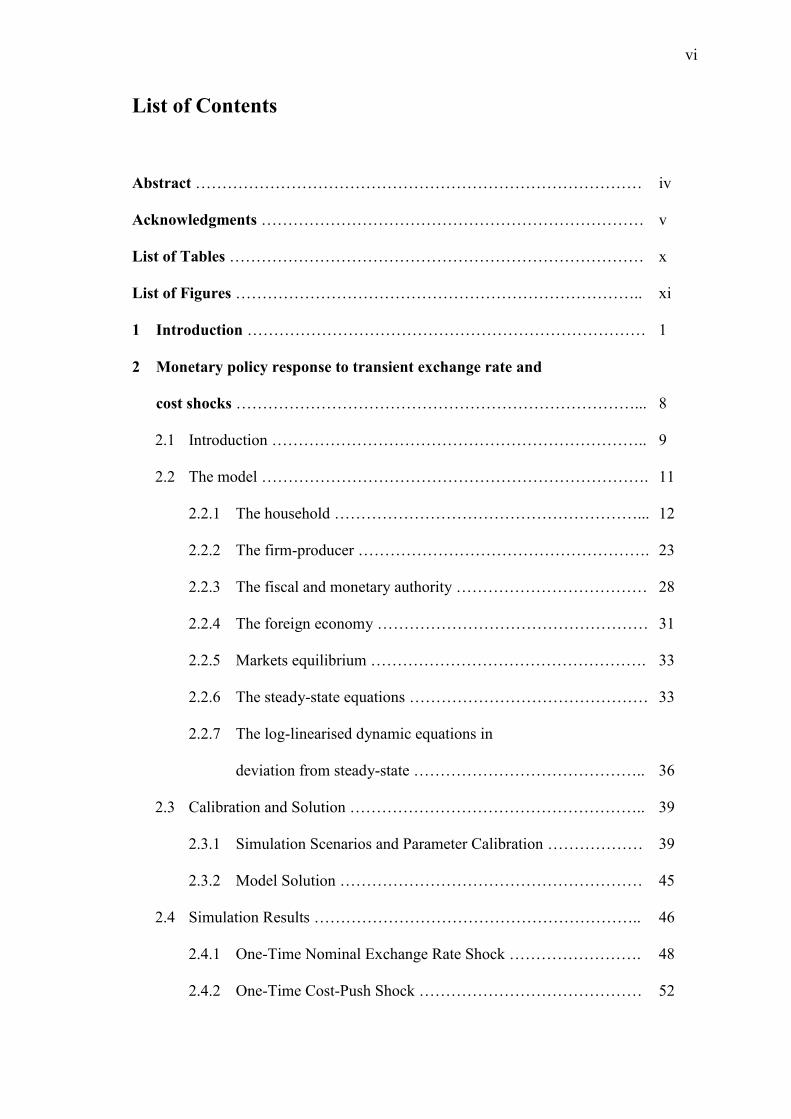
List of Contents
Abstract ………………………………………………………………………… iv
Acknowledgments ……………………………………………………………… v
List of Tables …………………………………………………………………… x
List of Figures ………………………………………………………………….. xi
1 Introduction ………………………………………………………………… 1
2 Monetary policy response to transient exchange rate and
cost shocks …………………………………………………………………... 8
2.1 Introduction …………………………………………………………….. 9
2.2 The model ………………………………………………………………. 11
2.2.1 The household …………………………………………………... 12
2.2.2 The firm-producer ………………………………………………. 23
2.2.3 The fiscal and monetary authority ……………………………… 28
2.2.4 The foreign economy …………………………………………… 31
2.2.5 Markets equilibrium ……………………………………………. 33
2.2.6 The steady-state equations ……………………………………… 33
2.2.7 The log-linearised dynamic equations in
deviation from steady-state …………………………………….. 36
2.3 Calibration and Solution ……………………………………………….. 39
2.3.1 Simulation Scenarios and Parameter Calibration ……………… 39
2.3.2 Model Solution ………………………………………………… 45
2.4 Simulation Results …………………………………………………….. 46
2.4.1 One-Time Nominal Exchange Rate Shock ……………………. 48
2.4.2 One-Time Cost-Push Shock …………………………………… 52
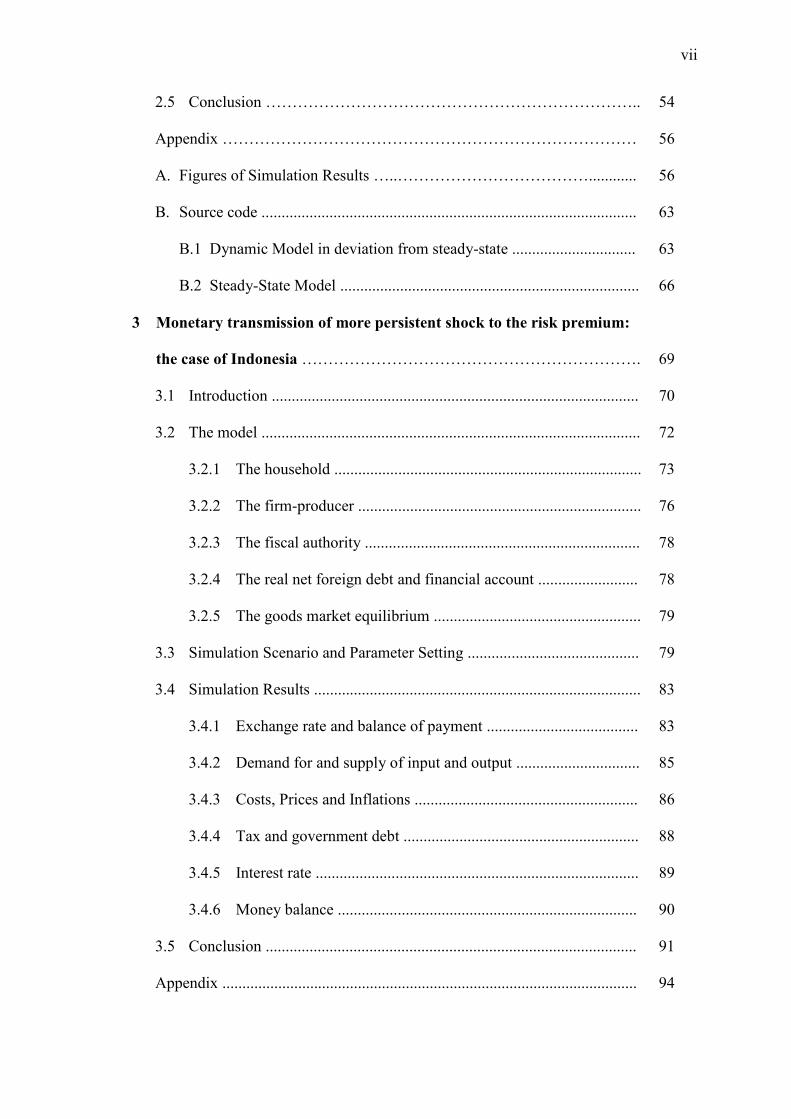
vii
2.5 Conclusion …………………………………………………………….. 54
Appendix …………………………………………………………………… 56
A. Figures of Simulation Results …..………………………………............ 56
B. Source code .............................................................................................. 63
B.1 Dynamic Model in deviation from steady-state ............................... 63
B.2 Steady-State Model ........................................................................... 66
3 Monetary transmission of more persistent shock to the risk premium:
the case of Indonesia ………………………………………………………. 69
3.1 Introduction ............................................................................................ 70
3.2 The model ............................................................................................... 72
3.2.1 The household ............................................................................. 73
3.2.2 The firm-producer ....................................................................... 76
3.2.3 The fiscal authority ..................................................................... 78
3.2.4 The real net foreign debt and financial account ......................... 78
3.2.5 The goods market equilibrium .................................................... 79
3.3 Simulation Scenario and Parameter Setting ........................................... 79
3.4 Simulation Results .................................................................................. 83
3.4.1 Exchange rate and balance of payment ...................................... 83
3.4.2 Demand for and supply of input and output ............................... 85
3.4.3 Costs, Prices and Inflations ........................................................ 86
3.4.4 Tax and government debt ........................................................... 88
3.4.5 Interest rate ................................................................................. 89
3.4.6 Money balance ........................................................................... 90
3.5 Conclusion ............................................................................................. 91
Appendix ........................................................................................................ 94
viii
A. Figures ………………………………………………………………….. 94
B. The steady-state equations ....................................................................... 102
C. The log-linearised dynamic equations in deviation
from steady-state ...................................................................................... 105
D. Source code .............................................................................................. 108
D.1 Dynamic Model in deviation from steady-state ............................... 108
D.2 Steady-State Model ........................................................................... 113
4 Indonesia’s inflation determinant: demand-pull vs. cost-push ................ 115
4.1 Introduction ........................................................................................... 116
4.2 The model .............................................................................................. 119
4.2.1 The firm ...................................................................................... 119
4.2.2 The bank ..................................................................................... 124
4.2.3 The central bank ......................................................................... 133
4.2.4 The government .......................................................................... 137
4.2.5 The household ............................................................................ 139
4.3 Cost push vs. demand pull inflation ...................................................... 143
4.3.1 Cost-push inflation ..................................................................... 145
4.3.2 Demand-pull inflation ................................................................ 147
4.3.3 Demand-pull inflation, GDP, money and output gap ................. 152
4.3.4 Bank‘s interest rate and monetary and banking policy .............. 154
4.4 Steady-State Simulation ......................................................................... 159
4.4.1 An increase in capital adequacy ratio ......................................... 162
4.4.2 A higher required reserve ratio ................................................... 163
4.4.3 A higher tax base ratio ……........................................................ 164
4.4.4 A higher household‘s currency-to-deposit ratio .......................... 165

ix
4.5 Conclusion .............................................................................................. 171
Appendix: Source code ................................................................................... 174
5 Concluding remarks ..................................................................................... 179
References ……………………………………………………………………… 185
x
List of Tables
2.1 Model Calibration ………………………………………………………... 44
3.1 Model Calibration ………………………………………………………... 80
3.2 Correlation between currency growth and interest rate ………………….. 91
4.1 Model Calibration (baseline) …………………………………………….. 159
4.2 Steady State Simulation Results (higher ratio or policy rate) ……………. 166
4.3 Steady State Simulation Results (lower ratio or policy rate) …………….. 168
xi
List of Figures
2.1 Monetary Policy Transmission …………………………………………. 31
2.2 Response Parameters and Welfare Loss (Exchange Rate Shock)……...... 43
2.3 Response Parameters and Welfare Loss (Cost Shock) ……………....….. 43
2.4 Illustration of shock simulation to a real variable ………………………. 47
2.5 Illustration of shock simulation to a nominal variable ………………….. 48
2.6 Short run trade-off between output and inflation
(one-time exchange rate shock) ……………………….............................. 52
2.7 Short run trade-off between output and inflation
(one-time cost shock) ………………………............................................. 53
2.8 Responses to One-Time Nominal Exchange Rate Shock ……………….. 56
2.9 Responses to One-Time Cost-Push Shock ………………………………. 59
3.1 Range of Feasible Response Parameter …………………………………. 94
3.2 Responses to an eight-quarter one percentage point shock
to the risk premium ……………………………………………………… 94
3.3 Real Exports, Real Imports and Trade Surplus of Indonesia …………… 99
3.4 Effect of the optimality of monetary policy response to
risk premium shock ……………………………………………………... 100
3.5 Direction of interest rate and growth of currency in Indonesia …………. 102
4.1 Gross Domestic Income ……………………………………………….... 147
4.2 Consumption of goods and services (steady-state solution) ……………. 149
4.3 Households Non-Loan Goods Consumption Financing
(steady-state solution) …………………………………………………... 150
4.4 Corporate‘s Source of Investment Fund ................................................... 151

xii
4.5 Gross Domestic Product (steady-state solution) ………………………… 152
4.6 Household Consumption ………………………………………………… 154
4.7 Bank‘s Return on Assets ………………………………………………… 159

Chapter 1
Introduction
2
Monetary management needs to establish on a more comprehensive knowledge about
monetary transmission mechanism and the relative strength among monetary channels.
The omission of important channel in the framework of monetary policy formulation
could put the monetary policy makers in a greater risk of making an inappropriate
policy conduct in pursuing their target, particularly the overarching target of inflation.
The interest rate cost channel is a controversial monetary transmission channel that
has not been included in the Bank Indonesia's policy and forecasting system of
modelling. Yet the indication of its significance could have been drawn from the so
called ―price puzzle‖ phenomenon in the bank‘s study about monetary transmission of
bank lending channel (Agung, 2001), as well as from the weak sensitivity of disinflation
to interest rate increases in the bank‘s small macroeconometric model (Majardi, 2004).
The channel has also received trivial awareness in the framework of thinking in
policy decision making within the central bank. Aslim Tadjuddin, the Bank Indonesia‘s
deputy governor in 2002-07, was the prominent critics in the central bank of the
common approach to combat inflation by raising the interest rate. He considered that
there is a positive causality from policy interest rate to inflation due to strong interest
cost channel. He also often raised concern about distinguishing economic environment
differences between Indonesia and advanced economies.
However, there have been a growing research interest about cost channel of interest
rate policy to inflation since early of the last decade (see for instances, Barth and Ramey
2001, Linnemann 2005, Chowdhury et al. 2006, Ravenna & Walsh 2006, Castelnuovo
& Surico (2006), Henzel et al. 2008, Lima and Setterfield 2010). Agénor and Montiel
(2008) noted that the interest rate cost channel has been proposed as an explanation of
the ―price puzzle‖ phenomenon, which was labelled by Eichenbaum (1992) referring to
3
the existence of a positive correlation between increases in the short-term interest rate
and the price level in Sims‘ (1992) empirical anomaly finding.
The issue about the positive effect of interest rate on price or inflation has even
been of the subject of interest for some macroeconomist since the nineteenth century
originated in the work of Thomas Tooke (1838). Smith (2006) summarised Tooke‘s
work in his argument that Thomas Tooke‘s most important legacy to economics was his
original proposition that the long-run ―average‖ rate of interest entered into the normal
cost of production and, therefore, the normal prices of commodities, reflecting the
notion that the interest rate systematically governs the normal rate of profit.
Gibson (1923), in an article for Banker's Magazine, noted that the positive
correlation existed between interest rates and prices in the UK over a period of 200
years. John Maynard Keynes, in his 1930 work, A Treatise on Money, labelled the
correlation as ‗Gibson paradox‘ because the economic theory of the time, the Irving
Fisher‘s theorem, suggested that the interest rate should move with the inflation or the
expected inflation rather than the price level itself.
Seelig (1974) develops the theoretical model that underlies the econometric
analysis to examine the impact of interest rate changes on price changes via mark-up
pricing. His work was a response to the ―Wright Patman effect‖, the more recent name
related to the interest cost-push channel, after the US Congressman‘s view that it is
senseless "to fight inflation by raising interest rates. Throwing gasoline on a fire to put
out the flames would be as logical." The statistical and economic insignificance of his
results does not support the hypothesis that increases in interest rates lead to higher
prices via mark-up pricing during 1950s and 1960s. However, the positive correlation
between interest rate and inflation occurs when interest rates is doubled.

4
Driskill and Sheffrin (1985) examined the disputed relations between interest rates
and prices, by introducing interest costs into John Taylor's model of overlapping wage
contracts. They found that the presence of interest costs does affect the stabilization
process and can make the tradeoffs between output and price variability less favourable.
However, their analysis does not substantiate the view that monetary policy cannot
lower the inflation rate because of the price effects on interest rates.
Another name for the interest rate cost-push channel is the ‗Cavallo-effect‘ after the
Argentine minister of the economy during the 1990s, Domingo Cavallo, who found
empirical support for the channel of the real cost of working capital in his Harvard PhD
thesis (Taylor 2004). S. van Wijnbergen (1981) applied the Cavallo-effect for South
Korea. He developed a quarterly macroeconometric model that had a linkage between
financial and real sector explicitly and incorporated the transmission channel of
monetary policy into the supply side of the economy via the real costs of working
capital. His model simulation showed a strong stagflationary effect of monetary policy
tightening in the short-run. This interest rate cost-push channel is the key insight of the
Structuralist model developed most notably by Lance Taylor in the context of his
criticism of the stabilization program in developing countries (Agénor and Montiel
2008).
I put the interest rate cost channel of monetary policy and its relative importance
compared to other channel of monetary policy into the heart of this study. The rationale
for the choice lays on the fact that Indonesia‘s capital share is greater than its labour
share. According to Input-Output Table 2005, the share of return on equity in value
added is 57%, while the employee‘s salary contributes 31% to the total value added. In
contrast, gross domestic income of the United Kingdom comprises 62% of
compensation of employees and 36% of gross operating surplus (Mahajan, 2006). This
5
structural difference between a developing and an advanced country suggests different
agent behaviour and policy implication between Indonesia and advanced economy.
This study also investigates how the channel works in the existence of transient and
elongated shock to the exchange rate. How monetary policy should responds when
interest rate cost-channel interacts with exchange rate pass-through and other demand
and cost channels, is the ultimate concern of this research. Investigating the monetary
policy response to exchange rate shocks in Indonesia is noteworthy for several reasons.
First, adverse exchange rate shock frequently occurs and it has a high possibility of
recurrence. Second, the economy has experienced severe elongated exchange rate shock
that altered the equilibrium exchange rate and other macroeconomic variables. Third,
macroeconometric modelling found a contractionary effect of depreciation possibly due
to high import contents in production structure. Thus, it is interesting to identify the
direction and extent of exchange rate effect on output and factors driving the effect.
Monetary policy is transmitted to the real sector mainly through the banking
system, particularly in developing economies where financial markets are dominated by
commercial banks. Thus, banking intermediary should have a role in a macroeconomic
model as a significant economic player, and the model should provide linkage between
the financial and real sector. However, there has been little attention paid to putting
financial institution into general equilibrium model and in incorporating financial
friction. When such a model does not incorporate banking, there is only one interest rate
that represents policy rate and all market rates. The Economist magazine (April 3rd
2010) noted that this condition like the convenient fiction of a model of the economy
that is defensible as long as different rates moves in concert. Unfortunately, they do not.
As a reflection on the global financial crisis, Cecchetti et al. (2009) raised the
challenge for macroeconomist to construct macroeconomic models that can create
6
severe financial stress endogenously. For the initial step, it requires the extension of the
current macroeconomic modelling approach that ignored financial intermediaries and
focused on rigidities in goods and labour market. There have been few researches that
encompass a link between financial sector and the real economy. Among such limited
researches are Goodfriend and McCallum (2007), Atta-Mensah and Dib (2008), Curdia
and Woodford (2009) and Gerali et al. (2010). In the third part of this study, I attempted
to contribute to such research needs by designing the linkage between financial and real
sector through consolidated budget and balance sheet constraints for all agents. The
model also links the banking sector to the central bank and government. The study then
investigated how the monetary policy channel works in the presence of banking
intermediary.
This research also aims to gain a more solid analytical economic framework and learn
modelling techniques as tools for policy analysis instead of forecasting purposes. Thus, it is
intended to offer an additional conceptual support for monetary policy decision making at
the central bank of Indonesia. With regard to this objective, I choose to use dynamic general
equilibrium models as tools to conduct shocks simulation in the first two studies. The third
study formulated the financial dynamics general equilibrium model but uses the steady-state
stage of the model to conduct parameter and policy simulations. The models were built on
the framework of Christiano et al. (2005), Smets and Wouters (2003), Erceg and Levin
(2003), Woodford (2003), Murchison (2004) and Freixas and Rochet (2008).
Hamann (2004) offered arguments in favour of using dynamic stochastic general
equilibrium models for policy decisions. First, the model can overcome most of the
limitation of the semi-structural models, i.e there are no market clearing conditions and
the aggregate description of the economy is consistent with different microeconomic
stories. Second, the models define clearly what economic actors do when they and
interact meet in the markets. Third, the outcomes in these models is consistent with
7
explicit constrained optimization problems for each agent and the restrictions imposed
by markets. Therefore, he argued that there is little room for inconsistencies within the
stock-flow accounting (provided the model is correctly designed). These features enable
dynamic general equilibrium models to function more effectively as a tool for
communicating the economy's characteristics and policy decisions to the stakeholders.
The organization of this thesis is as follows. Chapter 2 discusses the initial
development of a small open economy New Keynesian dynamic general equilibrium
model that incorporates prices and wage stickiness and the cost channel of interest rate
to inflation. The model is applied to assess how the economy responds to temporary
exogenous nominal exchange rate and cost-push shocks and the appropriate monetary
policy implication in two different economies. Chapter 3 describes the model extension
and discusses the findings on the relative importance of monetary transmission channel
to inflation of passing the elongated shock to the risk premium for the case of Indonesia.
Chapter 4 exposes a more comprehensive model extension that include financial
intermediary and link financial sector to the real sector, the central bank and
government. This chapter describes further exploration of interest rate cost-push
channel of monetary transmission to inflation in terms of cost of equity and cost of
borrowing, enhances the previous findings about the inattentiveness of disinflation to
interest rate policy tightening, and discusses the nexus between monetary and banking
policy. Chapter 5 draws concluding remarks for all thesis chapters.

Chapter 2
Monetary policy response to transient exchange rate
and cost shocks

9
2.1 Introduction
The occurrence of disturbances to exchange rate and inflation often pose dilemma to
monetary policy management. While a shock to production cost generally moves the
economy along the short-run trade-off curve between output and inflation, exchange
rate shock is usually expected to shift the curve as the later has an output expansionary
and cost-push effect. However, there is a possibility that both shocks affect output-
inflation trade-off in the same direction1. Thus, it is interesting to identify the direction
and extent of exchange rate effect on output and factors driving the effect. Moreover,
monetary policy makers are usually concerns on the magnitude of inflationary effect of
such shock, which is also known as degree of exchange rate pass-through to inflation.
The degree of exchange rate pass-through and the direction and scale of output effect of
such shocks affect monetary policy flexibility in achieving an inflation target.
There are several factors that motivate another focus on cost shocks. First, both
developing and advanced economies have been frequently hit by series of cost-push
shocks, i.e. due to adverse weather conditions and oil prices shocks. In addition, some
developing economies might often experience shocks to administered price or
distribution of goods and their source of inflation might be highly dominated by cost-
push rather than demand-pull inflation. Finally, central bank generally faces a
predicament in responding to cost-push shocks because this kind of shock tends to
worsen both prices and output. Therefore, it is intriguing to study the appropriate policy
response to such shocks2.
In this paper I develop a small open economy New Keynesian dynamic general
equilibrium model to explore two issues. First, how two distinct economies, which are,
1 See Edward (1986) that conducted regression analysis of twelve developing economies for 1965-1980 to
find that devaluations have a small contractionary effect in the short-run but are neutral in the long-run. 2 See Clarida et al. (1999) that consider monetary policy response on exogenous cost-push shock.
10
accordingly, intended to represent the structure and behavior of advanced and emerging
economies, differ in responding to temporary exogenous nominal exchange rate and
cost-push shocks. In particular, the second issue investigates how monetary policy
should respond to the particular type of shocks, when the price setter has fully forward
looking behaviour and when wage setting decision also depends on lagged inflation.
The model characterizes the household‘s money-in-the-utility function, Cobb-
Douglas production function with labour, capital and imported goods input; new
Keynesian Phillips curve, cost channel of monetary policy, uncovered interest rate
parity, forward looking interest rate policy rule with interest rate inertia, and fiscal
deficit tax rule. The model, which assumes the existence of staggered wages, import
prices, and domestic price setting as sources of nominal rigidities, is a variant of
optimizing models with staggered price-setting, which have been widely used in
literatures on inflation and monetary policy and emerged as tools for policy analysis in
central banks3.
The paper shows that a low degree of prices and wage rigidity, high reliance on
imports, and inflation-biased monetary policy increases exchange rate pass-through to
domestic and consumer prices. To answer the question regarding how the central bank
should conduct monetary policy in the presence of such shocks, this paper shows that
the transitory nature of cost-push shock combined with rational expectation behaviour
of price setter, full policy credibility, symmetric low rigidity of domestic price and low
persistence of inflation does not lead monetary authority in ‗developing‘ economy to
immediately respond to the shock by conducting tight monetary policy.
The organization of the paper is as follows. Section 2.2 presents a dynamic
equilibrium model with prices and wage stickiness. Section 2.3 presents the simulation
3 See, for example, Ravenna and Walsh (2006), Christiano et al. (2005), Smets and Wouters (2003),
Erceg and Levin (2003), Woodford (2003), and Murchison (2004). The first two incorporated a cost
channel for monetary policy.
11
scenarios, parameter calibration and model solution. Section 2.4 analyses the simulation
result. Section 5 concludes.
2.2 The model
The model assumes that the economic activity involves four domestic economic
players, namely the household, the firm-producer, the government, and the central bank,
which interact with the foreign economy. The household acts as a consumer, supplier of
labour (workers), firm‘s owner, importer, exporter, supplier of the firm‘s rental capital
goods, supplier of government consumption and investment goods, capital goods‘
investor, financial assets‘ investor and borrower, money holder, and tax payer. It makes
a direct transaction with the government and foreign sector to hold government bond
and international asset or liabilities (no banks or financial institution).
The firm-producer sells consumption goods to the household, intermediate goods to
itself (other firms), capital goods to the household as supplier of rental capital goods,
and exported goods to the foreign economy through the household as exporters. The
firm employs workers and pay wages, purchases imported goods from the household-
importer, rents capital goods from households that act as capital goods‘ lessor and
purchases domestic intermediate goods from itself (other firms).
The government finances its budget through collecting labour income tax,
borrowing money from the household and foreign economy, and generating seignorage
income. It uses a tax policy rule in order to maintain a desired ratio of primary fiscal
deficit. The central bank follows an interest rate policy rule in order to achieve the
target of consumer inflation. The commercial bank does not exist in the model. Thus, it
implies that the central bank is part of the government, which extend the supply of
money through government purchases of domestic goods from the household as the
supplier of goods.
12
2.2.1 The household
The economy is composed of a continuum of household that derives satisfaction from
consuming goods, holding money and having leisure. The instantaneous utility function
is additively separable in the real consumption of goods, )( tc , real money demand
)( d
tm , and leisure (disutility of work, s
tl ) in the form of constant elasticity of
substitution function.
111),,(
111 s
t
d
ttttt
lmclmcu (1.1)
Lower case letters denote real variables. Upper case letters denote nominal
variables. Parameter 1,0 denotes the inverse of intertemporal consumption
elasticity of substitution, while 1,0 is the inverse of interest rate elasticity of
real money holding, and 0 is the inverse of real wage elasticity of labour supply.
Therefore, the household maximizes its expected lifetime money-in-the-utility function
0
1 ),,(t
s
t
d
tt
t
t lmcuE subject to its dynamic budget constraint, and two additional
constraints for initial and terminal condition. The dynamic budget constraint is
expressed in domestic currency‘s nominal and real terms as follows.
tt
rm
t
m
ttttttttt
H
ttt
HG
tt
d
ttt
H
tt
HG
t
d
ttt
PimPkPzlWkP
BsiBiMkPBsBMcP
111
*
1
*
1111
*
)1()1(
)1()1(
(1.2)
t
rm
t
m
tttttt
H
ttt
HG
tt
t
d
ttt
H
tt
HG
t
d
tt
impkzlw
bqrbrm
kkbqbmc
11
*
1
*
1111
1
*
)1(
)1()1(1
)1(
(1.3)
where ts is nominal exchange rate (the price of a unit of foreign currency in terms of
domestic currency), tq is real exchange rate, ti is domestic nominal interest rate, which
is assumed equals the central bank‘s key policy rate, *
ti is world nominal interest rate,
13
tz is the real rental rate of capital, tP is price level, m
tp is real import price, is the
household‘s discount factor, and is the depreciation rate of capital. 1tE is the
expectation operator, conditional on information up to time 1t . I assume that the
government imposes tax on household‘s wage. Variable d
tm is real money demand,
HG
tb denotes real domestic currency-denominated bonds, *H
tb is real foreign currency-
denominated bonds, tr is domestic real interest rate, and *
tr is the world‘s real interest
rate.
The household purchases goods and services (tc ), provides labour services (
s
tl ) to
the firm and earns wage income )( tw . Some households are firm owners, who get
dividend income. Christiano, et al. (2005) assumes that some households are the lessor,
who has leasing company that rents out capital goods ( 1tk ) to the firm-producer at a
given variable utilization rate ( tu ) demanded by the firm ( 1ttku ). The lessor earns the
firm‘s rental fee of utilized capital goods ( 11 ttt kuz ) minus the cost facing household of
setting utilization rate ))(( 1tt ku .
Variable tz denotes the rental rate of capital charged to the firm, which should
cover the opportunity cost of putting money on financial asset and the depreciation of
capital goods. Function )( tu is the cost of setting the utilization rate of a unit of
capital good (cost of adjusting capital utilization).
There is an alternative intuition for the capital rental assumption. We can assume
that the firm owns capital goods. It finances capital purchase through borowing money
from the household-lenders (Sorensen & Whitta-Jacobsen, 2005). Instead of paying a
direct real ‗leasing cost‘, the firm bears real ‗user cost‘, which is the real cost of using a
14
unit of capital goods associated with debt‘s real interest rate and capital depreciation
rate. However, since lending rate does not depend on the utilization of capital purchased
by the firm, I assume that the rental fee earned by the household-lessor is independent
of capital utilization rate.
The firm might also bear cost of adjusting capital utilization. This cost corresponds
to the time allocated for adjusting or preparing capital goods and supporting resources
that forgone output. The examples are the time to re-layout production facilities and re-
train workers. Under the rental-capital assumption, the foregone capital working hours,
due to output loss during the utilization adjustment, reduces rental fee received by the
household. However, in this model I assume that this cost is negligible, and capital
utilization adjustment can be done after working hours so that it does not sacrifice the
existing production. Therefore, I suppose the absence of adjustment cost of capital
utilization.
As a capital goods supplier, the household also invests additional capital goods to
be leased out to the firm ( tiv ). I assume that physical investment is fully financed by the
household-entrepreneur who foregone consumption and opportunity income from
investing money on financial asset, by switching his retained profit into additional
capital goods to be further rented to the firm. Therefore, there is no role of financial
intermediary in providing fund through converting saving into investment. I also
assume the absence of adjustment costs of investment. Thus, the household‘s
expenditure on capital goods investment is simply the difference between current
period‘s capital stock and the last period‘s depreciated capital stock, 1)1( ttt kkiv
4.
4 Christiano et.al (2005) and Smets & Wouters (2002) assume the presence of investment adjustment cost
so that capital stock evolves according to ttttt ivivivSkk )],(1[)1( 11 , where (.)S is the
adjustment cost function, which is a positive function of changes in investment and it equals zero in the
steady-state.
15
The household-importer purchases imported intermediate goods (rm
ttt imPs *) and
sells them to the firm at domestic import price, m
tP . The household also stands as
financial investor, who buys new domestic currency-denominated bonds (HG
tB ) and
foreign currency-denominated bonds (*H
ttBs ) and has income from the principal and
interest income from selling matured government domestic bonds [HG
tt Bi 11)1( ] and
foreign bonds *
1
*
1)1[( H
ttt Bsi ]. Finally, the household holds money )( d
tM
and has
previous period money holding.
The two additional constraints are that the initial condition 000
*
00 ,,,, kzmbb HHG
is
given, and terminal condition on stocks 111
*
11 ,,,, TTT
H
T
HG
T kzmbb is nonnegative. The
first order conditions with respect to real consumption, real money demand, supply of
labour, real physical capital goods, real imported intermediate goods, real domestic
bond, nominal government bond and nominal foreign bond at 1 st , for s=0, 1, 2,...,
T, accordingly give the following optimality conditions:
tt
d
ttc lmcu ),,( (1.4)
1
1
1),,(
t
tttt
d
ttm
Elmcu
(1.5)
)1(),,( tttt
d
ttl wlmcu (1.6)
1
)1(
tt
tt
Ez
(1.7)
t
m
t qp (1.8)
1
)1(
tt
tt
Er
(1.9)
1
)1(
tt
tt
Ei
(1.10)
16
t
tttttt
EsEis
1
1
*)1( (1.11)
where t is Lagrangean multiplier for budget constraint, and is discount factor. The
optimal choices for the stock of capital, money, and bonds must satisfy the
transversality condition, which is a condition on stocks of wealth and their shadow
prices at terminal date.
0limlimlimlim*
1
*
1
1
1
1
1
1
1
H
T
H
T
T
THG
T
HG
T
T
TT
T
T
TT
T
T
T b
Lb
b
Lb
m
Lm
k
Lk
(1.12)
Kamihigashi (2008) provides interpretation of (1.12) as the condition that rules out
overaccumulation of wealth. It requires that the present discounted value of wealth at
infinity must be zero, or, if any positive stocks of wealth are left at terminal date, they
should not grow too fast compared with their discounted marginal value.
From the first order condition of utility maximization with respect to consumption (1.4),
we get )( tct cu and )( 11 ttctt cEuE , where t is marginal utility of consumption.
By combining them with the first order condition with respect to real domestic bond
(1.11), we obtain the Euler condition for the intertemporal consumption allocation of
the form
)1()(
)(
1
t
ttc
tc rcEu
cu
(1.13)
Using the utility function (1.1), consumption Euler condition can be expressed as
1
1 ])1[(
tttt rcEc (1.14)
Real money demand equation is derived by combining first order condition of the
household‘s utility maximization with respect to real consumption (1.4), real money
demand (1.5), and real domestic bond (1.9), and the definition of nominal interest rate,
)1)(1()1( 1 tttt Eri . The resulting equation expresses marginal rate of
17
substitution between real money demand and real consumption, which is equal to the
opportunity cost of holding money.
t
t
t
d
ttc
t
d
ttm
i
i
lmcu
lmcu
1),,(
),,( (1.15)
We can then partially derive utility function (1.1) with respect to money and
consumption and incorporate them with (1.15) to get real money demand equation.
1
/
1
t
tt
d
ti
icm (1.16)
In monopolistically competitive labour market, it is assumed that each household
sells his endowment of a differentiated labour skill, which is an imperfect substitute for
the other types of labour. Consequently, each household-worker has some monopoly
power as a nominal wage setter and takes other wages and prices of goods as given. One
might argue that the assumption of the worker as a wage setter is too strong for the
typical economy in which labour market is characterized by abundant supply of labour,
weak bargaining position of labour union and low appreciation for leisure. However, as
some household-workers do have such monopoly power, I assume that for such
economy this theoretical assumption of modelling wage determination and labour
supply is still valid but with a weak positive real wage elasticity of labour supply. The
household‘s supply of labour to the firm is then derived by combining the optimality
condition with respect to consumption (1.4) and labour (1.6) that yields the following
equation.
)1(),,(
),,(tt
t
d
ttc
t
d
ttl wlmcu
lmcu (1.17)
The above equation represents marginal rate of substitution between the
household‘s supply of labour and real consumption (marginal disutility of work), which
is equal to disposable real wage income. By taking partial derivative of utility function
18
(1.1) with respect to labour and consumption, we can obtain labour supply equation as
follows:
1
)1(
t
ttst
c
wl (1.18)
where the household‘s supply of working hours (stl ) is negatively affected by its leisure
time derived from consumption ( tc ), positively depends on real wage ( tw ) and is a
decreasing function of income tax rate ( t ).
If labour market is perfectly competitive, nominal wage adjust instantaneously to
balance labour supply (1.18) and labour demand, derived later. Flexible real wage then
takes the form
1
1
1
)(
n
t
n
tL
n
tn
t
ycw (1.19)
where n
ty is flexible-price level of output, n
tc flexible-price level of consumption, n
t is
flexible-price tax rate and L is labour share that is explained later.
Blanchard and Kiyotaki (1987) explain the intuition behind the real wage as an
increasing function of output. It positively depends on output presumably that workers
have increasing marginal disutility of work. Under this household‘s working behaviour,
an increase in output demand, followed by an increase in labour demand, requires an
increase in real wage so that the supply of labour can satisfy its demand. The
assumption of increasing marginal disutility of work )0( can also give reason for
negative relation between real wage and income tax rate. As tax rate increases,
disposable income falls and, therefore, the household needs to have higher real wage
than its steady-state level.
19
In addition to the assumption of monopolistic competition, I introduce nominal
wage rigidities in the form of Calvo-type price setting. I replaced the equilibrium
equation, which equates the firm‘s demand for labour and the household‘s supply of
labour, with an equation that describes nominal wage determination. I follow Christiano
et al. (2005), Smets and Wouters (2002) and Woodford (2003) that assume that in each
period, the household-worker has a constant probability w1 to get their wage re-set,
while a fraction w of them has their wage fixed. Among the workers that have their
wage re-set, a fraction w of them have their wage indexed to the previous period‘s
aggregate wage inflation, b
t
w
t
b
t WW 11
~~ . The other
w1 fraction of workers has its
wage re-set optimally, f
tW~
, by forecasting the present discounted value of marginal
cost of working, given the constraint on the timing of wage adjustment and all other
available information. When w
= 0 all workers re-set their wages optimally, while w
=1 means that all new nominal wages are simply based on past wage inflation. This
assumption follows an augmented Calvo contract model for goods prices as in Gali &
Gertler, 1999.
The wage-setter maximizes the expected real return on working,
st
tstt
P
WE
)~
(, with
respect to re-set wage, tW~ 5
.
0~
)~
(max
s st
tstsws
tW P
WEL
ft
(1.20)
where )~
( tstt WE is the worker‘s nominal return on working at period t+s, given that
the wage is re-set to be equal to tW~
at period t and kept fixed from period t to t+s. I take
5 The following derivation of new Keynesian Philips curve type of wage inflation benefits from Ascari
(2003) and Whelan (2010).
20
into account that real return on working is real revenue minus real cost of working (real
marginal cost of working multiplied by number of employment) when formulating the
objective function.
0
~)
~()
~(
~
maxs
tst
st
w
sttst
st
tsws
tW
WlP
MCWl
P
WEL
ft
(1.21)
subject to labour demand schedule,
st
st
ttst l
P
WWl
t
~
)~
( (1.22)
where )~
( tst Wl is the individual household‘s employment in period t+s, which
corresponds to the wage set in the presence of nominal-wage rigidity, and stl is the
aggregate labour demand. Parameter sw is the probability of retaining the same wage
for s period ahead, t >1 is price elasticity of demand and s is discount factor. By
substituting (1.22) into (1.21) we get the further form of worker‘s maximization
problem in real term of the form
0
1
~
~~
maxs st
t
st
w
st
st
tst
sws
tW P
W
P
MC
P
WlEL
ft
(1.23)
The optimal nominal wage set by each worker for the period between t and s is the
solution for the following first order condition
0
~~1
0
)1(
s st
t
st
w
st
stst
t
st
st
sws
tP
W
P
MC
PP
W
PlE
(1.24)
where tW~
is wage re-set in period t based on the firm‘s backward looking and forward
looking wage setting behaviour, f
t
wb
t
w
t WWW~̂
)1(~̂~̂
. Wage that is re-set optimally
takes the form
21
f
tt
w
t
w
t
wf
t WEPcmW 1
~̂]ˆˆ)[1(
~̂ (1.25)
After some algebra, the linearised aggregate wage inflation in log deviation from
steady-state can be expressed as
w
t
w
tt
wfw
t
wbw
t cmE ˆˆˆˆ11 (1.26)
Where 1lnln tt
w
t WW , 1ˆˆˆ tt
w
t WW , )]1(1[
)1)(1)(1(
www
www
w ,
)]1(1[
www
wwf , and
)]1(1[
www
wwb .
It implies from the household's utility maximization with respect to labour-supply and
consumption, that real marginal cost of working is marginal rate of substitution between
consumption and working divided by disposable income rate, )1( tc
l
u
u
. Real marginal
cost equals real wage when labour market clears (n
tw ).
1
1
)1/( tLtt
w
t ycmc (1.27)
The household rents out capital goods to the firm with real rental rate of capital, tz ,
which is obtained by combining the first order condition of utility maximization with
respect to real capital stock (1.7) and real domestic bond (1.9) as follow
tt rz (1.28)
The rental price of capital that the household-lessor charges to the firm should cover the
real interest rate, as the real cost of capital, and capital depreciation rate.
The household plays a role as an importer that procures intermediate goods from
abroad and sells them to the firm. I assume that imported-goods price is temporary rigid
in the currency of importing countries. In order to keep its demand stable, the importer
may absorb fluctuations in exchange rate by allowing its profit margin moves flexibly. I
22
follow Murchison et al. (2004) in allowing incomplete exchange rate pass-through to
import prices in the short-run.
Import price setting follows Calvo‘s staggered price setting mechanism (Calvo,
1983). In this model it is assumed that a m fraction of importer keeps their import
price fixed in a given period. Thus, m represents degree of import price stickiness
implying that average time between price changes equals )1/(1 m . The m1
fraction of the importer re-sets their price optimally, m
tP~
, to the level that maximizes
the present discounted value of expected future profits. The importer has forward-
looking behaviour in setting their import price optimally, by forecasting the present
discounted value of future marginal cost of importing goods given the constraint on the
timing of import price adjustment and all other available information. The re-optimized
import price set by the importer at period t, m
tP~̂
, is defined similar to wage equation
(1.24).
m
tt
mm
t
mm
t PECMP 1
~̂ˆ)1(~̂
(1.29)
where nominal marginal cost of importing goods is domestic price of imported goods,
tt
m
t sPMC * . It implies that real marginal cost of imports equals real import price when
prices are fully flexible, which is equal to real exchange rate.
t
mn
t
m
t qpmc (1.30)
Imported goods inflation in deviation from steady-state can finally be expressed as
follows.
tm
mmm
tt
m
t qE ˆ)1)(1(
ˆˆ1
(1.31)
where m
t
m
t
m
t PP 1lnln and m
t
m
t
m
t PP 1ˆˆˆ
23
As a portfolio investor, the household‘s decision on holding domestic and foreign
financial asset depends on exchange rate and interest rate. Nominal exchange rate is
obtained by combining the first order condition of household‘s utility maximization
with respect to nominal domestic bond (1.10) and to nominal foreign bond (1.11),
which implies the uncovered interest rate parity.
t
tttt
i
isEs
1
1 *
1 (1.32)
2.2.2 The firm-producer
The economy contains a number of firms that produce a specific good, which is an
imperfect substitute for the other goods. Firms sell their output to the domestic
household and the foreign economy in a monopolistically competitive goods market.
The firm produces output using a Cobb-Douglas production technology that utilizes
labour, capital, and foreign and domestically-produced intermediate goods as
production inputs. Output can be used for domestic consumption (both final and
intermediate goods consumption), transformed into capital stock through investment,
and exported. The model is a one-sector model that has no distinction between the
production of final goods, intermediate goods, and capital goods. The individual firm‘s
real output equation is given by
DMKL rm
jt
rm
ititit
d
ititit yimkulAy~~~
1
~ ~)()(~ (2.1)
where DMKL ~,~,~,~ are the share of labour, capital goods, foreign and domestically-
produced intermediate input in the firm‘s output, respectively, which are assumed to be
constant and form a constant return-to-scale technology of production. The aggregate
real output (value added) is given by
MKL rm
ttt
d
ttt imkulAy
)()()( 1 (2.2)
24
where tk is capital stock, d
tl is labour demand, rm
tim is imported intermediate goods, tu
is capital utilization rate, and tA is labour augmenting technological progress that
evolves according to the first-order autoregressive process
tAtt AAA ,1lnln)1(ln ; tA, ~ ),0( 2
AN (2.3)
Parameter MKL ,, are the labour share, capital share and import share, respectively,
which are assumed to be constant and form a constant return-to-scale technology of
production ( 1 MKL ). Capital stock follows perpetual inventory approach as
ttt ivkk 1)1( (2.4)
The firm‘s objective is to choose the level of labour )( d
tl , imported intermediate inputs
)( rm
tim , capital goods )( 1tk , and its utilization rate )( tu that maximize its present
discounted values of lifetime real profit,
0t
t
t
tE , where denotes discount
factor and t is real profit at time t, which is the deviation of total real revenues from
total real cost,
111 )()()( tt
rm
t
m
ttt
rm
tttttt kzimplwimkulA MKL (2.5)
The employment equation is given by the first order conditions with respect to labour
demand
t
tLd
tw
yl
(2.6)
From the first order conditions of firms‘ profit maximization we can obtain the demand
for intermediate goods imports of the form
m
t
tMrm
tp
yim
(2.7)
25
The firm‘s stock of capital goods required for production is obtained from the first order
conditions of the firm‘s profit maximization with respect to capital goods.
t
ttKt
z
yEk 1
(2.8)
The above equation facilitates strong aggregate demand channel of monetary policy
through cost of capital. I assume that all capital goods used for production are rented
from the household at prices that depend on interest rate. Analogously, when firms
purchase, instead of rent, capital goods with borrowed money, demand for capital goods
depends on loan or corporate bond's interest rate. When capital goods are purchased
using the household-owner‘s retained earnings, demand of capital goods depends on
interest cost of equity capital. The additional level of capital that the firm should rent
from the household, which is equal to the level of household‘s net physical investment,
is the difference between current period‘s capital stock and last period‘s depreciated
capital stock.
Real marginal cost of domestically produced goods is derived from the firm‘s real
cost minimization problem in which the aggregate firm chooses tl , tk , tu , rm
tim to
minimize aggregate real total cost, 11 tt
rm
t
m
tttt kzimplwtc 6, subject to Cobb-
Douglas production function (2.2). The first order conditions yield the following
shadow price, t , in real terms:
tK
tt
tM
rm
t
m
t
tL
ttt
d
ty
kz
y
imp
y
lwp
11 (2.9)
6 The real total cost is the aggregation of identical individual firm‘s real total cost, which is equal to the
total firms‘ real output minus total firms‘ real profit.
N
j
rmjt
dt
M
i
rmit
mt
M
i
itt
M
i
itt
M
i
it
M
i
it
M
i
itdtt ypimpkzlwtcyptc
111
11
1111
~~
rmt
mttttttt
dtt impkzlwyptc 11
26
The Lagrangean multiplier times real domestic price, t
d
tp , represents aggregate
firm‘s real marginal cost, d
tmc , which is the derivative of total cost with respect to
output, ty . Substituting (2.9) for output, we can express real marginal cost as a function
of real wage, real rental price, real import price and the level of technology of the form:
MKL
M
m
t
K
t
tL
td
t
pz
A
wmc
1 (2.10)
The price of domestically-produced goods set by a given firm at period t, d
tiP,
~̂, also
follows Calvo‘s staggered price setting mechanism (Calvo, 1983), taking into account
of price rigidity. It is in the same form with the re-optimized import goods price (1.29).
d
tt
d
t
d
t PECMP 1
~̂ˆ)1(~̂
(2.11)
The new Keynesian Phillips curve in deviation from steady-state is defined as
d
t
d
tt
d
t cmE ˆ)1)(1(
ˆˆ1
(2.12)
where d
t
d
t
d
t PP 1lnln , d
t
d
t
d
t PP 1ˆˆˆ , and is degree of price stickiness.
The Calvo contract model assumes that the firm has a fixed probability of changing
prices each period. Price and wage setters keep prices and wages constant unless they
receive a signal at the beginning of each period to revise the price. Wren-Lewis (2006)
argued that Calvo contract models have indirect, rather than pure, internal consistency
with basic microeconomic assumptions. He pointed out that, in most cases, it is a
reasonable judgment to claim that a microfounded model that includes Calvo contract
model is internally consistent. It is partly because the Calvo contract model appears to
mimic the implication of complicated models based on menu costs in very simple
models. Therefore, Calvo contract model is used as a shortcut for menu costs in
microfounded models.
27
Consumer price inflation, )( t , is a weighted sum of domestic inflation and
imported consumption goods inflation )( m
t . Domestic inflation consists of inflation of
goods produced in monopolistic competition market, )( d
t , and infrequent price
changes of goods and services controlled by the government )( a
t , which take the form
mcgmcgat m
tt
d
tt e )1()]1)(1[(1
)1(
(2.13)
where mcg denotes the share of imported consumption goods in total households‘
consumption.
Finally, we can obtain the level of output that would prevail if nominal rigidities are
absent in the economy. Such output is often called as ―natural output‖, ―potential
output‖, or ―efficient output‖. For example, Clarida, Galí, and Gertler (1999, p. 1665)
define the ―natural level of output‖ as ―the level of output that would arise if wages and
prices were perfectly flexible.‖ We can interpret natural output as the output that
corresponds to the condition where all firms act competitively by setting their price at
nominal marginal cost dt
dt MCP ( ), implying a constant unit mark-up, 1 . Hence in
this model we can get natural output equation by setting real marginal cost equals the
inverse of unit mark-up, d
t
d
t pmc . First, I substitute flexible real wage (1.19) and
flexible real import price (1.30) into real marginal cost equation (2.10) to get
1)1(
1
1
MKMK
L
L
MKnt
ntn
tL
nt
ntn
tdnt qz
ycAmc
(2.14)
Then, unit real marginal cost implies that flexible-price inflation equals its expected
inflation, which is its steady-state value, . As inflation target equals the steady-state
inflation, monetary policy keeps nominal interest rate at its steady-state rate and
subsequently real interest rate and real rental rate of capital are equivalent to their
28
steady-state rates. As a result, consumption is equal to its steady-state value of expected
consumption and exchange rate is independent of monetary policy. Therefore, given the
unit real marginal cost, we can solve for natural output, n
ty , of the form
L
MK
LM
K
MK
n
t
n
t
n
tLn
t
qz
A
cy
1
1
1
1
)1(
(2.15)
where n
t is the rate of taxation that would be set if wages and prices were perfectly
flexible, that depends on the government spending and natural output. As flexible price
and flexible-price nominal exchange rate are independent of monetary policy, natural
output is, therefore, only dependent of productivity, government spending, foreign
interest rate and foreign price. Given its definition, natural output )( n
ty in the class of
dynamic general equilibrium model does not stand for trend level of actual output )~( ty
in monopolistically competitive market with nominal rigidity. Thus, the corresponding
output gap (n
tt yy / ) is not a measure of business cycle that can be linked to the
movement of real marginal cost in new Keynesian Phillips curve.
2.2.3 The fiscal and monetary authority
The government is responsible for public spending and its expenditure is financed by
collecting tax or issuing domestic- and foreign-denominated bonds. Nominal dynamic
budget constraint of the government is expressed as
tt
G
ttt
GH
tt
s
t
s
t
d
ttt
G
tt
GH
t gPBsiBiMMlWBsB
*
1
*
1111
* )1()1( (3.1)
where *G
tt
GH
t
G
t BsBB is nominal government revenue from issuing domestic bonds
)( GH
tB ) and government foreign debts (*G
tB ), d
ttt lW is nominal tax revenue,
29
)( 1
s
t
s
t MM is seignorage revenue, tg is real government consumption, and ts is
nominal exchange rate. In real term, the government budget constraint is given by
t
G
ttt
GH
tt
t
s
ts
t
d
ttt
G
tt
GH
t gbqrbrm
mlwbqb
*
1
*
1111* )1()1(
1 (3.2)
The real budget constraint says that the government balances its expenditure budget
for public sector spending and the payment of previous period‘s debts‘ principal and
interest with tax revenue, d
ttt lw , seigniorage income, t
s
ts
t
mm
1
1 , and debt financing,
*G
tt
GH
t
G
t bqbb . The fiscal deficit is given by
t
s
ts
t
G
tt
G
tt
GH
tt
GH
t
d
tttt
mmbrbqbrblwg
1)1()1( 1*
1
*
1
*
11
(3.3)
Government consumption grows constantly and fiscal policy rule takes the form of
tax rate reaction function that ensures the sustainability of fiscal balance. The
government‘s objective is to achieve and maintain a fixed ratio of primary fiscal deficit-
to-GDP.
t
ttttt
y
yg1
(3.4)
where t is tax rate policy response, tg is real government consumption, ty is real
output, is fiscal policy response parameter, and is a constant parameter
representing the target of real primary fiscal deficit-to-GDP ratio.
As the central bank is implicitly a part of the government that supply money to the
household through government consumption, bank lending channel is nonexistent in
this model. The central bank affects inflation through aggregate demand, aggregate
supply, exchange rate, and cost channel of interest rate policy. It employs a forward-
looking Taylor-type interest rate policy rule as defined in Clarida, et al. (1999). It is a
30
short term nominal interest rate response to the forecast of next period inflation gap,
which is the deviation of the forecast of future inflation from its inflation target, while
also taking into account the smoothness of interest rate movement.
)]()[1( 111
T
tttt rii (3.5)
where r is the steady-state level of real interest rate and T
t is inflation target path at
period t, is interest rate smoothing parameter, and is monetary policy response
parameter.
Monetary policy does not respond to the discrepancy between actual output and
natural output. If monetary policy responds to such measure of output gap it aims to
achieve the flexible price level of output, which is higher than the trend of actual output
under monopolistically-competitive market ( t
n
t yy ~ ). If monetary authority achieves
the target of natural output, it will tend to conduct an inflationary-biased policy because
it could continuously generate accelerating inflation (ttt E ), given zero average
value of supply shock (Sorensen et al., 2005). By using policy rule that only respond to
inflation gap, it is assumed that monetary policy is not only aimed to achieve inflation
target directly but also the target of output indirectly. However, the target of output for
stabilization policy provided by new Keynesian Phillip curve is the trend level of actual
output )~( ty .
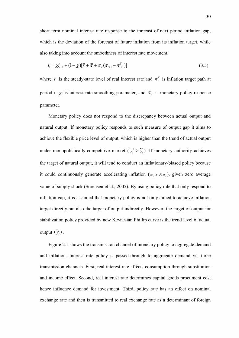
Figure 2.1 shows the transmission channel of monetary policy to aggregate demand
and inflation. Interest rate policy is passed-through to aggregate demand via three
transmission channels. First, real interest rate affects consumption through substitution
and income effect. Second, real interest rate determines capital goods procument cost
hence influence demand for investment. Third, policy rate has an effect on nominal
exchange rate and then is transmitted to real exchange rate as a determinant of foreign
31
demand for domestic good. The latter is also called as monetary transmission through
indirect pass-through effect of exchange rate.
Figure 2.1 Monetary Policy Transmission
Monetary policy is transmitted to consumer inflation through three channels. First,
aggregate demand channel of interest rate policy is passed-through to domestic inflation
through wages. The second channel is interest rate cost of production channel, which is
specifically the interest rate cost of procuring capital goods, either financed by equity or
loan capital. Third, monetary policy affects consumer inflation through two exchange
rate channels. The first one is through the cost of imported intermediate goods in
domestic prices and the other one is through consumption imported-goods inflation.
They are named intermediate and immediate direct pass-through effect of exchange rate
to consumer price, accordingly.
2.2.4 The foreign economy
Foreign demand for domestic goods (exports) is given by the following import demand
function for the foreign economy.
*
*
***
t
t
m
tMtt y
P
Pimx
(4.1)
Consumer
Inflation
Nominal
Interest Rate
Real Capital
Rental Rate
Investment
Consumption
Nominal
Exchange
Rate
Real
Exchange
Rate
Exports
Foreign
Nominal
Interest Rate
Foreign
Price
Imports
Inflation
Real
Import Price
Domestic
Inflation
Real
Wage
Wage
Inflation
Employment
Demand
=
Output
Intermediate
Imports
Goods
Utilized
Capital
Goods
Inflation
Target
Foreign
Demand
Real
Interest Rate
Capital
Depreciation
Rate
32
where *m
tP is the foreign country‘s import price, which is equal to the foreign price of
domestic country‘s exports,
t
x
tm
ts
PP * , where
x
tP is domestic price of domestic
exports and ts is nominal exchange rate in terms of domestic currency per unit of
foreign currency. *
tP is foreign general price level, *
ty is foreign output, *
M is the
share of domestic country‘s export in the rest of the world‘s total demand, and is
price elasticity of exports. By assuming that domestic price of domestic exports, x
tP ,
equals general price level, tP , and substituting for real exchange rate equation
t
ttt
P
Psq
*
, we have
**
ttMt yqx
(4.2)
Foreign output, *
ty , evolves according to stochastic process of the form
tytyyt yyy *,
*
1*
*
*
* lnln)1(ln (4.3)
Where 1> *y >0 and ty*, is serially uncorrelated shock, which is normally distributed
with zero mean and standard deviation *y
Foreign nominal interest rate, *
ti , evolves according to the following stochastic process:
tRtRRt iii *,
*
1*
*
*
* lnln)1(ln (4.4)
Where 1> *R >0 and tR*, is serially uncorrelated shock, which is normally distributed
with zero mean and standard deviation *R
Foreign inflation, *
t , evolves according to the following stochastic process:
ttt *,
*
1*
*
*
* lnln)1(ln (4.5)
33
Where 1> * >0 and t*, is serially uncorrelated shock, which is normally distributed
with zero mean and standard deviation * .
2.2.5 Markets equilibrium
The equilibrium of output goods market is defined by resource constraint that equate
aggregate demand for output with aggregate supply of output (2.2) of the form
MKL rm
ttt
d
ttttttt imkulAimxivgc
)()()( 1 (5.1)
I assume a constant technology and constant stock of goods inventory (zero changes in
inventory). The adjustment of capital utilization makes sure that goods market is always
cleared in the face of shocks. Unlike goods market, labour market is not necessarily
cleared after the occurrence of shocks hence causing the possibility of higher or lower
level of unemployment. Other input goods and money and bond markets are assumed
always cleared.
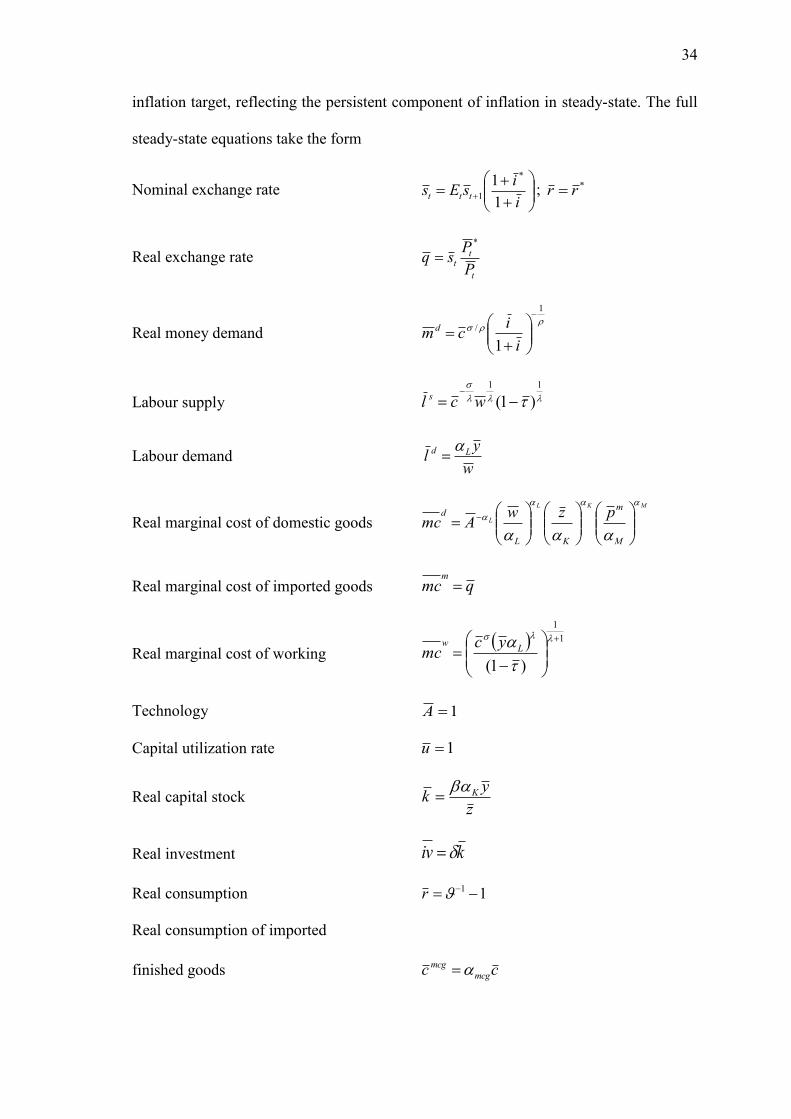
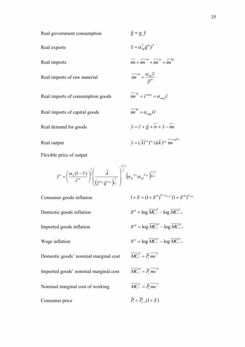
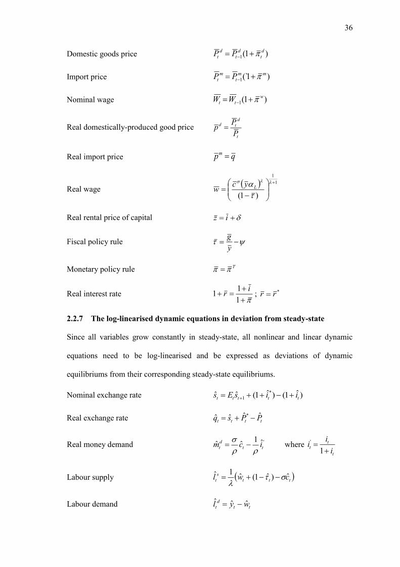
2.2.6 The steady-state equations
In steady-state real variables have zero growth, nominal variables grow at constant rates
and growth variables are stable. Assuming no technological progress or labor force
growth in steady-state, the diminishing returns of capital implies that new capital
produced in steady-state must only need to compensate the existing capital lost due to
depreciation. Therefore, real capital stock stops growing as well, causing the economy
to produce constant real output.
As nominal rigidity vanishes in steady-state, price level is perfectly flexible and is
set at its nominal marginal cost hence real marginal cost stays constant at unity. Thus,
inflation equals changes in nominal marginal cost. The steady-state form of monetary
policy rule equation describes the equality between consumer inflation and exogenous
34
inflation target, reflecting the persistent component of inflation in steady-state. The full
steady-state equations take the form
Nominal exchange rate
i
isEs ttt
1
1 *
1; *rr
Real exchange rate t
tt
P
Psq
*
Real money demand
1
/
1
i
icm d
Labour supply
11
)1(
wcl s
Labour demand w
yl Ld
Real marginal cost of domestic goods
MKL
L
M
m
KL
d pzwAmc
Real marginal cost of imported goods qmcm
Real marginal cost of working 1
1
)1(
Lw yc
mc
Technology 1A
Capital utilization rate 1u
Real capital stock z
yk K
Real investment kiv
Real consumption 11 r
Real consumption of imported
finished goods cc mcg
mcg
35
Real government consumption ygg r
Real exports ** yqx M
Real imports kgcgrm
imimimim
Real imports of raw material m
Mrm
p
yim
Real imports of consumption goods ccim mcg
mcgcg
Real imports of capital goods viim mkg
kg
Real demand for goods imxivgcy
Real output K
KLrm
d imkulAy
)()(
Flexible price of output
L
MK
LMK
MKLn
qz
A
cy
1
1
1
1
)1(
Consumer goods inflation mcgmcg md )1()1(1
)1(
Domestic goods inflation d
t
d
td MCMC 1loglog
Imported goods inflation m
t
m
tm MCMC 1loglog
Wage inflation w
t
w
tw MCMC 1loglog
Domestic goods‘ nominal marginal cost d
t
d
t mcPMC
Imported goods‘ nominal marginal cost m
t
m
t mcPMC
Nominal marginal cost of working w
t
w
t mcPMC
Consumer price )1(1 tt PP
36
Domestic goods price )1(1
d
t
d
t
d
t PP
Import price )1(`1
mm
t
m
t PP
Nominal wage )1(1
w
tt WW
Real domestically-produced good price t
d
td
P
Pp
Real import price qpm
Real wage 1
1
)1(
Lycw
Real rental price of capital iz
Fiscal policy rule y
g
Monetary policy rule T
Real interest rate
1
11
ir ; *rr
2.2.7 The log-linearised dynamic equations in deviation from steady-state
Since all variables grow constantly in steady-state, all nonlinear and linear dynamic
equations need to be log-linearised and be expressed as deviations of dynamic
equilibriums from their corresponding steady-state equilibriums.
Nominal exchange rate )ˆ1()ˆ1(ˆˆ *
1 ttttt iisEs
Real exchange rate tttt PPsq ˆˆˆˆ *
Real money demand 'ˆ1ˆˆ
tt
d
t icm
where
t
tt
i
ii
1
'
Labour supply ttt
s
t cwl ˆ)ˆ1(ˆ1ˆ
Labour demand tt
d
t wyl ˆˆˆ
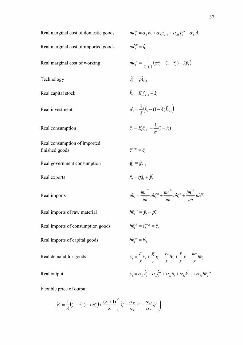
37
Real marginal cost of domestic goods tL
m
tMtKtL
d
t Apzwcm ˆˆˆˆˆ1
Real marginal cost of imported goods t
m
t qcm ˆˆ
Real marginal cost of working ttt
w
t yccm ˆ)ˆ1(ˆ1
1ˆ
Technology 1ˆˆ tt AA
Real capital stock tttt zyEk ˆˆˆ1
Real investment 1ˆ)1(ˆ1
ˆ ttt kkvi
Real consumption )ˆ1(1
ˆˆ1 tttt rcEc
Real consumption of imported
finished goods t
mcg
t cc ˆˆ
Real government consumption 1ˆˆ tt gg
Real exports *ˆˆˆttt yqx
Real imports kg
t
kg
cg
t
cg
rm
t
rm
t miim
immi
im
immi
im
immi ˆˆˆˆ
Real imports of raw material m
tt
rm
t pymi ˆˆˆ
Real imports of consumption goods t
mcg
t
cg
t ccmi ˆˆˆ
Real imports of capital goods t
kg
t vimi ˆˆ
Real demand for goods tttttt mi
y
imx
y
xvi
y
ivg
y
gc
y
cy ˆˆˆˆˆˆ
Real output rm
tMtKtK
d
tLtLt mikulAy ˆˆˆˆˆˆ1
Flexible price of output
n
t
L
Mn
t
L
Kn
t
n
t
n
t
n
t qzAcy ˆˆˆ)1(ˆ)ˆ1(
1ˆ
38
Consumer goods inflation m
tmcgt
d
tmcgt
ate ˆ)ˆ)(1(ˆ
Domestic goods inflation d
t
d
tt
d
t cmE ˆ)1)(1(
ˆˆ1
Imported goods inflation tm
mmm
tt
m
t qE ˆ)1)(1(
ˆˆ1
Wage inflation
ttt
www
w
tt
ww
t
w
www
w
t
yc
E
ˆ)ˆ1(ˆ1
)1)(1)(1(
ˆˆ
)]1(1[
1ˆ
11
Domestic goods‘ nominal marginal cost d
tt
d
t cmPCM ˆˆˆ
Imported goods‘ nominal marginal cost m
tt
m
t cmPCM ˆˆˆ
Nominal marginal cost of working w
tt
w
t cmPCM ˆˆˆ
Consumer price ttt PP ̂ˆˆ1
Domestically-produced goods price d
t
d
t
d
t PP ̂ˆˆ1
Import price m
t
m
t
m
t PP ̂ˆˆ1
Nominal wage w
ttt WW ̂ˆˆ1
Real domestic good price t
d
t
d
t PPp ˆˆˆ
Real import price t
m
t
m
t PPp ˆˆˆ
Flexible real import price )ˆ1(ˆˆ n
t
n
t
mn
t qp
Real wage ttt PWw ˆˆˆ
Flexible real wage ttt
n
t ycw ˆ)ˆ1(ˆ1
1ˆ
Rental rate of capital tt rz
rz ˆˆ
39
Fiscal policy rule
tttt yg
y
gˆˆˆ
1
1ˆ
1
Fiscal policy rule (flexible price)
n
t
n
t
n
t
n
t ygy
gˆˆˆ
1
1ˆ
1
Monetary policy rule T
tttti
ii
)1(ˆˆ1
Monetary policy rule (flexible price) n
t
n
t ii 1ˆˆ
Real interest rate )ˆ1()ˆ1(ˆ1 1 tttt Eir
2.3 Calibration and Solution
2.3.1 Simulation Scenario and Parameter Calibration
I conducted two one-time positive shocks simulations, which are a one percentage
temporary increase in nominal exchange rate and real marginal cost. The former stands
for one percentage depreciation of nominal exchange rate shock from its steady-state
baseline value. The latter represents a certain adverse shock to production cost other
than changes in cost of capital, labour, and importing goods. It is also named as price
mark-up shock as the shock changes the mark-up variable of monopolistically-
competitive domestic producer.
I applied both shocks on two distinct economies, which are different in production
structure, demand structure and degree of domestic and import price rigidities. They are
also different in terms of the sensitivity of labour supply, consumption and money
demand with respect to real wage, real interest rate and nominal interest rate,
respectively, and the level of monetary and fiscal policy target. The feature of the first
economy characterises the structure of advanced economies. The economy has a high
labour input share relative to capital, moderate import content in production and runs a
40
trade deficit. I suppose that nominal wage, import price and domestic price have the
same rigidity, with wages and prices reviewed every year. Monetary authority target is 2
percent of CPI inflation and fiscal authority set the target of fiscal deficit at 1% of GDP.
I henceforth name this economy as ‗advanced‘ economy.
In contrast, the second economy typifies emerging and less developed economies.
Compared to the first economy, the second one has a lower labour share relative to
capital goods in its production structure, but with higher import content in production
and investment. However, it runs a trade surplus as the export-to-GDP ratio is higher
and the share of finished goods imports in total consumption is lower. Consumption
intertemporal elasticity of substitution, wage elasticity of labour supply and interest
elasticity of real money holding are much lower. Import and domestic price are less
rigid than in an ‗advanced‘ economy but have the same degree of rigidity for nominal
wages. However, I assume that import price is less rigid than domestic price, and
domestic price is less rigid than nominal wage. Finally, I assume CPI inflation target
and fiscal deficit ratio are higher than in the previous economy, set at 3% and 2%
respectively. I name this economy as a ‗developing‘ economy, hereafter7.
I subsequently perform monetary policy simulation in order to observe the role of
monetary policy to stabilize the economy following a transient shocks to the nominal
rate of exchange and cost of producing domestic goods. Table 1 describes how the two
economies differ in parameters. All parameter values are fixed by calibration. I follow
other findings on the elasticity of substitution and apply the values for ‗advanced‘
economy. Consumption intertemporal elasticity of substitution is set at 1 =0.5,
interest elasticity of real money holding 1 =0.5, and real wage elasticity of labour
7 The word ‗advanced‘ and ‗developing‘ are in quotes because their economic characteristic are not
intended to be considered as those of the representative advanced and developing economies.
41
supply at 1 =0.67. I calibrate the elasticity paramater for ‗developing‘ economy to
lower than those for ‗advanced‘ economy.
Capital, labour and imported intermediate goods share for ‗advanced‘ economy are
set at 0.28, 0.62, and 0.10. The government spending-to-GDP ratio is 0.18 and export-
to-GDP ratio 0.2. They are closely infered from average ratio of investment-, import-,
export-, and government-to-GDP ratio of UK and US economy. The corresponding
parameter values for ‗developing‘ economy borrow the structure of Indonesia‘s
economy, in which capital‘s, labour‘s and imported intermediate goods‘ share are 0.5,
0.35, and 0.15. The higher share of real capital stock in ‗developing‘ than in ‗advanced‘
economy, )( aK
dK , implies that although the ‗developing‘ economy is less capital
intensive than ‗advanced‘ economy
a
a
d
d
y
k
y
k, real capital stock in ‗developing‘
economy follows ada mkknmk , where d
a
z
zn is ratio of ‗advanced‘ to
‗developing‘ economy‘s real rental rate of capital and a
d
y
ym
is ratio of ‗developing‘
to ‗advanced‘ economy‘s real output.8 The ratios are less than unity because the
‗developing‘ economy‘s interest rate is normally higher than that in ‗advance‘ economy
and the ‗advanced‘ economy‘s output is greater than the ‗developing‘ economy‘s.
Therefore, capital share differential between ‗developing‘ and ‗advanced‘ economy
depends on interest rate and income differential.
A larger capital share than labour share corresponds to a higher cost of capital than
labor cost. We can find that, in the example of Indonesia‘s economy, capital share is
greater than labour share )( WlzPk for capital-to-output ratio equals 3, per capita
8 Capital share: yzkK /
42
annual income (W) equals $1824 and associated values of real GDP and number of
employment. This is consistent with the country‘s gross domestic income that
comprises 64% of gross operating surplus and 34% of compensation of employees. In
contrast, we can find that in a developed economy like the UK, the cost of capital is
lower than labour cost (labour share is greater than capital share), by assuming that the
capital-to-output ratio equals 2.26 (Metz et.al, 2004), nominal wage is approximated by
per capita annual income of twenty three thousand pounds, and lending rate 7.5 APR.
This is in line with the country‘s gross domestic income that comprises 62% of
compensation of employees and 36% of gross operating surplus (Mahajan, 2006).
The firm‘s, importer‘s and wage setter‘s discount factor, , is set at unity. From
consumption Euler equation we get steady-state real interest rate that equals the
household‘s rate of time preference. The setting of real interest rate at 0.02 corresponds
to household discount factor, , at 0.98. Monetary policy response parameter to
inflation gap is set at a value that minimizes the present discounted value of dynamic
welfare loss over fifty quarters after the shock. The loss function is symmetric of the
form
0
22 )()(s
stst
s
Lt yyEL , where monetary policy makers have equal
preferences on both inflation and output stabilization. The inflation feedback parameters
are contingent on the type of shock that hit the economy. The parameter has also to
conform the ―Taylor principles‖ of >1, that the central bank should raise its policy
rate more than one-for-one with increases in inflation.
Figure 2.2 and 2.3 illustrate the welfare loss associated with the range of inflation
response parameter of monetary policy rules that respond to the future inflation gap in
each type of economies. From Figure 2.2 we can calculate that a 0.01 point departure
from the optimal values of inflation response coefficient of monetary policy rules costs
43
additional welfare loss of 0.007 and 0.000005, respectively, in ‗developing‘ and
‗advanced‘ economy. In the case of cost shock in Figure 2.3 the same coefficient
difference from the optimal one increases welfare loss by 0.006 and 0.00015 in
‗developing‘ and ‗advanced‘ economies, correspondingly. It implies that monetary
authority in ‗developing‘ economy faces a higher risk of making non optimal policy
response.
Figure 2.2 Response Parameters and Welfare Loss (Exchange Rate Shock)
‗developing‘ economy ‗advanced‘ economy
The search of optimal inflation feedback parameter is conducted under fixed
interest rate smoothing parameter set at =0.5. This parameter values reflect monetary
authority behaviour that is equally backward- and forward-looking in setting policy rate.
Fiscal policy response parameter is set at =0.5.
Figure 2.3 Response Parameters and Welfare Loss (Cost Shock)
‗developing‘ economy ‗advanced‘ economy
Degree of domestic price rigidity, , is 0.75 for ‗advanced‘ economy and 0.5 for
‗developing‘ economy implying that the average times between domestic price
adjustment are one year and half a year, accordingly. The same rigidity applies for
0
5
10
15
20
25
1 1.2 1.4 1.6 1.8 2 2.2 2.4 2.6 2.8 3
Lo
ss
Response parameter
0
0.002
0.004
0.006
0.008
0.01
0.012
0.014
0.016
0.018
0.02
1 1.1 1.2 1.3 1.4 1.5 1.6 1.7 1.8 1.9 2
Lo
ss
Response parameter
0
5
10
15
20
25
30
35
40
45
50
1 1.1 1.2 1.3 1.4 1.5 1.6 1.7 1.8 1.9 2
Lo
ss
Response parameter
0
0.2
0.4
0.6
0.8
1
1.2
1.4
1 1.1 1.2 1.3 1.4 1.5 1.6 1.7 1.8 1.9 2 2.1 2.2 2.3 2.4 2.5 2.6 2.7 2.8 2.9 3
Lo
ss
Response parameter
44
import price setting in ‗advanced‘ economy (m =0.75), but import price is much less
rigid in ‗developing‘ economy (m =0.3), implying that the average duration of import
price is four months9. The parameter setting is mostly based on and adjusted from two
surveys. Blinder (1991) found that, on average, US prices stay unchanged in one year.
Similar survey for Indonesia‘s economy by Darsono et al. (2002) found that
manufacturing goods prices stay on average of 4.6 months and that exchange rate
changes is passed-through to import price in the same quarter. Finally, wage rigidity is
presumably the same in both economies (w =0.75), corresponding to yearly nominal
wage changes. However, wage changes in ‗developing‘ economy is assumed to heavily
based on previous wage inflation and wage setting behavior in ‗advanced‘ economy is
more forward looking. These assumptions lead me to set parameter w equals 0.9 and
0.25 correspondingly.
Table 2.1
Model Calibration
Parameter
Description
Values
‗advanced‘ ‗developing‘
household‘s discount factor 0.98 0.98
firm‘s, importer‘s and wage setters‘ discount factor
1
1 1 consumption intertemporal elasticity of substitution
0.5
0.008
1 interest elasticity of real money holding 0.6 0.04
1 real wage elasticity of labour supply 0.67 0.02
depreciation rate of capital 0.01 0.01
K dapital share 0.28 0.5
L labour share 0.62 0.35
M imported intermediate input share 0.10 0.15
*
M share of domestic country‘s export in the rest of the
world‘s total demand
0.01
0.01
mcg share of imported consumption good 0.18 0.14
mkg share of imported capital goods investment 0.1 0.14
9 Devereux and Yetman (2005) noted that pass-through in a small open economy is determined by
structural features of the economy, such as the persistence of shocks, and the degree of price stickiness.
45
g ratio of government expenditure-to-output 0.18 0.08
x ratio of exports-to-output 0.2 0.3
price elasticity of exports 0.5 0.1
degree of domestic price stickiness 0.75 0.5
m degree of import price stickiness 0.75 0.3
w degree of wage stickiness 0.75 0.75
w degree of wage indexation to lag inflation 0.25 0.9
target of fiscal deficit ratio 1% 2%
T target of consumer inflation 2% 3%
degree of interest rate inertia 0.5 0.5
monetary policy response parameter
- exchange rate shock 1.52 1.63
- cost shock 2.11 1.6
fiscal policy response parameter 0.5 0.5
2.3.2 Model Solution
In this research I solved the static steady-state model and the log-linearised dynamic
model in deviation from steady-state using CONOPT solver under GAMS system. This
solver employs Generalized Reduced Gradient method of solution for nonlinear
programming problems defined as:
min or max f(z)=J=0 (performance index) (6.1)
subject to vector of implicit log-linear functions
)(zg = )( x,yθ,;x,y,y,y t1tt1t tg =
)(
)(
,
,1
x,yθ,;x,y,y,y
x,yθ,;x,y,y,y
t1tt1t
t1tt1t
tm
t
g
g
= 0 (6.2)
uzl (6.3)
where z is vector of optimization variables, l and u are vectors of lower and upper
bounds, some of which may be minus or plus infinity, and f and g are differentiable
nonlinear functions that define the model. Constraint (6.2) is general constraints and
(6.3) is boundary of variables. The objective function f is the variable to be minimized
or maximized; m is the number of equations and n denotes number of variables. Vector
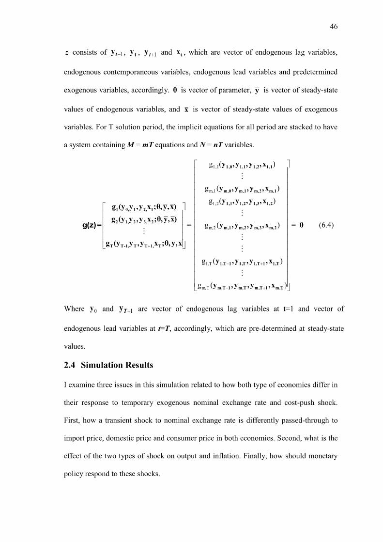
46
z consists of 1ty , ty , 1ty and tx , which are vector of endogenous lag variables,
endogenous contemporaneous variables, endogenous lead variables and predetermined
exogenous variables, accordingly. θ is vector of parameter, y is vector of steady-state
values of endogenous variables, and x is vector of steady-state values of exogenous
variables. For T solution period, the implicit equations for all period are stacked to have
a system containing M = mT equations and N = nT variables.
g(z)=
x,yθ,;xy,y(yg
)x,yθ,;xy,y(yg
)x,yθ,;xy,y(yg
T1,TT1,-TT
23,21,2
12,10,1
=
)(g
)(g
)(g
)(g
)(g
)(g
Tm,
T1,
m,2
1,2
m,1
1,1
Tm,1Tm,Tm,1Tm,
T1,1T1,T1,1T1,
m,2m,3m,2m,1
1,21,31,21,1
m,1m,2m,1m,0
1,11,21,11,0
x,y,y,y
x,y,y,y
x,y,y,y
x,y,y,y
x,y,y,y
x,y,y,y
= 0 (6.4)
Where 0y and 1Ty are vector of endogenous lag variables at t=1 and vector of
endogenous lead variables at t=T, accordingly, which are pre-determined at steady-state
values.
2.4 Simulation Results
I examine three issues in this simulation related to how both type of economies differ in
their response to temporary exogenous nominal exchange rate and cost-push shock.
First, how a transient shock to nominal exchange rate is differently passed-through to
import price, domestic price and consumer price in both economies. Second, what is the
effect of the two types of shock on output and inflation. Finally, how should monetary
policy respond to these shocks.
47
I apply shock simulation to the log-linearised version of the model in deviation
from steady-state values. As the lag dependent variables take their steady-state values, it
means the shocks simulatedly occur in the steady-state of the economy, in which the
level of real variables and growth variables, i.e. inflation, are constant, and the level of
nominal variables grows at nonzero constant rates. Hence we need to interpret the
simulation result for the actual shocks that occur in the economy before the steady-state,
in which the level of real and nominal variables can grow at nonzero rates and the level
of growth variables are not necessarily constant.
Figure 2.4 Illustration of shock simulation to a real variable
When we apply a one-time shock in steady-state, the resulted deviation of a real
variable from its constant steady-state equilibrium value means either an expansion or a
contraction of the level of such real variable. However, when the shock occurs in
dynamic state of the economy, which is before steady-state, it will generally result in
either an accelerated or a decelerated level of a real variable except that the magnitude
History Projection
xt
xss
t
Steady-state
A one-time shock in
steady-state contract
the level of xt
A one-time shock before
steady-state decreases
the growth of xt (can be
contracting)
Deviation of dynamic equilibrium of the level of
real variable x from its
steady-state equilibrium
(xt - xss)
48
of shock is large enough to contract real variables. Therefore, one may interpret an
expansion or a contraction of a real variable in steady-state as an increasing or a
decreasing growth of a real variable before steady-state. Figure 2.4 illustrates the
interpretation of the contraction effect on a given real variable of a one-time simulated
shock in steady-state. We can infer similar interpretation for a nominal variable in the
case of a one-time shock, in steady-state (Figure 2.5). Meanwhile, the interpretation of
the effect on a growth variable of a one-time shock in steady-state is the same with of a
one-time actual shock before the steady-state.
Figure 2.5 Illustration of shock simulation to a nominal variable
2.4.1 One-Time Nominal Exchange Rate Shock
We can define exchange rate pass-through in several ways as in the literature. The first
one is the narrow definition as, for example, in Campa and Goldberg (2001) that define
exchange rate pass-through as how changes in exchange rate are transmitted to imported
goods prices. The broader definition of exchange rate pass-through as, for example, in
History Projection
Xt
Xtss
t
Steady-state
A one-time shock in
steady-state decreases
the growth of Xt (in
this case, a negative
growth)
A one-time shock before
steady-state decreases the
growth of Xt
Deviation of dynamic equilibrium of the level of nominal variable X
from its steady-state equilibrium
(Xt - Xtss)
49
Devereux (2001) and Devereux and Yetman (2003) is the transmission of exchange rate
changes to domestic inflation. It reflects indirect pass-through of exchange rate to CPI
price level through changes in aggregate demand and cost of production. Finally, the
most general definition reflects the farthest and complete transmission of exchange rate
to CPI inflation through the price of imported intermediate goods, domestically
produced goods, and imported consumption goods. It covers both direct and indirect
pass-through through domestic inflation and direct pass-through through imported
consumption goods inflation.
Figure 2.8 shows the simulation result under the assumption of fully forward
looking price setter. The short-run exchange rate pass-through to import price in
‗developing‘ economy is much higher than that in ‗advanced‘ economy. It is due to the
effect of lower import price rigidity in ‗developing‘ economy. One percent of nominal
exchange rate depreciation from steady-state level increases import price by 1.41
percent in the quarter when the shock occurs. However, import price decreases below its
steady-state level in the quarters following the shock as real exchange rate appreciates
from its steady-state value. In ‗advanced‘ economy, the immediate short-run exchange
rate pass-through to import price is 0.077 meaning that only 7.7% of one-time nominal
exchange rate shock is passed-through to import price at the immediate quarter.
Domestic price in ‗developing‘ economy increases to a peak level of 0.22 percent
deviation from steady-state at 9th
quarters. It finally stays slightly below initial steady-
state in the long run. The price of domestically produced goods in ‗advanced‘ economy
gradually increases to a peak level of 0.0053 percent deviation from its steady-state at
18th
quarters, then decreases to a slightly new higher steady-state in the long run. The
existence of nominal wage stickiness amplifies the role of domestic price rigidity in
absorbing the impact of nominal exchange rate shock to domestic price. In domestic
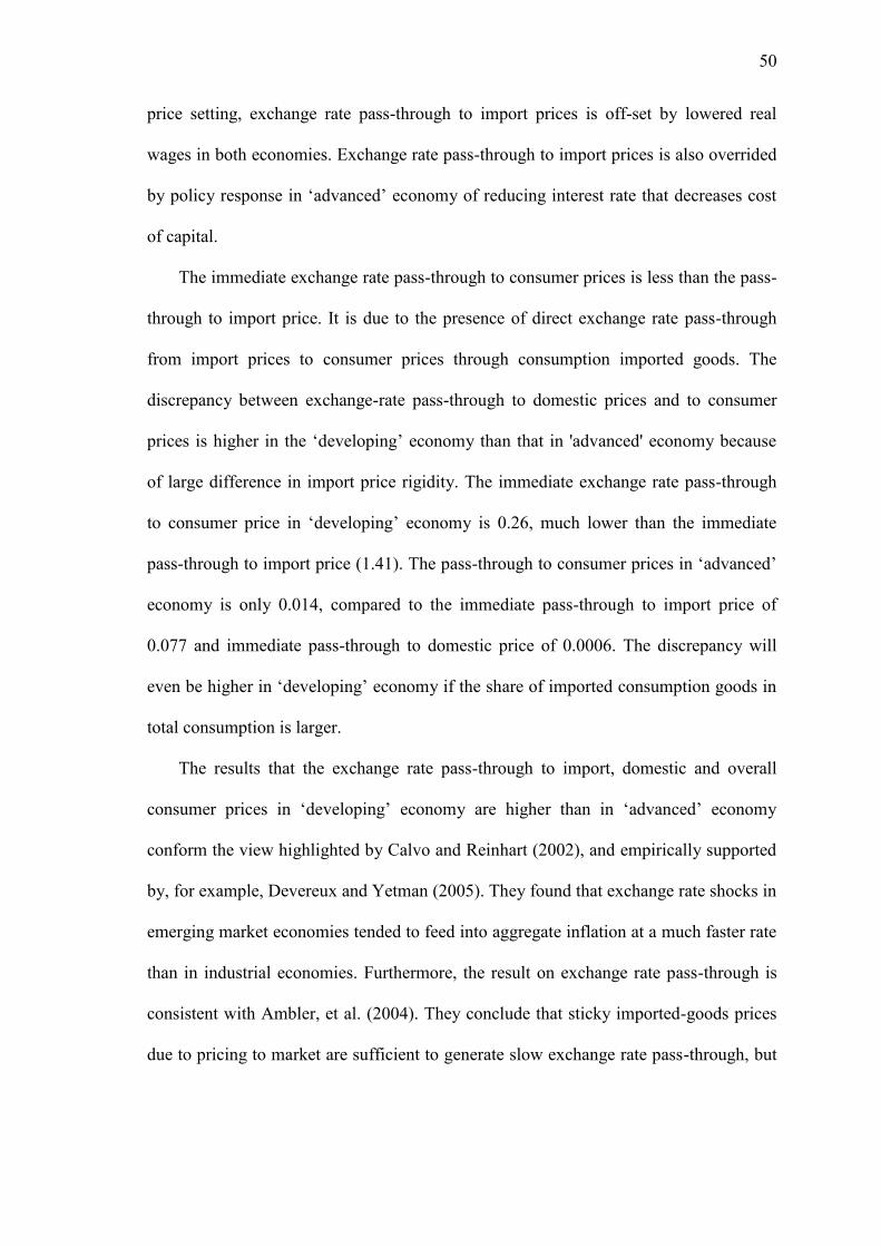
50
price setting, exchange rate pass-through to import prices is off-set by lowered real
wages in both economies. Exchange rate pass-through to import prices is also overrided
by policy response in ‗advanced‘ economy of reducing interest rate that decreases cost
of capital.
The immediate exchange rate pass-through to consumer prices is less than the pass-
through to import price. It is due to the presence of direct exchange rate pass-through
from import prices to consumer prices through consumption imported goods. The
discrepancy between exchange-rate pass-through to domestic prices and to consumer
prices is higher in the ‗developing‘ economy than that in 'advanced' economy because
of large difference in import price rigidity. The immediate exchange rate pass-through
to consumer price in ‗developing‘ economy is 0.26, much lower than the immediate
pass-through to import price (1.41). The pass-through to consumer prices in ‗advanced‘
economy is only 0.014, compared to the immediate pass-through to import price of
0.077 and immediate pass-through to domestic price of 0.0006. The discrepancy will
even be higher in ‗developing‘ economy if the share of imported consumption goods in
total consumption is larger.
The results that the exchange rate pass-through to import, domestic and overall
consumer prices in ‗developing‘ economy are higher than in ‗advanced‘ economy
conform the view highlighted by Calvo and Reinhart (2002), and empirically supported
by, for example, Devereux and Yetman (2005). They found that exchange rate shocks in
emerging market economies tended to feed into aggregate inflation at a much faster rate
than in industrial economies. Furthermore, the result on exchange rate pass-through is
consistent with Ambler, et al. (2004). They conclude that sticky imported-goods prices
due to pricing to market are sufficient to generate slow exchange rate pass-through, but
51
not necessary as nominal wage and domestic prices rigidities also result in slow
exchange rate pass-through to consumer price.
The central bank in ‗advanced‘ economy needs to respond to the after-shocks
lowered expected inflation by decreasing interest rate contemporaneously and returning
it back to around the steady-state level in the long run. However, the ex-ante real
interest rate increases due to expected future lower inflation that is less than decreases
in nominal interest rates. The upward adjustment in real interest rate lowers
consumption and investment. Nominal exchange rate shock boosts exports but reduces
imports causing an increase in net exports that outweighs decreases in consumption and
investment. Therefore, one-time exchange rate depreciation can have expansionary
effect on output in ‗advanced‘ economy.
Nominal interest rate in ‗developing‘ economy is slightly increased and stays above
the steady-state in the early periods after shock. On the other hand, consumer inflation
is still above the steady-state several periods after the shocks resulting in an immediate
slightly lower real interest rate. However, the smaller real interest rate has an
insignificant effect on consumption as consumption intertemporal elasticity of
substitution is exceedingly small. Thus, consumption slightly decreases. Investment also
contracts since the expected lower future demand for output is larger than the decreases
in real rental rate of capital. Unfortunately, exchange rate depreciation does not boost up
exports much while imports suffer. The immediate net effect of depreciation on
‗developing‘ economy‘s output is expansionary followed by contractionary.
By varying monetary policy response parameters, we can find short run trade-off
between inflation gap and output gap (Figure 2.6). A more active monetary policy, in
this case the one that result in a larger nominal interest rate decline, leads to a higher
short run output expansion but at the cost of higher increase in inflation. This finding is
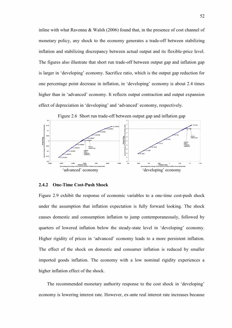
52
inline with what Ravenna & Walsh (2006) found that, in the presence of cost channel of
monetary policy, any shock to the economy generates a trade-off between stabilizing
inflation and stabilizing discrepancy between actual output and its flexible-price level.
The figures also illustrate that short run trade-off between output gap and inflation gap
is larger in ‗developing‘ economy. Sacrifice ratio, which is the output gap reduction for
one percentage point decrease in inflation, in ‗developing‘ economy is about 2.4 times
higher than in ‗advanced‘ economy. It reflects output contraction and output expansion
effect of depreciation in ‗developing‘ and ‗advanced‘ economy, respectively.
Figure 2.6 Short run trade-off between output gap and inflation gap
‗advanced‘ economy ‗developing‘ economy
2.4.2 One-Time Cost-Push Shock
Figure 2.9 exhibit the response of economic variables to a one-time cost-push shock
under the assumption that inflation expectation is fully forward looking. The shock
causes domestic and consumption inflation to jump contemporaneously, followed by
quarters of lowered inflation below the steady-state level in ‗developing‘ economy.
Higher rigidity of prices in ‗advanced‘ economy leads to a more persistent inflation.
The effect of the shock on domestic and consumer inflation is reduced by smaller
imported goods inflation. The economy with a low nominal rigidity experiences a
higher inflation effect of the shock.
The recommended monetary authority response to the cost shock in ‗developing‘
economy is lowering interest rate. However, ex-ante real interest rate increases because
1.0; 0.013035
1.1; 0.008574
1.2; 0.005049
1.3; 0.002473
1.4; 0.000857
1.52; 0.000198
1.6; 0.000537
1.7; 0.001826
1.8; 0.00402
1.9; 0.006922
2.0; 0.00976
-0.2
-0.15
-0.1
-0.05
0
0.05
0.1
0.15
0.2
0.056 0.057 0.058 0.059 0.06 0.061 0.062
Ou
tpu
t G
ap
(perc
en
t ch
an
ge o
f fi
rst
peri
od
GD
P fro
m its
ste
ad
y-s
tate
)
Inflation Gap (percentage point change of first period consumer inflation from steady-state)
optimalpolicyresponse coefficient
PDV of welfare loss
1.0; 19.83
1.1; 14.99
1.2; 10.58
1.3; 6.71
1.4; 3.54
1.5; 1.25
1.63; 0.06
1.8; 0.44
-8
-7
-6
-5
-4
-3
-2
-1
0
1
2
0.8 0.85 0.9 0.95 1 1.05 1.1 1.15
Ou
tpu
t G
ap
(perc
en
t ch
an
ge o
f fi
rst
peri
od
GD
P fro
m s
tead
y-s
tate
)
Inflation Gap (percentage point change of first period consumer inflation from steady-state)
optimalpolicyresponse coefficient
PDV of welfare loss
53
expected future inflation is much lower than decreases in nominal interest rate. Inflation
in ‗developing‘ economy is easier to get lower than in ‗advanced‘ economy since
domestic price in this economy is assumed to be symmetrically less rigid than in
‗advanced‘ economy. As a result, investment and consumption go down
contemporaneously. As the shock lowers the relative price between foreign and
domestic goods in larger magnitude than nominal exchange rate depreciation, real
exchange rate appreciates. Consequently, external demand for domestic goods declines.
Thus, the cost shock effect on output and employment is contractionary.
Figure 2.7 Short run trade-off between output gap and inflation gap
‗advanced‘ economy ‗developing‘ economy
Following the price increases caused by a shock to marginal cost, monetary
authority in ‗advanced‘ economy should slightly increase nominal interest rate.
However, inflation is more persistent in the subsequent period that results in an
immediate lower real interest rate. However, consumption goes down because the effect
of expected future consumption is greater than of real interest rate. Expected output also
dominates real rental rate of capital in affecting demand for capital goods and
investment. Combined with the effect of real exchange rate appreciation on exports, the
cost shock effect on ‗advanced‘ economy‘s output is also contractionary.
This shock simulation also found a short-run trade-off between inflation gap and
output gap in both economies (Figure 2.7). A higher monetary policy response
coefficient, which corresponds to a larger decline in nominal interest rate, leads to a
1.0; 1.198
1.1; 1.002
1.2; 0.823
1.3; 0.661
1.4; 0.517
1.5; 0.390
1.6; 0.281
1.7; 0.190
1.8; 0.118
1.9; 0.064
2.0; 0.030
2.11; 0.015
2.2; 0.027
2.3; 0.067
2.4; 0.117
2.5; 0.1692.6; 0.216
2.8; 0.2963.0; 0.357
-2
-1.5
-1
-0.5
0
0.5
1
0.235 0.24 0.245 0.25 0.255 0.26 0.265 0.27
Ou
tpu
t G
ap
(perc
en
t ch
an
ge o
f G
DP
fro
m f
rom
ste
ad
y-s
tate
)
Inflation Gap(percentage point change of consumer inflation from steady-state)
optimal policy response coefficient
PDV of welfare loss
1.0; 44.6
1.1; 34.9
1.2; 25.9
1.3; 17.8
1.4, 10.8
1.5,5.2
1.5, 1.48
1.71; 0.18
2.0, 1.4
-10
-8
-6
-4
-2
0
2
4
1.1 1.15 1.2 1.25 1.3 1.35 1.4 1.45 1.5 1.55
Ou
tpu
t G
ap
(perc
en
t ch
an
ge o
f G
DP
fro
m f
rom
ste
ad
y-s
tate
)
Inflation Gap(percentage point change of consumer inflation from steady-state)
optimalpolicy response coefficient
PDVof welfare loss
54
higher output expansion and a higher inflation. Sacrifice ratio in ‗developing‘ economy
is about 3 times higher than in ‗advanced‘ economy.
2.5 Conclusion
In this paper I investigate how economic players in two distinctive open economies
behave differently in responding to one-time exogenous shock to nominal exchange rate
and cost of production, using a new Keynesian dynamic general equilibrium model that
features wage and prices stickiness and includes cost channel of monetary policy to
inflation. The economies differ in the structure of economic output, sensitivity of
agents‘ economic decision on price of money, goods and labour, and most importantly,
in degree of nominal prices and wage rigidity.
Regarding the effect of exchange rate shocks on inflation, I found that degree of
import price rigidity is not the only factor that affects the strength of exchange rate pass-
through to consumer inflation. It is also affected by degree of nominal wage and
domestic price stickiness, degree of production dependency on imported input, share of
imported consumption goods in total consumption, and monetary policy response. A
lower wage and prices stickiness, higher dependency on imports and a more loose
monetary policy, will worsen the effect of temporary nominal exchange rate
depreciation to consumer prices.
The finding with regard to monetary policy response to cost shock is different with
the result in Clarida et al. (1999). They show that in the presence of exogenous cost-
push shock, the near-term inflation can only be reduced by increasing interest rate.
Consequently, they conclude that an extreme inflation targeting, in the sense that the
policy is adjusted to reach an inflation target immediately, is optimal under only one of
two circumstances: (1) cost push inflation is absent; or (2) there is no concern for output
deviations. In contrast, this paper shows that the transitory nature of cost-push shock
55
combined with rational expectation behaviour of price setter, symmetric low rigidity of
domestic price and less persistence of inflation does not lead the monetary authority in
‗developing‘ economy to immediately respond to the shock by conducting tight
monetary policy.
Finally, it is essential to point out that, the findings in this paper, particularly on the
monetary policy implication, might be dissimilar under the presence of covered interest
rate parity and when the shock is more persistent. Moreover, it could be intriguing to
investigate the policy implication under lower input price elasticity of demand for factor
input.
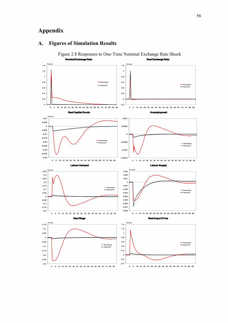
56
Appendix
A. Figures of Simulation Results
Figure 2.8 Responses to One-Time Nominal Exchange Rate Shock
0
0.2
0.4
0.6
0.8
1
1.2
1.4
0 5 10 15 20 25 30 35 40 45 50 55 60 65 70 75 80 85 90
Nominal Exchange Rate
'Developing'
'Advanced'
Percent
-0.2
0
0.2
0.4
0.6
0.8
1
1.2
0 5 10 15 20 25 30 35 40 45 50 55 60 65 70 75 80 85
Real Exchange Rate
'Developing'
'Advanced'
Percent
-0.04
-0.035
-0.03
-0.025
-0.02
-0.015
-0.01
-0.005
0
0.005
0.01
0 5 10 15 20 25 30 35 40 45 50 55 60 65 70 75 80 85
Real Capital Goods
'Developing'
'Advanced'
Percent
-0.0015
-0.001
-0.0005
0
0.0005
0.001
0 5 10 15 20 25 30 35 40 45 50 55 60 65 70 75 80 85
Unemployment
'Developing'
'Advanced'
-0.2
-0.15
-0.1
-0.05
0
0.05
0.1
0.15
0.2
0.25
0.3
0.35
0 5 10 15 20 25 30 35 40 45 50 55 60 65 70 75 80 85
Labour Demand
'Developing'
'Advanced'
Percent
-0.008
-0.007
-0.006
-0.005
-0.004
-0.003
-0.002
-0.001
0
0.001
0.002
0.003
0 5 10 15 20 25 30 35 40 45 50 55 60 65 70 75 80 85
Labour Supply
'Developing'
'Advanced'
Percent
-0.3
-0.25
-0.2
-0.15
-0.1
-0.05
0
0.05
0.1
0.15
0 5 10 15 20 25 30 35 40 45 50 55 60 65 70 75 80 85
Real Wage
'Developing'
'Advanced'
Percent
-0.4
-0.2
0
0.2
0.4
0.6
0.8
1
1.2
1.4
0 5 10 15 20 25 30 35 40 45 50 55 60 65 70 75 80 85
Real Import Price
'Developing'
'Advanced'
Percent
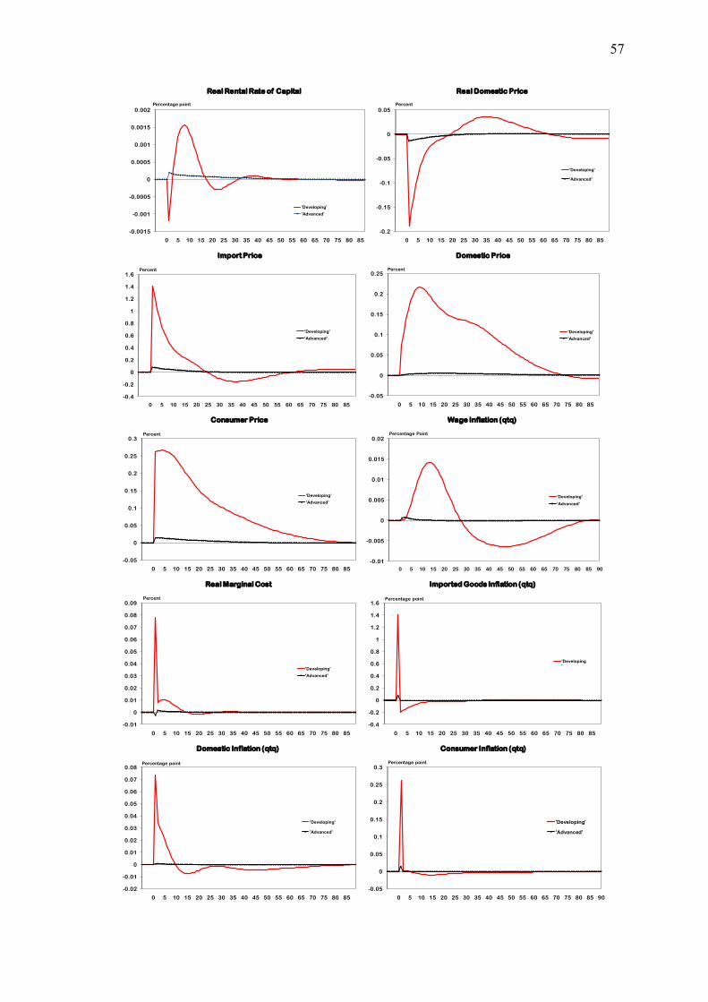
57
-0.0015
-0.001
-0.0005
0
0.0005
0.001
0.0015
0.002
0 5 10 15 20 25 30 35 40 45 50 55 60 65 70 75 80 85
Percentage point
Real Rental Rate of Capital
'Developing'
'Advanced'
-0.2
-0.15
-0.1
-0.05
0
0.05
0 5 10 15 20 25 30 35 40 45 50 55 60 65 70 75 80 85
Real Domestic Price
'Developing'
'Advanced'
Percent
-0.4
-0.2
0
0.2
0.4
0.6
0.8
1
1.2
1.4
1.6
0 5 10 15 20 25 30 35 40 45 50 55 60 65 70 75 80 85
Import Price
'Developing'
'Advanced'
Percent
-0.05
0
0.05
0.1
0.15
0.2
0.25
0 5 10 15 20 25 30 35 40 45 50 55 60 65 70 75 80 85
Domestic Price
'Developing'
'Advanced'
Percent
-0.05
0
0.05
0.1
0.15
0.2
0.25
0.3
0 5 10 15 20 25 30 35 40 45 50 55 60 65 70 75 80 85
Consumer Price
'Developing'
'Advanced'
Percent
-0.01
-0.005
0
0.005
0.01
0.015
0.02
0 5 10 15 20 25 30 35 40 45 50 55 60 65 70 75 80 85 90
Wage Inflation (qtq)
'Developing'
'Advanced'
Percentage Point
-0.01
0
0.01
0.02
0.03
0.04
0.05
0.06
0.07
0.08
0.09
0 5 10 15 20 25 30 35 40 45 50 55 60 65 70 75 80 85
Real Marginal Cost
'Developing'
'Advanced'
Percent
-0.4
-0.2
0
0.2
0.4
0.6
0.8
1
1.2
1.4
1.6
0 5 10 15 20 25 30 35 40 45 50 55 60 65 70 75 80 85
Imported Goods Inflation (qtq)
'Developing'
Percentage point
-0.02
-0.01
0
0.01
0.02
0.03
0.04
0.05
0.06
0.07
0.08
0 5 10 15 20 25 30 35 40 45 50 55 60 65 70 75 80 85
Domestic Inflation (qtq)
'Developing'
'Advanced'
Percentage point
-0.05
0
0.05
0.1
0.15
0.2
0.25
0.3
0 5 10 15 20 25 30 35 40 45 50 55 60 65 70 75 80 85 90
Consumer Inflation (qtq)
'Developing'
'Advanced'
Percentage point
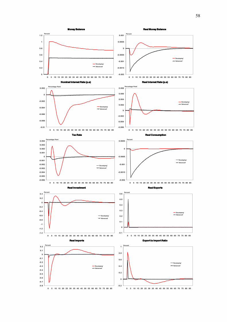
58
0
0.2
0.4
0.6
0.8
1
1.2
0 5 10 15 20 25 30 35 40 45 50 55 60 65 70 75 80 85
Money Balance
'Developing'
'Advanced'
Percent
-0.002
-0.0015
-0.001
-0.0005
0
0.0005
0.001
0 5 10 15 20 25 30 35 40 45 50 55 60 65 70 75 80 85
Real Money Balance
'Developing'
'Advanced'
Percent
-0.01
-0.008
-0.006
-0.004
-0.002
0
0.002
0 5 10 15 20 25 30 35 40 45 50 55 60 65 70 75 80 85
Nominal Interest Rate (p.a)
'Developing'
'Advanced'
Percentage Point
-0.006
-0.004
-0.002
0
0.002
0.004
0.006
0.008
0 5 10 15 20 25 30 35 40 45 50 55 60 65 70 75 80 85
Real Interest Rate (p.a)
'Developing'
'Advanced'
Percentage Point
-0.006
-0.005
-0.004
-0.003
-0.002
-0.001
0
0.001
0.002
0.003
0.004
0 5 10 15 20 25 30 35 40 45 50 55 60 65 70 75 80 85
Tax Rate
'Developing'
'Advanced'
Percentage Point
-0.002
-0.0015
-0.001
-0.0005
0
0.0005
0 5 10 15 20 25 30 35 40 45 50 55 60 65 70 75 80 85
Real Consumption
'Developing'
'Advanced'
Percent
-1.4
-1.2
-1
-0.8
-0.6
-0.4
-0.2
0
0.2
0.4
0 5 10 15 20 25 30 35 40 45 50 55 60 65 70 75 80 85
Percent
Real Investment
'Developing'
'Advanced'
-0.1
0
0.1
0.2
0.3
0.4
0.5
0.6
0 5 10 15 20 25 30 35 40 45 50 55 60 65 70 75 80 85
Real Exports
'Developing'
'Advanced'
Percent
-0.8
-0.7
-0.6
-0.5
-0.4
-0.3
-0.2
-0.1
0
0.1
0.2
0 5 10 15 20 25 30 35 40 45 50 55 60 65 70 75 80 85
Real Imports
'Developing'
'Advanced'
Percent
-0.2
0
0.2
0.4
0.6
0.8
1
0 5 10 15 20 25 30 35 40 45 50 55 60 65 70 75 80 85
Export to Import Ratio
'Developing'
'Advanced'
Percent
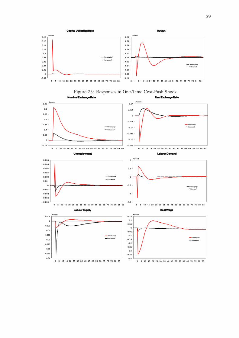
59
Figure 2.9 Responses to One-Time Cost-Push Shock
-0.02
0
0.02
0.04
0.06
0.08
0.1
0.12
0.14
0.16
0.18
0 5 10 15 20 25 30 35 40 45 50 55 60 65 70 75 80 85
Capital Utilisation Rate
'Developing'
'Advanced'
Percent
-0.10
-0.08
-0.06
-0.04
-0.02
0.00
0.02
0.04
0.06
0.08
0.10
0 1 6 11 16 21 26 31 36 41 46 51 56 61 66 71 76 81 86
Output
'Developing'
'Advanced'
Percent
-0.05
0
0.05
0.1
0.15
0.2
0.25
0.3
0.35
0 5 10 15 20 25 30 35 40 45 50 55 60 65 70 75 80 85 90
Nominal Exchange Rate
'Developing'
'Advanced'
Percent
-0.025
-0.02
-0.015
-0.01
-0.005
0
0.005
0.01
0 5 10 15 20 25 30 35 40 45 50 55 60 65 70 75 80 85
Real Exchange Rate
'Developing'
'Advanced'
Percent
-0.004
-0.003
-0.002
-0.001
0
0.001
0.002
0.003
0.004
0.005
0.006
0 5 10 15 20 25 30 35 40 45 50 55 60 65 70 75 80 85 90
Unemployment
'Developing'
'Advanced'
-1.5
-1
-0.5
0
0.5
1
0 5 10 15 20 25 30 35 40 45 50 55 60 65 70 75 80 85
Labour Demand
'Developing'
'Advanced'
Percent
-0.04
-0.035
-0.03
-0.025
-0.02
-0.015
-0.01
-0.005
0
0.005
0 5 10 15 20 25 30 35 40 45 50 55 60 65 70 75 80 85
Labour Supply
'Developing'
'Advanced'
Percent
-0.4
-0.35
-0.3
-0.25
-0.2
-0.15
-0.1
-0.05
0
0.05
0.1
0.15
0 5 10 15 20 25 30 35 40 45 50 55 60 65 70 75 80 85
Real Wage
'Developing'
'Advanced'
Percent
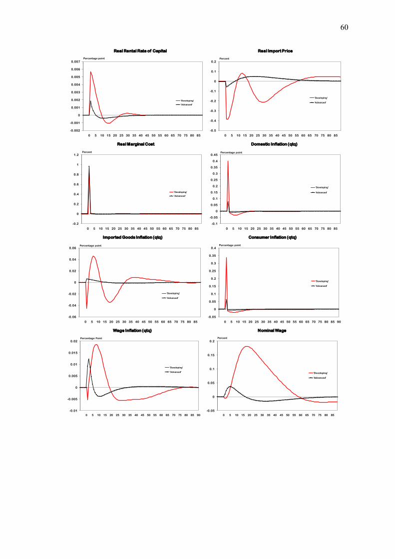
60
-0.002
-0.001
0
0.001
0.002
0.003
0.004
0.005
0.006
0.007
0 5 10 15 20 25 30 35 40 45 50 55 60 65 70 75 80 85
Percentage point
Real Rental Rate of Capital
'Developing'
'Advanced'
-0.5
-0.4
-0.3
-0.2
-0.1
0
0.1
0.2
0 5 10 15 20 25 30 35 40 45 50 55 60 65 70 75 80 85
Real Import Price
'Developing'
'Advanced'
Percent
-0.2
0
0.2
0.4
0.6
0.8
1
1.2
0 5 10 15 20 25 30 35 40 45 50 55 60 65 70 75 80 85
Real Marginal Cost
'Developing'
'Advanced'
Percent
-0.1
-0.05
0
0.05
0.1
0.15
0.2
0.25
0.3
0.35
0.4
0.45
0 5 10 15 20 25 30 35 40 45 50 55 60 65 70 75 80 85
Domestic Inflation (qtq)
'Developing'
'Advanced'
Percentage point
-0.06
-0.04
-0.02
0
0.02
0.04
0.06
0 5 10 15 20 25 30 35 40 45 50 55 60 65 70 75 80 85
Imported Goods Inflation (qtq)
'Developing'
'Advanced'
Percentage point
-0.05
0
0.05
0.1
0.15
0.2
0.25
0.3
0.35
0.4
0 5 10 15 20 25 30 35 40 45 50 55 60 65 70 75 80 85 90
Consumer Inflation (qtq)
'Developing'
'Advanced'
Percentage point
-0.01
-0.005
0
0.005
0.01
0.015
0.02
0 5 10 15 20 25 30 35 40 45 50 55 60 65 70 75 80 85 90
Wage Inflation (qtq)
'Developing'
'Advanced'
Percentage Point
-0.05
0
0.05
0.1
0.15
0.2
0 5 10 15 20 25 30 35 40 45 50 55 60 65 70 75 80 85
Nominal Wage
'Developing'
'Advanced'
Percent
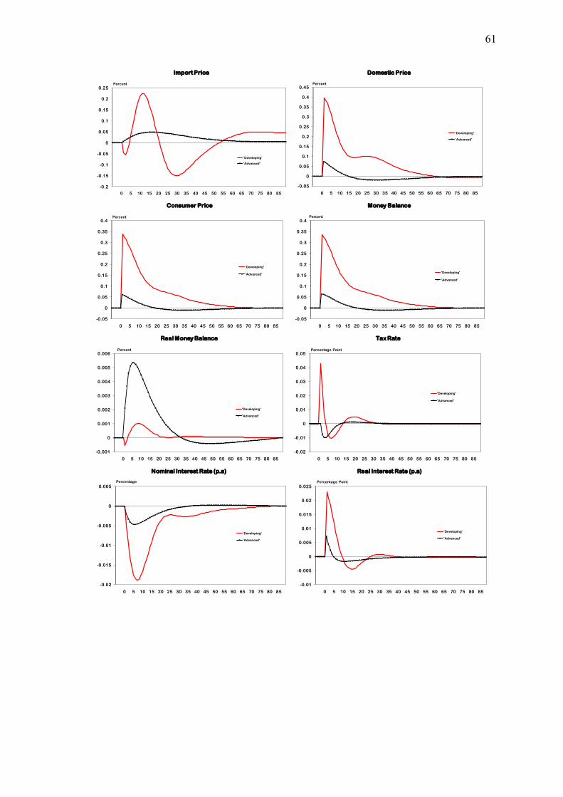
61
-0.2
-0.15
-0.1
-0.05
0
0.05
0.1
0.15
0.2
0.25
0 5 10 15 20 25 30 35 40 45 50 55 60 65 70 75 80 85
Import Price
'Developing'
'Advanced'
Percent
-0.05
0
0.05
0.1
0.15
0.2
0.25
0.3
0.35
0.4
0.45
0 5 10 15 20 25 30 35 40 45 50 55 60 65 70 75 80 85
Domestic Price
'Developing'
'Advanced'
Percent
-0.05
0
0.05
0.1
0.15
0.2
0.25
0.3
0.35
0.4
0 5 10 15 20 25 30 35 40 45 50 55 60 65 70 75 80 85
Consumer Price
'Developing'
'Advanced'
Percent
-0.05
0
0.05
0.1
0.15
0.2
0.25
0.3
0.35
0.4
0 5 10 15 20 25 30 35 40 45 50 55 60 65 70 75 80 85
Money Balance
'Developing'
'Advanced'
Percent
-0.001
0
0.001
0.002
0.003
0.004
0.005
0.006
0 5 10 15 20 25 30 35 40 45 50 55 60 65 70 75 80 85
Real Money Balance
'Developing'
'Advanced'
Percent
-0.02
-0.01
0
0.01
0.02
0.03
0.04
0.05
0 5 10 15 20 25 30 35 40 45 50 55 60 65 70 75 80 85
Tax Rate
'Developing'
'Advanced'
Percentage Point
-0.02
-0.015
-0.01
-0.005
0
0.005
0 5 10 15 20 25 30 35 40 45 50 55 60 65 70 75 80 85
Nominal Interest Rate (p.a)
'Developing'
'Advanced'
Percentage
-0.01
-0.005
0
0.005
0.01
0.015
0.02
0.025
0 5 10 15 20 25 30 35 40 45 50 55 60 65 70 75 80 85
Real Interest Rate (p.a)
'Developing'
'Advanced'
Percentage Point
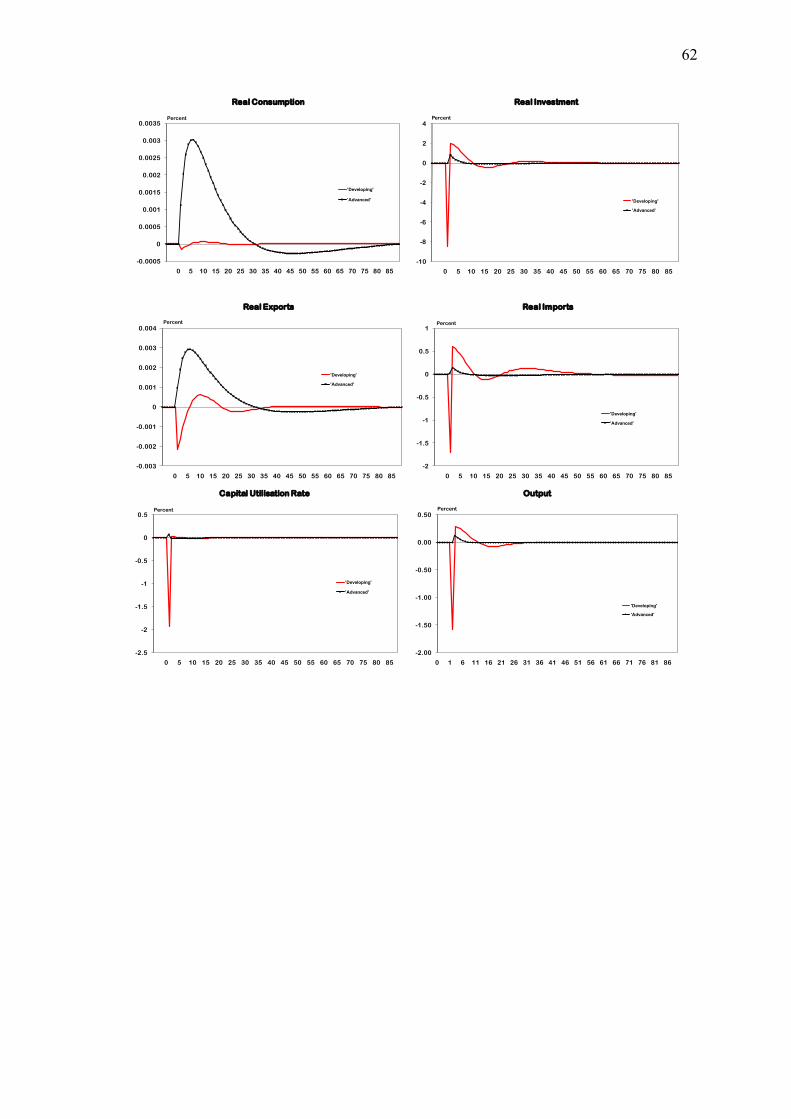
62
-0.0005
0
0.0005
0.001
0.0015
0.002
0.0025
0.003
0.0035
0 5 10 15 20 25 30 35 40 45 50 55 60 65 70 75 80 85
Real Consumption
'Developing'
'Advanced'
Percent
-10
-8
-6
-4
-2
0
2
4
0 5 10 15 20 25 30 35 40 45 50 55 60 65 70 75 80 85
Percent
Real Investment
'Developing'
'Advanced'
-0.003
-0.002
-0.001
0
0.001
0.002
0.003
0.004
0 5 10 15 20 25 30 35 40 45 50 55 60 65 70 75 80 85
Real Exports
'Developing'
'Advanced'
Percent
-2
-1.5
-1
-0.5
0
0.5
1
0 5 10 15 20 25 30 35 40 45 50 55 60 65 70 75 80 85
Real Imports
'Developing'
'Advanced'
Percent
-2.5
-2
-1.5
-1
-0.5
0
0.5
0 5 10 15 20 25 30 35 40 45 50 55 60 65 70 75 80 85
Capital Utilisation Rate
'Developing'
'Advanced'
Percent
-2.00
-1.50
-1.00
-0.50
0.00
0.50
0 1 6 11 16 21 26 31 36 41 46 51 56 61 66 71 76 81 86
Output
'Developing'
'Advanced'
Percent
63
B. Source code
B.1 Dynamic Model in deviation from steady-state
************************************************
* SECTION 1 : DEFINITION & VALUES OF PARAMETER *
************************************************
SCALARS
*------------------------------------------------------------
* Steady-state values
*------------------------------------------------------------
mss money demand /1.287125/
Ldss labour demand /0.7866524/
Lsss labour supply /0.7866524/
wss real wage /1.406705/
Ass technology /1/
kss capital stock /24.923273/
ivss investment /0.24923273/
css consumption /1.29361/
gss government expenditure /0.321267/
xss exports /0.356964/
imss imports /0.436255/
imcgss imports of consumption goods /0.23285/
imrawss imports of intermediate goods /0.178482/
imkgss imports of capital goods /0.024923/
yss aggregate demand = output /1.784819/
ynss natural output /1.784819/
piss CPI inflation /0.02/
piqss CPI inflation qtq /0.004963/
pidss domestic inflation /0.02/
pidqss domestic inflation qtq /0.004963/
pimss import price inflation /0.02/
pimqss import price inflation qtq /0.004963/
piwss wage inflation /0.02/
piwqss wage inflation qtq /0.004963/
pifss foreign inflation /0.02/
pifqss foreign inflation qtq /0.004963/
pitargetss inflation target /0.02/
pitargetqss inflation target qtq /0.004963/
tauss tax rate /0.17/
taunss tax rate /0.17/
rss real interest rate /0.020408/
rqss real interest rate qtq /0.005063/
rfss foreign real int. rate /0.020406/
rfqss foreign real int. rate qtq /0.005063/
iss nominal interest rate /0.040818/
iqss nominal interest rate qtq /0.010052/
irfss foreign nominal int. rate /0.040818/
irfqss foreign nom int rate qtq /0.010052/
qss real exchange rate /1/
mcdss real marginal cost of domestically-produced goods /1/
mcmss real marginal cost of imported goods /1/
mcwss real marginal cost of working /1.406705/
pmss real import price /1/
pdss real domestic price /1/
zss real rental price /0.082651/
zqss real capital rental qtq /0.020052/
yfss foreign output /35.696383/
uss capital utilization rate /1/
unemss unemployment /0/
*-----------------------------------------------------------------------------
* Policy parameter
*-----------------------------------------------------------------------------
chi degree of interest rate inertia /0.5/
alphapi monetary policy response to inflation gap /1.1/
uptheta fiscal policy response parameter /0.5/
psi target of fiscal deficit ratio /0.01/
s_teta household discount factor /0.98/
beta producers's and importer's and wage setter's discount factor /1/
sigma relative risk aversion (inverse of consumption intertemporal elasticity of
substitution) /2/
rho inverse of interest rate elasticity of real money balance /2/
lambda inverse of wage elasticity of labour supply /1.5/
delta depreciation rate /0.01/
aK capital share /0.28/
aL labor share /0.62/
aM intermediate import share /0.10/
aMf share of export in foreign economy total demand /0.01/
eta price elastity of export /0.5/
simcg share of finished goods imports in consumption /0.18/
sa technology AR parameter /0/
syf foreign output AR parameter /0/
spif foreign inflation AR parameter /0/
sirf foreign interest rate AR parameter /0/
64
smu markup shock AR parameter /0/
sg govt spending shock AR parameter /0/
ser nominal exchange rate shock AR parameter /0/
sq real exchange rate shock AR parameter /0/
sc consumption shock AR parameter /0/
spitgt inflation target shock AR parameter /0/
aa preference weight for inflation stabilization in loss function /0.5/
discfactor discount factor for loss function /0.98/
theta degree of price stickiness /0.75/
gamma degree of price backward lookingness /0/
thetaim degree of import price stickiness /0.75/
gammaim degree of import price backward lookingness /0/
thetaw degree of wage stickiness /0.75/
gammaw degree of wage indexation /0.25/
theta_flex degree of price stickiness when price is perfectly flexible
/0.00000000000000000000000000001/
gamma_flex degree of backward looking when price is perfectly flexible /0/
si constant for NKPC
gammab parameter backward looking in NKPC
gammaf parameter forward looking in NKPC
lambdakros parameter of real marginal cost in NKPC
sim constant for NKPC
gammaimb parameter backward looking in NKPC import goods inflation
gammaimf parameter forward looking in NKPC import goods inflation
lambdakrosim parameter of real marginal cost in NKPC import goods inflation
siw constant for NKPC
gammawb parameter backward looking in NKPC wage inflation
gammawf parameter forward looking in NKPC wage inflation
lambdakrosw parameter of real marginal cost in NKPC wage inflation
si_flex constant for flexible NKPC
gammab_flex parameter backward looking in flexible NKPC
gammaf_flex parameter forward looking in flexible NKPC
lambdakros_flex parameter of flexible real marginal cost in flesible NKPC ;
si = theta + gamma *(1-theta*(1-beta));
gammaf = beta*theta*(1/si);
gammab = gamma*(1/si);
lambdakros = (1-gamma)*(1-theta)*(1-beta*theta)*(1/si);
sim = thetaim + gammaim*(1-thetaim*(1-beta));
gammaimf = beta*thetaim*(1/sim);
gammaimb = gammaim*(1/sim);
lambdakrosim = (1-gammaim)*(1-thetaim)*(1-beta*thetaim)*(1/sim);
siw = thetaw + gammaw *(1-thetaw*(1-beta));
gammawf = beta*thetaw*(1/siw);
gammawb = gammaw*(1/siw);
lambdakrosw = (1-gammaw)*(1-thetaw)*(1-beta*thetaw)*(1/siw);
si_flex = theta_flex + gamma_flex *(1-theta_flex*(1-beta));
gammaf_flex = beta*theta_flex*(1/si_flex);
gammab_flex = gamma_flex*(1/si_flex);
lambdakros_flex = (1-gamma_flex)*(1-theta_flex)*(1-beta*theta_flex)*(1/si_flex);
*************************************
* SECTION 2 : SOLUTION TIME HORIZON *
*************************************
SETS
t extended solution horizon /0*50/
te(t) effective solution horizon /1*49/
ttemporer(t) period for temporary shocks /1*1/
ttemporer1(t) period for after one time shocks /2*2/
tpermanen(t) period for permanent shocks /1*50/
tloss(t) period for calculating total loss /1*49/
t0(t) period zero
tf(t) final period;
t0(t) = yes$(ord(t) eq 1);
tf(t) = yes$(ord(t) eq (card(t)));
*******************************************************
* SECTION 5: DEFINITION OF ENDOGENOUS & POLICY VARIABLE
*******************************************************
JD(t).. J =E= 0;
eq1(t+2).. log(er(t+1)) =E= log(erss(t+1)) + (log(er(t+2))-log(erss(t+2))) +
(log(1+irfq(t+1))-log(1+irfqss)) - (log(1+iq(t+1))-log(1+iqss)) + eps_er(t+1);
eq1n(t+2).. log(ern(t+1)) =E= log(erss(t+1)) + (log(ern(t+2))-log(erss(t+2))) +
(log(1+irfqn(t+1))-log(1+irfqss)) - (log(1+iqn(t+1))-log(1+iqss)) + eps_er(t+1);
eq2(t+2).. log(q(t+1)) =E= log(qss) + (log(er(t+1))-log(erss(t+1))) + (log(pf(t+1))-
log(pfss(t+1))) - (log(p(t+1))-log(pss(t+1))) + eps_q(t+1);
eq2n(t+2).. log(qn(t+1)) =E= log(qss) + (log(ern(t+1))-log(erss(t+1))) + (log(pf(t+1))-
log(pfss(t+1))) - (log(pn(t+1))-log(pss(t+1))) + eps_q(t+1);
eq3(t+2).. log(m(t+1)) =E= log(mss) + (sigma/rho)*(log(c(t+1))-log(css)) -
(1/rho)*(iq(t+1)-iqss);
eq4(t+2).. log(Ls(t+1)) =E= log(Lsss) - sigma/lambda*(log(c(t+1))-log(css)) +
(1/lambda)*(log(w(t+1))-log(wss)) + (1/lambda)*(log(1-tau(t+1))-log(1-tauss));
eq4n(t+2).. log(Lsn(t+1)) =E= log(Lsss) - sigma/lambda*(log(cn(t+1))-log(css)) +
(1/lambda)*(log(wn(t+1))-log(wss)) + (1/lambda)*(log(1-taun(t+1))-log(1-tauss));
eq5(t+2).. log(Ld(t+1)) =E= log(Ldss) + (log(y(t+1))-log(yss)) - (log(w(t+1))-log(wss));
eq5n(t+2).. log(Ldn(t+1)) =E= log(Ldss) + (log(yn(t+1))-log(yss)) - (log(wn(t+1))-
log(wss));
eq6(t+2).. log(A(t+1)) =E= log(Ass) + sa*(log(A(t))-log(Ass)) + log(1+eps_A(t+1));
eq6n(t+2).. log(An(t+1)) =E= log(Ass) + sa*(log(A(t))-log(Ass)) + log(1+eps_A(t+1));
eq7(t+2).. log(k(t+1)) =E= log(kss) + (log(y(t+2))-log(yss)) - (log(zq(t+1))-
log(zqss));
65
eq7n(t+2).. log(kn(t+1)) =E= log(kss) + (log(yn(t+2))-log(yss)) - (log(zqn(t+1))-
log(zqss));
eq8(t+2).. log(iv(t+1)) =E= log(ivss) + (kss/ivss)*((log(k(t+1))-log(kss)) - (1-
delta)*(log(k(t))-log(kss)));
eq8n(t+2).. log(ivn(t+1)) =E= log(ivss) + (kss/ivss)*((log(kn(t+1))-log(kss)) - (1-
delta)*(log(kn(t))-log(kss)));
eq9(t+2).. log(c(t+1)) =E= log(c(t+2)) - (1/sigma)*(log(1+rq(t+1))-log(1+rqss)) +
eps_c(t+1);
eq9n(t+2).. log(cn(t+1)) =E= log(cn(t+2)) - (1/sigma)*(log(1+rqn(t+1))-log(1+rqss)) +
eps_c(t+1);
eq10(t+2).. log(g(t+1)) =E= log(gss) + sg*(log(g(t))-log(gss)) + eps_g(t+1);
eq10n(t+2).. log(gn(t+1)) =E= log(gss) + sg*(log(gn(t))-log(gss)) + eps_g(t+1);
eq11(t+2).. log(x(t+1)) =E= log(xss) + eta*(log(q(t+1))-log(qss)) + (log(yf(t+1))-
log(yfss));
eq11n(t+2).. log(xn(t+1)) =E= log(xss) + eta*(log(qn(t+1))-log(qss)) + (log(yf(t+1))-
log(yfss));
eq12(t+2).. log(imraw(t+1)) =E= log(imrawss) + (log(y(t+1))-log(yss)) - (log(pm(t+1))-
log(pmss));
eq12n(t+2).. log(imrawn(t+1)) =E= log(imrawss) + (log(yn(t+1))-log(yss)) - (log(pmn(t+1))-
log(pmss));
eq13(t+2).. log(imkg(t+1)) =E= log(imkgss) + (log(iv(t+1))-log(ivss));
eq13n(t+2).. log(imkgn(t+1)) =E= log(imkgss) + (log(ivn(t+1))-log(ivss));
eq14(t+2).. log(imcg(t+1)) =E= log(imcgss) + (log(c(t+1))-log(css));
eq14n(t+2).. log(imcgn(t+1)) =E= log(imcgss) + (log(cn(t+1))-log(css));
eq15(t+2).. log(im(t+1)) =E= log(imss) + imrawss/imss*(log(imraw(t+1))-log(imrawss)) +
imkgss/imss*(log(imkg(t+1))-log(imkgss)) + imcgss/imss*(log(imcg(t+1))-log(imcgss));
eq15n(t+2).. log(imn(t+1)) =E= log(imss) + imrawss/imss*(log(imrawn(t+1))-log(imrawss)) +
imkgss/imss*(log(imkgn(t+1))-log(imkgss)) + imcgss/imss*(log(imcgn(t+1))-log(imcgss));
eq16d(t+2).. log(y(t+1)) =E= log(yss) + (1/yss)*(css*(log(c(t+1))-log(css)) +
gss*(log(g(t+1))-log(gss)) + ivss*(log(iv(t+1))-log(ivss)) + xss*(log(x(t+1))-log(xss)) -
imss*(log(im(t+1))-log(imss)));
eq16s(t+2).. log(y(t+1)) =E= log(yss) + aL*(log(A(t+1))-log(Ass)) + aL*(log(Ld(t+1))-
log(Ldss)) + aK*(log(u(t+1))-log(uss)) + aK*(log(k(t))-log(kss)) + aM*(log(imraw(t+1))-log(imrawss))
+ eps_ys(t+1);
eq16n(t+2).. log(yn(t+1)) =E= log(ynss) + (1/lambda)*((log(1-taun(t+1))-log(1-tauss)) -
sigma*(log(cn(t+1))-log(css))) + ((lambda+1)/lambda)*((log(A(t+1))-log(Ass)) - (aK/aL)*(log(zqn(t))-
log(zqss)) - (aM/aL)*(log(qn(t+1))-log(qss))) ;
eq17(t+2).. piq(t+1) =E= piqss + (1-simcg)*pidqss/piqss*((pidq(t+1)-
pidqss)+eps_adm(t+1)) + simcg*pimqss/piqss*(pimq(t+1)-pimqss) ;
eq17n(t+2).. piqn(t+1) =E= piqss + (1-simcg)*pidqss/piqss*(pidqn(t+1)-pidqss) +
simcg*pimqss/piqss*(pimqn(t+1)-pimqss) ;
eq18(t+2).. log(p(t+1)) =E= log(pss(t+1)) + (log(p(t))-log(pss(t))) + (piq(t+1)-piqss);
eq18n(t+2).. log(pn(t+1)) =E= log(pss(t+1)) + (log(pn(t))-log(pss(t))) + (piqn(t+1)-
piqss);
eq19(t+2).. pidq(t+1) =E= pidqss + gammab*(pidq(t)-pidqss) + gammaf*(pidq(t+2)-pidqss)
+ lambdakros*(log(mcd(t+1))-log(mcdss));
eq19n(t+2).. pidqn(t+1) =E= pidqss + (log(nmcdn(t+1)) - log(nmcdss(t+1))) -
(log(nmcdn(t)) - log(nmcdss(t)));
eq20(t+2).. log(npd(t+1)) =E= log(npdss(t+1)) + (log(npd(t))-log(npdss(t))) +
(log(1+pidq(t+1))-log(1+pidqss)) ;
eq20n(t+2).. log(npdn(t+1)) =E= log(npdss(t+1)) + (log(npdn(t))-log(npdss(t))) +
(log(1+pidqn(t+1))-log(1+pidqss));
eq21(t+2).. log(pd(t+1)) =E= log(pdss) + (log(npd(t+1))-log(npdss(t+1))) - (log(p(t+1))-
log(pss(t+1))) ;
eq21n(t+2).. log(pdn(t+1)) =E= log(pdss) + (log(npdn(t+1))-log(npdss(t+1))) -
(log(pn(t+1))-log(pss(t+1)));
eq22(t+2).. log(mcd(t+1)) =E= log(mcdss) + aL*(log(w(t+1))-log(wss)) + aK*(log(zq(t))-
log(zqss)) + aM*(log(pm(t+1))-log(pmss)) - aL*(log(A(t+1))-log(Ass)) + eps_mc(t+1);
eq22n(t+2).. log(mcdn(t+1)) =E= log(mcdss) + aL*(log(wn(t+1))-log(wss)) + aK*(log(zqn(t))-
log(zqss)) + aM*(log(pmn(t+1))-log(pmss)) - aL*(log(A(t+1))-log(Ass));
eq23(t+2).. log(nmcd(t+1)) =E= log(nmcdss(t+1)) + (log(mcd(t+1))-log(mcdss)) +
(log(p(t+1))-log(pss(t+1)));
eq23n(t+2).. log(nmcdn(t+1)) =E= log(nmcdss(t+1)) + (log(mcdn(t+1))-log(mcdss)) +
(log(pn(t+1))-log(pss(t+1)));
eq24(t+2).. pimq(t+1) =E= pimqss + gammaimb*(pimq(t)-pimqss) + gammaimf*(pimq(t+2)-
pimqss) + lambdakrosim*(log(q(t+1))-log(qss)) + eps_oil(t+1);
eq24n(t+2).. pimqn(t+1) =E= pimqss + (log(nmcmn(t+1)) - log(nmcmss(t+1))) -
(log(nmcmn(t)) - log(nmcmss(t)));
eq25(t+2).. log(npm(t+1)) =E= log(npmss(t+1)) + (log(npm(t))-log(npmss(t))) +
(log(1+pimq(t+1))-log(1+pimqss));
eq25n(t+2).. log(npmn(t+1)) =E= log(npmss(t+1)) + (log(npmn(t))-log(npmss(t))) +
(log(1+pimqn(t+1))-log(1+pimqss));
eq26(t+2).. log(pm(t+1)) =E= log(pmss) + (log(npm(t+1))-log(npmss(t+1))) - (log(p(t+1))-
log(pss(t+1)));
eq26n(t+2).. log(pmn(t+1)) =E= log(pmss) + (log(qn(t+1))-log(qss));
eq27(t+2).. log(mcm(t+1)) =E= log(mcmss) + (log(q(t+1))-log(qss));
eq27n(t+2).. log(mcmn(t+1)) =E= log(mcmss) + (log(qn(t+1))-log(qss));
eq28(t+2).. log(nmcm(t+1)) =E= log(nmcmss(t+1)) + (log(mcm(t+1))-log(mcmss)) +
(log(p(t+1))-log(pss(t+1)));
eq28n(t+2).. log(nmcmn(t+1)) =E= log(nmcmss(t+1)) + (log(mcmn(t+1))-log(mcmss)) +
(log(pn(t+1))-log(pss(t+1)));
eq29(t+2).. piwq(t+1) =E= piwqss + gammawb*(piwq(t)-piwqss) + gammawf*(piwq(t+2)-
piwqss) + lambdakrosw*1/(lambda+1)*(sigma*(log(c(t+1))-log(css)) - (log(1-tau(t+1)) - log(1-tauss)) +
lambda*(log(y(t+1))-log(yss)));
eq29n(t+2).. piwqn(t+1) =E= piwqss + (log(nmcwn(t+1)) - log(nmcwss(t+1))) -
(log(nmcwn(t)) - log(nmcwss(t)));
eq30(t+2).. log(nw(t+1)) =E= log(nwss(t+1)) + (log(nw(t))-log(nwss(t))) +
(log(1+piwq(t+1))-log(1+piwqss));
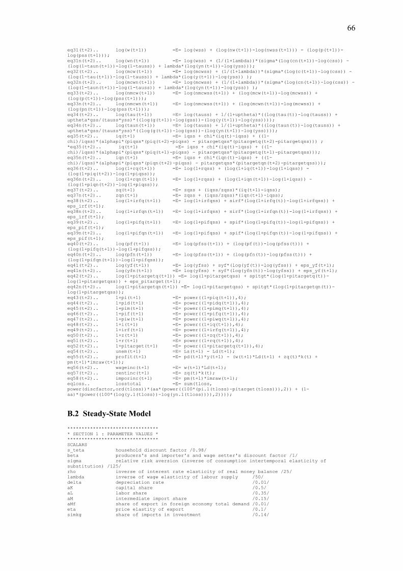
66
eq31(t+2).. log(w(t+1)) =E= log(wss) + (log(nw(t+1))-log(nwss(t+1))) - (log(p(t+1))-
log(pss(t+1)));
eq31n(t+2).. log(wn(t+1)) =E= log(wss) + (1/(1+lambda))*(sigma*(log(cn(t+1))-log(css)) -
(log(1-taun(t+1))-log(1-tauss)) + lambda*(log(yn(t+1))-log(yss)));
eq32(t+2).. log(mcw(t+1)) =E= log(mcwss) + (1/(1+lambda))*(sigma*(log(c(t+1))-log(css)) -
(log(1-tau(t+1))-log(1-tauss)) + lambda*(log(y(t+1))-log(yss)) );
eq32n(t+2).. log(mcwn(t+1)) =E= log(mcwss) + (1/(1+lambda))*(sigma*(log(cn(t+1))-log(css)) -
(log(1-taun(t+1))-log(1-tauss)) + lambda*(log(yn(t+1))-log(yss)) );
eq33(t+2).. log(nmcw(t+1)) =E= log(nmcwss(t+1)) + (log(mcw(t+1))-log(mcwss)) +
(log(p(t+1))-log(pss(t+1)));
eq33n(t+2).. log(nmcwn(t+1)) =E= log(nmcwss(t+1)) + (log(mcwn(t+1))-log(mcwss)) +
(log(pn(t+1))-log(pss(t+1)));
eq34(t+2).. log(tau(t+1)) =E= log(tauss) + 1/(1+uptheta)*((log(tau(t))-log(tauss)) +
uptheta*gss/(tauss*yss)*((log(g(t+1))-log(gss))-(log(y(t+1))-log(yss))));
eq34n(t+2).. log(taun(t+1)) =E= log(tauss) + 1/(1+uptheta)*((log(taun(t))-log(tauss)) +
uptheta*gss/(tauss*yss)*((log(g(t+1))-log(gss))-(log(yn(t+1))-log(yss))));
eq35(t+2).. iq(t+1) =E= iqss + chi*(iq(t)-iqss) + ((1-
chi)/iqss)*(alphapi*(piqss*(piq(t+2)-piqss) - pitargetqss*(pitargetq(t+2)-pitargetqss))) ;
*eq35(t+2).. iq(t+1) =E= iqss + chi*(iq(t)-iqss) + ((1-
chi)/iqss)*(alphapi*(piqss*(piq(t+1)-piqss) - pitargetqss*(pitargetq(t+1)-pitargetqss)));
eq35n(t+2).. iqn(t+1) =E= iqss + chi*(iqn(t)-iqss) + ((1-
chi)/iqss)*(alphapi*(piqss*(piqn(t+2)-piqss) - pitargetqss*(pitargetqn(t+2)-pitargetqss)));
eq36(t+2).. log(1+rq(t+1)) =E= log(1+rqss) + (log(1+iq(t+1))-log(1+iqss)) -
(log(1+piq(t+2))-log(1+piqss));
eq36n(t+2).. log(1+rqn(t+1)) =E= log(1+rqss) + (log(1+iqn(t+1))-log(1+iqss)) -
(log(1+piqn(t+2))-log(1+piqss));
eq37(t+2).. zq(t+1) =E= zqss + (iqss/zqss)*(iq(t+1)-iqss);
eq37n(t+2).. zqn(t+1) =E= zqss + (iqss/zqss)*(iqn(t+1)-iqss);
eq38(t+2).. log(1+irfq(t+1)) =E= log(1+irfqss) + sirf*(log(1+irfq(t))-log(1+irfqss)) +
eps_irf(t+1);
eq38n(t+2).. log(1+irfqn(t+1)) =E= log(1+irfqss) + sirf*(log(1+irfqn(t))-log(1+irfqss)) +
eps_irf(t+1);
eq39(t+2).. log(1+pifq(t+1)) =E= log(1+pifqss) + spif*(log(1+pifq(t))-log(1+pifqss)) +
eps_pif(t+1);
eq39n(t+2).. log(1+pifqn(t+1)) =E= log(1+pifqss) + spif*(log(1+pifqn(t))-log(1+pifqss)) +
eps_pif(t+1);
eq40(t+2).. log(pf(t+1)) =E= log(pfss(t+1)) + (log(pf(t))-log(pfss(t))) +
(log(1+pifq(t+1))-log(1+pifqss));
eq40n(t+2).. log(pfn(t+1)) =E= log(pfss(t+1)) + (log(pfn(t))-log(pfss(t))) +
(log(1+pifqn(t+1))-log(1+pifqss));
eq41(t+2).. log(yf(t+1)) =E= log(yfss) + syf*(log(yf(t))-log(yfss)) + eps_yf(t+1);
eq41n(t+2).. log(yfn(t+1)) =E= log(yfss) + syf*(log(yfn(t))-log(yfss)) + eps_yf(t+1);
eq42(t+2).. log(1+pitargetq(t+1)) =E= log(1+pitargetqss) + spitgt*(log(1+pitargetq(t))-
log(1+pitargetqss)) + eps_pitarget(t+1);
eq42n(t+2).. log(1+pitargetqn(t+1)) =E= log(1+pitargetqss) + spitgt*(log(1+pitargetqn(t))-
log(1+pitargetqss));
eq43(t+2).. 1+pi(t+1) =E= power((1+piq(t+1)),4);
eq44(t+2).. 1+pid(t+1) =E= power((1+pidq(t+1)),4);
eq45(t+2).. 1+pim(t+1) =E= power((1+pimq(t+1)),4);
eq46(t+2).. 1+pif(t+1) =E= power((1+pifq(t+1)),4);
eq47(t+2).. 1+piw(t+1) =E= power((1+piwq(t+1)),4);
eq48(t+2).. 1+i(t+1) =E= power((1+iq(t+1)),4);
eq49(t+2).. 1+irf(t+1) =E= power((1+irfq(t+1)),4);
eq50(t+2).. 1+z(t+1) =E= power((1+zq(t+1)),4);
eq51(t+2).. 1+r(t+1) =E= power((1+rq(t+1)),4);
eq52(t+2).. 1+pitarget(t+1) =E= power((1+pitargetq(t+1)),4);
eq54(t+2).. unem(t+1) =E= Ls(t+1) - Ld(t+1);
eq55(t+2).. profit(t+1) =E= pd(t+1)*y(t+1) - (w(t+1)*Ld(t+1) + zq(t)*k(t) +
pm(t+1)*imraw(t+1));
eq56(t+2).. wageinc(t+1) =E= w(t+1)*Ld(t+1);
eq57(t+2).. rentinc(t+1) =E= zq(t)*k(t);
eq58(t+2).. imporinc(t+1) =E= pm(t+1)*imraw(t+1);
eqloss.. losstotal =E= sum(tloss,
power(discfactor,ord(tloss))*(aa*(power((100*(pi.l(tloss)-pitarget(tloss))),2)) + (1-
aa)*(power((100*(log(y.l(tloss))-log(yn.l(tloss)))),2))));
B.2 Steady-State Model ********************************
* SECTION 1 : PARAMETER VALUES *
********************************
SCALARS
s_teta household discount factor /0.98/
beta producers's and importer's and wage setter's discount factor /1/
sigma relative risk aversion (inverse of consumption intertemporal elasticity of
substitution) /125/
rho inverse of interest rate elasticity of real money balance /25/
lambda inverse of wage elasticity of labour supply /50/
delta depreciation rate /0.01/
aK capital share /0.5/
aL labor share /0.35/
aM intermediate import share /0.15/
aMf share of export in foreign economy total demand /0.01/
eta price elastity of export /0.1/
simkg share of imports in investment /0.14/
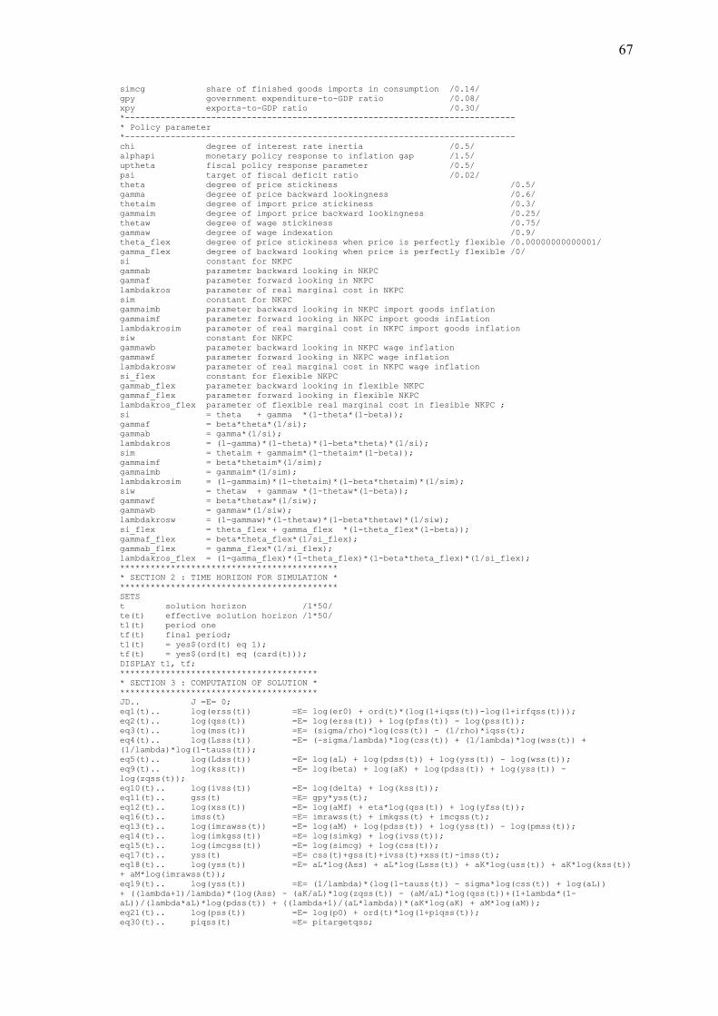
67
simcg share of finished goods imports in consumption /0.14/
gpy government expenditure-to-GDP ratio /0.08/
xpy exports-to-GDP ratio /0.30/
*-----------------------------------------------------------------------------
* Policy parameter
*-----------------------------------------------------------------------------
chi degree of interest rate inertia /0.5/
alphapi monetary policy response to inflation gap /1.5/
uptheta fiscal policy response parameter /0.5/
psi target of fiscal deficit ratio /0.02/
theta degree of price stickiness /0.5/
gamma degree of price backward lookingness /0.6/
thetaim degree of import price stickiness /0.3/
gammaim degree of import price backward lookingness /0.25/
thetaw degree of wage stickiness /0.75/
gammaw degree of wage indexation /0.9/
theta_flex degree of price stickiness when price is perfectly flexible /0.00000000000001/
gamma_flex degree of backward looking when price is perfectly flexible /0/
si constant for NKPC
gammab parameter backward looking in NKPC
gammaf parameter forward looking in NKPC
lambdakros parameter of real marginal cost in NKPC
sim constant for NKPC
gammaimb parameter backward looking in NKPC import goods inflation
gammaimf parameter forward looking in NKPC import goods inflation
lambdakrosim parameter of real marginal cost in NKPC import goods inflation
siw constant for NKPC
gammawb parameter backward looking in NKPC wage inflation
gammawf parameter forward looking in NKPC wage inflation
lambdakrosw parameter of real marginal cost in NKPC wage inflation
si_flex constant for flexible NKPC
gammab_flex parameter backward looking in flexible NKPC
gammaf_flex parameter forward looking in flexible NKPC
lambdakros_flex parameter of flexible real marginal cost in flesible NKPC ;
si = theta + gamma *(1-theta*(1-beta));
gammaf = beta*theta*(1/si);
gammab = gamma*(1/si);
lambdakros = (1-gamma)*(1-theta)*(1-beta*theta)*(1/si);
sim = thetaim + gammaim*(1-thetaim*(1-beta));
gammaimf = beta*thetaim*(1/sim);
gammaimb = gammaim*(1/sim);
lambdakrosim = (1-gammaim)*(1-thetaim)*(1-beta*thetaim)*(1/sim);
siw = thetaw + gammaw *(1-thetaw*(1-beta));
gammawf = beta*thetaw*(1/siw);
gammawb = gammaw*(1/siw);
lambdakrosw = (1-gammaw)*(1-thetaw)*(1-beta*thetaw)*(1/siw);
si_flex = theta_flex + gamma_flex *(1-theta_flex*(1-beta));
gammaf_flex = beta*theta_flex*(1/si_flex);
gammab_flex = gamma_flex*(1/si_flex);
lambdakros_flex = (1-gamma_flex)*(1-theta_flex)*(1-beta*theta_flex)*(1/si_flex);
*******************************************
* SECTION 2 : TIME HORIZON FOR SIMULATION *
*******************************************
SETS
t solution horizon /1*50/
te(t) effective solution horizon /1*50/
t1(t) period one
tf(t) final period;
t1(t) = yes$(ord(t) eq 1);
tf(t) = yes$(ord(t) eq (card(t)));
DISPLAY t1, tf;
***************************************
* SECTION 3 : COMPUTATION OF SOLUTION *
***************************************
JD.. J =E= 0;
eq1(t).. log(erss(t)) =E= log(er0) + ord(t)*(log(1+iqss(t))-log(1+irfqss(t)));
eq2(t).. log(qss(t)) =E= log(erss(t)) + log(pfss(t)) - log(pss(t));
eq3(t).. log(mss(t)) =E= (sigma/rho)*log(css(t)) - (1/rho)*iqss(t);
eq4(t).. log(Lsss(t)) =E= (-sigma/lambda)*log(css(t)) + (1/lambda)*log(wss(t)) +
(1/lambda)*log(1-tauss(t));
eq5(t).. log(Ldss(t)) =E= log(aL) + log(pdss(t)) + log(yss(t)) - log(wss(t));
eq9(t).. log(kss(t)) =E= log(beta) + log(aK) + log(pdss(t)) + log(yss(t)) -
log(zqss(t));
eq10(t).. log(ivss(t)) =E= log(delta) + log(kss(t));
eq11(t).. gss(t) =E= gpy*yss(t);
eq12(t).. log(xss(t)) =E= log(aMf) + eta*log(qss(t)) + log(yfss(t));
eq16(t).. imss(t) =E= imrawss(t) + imkgss(t) + imcgss(t);
eq13(t).. log(imrawss(t)) =E= log(aM) + log(pdss(t)) + log(yss(t)) - log(pmss(t));
eq14(t).. log(imkgss(t)) =E= log(simkg) + log(ivss(t));
eq15(t).. log(imcgss(t)) =E= log(simcg) + log(css(t));
eq17(t).. yss(t) =E= css(t)+gss(t)+ivss(t)+xss(t)-imss(t);
eq18(t).. log(yss(t)) =E= aL*log(Ass) + aL*log(Lsss(t)) + aK*log(uss(t)) + aK*log(kss(t))
+ aM*log(imrawss(t));
eq19(t).. log(yss(t)) =E= (1/lambda)*(log(1-tauss(t)) - sigma*log(css(t)) + log(aL))
+ ((lambda+1)/lambda)*(log(Ass) - (aK/aL)*log(zqss(t)) - (aM/aL)*log(qss(t))+(1+lambda*(1-
aL))/(lambda*aL)*log(pdss(t)) + ((lambda+1)/(aL*lambda))*(aK*log(aK) + aM*log(aM));
eq21(t).. log(pss(t)) =E= log(p0) + ord(t)*log(1+piqss(t));
eq30(t).. piqss(t) =E= pitargetqss;

68
eq31(t).. piqss(t) =E= (1-simcg)*pidqss(t) + simcg*pimqss(t);
eq32(t).. log(npdss(t)) =E= log(p0) + ord(t)*log(1+pidqss(t));
eq33(t).. log(pdss(t)) =E= log(npdss(t)) - log(pss(t));
eq7(t).. log(mcdss(t)) =E= aL*log(wss(t))+aK*log(zqss(t))+aM*log(pmss(t))-aL*log(Ass)-
aL*log(aL)-aK*log(aK)-aM*log(aM);
eq8(t).. log(nmcdss(t)) =E= log(mcdss(t)) + log(pss(t));
eq22(t).. log(pmss(t)) =E= log(qss(t));
eq23(t).. npmss(t) =E= pmss(t)*pss(t);
eq24(t).. log(1+pimqss(t)) =E= (1/ord(t))*(log(npmss(t))-log(p0));
eq24a(t).. log(1+pimqss(t)) =E= (1/ord(t))*(log(nmcmss(t))-log(p0*mcmss('1')));
eq7m(t).. log(mcmss(t)) =E= log(qss(t));
eq8m(t).. log(nmcmss(t)) =E= log(mcmss(t)) + log(pss(t));
eq6(t).. log(wss(t)) =E= (1/(1+lambda))*(sigma*log(css(t)) - log(1-tauss(t)) +
lambda*log(pdss(t)) + lambda*log(yss(t)) + lambda*log(aL));
eq37(t).. nwss(t) =E= wss(t)*pss(t);
eq38(t).. log(1+piwqss(t)) =E= (1/ord(t))*(log(nwss(t))-log(p0*wss('1')));
eq38a(t).. log(1+piwqss(t)) =E= (1/ord(t))*(log(nmcwss(t))-log(p0*mcwss('1')));
eq7w(t).. log(mcwss(t)) =E= (1/(1+lambda))*(sigma*log(css(t)) - log(1-tauss(t)) +
lambda*log(pdss(t)) + lambda*log(yss(t)) + lambda*log(aL));
eq8w(t).. log(nmcwss(t)) =E= log(mcwss(t)) + log(pss(t));
eq25(t).. log(pfss(t)) =E= log(p0) + ord(t)*log(1+pifqss(t));
eq26(t).. 1+irfss(t) =E= (1+rfss(t))*(1+pifss(t));
eq27(t).. 1+iss(t) =E= (1+rss(t))*(1+piss(t));
eq28(t).. zqss(t) =E= iqss(t)+delta;
*eq28(t).. zss(t) =E= iss(t)+(power((1+delta),4)-1);
eq29(t).. tauss(t) =E= gss(t)/yss(t)-psi;
eq34(t).. rss(t) =E= 1/s_teta-1;
eq35(t).. rfss(t) =E= rss(t);
eq36(t).. log(yfss(t)) =E= log(xpy)+log(yss(t))-log(aMf)-eta*log(qss(t));
eq39(t).. uss(t) =E= 1;
eq40(t).. 1+piss(t) =E= power((1+piqss(t)),4);
eq41(t).. 1+pidss(t) =E= power((1+pidqss(t)),4);
eq42(t).. 1+pimss(t) =E= power((1+pimqss(t)),4);
eq43(t).. 1+pifqss(t) =E= sqrt(sqrt(1+pifss(t)));
eq44(t).. 1+piwss(t) =E= power((1+piwqss(t)),4);
eq45(t).. 1+iqss(t) =E= sqrt(sqrt(1+iss(t)));
eq46(t).. 1+irfqss(t) =E= sqrt(sqrt(1+irfss(t)));
*eq47(t).. 1+zqss(t) =E= sqrt(sqrt(1+zss(t)));
eq47(t).. 1+zss(t) =E= power((1+zqss(t)),4);
eq48(t).. 1+rqss(t) =E= sqrt(sqrt(1+rss(t)));
eq49(t).. 1+rfqss(t) =E= sqrt(sqrt(1+rfss(t)));
eq50.. 1+pitargetqss =E= sqrt(sqrt(1+pitargetss));

Chapter 3
Monetary transmission of persistent shock to the risk
premium: the case of Indonesia
70
3.1 Introduction
Adverse exchange rate shocks frequently hit Indonesia. Such particular shocks might
occur in terms of frequent one time shocks or in a more persistent way during a longer
period. The currency crisis that badly hit the country in 1997-1998 can be considered as
a severe persistent shock to the risk premium that devalued the exchange rate and
altered the economy‘s dynamic equilibrium. Invaluable lesson should be continuously
learned to pursue better monetary management in anticipating possible recurrence of
such crises. Better understanding of monetary transmission mechanism and its
consequence to monetary policy limitation is therefore necessary and worthwhile.
Cost channel of monetary policy has been increasingly explored for the case of
developed economies. Barth and Ramey (2001) provide empirical evidence for cost
channel of monetary policy based on industry level data. Ravenna and Walsh (2006)
shows that, if nominal interest rate adjustment directly affect real marginal cost, then
interest rate policy directly affects inflation. They also show that any shock to the
economy with the presence of the channel will generate a trade-off between stabilizing
inflation and stabilizing output gap. Chowdhury, et al. (2006) applied a structural
approach to find that the estimated direct cost effects of short-run nominal interest rates
significantly contribute to the inflation dynamics in the majority of G7 countries.
Existing empirical studies on Indonesia‘s monetary transmission compiled in
Warjiyo and Juda Agung (2002) did not include cost channel of interest rate. However,
the study, which employed VAR method, found ―price puzzle‖ in response to monetary
policy tightening. This phenomenon is usually linked to either VAR misspecification or
the possible existence of a strong cost channel of monetary policy. As an emerging
economy with relatively low labour productivity, it is likely that capital accumulation
has been the main source of Indonesia‘s output growth. Hossain (2006) estimated a
71
Cobb-Douglas production function to find that capital accumulation accounts for 60
percent source of growth in Indonesia for the last forty years. It is in the spirit of the
Young (1992) paper that claimed that growth in East Asian countries was mainly driven
by high rates of capital formation. Combined with higher lending rate and lower wage
than those in advanced economy, one can argue that capital share (capital owner‘s
income as a fraction of GDP) is greater than the labour share. This argument enhances
the importance of investigating cost channel of monetary policy.
This study uses a new Keynesian dynamic general equilibrium model of a small
open economy involving four domestic economic players, namely the household, the
firm-producer, the government, and the central bank, which interact with the foreign
economy. The model characterizes the household‘s money-in-the-utility function and
the firm‘s constant elasticity substitution production that employs labour, capital goods,
and domestic and imported raw material. Interest rate policy is transmitted to the new
Keynesian Phillips curve type of inflation through channels of aggregate demand,
exchange rate pass-through, and cost of capital. I assume that the expectation channel of
monetary policy is fully credible. It corresponds to agent‘s rational price expectation
and perfectly credible monetary authority, which utilizes a simple interest rate policy
rule contingent to the state of shock. Shock to interest rate risk premium is applied
through a covered interest rate parity determination of exchange rate. The model is
adapted and developed from optimizing models with staggered wage and prices-setting,
which have been widely used in the literature on inflation and monetary policy10
.
The model is employed to observe the effect of short term persistent shock to the
risk premium on the performance of an economy, which is intended to be close to the
structure and behaviour of Indonesia‘s economy. The focus of this study are the relative
10
See, for example, Ravenna and Walsh (2006), Christiano et al. (2005), Smets and Wouters (2003),
Erceg and Levin (2003), Woodford (2003), and Murchison (2004). The first two incorporated interest
cost channel for monetary policy.
72
importance of monetary transmission channel that pass the shock and interest rate
response to inflation and how monetary policy should respond optimally to the
particular type and state of the shocks, given the distinctive monetary transmission.
This paper shows that nominal exchange rate depreciation triggered by persistent
shocks to interest risk premium worsens the state of the economy in the short- and long-
run. The shocks are transmitted through the economy characterizing lack of response of
consumer price disinflation to monetary policy contraction resulted from high real
rigidity, strong cost channel of interest rate, strong cost channel of exchange rate pass-
through, weak demand-side channel of exchange rate pass-through, and weak aggregate
supply channel of interest rate.
The study suggests a proper monetary policy response, which is the smallest
interest rate increases within the feasible set of monetary policy responses that the
model recommends, to minimize the adverse effects of the shocks. Other economic
policies might be necessarily complementary to the limited span of monetary policy that
can in turn help strengthening aggregate demand channel of interest rate. The most
important one is policies that help reducing capital share of economy‘s output and
consecutively could weaken the cost channel of interest rate.
The organization of the rest of this paper is as follows. Section 3.2 presents a
dynamic equilibrium model with prices and wage stickiness. Section 3.3 presents
simulation scenarios, parameter calibration and model solution. Section 3.4 analyses
simulation result. Section 3.5 concludes the study and infers some policy
recommendations.
3.2 The model
This study extends the dynamic general equilibrium model used in chapter 2. I extend
the model by incorporating interest-rate risk premium on foreign-denominated asset as a
73
function of ratio of net foreign debt to GDP. Then, balance of payment block is
developed that results in equations of current account, capital account, trade and service
account, and net foreign asset. Moreover, I assume that the government also collects
income tax on capital goods lessor‘s and the firm owner‘s dividend in addition to wage
income tax in the previous model. I also change the Cobb-Douglas production
technology with a constant elasticity of substitution technology to allow lower
elasticities of factor inputs‘ demand with respect to input prices. The model‘s extension
is described as follows.
3.2.1 The household
The dynamic budget constraint is expressed in domestic currency‘s nominal and real
terms as follows.
))(1(
~))1((
11
*
1
*
111
1
*
11
*
11
ttttttttt
m
t
H
ttt
HG
tt
ttt
H
tt
H
tt
HG
t
HG
t
d
t
d
ttt
PkPzlWimPBsiBi
kkPBsBsBBMMcP
(1.1)
ttttttt
m
t
H
ttt
HG
tt
d
t
t
t
tt
H
tt
H
tt
HG
t
HG
t
d
t
d
tt
kzlwimpbqrbrm
kkbqbqbbmmc
11
*
11
*
1111
1
*
11
*
11
)1(~
1
))1(()()()(
(1.2)
Sources of household‘s revenues are income from supplying labour services
(wages), selling imported goods, renting capital goods to the firm, owning firm
(dividend) and selling the previous period‘s depreciated capital goods, as well as
interest income on government bonds and foreign assets.
I assume that the household‘s net foreign asset position is negative )0(*
HtB ,
meaning that the household is a net debtor of foreign asset. I further assume that foreign
investors require a risk premium, t , for the rate of interest, *~
ti , of foreign currency-
denominated loans they extend to the domestic household, so that
74
)1)(1()~
1(**
ttt ii . Hence the principal and interest income from foreign asset is
0)1)(1(*11
*1
Htttt Bsi .
I follow Al-Eyd and Hall (2006), Murchison, et. al (2004), and Schmitt-Grohe and
Uribe (2003) in defining the country-specific risk premium, t , which depends on net
foreign debt-to-GDP ratio. The risk premium is also subject to a shock process, t ,
representing unforecastable changes in foreign investor‘s preferences on domestic
assets.
t
yP
Bs
ttt
tt
e
1
*
, (1.3)
where is scaling parameter. The equation says that foreign asset interest-rate risk
premium depends on net foreign debt, exchange rate, output, and exogenous shock to
the risk premium. An increase in net foreign debt (or a decrease in net foreign asset)
negatively affects the ability of domestic resident to repay the debt. Exchange rate
depreciation increases the amount of domestic currency required to pay foreign debt
and, in turn, worsens domestic resident‘s ability to repay their foreign debt. A declining
real income worsens the economy‘s capability for foreign debt repayment. Risk
premium on the foreign debt is absent when foreign asset equals foreign debt and
negative if net foreign asset is positive. The later means that the domestic household can
enjoy a lower-than-world interest rate for its foreign debt.
From the maximization of household utility function with respect to labour supply and
consumption, we can find the real marginal cost of working of the form
1
1
)1(
1
)(
t
tLttwt
ycAmc (1.4)
75
The household rents out capital goods to the firm with real rental rate of capital, tz ,
which is obtained by combining the first order condition of utility maximization with
respect to real capital stock and nominal domestic bonds as follow
11
tt
tt
E
rz
(1.5)
Real rental price of capital that the household-lessor charges to the firm should cover
real interest rate, depreciation rate of capital and the expected future income tax rate.
Real marginal cost of imports equals real import price equation when prices are fully
flexible, which is equal to real exchange rate.
t
m
t qmc (1.6)
Nominal exchange rate is obtained by combining the first order condition of the
household‘s utility maximization with respect to nominal domestic and foreign bonds,
which implies covered interest rate parity.
)1(1
1*
1 t
t
tttt
i
isEs
(1.7)
In order to obtain the household‘s financial assets and financial account, we can
elaborate the equality of nominal budget constraint (1.2) by substituting the firm‘s real
profit )( 11 tttmttttt kzimplwy , capital accumulation equation,
])1([ 1 ttt ivkk , and the decomposition of real investment as domestic and
imported capital goods )(kgt
dtt imiviv . We can further substitute the decomposition
of imported goods as finished goods, intermediate goods and capital goods
)(kgt
cgt
rmtt imimimim , and take into account that domestic output, ty , is supplied
to the domestic household as consumption goods (dtc ), to the firm as additional capital
76
goods (dtiv ), to the government as consumption and investment goods ( tg ), and to the
foreign importers as exported goods ( tx ). These substitutions result in the household‘s
dynamic real budget constraint that can be rearranged to get the household‘s real
financial assets of the form
t
dtd
tttHtttt
HGtttttt
Ht
mmybqrbrgimqxb
1])1)(1()1[()( 1*
11*
111 (1.8)
where Htb is the household‘s real financial investment on the government bonds and
foreign bonds in period t. It is equal to their net real revenues as exporter and importer
and as the supplier of goods to the government, plus the principal and interest real
income from the previous period‘s financial investment, minus real income tax
expenditure and changes in real money holding.
3.2.2 The firm-producer
The firm produces output using a Constant Elasticity of Substitution (CES) production
technology that utilizes labour, capital, and foreign and domestically produced
intermediate goods as production input. The aggregate real output of the economy
follows Murchison et al. (2004) to take the form
111
1
1
11
1
)()()(
rmtMttK
dttLt imkulAy (2.1)
where MKL ,, are labour, capital and import share, respectively, which are assumed
to be constant and forms a constant return-to-scale technology of production, and is
the elasticity of substitution between factor inputs. The objective of the firm is to choose
the level of factor inputs that maximize its present discounted values of lifetime real
profit, which is the deviation of total real revenues from total real cost.
77
11
111
1
1
11
1
)()()(
tt
rmt
mt
dtt
rmtMttK
dttLt kzimplwimkulA
(2.2)
Employment equation is given by the first order condition with respect to labour
demand
t
ttLdt
w
yAl
1
(2.3)
From the first order condition of the firm‘s profit maximization, we can obtain the
demand for the imported intermediate goods of the form
mt
tMrmt
p
yim (2.4)
The firm‘s stock of capital goods required for production is obtained from the first order
condition of the firm‘s profit maximization with respect to capital:
t
ttttKt
z
yEuEk 1
11
(2.5)
Real marginal cost of producing goods is derived from the firm‘s real cost minimization
problem in which the aggregate firm chooses the level of factors inputs that minimize
total real cost, 11 ttrmt
mtttt kzimplwtc , subject to CES production function (2.1).
The aggregate firm‘s real marginal cost, dtmc , is expressed as a function of real wage,
real rental price of capital, real import price and the level of technology of the form:
1
1
11
1
1
1
1
111
mt
M
t
tK
t
t
LLt
tdt
pz
u
A
w
A
wmc (2.6)
78
3.2.3 The fiscal authority
Government expenditure is financed through collecting income tax on the importer‘s,
capital goods lessor‘s, and firm owner‘s dividend or issuing domestic- and foreign-
denominated bonds. The government‘s nominal dynamic budget constraint is expressed
as
ttGtttt
GHtt
st
stttt
Gtt
GHt gPBsiBiMMyPBsB
*11
*1111
*)1)(1()1( (3.1)
where *G
ttGHt
Gt BsBB is government revenue from issuing domestic bonds (
GHtB )
and foreign bond (*G
tB ), ttt yP is tax revenue, )( 1st
st MM is seignorage revenue, tg
is real government spending, and ts is nominal exchange rate. The government real
debt, which comprises its debt to the household and to the foreign economy,
*Gtt
GHt
Gt bqbb , takes the form
t
sts
ttttGttt
GHttt
Gt
mmyqbrbrgb
1)1)(1()1( 1*
11*
111
(3.2)
3.2.4 Real net foreign debt and financial account
Real net foreign debt, *td , is obtained from the household‘s and the government‘s real
budget constraints. It is used to finance trade deficit and repay the previous period‘s
foreign debt.
*11
*1
*)1)(1()/( ttttttt drqximd (4.1)
Financial account (foreign debt flow), tFA , is the total of changes in the government‘s
net foreign debt and changes in the private sector‘s net foreign debt. We can get the
national debt flow from the household and the government‘s nominal budget constraints
by assuming that government‘s domestic debt equals the household‘s holding on
79
government bonds )(HGt
GHt BB , that foreign residents do not hold government
domestic-denominated bond, and the equilibrium of money holds.
*11
*1
*]1)1)(1[(/ ttttttttt BisxPimPFA (4.2)
3.2.5 The goods market equilibrium
The equilibrium of goods market is defined by resource constraint that equate the
aggregate demand for output with the aggregate supply of output (2.1) of the form
111
1
1
11
1
)()()(
rmtMttK
dttLttttt imkulAimxivgc
(5)
3.3 Simulation Scenario and Parameter Setting
I conduct a simulation by applying an eight-quarter one percentage point positive
exogenous shocks to the risk premium equation11
. The type, magnitude and length of
shock are meant to resemble a moderate currency crisis. The simulation objective is to
evaluate the effect of such shocks on economic performance, in particular the exchange
rate, balance of payment and monetary policy response. By applying one single type of
shock, it is implicitly assumed that other kinds of shocks are not present and the
economy is not pursuing disinflation. I also conduct a one-time exogenous shock to
interest rate policy in order to confirm how the channel of monetary transmission
works.
Table 3.1 exhibits parameter calibration. The firm‘s, importer‘s and wage setter‘s future
profits are discounted at discount factor 99.0 . From consumption Euler equation,
we get the steady-state real interest rate that equals the household's rate of time
preference. Setting real interest rate at 0.02 corresponds to the household discount
11
Steady-state values and the simulation paths are solved by using GAMS software that employ the
Generalized Reduced Gradient method of solution for non-linear programming problems (Rosenthal
(2006), Drud (2006))
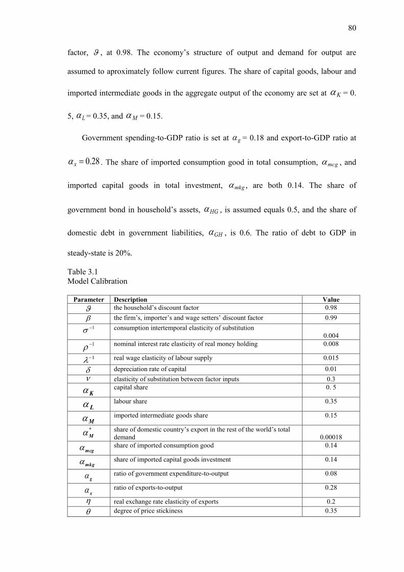
80
factor, , at 0.98. The economy‘s structure of output and demand for output are
assumed to aproximately follow current figures. The share of capital goods, labour and
imported intermediate goods in the aggregate output of the economy are set at K = 0.
5, L = 0.35, and M = 0.15.
Government spending-to-GDP ratio is set at g = 0.18 and export-to-GDP ratio at
28.0x . The share of imported consumption good in total consumption, mcg , and
imported capital goods in total investment, mkg , are both 0.14. The share of
government bond in household‘s assets, HG , is assumed equals 0.5, and the share of
domestic debt in government liabilities, GH , is 0.6. The ratio of debt to GDP in
steady-state is 20%.
Table 3.1
Model Calibration
Parameter Description Value
the household‘s discount factor 0.98
the firm‘s, importer‘s and wage setters‘ discount factor 0.99
1 consumption intertemporal elasticity of substitution
0.004
1 nominal interest rate elasticity of real money holding 0.008
1 real wage elasticity of labour supply 0.015
depreciation rate of capital 0.01
elasticity of substitution between factor inputs 0.3
K capital share 0. 5
L labour share 0.35
M imported intermediate goods share 0.15
*
M share of domestic country‘s export in the rest of the world‘s total
demand
0.00018
mcg share of imported consumption good 0.14
mkg share of imported capital goods investment 0.14
g ratio of government expenditure-to-output 0.08
x ratio of exports-to-output 0.28
real exchange rate elasticity of exports 0.2
degree of price stickiness 0.35
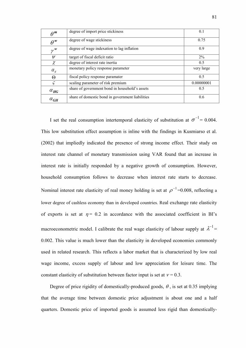
81
m degree of import price stickiness 0.1
w degree of wage stickiness 0.75
w degree of wage indexation to lag inflation 0.9
target of fiscal deficit ratio 2%
degree of interest rate inertia 0.5
monetary policy response parameter very large
fiscal policy response paramater 0.5
scaling parameter of risk premium 0.00000001
HG share of government bond in household‘s assets 0.5
GH share of domestic bond in government liabilities 0.6
I set the real consumption intertemporal elasticity of substitution at 1 = 0.004.
This low substitution effect assumption is inline with the findings in Kusmiarso et al.
(2002) that impliedly indicated the presence of strong income effect. Their study on
interest rate channel of monetary transmission using VAR found that an increase in
interest rate is initially responded by a negative growth of consumption. However,
household consumption follows to decrease when interest rate starts to decrease.
Nominal interest rate elasticity of real money holding is set at 1 =0.008, reflecting a
lower degree of cashless economy than in developed countries. Real exchange rate elasticity
of exports is set at = 0.2 in accordance with the associated coefficient in BI‘s
macroeconometric model. I calibrate the real wage elasticity of labour supply at 1 =
0.002. This value is much lower than the elasticity in developed economies commonly
used in related research. This reflects a labor market that is characterized by low real
wage income, excess supply of labour and low appreciation for leisure time. The
constant elasticity of substitution between factor input is set at = 0.3.
Degree of price rigidity of domestically-produced goods, , is set at 0.35 implying
that the average time between domestic price adjustment is about one and a half
quarters. Domestic price of imported goods is assumed less rigid than domestically-
82
produced goods (m
= 0.1), implying that the average duration of import price is 3.3
months. In setting rigidity parameter, I refer to business price setting survey for
Indonesia‘s economy in Darsono et al. (2002), which found that manufacturing goods
prices stay an average of 4.6 months and that exchange rate changes is passed-through
to import price in the same quarter. Wage rigidity is assumed at w
= 0.75,
corresponding to yearly nominal wage changes. However, the refference for wage
changes is heavily based on the previous wage inflation rather than on forward looking
optimal price setting. This behaviour is reflected in parameter w
that is equal to 0.9.
Inflation feedback parameter in the simple interest rate rule is set at a value that
minimizes present discounted value of dynamic welfare loss over a hundred quarters
after the shock. The loss function is symmetric of the form
0
22)()(
s
ststs
Lt yyEL , where monetary policy makers have equal
preferences on both inflation and output stabilization. Inflation feedback coefficient is
contingent on the magnitude and extent of a shock to the risk premium. I search the
optimal policy feedback coefficient by fixing interest rate smoothing coefficient at
5.0 , reflecting equally backward- and forward-looking behaviour of monetary
authority in formulating interest rate policy. Figure 3.1 shows the range of feasible
inflation feedback parameters when interest rate responds to a future period‘s inflation
gap. The figures show that the feasible set of the monetary authority response to the risk
premium shock is a rising interest rate. However, the optimal response, which produces
the lowest inflation effect and the smallest short-run output contraction, is the smallest
interest rate increases within the feasible set. The highest interest rate increase in the set
corresponds to the most nonoptimal response.
83
3.4 Simulation Results
3.4.1 Exchange rate and balance of payment
Figure 3.2 exhibit the responses economic variables to an eight-quarter one percentage
point shock to the risk premium. Nominal exchange rate contemporaneously depreciates
as a response to risk premium shock, but its extent is lowered by immediate interest rate
response. The rate of nominal exchange finally achieves a new, weaker steady-state
level when the nominal rate of interest returns to and stabilizes at the initial rate, leaving
expectation channel works solely. The long run equilibrium of nominal exchange rate
becomes weaker to compensate a lower relative price of foreign to domestic goods so
that real exchange rate is unchanged in the long run.
Real export follows real exchange rate movement in the absence of changes to
foreign demand. With a low elasticity of real export with respect to real exchange rate,
real export only moves up by about 0.027%. It then falls below initial steady-state when
real exchange rate strengthens several quarters after the shock. Exports returns to its
initial steady-state level in the long run.
Following an increase in real import price, real import falls by about 1.6%, much
larger than an increase in real exports in the early period of shocks. Foreign price value
of imports declines sharply since foreign price quarterly inflation stays the same. On the
other side, foreign price value of exported goods also declines accordingly as nominal
exchange rate depreciates more than an increase in real export and consumer price. The
net effect is a huge jump in trade surplus, exhibiting an inverted J-curve phenomenon.
Indonesia‘s trade surplus and real exports and imports in the period of currency crisis
justify the simulation result, to some extent, in terms of direction of related variables.
Figure 3.3 shows that in the aftermath of currency crisis in 1998, when nominal
84
exchange rate depreciated by 123%, real exports expanded 11.2% and real imports
contracted 2.9%, resulted in 83% trade surplus increases.
This result is in line with an empirical study on J-curve effect. Using a VECM
model on the quarterly data of Indonesia and its trading partners, Husman (2005)
concluded that J-curve phenomenon is not found in aggregate level data. It is only found
in the case of bilateral trade account with Japan, South Korea and Germany.
The movement of output, real import price and consumer inflation influence the
following cyclical pattern of trade account. Real import rebounds as aggregate demand
and output recovered and real import price lessens, resulting in a higher foreign price
value of imports. Conversely, external demand for domestic goods decreases due to real
exchange rate appreciation leading to a lower foreign price value of exports. Trade
surplus is lower than its initial level in the medium run and finally stabilizes in the long-
run at a slightly lower level than the initial steady-state value.
Some factors affect trade surplus dynamic. Exchange rate depreciation affects the
volume of imports more than that of export since import price is less rigid than domestic
price of exported goods. Moreover, imports plunge by significantly more than an
upsurge of export in the short-run owing to quite high import content in production
structure. In addition, real import price elasticity of imports is higher than real exchange
rate elasticity of exports so that the sum of the elasticity is less than unity. The last
factor explains why Marshall-Lerner condition does not hold. Hence the shock to the
risk premium could worsen trade balance in the long term. Unlike this model
simulation‘s result, Husman (2005) suggested that Marshall-Lerner condition is
satisfied in the overall sample, implying the Rupiah‘s depreciation will increase the
Indonesia exports in the long-run. She further found that although Marshal-Lerner
condition is satisfied, exchange rate elasticity of bilateral trade account is quite small.
85
One percentage change of real exchange rate only increases export to import ratio by
0.37%. Different finding regarding Marshall-Lerner condition might imply an
overestimated price elasticity of imports or underestimated price elasticity of exports
assumed in this study.
Short-run improvement of trade account surplus enables the economy to reduce its
net foreign debt. Afterwards, as trade account surplus worsens in the medium run and at
last stabilises below its initial steady-state level, the economy has to increase net foreign
debt continuously in the long-run. In line with net foreign debt‘s dynamics, service
account deficit improves in the short-run then is getting worse in the long-run, diverging
from the initial steady-state level. Overall, deficit current account lessens in the short-
run because a better trade account surplus is enhanced by a smaller service account
deficit. Ultimately, current account deficit becomes stable in the long-run at a worse
level. Financial account surplus decreases in the short-run, then increases in the
medium-run and finally reaches a higher steady-state surplus in the long-run.
3.4.2 Demand for and supply of input and output
Aggregate demand channel of interest rate policy works through exports, consumption
and investment. Consumption drops off contemporaneously as the expected lower
future consumption outweighs a small decrease in current real interest rate. It further
decreases in several more periods as real interest rate increases in the following periods.
When real interest rate stabilises in the long-run at a lower level than the initial steady-
state, consumption stabilises at a higher new steady-state.
Demand for the stock of capital goods, to be utilized in the next period, falls when
the shock to the risk premium hits the economy. Expected weakened aggregate demand
in the following periods is behind the firm decision to ration its capital stock. This is
often called as firm‘s balance sheet channel of interest rate to aggregate demand. A
86
stronger external demand for domestic goods and domestic demand for domestic
intermediate and final goods dampen investment demand contraction. The net effect is a
fall in aggregate demand for domestic output in the wake of the shock. Thus, exchange
rate depreciation triggered by a temporary shock to the risk premium is contractionary
to output.
Demand for other factor inputs drops as well. As import price is less rigid, a
depreciated real exchange rate leads to a more expensive real import price. Combined
with a contemporaneous lowered aggregate demand, this strongly discourages demand
for imported intermediate goods.
Employment falls because it is more affected by a much weakened aggregate
demand than by a slightly more inexpensive real wage. This result is caused by unitary
elasticity of labour demand with respect to real output and low elasticity of labour
supply with respect to real wage.
3.4.3 Costs, Prices and Inflations
A squeezed labour demand brings downward pressure on real marginal cost of working.
On the other side, leisure also decreases as demand for consumption goes down hence
labour supply increases and puts a downward pressure on real marginal cost of working.
Since nominal wage is quite rigid and highly indexed to its past inflation nominal wage
is not responsive to changes in real marginal cost of working resulted from immediate
adjustment in consumption and output.
Real wage declines because output price goes up and is more flexible than wage.
Therefore, the immediate domestic inflation response to a lower aggregate demand is
decreasing. In the following period of shock, investment starts to increase and
consumption get stronger, causing upward pressure to the real marginal cost of working
and wage inflation. Real wage is still below the initial steady-state level temporarily due
87
to a more flexible output price than wage. Therefore, throughout the rest of shocks
period the response of domestic inflation to a higher aggregate demand is decreasing.
Low real wage rigidity resulted from high nominal wage rigidity and low prices
rigidity can be linked to a high real rigidity. Romer (2006) defines real rigidity as a low
willingness of individual firm to change their relative price in response to changes in
real output resulting from variations in real aggregate demand. A larger real rigidity
corresponds to a greater consideration on competitor prices in price-setting behaviour. It
means that when real rigidity is high each firm wants its price to move more closely
with other prices. Bank Indonesia‘s business price setting survey (Darsono et al., 2002)
revealed that cost-based approach is the most widely adopted price setting strategies
among manufacturing and trading companies. The finding can justify the presence of
price rigidities. It reflects the firm‘s reluctance to change prices when no cost changes
occur. The survey also found that ‗cost plus variable profit margin‘ and ‗competitor
prices‘ are the next most price setting methods used in manufacturing and retail firms,
while ‗market condition‘ is not the important factor in price setting policy. The survey
results can be interpreted as low price rigidity in response to changes in cost and
changes in competitor price. The latter means a high real rigidity12
.
Risk-premium-induced exchange rate depreciation is passed-through to
domestically-produced goods inflation using three channels. First, direct pass-through
via cost of imported intermediate goods, which has an increasing effect on domestic
inflation. Second, indirect pass-through via demand for imported input, which has a
decreasing effect on domestic inflation. Third, indirect pass-through via external
12
Romer (2006) explains that, assuming the stylized aggregate demand curve, PMy lnlnln
(where M reflects factors that shift aggregate demand), real rigidity expression for the representative
firm‘s profit-maximizing relative price, yPPi lnlnln * , implies
PMPi ln)1(lnln * , where high real rigidity is indicated by low .
88
demand for domestic output. The latter has a decreasing effect on domestic inflation as
well since an increased exports put small upward pressure on the rigid wage. Thus, with
less rigid output price, it causes a decline in real cost of employment.
A direct cost-push pass-through of exchange rate to domestic inflation strongly
dominates its demand side pass-through because of several factors. Firstly, high import
content in production structure. Secondly, low real exchange rate elasticity of exports.
Thirdly, high nominal wage rigidity, meaning low aggregate demand elasticity of wage
inflation. Fourthly, a real import price elasticity of demand for imported intermediate
goods. Exchange rate pass-through to consumer inflation is even higher as it is a
combination of net cost-push pass-through to domestic inflation and direct cost-push
pass-through of imported consumption goods to consumer inflation.
Large weight on cost of capital reflects a strong cost channel of interest rate policy,
which gives an upward pressure to domestic inflation. It amplifies the strong pass-
through extent of risk-premium-induced exchange rate depreciation to a higher
domestic price.
3.4.4 Tax and government debt
As a consequence of smaller aggregate demand and higher interest rate the government
faces a reduced tax base and a higher interest payment on the existing debt. Thus, the
fiscal authority needs to raise tax rate and increases debt financing to keep its
consumption expenditure constant amid pressure from a rising primary deficit. Since tax
rule responds to primary deficit, a higher debt interest payment has no strengthening
effect on tax increase. Accordingly, government debt is sustainable but the economy
needs a longer time to bring down government debt toward its initial path.
An increase in tax rate has a tiny effect in dampening down inelastic labour supply,
causing a slight upward pressure on real marginal cost of working. However, its pass-
89
through to wage is in a much smaller magnitude since wage is quite rigid but indexed to
inflation. As output price is more flexible than wage, the immediate domestic inflation
response to a higher interest rate through aggregate labour supply channel of interest
rate policy is decreasing but exceedingly weak.
3.4.5 Interest rate
The model recommends the central bank to raise per annum interest rate up to the
level that is 1.33 percentage points higher than the initial rate in one year after the initial
shock. It then needs to be lowered but stays above the steady-state values for nine
quarters, before finally stabilizes around the initial rate of 7%. This interest rate
response results in 0.09 percentage point jump in year-on-year consumer inflation. As
nominal interest rate increases by more than an increase in consumer inflation, ex ante
real interest rate goes up temporarily up to a level that is 1.27 percentage points above
the initial steady-state rate of 2%.
It is important to highlight the impact of implementing nonoptimal monetary policy
response, which corresponds to the highest interest rate increase among the feasible
response parameter. Figure 3.4 shows that such policy response results in a worse state
of the economy in short-run: a higher nominal interest rate, more persistent consumer
inflation, deeper output contraction, more unemployment, higher money balance and
more expensive prices and wage. The economy also worse off in the long-run from
more depreciated nominal exchange rate, more expensive prices and wage, higher net
foreign debt, higher government debt, larger real money balance, smaller trade account
surplus, larger current account deficit and larger financial account surplus.
This simulation reveals how strong the cost channel of monetary policy is. Interest
rate increases results in an upward pressure on domestic inflation through an increased
cost of capital. The main source of downward pressure to domestic and consumer
90
inflation is a decreasing real cost of importing goods caused by appreciated exchange
rate in the economy that features a more flexible import price than domestic price and
high import content. Strong cost channel of interest rate policy, more rigid wage than
output price and high wage indexation to its past inflation account for lack of response
of consumer price disinflation to interest rate increases. This is in line with the
properties of small macroeconometric model of Bank Indonesia that predicts a weak
power of interest rate tightening in lowering consumer inflation. It suggests that one
percentage point increase in interest rate can only reduce consumer inflation by around
0.06 percentage point.
3.4.6 Money balance
Real money demand, which is the opportunity cost of holding money by giving up
both consuming goods and having return on money, falls off in the short-run and
achieves a higher steady-state value in the long-run. The immediate response is not
owing to the interest rate rise but rather simply follows the pattern of real consumption.
This is due to a high real consumption elasticity of real money demand of 2.2/
despite small changes in consumption. On the other hand, low nominal interest rate
elasticity of real money demand ( 0083.0/1 ) dampens down the effect of relatively
large interest rate increase. Therefore, a weakened demand for consumption goods
strongly lowers demand for money holding.
Short-run fall in real money demand is less than consumer price increases.
Therefore, when the central bank responds to the risk premium shock by raising interest
rate nominal money supply has to be higher to clear money market. In this case, the
direction of money and interest rate is contradictory, in the sense that monetary policy is
tight in terms of interest rate but loose in terms of money supply.
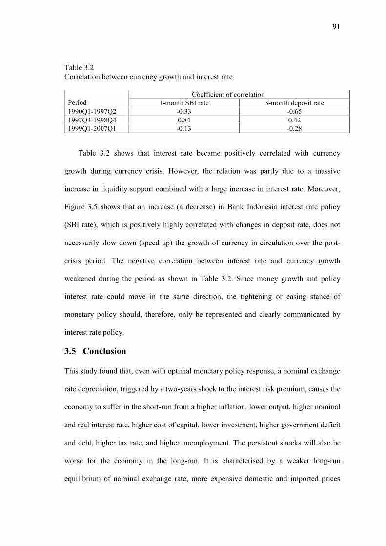
91
Table 3.2
Correlation between currency growth and interest rate
Period
Coefficient of correlation
1-month SBI rate 3-month deposit rate
1990Q1-1997Q2 -0.33 -0.65
1997Q3-1998Q4 0.84 0.42
1999Q1-2007Q1 -0.13 -0.28
Table 3.2 shows that interest rate became positively correlated with currency
growth during currency crisis. However, the relation was partly due to a massive
increase in liquidity support combined with a large increase in interest rate. Moreover,
Figure 3.5 shows that an increase (a decrease) in Bank Indonesia interest rate policy
(SBI rate), which is positively highly correlated with changes in deposit rate, does not
necessarily slow down (speed up) the growth of currency in circulation over the post-
crisis period. The negative correlation between interest rate and currency growth
weakened during the period as shown in Table 3.2. Since money growth and policy
interest rate could move in the same direction, the tightening or easing stance of
monetary policy should, therefore, only be represented and clearly communicated by
interest rate policy.
3.5 Conclusion
This study found that, even with optimal monetary policy response, a nominal exchange
rate depreciation, triggered by a two-years shock to the interest risk premium, causes the
economy to suffer in the short-run from a higher inflation, lower output, higher nominal
and real interest rate, higher cost of capital, lower investment, higher government deficit
and debt, higher tax rate, and higher unemployment. The persistent shocks will also be
worse for the economy in the long-run. It is characterised by a weaker long-run
equilibrium of nominal exchange rate, more expensive domestic and imported prices
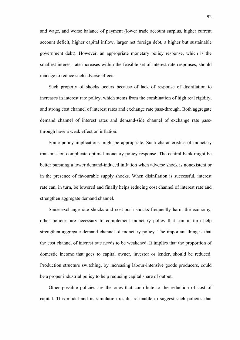
92
and wage, and worse balance of payment (lower trade account surplus, higher current
account deficit, higher capital inflow, larger net foreign debt, a higher but sustainable
government debt). However, an appropriate monetary policy response, which is the
smallest interest rate increases within the feasible set of interest rate responses, should
manage to reduce such adverse effects.
Such property of shocks occurs because of lack of response of disinflation to
increases in interest rate policy, which stems from the combination of high real rigidity,
and strong cost channel of interest rates and exchange rate pass-through. Both aggregate
demand channel of interest rates and demand-side channel of exchange rate pass-
through have a weak effect on inflation.
Some policy implications might be appropriate. Such characteristics of monetary
transmission complicate optimal monetary policy response. The central bank might be
better pursuing a lower demand-induced inflation when adverse shock is nonexistent or
in the presence of favourable supply shocks. When disinflation is successful, interest
rate can, in turn, be lowered and finally helps reducing cost channel of interest rate and
strengthen aggregate demand channel.
Since exchange rate shocks and cost-push shocks frequently harm the economy,
other policies are necessary to complement monetary policy that can in turn help
strengthen aggregate demand channel of monetary policy. The important thing is that
the cost channel of interest rate needs to be weakened. It implies that the proportion of
domestic income that goes to capital owner, investor or lender, should be reduced.
Production structure switching, by increasing labour-intensive goods producers, could
be a proper industrial policy to help reducing capital share of output.
Other possible policies are the ones that contribute to the reduction of cost of
capital. This model and its simulation result are unable to suggest such policies that
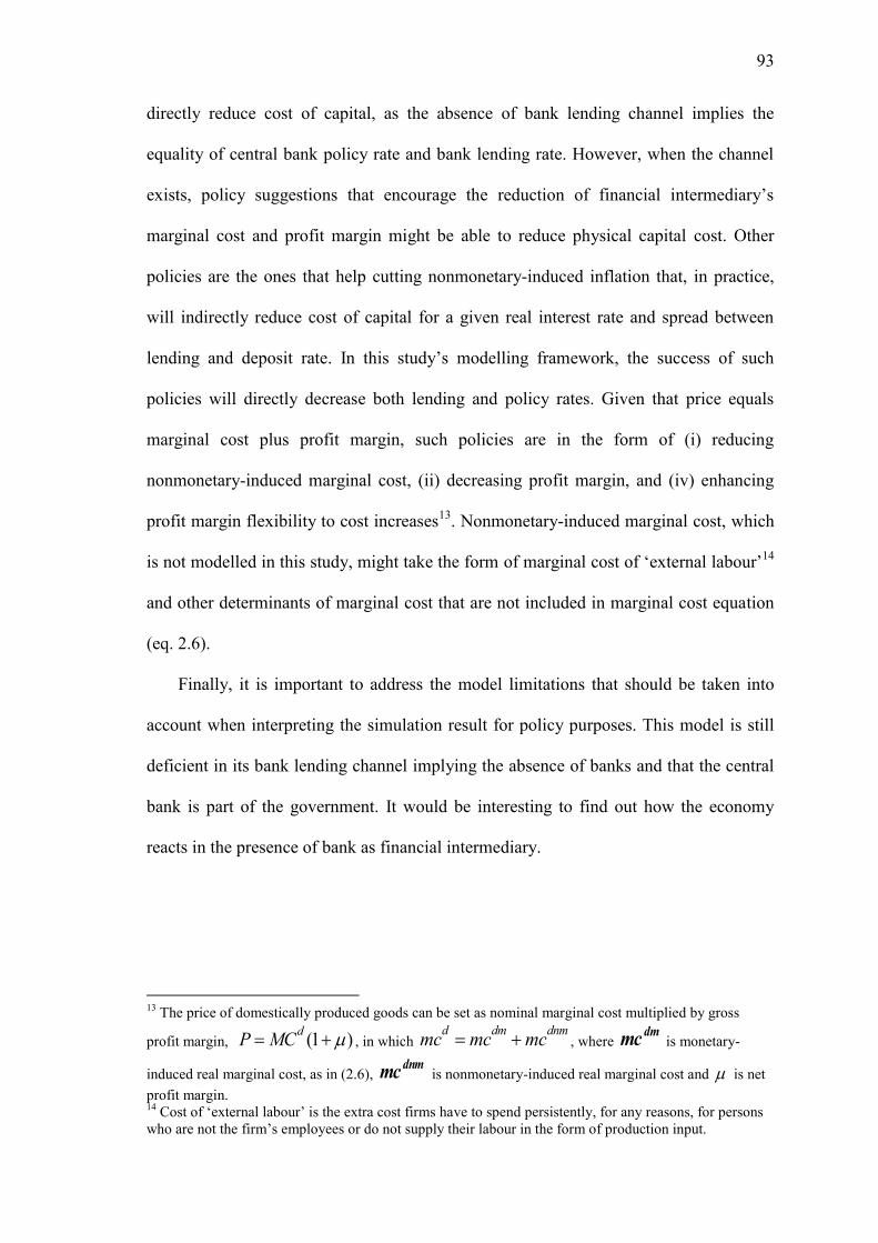
93
directly reduce cost of capital, as the absence of bank lending channel implies the
equality of central bank policy rate and bank lending rate. However, when the channel
exists, policy suggestions that encourage the reduction of financial intermediary‘s
marginal cost and profit margin might be able to reduce physical capital cost. Other
policies are the ones that help cutting nonmonetary-induced inflation that, in practice,
will indirectly reduce cost of capital for a given real interest rate and spread between
lending and deposit rate. In this study‘s modelling framework, the success of such
policies will directly decrease both lending and policy rates. Given that price equals
marginal cost plus profit margin, such policies are in the form of (i) reducing
nonmonetary-induced marginal cost, (ii) decreasing profit margin, and (iv) enhancing
profit margin flexibility to cost increases13
. Nonmonetary-induced marginal cost, which
is not modelled in this study, might take the form of marginal cost of ‗external labour‘14
and other determinants of marginal cost that are not included in marginal cost equation
(eq. 2.6).
Finally, it is important to address the model limitations that should be taken into
account when interpreting the simulation result for policy purposes. This model is still
deficient in its bank lending channel implying the absence of banks and that the central
bank is part of the government. It would be interesting to find out how the economy
reacts in the presence of bank as financial intermediary.
13
The price of domestically produced goods can be set as nominal marginal cost multiplied by gross
profit margin, )1( d
MCP , in which dnmdmd
mcmcmc , where dm
mc is monetary-
induced real marginal cost, as in (2.6), dnm
mc is nonmonetary-induced real marginal cost and is net
profit margin. 14
Cost of ‗external labour‘ is the extra cost firms have to spend persistently, for any reasons, for persons
who are not the firm‘s employees or do not supply their labour in the form of production input.
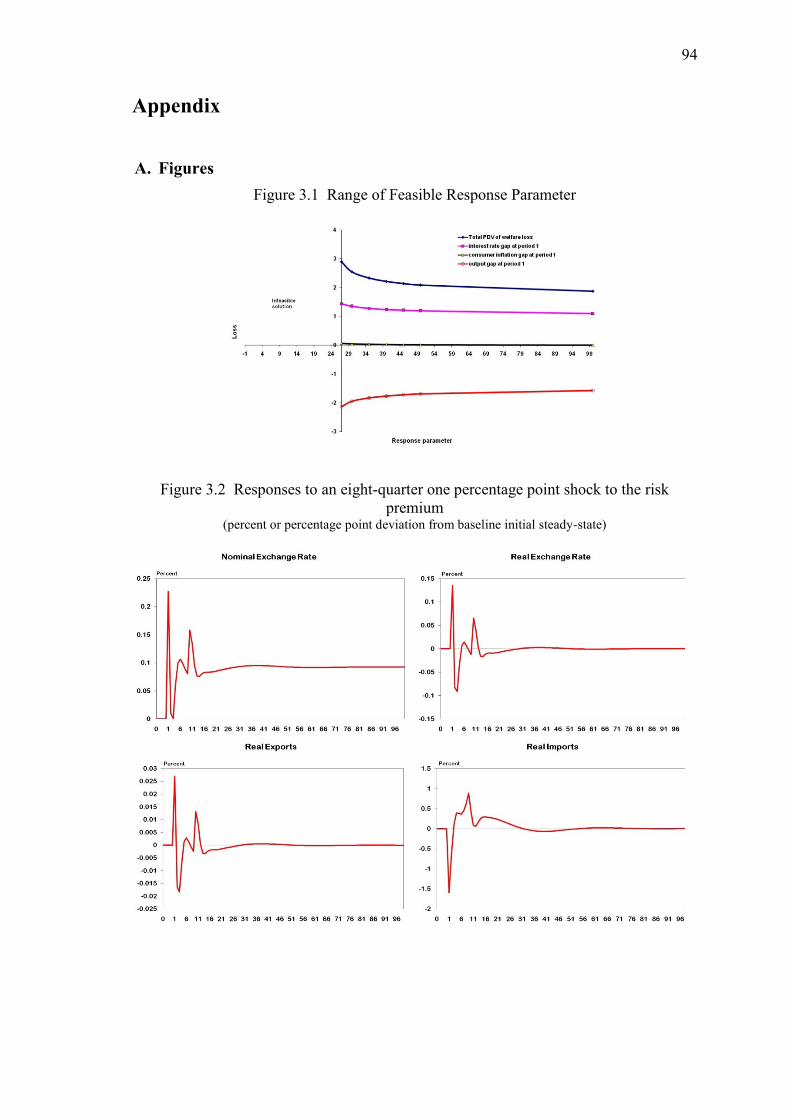
94
Appendix
A. Figures
Figure 3.1 Range of Feasible Response Parameter
Figure 3.2 Responses to an eight-quarter one percentage point shock to the risk
premium (percent or percentage point deviation from baseline initial steady-state)
95
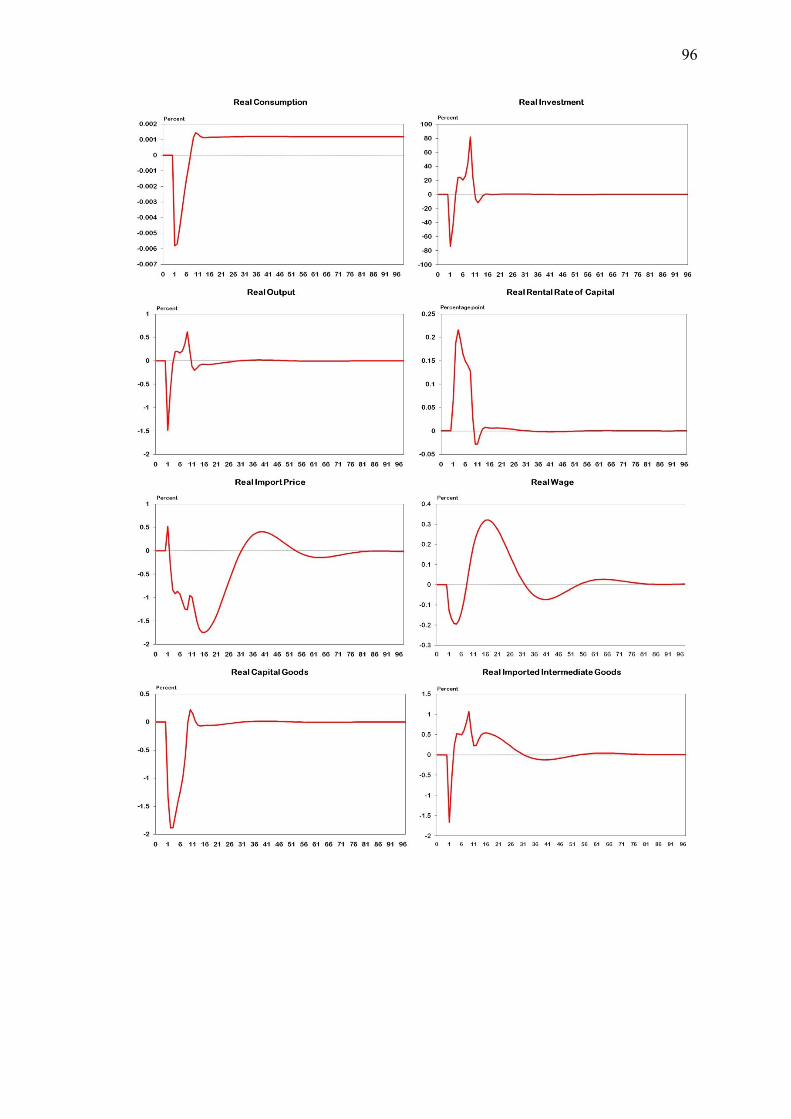
96
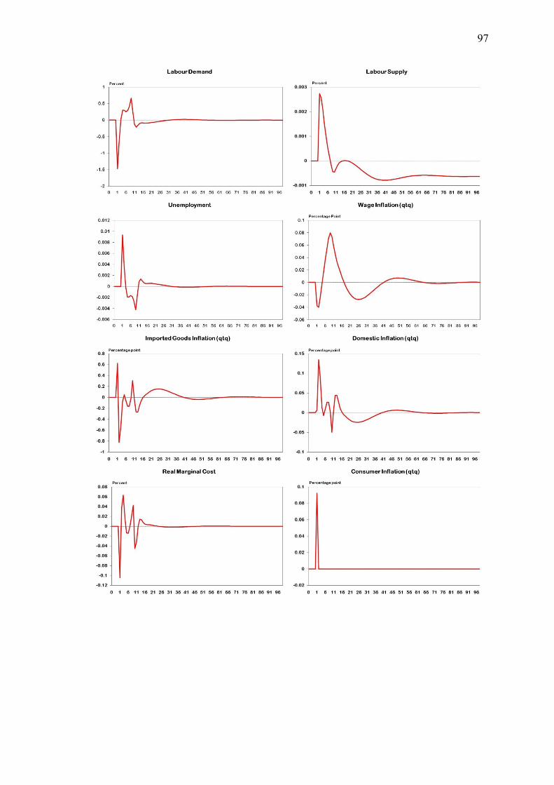
97
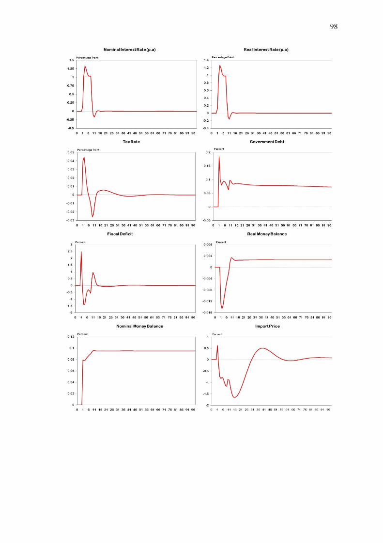
98
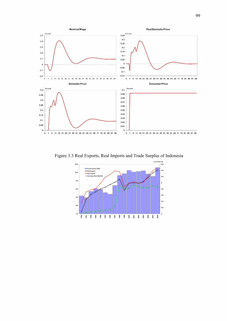
99
Figure 3.3 Real Exports, Real Imports and Trade Surplus of Indonesia
7.5
8.0
8.5
9.0
9.5
10.0
10.5
1990
1991
1992
1993
1994
1995
1996
1997
1998
1999
2000
2001
2002
2003
2004
2005
2006
5
5.2
5.4
5.6
5.8
6
6.2
6.4
6.6
Trade Surplus (US$)
Real Exports
Real Imports
Exchange Rate (Rp/US$)
log of billion Rp
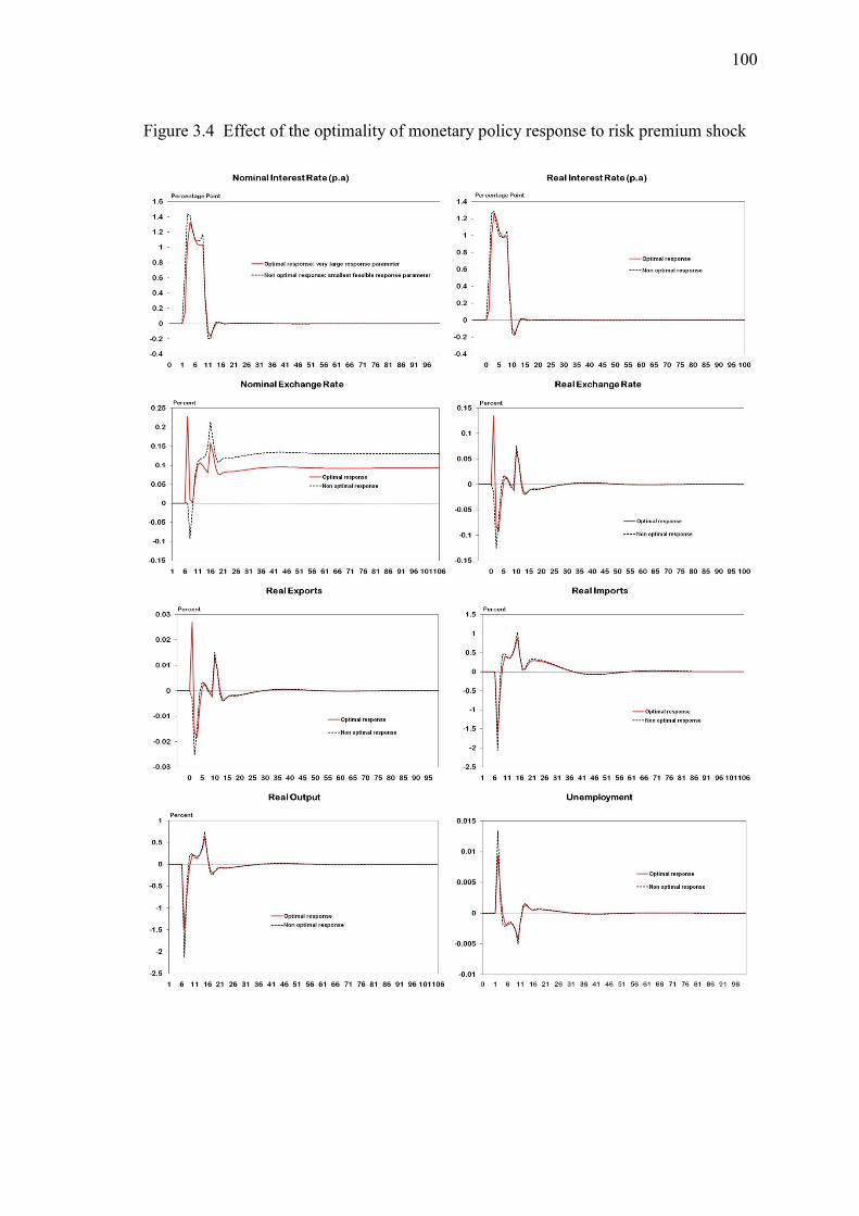
100
Figure 3.4 Effect of the optimality of monetary policy response to risk premium shock
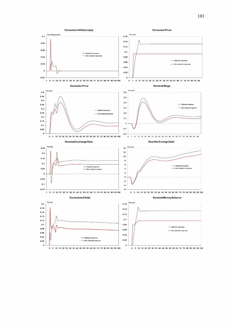
101
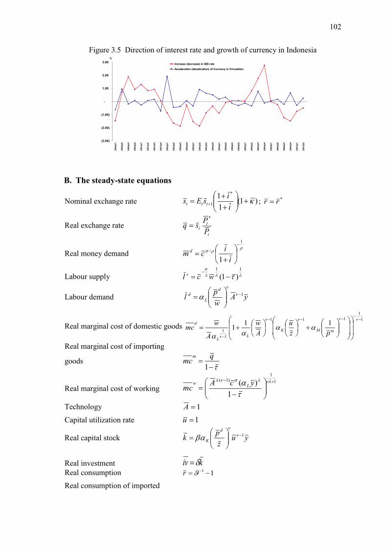
102
Figure 3.5 Direction of interest rate and growth of currency in Indonesia
B. The steady-state equations
Nominal exchange rate )1(1
1 *
1
i
isEs ttt ; *rr
Real exchange rate t
tt
P
Psq
*
Real money demand
1
/
1
i
icm d
Labour supply
11
)1(
wcl s
Labour demand yAw
pl
d
L
d 1
Real marginal cost of domestic goods 1
1
111
1
1
111
mMK
LL
d
pz
u
A
w
A
wmc
Real marginal cost of importing
goods
1
qmc
m
Real marginal cost of working 1
1)1(
1
)(
ycAmc L
w
Technology 1A
Capital utilization rate 1u
Real capital stock yuz
pk
d
K
1
Real investment kiv
Real consumption 11 r
Real consumption of imported
(3.00)
(2.00)
(1.00)
-
1.00
2.00
3.00
2000q
01
2000q
02
2000q
03
2000q
04
2001q
01
2001q
02
2001q
03
2001q
04
2002q
01
2002q
02
2002q
03
2002q
04
2003q
01
2003q
02
2003q
03
2003q
04
2004q
01
2004q
02
2004q
03
2004q
04
2005q
01
2005q
02
2005q
03
2005q
04
2006q
01
2006q
02
2006q
03
2006q
04
2007q
01
2007q
02
Increase (decrease) in SBI rate
Acceleration (deceleration) of Currency in Circulation
%
103
finished goods cc mcg
mcg
Real government consumption ygg r
Real exports ** yqx M
Real imports kgcgrm
imimimim
Real imports of raw material yp
pim
m
d
M
rm
Real imports of consumption goods ccim mcg
mcgcg
Real imports of capital goods ivim mkg
kg
Real demand for goods imxivgcy
Real output
1111111
)()()(
rm
tMK
d
L imkulAy
Consumer goods inflation mcgmcg md )1()1(1
)1(
Domestic goods inflation d
t
d
td MCMC 1loglog
Imported goods inflation m
t
m
tm MCMC 1loglog
Wage inflation w
t
w
tw MCMC 1loglog
Domestic goods‘ marginal cost d
t
d
t mcPMC
Imported goods‘ marginal cost m
t
m
t mcPMC
Nominal marginal cost of working w
t
w
t mcPCM
Consumer price )1(1 tt PP
Domestic goods price )1(1
d
t
d
t
d
t PP
Import price )1(1
mm
t
m
t PP
Nominal wage )1(1
w
tt WW
Real price of domestical good t
d
td
P
Pp
Real import price
1
qpm
Flexible real import price n
nmn q
p
1
Real wage 1
1)1(
1
)(
ycAw L
Real Rental price of capital
1
rz
Fiscal policy rule y
g
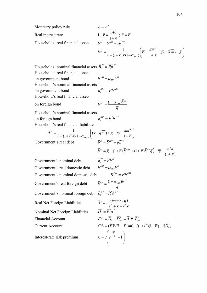
104
Monetary policy rule T
Real interest rate
1
11
ir ; *rr
Households‘ real financial assets *HHGH bqbb
gimqx
my
rrb
d
HG
H )(1)1()1(
1
Households‘ nominal financial assets H
t
H
t bPB
Households‘ real financial assets
on government bond H
HG
HG bb
Household‘s nominal financial assets
on government bond HG
t
HG
t bPB
Household‘s real financial assets
on foreign bond q
bb
H
HGH )1(*
Household‘s nominal financial assets
on foreign bond *** H
t
H
t bPB
Household‘s real financial liabilities
1)(
)1()1(
1 d
HG
H mygimqx
rrd
Government‘s real debt *GGHG bqbb
)1(
)1()1( *
sGGHG m
yqbbrgb
Government‘s nominal debt G
t
G
t bPB
Government‘s real domestic debt G
GH
GH bb
Government‘s nominal domestic debt GH
t
GH
t bPB
Government‘s real foreign debt q
bb
G
GHG )1(*
Government‘s nominal foreign debt *** G
t
G
t bPB
Real Net Foreign Liabilities **
* )/(
rr
qximd
Nominal Net Foreign Liabilities *** dPD tt
Financial Account *
1
***
1
*
tttt PdDDFA
Current Account *
1
** ]1)1)(1[()/( ttttt DiimPsxPCA
Interest-rate risk premium
1
*
y
bq
e
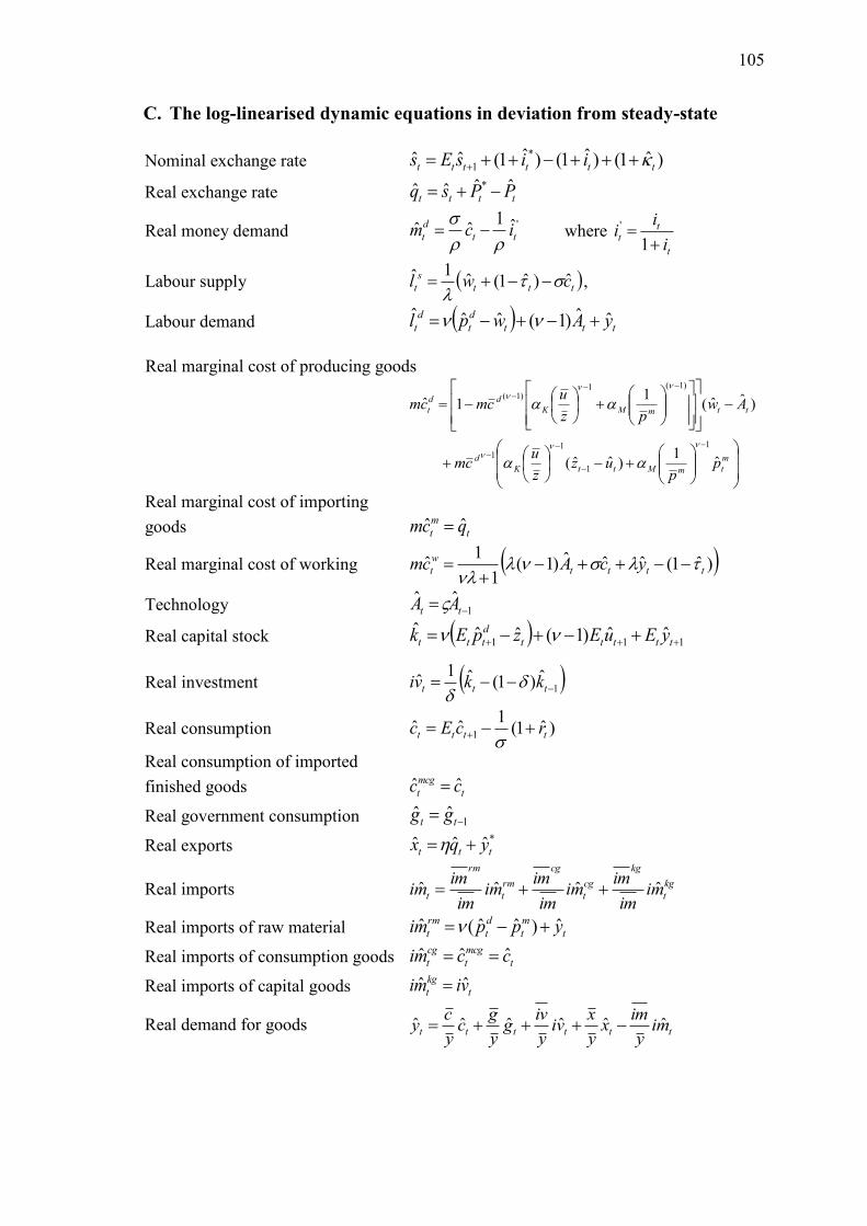
105
C. The log-linearised dynamic equations in deviation from steady-state
Nominal exchange rate )ˆ1()ˆ1()ˆ1(ˆˆ *
1 tttttt iisEs
Real exchange rate tttt PPsq ˆˆˆˆ *
Real money demand 'ˆ1
ˆˆtt
d
t icm
where
t
tt
i
ii
1
'
Labour supply ttt
s
t cwl ˆ)ˆ1(ˆ1ˆ
,
Labour demand ttt
d
t
d
t yAwpl ˆˆ)1(ˆˆˆ
Real marginal cost of producing goods
m
tmMttK
d
ttmMK
dd
t
pp
uzz
ucm
Awpz
ucmcm
ˆ1
)ˆˆ(
)ˆˆ(1
1ˆ
1
1
11
)1(1)1(
Real marginal cost of importing
goods t
m
t qcm ˆˆ
Real marginal cost of working )ˆ1(ˆˆˆ)1(1
1ˆ
tttt
w
t ycAcm
Technology 1ˆˆ tt AA
Real capital stock 111ˆˆ)1(ˆˆˆ ttttt
d
ttt yEuEzpEk
Real investment 1ˆ)1(ˆ1
ˆ ttt kkvi
Real consumption )ˆ1(1
ˆˆ1 tttt rcEc
Real consumption of imported
finished goods t
mcg
t cc ˆˆ
Real government consumption 1ˆˆ tt gg
Real exports *ˆˆˆttt yqx
Real imports kg
t
kg
cg
t
cg
rm
t
rm
t miim
immi
im
immi
im
immi ˆˆˆˆ
Real imports of raw material t
m
t
d
t
rm
t yppmi ˆ)ˆˆ(ˆ
Real imports of consumption goods t
mcg
t
cg
t ccmi ˆˆˆ
Real imports of capital goods t
kg
t vimi ˆˆ
Real demand for goods tttttt mi
y
imx
y
xvi
y
ivg
y
gc
y
cy ˆˆˆˆˆˆ
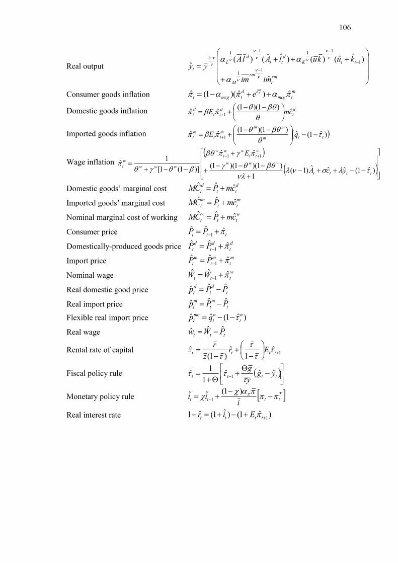
106
Real output
rm
t
rm
M
ttK
d
tt
d
L
t
miim
kukulAlAyy
ˆ
)ˆˆ()()ˆˆ()(ˆ
11
1
11111
Consumer goods inflation m
tmcg
d
tmcgt
ate ˆ)ˆ)(1(ˆ
ˆ
Domestic goods inflation d
t
d
tt
d
t cmE ˆ)1)(1(
ˆˆ1
Imported goods inflation )ˆ1(ˆ)1)(1(
ˆˆ1 ttm
mmm
tt
m
t qE
Wage inflation
)ˆ1(ˆˆˆ)1(1
)1)(1)(1(
ˆˆ
)]1(1[
1ˆ
11
tttt
www
w
tt
ww
t
w
www
w
t
ycA
E
Domestic goods‘ marginal cost d
tt
d
t cmPCM ˆˆˆ
Imported goods‘ marginal cost m
tt
m
t cmPCM ˆˆˆ
Nominal marginal cost of working w
tt
w
t cmPCM ˆˆˆ
Consumer price ttt PP ̂ˆˆ1
Domestically-produced goods price d
t
d
t
d
t PP ̂ˆˆ1
Import price m
t
m
t
m
t PP ̂ˆˆ1
Nominal wage w
ttt WW ̂ˆˆ1
Real domestic good price t
d
t
d
t PPp ˆˆˆ
Real import price t
m
t
m
t PPp ˆˆˆ
Flexible real import price )ˆ1(ˆˆ n
t
n
t
mn
t qp
Real wage ttt PWw ˆˆˆ
Rental rate of capital 1ˆ
1ˆ
)1(ˆ
tttt Er
z
rz
Fiscal policy rule
tttt yg
y
gˆˆˆ
1
1ˆ
1
Monetary policy rule T
tttti
ii
)1(ˆˆ1
Real interest rate )ˆ1()ˆ1(ˆ1 1 tttt Eir
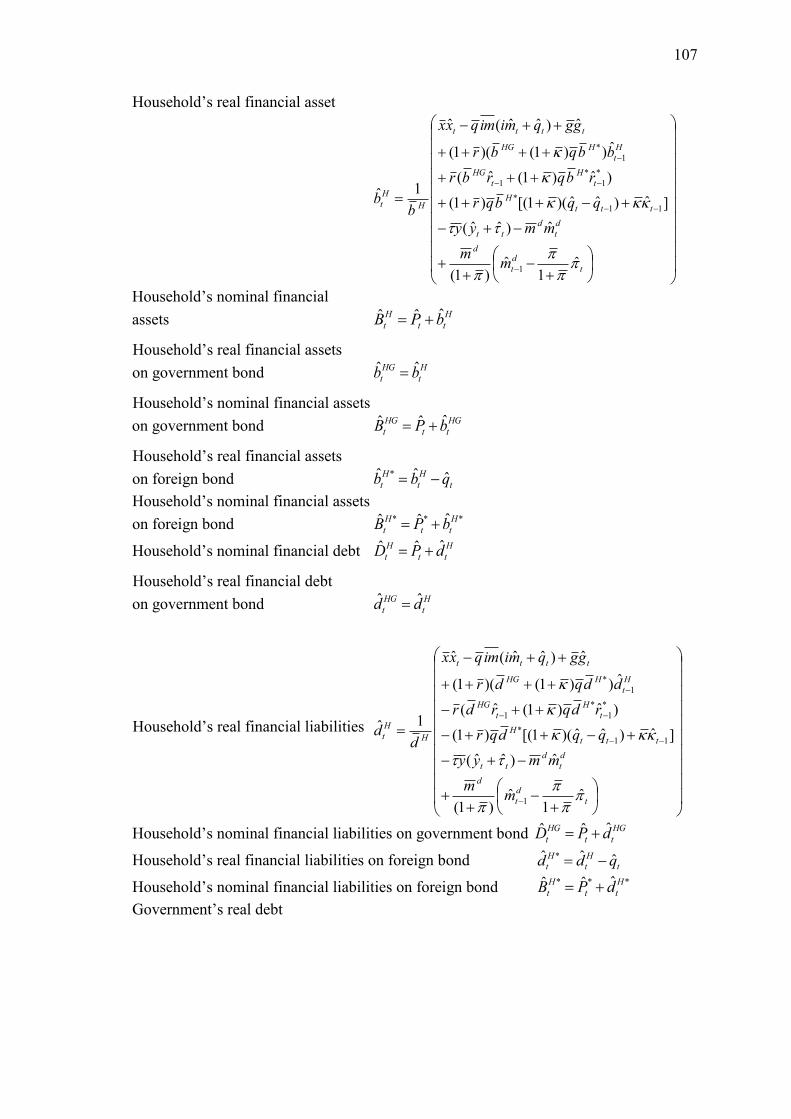
107
Household‘s real financial asset
t
d
t
d
d
t
d
tt
ttt
H
t
H
t
HG
H
t
HHG
tttt
H
H
t
mm
mmyy
qqbqr
rbqrbr
bbqbr
ggqmiimqxx
bb
ˆ1
ˆ)1(
ˆ)ˆˆ(
]ˆ)ˆˆ)(1[()1(
)ˆ)1(ˆ(
ˆ))1()(1(
ˆ)ˆˆ(ˆ
1ˆ
1
11
*
*
1
*
1
1
*
Household‘s nominal financial
assets H
tt
H
t bPB ˆˆˆ
Household‘s real financial assets
on government bond H
t
HG
t bb ˆˆ
Household‘s nominal financial assets
on government bond HG
tt
HG
t bPB ˆˆˆ
Household‘s real financial assets
on foreign bond t
H
t
H
t qbb ˆˆˆ *
Household‘s nominal financial assets
on foreign bond *** ˆˆˆ H
tt
H
t bPB
Household‘s nominal financial debt H
tt
H
t dPD ˆˆˆ
Household‘s real financial debt
on government bond H
t
HG
t dd ˆˆ
Household‘s real financial liabilities
t
d
t
d
d
t
d
tt
ttt
H
t
H
t
HG
H
t
HHG
tttt
H
H
t
mm
mmyy
qqdqr
rdqrdr
ddqdr
ggqmiimqxx
dd
ˆ1
ˆ)1(
ˆ)ˆˆ(
]ˆ)ˆˆ)(1[()1(
)ˆ)1(ˆ(
ˆ))1()(1(
ˆ)ˆˆ(ˆ
1ˆ
1
11
*
*
1
*
1
1
*
Household‘s nominal financial liabilities on government bond HG
tt
HG
t dPD ˆˆˆ
Household‘s real financial liabilities on foreign bond t
H
t
H
t qdd ˆˆˆ *
Household‘s nominal financial liabilities on foreign bond *** ˆˆˆ H
tt
H
t dPB
Government‘s real debt
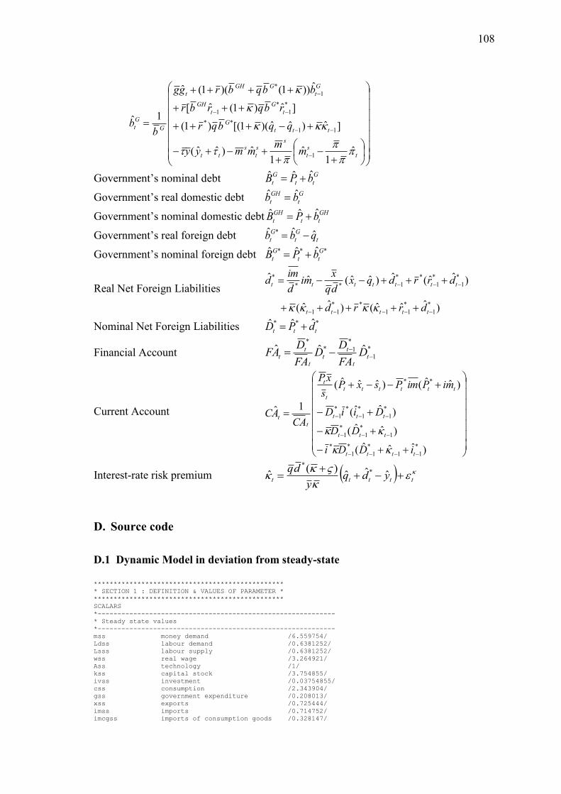
108
t
s
t
ss
t
s
tt
ttt
G
t
G
t
GH
G
t
GGH
t
G
G
t
mm
mmyy
qqbqr
rbqrbr
bbqbrgg
bb
ˆ1
ˆ1
ˆ)ˆˆ(
]ˆ)ˆˆ)(1[()1(
]ˆ)1(ˆ[
ˆ))1()(1(ˆ
1ˆ
1
11
**
*
1
*
1
1
*
Government‘s nominal debt G
tt
G
t bPB ˆˆˆ
Government‘s real domestic debt G
t
GH
t bb ˆˆ
Government‘s nominal domestic debt GH
tt
GH
t bPB ˆˆˆ
Government‘s real foreign debt t
G
t
G
t qbb ˆˆˆ *
Government‘s nominal foreign debt *** ˆˆˆ G
tt
G
t bPB
Real Net Foreign Liabilities
)ˆˆˆ()ˆˆ(
)ˆˆ(ˆ)ˆˆ(ˆˆ
*
1
*
11
**
11
*
1
*
1
**
1**
*
ttttt
ttttttt
drrd
drrdqxdq
xmi
d
imd
Nominal Net Foreign Liabilities *** ˆˆˆttt dPD
Financial Account *
1
*
1**
ˆˆˆ
tt
tt
t
tt D
FA
DD
FA
DAF
Current Account
)ˆˆˆ(
)ˆˆ(
)ˆˆ(
)ˆˆ()ˆˆˆ(
1ˆ
*
11
*
1
*
1
*
1
*
1
*
1
*
1
*
1
**
1
**
tttt
ttt
ttt
tttttt
t
t
tt
iDDi
DD
DiiD
miPimPsxPs
xP
CAAC
Interest-rate risk premium
ttttt ydq
y
dq
ˆˆˆ
)(ˆ *
*
D. Source code
D.1 Dynamic Model in deviation from steady-state
************************************************
* SECTION 1 : DEFINITION & VALUES OF PARAMETER *
************************************************
SCALARS
*------------------------------------------------------------
* Steady state values
*------------------------------------------------------------
mss money demand /6.559754/
Ldss labour demand /0.6381252/
Lsss labour supply /0.6381252/
wss real wage /3.264921/
Ass technology /1/
kss capital stock /3.754855/
ivss investment /0.03754855/
css consumption /2.343904/
gss government expenditure /0.208013/
xss exports /0.725444/
imss imports /0.714752/
imcgss imports of consumption goods /0.328147/
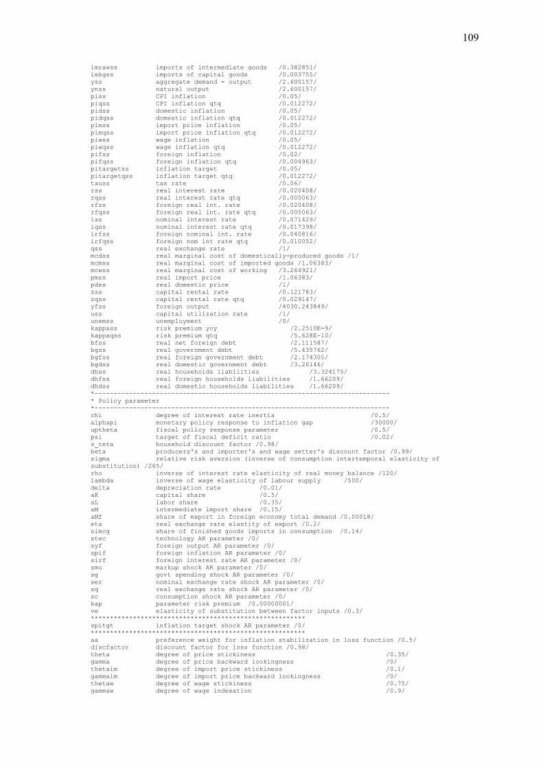
109
imrawss imports of intermediate goods /0.382851/
imkgss imports of capital goods /0.003755/
yss aggregate demand = output /2.600157/
ynss natural output /2.600157/
piss CPI inflation /0.05/
piqss CPI inflation qtq /0.012272/
pidss domestic inflation /0.05/
pidqss domestic inflation qtq /0.012272/
pimss import price inflation /0.05/
pimqss import price inflation qtq /0.012272/
piwss wage inflation /0.05/
piwqss wage inflation qtq /0.012272/
pifss foreign inflation /0.02/
pifqss foreign inflation qtq /0.004963/
pitargetss inflation target /0.05/
pitargetqss inflation target qtq /0.012272/
tauss tax rate /0.06/
rss real interest rate /0.020408/
rqss real interest rate qtq /0.005063/
rfss foreign real int. rate /0.020408/
rfqss foreign real int. rate qtq /0.005063/
iss nominal interest rate /0.071429/
iqss nominal interest rate qtq /0.017398/
irfss foreign nominal int. rate /0.040816/
irfqss foreign nom int rate qtq /0.010052/
qss real exchange rate /1/
mcdss real marginal cost of domestically-produced goods /1/
mcmss real marginal cost of imported goods /1.06383/
mcwss real marginal cost of working /3.264921/
pmss real import price /1.06383/
pdss real domestic price /1/
zss capital rental rate /0.121783/
zqss capital rental rate qtq /0.029147/
yfss foreign output /4030.243849/
uss capital utilization rate /1/
unemss unemployment /0/
kappass risk premium yoy /2.2510E-9/
kappaqss risk premium qtq /5.628E-10/
bfss real net foreign debt /2.111587/
bgss real government debt /5.435762/
bgfss real foreign government debt /2.174305/
bgdss real domestic government debt /3.26146/
dhss real households liabilities /3.324175/
dhfss real foreign households liabilities /1.66209/
dhdss real domestic households liabilities /1.66209/
*-----------------------------------------------------------------------------
* Policy parameter
*-----------------------------------------------------------------------------
chi degree of interest rate inertia /0.5/
alphapi monetary policy response to inflation gap /30000/
uptheta fiscal policy response parameter /0.5/
psi target of fiscal deficit ratio /0.02/
s_teta household discount factor /0.98/
beta producers's and importer's and wage setter's discount factor /0.99/
sigma relative risk aversion (inverse of consumption intertemporal elasticity of
substitution) /265/
rho inverse of interest rate elasticity of real money balance /120/
lambda inverse of wage elasticity of labour supply /500/
delta depreciation rate /0.01/
aK capital share /0.5/
aL labor share /0.35/
aM intermediate import share /0.15/
aMf share of export in foreign economy total demand /0.00018/
eta real exchange rate elastity of export /0.2/
simcg share of finished goods imports in consumption /0.14/
stec technology AR parameter /0/
syf foreign output AR parameter /0/
spif foreign inflation AR parameter /0/
sirf foreign interest rate AR parameter /0/
smu markup shock AR parameter /0/
sg govt spending shock AR parameter /0/
ser nominal exchange rate shock AR parameter /0/
sq real exchange rate shock AR parameter /0/
sc consumption shock AR parameter /0/
kap parameter risk premium /0.00000001/
ve elasticity of substitution between factor inputs /0.3/
********************************************************
spitgt inflation target shock AR parameter /0/
********************************************************
aa preference weight for inflation stabilization in loss function /0.5/
discfactor discount factor for loss function /0.98/
theta degree of price stickiness /0.35/
gamma degree of price backward lookingness /0/
thetaim degree of import price stickiness /0.1/
gammaim degree of import price backward lookingness /0/
thetaw degree of wage stickiness /0.75/
gammaw degree of wage indexation /0.9/
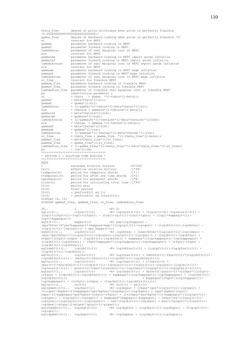
110
theta_flex degree of price stickiness when price is perfectly flexible
/0.00000000000000000000000000001/
gamma_flex degree of backward looking when price is perfectly flexible /0/
si constant for NKPC
gammab parameter backward looking in NKPC
gammaf parameter forward looking in NKPC
lambdakros parameter of real marginal cost in NKPC
sim constant for NKPC
gammaimb parameter backward looking in NKPC import goods inflation
gammaimf parameter forward looking in NKPC import goods inflation
lambdakrosim parameter of real marginal cost in NKPC import goods inflation
siw constant for NKPC
gammawb parameter backward looking in NKPC wage inflation
gammawf parameter forward looking in NKPC wage inflation
lambdakrosw parameter of real marginal cost in NKPC wage inflation
si_flex constant for flexible NKPC
gammab_flex parameter backward looking in flexible NKPC
gammaf_flex parameter forward looking in flexible NKPC
lambdakros_flex parameter of flexible real marginal cost in flesible NKPC
po substitution paremeter ;
si = theta + gamma *(1-theta*(1-beta));
gammaf = beta*theta*(1/si);
gammab = gamma*(1/si);
lambdakros = (1-gamma)*(1-theta)*(1-beta*theta)*(1/si);
sim = thetaim + gammaim*(1-thetaim*(1-beta));
gammaimf = beta*thetaim*(1/sim);
gammaimb = gammaim*(1/sim);
lambdakrosim = (1-gammaim)*(1-thetaim)*(1-beta*thetaim)*(1/sim);
siw = thetaw + gammaw *(1-thetaw*(1-beta));
gammawf = beta*thetaw*(1/siw);
gammawb = gammaw*(1/siw);
lambdakrosw = (1-gammaw)*(1-thetaw)*(1-beta*thetaw)*(1/siw);
si_flex = theta_flex + gamma_flex *(1-theta_flex*(1-beta));
gammaf_flex = beta*theta_flex*(1/si_flex);
gammab_flex = gamma_flex*(1/si_flex);
lambdakros_flex = (1-gamma_flex)*(1-theta_flex)*(1-beta*theta_flex)*(1/si_flex);
po = (ve-1)/ve;
*************************************
* SECTION 2 : SOLUTION TIME HORIZON *
*************************************
SETS
t extended solution horizon /0*100/
te(t) effective solution horizon /1*99/
ttemporer(t) period for temporary shocks /1*1/
ttemporer1(t) period for after one time shocks /2*2/
tpermanen(t) period for permanent shocks /1*8/
tloss(t) period for calculating total loss /1*99/
t0(t) period zero
tf(t) final period;
t0(t) = yes$(ord(t) eq 1);
tf(t) = yes$(ord(t) eq (card(t)));
DISPLAY t0, tf;
DISPLAY gammaf_flex, gammab_flex, si_flex, lambdakros_flex;
JD.. J =E= 0;
eq1(t+2).. log(er(t+1)) =E= log(erss(t+1)) + (log(er(t+2))-log(erss(t+2))) +
(log(1+irfq(t+1))-log(1+irfqss)) - (log(1+iq(t+1))-log(1+iqss)) + (log(1+kappaq(t+1))-
log(1+kappaqss));
eq1k(t+1).. kappa(t+1) =E= exp(log(kappass) +
(qss*bfss/(4*yss*kappass))*(kappass+kap)*((log(q(t+1))-log(qss)) + (log(bf(t+1))-log(bfss)) -
(log(y(t+1))-log(yss)))) + eps_kappa(t+1);
eq1bf(t+1).. log(bf(t+1)) =E= log(bfss) + (imss/bfss)*(log(im(t+1))-log(imss)) -
(xss/(qss*bfss))*((log(x(t+1))-log(xss))-(log(q(t+1))-log(qss))) + (log(bf(t))-log(bfss)) +
rfqss*((rfq(t)-rfqss) + (log(bf(t))-log(bfss))) + kappaqss*((log(kappaq(t))-log(kappaqss)) +
(log(bf(t))-log(bfss))) + rfqss*kappaqss*((log(kappaq(t))-log(kappaqss)) + (rfq(t)-rfqss) +
(log(bf(t))-log(bfss)));
eq1nombf(t+1).. log(nbf(t+1)) =E= log(nbfss(t+1)) + (log(pf(t+1))-log(pfss(t+1))) +
(log(bf(t+1))-log(bfss));
eq1fa(t+1).. log(fa(t+1)) =E= log(fass(t+1)) + (nbfss(t+1)/fass(t+1))*(log(nbf(t+1))-
log(nbfss(t+1))) - (nbfss(t)/fass(t+1))*(log(nbf(t))-log(nbfss(t)));
eq1ta(t+1).. log(ta(t+1)) =E= log(tass(t+1)) + 1/tass(t+1) *
(pss(t+1)*xss/erss(t+1)*((log(p(t+1))-log(pss(t+1)))+(log(x(t+1))-log(xss))-(log(er(t+1))-
log(erss(t+1)))) - pfss(t+1)*imss*((log(im(t+1))-log(imss))+(log(pf(t+1))-log(pfss(t+1)))));
eq1sa(t+1).. log(sa(t+1)) =E= log(sass(t+1)) + nbfss(t)/sass(t+1)*(irfqss*((irfq(t)-
irfqss) + (log(nbf(t))-log(nbfss(t)))) + kappaqss*((log(kappaq(t))-log(kappaqss)) + (log(nbf(t))-
log(nbfss(t)))) + kappaqss*irfqss*((log(kappaq(t))-
log(kappaqss)) + (irfq(t)-irfqss) + (log(nbf(t))-log(nbfss(t)))));
eq1ca(t+1).. ca(t+1) =E= ta(t+1) - sa(t+1);
eq1rgdebt(t+1).. log(bg(t+1)) =E= log(bgss) + 1/bgss*(gss*(log(g(t+1))-log(gss)) +
(1+rqss)*(bgdss+(1+kappaqss)*qss*bgfss)*(log(bg(t))-log(bgss)) + rqss*(bgdss*(rq(t)-
rqss)+(1+kappaqss)*qss*bgfss*(rfq(t)-rfqss)) + (1+rfqss)*qss*bgfss*((1+kappaqss)*((log(q(t+1))-
log(qss)) - (log(q(t))-log(qss))) + kappaqss*(kappaq(t)-kappaqss)) - tauss*yss*((log(y(t+1))-
log(yss))+(log(tau(t+1))-log(tauss))) - mss*(log(m(t+1))-log(mss)) + mss/(1+piqss)*((log(m(t))-
log(mss))-piqss/(1+piqss)*(piq(t+1)-piqss)));
eq1rfgdebt(t+1).. log(bgf(t+1)) =E= log(bgfss) + (log(bg(t+1))-log(bgss)) - (log(q(t+1))-
log(qss));
eq1rdgdebt(t+1).. log(bgd(t+1)) =E= log(bgdss) + (log(bg(t+1))-log(bgss));
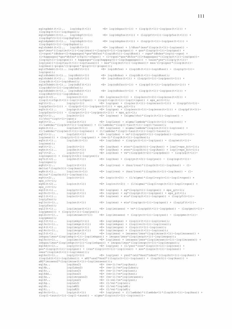
111
eq1ngdebt(t+1).. log(nbg(t+1)) =E= log(nbgss(t+1)) + (log(p(t+1))-log(pss(t+1))) +
(log(bg(t+1))-log(bgss));
eq1nfgdebt(t+1).. log(nbgf(t+1)) =E= log(nbgfss(t+1)) + (log(pf(t+1))-log(pfss(t+1))) +
(log(bgf(t+1))-log(bgfss));
eq1ndgdebt(t+1).. log(nbgd(t+1)) =E= log(nbgdss(t+1)) + (log(p(t+1))-log(pss(t+1))) +
(log(bgd(t+1))-log(bgdss));
eq1rhdebt(t+1).. log(dh(t+1)) =E= log(dhss) + 1/dhss*(xss*(log(x(t+1))-log(xss)) -
qss*imss*((log(im(t+1))-log(imss))+(log(q(t+1))-log(qss))) + gss*(log(g(t+1))-log(gss)) +
(1+rqss)*(dhdss+(1+kappaqss)*qss*dhfss)*(log(dh(t))-log(dhss)) - rqss*(dhdss*(rq(t)-rqss) +
(1+kappaqss)*qss*dhfss*(rfq(t)-rfqss)) - (1+rqss)*qss*dhfss*((1+kappaqss)*((log(q(t+1))-log(qss))-
(log(q(t))-log(qss))) + kappaqss*(log(kappaq(t))-log(kappaqss))) - tauss*yss*((log(y(t+1))-
log(yss))+(log(tau(t+1))-log(tauss))) - mss*(log(m(t+1))-log(mss))+ mss/(1+piqss)*((log(m(t))-
log(mss))-piqss/(1+piqss)*(piq(t+1)-piqss)));
eq1rfhdebt(t+1).. log(dhf(t+1)) =E= log(dhfss) + (log(dh(t+1))-log(dhss)) - (log(q(t+1))-
log(qss));
eq1rdhdebt(t+1).. log(dhd(t+1)) =E= log(dhdss) + (log(dh(t+1))-log(dhss));
eq1nhdebt(t+1).. log(ndh(t+1)) =E= log(ndhss(t+1)) + (log(p(t+1))-log(pss(t+1))) +
(log(dh(t+1))-log(dhss));
eq1nfhdebt(t+1).. log(ndhf(t+1)) =E= log(ndhfss(t+1)) + (log(pf(t+1))-log(pfss(t+1))) +
(log(dhf(t+1))-log(dhfss));
eq1ndhdebt(t+1).. log(ndhd(t+1)) =E= log(ndhdss(t+1)) + (log(p(t+1))-log(pss(t+1))) +
(log(dhd(t+1))-log(dhdss));
eq1n(t+2).. log(ern(t+1)) =E= log(erss(t+1)) + (log(ern(t+2))-log(erss(t+2))) +
(log(1+irfqn(t+1))-log(1+irfqss)) - (log(1+iqn(t+1))-log(1+iqss)) + eps_er(t+1);
eq2(t+1).. log(q(t+1)) =E= log(qss) + (log(er(t+1))-log(erss(t+1))) + (log(pf(t+1))-
log(pfss(t+1))) - (log(p(t+1))-log(pss(t+1))) + eps_q(t+1);
eq2n(t+1).. log(qn(t+1)) =E= log(qss) + (log(ern(t+1))-log(erss(t+1))) + (log(pf(t+1))-
log(pfss(t+1))) - (log(pn(t+1))-log(pss(t+1))) + eps_q(t+1);
eq3(t+1).. log(m(t+1)) =E= log(mss) + (sigma/rho)*(log(c(t+1))-log(css)) -
(1/rho)*(iq(t+1)-iqss);
eq4(t+1).. log(Ls(t+1)) =E= log(Lsss) - sigma/lambda*(log(c(t+1))-log(css)) +
(1/lambda)*(log(w(t+1))-log(wss)) + (1/lambda)*(log(1-tau(t+1))-log(1-tauss));
eq4n(t+1).. log(Lsn(t+1)) =E= log(Lsss) - sigma/lambda*(log(cn(t+1))-log(css)) +
(1/lambda)*(log(wn(t+1))-log(wss)) + (1/lambda)*(log(1-taun(t+1))-log(1-tauss));
eq5(t+1).. log(Ld(t+1)) =E= log(Ldss) + ve*((log(pd(t+1))-log(pdss))-(log(w(t+1))-
log(wss))) + (log(y(t+1))-log(yss)) + (ve-1)*(log(A(t+1))-log(Ass));
eq5n(t+1).. log(Ldn(t+1)) =E= log(Ldss) + (log(yn(t+1))-log(yss)) - (log(wn(t+1))-
log(wss));
eq6(t+1).. log(A(t+1)) =E= log(Ass) + stec*(log(A(t))-log(Ass)) + log(1+eps_A(t+1));
eq6n(t+1).. log(An(t+1)) =E= log(Ass) + stec*(log(A(t))-log(Ass)) + log(1+eps_A(t+1));
eq7(t+2).. log(k(t+1)) =E= log(kss) + ve*((log(pd(t+2))-log(pdss)) - (log(zq(t+1))-
log(zqss))) + (log(y(t+2))-log(yss));
eq7n(t+2).. log(kn(t+1)) =E= log(kss) + (log(yn(t+2))-log(yss)) - (log(zqn(t+1))-
log(zqss));
eq8(t+1).. log(iv(t+1)) =E= log(ivss) + (kss/ivss)*((log(k(t+1))-log(kss)) - (1-
delta)*(log(k(t))-log(kss)));
eq8n(t+1).. log(ivn(t+1)) =E= log(ivss) + (kss/ivss)*((log(kn(t+1))-log(kss)) - (1-
delta)*(log(kn(t))-log(kss)));
eq9(t+2).. log(c(t+1)) =E= log(c(t+2)) - (1/sigma)*(log(1+rq(t+1))-log(1+rqss)) +
eps_c(t+1);
eq9n(t+2).. log(cn(t+1)) =E= log(cn(t+2)) - (1/sigma)*(log(1+rqn(t+1))-log(1+rqss)) +
eps_c(t+1);
eq10(t+1).. log(g(t+1)) =E= log(gss) + sg*(log(g(t))-log(gss)) + eps_g(t+1);
eq10n(t+1).. log(gn(t+1)) =E= log(gss) + sg*(log(gn(t))-log(gss)) + eps_g(t+1);
eq11(t+1).. log(x(t+1)) =E= log(xss) + eta*(log(q(t+1))-log(qss)) + (log(yf(t+1))-
log(yfss));
eq11n(t+1).. log(xn(t+1)) =E= log(xss) + eta*(log(qn(t+1))-log(qss)) + (log(yf(t+1))-
log(yfss));
eq12(t+1).. log(imraw(t+1)) =E= log(imrawss) + ve*((log(pd(t+1))-log(pdss)) - (log(pm(t+1))-
log(pmss))) + (log(y(t+1))-log(yss));
eq12n(t+1).. log(imrawn(t+1)) =E= log(imrawss) + (log(yn(t+1))-log(yss)) - (log(pmn(t+1))-
log(pmss));
eq13(t+1).. log(imkg(t+1)) =E= log(imkgss) + (log(iv(t+1))-log(ivss));
eq13n(t+1).. log(imkgn(t+1)) =E= log(imkgss) + (log(ivn(t+1))-log(ivss));
eq14(t+1).. log(imcg(t+1)) =E= log(imcgss) + (log(c(t+1))-log(css));
eq14n(t+1).. log(imcgn(t+1)) =E= log(imcgss) + (log(cn(t+1))-log(css));
eq15(t+1).. log(im(t+1)) =E= log(imss) + imrawss/imss*(log(imraw(t+1))-log(imrawss)) +
imkgss/imss*(log(imkg(t+1))-log(imkgss)) + imcgss/imss*(log(imcg(t+1))-log(imcgss));
eq15n(t+1).. log(imn(t+1)) =E= log(imss) + imrawss/imss*(log(imrawn(t+1))-log(imrawss)) +
imkgss/imss*(log(imkgn(t+1))-log(imkgss)) + imcgss/imss*(log(imcgn(t+1))-log(imcgss));
eq16d(t+1).. log(y(t+1)) =E= log(yss) + (1/yss)*(css*(log(c(t+1))-log(css)) +
gss*(log(g(t+1))-log(gss)) + ivss*(log(iv(t+1))-log(ivss)) + xss*(log(x(t+1))-log(xss)) -
imss*(log(im(t+1))-log(imss)));
eq16s(t+1).. log(y(t+1)) =E= log(yss) + yss2*(aL2*Ass2*Ldss2*((log(A(t+1))-log(Ass)) +
(log(Ld(t+1))-log(Ldss))) + aK2*uss2*kss2*((log(u(t+1))-log(uss)) + (log(k(t))-log(kss))) +
aM2*imrawss2*(log(imraw(t+1))-log(imrawss)));
eq16a.. log(Ass2) =E= (ve-1)/ve*log(Ass);
eq16b.. log(Ldss2) =E= (ve-1)/ve*log(Ldss);
eq16c.. log(uss2) =E= (ve-1)/ve*log(uss);
eq16dd.. log(kss2) =E= (ve-1)/ve*log(kss);
eq16e.. log(imrawss2) =E= (ve-1)/ve*log(imrawss);
eq16f.. log(yss2) =E= (1-ve)/ve*log(yss);
eq16g.. log(aL2) =E= (1/ve)*log(aL);
eq16h.. log(aM2) =E= (1/ve)*log(aM);
eq16i.. log(aK2) =E= (1/ve)*log(aK);
eq16n(t+1).. log(yn(t+1)) =E= log(ynss) + (1/lambda)*((lambda+1)*(log(A(t+1))-log(Ass)) +
(log(1-taun(t+1))-log(1-tauss)) - sigma*(log(cn(t+1))-log(css)))-
112
lambda+1)/(aL*lambda)*(aK*(log(zqn(t+1))-log(zqss)) + aM*(log(pmn(t+1))-log(pmss)) - (log(pdn(t+1))-
log(pdss)));
eq17(t+1).. piq(t+1) =E= piqss + (1-simcg)*pidqss/piqss*((pidq(t+1)-
pidqss)+eps_adm(t+1)) + simcg*pimqss/piqss*(pimq(t+1)-pimqss) ;
eq17n(t+1).. piqn(t+1) =E= piqss + (1-simcg)*pidqss/piqss*(pidqn(t+1)-pidqss) +
simcg*pimqss/piqss*(pimqn(t+1)-pimqss) ;
eq18(t+1).. log(p(t+1)) =E= log(pss(t+1)) + (log(p(t))-log(pss(t))) + (piq(t+1)-piqss);
eq18n(t+1).. log(pn(t+1)) =E= log(pss(t+1)) + (log(pn(t))-log(pss(t))) + (piqn(t+1)-
piqss);
eq19(t+2).. pidq(t+1) =E= pidqss + gammab*(pidq(t)-pidqss) + gammaf*(pidq(t+2)-pidqss)
+ lambdakros*(log(mcd(t+1))-log(mcdss));
eq19n(t+1).. pidqn(t+1) =E= pidqss + (log(nmcdn(t+1)) - log(nmcdss(t+1))) -
(log(nmcdn(t)) - log(nmcdss(t)));
eq20(t+1).. log(npd(t+1)) =E= log(npdss(t+1)) + (log(npd(t))-log(npdss(t))) +
(log(1+pidq(t+1))-log(1+pidqss));
eq20n(t+1).. log(npdn(t+1)) =E= log(npdss(t+1)) + (log(npdn(t))-log(npdss(t))) +
(log(1+pidqn(t+1))-log(1+pidqss));
eq21(t+1).. log(pd(t+1)) =E= log(pdss) + (log(npd(t+1))-log(npdss(t+1))) - (log(p(t+1))-
log(pss(t+1)));
eq21n(t+1).. log(pdn(t+1)) =E= log(pdss) + (log(npdn(t+1))-log(npdss(t+1))) -
(log(pn(t+1))-log(pss(t+1)));
eq22(t+1).. log(mcd(t+1)) =E= log(mcdss) + (1-mcdss3*(aK*uss3/zqss3 +
aM/pmss3))*((log(w(t+1))-log(wss)) - (log(A(t+1))-log(Ass))) + mcdss3*uss3/zqss3*aK*((log(zq(t))-
log(zqss))) + mcdss3*1/pmss3*aM*(log(pm(t))-log(pmss)) + eps_mc(t+1);
eq22a.. log(mcdss3) =E= (ve-1)*log(mcdss);
eq22b.. log(uss3) =E= (ve-1)*log(uss);
eq22c.. log(zqss3) =E= (ve-1)*log(zqss);
eq22d.. log(pmss3) =E= (ve-1)*log(pmss);
eq22n(t+1).. log(mcdn(t+1)) =E= log(mcdss) + aL*(log(wn(t+1))-log(wss)) + aK*(log(zqn(t))-
log(zqss)) + aM*(log(pmn(t+1))-log(pmss)) - aL*(log(A(t+1))-log(Ass));
eq23(t+1).. log(nmcd(t+1)) =E= log(nmcdss(t+1)) + (log(mcd(t+1))-log(mcdss)) +
(log(p(t+1))-log(pss(t+1)));
eq23n(t+1).. log(nmcdn(t+1)) =E= log(nmcdss(t+1)) + (log(mcdn(t+1))-log(mcdss)) +
(log(pn(t+1))-log(pss(t+1)));
eq24(t+2).. pimq(t+1) =E= pimqss + gammaimb*(pimq(t)-pimqss) + gammaimf*(pimq(t+2)-
pimqss) + lambdakrosim*((log(q(t+1))-log(qss)) - (log(1-tau(t+1))-log(1-tauss)));
eq24n(t+1).. pimqn(t+1) =E= pimqss + (log(nmcmn(t+1)) - log(nmcmss(t+1))) -
(log(nmcmn(t)) - log(nmcmss(t)));
eq25(t+1).. log(npm(t+1)) =E= log(npmss(t+1)) + (log(npm(t))-log(npmss(t))) +
(log(1+pimq(t+1))-log(1+pimqss));
eq25n(t+1).. log(npmn(t+1)) =E= log(npmss(t+1)) + (log(npmn(t))-log(npmss(t))) +
(log(1+pimqn(t+1))-log(1+pimqss));
eq26(t+1).. log(pm(t+1)) =E= log(pmss) + (log(npm(t+1))-log(npmss(t+1))) - (log(p(t+1))-
log(pss(t+1)));
eq26n(t+1).. log(pmn(t+1)) =E= log(pmss) + (log(qn(t+1))-log(qss)) - (log(1-taun(t+1))-
log(1-tauss));
eq27(t+1).. log(mcm(t+1)) =E= log(mcmss) + (log(q(t+1))-log(qss)) - (log(1-tau(t+1))-
log(1-tauss));
eq27n(t+1).. log(mcmn(t+1)) =E= log(mcmss) + (log(qn(t+1))-log(qss));
eq28(t+1).. log(nmcm(t+1)) =E= log(nmcmss(t+1)) + (log(mcm(t+1))-log(mcmss)) +
(log(p(t+1))-log(pss(t+1)));
eq28n(t+1).. log(nmcmn(t+1)) =E= log(nmcmss(t+1)) + (log(mcmn(t+1))-log(mcmss)) +
(log(pn(t+1))-log(pss(t+1)));
eq29(t+2).. piwq(t+1) =E= piwqss + gammawb*(piwq(t)-piwqss) + gammawf*(piwq(t+2)-
piwqss) + lambdakrosw*1/(ve*lambda+1)*(lambda*(log(y(t+1))-log(yss)) + lambda*(ve-1)*(log(A(t+1))-
log(Ass)) + sigma*(log(c(t+1))-log(css)) - (log(1-tau(t+1))-log(1-tauss)));
eq29n(t+1).. piwqn(t+1) =E= piwqss + (log(nmcwn(t+1)) - log(nmcwss(t+1))) -
(log(nmcwn(t)) - log(nmcwss(t)));
eq30(t+1).. log(nw(t+1)) =E= log(nwss(t+1)) + (log(nw(t))-log(nwss(t))) +
(log(1+piwq(t+1))-log(1+piwqss));
eq31(t+1).. log(w(t+1)) =E= log(wss) + (log(nw(t+1))-log(nwss(t+1))) - (log(p(t+1))-
log(pss(t+1)));
eq31n(t+1).. log(wn(t+1)) =E= log(wss) + (1/(1+lambda))*(sigma*(log(cn(t+1))-log(css)) -
(log(1-taun(t+1))-log(1-tauss)) + lambda*(log(yn(t+1))-log(yss)));
eq32(t+1).. log(mcw(t+1)) =E= log(mcwss) + 1/(ve*lambda+1)*(lambda*(log(y(t+1))-log(yss))
+ lambda*(ve-1)*(log(A(t+1))-log(Ass)) + sigma*(log(c(t+1))-log(css)) + ve*lambda*(log(pd(t+1))-
log(pdss)) - (log(1-tau(t+1))-log(1-tauss)));
eq32n(t+1).. log(mcwn(t+1)) =E= log(mcwss) + (1/(1+lambda))*(sigma*(log(cn(t+1))-log(css)) -
(log(1-taun(t+1))-log(1-tauss)) + lambda*(log(yn(t+1))-log(yss)) );
eq33(t+1).. log(nmcw(t+1)) =E= log(nmcwss(t+1)) + (log(mcw(t+1))-log(mcwss)) +
(log(p(t+1))-log(pss(t+1)));
eq33n(t+1).. log(nmcwn(t+1)) =E= log(nmcwss(t+1)) + (log(mcwn(t+1))-log(mcwss)) +
(log(pn(t+1))-log(pss(t+1)));
eq34(t+1).. log(tau(t+1)) =E= log(tauss) + 1/(1+uptheta)*((log(tau(t))-log(tauss)) +
uptheta*gss/(tauss*yss)*((log(g(t+1))-log(gss))-(log(y(t+1))-log(yss))));
eq34n(t+1).. log(taun(t+1)) =E= log(tauss) + 1/(1+uptheta)*((log(taun(t))-log(tauss)) +
uptheta*gss/(tauss*yss)*((log(g(t+1))-log(gss))-(log(yn(t+1))-log(yss))));
eq35(t+2).. iq(t+1) =E= iqss + chi*(iq(t)-iqss) + ((1-
chi)/iqss)*alphapi*piqss*(piq(t+1)-pitargetq(t+1)) + eps_iq(t+1);
eq35n(t+2).. log(iqn(t+1)) =E= log(iqss) + chi*(log(iqn(t))-log(iqss)) + ((1-
chi)/iqss)*(alphapi1*(piqss*(piqn(t+2)-piqss) - pitargetqss*(pitargetqn(t+2)-pitargetqss)));
eq36(t+2).. log(1+rq(t+1)) =E= log(1+rqss) + (log(1+iq(t+1))-log(1+iqss)) -
(log(1+piq(t+2))-log(1+piqss));
eq36n(t+2).. log(1+rqn(t+1)) =E= log(1+rqss) + (log(1+iqn(t+1))-log(1+iqss)) -
(log(1+piqn(t+2))-log(1+piqss));
eq36f(t+2).. log(1+rfq(t+1)) =E= log(1+rfqss) + (log(1+irfq(t+1))-log(1+irfqss)) -
(log(1+pifq(t+2))-log(1+pifqss));
113
eq36fn(t+2).. log(1+rfqn(t+1)) =E= log(1+rfqss) + (log(1+irfqn(t+1))-log(1+irfqss)) -
(log(1+pifqn(t+2))-log(1+pifqss));
eq37(t+2).. zq(t+1) =E= zqss + 1/(zqss*(1-tauss))*iqss*(iq(t+1)-iqss) + tauss/(1-
tauss)*(log(tau(t+2))-log(tauss));
eq37n(t+1).. log(zqn(t+1)) =E= log(zqss) + 1/(zqss*(1-tauss))*(rqss*(log(rqn(t+1))-
log(rqss)) + (rqss+delta)/(1-tauss)*tauss*(log(taun(t+1))-log(tauss)));
eq38(t+1).. log(1+irfq(t+1)) =E= log(1+irfqss) + sirf*(log(1+irfq(t))-log(1+irfqss)) +
eps_irf(t+1);
eq38n(t+1).. log(1+irfqn(t+1)) =E= log(1+irfqss) + sirf*(log(1+irfqn(t))-log(1+irfqss)) +
eps_irf(t+1);
eq39(t+1).. log(1+pifq(t+1)) =E= log(1+pifqss) + spif*(log(1+pifq(t))-log(1+pifqss)) +
eps_pif(t+1);
eq39n(t+1).. log(1+pifqn(t+1)) =E= log(1+pifqss) + spif*(log(1+pifqn(t))-log(1+pifqss)) +
eps_pif(t+1);
eq40(t+1).. log(pf(t+1)) =E= log(pfss(t+1)) + (log(pf(t))-log(pfss(t))) +
(log(1+pifq(t+1))-log(1+pifqss));
eq40n(t+1).. log(pfn(t+1)) =E= log(pfss(t+1)) + (log(pfn(t))-log(pfss(t))) +
(log(1+pifqn(t+1))-log(1+pifqss));
eq41(t+1).. log(yf(t+1)) =E= log(yfss) + syf*(log(yf(t))-log(yfss)) + eps_yf(t+1);
eq41n(t+1).. log(yfn(t+1)) =E= log(yfss) + syf*(log(yfn(t))-log(yfss)) + eps_yf(t+1);
eq43(t+1).. 1+pi(t+1) =E= power((1+piq(t+1)),4);
eq44(t+1).. 1+pid(t+1) =E= power((1+pidq(t+1)),4);
eq45(t+1).. 1+pim(t+1) =E= power((1+pimq(t+1)),4);
eq46(t+1).. 1+pif(t+1) =E= power((1+pifq(t+1)),4);
eq47(t+1).. 1+piw(t+1) =E= power((1+piwq(t+1)),4);
eq48(t+1).. 1+i(t+1) =E= power((1+iq(t+1)),4);
eq49(t+1).. 1+irf(t+1) =E= power((1+irfq(t+1)),4);
eq50(t+1).. 1+z(t+1) =E= power((1+zq(t+1)),4);
eq51(t+1).. 1+r(t+1) =E= power((1+rq(t+1)),4);
eq52(t+1).. pitargetq(t+1) =E= pitargetqss + eps_pitargetq(t+1);
eq53(t+1).. 1+kappaq(t+1) =E= sqrt(sqrt(1+kappa(t+1)));
eq54(t+1).. unem(t+1) =E= Ls(t+1) - Ld(t+1);
eq55(t+1).. bop(t+1) =E= ca(t+1) + fa(t+1);
eqloss.. losstotal =E= sum(tloss,
power(discfactor,ord(tloss))*(aa*(power((100*(piq.l(tloss)-pitargetq(tloss))),2)) + (1-
aa)*(power((100*(log(y.l(tloss))-log(yss))),2))));
D.2 Steady-State Model
********************************
* SECTION 1 : PARAMETER VALUES *
********************************
SCALARS
s_teta household discount factor /0.98/
beta producers's and importer's and wage setter's discount factor /1/
sigma relative risk aversion (inverse of consumption intertemporal elasticity of
substitution) /125/
rho inverse of interest rate elasticity of real money balance /25/
lambda inverse of wage elasticity of labour supply /50/
delta depreciation rate /0.01/
aK capital share /0.35/
aL labor share /0.50/
aM intermediate import share /0.15/
aMf share of export in foreign economy total demand /0.01/
eta price elastity of export /0.5/
simkg share of imports in investment /0.14/
simcg share of finished goods imports in consumption /0.14/
gpy government expenditure-to-GDP ratio /0.08/
xpy exports-to-GDP ratio /0.30/
*-----------------------------------------------------------------------------
* Policy parameter
*-----------------------------------------------------------------------------
chi degree of interest rate inertia /0.5/
alphapi monetary policy response to inflation gap /1.5/
uptheta fiscal policy response parameter /0.5/
psi target of fiscal deficit ratio /0.02/
*-----------------------------------------------------------------------------
theta degree of price stickiness /0.5/
gamma degree of price backward lookingness /0.00/
thetaim degree of import price stickiness /0.3/
gammaim degree of import price backward lookingness /0.00/
thetaw degree of wage stickiness /0.75/
gammaw degree of wage indexation /0.00/
theta_flex degree of price stickiness when price is perfectly flexible /0.00000000000001/
gamma_flex degree of backward looking when price is perfectly flexible /0/
si constant for NKPC
gammab parameter backward looking in NKPC
gammaf parameter forward looking in NKPC
lambdakros parameter of real marginal cost in NKPC
sim constant for NKPC
gammaimb parameter backward looking in NKPC import goods inflation
gammaimf parameter forward looking in NKPC import goods inflation
lambdakrosim parameter of real marginal cost in NKPC import goods inflation
siw constant for NKPC
gammawb parameter backward looking in NKPC wage inflation
114
gammawf parameter forward looking in NKPC wage inflation
lambdakrosw parameter of real marginal cost in NKPC wage inflation
si_flex constant for flexible NKPC
gammab_flex parameter backward looking in flexible NKPC
gammaf_flex parameter forward looking in flexible NKPC
lambdakros_flex parameter of flexible real marginal cost in flesible NKPC ;
si = theta + gamma *(1-theta*(1-beta));
gammaf = beta*theta*(1/si);
gammab = gamma*(1/si);
lambdakros = (1-gamma)*(1-theta)*(1-beta*theta)*(1/si);
sim = thetaim + gammaim*(1-thetaim*(1-beta));
gammaimf = beta*thetaim*(1/sim);
gammaimb = gammaim*(1/sim);
lambdakrosim = (1-gammaim)*(1-thetaim)*(1-beta*thetaim)*(1/sim);
siw = thetaw + gammaw *(1-thetaw*(1-beta));
gammawf = beta*thetaw*(1/siw);
gammawb = gammaw*(1/siw);
lambdakrosw = (1-gammaw)*(1-thetaw)*(1-beta*thetaw)*(1/siw);
si_flex = theta_flex + gamma_flex *(1-theta_flex*(1-beta));
gammaf_flex = beta*theta_flex*(1/si_flex);
gammab_flex = gamma_flex*(1/si_flex);
lambdakros_flex = (1-gamma_flex)*(1-theta_flex)*(1-beta*theta_flex)*(1/si_flex);
***************************************
* SECTION 3 : COMPUTATION OF SOLUTION *
***************************************
JD.. J =E= 0;
eq1(t).. log(erss(t)) =E= log(er0) + ord(t)*(log(1+iqss(t))-log(1+irfqss(t)));
eq2(t).. log(qss(t)) =E= log(erss(t)) + log(pfss(t)) - log(pss(t));
eq3(t).. log(mss(t)) =E= (sigma/rho)*log(css(t)) - (1/rho)*iqss(t);
eq4(t).. log(Lsss(t)) =E= (-sigma/lambda)*log(css(t)) + (1/lambda)*log(wss(t)) +
(1/lambda)*log(1-tauss(t));
eq5(t).. log(Ldss(t)) =E= log(aL) + log(pdss(t)) + log(yss(t)) - log(wss(t));
eq9(t).. log(kss(t)) =E= log(beta) + log(aK) + log(pdss(t)) + log(yss(t)) -
log(zqss(t));
eq10(t).. log(ivss(t)) =E= log(delta) + log(kss(t));
eq11(t).. gss(t) =E= gpy*yss(t);
eq12(t).. log(xss(t)) =E= log(aMf) + eta*log(qss(t)) + log(yfss(t));
eq16(t).. imss(t) =E= imrawss(t) + imkgss(t) + imcgss(t);
eq13(t).. log(imrawss(t)) =E= log(aM) + log(pdss(t)) + log(yss(t)) - log(pmss(t));
eq14(t).. log(imkgss(t)) =E= log(simkg) + log(ivss(t));
eq15(t).. log(imcgss(t)) =E= log(simcg) + log(css(t));
eq17(t).. yss(t) =E= css(t)+gss(t)+ivss(t)+xss(t)-imss(t);
eq18(t).. log(yss(t)) =E= aL*log(Ass) + aL*log(Lsss(t)) + aK*log(uss(t)) + aK*log(kss(t))
+ aM*log(imrawss(t));
eq19(t).. log(yss(t)) =E= (1/lambda)*(log(1-tauss(t)) - sigma*log(css(t)) + log(aL))
+ ((lambda+1)/lambda)*(log(Ass) - (aK/aL)*log(zqss(t)) - (aM/aL)*log(qss(t))) + (1+lambda*(1-
aL))/(lambda*aL)*log(pdss(t)) + ((lambda+1)/(aL*lambda))*(aK*log(aK) + aM*log(aM));
eq21(t).. log(pss(t)) =E= log(p0) + ord(t)*log(1+piqss(t));
eq30(t).. piqss(t) =E= pitargetqss;
eq31(t).. piqss(t) =E= (1-simcg)*pidqss(t) + simcg*pimqss(t);
eq32(t).. log(npdss(t)) =E= log(p0) + ord(t)*log(1+pidqss(t));
eq33(t).. log(pdss(t)) =E= log(npdss(t)) - log(pss(t));
eq7(t).. log(mcdss(t)) =E= aL*log(wss(t))+aK*log(zqss(t))+aM*log(pmss(t))-aL*log(Ass)-
aL*log(aL)-aK*log(aK)-aM*log(aM);
eq8(t).. log(nmcdss(t)) =E= log(mcdss(t)) + log(pss(t));
eq22(t).. log(pmss(t)) =E= log(qss(t));
eq23(t).. npmss(t) =E= pmss(t)*pss(t);
eq24(t).. log(1+pimqss(t)) =E= (1/ord(t))*(log(npmss(t))-log(p0));
eq24a(t).. log(1+pimqss(t)) =E= (1/ord(t))*(log(nmcmss(t))-log(p0*mcmss('1')));
eq7m(t).. log(mcmss(t)) =E= log(qss(t));
eq8m(t).. log(nmcmss(t)) =E= log(mcmss(t)) + log(pss(t));
eq6(t).. log(wss(t)) =E= (1/(1+lambda))*(sigma*log(css(t)) - log(1-tauss(t)) +
lambda*log(pdss(t)) + lambda*log(yss(t)) + lambda*log(aL));
eq37(t).. nwss(t) =E= wss(t)*pss(t);
eq38(t).. log(1+piwqss(t)) =E= (1/ord(t))*(log(nwss(t))-log(p0*wss('1')));
eq38a(t).. log(1+piwqss(t)) =E= (1/ord(t))*(log(nmcwss(t))-log(p0*mcwss('1')));
eq7w(t).. log(mcwss(t)) =E= (1/(1+lambda))*(sigma*log(css(t)) - log(1-tauss(t)) +
lambda*log(pdss(t)) + lambda*log(yss(t)) + lambda*log(aL));
eq8w(t).. log(nmcwss(t)) =E= log(mcwss(t)) + log(pss(t));
eq25(t).. log(pfss(t)) =E= log(p0) + ord(t)*log(1+pifqss(t));
eq26(t).. 1+irfss(t) =E= (1+rfss(t))*(1+pifss(t));
eq27(t).. 1+iss(t) =E= (1+rss(t))*(1+piss(t));
eq28(t).. zss(t) =E= rss(t)+(power((1+delta),4)-1);
eq29(t).. tauss(t) =E= gss(t)/yss(t)-psi;
eq34(t).. rss(t) =E= 1/s_teta-1;
eq35(t).. rfss(t) =E= rss(t);
eq36(t).. log(yfss(t)) =E= log(xpy)+log(yss(t))-log(aMf)-eta*log(qss(t));
eq39(t).. uss(t) =E= 1;
eq40(t).. 1+piss(t) =E= power((1+piqss(t)),4);
eq41(t).. 1+pidss(t) =E= power((1+pidqss(t)),4);
eq42(t).. 1+pimss(t) =E= power((1+pimqss(t)),4);
eq43(t).. 1+pifqss(t) =E= sqrt(sqrt(1+pifss(t)));
eq44(t).. 1+piwss(t) =E= power((1+piwqss(t)),4);
eq45(t).. 1+iqss(t) =E= sqrt(sqrt(1+iss(t)));
eq46(t).. 1+irfqss(t) =E= sqrt(sqrt(1+irfss(t)));
eq47(t).. 1+zqss(t) =E= sqrt(sqrt(1+zss(t)));
eq48(t).. 1+rqss(t) =E= sqrt(sqrt(1+rss(t)));
eq49(t).. 1+rfqss(t) =E= sqrt(sqrt(1+rfss(t)));
Chapter 4
Indonesia’s inflation determinant: demand-pull vs. cost-push
116
4.1 Introduction
Previous study using a dynamic general equilibrium model in chapter 3 found the
existence of strong cost channel and weak demand channel of monetary transmission in
Indonesia‘s economy. Consequently, inflation is insensitive to monetary contraction, or
in other words, a higher interest rate is less effective in reducing inflation. The finding is
consistent with empirical study using macroeconometric model that estimated a low
sensitivity of inflation to interest rate changes (Majardi, 2004). One can also imply the
existence of strong cost channel of Bank Indonesia‘s interest rate policy to GDP deflator
from a price puzzle finding in a previous study on monetary transmission of Indonesia
(Agung, 2001). The aforementioned findings might bring about question whether
interest rate policy has a quite powerful control on Indonesia‘s inflation.
There are several modelling features that might be able to provide insights about
how monetary policy can have influential control on inflation. First, one needs to
distinguish between interest policy rate, which is a signalling rate, and market interest
rates that affect supply of and demand for goods and nonfinancial nonpublic services
(henceforth called services). Second, interest rate cost channel to inflation needs to be
separated into credit and equity interest cost channel. Third, interest rate cost channel
should be linked to an interest rate-driven demand channel and interest rate-based
measure of profit margin. Fourth, goods and services production needs to be linked with
variety sources of capital stock financing by elaborating physical capital stock into real
equity capital and real loan capital. Finally, it is essential to make a distinction in
inflation determinant between cost and demand–supply interaction.
Macroeconometric models usually put less emphasis on modelling goods
production cost as an inflation determinant. Current approaches mainly consider that
sources of inflation pressure are output gap, which is a discrepancy between actual
117
output and trend of output, inflation expectation and shocks to the supply of goods and
services.
Modelling goods production cost empirically as an inflation determinant usually
employs a partial equilibrium approach. In a mark-up model, which is applied for
instance by deBrouwer & Ericson (1998) and Bailliu, et al. (2002), general domestic
price level is a mark-up to total unit cost, which consist of unit labour cost, imported
raw material price and energy price.
A newer approach for modelling cost as inflation determinant is a new Keynesian
Phillips curve model, which is based on a study about staggered price setting behaviour
(Taylor, 1980 and Calvo, 1983) and usually built-in in a dynamic general equilibrium
model. In this model, firms‘ behaviour in setting their price optimally results in a
relationship between inflation and expected inflation and real marginal cost.
This study analyses inflation determinant using a macroeconomic general
equilibrium model with five representative agents (firm, bank, central bank, government
and household), each agent has own budget and balance sheet constraints, and objective
function. Model coefficients are calibrated with values that as closely as possible
represent the structure of Indonesia‘s economy. The steady-state model provides sets of
steady-state values of endogenous variables that describe economic structure, i.e.
breakdown of output, consumption, currency holding, labour supply and demand,
production structures and loans components.
This study aimed to gain an alternative analytical economic framework that can
offer a conceptual support for policy analysis and judgement in policy decision making.
It also serves as a preliminary research for further analysis involving dynamic
simulations of shocks to the economy, particularly to financial services.
118
The analysis shows that the strongest effect of interest rate increases to demand-
pull inflation works through investment demand and profit margin channel, which could
have a restraining effect on supply hence causing likelihood to have a higher, instead of
lower, inflation. Combined with a strong interest rate cost-push channel and market
power, this study enhances the previous analysis on why an interest rate tightening has a
weak control on reducing inflation in Indonesia.
The weak demand channel and strong cost channel of interest rates have some
implications for the behaviour of and policy for banking related to the achievement of
inflation target. First, the rate of interest on depositing funds at banks serves as a subset
of rate of return on equity capital in all profit-maximising business units that
subsequently affect firms‘ decision on price of goods and services. Thus, central bank‘s
ability to drive interbank rate appropriately is crucial since interbank rate is a main
determinant of deposit rate. Second, policy rate pass-through to lending rate also
depends on capital adequacy ratio, meaning that the ratio is impliedly an inflation
determinant. Therefore, banking policy is necessary to support the achievement of
monetary authority‘s target through setting an inflation-oriented optimal range of capital
adequacy ratio. Third, potential conflict between monetary and banking policy can be
weak or even nonexistent in a certain period, in the economy with such properties of
monetary transmission mechanism.
The rest of this paper is organized follows. Section 4.2 presents model development
to provide the aforementioned features. Section 4.3 provides analysis about demand-
pull and cost-push inflation. Section 4.4 explains the steady-state simulation results.
Section 4.5 concludes the study and infers some policy recommendations.
119
4.2 The model
This study extends dynamic general equilibrium model developed in chapter 3 by
adding the commercial bank and separating the central bank from the government. It
allows the presence of different interest rates in financial system and pass-through of
central bank signalling policy rate to market interest rates. This framework will enhance
the cost channel analysis and provide bank lending channel of monetary policy. The
model‘s extension is described as follows.
4.2.1 The firm
The monopolistically competitive firm maximizes its lifetime after-tax net return on
equities (ROE), max
0
~
t
p
t
t , subject to production function and balance sheet, where
0)1(~
11
ep
tt
i
t
p
t Kip
is defined as the difference between the firm‘s after-tax gross
ROE,
pt , and after-tax cost of equity,
ep
t
D
t
i
t Ki 1
~
1)1( . The latter denotes the household-
investor‘s opportunity cost of investing money on the business of producing goods and
services, instead of putting money on financial product (financial investment). This
principle makes sure that the firm‘s business profit will be greater than interest income
earned from placing fund on financial assets, ep
t
D
t
i
t
ep
t
D
t
i
t
p
t
p
t KiKi 1
~
11
~
1 )1()1(~
.
In steady-state firms operate in a perfectly competitive market, where net rate of ROE is
absent. In other words, ROE equals cost of equity capital in steady-state.
Similar with the idea in Christiano, et al. (2007), I assume that firms require the
stock of working capital loans and equities to finance part of intermediate inputs due to
production and sales throughput time as well as a need to keep a certain inventory level
of raw material or merchandise. Flow of loans, equity shares and accumulated retained
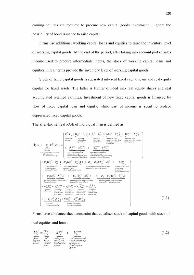
120
earning equities are required to procure new capital goods investment. I ignore the
possibility of bond issuance to raise capital.
Firms use additional working capital loans and equities to raise the inventory level
of working capital goods. At the end of the period, after taking into account part of sales
income used to procure intermediate inputs, the stock of working capital loans and
equities in real terms provide the inventory level of working capital goods.
Stock of fixed capital goods is separated into real fixed capital loans and real equity
capital for fixed assets. The latter is further divided into real equity shares and real
accumulated retained earnings. Investment of new fixed capital goods is financed by
flow of fixed capital loan and equity, while part of income is spent to replace
depreciated fixed capital goods.
The after-tax net real ROE of individual firm is defined as
equityonreturnrealgrossontaxincome
ep
tjtj
D
tj
i
t
equityofstcorealtaxafter
ep
tj
D
tj
i
t
stconterestiloancapital
fixedreal
fc
tj
L
t
ostcnterestiloancapital
workingreal
wc
tj
L
t
stcogoodsentermediati
domestic
igd
tk
dp
tk
stcogoodsentermediati
imported
igm
tj
m
t
stcolabour
dp
tj
p
tj
earningsretainedbyfinancedinvestmentgoodscapitalworking
pw
tj
pw
tjEL
sharesequitybyfinancedinvestmentgoodscapitalworking
pw
tj
pw
tjE
loanbyfinancedinvestmentgoodscapitalworking
pw
tj
pw
tjL
incomebyfinancedinvestment
treplacemengoodscapitalfixed
pf
tj
earningsretainedbyfinancedinvestmentnewgoodscapitalfixed
pf
tj
pf
tjEL
sharesequitybyfinancedinvestmentnew
goodscapitalfixed
pf
tj
pf
tjE
loanbyfinancedinvestmentnew
goodscapitalfixed
pf
tj
pf
tjL
investmentnewgoodscapitalworkingforearningsretained
earningsretaineddaccumulateinchanges
eprew
tj
eprew
tj
investmentnewgoodscapitalfixedforearningsretained
earningsretaineddaccumulateinchanges
epref
tj
epref
tj
goodscapitalworkingforstockequity
realinchanges
epsw
tj
epsw
tj
investmentnewgoodscapital
fixedforstockequityrealinchanges
epsf
tj
epsf
tj
loancapitalfixedreal
inchanges
fc
tj
fc
tj
loancapitalworkingreal
inchanges
wc
tj
wc
tj
incomesalesreal
p
tj
dp
tj
equityonreturnrealnettaxafter
ep
tjtj
ratetaxincome
i
t
p
t
krrkr
lrlrcpcplw
kkkkkk
kkkkkkk
kkkk
kkkkllllyp
kr
p
p
1,
~
1,
~
1,1,
~
1,
1,
~
11,
~
1,,,,,
1,,1,,1,,
1,1,,1,,1,,
1,,1,,
1,,1,,1,,1,,,,
1,
~
1,
)()1(
~~
))(1()()(
))(1()()(
)()(
)()()~~
()~~
(
)1(~
(1.1)
Firms have a balance sheet constraint that equalises stock of capital goods with stock of
real equities and loans.
goodscapitalfixed
forequitiesearningretained
daccumulatereal
epref
tj
goodscapitalfixed
forsharesequityreal
epsf
tj
loancapitalfixedreal
fc
tj
goodscapitalfixed
pf
tj kklk ,,,,
~ (1.2)
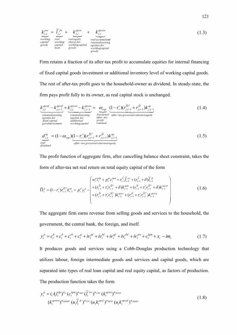
121
goodscapitalworkingforequitiesearningretained
daccumulatereal
eprew
tj
goodscapitalworking
forsharesequityreal
epsw
tj
loancapitalworkingreal
fw
tj
goodscapitalworking
pw
tj kklk ,,,,
~ (1.3)
Firm retains a fraction of its after-tax profit to accumulate equities for internal financing
of fixed capital goods investment or additional inventory level of working capital goods.
The rest of after-tax profit goes to the household-owner as dividend. In steady-state, the
firm pays profit fully to its owner, as real capital stock is unchanged.
equityonreturnrealgrosstaxafter
ep
tj
D
tjtj
i
t
retainedprofit
taxafteroffraction
rep
capitalworkingadditional
forequitiesearningretained
eprew
tj
eprew
tj
investmentgoodscapitalfixed
forequitiesearningretained
epref
tj
epref
tj krrkkkkp
1,
~
1,
~
1,1,,1,, ))(1( (1.4)
equityonreturnrealgrosstaxafter
ep
tj
D
tjtj
i
trep
dividendreal
vp
tj krrdp
1,
~
1,
~
1,, ))(1()1( (1.5)
The profit function of aggregate firm, after cancelling balance sheet constraint, takes the
form of after-tax net real return on total equity capital of the form
eprew
tt
i
t
D
t
epwc
tt
i
t
D
t
epref
tt
i
t
D
t
epfc
tt
i
t
D
t
fc
t
L
t
wc
t
L
t
igm
t
m
t
dp
t
p
t
p
t
d
t
ep
tt
i
t
p
t
krrkrr
krrkrr
lrlrcplw
ypkrpp
pp
p
1
~
1
~
11
~
1
~
1
1
~
1
~
11
~
1
~
1
1
~
11
~
1
1
~
1
)()(
)()(
~)(
~
)1(~
(1.6)
The aggregate firm earns revenue from selling goods and services to the household, the
government, the central bank, the foreign, and itself.
tt
igm
t
pw
t
cbf
t
gf
t
bf
t
pf
t
g
t
cb
t
b
t
h
t
p
t imxcivivivivivccccy
(1.7)
It produces goods and services using a Cobb-Douglas production technology that
utilizes labour, foreign intermediate goods and services and capital goods, which are
separated into types of real loan capital and real equity capital, as factors of production.
The production function takes the form
KEREFKESFLFCKEREW
KESWLWCMIGL
epref
tt
epsf
tt
fc
tt
eprew
t
epsw
t
wc
t
igm
t
dp
tt
p
t
kukuluk
klclAy
)()()~
()(
)()~
()()(
(1.8)
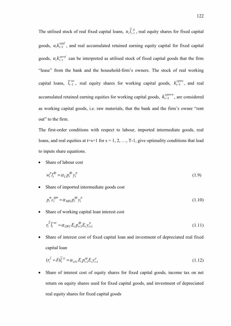
122
The utilised stock of real fixed capital loans, fc
tt lu 1
~ , real equity shares for fixed capital
goods, epsfttku 1 , and real accumulated retained earning equity capital for fixed capital
goods, epref
ttku 1 can be interpreted as utilised stock of fixed capital goods that the firm
―lease‖ from the bank and the household-firm‘s owners. The stock of real working
capital loans, ,~
1wc
tl real equity shares for working capital goods, epswtk 1 , and real
accumulated retained earning equities for working capital goods, eprewtk 1 , are considered
as working capital goods, i.e. raw materials, that the bank and the firm‘s owner ―rent
out‖ to the firm.
The first-order conditions with respect to labour, imported intermediate goods, real
loans, and real equities at t=s+1 for s = 1, 2, …, T-1, give optimality conditions that lead
to inputs share equations.
Share of labour cost
pt
dptL
dpt
pt yplw (1.9)
Share of imported intermediate goods cost
pt
dptMIG
igmt
mt ypcp (1.10)
Share of working capital loan interest cost
ptt
dpttLWC
wct
Lt yEpElr 11
~~ (1.11)
Share of interest cost of fixed capital loan and investment of depreciated real fixed
capital loan
p
tt
dp
ttLFC
fc
t
L
t yEpElr 11
~ ~)( (1.12)
Share of interest cost of equity shares for fixed capital goods, income tax on net
return on equity shares used for fixed capital goods, and investment of depreciated
real equity shares for fixed capital goods
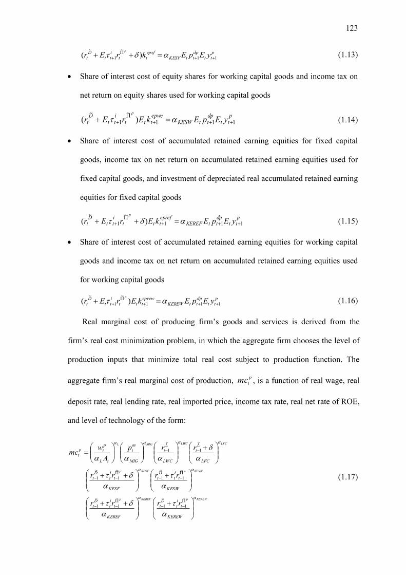
123
p
tt
dp
ttKESF
epsf
tt
i
tt
D
t yEpEkrErp
11
~
1
~
)(
(1.13)
Share of interest cost of equity shares for working capital goods and income tax on
net return on equity shares used for working capital goods
ptt
dpttKESW
epwcttt
itt
Dt yEpEkErEr
p
111
~
1
~
)(
(1.14)
Share of interest cost of accumulated retained earning equities for fixed capital
goods, income tax on net return on accumulated retained earning equities used for
fixed capital goods, and investment of depreciated real accumulated retained earning
equities for fixed capital goods
ptt
dpttKEREF
eprefttt
itt
Dt yEpEkErEr
p
111
~
1
~
)(
(1.15)
Share of interest cost of accumulated retained earning equities for working capital
goods and income tax on net return on accumulated retained earning equities used
for working capital goods
p
tt
dp
ttKEREW
eprew
ttt
i
tt
D
t yEpEkErErp
111
~
1
~
)(
(1.16)
Real marginal cost of producing firm‘s goods and services is derived from the
firm‘s real cost minimization problem, in which the aggregate firm chooses the level of
production inputs that minimize total real cost subject to production function. The
aggregate firm‘s real marginal cost of production, p
tmc , is a function of real wage, real
deposit rate, real lending rate, real imported price, income tax rate, real net rate of ROE,
and level of technology of the form:
KEREWpKEREFp
KESWpKESFp
LFCLWCMIGL
KEREW
t
i
t
D
t
KEREF
t
i
t
D
t
KESW
t
i
t
D
t
KESF
t
i
t
D
t
LFC
L
t
LWC
L
t
MIG
m
t
tL
p
tp
t
rrrr
rrrr
rrp
A
wmc
~
1
~
1
~
1
~
1
~
1
~
1
~
1
~
1
~
1
~
1
(1.17)
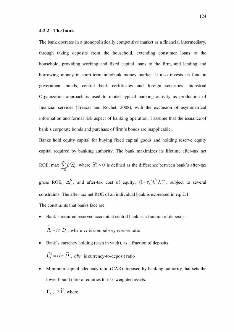
124
4.2.2 The bank
The bank operates in a monopolistically competitive market as a financial intermediary,
through taking deposits from the household, extending consumer loans to the
household, providing working and fixed capital loans to the firm, and lending and
borrowing money in short-term interbank money market. It also invests its fund in
government bonds, central bank certificates and foreign securities. Industrial
Organization approach is used to model typical banking activity as production of
financial services (Freixas and Rochet, 2008), with the exclusion of asymmetrical
information and formal risk aspect of banking operation. I assume that the issuance of
bank‘s corporate bonds and purchase of firm‘s bonds are inapplicable.
Banks hold equity capital for buying fixed capital goods and holding reserve equity
capital required by banking authority. The bank maximizes its lifetime after-tax net
ROE, max
0
~
t
b
t
t , where 0~
bt is defined as the difference between bank‘s after-tax
gross ROE, bt , and after-tax cost of equity,
eb
t
D
t
i
t Ki 1
~
1)1( , subject to several
constraints. The after-tax net ROE of an individual bank is expressed in eq. 2.4.
The constraints that banks face are:
Bank‘s required reserved account at central bank as a fraction of deposits.
tt DrrR~
, where rr is compulsory reserve ratio
Bank‘s currency holding (cash in vault), as a fraction of deposits.
t
b
t DcbrC~~
, cbr is currency-to-deposit ratio
Minimum capital adequacy ratio (CAR) imposed by banking authority that sets the
lower bound ratio of equities to risk-weighted assets.
~1,tj , where
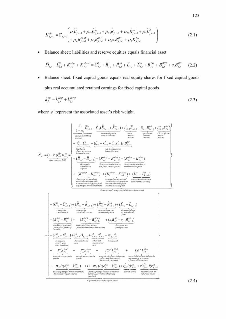
125
bfc
tj
BF
tjt
BG
tj
BCB
tj
ib
tj
xd
tjtj
b
tj
s
tj
tj
eb
tj
KBsBB
LRRCLK
1,71,61,51,4
1,31,221,211,201,1
1,1,
~~~
(2.1)
Balance sheet: liabilities and reserve equities equals financial asset
BF
tjt
BCB
tj
BG
tj
ib
tjtj
xd
tjtj
b
tj
ebrer
tj
ebsr
tj
ib
tktj BsBBLLRRCKKLD ,,,,,,,,,,,,
~~~~~
(2.2)
Balance sheet: fixed capital goods equals real equity shares for fixed capital goods
plus real accumulated retained earnings for fixed capital goods
ebref
tj
ebsf
tj
bfc
tj kkk ,,, (2.3)
where represent the associated asset‘s risk weight.
assetsinchangesandesExpenditur
equityonreturnnetontaxincome
eb
tjttj
i
t
equityofstco
eb
tjt
D
t
equitiesearningretainedbyfinanced
investmentnewgoodscapitalfixed
bfc
tj
bfc
tjtE
sharesequitybyfinancedinvestmentnewgoodscapitalfixed
bfc
tj
bfc
tjtE
incomebyfinancedinvestmenttreplacemen
goodscapitalfixedimported
bfcm
tj
m
t
incomebyfinancedinvestmenttreplacemen
goodscapitalfixeddomestic
bfcd
tj
d
t
goodsnconsumptioimported
bpm
tj
m
tj
goodsnconsumptiodomestic
bpd
tj
d
tj
stcolabour
b
tjtj
ostcnterestiloan
erbanktin
ib
tk
ib
tk
ostcnterestideposit
tj
D
tj
loannterbankitermshort
inchanges
ib
tj
ib
tj
assetsforeignnetinchanges
BF
tjt
BF
tjt
ncontractiomonetarypositiveecuritiessCBbuysbank
BCB
tj
BCB
tj
marketprimarygovtfrom
bondgovbuysbank
BG
tj
BG
tj
firmhouseholdto
loaninchanges
tjtj
depositsreservesexcessinchanges
xd
tj
xd
tj
reservesrequiredinchanges
tjtj
vaultincashinchanges
b
tj
b
tj
worthnetandsliabilitieinchangesandvenueseR
borrowingnterbankitermshortadditional
ib
tk
ib
tk
capitalequityreserveforearningsretained
equitiesearningretaineddaccumulateinchanges
ebrer
t
ebrer
t
investmentnewgoodscapitalfixedforearningsretained
equitiesearningretaineddaccumulateinchanges
ebref
t
ebref
t
capitalreservedforsharesequityinchanges
ebsr
tj
ebsr
tj
goodscapitalfixedforsharesequityinchanges
ebsf
tj
ebsf
tj
depositshousehold
inchanges
tjtj
incomenterestiassetsforeignnet
BF
tjttttt
incomenterestiloantermshort
terbankin
ib
tj
ib
tj
incomenteresti
escertificatCB
BCB
tj
cb
tj
incomenteresti
bondgov
BG
tj
g
tj
incomenteresti
loan
s
tj
L
tj
incomenterestidepositsreserve
xd
tjtj
R
t
incomeholdingcurrency
b
tj
t
t
ROEnettaxafter
eb
ttt
b
tj
kPikPikkPkkP
kPkPcPcP
lWLiDiLL
BsBsBBBB
LLRRRRCC
LLKKKK
KKKKDD
BsiiLi
BiBiLiRRiC
Ki
b
p
1,
~
1,1,
~
1
)(
1,,
)(
1,,
)(
1,
)(
1,,,,,
,,1,1,1,
~
1,1,,
1,1,
)(
1,,
)(
1,,
&
1,,1,,1,,1,,
1,,11
1,,1,,
'
1,,
1,
*
1
*
1
*
1
*
11,1,
1,1,1,1,1,
~
1,1,1,11,
1
~
1,
)()1()(
~~)
~~(
)()()(
)~~
()()()~~
(
)~~
()()(
)()()~~
(
)(~
~)(
~
1
)1(~
(2.4)
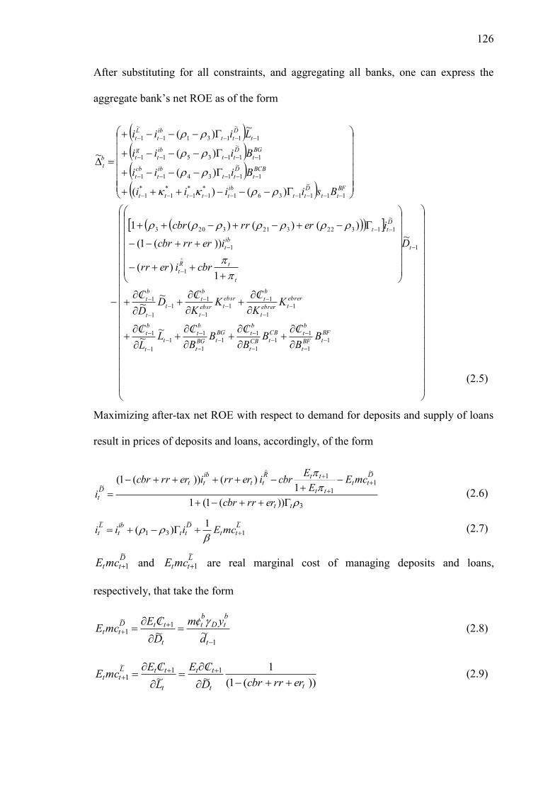
126
After substituting for all constraints, and aggregating all banks, one can express the
aggregate bank‘s net ROE as of the form
BF
tBF
t
b
tCB
tCB
t
b
tBG
tBG
t
b
tt
t
b
t
ebrer
tebrer
t
b
tebsr
tebsr
t
b
tt
t
b
t
t
t
tR
t
ib
t
D
tt
BF
tt
D
tt
ib
ttttt
BCB
t
D
tt
ib
t
cb
t
BG
t
D
tt
ib
t
g
t
t
D
tt
ib
t
L
t
b
t
BB
CB
B
CB
B
CL
L
C
KK
CK
K
CD
D
C
D
cbrierrr
ierrrcbr
ierrrcbr
Bsiiii
Biii
Biii
Liii
1
1
11
1
11
1
11
1
1
1
1
11
1
11
1
1
1
1
1
~
113223213203
11
~
11361
*
1
*
1
*
1
*
1
1
~
113411
1
~
113511
1
~
11311
~
1
~~
~~
~
1)(
))(1(
)()()(1
)()(
)(
)(
~)(
~
(2.5)
Maximizing after-tax net ROE with respect to demand for deposits and supply of loans
result in prices of deposits and loans, accordingly, of the form
3
~
1
1
1
~
))(1(1
1)())(1(
tt
Dtt
tt
ttRtt
ibtt
Dt
errrcbr
mcEE
Ecbrierrrierrrcbr
i
(2.6)
Ltt
Dtt
ibt
Lt mcEiii
~
1
~
31
~ 1)(
(2.7)
DttmcE~
1 and LttmcE~
1 are real marginal cost of managing deposits and loans,
respectively, that take the form
1
1~
1 ~~
t
btD
bt
t
ttDtt
d
ycm
D
CEmcE
(2.8)
))(1(
1~~
11~
1
tt
tt
t
ttLtt
errrcbrD
CE
L
CEmcE
(2.9)
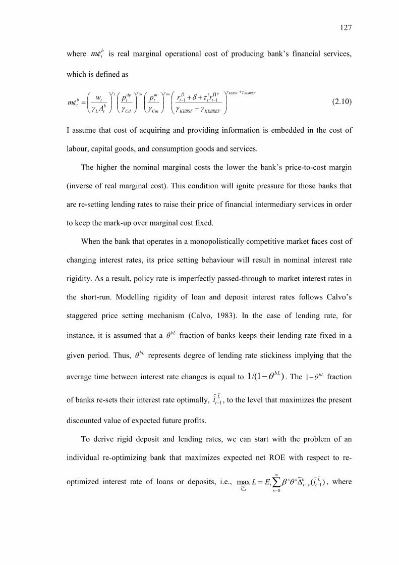
127
where b
tcm is real marginal operational cost of producing bank‘s financial services,
which is defined as
KEBREFKEBSFpCmCdL
KEBREFKEBSF
t
i
t
D
t
Cm
m
t
Cd
dp
t
b
tL
tb
t
rrpp
A
wcm
~
1
~
1
(2.10)
I assume that cost of acquiring and providing information is embedded in the cost of
labour, capital goods, and consumption goods and services.
The higher the nominal marginal costs the lower the bank‘s price-to-cost margin
(inverse of real marginal cost). This condition will ignite pressure for those banks that
are re-setting lending rates to raise their price of financial intermediary services in order
to keep the mark-up over marginal cost fixed.
When the bank that operates in a monopolistically competitive market faces cost of
changing interest rates, its price setting behaviour will result in nominal interest rate
rigidity. As a result, policy rate is imperfectly passed-through to market interest rates in
the short-run. Modelling rigidity of loan and deposit interest rates follows Calvo‘s
staggered price setting mechanism (Calvo, 1983). In the case of lending rate, for
instance, it is assumed that a bL fraction of banks keeps their lending rate fixed in a
given period. Thus, bL represents degree of lending rate stickiness implying that the
average time between interest rate changes is equal to )1/(1 bL . The bL1 fraction
of banks re-sets their interest rate optimally, L
ti~
1
, to the level that maximizes the present
discounted value of expected future profits.
To derive rigid deposit and lending rates, we can start with the problem of an
individual re-optimizing bank that maximizes expected net ROE with respect to re-
optimized interest rate of loans or deposits, i.e.,
0
~
1ˆ
)(~
max~
1 s
L
t
b
st
ss
ti
iELL
t
, where
128
)(~ ~
1
L
t
b
stt iE
is the bank‘s net ROE at t+1+s, given that it re-optimizes its interest rate to
be equal to L
ti~
1
at the end of t-1 and keep it fixed to t-1+s. After some algebra, we can
find rigid interest rate of deposits and loans in deviation from their corresponding
steady-state values of the form:
tD
ttD
Dbtt
DDDtt
DDt
D
D
Dt
E
CMEiEii
ˆ)1(ˆ)1(
ˆ)1)(1(ˆˆ
1
1ˆ
1
~
1
~
1
~
1
2
~
(2.11)
where:
33 )(11ln)(11lnˆ rrcrerrrcr ttt
Lbtt
LLLtt
LLt
L
L
Lt CMEiEii
~
1
~
1
~
12
~ˆ)1)(1(ˆˆ
1
1ˆ
(2.12)
LbtCM
~ˆ and
DbtCM
~ˆ are marginal cost of loans and deposits in deviation from steady-state,
respectively, where
Dib
Dtt
tt
ttibtt
Dbt
mccbrirrcr
mcEE
EcbrierrrcrCM
~
~
1
1
1~
1))(1(ln
1))(1(lnˆ
(2.13)
LDibL
tt
D
tt
ib
t
Lb
t mciimcEiiCM~~
31
~
1
~
31
~
)(ln)(lnˆ (2.14)
We further need to find after-tax net real ROE and maximise its lifetime values
subject to the bank‘s services output (b
ty ). It solves for the demand for deposits, labour,
capital goods and consumption goods and services that the bank utilise in
intermediating fund.
Recent researches on banking in DGE models use loan supply functions instead of
bank‘s production function of loan services. One of them is Goodfriend & McCallum
(2007) that applies a real loan ‗production‘ function relating to management of loans, by
129
a combination of collateral, tk , and loan monitoring db
tl . Loan supply function is of the
form
1
2131 )()(~ db
ttt
k
ttt
s
t lAkpAbFl , where 131 t
k
ttt kpAb is collateral, with
)1(11
B
t
t
tt R
P
Bb
is real bonds, and ktp is the real price of capital goods.
Leao & Leao (2006) defines real loan ‗production‘ function as a measure of how
much credit, in real terms, that the banks can produce for each combination of work
hours hired )( db
tl and capital stock available )( b
tk . This ‗production‘ function can be
summarized by a Cobb-Douglas type of technology of the form db
t
b
tt
s
t lkAl
1~
.
Another type of loan supply function assumes a linear loan technology, in which
deposits are assumed to be convertible into loans with a linear technology (Gerali, et.al,
2008). In this setting, banks deposits are essentially an input to the loan supply process.
Nominal supply of loans, )~
( tL , is a function of household deposits fund, )~
( tD , central
bank loans to the bank )( tM and bank‘s equities )( fb
tK ; the function takes the form of
),~
(~ fb
tttt KMDfL . Similar with this approach is the intermediation technology for
loan production, )~
(~
tttt XDL , where tX is a lump-sum nominal transfer from the
monetary authority, and ]1,0[t represents the fraction of total deposits lent out to the
firm (Atta-Mensah & Dib, 2008).
In this study, I interpret the stock of real loans as ―good‘s production power of
loans‖, which are transferred from the surplus unit households, through its supply of
real deposits, to the deficit unit‘s households and firms. Real loans can stand for the
number of goods and services that households can purchase by borrowing consumption
loans. In the form of working and fixed capital loans extended to the firm, their real
130
value means the quantity of working and fixed capital goods that the firm can buy to
produce goods and services.
Real deposit is ―goods‘ and services‘ consumption power of deposit money‖ that
the household, as the surplus unit agent, gives up by putting some amount of fund in
their bank account. The bank transfers the purchasing power of deposit fund to other
households and the firm through the bank‘s placement of fund on loans. It can also
transfer it to the government through bank‘s purchase of government bonds that enable
the government to finance fixed capital goods investment. When the bank uses part of
deposit funds to buy central bank certificates or to fulfill required reserve ratio,
monetary authority shrinks some amount of money. In real terms, it implies that the
central bank eliminates goods purchasing or producing power of some loanable funds. It
is the lost of opportunity to produce consumption, intermediate and capital goods
through lending and financing government deficit.
The bank‘s output is financial intermediation services. Given the interpretation of
real loans and real deposits, we can construe the bank‘s output in real term as
―intermediation services of leased goods‖. It is as if banks lease goods from the
household and rent them out to other households as consumption goods, to the firm as
working and fixed capital goods, to the government as fixed capital goods, and to the
central bank as all type of goods. This framework links banking sector, which deals
with stock and nominal variables, with real sector that is in flow and real variables.
Demand for the bank‘s real output of financial intermediary services is the sum of
interest payment to the bank. Interest payment consists of households‘ and firms‘ real
interest payment for outstanding loans (household‘s and firm‘s consumption of bank
services), and the government and the central bank consumption of bank services in
terms of real interest payment of government bonds and central bank certificates.
131
bt
t
txdtt
Rt
BFtttttt
BCBt
cbt
BGt
gtt
Lt
bt
dbt
crrr
bqrrbrbrlryp
1111
1*
1*
1*
1*
111111
~
1
~1
)(
)(~
(2.15)
I assume that the bank‘s real financial services is produced using a Cobb-Douglas type
production technology of the form
KEBREFKEBSFKEBRERKEBSRDCmCdL ebref
t
ebsf
t
ebrer
t
ebsr
tt
bm
t
bd
t
b
t
b
t
b
t kkkkdcclAy
11111
~ (2.16)
Input for producing financial intermediary services consists of real deposits ( 1
~td ),
effective labour working time (db
t
b
t lA ), domestic consumption goods and services )(bdtc
, imported consumption goods and services (bm
tc ), real accumulated retained earning
equities for fixed capital goods (ebref
tk 1 ), real equity shares for fixed capital goods (ebsf
tk 1
), real equity shares for reserve capital (ebsr
tk 1 ) and real accumulated retained earning
equities for reserve capital (ebrer
tk 1 ). The first input resembles the ―goods‖ that the bank
leases from the household. The last two inputs are analogous to the ―goods‘ inventory‖
that is required to safeguard the continuity of financial services production. The other
inputs offer the same services as in the firm‘s production function. The bank chooses
the level of factor inputs that maximize its present discounted values of lifetime after-
tax net real ROE,
0
~
t
b
t
t
tE
equitiessliabilitieassetsfinancialmanagingofstcorrcbbblkkdc
ebreft
ebsftt
it
bDt
bpmt
mt
bpdt
dpt
btt
ebrert
ebsrtt
it
Dtt
Dt
yp
xdtt
Rt
bt
t
t
BFtttttt
BCBt
cbt
BGt
gt
st
Lt
bt
xdtt
bt
BFt
BCBt
BGt
st
ebrert
ebsrt
dtt
b
b
bt
dbt
kkrrcpcplw
kkrrdr
rrrc
bqrrbrbrlr
&,),,~,,,,
~,,,
~(
11
~
1
~
1
11
~
1
~
11
~
1
1111
1*
1*
1*
1*
111111
~
1
1111111111
))((
))((~
)(~1
)(~
~
(2.17)
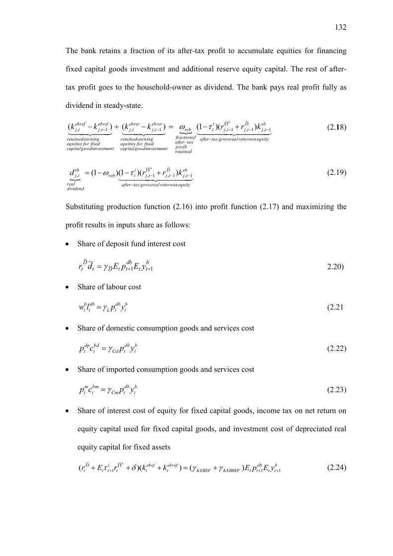
132
The bank retains a fraction of its after-tax profit to accumulate equities for financing
fixed capital goods investment and additional reserve equity capital. The rest of after-
tax profit goes to the household-owner as dividend. The bank pays real profit fully as
dividend in steady-state.
equityonreturnrealgrosstaxafter
eb
tj
D
tjtj
i
t
retainedprofit
taxafteroffraction
reb
investmentgoodscapitalfixedforequities
earningretained
ebrer
tj
ebrer
tj
investmentgoodscapitalfixedforequities
earningretained
ebref
tj
ebref
tj krrkkkkb
1,
~
1,
~
1,1,,1,, ))(1()()( (2.18)
equityonreturnrealgrosstaxafter
eb
tj
D
tjtj
i
treb
dividendreal
vb
tj krrdb
1,
~
1,
~
1,, ))(1()1( (2.19)
Substituting production function (2.16) into profit function (2.17) and maximizing the
profit results in inputs share as follows:
Share of deposit fund interest cost
btt
dbttDt
Dt yEpEdr 11~
~ ~ 2.20)
Share of labour cost
b
t
db
tL
db
t
b
t yplw (2.21
Share of domestic consumption goods and services cost
b
t
db
tCd
bd
t
dp
t ypcp (2.22)
Share of imported consumption goods and services cost
b
t
db
tCm
bm
t
m
t ypcp (2.23)
Share of interest cost of equity for fixed capital goods, income tax on net return on
equity capital used for fixed capital goods, and investment cost of depreciated real
equity capital for fixed assets
b
tt
db
ttKEBREFKEBSF
ebref
t
ebsf
tt
i
tt
D
t yEpEkkrErb
11
~
1
~
)())((
(2.24)
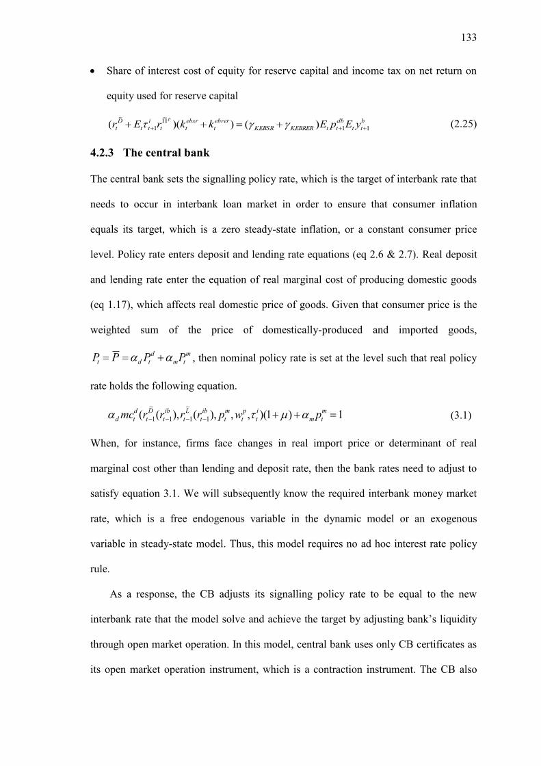
133
Share of interest cost of equity for reserve capital and income tax on net return on
equity used for reserve capital
b
tt
db
ttKEBRERKEBSR
ebrer
t
ebsr
tt
i
tt
D
t yEpEkkrErp
11
~
1
~
)())((
(2.25)
4.2.3 The central bank
The central bank sets the signalling policy rate, which is the target of interbank rate that
needs to occur in interbank loan market in order to ensure that consumer inflation
equals its target, which is a zero steady-state inflation, or a constant consumer price
level. Policy rate enters deposit and lending rate equations (eq 2.6 & 2.7). Real deposit
and lending rate enter the equation of real marginal cost of producing domestic goods
(eq 1.17), which affects real domestic price of goods. Given that consumer price is the
weighted sum of the price of domestically-produced and imported goods,
m
tm
d
tdt PPPP , then nominal policy rate is set at the level such that real policy
rate holds the following equation.
1)1)(,,),(),(( 1
~
11
~
1
m
tm
i
t
p
t
m
t
ib
t
L
t
ib
t
D
t
d
td pwprrrrmc (3.1)
When, for instance, firms face changes in real import price or determinant of real
marginal cost other than lending and deposit rate, then the bank rates need to adjust to
satisfy equation 3.1. We will subsequently know the required interbank money market
rate, which is a free endogenous variable in the dynamic model or an exogenous
variable in steady-state model. Thus, this model requires no ad hoc interest rate policy
rule.
As a response, the CB adjusts its signalling policy rate to be equal to the new
interbank rate that the model solve and achieve the target by adjusting bank‘s liquidity
through open market operation. In this model, central bank uses only CB certificates as
its open market operation instrument, which is a contraction instrument. The CB also
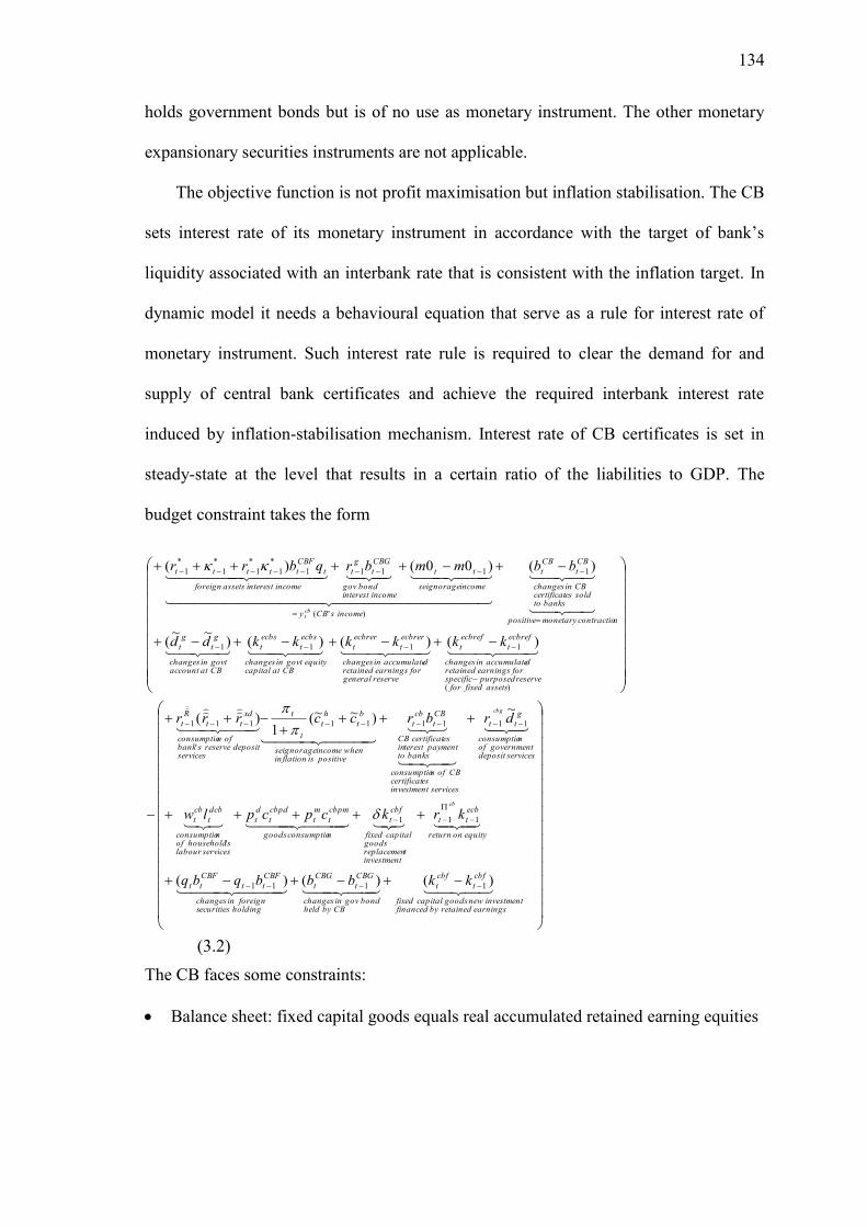
134
holds government bonds but is of no use as monetary instrument. The other monetary
expansionary securities instruments are not applicable.
The objective function is not profit maximisation but inflation stabilisation. The CB
sets interest rate of its monetary instrument in accordance with the target of bank‘s
liquidity associated with an interbank rate that is consistent with the inflation target. In
dynamic model it needs a behavioural equation that serve as a rule for interest rate of
monetary instrument. Such interest rate rule is required to clear the demand for and
supply of central bank certificates and achieve the required interbank interest rate
induced by inflation-stabilisation mechanism. Interest rate of CB certificates is set in
steady-state at the level that results in a certain ratio of the liabilities to GDP. The
budget constraint takes the form
earningsretainedbyfinancedinvestmentnewgoodscapitalfixed
cbf
t
cbf
t
CBbyheldbondgovinchanges
CBG
t
CBG
t
holdingecuritiessforeigninchanges
CBF
tt
CBF
tt
equityonreturn
ecb
tt
investmenttreplacemen
goodscapitalfixed
cbf
t
nconsumptiogoods
cbpm
t
m
t
cbpd
t
d
t
serviceslabourshouseholdof
nconsumptio
dcb
t
cb
t
servicesdepositgovernmentof
nconsumptio
g
tt
servicesinvestmentescertificat
CBofnconsumptio
bankstopaymentterestin
escertificatCB
CB
t
cb
t
positiveisflationinwhenincomeseignorage
b
t
h
t
t
t
servicesdepositreservesbank
ofnconsumptio
xd
tt
R
t
assetsfixedforreservepurposedspecific
forearningsretaineddaccumulateinchanges
ecbref
t
ecbref
t
reservegeneralforearningsretained
daccumulateinchanges
ecbrer
t
ecbrer
t
CBatcapitalequitygovtinchanges
ecbs
t
ecbs
t
CBataccountgovtinchanges
g
t
g
t
ncontractiomonetarypositive
bankstosoldescertificatCBinchanges
CB
t
CB
t
incomesCBy
incomeseignorage
tt
incomenterestibondgov
CBG
t
g
t
incomenterestiassetsforeign
t
CBF
ttttt
kkbbbqbq
krkcpcplw
drbrccrrr
kkkkkkdd
bbmmbrqbrr
cb
cbg
cbt
)()()(
~)~~(
1)(
)()()()~~
(
)()00()(
1111
111
'
111111
'
111
)(
1111
1
)'(
1111
*
1
*
1
*
1
*
1
(3.2)
The CB faces some constraints:
Balance sheet: fixed capital goods equals real accumulated retained earning equities
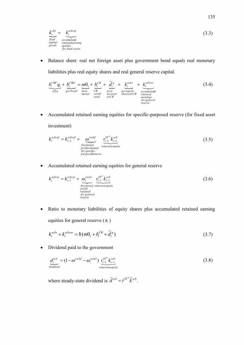
135
assetsfixedforequities
earningretaineddaccumulate
ecbref
t
goodscapitalfixed
cbf
t kk (3.3)
Balance sheet: real net foreign asset plus government bond equals real monetary
liabilities plus real equity shares and real general reserve capital.
reservegeneralfor
earningsretained
daccumulate
ecbrer
t
CBatsharesequitygov
ecbs
t
CBataccountgovt
g
t
catescertifiCB
CB
t
moneybase
t
bondgov
CBG
t
NFA
t
CBF
t kkdbmbqb
~0
(3.4)
Accumulated retained earning equities for specific-purposed reserve (for fixed asset
investment)
equityonreturn
ecb
tt
reservepurposedspecificfor
retainedprofitoffraction
recbfecbref
t
ecbref
t krkkcb
111
(3.5)
Accumulated retained earning equities for general reserve
equityonreturn
ecb
tt
reservegeneralfor
retainedprofit
offraction
recbr
t
ecbrer
t
ecbrer
t krkkcb
111
(3.6)
Ratio to monetary liabilities of equity shares plus accumulated retained earning
equities for general reserve ( )
)~
0( g
t
CB
tt
ecbrer
t
ecbs
t dbmkk
(3.7)
Dividend paid to the government
equityonreturn
ecb
tt
recbr
t
recbf
dividend
vcb
t krdcb
11)1(
(3.8)
where steady-state dividend is ecbvcb krd
cb .
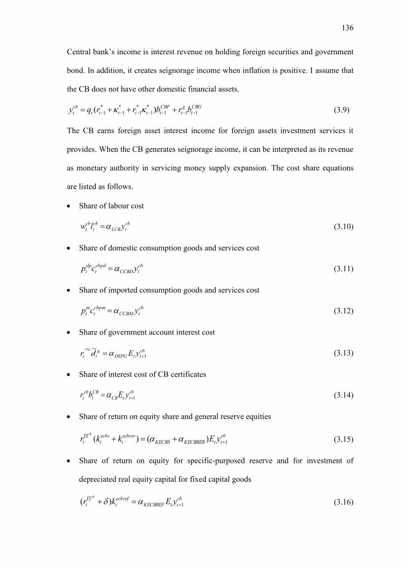
136
Central bank‘s income is interest revenue on holding foreign securities and government
bond. In addition, it creates seignorage income when inflation is positive. I assume that
the CB does not have other domestic financial assets.
CBG
t
g
t
CBF
tttttt
cb
t brbrrqy 111
*
1
*
1
*
1
*
1 )(
(3.9)
The CB earns foreign asset interest income for foreign assets investment services it
provides. When the CB generates seignorage income, it can be interpreted as its revenue
as monetary authority in servicing money supply expansion. The cost share equations
are listed as follows.
Share of labour cost
cb
tLCB
cb
t
cb
t ylw (3.10)
Share of domestic consumption goods and services cost
cb
tCCBD
cbpd
t
dp
t ycp (3.11)
Share of imported consumption goods and services cost
cb
tCCBM
cbpm
t
m
t ycp (3.12)
Share of government account interest cost
cb
ttDEPG
g
tt yEdrcbg
1
~ (3.13)
Share of interest cost of CB certificates
cb
ttCB
CB
t
cb
t yEbr 1 (3.14)
Share of return on equity share and general reserve equities
cb
ttKECBRERKECBS
ecbrer
t
ecbs
tt yEkkrcb
1)()(
(3.15)
Share of return on equity for specific-purposed reserve and for investment of
depreciated real equity capital for fixed capital goods
cb
ttKECBREF
ecbref
tt yEkrcb
1)(
(3.16)
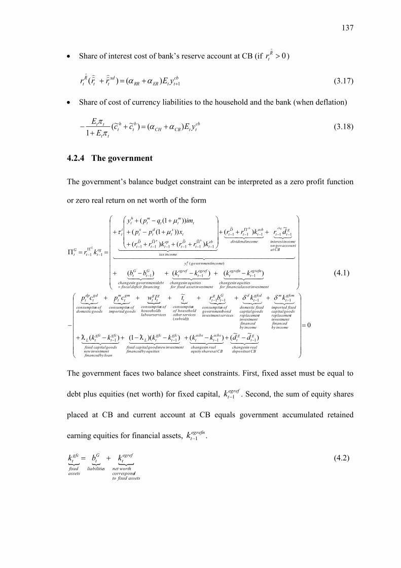
137
Share of interest cost of bank‘s reserve account at CB (if 0R
tr
)
cb
ttERRR
xd
tt
R
t yErrr 1)()(
(3.17)
Share of cost of currency liabilities to the household and the bank (when deflation)
cb
ttCBCH
b
t
h
t
tt
tt yEccE
E)()~~(
1
(3.18)
4.2.4 The government
The government‘s balance budget constraint can be interpreted as a zero profit function
or zero real return on net worth of the form
0
)~~
()())(1()(
~
)()()(
~)(
)()(
))1((
))1((
1111
1111
)(
'
111
)(
1111
~
1
1
~
1
~
11
~
1
~
1
11
CBatdepositsrealinchanges
g
t
g
t
CBatsharesequityrealinchanges
ecbs
t
ecbs
t
equitiesbyfinancedinvestmentnewgoodscapitalfixed
gfc
t
gfc
tL
loanbyfinancedinvestmentnew
goodscapitalfixed
gfc
t
gfc
tL
incomebyfinancedinvestment
treplacemengoodscapital
fixedimported
gfcm
t
m
incomebyfinancedinvestment
treplacemengoodscapital
fixeddomestic
gfcd
t
d
servicesinvestmentbondgovernmentofnconsumptio
G
t
g
t
subsidyservicesother
householdofnconsumptio
t
serviceslabourshousehold
ofnconsumptio
g
t
g
t
goodsimportedofnconsumptio
gm
t
m
t
goodsdomesticofnconsumptio
gd
t
dp
t
investmentassetfinancialforequitiesinchanges
egrefn
t
egrefn
t
investmentassetfixedforequitiesinchanges
egref
t
egref
t
financingdeficitfiscaldebtgovernmentinchanges
G
t
G
t
incomegovernmenty
CBataccountgovonincomenteresti
g
tt
incomedividend
ecb
tt
D
t
incometax
eb
tt
D
t
ep
tt
D
t
t
x
t
d
t
x
t
t
m
tt
m
t
h
t
i
t
eg
tt
G
t
ddkkkkkk
kkbrtlwcpcp
kkkkbb
drkrr
krrkrr
xpp
imqpy
kr
gt
cbgcb
bp
G
(4.1)
The government faces two balance sheet constraints. First, fixed asset must be equal to
debt plus equities (net worth) for fixed capital, egref
tk 1 . Second, the sum of equity shares
placed at CB and current account at CB equals government accumulated retained
earning equities for financial assets, egrefn
tk 1 .
assetsfixedtoscorrespond
worthnet
egref
t
sliabilitie
G
t
assetsfixed
gfc
t kbk (4.2)
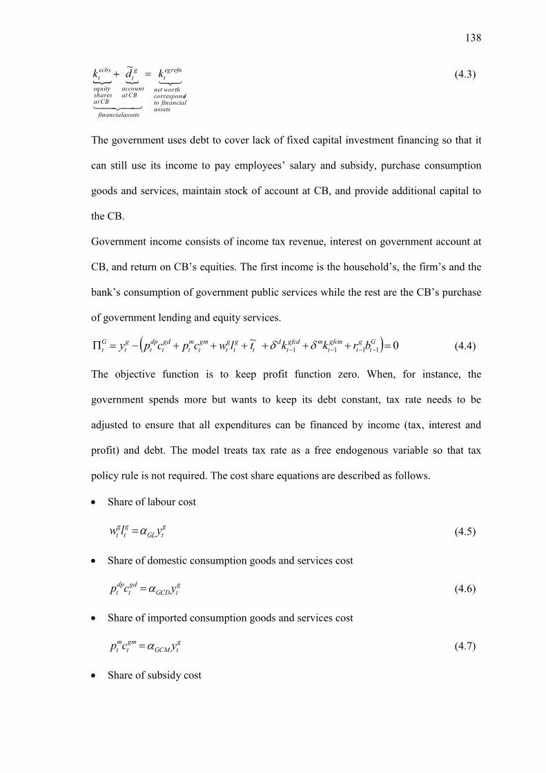
138
assetsfinancialto
scorrespondworthnet
egrefn
t
assetsfinancial
CBataccount
g
t
CBatsharesequity
ecbs
t kdk ~
(4.3)
The government uses debt to cover lack of fixed capital investment financing so that it
can still use its income to pay employees‘ salary and subsidy, purchase consumption
goods and services, maintain stock of account at CB, and provide additional capital to
the CB.
Government income consists of income tax revenue, interest on government account at
CB, and return on CB‘s equities. The first income is the household‘s, the firm‘s and the
bank‘s consumption of government public services while the rest are the CB‘s purchase
of government lending and equity services.
0~
1111
G
t
g
t
gfcm
t
mgfcd
t
d
t
g
t
g
t
gm
t
m
t
gd
t
dp
t
g
t
G
t brkktlwcpcpy
(4.4)
The objective function is to keep profit function zero. When, for instance, the
government spends more but wants to keep its debt constant, tax rate needs to be
adjusted to ensure that all expenditures can be financed by income (tax, interest and
profit) and debt. The model treats tax rate as a free endogenous variable so that tax
policy rule is not required. The cost share equations are described as follows.
Share of labour cost
g
tGL
g
t
g
t ylw (4.5)
Share of domestic consumption goods and services cost
g
tGCD
gd
t
dp
t ycp (4.6)
Share of imported consumption goods and services cost
g
tGCM
gm
t
m
t ycp (4.7)
Share of subsidy cost
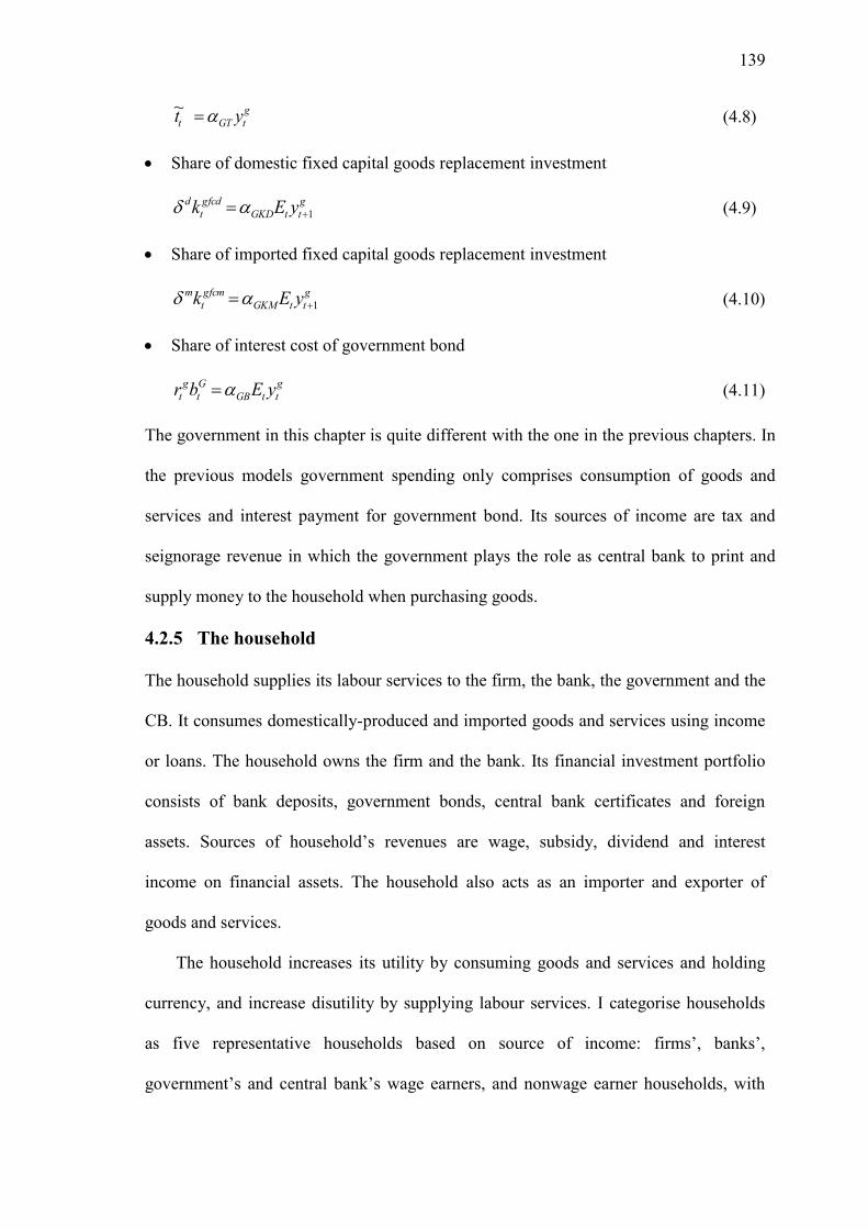
139
g
tGTt yt ~
(4.8)
Share of domestic fixed capital goods replacement investment
g
ttGKD
gfcd
t
d yEk 1 (4.9)
Share of imported fixed capital goods replacement investment
g
ttGKM
gfcm
t
m yEk 1 (4.10)
Share of interest cost of government bond
g
ttGB
G
t
g
t yEbr (4.11)
The government in this chapter is quite different with the one in the previous chapters. In
the previous models government spending only comprises consumption of goods and
services and interest payment for government bond. Its sources of income are tax and
seignorage revenue in which the government plays the role as central bank to print and
supply money to the household when purchasing goods.
4.2.5 The household
The household supplies its labour services to the firm, the bank, the government and the
CB. It consumes domestically-produced and imported goods and services using income
or loans. The household owns the firm and the bank. Its financial investment portfolio
consists of bank deposits, government bonds, central bank certificates and foreign
assets. Sources of household‘s revenues are wage, subsidy, dividend and interest
income on financial assets. The household also acts as an importer and exporter of
goods and services.
The household increases its utility by consuming goods and services and holding
currency, and increase disutility by supplying labour services. I categorise households
as five representative households based on source of income: firms‘, banks‘,
government‘s and central bank‘s wage earners, and nonwage earner households, with
140
the assumption that each household has a unique source of income. Each representative
household has a utility function in the form of a constant elasticity of substitution
function. The period utility function of the household-firms‘ worker takes the form
f
f
tlf
hf
tfc
hf
tcff
t
hf
t
hf
t
hf
t
f
lcclccu
11
~
1),~,(
11
~
1
(5.1)
Parameter , which is the intertemporal elasticity of consumption or real interest rate
elasticity of consumption, can be unique if each household is assumed to have identical
preference on consuming goods and services in an aggregate goods market. We can
apply the same assumption to , which is nominal interest rate elasticity of currency
demand, because each household is assumed behaving uniformly in holding currency
supplied by central bank. However, it is not the case with , which is real wage
elasticity of labour supply. While each household, regardless where they work at, has
the same leisure preference )( l they supply their labour services to four labour markets
that have different labour demand characteristics depending on their corresponding
income and labour share parameter (wage budget). Consequently, we can no longer
have the assumption of single aggregate wage and sole elasticity of labour supply with
respect to real wage. Firms, banks, government and central bank have different income
and share of income that goes to labour cost. That justifies the need for having
heterogenous households in this model.
The household faces balance sheet constraint that equalise real wealth and real loan
with physical and financial assets.
pl
t
pw
t
h
t
h
t
eb
t
ep
t
HF
tt
HCB
t
HG
t
FH
tt
c
tt aadckkbqbbbqlw ~~~~
(5.2)
It maximises its utility subject to budget constraint (5.3) that ensures that its
consumption and investment can be financed by income, borrowing and saving. The
first order conditions with respect to (1) real current and future consumption, (2)
141
demand for real currency, (3) supply of labour, (4) real imported goods, (5) real
deposits, (6) real government bonds, (7) real central bank certificates, (8) real foreign
bonds, (9) nominal foreign bonds, (10) real domestic consumption loans, at t=s+1, for
s=1,2,...,T-1, give the optimality conditions that are required to get household‘s
behavioural equations.
)(
1
)(
1
)(
1111
1111
),
(
11
*
11
*
11
~
1
111
)(
1
'''
''
'
11
*
1
*
1
*
1
*
111111
~
1
)()(
)~~
()~~()()(
)()()(
)(~
)()~~
()~~(
))1(())1((
~
1)(
~
~
loanbyfinancednconsumptiogoods
debtbyfinancedassetsphysical
inchanges
pl
t
pl
t
savingbyfinancednconsumptiogoods
savingbyfinancedassetsphysical
inchanges
pw
t
pw
t
investmentassetfinancialassetsfinancialinchanges
h
t
h
t
h
t
h
t
ebs
t
ebs
t
eps
t
eps
t
HF
tt
HF
tt
HCB
t
HCB
t
HG
t
HG
t
ostc
ypayment
taxincomeservicespublic
governmentofnconsumptio
h
t
i
t
servicesloanforeignofnconsumptio
FH
tttttt
servicesloannconsumptio
domesticofnconsumptio
c
t
L
t
incomebyfinancedgoods
importedofnconsumptio
hpm
t
m
t
incomebyfinancedgoods
domesticofnconsumptio
hpd
t
dp
t
loannconsumptioinchanges
FH
tt
FH
tt
c
t
c
t
savingwealthinchanges
tt
yincome
incomeprofitsxportere
t
x
t
d
t
x
t
incomeprofitsimporter
t
m
tt
m
t
incomedividendsowner
sbankandsfirm
vb
t
vp
t
incometerestinsassetfinancial
h
t
t
tHF
tttttt
HCB
t
cb
t
HG
t
g
tt
D
t
incomesubsidy
t
incomewage
cb
t
cb
t
g
t
g
t
b
t
b
t
f
t
f
t
aaaa
ddcckkkk
bqbqbbbb
ybqrrlrcpcp
bqbqllww
xppimqpdd
cbqrrbrbrdr
tlwlwlwlw
taxht
ht
(5.3)
Labour supply
The household‘s supply of working hours to the firm, bank, central bank and
government is derived by combining the optimality condition with respect to the
consumption of each corresponding worker‘s group and to the supply of labour to the
corresponding employer. Labour supply of nonemployee‘s households is set as a certain
percentage of total employment. The example of household‘s labour supply to the firm
takes the form
142
f
hftlf
ft
itcff
t
c
wl
1
)1(
(5.4)
Consumption
The first-order condition of utility maximization with respect to the current and future
consumption, and the first order condition with respect to real deposits, provides the
Euler condition for the intertemporal consumption allocation of five groups of
households, both for consumption of domestic and imported goods and services. For the
household-firm‘s worker, for example, the consumption equations take the form of
1
1
~
11
))1(1(
dtt
dt
Dt
itthpdf
tthpdft
pE
prEcEc
(5.5)
1
1
~
11
))1(1(
mtt
mt
Dt
itthpmf
tthpmft
pE
prEcEc
(5.6)
Currency demand
Demand for currency for five household‘s group are derived by combining the first-
order condition of the household‘s utility maximization with respect to real
consumption, real currency demand, and real domestic bonds, and the definition of real
interest rate, 1
~
1~
11
)1(1)1(1
tt
Dt
ittD
titt
E
iErE
. The household-firms worker‘s demand
for currency takes the form:
1
~
1~
11
~
1/
))1(1(
)1(~
Dt
ittfc
ttitt
Dt
ittcfhf
thf
t
iE
EEiEcc
(5.7)
Cost structure
143
We can reconcile household income and cost with utility maximisation to result in time-
varying coefficients of cost share as follows.
Coefficient of share of domestic consumption goods and services cost
h
t
hpd
t
dp
tHDt
y
cp
` (5.8)
Coefficient of share of imported consumption goods and services cost
h
t
hpm
t
m
tHMt
y
cp
(5.9)
The time-varying coefficients of shares of domestic and imported consumption goods
and services ( HDt and HMt ) depend on the sum of demand for consumption goods
provided by consumption Euler equation, household‘s income, and the price of domestic
and imported goods.
Coefficient of share of income tax payment. It is equal to income tax rate.
i
th
t
taxh
tHTt
y
y
(5.10)
Coefficient of share of interest cost of foreign loans
)1( HTtHMtHDtHFHFt (5.11)
where HF is a fixed ratio of foreign consumption loan to total consumption loan
Coefficient of share of interest cost of domestic consumption loans
)1)(1( HTtHMtHDtHFHLt (5.12)
The household‘s demand for real consumption loan is given by L
t
h
ttHLtc
tr
yEl ~
~ . While
demand for and supply of real loan clear in steady-state, they do not necessarily the case
in a dynamic state. The bank‘s loan interest income for loan services to the firm and
household is determined by loan supply.
144
4.3 Cost push vs. demand pull inflation
Inflation is a rise in the general level of prices of goods and services over a period of
time. In a simpler definition, inflation is an identity equation of an increase in the
general price level. Sellers set and ask price. Buyers bid and pay the price. Thus, I
analyse inflation determinants through price determinants analysis using basic price
equation: )1( p
t
p
t
d
t MCP . It is the price of domestically-produced goods and
services, which has only two main determinants: marginal cost and marginal profit.
I use old macroeconomic concept: cost-push and demand-pull inflation. Cost-push
inflation occurs when sellers respond to a rising cost by increasing their prices to protect
profit margin. Demand-pull inflation occurs through upward adjustment of profit
margin as the seller‘s respond to a rising demand. Profit margin is measured by net rate
of return on equity.
One might ask where other measures of inflation determinants such as administered
price shocks and people‘s expectation of inflation, which is the one that central banks
have placed considerable emphasise, have places in this classic concept. Shocks to the
administered price of domestically produced consumer goods and services can be partly
categorised as demand-pull and cost-push inflation. For instance, in the case of shock to
the administered transportation fuel price, price increases can affect both demand for
and cost of transportation services. However, the new nonequilibrium price is fully
transmitted to consumer price basket without entering agent‘s consumption decision and
production cost calculation process. This controlled price does not exist in this model as
all goods price is the equilibrium price of supply of and demand for goods and services.
Price expectation is already inherent in demand-pull and cost-push inflation
framework. Sellers‘ calculation of marginal cost must take the expectation (forecast) of
input prices into consideration. When they set prices of their products to be kept fixed
145
for t periods ahead, they need to consider the expectation of input prices that will occur
during the corresponding horizon. Consumers also consider their expectation of future
price of consumption goods and services in their consumption decision as it depends on
expected future consumption (see equation 5.5-5.6).
4.3.1 Cost-push inflation
Analysis of cost-push inflation uses marginal cost in real term with marginal profit is
expressed as the ratio of after-tax net ROE to total cost. Real marginal cost depends on
real prices of inputs: real wage, real import price, income tax rate, real lending rate, real
deposit rate. It also depends on fixed capital depreciation rate, productivity and input
share coefficients.
profitginalmarreal
p
t
ep
tt
i
t
stcorginalmareal
KEREWKESW
t
i
t
D
t
KEREFKESF
t
i
t
D
t
LFC
L
t
LWC
L
t
MIG
m
t
tL
p
t
d
ttc
kr
rrrr
rrp
A
w
p
p
KEREWKESWpKEREFKESFp
LFCLWCMIGL
1
~
1
~
1
~
1
~
1
~
1
~
1
~
1
)1(1
(6.1)
Wage
I follow the assumption in the previous chapters that wage is stickier than goods price.
Its setting is mainly based on previous period inflation, while real marginal cost of
working, ffi
tc
hpf
tl
p
t
d
tFL
wf
t cypmc
~
1
1~
))1(/(
, is a minor wage determinant.
While studies in earlier chapters assumes a positive, small real wage elasticity of labour
supply )~
( , the steady-state simulation in this study solved for a negative elasticity.
However, negative elasticity does make some sense for a developing country where a
large part of the population is poor. When workers want to buy more consumption
goods and services, which are predominantly primary goods, they need to work more in
order to afford it. As labour supply increases, firms need to decrease real wage so that
146
labour supply and demand clears. When the government raises household income tax,
workers have to work more to keep up their income levels. Firms respond to this rising
labour supply by lowering real wage15
. Finally, an increase in output demand followed
by an increase in labour demand requires an increase in real wage so that labour supply
can satisfy its demand.
Corporate income tax
Firms‘ owners need to maximise their dividend, which is the after-tax gross ROE,
ep
tt
D
t
i
t krrp
1
~
1
~
1 ))(1(
. When firms face higher corporate income tax rate, they might
raise net ROE so that the dividend is not eroded. Afterwards, raising net ROE leads to a
higher marginal cost because firms pay higher income tax. This indirect channel of
profit margin to prices via marginal cost magnifies the effect of an increase in income
tax rate to domestic price.
Interest rate
As explained in section 4.2.1, firms use fixed capital loans, equity share and
retained earning equities to finance fixed capital goods new investment and procure
additional stock of working capital goods. Therefore, firms have to allocate part of their
income for interest cost of fixed and working capital. In order to keep dividend
constant, firms facing higher deposit and loan interest need to pass the rising cost of
capital to their goods prices.
The share of ROE of all agents in Gross Domestic Income is 57%, according to
Input-Output Table 2005 (data processed). That indicates how large the interest cost of
real equity and real loan in the firm‘s cost structure. In the steady-state model, I set the
15
We usually assume a positive real wage elasticity of labour supply for rich countries. It implies that a
lowering real wage or raising income tax may encourage workers to give up their working time and spend
their time instead for buying (secondary and tertiary) consumption goods and services, i.e. drinking at
pub, going skiing and travelling for holiday.
147
firm‘s share of those interest cost at about 20% after taking into account the absence of
net ROE and for the sake of modelling solution feasibility.
Figure 4.1 Gross Domestic Income
wages31%
profit (return on equity)
57%
depreciation10%
tax less subsidy2%
Source: Input-Output Table 2005, BPS (Statistic Office), data processed
Import price
Import price setting is determined by real exchange rate and importer‘s profit margin.
Import price share in the model is assumed 30% reflecting import content of goods and
services production. Interest rate has an indirect effect on import price cost-push
inflation through exchange rate but in a different direction than its direct effect via cost
of capital.
4.3.2 Demand-pull inflation
As a response to excess demand, firms adjust profit margin thus prices so that in the
end, the quantity of goods and services supplied equals those demanded.
)1( p
t
p
tp
t
t
m
tt
x
t
ig
t
m
tt
d
tttd
t MCy
imPxPimPivPcPP
(6.2)
where
KEREFKESFLFC
KEREWKESWMIGL
epref
tt
epsf
tt
fc
tt
eprew
t
epsw
t
igm
t
dp
tt
tt
ig
ttt
p
t
kukulu
kkclAimximivcy
)()()~
(
)()()()(
(6.3)
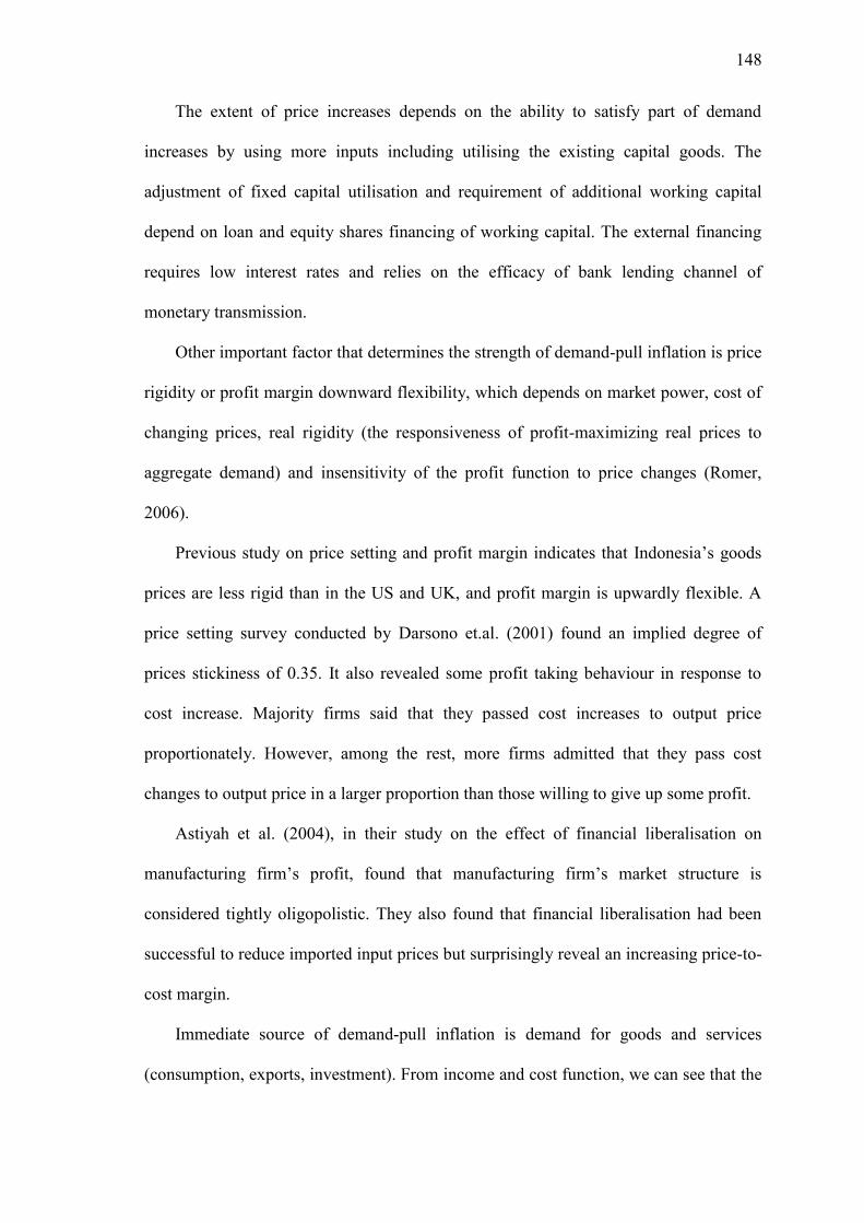
148
The extent of price increases depends on the ability to satisfy part of demand
increases by using more inputs including utilising the existing capital goods. The
adjustment of fixed capital utilisation and requirement of additional working capital
depend on loan and equity shares financing of working capital. The external financing
requires low interest rates and relies on the
efficacy of bank lending channel of
monetary transmission.
Other important factor that determines the strength of demand-pull inflation is price
rigidity or profit margin downward flexibility, which depends on market power, cost of
changing prices, real rigidity (the responsiveness of profit-maximizing real prices to
aggregate demand) and insensitivity of the profit function to price changes (Romer,
2006).
Previous study on price setting and profit margin indicates that Indonesia‘s goods
prices are less rigid than in the US and UK, and profit margin is upwardly flexible. A
price setting survey conducted by Darsono et.al. (2001) found an implied degree of
prices stickiness of 0.35. It also revealed some profit taking behaviour in response to
cost increase. Majority firms said that they passed cost increases to output price
proportionately. However, among the rest, more firms admitted that they pass cost
changes to output price in a larger proportion than those willing to give up some profit.
Astiyah et al. (2004), in their study on the effect of financial liberalisation on
manufacturing firm‘s profit, found that manufacturing firm‘s market structure is
considered tightly oligopolistic. They also found that financial liberalisation had been
successful to reduce imported input prices but surprisingly reveal an increasing price-to-
cost margin.
Immediate source of demand-pull inflation is demand for goods and services
(consumption, exports, investment). From income and cost function, we can see that the
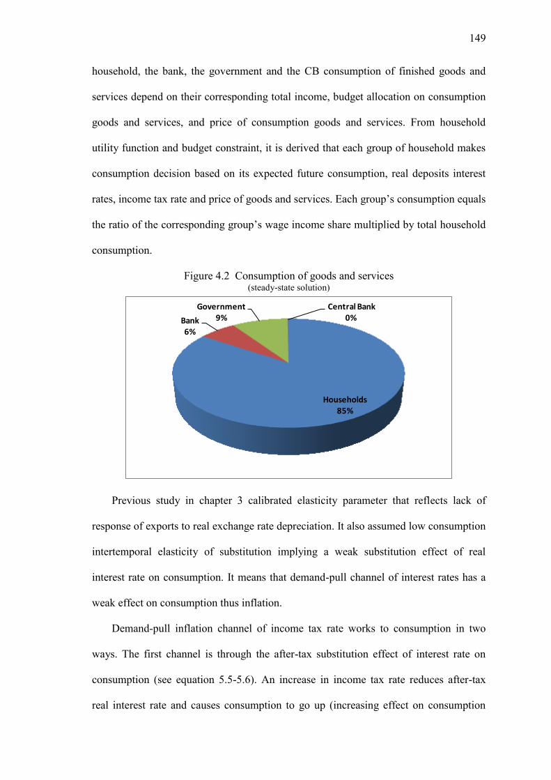
149
household, the bank, the government and the CB consumption of finished goods and
services depend on their corresponding total income, budget allocation on consumption
goods and services, and price of consumption goods and services. From household
utility function and budget constraint, it is derived that each group of household makes
consumption decision based on its expected future consumption, real deposits interest
rates, income tax rate and price of goods and services. Each group‘s consumption equals
the ratio of the corresponding group‘s wage income share multiplied by total household
consumption.
Figure 4.2 Consumption of goods and services (steady-state solution)
Households85%
Bank6%
Government9%
Central Bank0%
Previous study in chapter 3 calibrated elasticity parameter that reflects lack of
response of exports to real exchange rate depreciation. It also assumed low consumption
intertemporal elasticity of substitution implying a weak substitution effect of real
interest rate on consumption. It means that demand-pull channel of interest rates has a
weak effect on consumption thus inflation.
Demand-pull inflation channel of income tax rate works to consumption in two
ways. The first channel is through the after-tax substitution effect of interest rate on
consumption (see equation 5.5-5.6). An increase in income tax rate reduces after-tax
real interest rate and causes consumption to go up (increasing effect on consumption
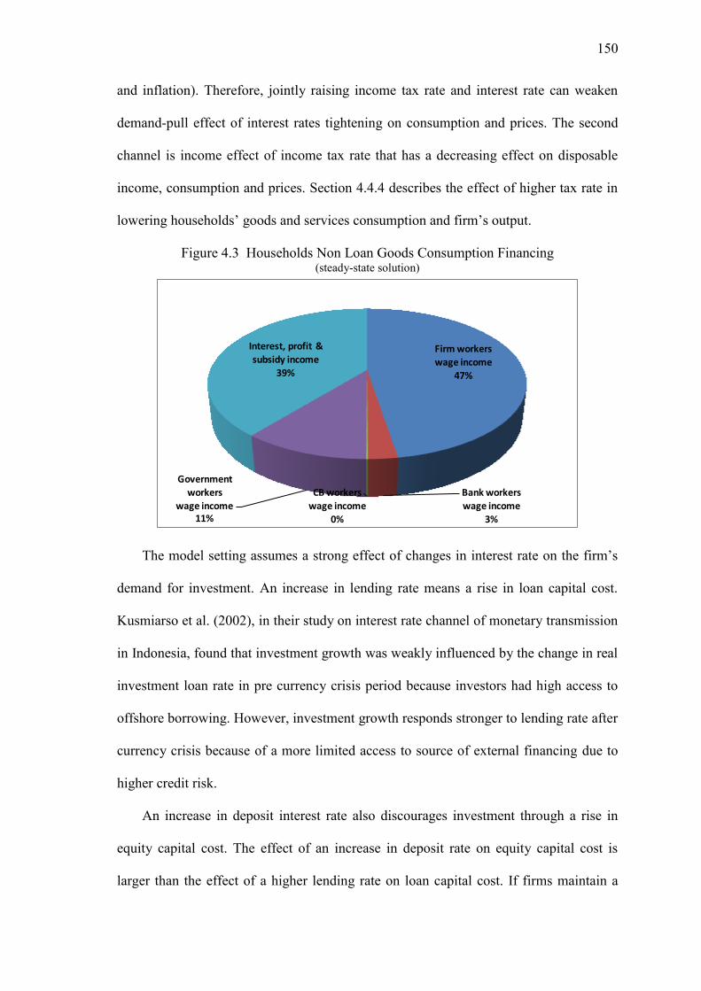
150
and inflation). Therefore, jointly raising income tax rate and interest rate can weaken
demand-pull effect of interest rates tightening on consumption and prices. The second
channel is income effect of income tax rate that has a decreasing effect on disposable
income, consumption and prices. Section 4.4.4 describes the effect of higher tax rate in
lowering households‘ goods and services consumption and firm‘s output.
Figure 4.3 Households Non Loan Goods Consumption Financing (steady-state solution)
Firm workers
wage income
47%
Bank workers
wage income3%
CB workers
wage income0%
Government workers
wage income11%
Interest, profit &
subsidy income39%
The model setting assumes a strong effect of changes in interest rate on the firm‘s
demand for investment. An increase in lending rate means a rise in loan capital cost.
Kusmiarso et al. (2002), in their study on interest rate channel of monetary transmission
in Indonesia, found that investment growth was weakly influenced by the change in real
investment loan rate in pre currency crisis period because investors had high access to
offshore borrowing. However, investment growth responds stronger to lending rate after
currency crisis because of a more limited access to source of external financing due to
higher credit risk.
An increase in deposit interest rate also discourages investment through a rise in
equity capital cost. The effect of an increase in deposit rate on equity capital cost is
larger than the effect of a higher lending rate on loan capital cost. If firms maintain a
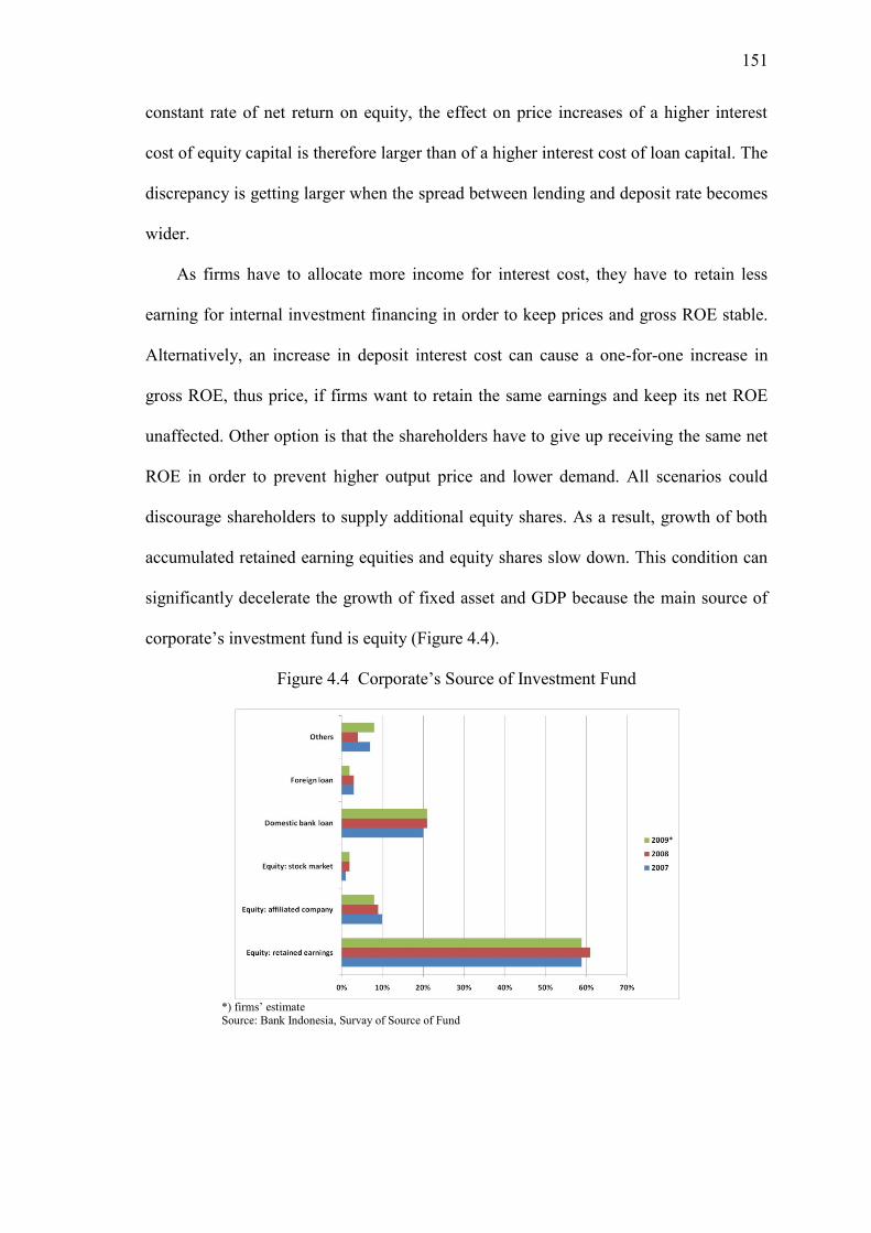
151
constant rate of net return on equity, the effect on price increases of a higher interest
cost of equity capital is therefore larger than of a higher interest cost of loan capital. The
discrepancy is getting larger when the spread between lending and deposit rate becomes
wider.
As firms have to allocate more income for interest cost, they have to retain less
earning for internal investment financing in order to keep prices and gross ROE stable.
Alternatively, an increase in deposit interest cost can cause a one-for-one increase in
gross ROE, thus price, if firms want to retain the same earnings and keep its net ROE
unaffected. Other option is that the shareholders have to give up receiving the same net
ROE in order to prevent higher output price and lower demand. All scenarios could
discourage shareholders to supply additional equity shares. As a result, growth of both
accumulated retained earning equities and equity shares slow down. This condition can
significantly decelerate the growth of fixed asset and GDP because the main source of
corporate‘s investment fund is equity (Figure 4.4).
Figure 4.4 Corporate‘s Source of Investment Fund
*) firms‘ estimate Source: Bank Indonesia, Survay of Source of Fund
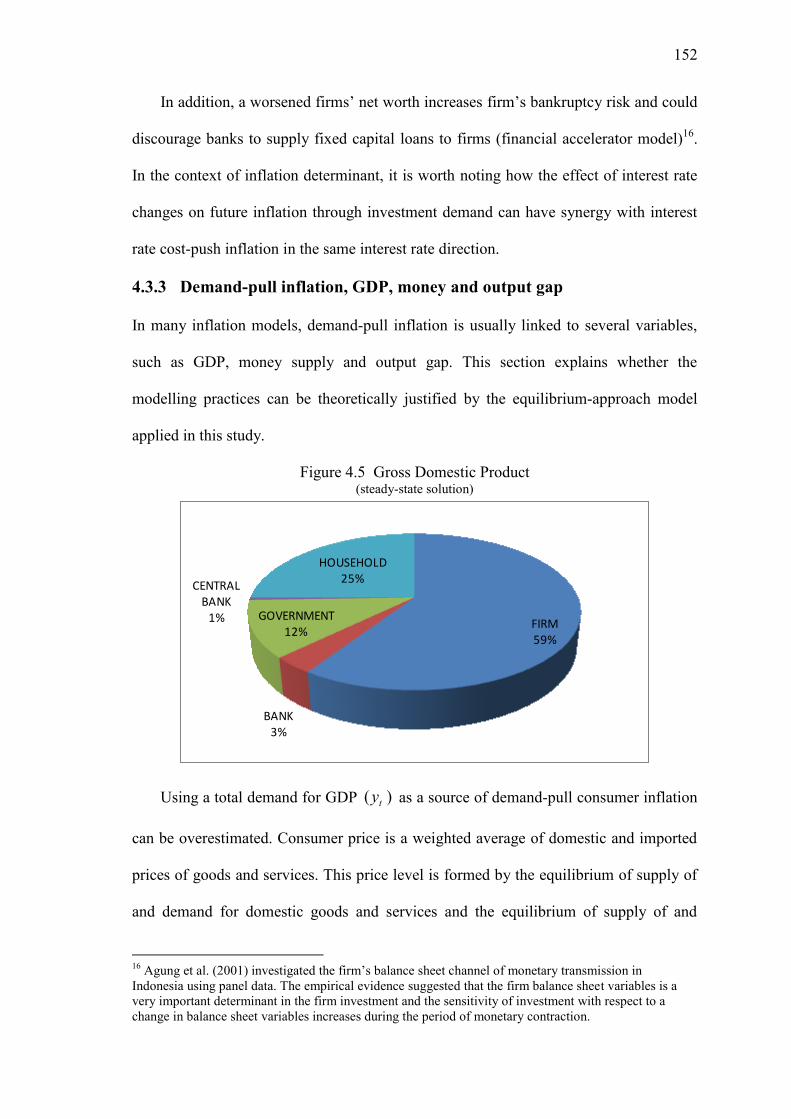
152
In addition, a worsened firms‘ net worth increases firm‘s bankruptcy risk and could
discourage banks to supply fixed capital loans to firms (financial accelerator model)16.
In the context of inflation determinant, it is worth noting how the effect of interest rate
changes on future inflation through investment demand can have synergy with interest
rate cost-push inflation in the same interest rate direction.
4.3.3 Demand-pull inflation, GDP, money and output gap
In many inflation models, demand-pull inflation is usually linked to several variables,
such as GDP, money supply and output gap. This section explains whether the
modelling practices can be theoretically justified by the equilibrium-approach model
applied in this study.
Figure 4.5 Gross Domestic Product (steady-state solution)
FIRM59%
BANK3%
GOVERNMENT12%
CENTRAL BANK
1%
HOUSEHOLD25%
Using a total demand for GDP )( ty as a source of demand-pull consumer inflation
can be overestimated. Consumer price is a weighted average of domestic and imported
prices of goods and services. This price level is formed by the equilibrium of supply of
and demand for domestic goods and services and the equilibrium of supply of and
16
Agung et al. (2001) investigated the firm‘s balance sheet channel of monetary transmission in
Indonesia using panel data. The empirical evidence suggested that the firm balance sheet variables is a
very important determinant in the firm investment and the sensitivity of investment with respect to a
change in balance sheet variables increases during the period of monetary contraction.
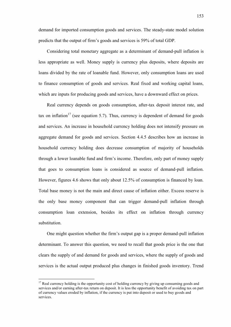
153
demand for imported consumption goods and services. The steady-state model solution
predicts that the output of firm‘s goods and services is 59% of total GDP.
Considering total monetary aggregate as a determinant of demand-pull inflation is
less appropriate as well. Money supply is currency plus deposits, where deposits are
loans divided by the rate of loanable fund. However, only consumption loans are used
to finance consumption of goods and services. Real fixed and working capital loans,
which are inputs for producing goods and services, have a downward effect on prices.
Real currency depends on goods consumption, after-tax deposit interest rate, and
tax on inflation17 (see equation 5.7). Thus, currency is dependent of demand for goods
and services. An increase in household currency holding does not intensify pressure on
aggregate demand for goods and services. Section 4.4.5 describes how an increase in
household currency holding does decrease consumption of majority of households
through a lower loanable fund and firm‘s income. Therefore, only part of money supply
that goes to consumption loans is considered as source of demand-pull inflation.
However, figures 4.6 shows that only about 12.5% of consumption is financed by loan.
Total base money is not the main and direct cause of inflation either. Excess reserve is
the only base money component that can trigger demand-pull inflation through
consumption loan extension, besides its effect on inflation through currency
substitution.
One might question whether the firm‘s output gap is a proper demand-pull inflation
determinant. To answer this question, we need to recall that goods price is the one that
clears the supply of and demand for goods and services, where the supply of goods and
services is the actual output produced plus changes in finished goods inventory. Trend
17
Real currency holding is the opportunity cost of holding currency by giving up consuming goods and
services and/or earning after-tax return on deposit. It is less the opportunity benefit of avoiding tax on part
of currency values eroded by inflation, if the currency is put into deposit or used to buy goods and
services.
154
of output or potential output does not clear goods‘ demand. The actual output does.
However, the current potential output can be an indicator for future demand-pull
inflation because it can turn to be the future actual output. A further inappropriate
inflation determinant is GDP gap, which includes output of agents other than the firm.
Another definition of output gap, which is discrepancy between actual output
produced in presumably monopolistically competitive market and output produced in
steady-state where goods market is perfectly competitive, is not applicable to stand for
demand-pull inflation determinant because price clears output supply and demand in
monopolistically competitive market.
Figure 4.6 Household Consumption
Source: Bank Indonesia
4.3.4 Bank’s interest rate and monetary and banking policy
As previously mentioned, the study in chapter 3 found that Indonesia‘s economy
characterizes lack of response of consumer price disinflation to increases in interest rate
policy, which is caused by weak demand channel and strong cost channel of interest rate
and strong cost channel and weak demand channel of exchange rate pass-through. The
finding does not mean that the central bank policy rate has a weak power on reducing
inflation. It is monetary contraction that has a weak control on combating inflation. The
155
important implication from the previous finding combined with this study is a
requirement to have a proper bank‘s deposit and lending rates to affect domestic
inflation through both demand-pull and cost-push inflation, before finally hit consumer
inflation target.
Deposit and credit rates are not only determined by the supply of and demand for
deposits and loans, but also affected by monetary and banking policy. Equation (2.6)
and (2.7) show the determinants of deposit and lending rate, which are interbank rate
targeted by CB‘s signalling policy rate, interest rate on bank reserves, inflation as a rate
of return given up for holding currency, reserve requirement policy, excess reserve
ratio, capital adequacy ratio, risk-weight of asset, operational cost and marginal profit.
Equation (2.6) highlights deposit rate setting by assuming that the bank puts all loanable
fund into interbank loans. An individual bank sets the deposit rate at a level where its
marginal revenue of holding net interbank loan and reserve account at CB equals the
sum of marginal cost of deposit, marginal cost of reserved equity capital, marginal cost
of managing deposits and marginal cost of holding currency multiplied by gross
marginal profit.
profitrginalma
b
tj
eb
tjtj
i
t
depositsmanaging
ofstcoginalmar
tj
tjt
currencyholdingof
ostcrginalma
tt
tt
equityreserveofstcoginalmar
D
tjtjt
depositsofstcoginalmar
D
tj
CBataccountreserveof
revenuerginalma
R
ttj
loannterbankinetofrevenuerginalma
ib
ttjtc
kr
D
CE
E
Ecbrierrrcbriierrrierrrcbr
b
,
1,
~
1,
,
1,
1
1~
,,3
~
,,,
)1(1~
1)(1)())(1(
(6.4)
Meanwhile, equation (2.7) shows how lending rate is set such that the net marginal
revenue of loan to the firm and household is greater or equal than that of loan to other
banks in inter bank money market.
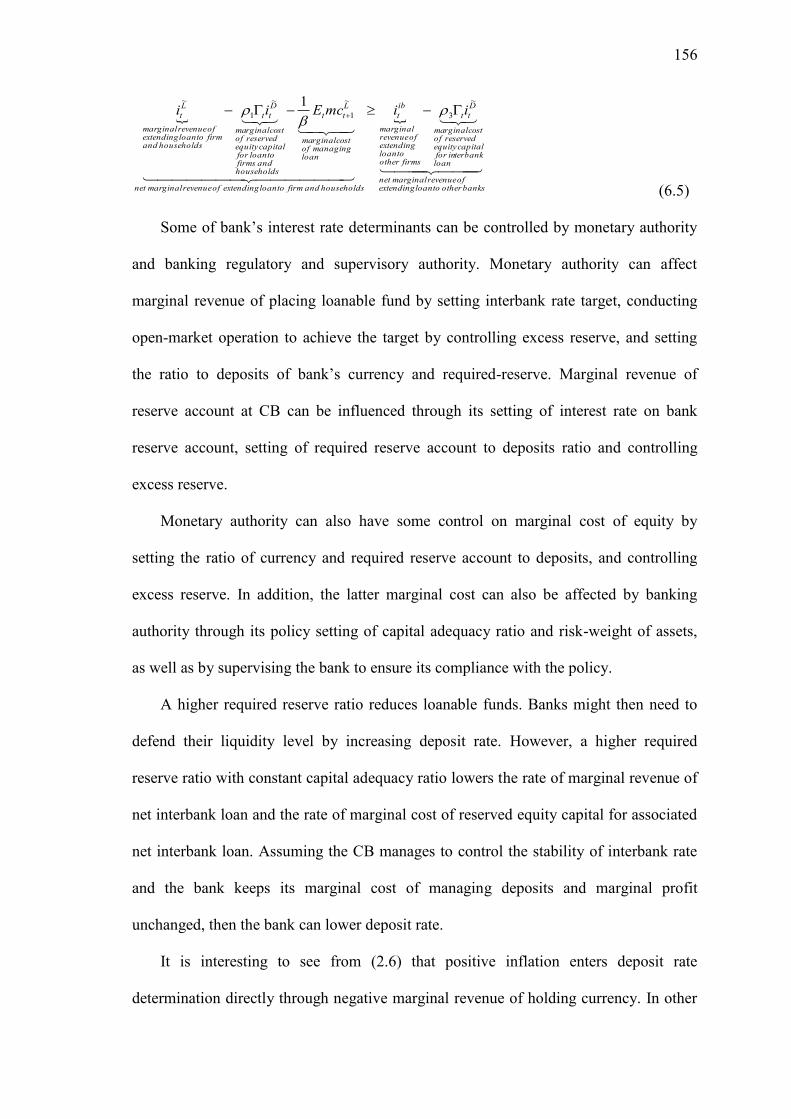
156
banksothertoloanextendingofrevenueginalmarnet
loanterbankinforcapitalequity
reservedofstcorginalma
D
tt
firmsothertoloan
extendingofrevenue
ginalmar
ib
t
householdsandfirmtoloanextendingofrevenueginalmarnet
loanmanagingof
stcorginalma
L
tt
householdsandfirms
toloanforcapitalequity
reservedofstcorginalma
D
tt
householdsandfirmtoloanextendingofrevenueginalmar
L
t iimcEii~
3
~
1
~
1
~ 1
(6.5)
Some of bank‘s interest rate determinants can be controlled by monetary authority
and banking regulatory and supervisory authority. Monetary authority can affect
marginal revenue of placing loanable fund by setting interbank rate target, conducting
open-market operation to achieve the target by controlling excess reserve, and setting
the ratio to deposits of bank‘s currency and required-reserve. Marginal revenue of
reserve account at CB can be influenced through its setting of interest rate on bank
reserve account, setting of required reserve account to deposits ratio and controlling
excess reserve.
Monetary authority can also have some control on marginal cost of equity by
setting the ratio of currency and required reserve account to deposits, and controlling
excess reserve. In addition, the latter marginal cost can also be affected by banking
authority through its policy setting of capital adequacy ratio and risk-weight of assets,
as well as by supervising the bank to ensure its compliance with the policy.
A higher required reserve ratio reduces loanable funds. Banks might then need to
defend their liquidity level by increasing deposit rate. However, a higher required
reserve ratio with constant capital adequacy ratio lowers the rate of marginal revenue of
net interbank loan and the rate of marginal cost of reserved equity capital for associated
net interbank loan. Assuming the CB manages to control the stability of interbank rate
and the bank keeps its marginal cost of managing deposits and marginal profit
unchanged, then the bank can lower deposit rate.
It is interesting to see from (2.6) that positive inflation enters deposit rate
determination directly through negative marginal revenue of holding currency. In other
157
words, inflation has a negative direct effect on deposit rate. Inflation also feeds to
deposit rate indirectly through interbank rate targeted by central bank (policy rate) to be
consistent with the achievement of inflation target. However, direction and magnitude
of indirect effect of inflation to deposit rate depends on the net effect of monetary policy
channels that drives the policy rate.
With respect to interest rate policy response to achieve consumer inflation target,
section 4.2.3 mentioned model property that does not require an ad hoc interest rate
policy rule. The free endogenous interbank rate ensures the achievement of consumer
inflation target through interaction of different monetary policy channels in several
equations such as bank‘s interest rates, consumption, investment, exchange rate, firm‘s
real marginal cost and domestic and consumer price.
As an instance, it is interesting to consider direction choice of interest rate policy
response to a more expensive import price caused by a depreciated exchange rate. With
regard to strong-direct pass-through of bank‘s interest rate to firms‘ marginal cost, we
need to lower policy rate in order to decrease domestic price. Such response could
further weaken exchange rate and increase import price, but a lesser pressure on
domestic price through interest cost channel could dampen down the effect of a higher
import price to the consumer price. It is in contrast with policy implication of exchange
rate channel by raising interest rate in response to an import price increases. In this
channel, while interest rate tightening might be able to bring exchange rate, thus import
price, back to their initial levels, interest cost channel causes domestic price to go up
hence consumer price.
One can infer the importance of having appropriate capital adequacy ratio (CAR)
from equation 6.4 and 6.5. The ratio provides a cushion that should be adequate to
absorb a reasonable amount of unexpected losses due to risks involved. Having more
158
reserved equity enables the bank to provide better protection to its depositors or other
lenders.
However, retaining more reserved equity capital corresponds to a higher marginal
cost of equity. Bank needs to place its reserved equity capital in more-liquid and less-
risky assets, which have lower return. Keeping too much reserved capital means that the
shareholders have to give up opportunity to earn more income from higher-return assets.
Alternatively, banks need to raise loan interest rate in order to protect their profit
margin. In the latter case, it implies that bank debtors pay part of excess reserve equity
capital. In the end, the cost of excess CAR is shared to the consumer of goods and
services. Thus, it would be better for banking authority to set the ceiling for capital
adequacy ratio that provides a range of optimal reserve equity capital. Section 4.4.1
shows how the bank‘s policy to have a higher capital adequacy ratio from 18% to 20%
affects the steady-state of the economy, including increasing effect on lending rates.
Having a low rate of nonperforming loans is also indirectly supportive to the
achievement of inflation target through cost channel of monetary transmission. In the
case of unrecovered bad loans, bank has to convert part of its reserved equity capital
into new assets to substitute assets loss. The bank then needs to retain more earnings to
replace the reserved equities thus keeping its capital adequacy ratio relatively stable.
This could imply a higher price of bank services when other nonfund cost and dividend
are preferably not (much) sacrificed.
Effectiveness of open market operation in achieving interbank rate target is
undoubtedly crucial in ensuring that the CB‘s policy rate is entirely passed-through to
market interbank rate, so that policy rate can play its role as a determinant of inflation.
However, further policy rate pass-through to deposit and lending rate depends on bank‘s
efficiency and profit margin flexibility, which are under limited influence of monetary
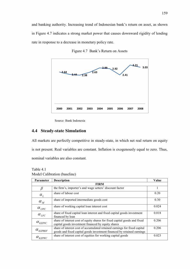
159
and banking authority. Increasing trend of Indonesian bank‘s return on asset, as shown
in Figure 4.7 indicates a strong market power that causes downward rigidity of lending
rate in response to a decrease in monetary policy rate.
Figure 4.7 Bank‘s Return on Assets
Source: Bank Indonesia
4.4 Steady-state Simulation
All markets are perfectly competitive in steady-state, in which net real return on equity
is not present. Real variables are constant. Inflation is exogenously equal to zero. Thus,
nominal variables are also constant.
Table 4.1
Model Calibration (baseline)
Parameter Description Value
FIRM
the firm‘s, importer‘s and wage setters‘ discount factor 1
L share of labour cost 0.20
M share of imported intermediate goods cost 0.30
LWC share of working capital loan interest cost 0.024
LFC share of fixed capital loan interest and fixed capital goods investment
financed by loan
0.018
KEPFC share of interest cost of equity shares for fixed capital goods and fixed
capital goods investment financed by equity shares
0.206
KEPREF share of interest cost of accumulated retained earnings for fixed capital
goods and fixed capital goods investment financed by retained earnings
0.206
KEPWC share of interest cost of equities for working capital goods 0.023
2.642.44 2.38
2.63
2.99 2.92
2.41
3.213.03
2000 2001 2002 2003 2004 2005 2006 2007 2008
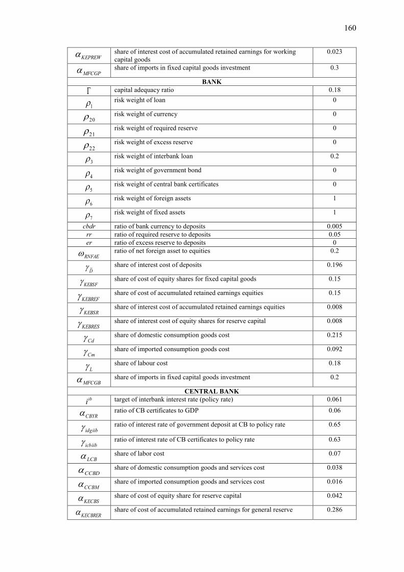
160
KEPREW share of interest cost of accumulated retained earnings for working
capital goods
0.023
MFCGP
share of imports in fixed capital goods investment 0.3
BANK
capital adequacy ratio 0.18
1 risk weight of loan 0
20 risk weight of currency 0
21 risk weight of required reserve 0
22 risk weight of excess reserve 0
3 risk weight of interbank loan 0.2
4 risk weight of government bond 0
5 risk weight of central bank certificates 0
6 risk weight of foreign assets 1
7 risk weight of fixed assets 1
cbdr ratio of bank currency to deposits 0.005
rr ratio of required reserve to deposits 0.05
er ratio of excess reserve to deposits 0
RNFAE ratio of net foreign asset to equities 0.2
D~ share of interest cost of deposits 0.196
KEBSF share of cost of equity shares for fixed capital goods 0.15
KEBREF share of cost of accumulated retained earnings equities 0.15
KEBSR share of interest cost of accumulated retained earnings equities 0.008
KEBRES share of interest cost of equity shares for reserve capital 0.008
Cd share of domestic consumption goods cost 0.215
Cm share of imported consumption goods cost 0.092
L share of labour cost 0.18
MFCGB share of imports in fixed capital goods investment 0.2
CENTRAL BANK ibi
target of interbank interest rate (policy rate) 0.061
CBYR ratio of CB certificates to GDP 0.06
idgiib
ratio of interest rate of government deposit at CB to policy rate 0.65
icbiib
ratio of interest rate of CB certificates to policy rate 0.63
LCB
share of labor cost 0.07
CCBD
share of domestic consumption goods and services cost 0.038
CCBM
share of imported consumption goods and services cost 0.016
KECBS
share of cost of equity share for reserve capital 0.042
KECBRER
share of cost of accumulated retained earnings for general reserve 0.286
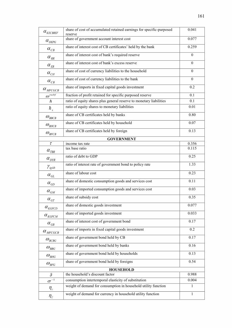
161
KECBREF
share of cost of accumulated retained earnings for specific-purposed
reserve
0.041
DEPG
share of government account interest cost 0.077
CB
share of interest cost of CB certificates‘ held by the bank 0.259
RR
share of interest cost of bank‘s required reserve 0
ER
share of interest cost of bank‘s excess reserve 0
CH
share of cost of currency liabilities to the household 0
CB
share of cost of currency liabilities to the bank 0
MFCGCB share of imports in fixed capital goods investment 0.2
recbf
fraction of profit retained for specific purposed reserve 0.1
ratio of equity shares plus general reserve to monetary liabilities 0.1
s ratio of equity shares to monetary liabilities 0.01
BBCB
share of CB certificates held by banks 0.80
BHCB
share of CB certificates held by household 0.07
BFCB
share of CB certificates held by foreign 0.13
GOVERNMENT
income tax rate 0.356
TBR
tax base ratio 0.115
DYR
ratio of debt to GDP 0.25
igiib
ratio of interest rate of government bond to policy rate 1.33
GL
share of labour cost 0.23
GD
share of domestic consumption goods and services cost 0.11
GM
share of imported consumption goods and services cost 0.03
GT
share of subsidy cost 0.35
KGFCD
share of domestic goods investment 0.077
KGFCM share of imported goods investment 0.033
GB
share of interest cost of government bond 0.17
MFCGCB share of imports in fixed capital goods investment 0.2
BCBG
share of government bond held by CB 0.17
BBG
share of government bond held by banks 0.16
BHG
share of government bond held by households 0.13
BFG
share of government bond held by foreigns 0.54
HOUSEHOLD
the household‘s discount factor 0.988
1 consumption intertemporal elasticity of substitution 0.004
c weight of demand for consumption in household utility function 1
c~ weight of demand for currency in household utility function 1
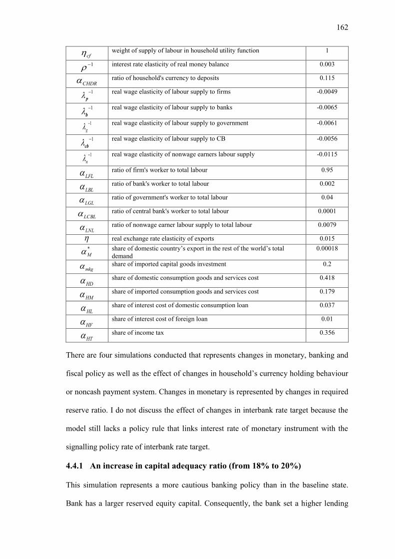
162
cf
weight of supply of labour in household utility function 1
1
interest rate elasticity of real money balance 0.003
CHDR
ratio of household's currency to deposits 0.115
1
p real wage elasticity of labour supply to firms -0.0049
1
b real wage elasticity of labour supply to banks -0.0065
1
g real wage elasticity of labour supply to government -0.0061
1
cb real wage elasticity of labour supply to CB -0.0056
1
n real wage elasticity of nonwage earners labour supply -0.0115
LFL ratio of firm's worker to total labour 0.95
LBL ratio of bank's worker to total labour 0.002
LGL ratio of government's worker to total labour 0.04
LCBL ratio of central bank's worker to total labour 0.0001
LNL ratio of nonwage earner labour supply to total labour 0.0079
real exchange rate elasticity of exports 0.015
*
M share of domestic country‘s export in the rest of the world‘s total
demand
0.00018
mkg share of imported capital goods investment 0.2
HD share of domestic consumption goods and services cost 0.418
HM share of imported consumption goods and services cost 0.179
HL
share of interest cost of domestic consumption loan 0.037
HF
share of interest cost of foreign loan 0.01
HT
share of income tax 0.356
There are four simulations conducted that represents changes in monetary, banking and
fiscal policy as well as the effect of changes in household‘s currency holding behaviour
or noncash payment system. Changes in monetary is represented by changes in required
reserve ratio. I do not discuss the effect of changes in interbank rate target because the
model still lacks a policy rule that links interest rate of monetary instrument with the
signalling policy rate of interbank rate target.
4.4.1 An increase in capital adequacy ratio (from 18% to 20%)
This simulation represents a more cautious banking policy than in the baseline state.
Bank has a larger reserved equity capital. Consequently, the bank set a higher lending
163
rate in order to maintain a zero net real return on equities. The bank supplies fewer
loans as it faces lower demand from the firm and the household.
The government obtains lower income tax revenue due to a lower firm‘s equities
and lower profit income from the central bank. With a lower goods consumptions and
investment, the government can have a lower level of debt. Thus, the bank earns lower
interest income from its government bond assets.
The CB has less income than in baseline steady-state because it has fewer net
foreign assets, which is partly due to a less currency in circulation and less bank
reserves caused by a fewer deposits. Having less income leads to a smaller liabilities
position. A lesser amount of CB balance sheet causes the bank to have a lower level of
assets in the form of CB certificates. However, the bank has a higher income because of
a higher lending rate and wider spread between lending and deposit rate.
The household has less income because of a smaller profit income from the firm‘s
return on equity and lower subsidy income. A smaller household income causes less
goods consumption. The bank also spends less on goods consumption because its goods
consumption share gets smaller as share of deposits and equities becomes larger.
Therefore, the firm faces less demand for goods output. On the supply side, although the
firm faces a less fixed capital loans, the household supply more equity capital. The
overall economy suffers from a lower level of GDP.
4.4.2 A higher required reserve ratio (from 5% to 7%)
A higher required reserve ratio is intended to represent a tighter monetary policy. As
loanable funds get smaller, banks might want to defend their liquidity level by
increasing deposit rate. However, a higher required reserve ratio reduces both marginal
revenue of net interbank loan and the rate of marginal cost of reserve equity capital.
Given a constant interbank rate controlled by monetary policy, the net effect of this
164
price channel is a lower deposit rate. This encourages households to invest more equity
on firms and banks that result in a larger production of firms‘ output and bank‘s
financial services. As firms output increases, demand for loans also goes up albeit small
increase in lending rate due to a higher marginal cost of managing loan. A higher bank
supply of financial services leads to a larger demand for deposits.
The CB has a higher interest income because its net foreign asset increases due to
expanded base money. The CB can sustain a higher steady-state financial liabilities and
net worth. Therefore, the bank gets a higher interest income from holding higher CB
certificates.
The government can obtain higher tax revenue due to a higher firm‘s and bank‘s
equity and higher CB dividend. Therefore, it can provide more subsidies, spend more on
goods consumption and investment and maintain a higher level of steady-state debt.
Thus, banks can have higher government bond‘s interest income. Overall, the economy
betters off with a higher GDP.
4.4.3 A higher tax base ratio (from 11.5% to 12%)
This simulation implies a higher income tax rate that the government has to impose. The
government has a higher income that allows it to use more consumption and investment
goods and provide more subsidies. A higher steady-state tax income also allows the
government to have a higher debt. Given the same proportion of government bonds held
by the bank, the household and the foreign, the bank earns more interest income from its
government bond assets.
Households get fewer dividends but receive much more subsidies so that the
aggregate household can earn more income. However, it has less disposable income to
spend on consumption goods. That causes a decline in the firms‘ goods and services
output.
165
A larger government income has a positive effect on the bank‘s and the CB‘s
income through their holding of government bond and fixed share of government debt
held by the bank and the CB. A higher bank income corresponds to a larger deposit fund
and further ability to extend loan. The CB can maintain a higher level of liabilities and
net worth. Although firms output declines, the other agents contribute to a large total
GDP.
4.4.4 A higher household’s currency-to-deposit ratio (from 11.5% to 13%)
This simulation represents a narrower use of noncash payment system that increases
households‘ currency holding thus reduces banks‘ loanable funds. The bank extends
fewer loans causing the firm produces fewer goods and the household has less financial
investment thus gets less revenue. Majority of households consume fewer goods and
have fewer deposits and equity assets.
The CB has larger monetary base liabilities as a resultant of a larger household
currency but smaller bank‘s currency and required reserve resulted from smaller
deposits. Thus, the CB holds more net foreign assets and has a greater income.
Subsequently, it requires a smaller CB certificates and larger net worth. Therefore, the
bank gets a fewer interest income from loans, government bonds and CB certificates.
Consequently, the government can still obtain a higher income because an increase
in central bank dividend outweighs lowered income tax revenue. This allows the
government to spend more on consumption goods and disburse more subsidies.
Accordingly, the government can have smaller debt. Thus, the household and the bank
hold fewer government bonds.
Overall, the bank produces less financial services. The smaller amount of firms and
households income outweighs the larger amount of governments and CB income,
causing the economy to produce a smaller GDP.
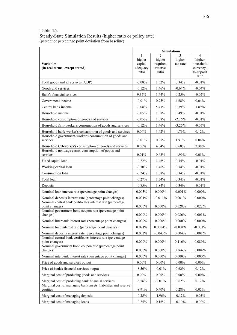
166
Table 4.2
Steady-State Simulation Results (higher ratio or policy rate) (percent or percentage point deviation from baseline)
Variables
(in real terms; except stated)
Simulations
1
higher
capital
adequacy
ratio
2
higher
required
reserve
ratio
3
higher
tax rate
4
higher
household
currency-
to-deposit
ratio
Total goods and all services (GDP) -0.08% 1.32% 0.34% -0.01%
Goods and services -0.12% 1.46% -0.64% -0.04%
Bank's financial services 9.37% 1.44% 0.25% -0.02%
Government income -0.01% 0.95% 4.68% 0.04%
Central bank income -0.08% 5.43% 0.79% 1.89%
Household income -0.05% 1.08% 0.49% -0.01%
Household consumption of goods and services -0.05% 1.08% -2.16% -0.01%
Household firm-worker's consumption of goods and services -0.12% 1.46% -3.26% -0.05%
Household bank-worker's consumption of goods and services 0.00% 1.42% -1.79% 0.12%
Household government-worker's consumption of goods and
services -0.01% 0.95% 1.91% 0.04%
Household CB-worker's consumption of goods and services 0.00% 4.04% 0.68% 2.38%
Household nonwage earner consumption of goods and
services 0.01% 0.63% -1.99% 0.01%
Fixed capital loan -0.22% 1.46% 0.34% -0.01%
Working capital loan -0.30% 1.46% 0.34% -0.01%
Consumption loan -0.24% 1.08% 0.34% -0.01%
Total loan -0.27% 1.34% 0.34% -0.01%
Deposits -0.85% 3.84% 0.34% -0.01%
Nominal loan interest rate (percentage point changes) 0.005% 0.000% -0.001% 0.000%
Nominal deposits interest rate (percentage point changes) 0.001% -0.011% 0.001% 0.000%
Nominal central bank certificates interest rate (percentage
point changes) 0.000% 0.000% 0.028% 0.022%
Nominal government bond coupon rate (percentage point
changes) 0.000% 0.000% 0.086% 0.001%
Nominal interbank interest rate (percentage point changes) 0.000% 0.000% 0.000% 0.000%
Nominal loan interest rate (percentage point changes) 0.021% 0.0004% -0.004% -0.001%
Nominal deposits interest rate (percentage point changes) 0.002% -0.043% 0.004% 0.001%
Nominal central bank certificates interest rate (percentage
point changes) 0.000% 0.000% 0.116% 0.089%
Nominal government bond coupon rate (percentage point
changes) 0.000% 0.000% 0.366% 0.004%
Nominal interbank interest rate (percentage point changes) 0.000% 0.000% 0.000% 0.000%
Price of goods and services output 0.00% 0.00% 0.00% 0.00%
Price of bank's financial services output -8.56% -0.01% 0.62% 0.12%
Marginal cost of producing goods and services 0.00% 0.00% 0.00% 0.00%
Marginal cost of producing bank financial services -8.56% -0.01% 0.62% 0.12%
Marginal cost of managing bank assets, liabilities and reserve
equities -8.91% 0.40% 0.28% 0.05%
Marginal cost of managing deposits -0.25% -1.96% -0.12% -0.03%
Marginal cost of managing loans -0.25% 0.16% -0.10% -0.02%
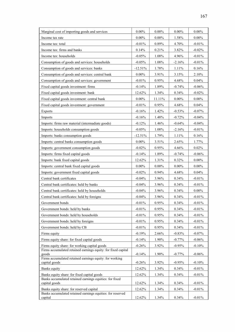
167
Marginal cost of importing goods and services 0.00% 0.00% 0.00% 0.00%
Income tax rate 0.00% 0.00% 1.58% 0.00%
Income tax: total -0.01% 0.89% 4.70% -0.01%
Income tax: firms and banks 0.14% 0.21% 3.82% -0.02%
Income tax: households -0.05% 1.08% 4.96% -0.01%
Consumption of goods and services: households -0.05% 1.08% -2.16% -0.01%
Consumption of goods and services: banks -12.51% 1.78% 1.11% 0.16%
Consumption of goods and services: central bank 0.00% 3.91% 3.15% 2.10%
Consumption of goods and services: government -0.01% 0.95% 4.68% 0.04%
Fixed capital goods investment: firms -0.14% 1.89% -0.74% -0.06%
Fixed capital goods investment: bank 12.62% 1.34% 0.34% -0.02%
Fixed capital goods investment: central bank 0.00% 11.11% 0.00% 0.00%
Fixed capital goods investment: government -0.01% 0.95% 4.68% 0.04%
Exports -0.16% 1.42% -0.53% -0.07%
Imports -0.16% 1.48% -0.72% -0.04%
Imports: firms raw material (intermadiate goods) -0.12% 1.46% -0.64% -0.04%
Imports: households consumption goods -0.05% 1.08% -2.16% -0.01%
Imports: banks consumption goods -12.51% 1.79% 1.11% 0.16%
Imports: central banks consumption goods 0.00% 3.51% 2.65% 1.77%
Imports: government consumption goods -0.02% 0.95% 4.66% 0.02%
Imports: firms fixed capital goods -0.14% 1.89% -0.74% -0.06%
Imports: bank fixed capital goods 12.62% 1.31% 0.32% 0.00%
Imports: central bank fixed capital goods 0.00% 0.00% 0.00% 0.00%
Imports: government fixed capital goods -0.02% 0.94% 4.68% 0.04%
Central bank certificates -0.04% 3.96% 0.34% -0.01%
Central bank certificates: held by banks -0.04% 3.96% 0.34% -0.01%
Central bank certificates: held by households -0.04% 3.96% 0.34% 0.00%
Central bank certificates: held by foreigns -0.04% 3.96% 0.34% -0.01%
Government bonds -0.01% 0.95% 0.34% -0.01%
Government bonds: held by banks -0.01% 0.95% 0.34% -0.01%
Government bonds: held by households -0.01% 0.95% 0.34% -0.01%
Government bonds: held by foreigns -0.01% 0.95% 0.34% -0.01%
Government bonds: held by CB -0.01% 0.95% 0.34% -0.01%
Firms equity -0.19% 2.66% -0.83% -0.07%
Firms equity share: for fixed capital goods -0.14% 1.90% -0.77% -0.06%
Firms equity share: for working capital goods -0.26% 3.92% -0.95% -0.10%
Firms accumulated retained earnings equity: for fixed capital
goods -0.14% 1.90% -0.77% -0.06%
Firms accumulated retained earnings equity: for working
capital goods -0.26% 3.92% -0.95% -0.10%
Banks equity 12.62% 1.34% 0.34% -0.01%
Banks equity share: for fixed capital goods 12.62% 1.34% 0.34% -0.01%
Banks accumulated retained earnings equities: for fixed
capital goods 12.62% 1.34% 0.34% -0.01%
Banks equity share: for reserved capital 12.62% 1.34% 0.34% -0.01%
Banks accumulated retained earnings equities: for reserved
capital 12.62% 1.34% 0.34% -0.01%
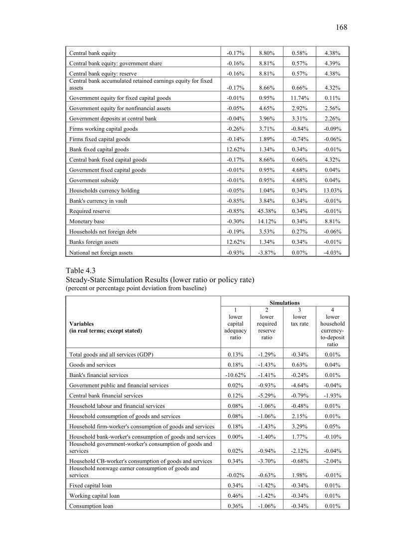
168
Central bank equity -0.17% 8.80% 0.58% 4.38%
Central bank equity: government share -0.16% 8.81% 0.57% 4.39%
Central bank equity: reserve -0.16% 8.81% 0.57% 4.38%
Central bank accumulated retained earnings equity for fixed
assets -0.17% 8.66% 0.66% 4.32%
Government equity for fixed capital goods -0.01% 0.95% 11.74% 0.11%
Government equity for nonfinancial assets -0.05% 4.65% 2.92% 2.56%
Government deposits at central bank -0.04% 3.96% 3.31% 2.26%
Firms working capital goods -0.26% 3.71% -0.84% -0.09%
Firms fixed capital goods -0.14% 1.89% -0.74% -0.06%
Bank fixed capital goods 12.62% 1.34% 0.34% -0.01%
Central bank fixed capital goods -0.17% 8.66% 0.66% 4.32%
Government fixed capital goods -0.01% 0.95% 4.68% 0.04%
Government subsidy -0.01% 0.95% 4.68% 0.04%
Households currency holding -0.05% 1.04% 0.34% 13.03%
Bank's currency in vault -0.85% 3.84% 0.34% -0.01%
Required reserve -0.85% 45.38% 0.34% -0.01%
Monetary base -0.30% 14.12% 0.34% 8.81%
Households net foreign debt -0.19% 3.53% 0.27% -0.06%
Banks foreign assets 12.62% 1.34% 0.34% -0.01%
National net foreign assets -0.93% -3.87% 0.07% -4.03%
Table 4.3
Steady-State Simulation Results (lower ratio or policy rate) (percent or percentage point deviation from baseline)
Variables
(in real terms; except stated)
Simulations
1
lower
capital
adequacy
ratio
2
lower
required
reserve
ratio
3
lower
tax rate
4
lower
household
currency-
to-deposit
ratio
Total goods and all services (GDP) 0.13% -1.29% -0.34% 0.01%
Goods and services 0.18% -1.43% 0.63% 0.04%
Bank's financial services -10.62% -1.41% -0.24% 0.01%
Government public and financial services 0.02% -0.93% -4.64% -0.04%
Central bank financial services 0.12% -5.29% -0.79% -1.93%
Household labour and financial services 0.08% -1.06% -0.48% 0.01%
Household consumption of goods and services 0.08% -1.06% 2.15% 0.01%
Household firm-worker's consumption of goods and services 0.18% -1.43% 3.29% 0.05%
Household bank-worker's consumption of goods and services 0.00% -1.40% 1.77% -0.10%
Household government-worker's consumption of goods and
services 0.02% -0.94% -2.12% -0.04%
Household CB-worker's consumption of goods and services 0.34% -3.70% -0.68% -2.04%
Household nonwage earner consumption of goods and
services -0.02% -0.63% 1.98% -0.01%
Fixed capital loan 0.34% -1.42% -0.34% 0.01%
Working capital loan 0.46% -1.42% -0.34% 0.01%
Consumption loan 0.36% -1.06% -0.34% 0.01%
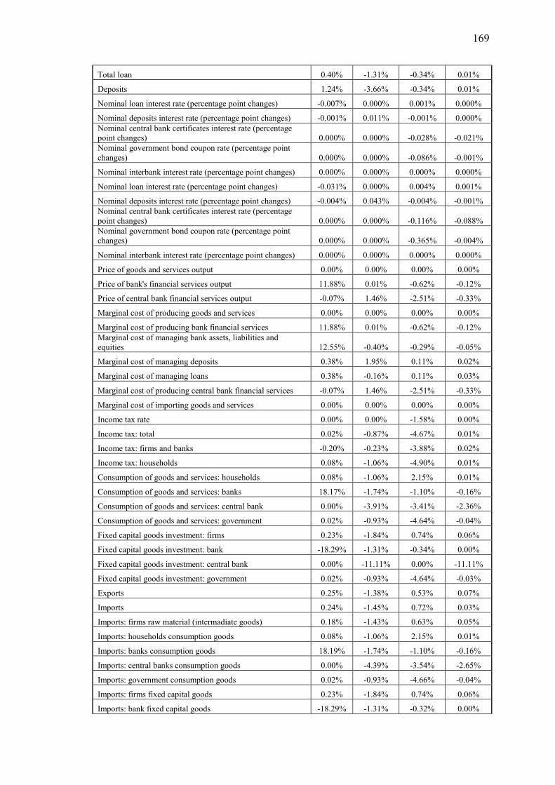
169
Total loan 0.40% -1.31% -0.34% 0.01%
Deposits 1.24% -3.66% -0.34% 0.01%
Nominal loan interest rate (percentage point changes) -0.007% 0.000% 0.001% 0.000%
Nominal deposits interest rate (percentage point changes) -0.001% 0.011% -0.001% 0.000%
Nominal central bank certificates interest rate (percentage
point changes) 0.000% 0.000% -0.028% -0.021%
Nominal government bond coupon rate (percentage point
changes) 0.000% 0.000% -0.086% -0.001%
Nominal interbank interest rate (percentage point changes) 0.000% 0.000% 0.000% 0.000%
Nominal loan interest rate (percentage point changes) -0.031% 0.000% 0.004% 0.001%
Nominal deposits interest rate (percentage point changes) -0.004% 0.043% -0.004% -0.001%
Nominal central bank certificates interest rate (percentage
point changes) 0.000% 0.000% -0.116% -0.088%
Nominal government bond coupon rate (percentage point
changes) 0.000% 0.000% -0.365% -0.004%
Nominal interbank interest rate (percentage point changes) 0.000% 0.000% 0.000% 0.000%
Price of goods and services output 0.00% 0.00% 0.00% 0.00%
Price of bank's financial services output 11.88% 0.01% -0.62% -0.12%
Price of central bank financial services output -0.07% 1.46% -2.51% -0.33%
Marginal cost of producing goods and services 0.00% 0.00% 0.00% 0.00%
Marginal cost of producing bank financial services 11.88% 0.01% -0.62% -0.12%
Marginal cost of managing bank assets, liabilities and
equities 12.55% -0.40% -0.29% -0.05%
Marginal cost of managing deposits 0.38% 1.95% 0.11% 0.02%
Marginal cost of managing loans 0.38% -0.16% 0.11% 0.03%
Marginal cost of producing central bank financial services -0.07% 1.46% -2.51% -0.33%
Marginal cost of importing goods and services 0.00% 0.00% 0.00% 0.00%
Income tax rate 0.00% 0.00% -1.58% 0.00%
Income tax: total 0.02% -0.87% -4.67% 0.01%
Income tax: firms and banks -0.20% -0.23% -3.88% 0.02%
Income tax: households 0.08% -1.06% -4.90% 0.01%
Consumption of goods and services: households 0.08% -1.06% 2.15% 0.01%
Consumption of goods and services: banks 18.17% -1.74% -1.10% -0.16%
Consumption of goods and services: central bank 0.00% -3.91% -3.41% -2.36%
Consumption of goods and services: government 0.02% -0.93% -4.64% -0.04%
Fixed capital goods investment: firms 0.23% -1.84% 0.74% 0.06%
Fixed capital goods investment: bank -18.29% -1.31% -0.34% 0.00%
Fixed capital goods investment: central bank 0.00% -11.11% 0.00% -11.11%
Fixed capital goods investment: government 0.02% -0.93% -4.64% -0.03%
Exports 0.25% -1.38% 0.53% 0.07%
Imports 0.24% -1.45% 0.72% 0.03%
Imports: firms raw material (intermadiate goods) 0.18% -1.43% 0.63% 0.05%
Imports: households consumption goods 0.08% -1.06% 2.15% 0.01%
Imports: banks consumption goods 18.19% -1.74% -1.10% -0.16%
Imports: central banks consumption goods 0.00% -4.39% -3.54% -2.65%
Imports: government consumption goods 0.02% -0.93% -4.66% -0.04%
Imports: firms fixed capital goods 0.23% -1.84% 0.74% 0.06%
Imports: bank fixed capital goods -18.29% -1.31% -0.32% 0.00%
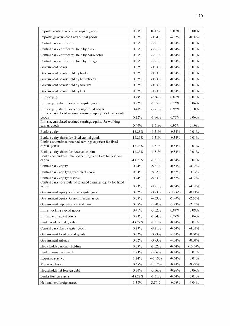
170
Imports: central bank fixed capital goods 0.00% 0.00% 0.00% 0.00%
Imports: government fixed capital goods 0.02% -0.94% -4.62% -0.02%
Central bank certificates 0.05% -3.91% -0.34% 0.01%
Central bank certificates: held by banks 0.05% -3.91% -0.34% 0.01%
Central bank certificates: held by households 0.05% -3.91% -0.34% 0.01%
Central bank certificates: held by foreign 0.05% -3.91% -0.34% 0.01%
Government bonds 0.02% -0.93% -0.34% 0.01%
Government bonds: held by banks 0.02% -0.93% -0.34% 0.01%
Government bonds: held by households 0.02% -0.93% -0.34% 0.01%
Government bonds: held by foreigns 0.02% -0.93% -0.34% 0.01%
Government bonds: held by CB 0.02% -0.93% -0.34% 0.01%
Firms equity 0.29% -2.56% 0.83% 0.07%
Firms equity share: for fixed capital goods 0.22% -1.85% 0.76% 0.06%
Firms equity share: for working capital goods 0.40% -3.71% 0.95% 0.10%
Firms accumulated retained earnings equity: for fixed capital
goods 0.22% -1.86% 0.76% 0.06%
Firms accumulated retained earnings equity: for working
capital goods 0.40% -3.71% 0.95% 0.10%
Banks equity -18.29% -1.31% -0.34% 0.01%
Banks equity share: for fixed capital goods -18.29% -1.31% -0.34% 0.01%
Banks accumulated retained earnings equities: for fixed
capital goods -18.29% -1.31% -0.34% 0.01%
Banks equity share: for reserved capital -18.29% -1.31% -0.34% 0.01%
Banks accumulated retained earnings equities: for reserved
capital -18.29% -1.31% -0.34% 0.01%
Central bank equity 0.24% -8.31% -0.58% -4.38%
Central bank equity: government share 0.24% -8.32% -0.57% -4.39%
Central bank equity: reserve 0.24% -8.33% -0.57% -4.38%
Central bank accumulated retained earnings equity for fixed
assets 0.23% -8.21% -0.64% -4.32%
Government equity for fixed capital goods 0.02% -0.93% -11.66% -0.11%
Government equity for nonfinancial assets 0.08% -4.53% -2.90% -2.56%
Government deposits at central bank 0.05% -3.90% -3.29% -2.26%
Firms working capital goods 0.41% -3.52% 0.84% 0.09%
Firms fixed capital goods 0.23% -1.84% 0.74% 0.06%
Bank fixed capital goods -18.29% -1.31% -0.34% 0.01%
Central bank fixed capital goods 0.23% -8.21% -0.64% -4.32%
Government fixed capital goods 0.02% -0.93% -4.64% -0.04%
Government subsidy 0.02% -0.93% -4.64% -0.04%
Households currency holding 0.08% -1.02% -0.34% -13.04%
Bank's currency in vault 1.23% -3.66% -0.34% 0.01%
Required reserve 1.24% -42.19% -0.34% 0.01%
Monetary base 0.45% -13.17% -0.34% -8.82%
Households net foreign debt 0.30% -3.36% -0.26% 0.06%
Banks foreign assets -18.29% -1.31% -0.34% 0.01%
National net foreign assets 1.38% 3.59% -0.06% 4.04%
171
4.5 Conclusion
The model setting and analysis presented in this paper show that the dominant, strong
effect of interest rate increases to demand-pull inflation works through investment
demand and profit margin channel. However, both channels affect inflation through
restraining supply rather than demand, causing likelihood to have a higher instead of
lower inflation. An increase in interest rate reduces demand for fixed capital investment
hence the supply of future output. It also lessens demand for and supply of working
capital through equity and loan financing that affect supply of current and future output.
Combined with robust interest rate cost-push channel and market power, this study
framework enhances the previous findings that interest rate tightening has a weak
control on reducing inflation. Monetary policy maker should bear in mind that interest
rate policy should not only be treated as a demand stabilisation but also as a cost and
supply stabilisation instrument.
It is worth noting to see that the rate of interest on depositing funds at banks serves
as a subset of rate of return on equity in all profit-maximising business units (firms and
banks). Thus, central bank‘s ability to set a proper direction and magnitude of policy
rate to achieve interbank rate target is crucial since interbank rate is the main
determinant of deposit rate. Such capability is necessary for monetary policy rate to
play its role as inflation determinant. However, we need sufficient condition to ensure
that policy rate is passed-through effectively to lending rate. Monetary and banking
authority need to promote concerted efforts to improve banks‘ operational efficiency
and dilute the viscosity of bank‘s market concentration. It is advisable that regulating
and supervising banking business competition is inherent in the task of banking
authority.

172
Furthermore, it is indispensable to realise that capital adequacy ratio is indeed an
inflation determinant as well. Thus, banking policy is necessary to support the
achievement of monetary authority‘s inflation target through setting an inflation-
oriented optimal range of capital adequacy ratio and supervising the bank‘s policy
compliance.
There is a common argument that monetary and banking policy can be conflicting
in response to banking crises. In that circumstances, monetary authority is likely to relax
its policy while banking authority is inclined to pursue a more prudent policy that may
discourage banking intermediation. This potential conflict should be able to minimise
by treating inflation as a joint overriding goal of both monetary and banking policy.
Another potential conflict of interest between the two authorities can occur when
monetary authority desires higher interest rates to fight inflation while banking authority
is concerned about the adverse effect of higher interest rate on the solvency and
profitability of banking sector (Ioannidou, 2003). However, this conflict can be weak or
even nonexistent in a certain period in the economy with weak demand channel and
strong cost channel of interest rates. The clear policy implication for such economic
environment is that the monetary authority has an opportunity to pursue disinflation by
lowering cost of capital when the state of the economy is characterized by weak demand
condition, overvalued exchange rate and favourable supply shocks. It is, therefore,
essential to enhance the linkage between monetary and banking policies making and
control.
Finally, we can further explore the findings in this study as challenging field of
research. It would be intriguing to observe the relative strength of demand-pull vs. cost-
push inflation through dynamic simulation of interest rate policy and of demand, supply
and profit margin shocks. Dynamic model can also be utilised to investigate issues

173
related to bank lending channel of monetary policy, i.e. real sector effect of changes in
bank‘s financial assets portfolio, lending and deposit rate rigidity and policy rate pass-
through to market interest rates. Empirically testing interest equity and credit cost
channel of monetary policy could also be worth justifying.
174
Appendix
Source code
$TITLE AK_PROJECT3.gms: BANKING DGE MODEL
OPTION SYSOUT=OFF;
OPTION LIMROW=50;
OPTION LIMCOL=0;
********************************
* SECTION 1 : PARAMETER VALUES *
********************************
SCALARS
*-------------------------------------------------------------------------------
* Banking parameters
*-------------------------------------------------------------------------------
CAR capital adequacy ratio /0.18/
RHO1 risk weight of placement in loan /1/
RHO20 risk weight of placement in currency /0/
RHO21 risk weight of placement in required reserve /0/
RHO22 risk weight of placement in excess reserve /0/
RHO3 risk weight of placement in interbank money market /0.20/
RHO4 risk weight of placement in government bond /0/
RHO5 risk weight of placement in central bank certificates /0/
RHO6 risk weight of placement in foreign assets /1/
RHO7 risk weight of placement in fixed assets /1/
CBDR ratio of bank currency to deposits /0.005/
RR ratio of required reserve to deposits /0.05/
ERR ratio of excess reserve to deposits /0/
LDR loan-to-deposit ratio /0.76/
LFC fixed capital loan to loan ratio /0.21/
LWC working capital loan to loan ratio /0.48/
LC consumption loan to loan ratio /0.31/
RKEBF share of equity for fixed asset /0.5/
BBFEQ ratio of bank's net foreign asset to equity /0.2/
CHG ratio of charge income to total income /0.18/
DELTAB depreciation rate of bank's fixed capital goods /0.03/
Ab technology /1/
ub capacity utilization /1/
* Cost structure
aBL share of labor cost /0.18/
*-------------------------------------------------------------------------------
* Firm parameters
*-------------------------------------------------------------------------------
A technology /1/
u capacity utilization /1/
aMf share of export in foreign economy total demand /0.000018/
ETA real exchange rate price elastity of real export /0.015/
BETHA producers's and importer's and wage setter's discount factor /1/
DELTA depreciation rate of firm's fixed capital goods /0.02/
* Cost structure
aFL share of labour /0.20/
aFRM share of imported raw material goods cost /0.30/
*-------------------------------------------------------------------------------
* Government parameters
*-------------------------------------------------------------------------------
DYR ratio of debt to GDP /0.25/
TBR tax base ratio /0.115/
DELTAG depreciation rate of govt's fixed capital goods /0.008/
RBCBG share of government bond held by CB /0.17/
RBBG share of government bond held by banks /0.16/
RBHG share of government bond held by households /0.13/
RBFG share of government bond held by foreigns /0.54/
* Cost structure
GCDYGOV share of cost of domestic consumption goods /0.11/
GCMYGOV share of cost of imported consumption goods /0.03/
WLYGOV share of employee cost /0.23/
SOYGOV share of subsidy /0.35/
aKGFCD share of cost of replacement investment: domestic /0.077/
aKGFCM share of cost of replacement investment: imported /0.033/
BGYGOV share of debt cost (solved given bg & ygov) /0.17/
*-------------------------------------------------------------------------------
* Central bank parameters
*-------------------------------------------------------------------------------
iibq interbank rate qtq /0.015/
CBYR ratio of CB certificates to GDP /0.06/
RTML ratio of CB reserve equity to monetary liabilities /0.1/
RBBCB share of CB certificates held by banks /0.80/
RBHCB share of CB certificates held by banks /0.07/
RBFCB share of CB certificates held by banks /0.13/
DELTACB depreciation rate of CB's fixed capital goods /0.001/
* Cost structure
WLYCB share of labor cost /0.07/
aDEPG share of cost of gov deposit interest /0.077/
175
BCBYCB share of interest cost of CB certificates /0.43/
CCBd share of domestic consumption goods cost /0.038/
CCBm share of imported consumption goods cost /0.016/
aKECBS share of cost of equity share for reserve capital /0.042/
aKECBRER share of cost of accumulated retained earnings for general reserve /0.286/
aKECBREF share of cost of accumulated retained earnings for specific-purposed reserve /0.041/
*-------------------------------------------------------------------------------
* Household parameters
*-------------------------------------------------------------------------------
SCALARS
SIGMA relative risk aversion (inverse of consumption intertemporal elasticity of
substitution) /265/
ETA_CONS weight of demand for consumption in household utility function /1/
ETA_CUR weight of demand for currency in household utility function /1/
ETA_L weight of supply of labour in household utility function /1/
CHDR ratio of household's currency to deposits /0.115/
RHBFH share of foreign loan interest payment in household's expenditure /0.01/
* Labour supply
RLFL ratio of firm worker to total labour /0.95/
RLBL ratio of bank worker to total labour /0.002/
RLGL ratio of government worker to total labour /0.04/
RLCBL ratio of central bank worker to total labour /0.0001/
RLNL ratio of government worker to total labour /0.0079/
* Imports share
SIMKG share of imports in firm's fixed capital goods investment /0.3/
SIMKGB share of imports in bank's fixed capital goods investment /0.2/
SIMKGG share of imports in government's fixed capital goods investment /0.2/
SIMKGCB share of imports in CB's fixed capital goods investment /0.2/
*************************************************************************************
EQUATIONS
************************************************************************************
JD.. J =E= 0;
eqG_y.. y =E= pdp*yp + pdb*yb + pdcb*ycb + ygov + yh;
*************************************************************************************
FIRM
*************************************************************************************
Output and income
eqGDPFIRM.. log(yp) =E= aFL*(log(A)+log(Lf)) + aFRM*log(cpprmm) + aFLWC*log(loanwc) +
aFLFC*log(loanfc) + aFKEPFC*log(kepfc) + aFKEPREF*log(kepref) + aFKEPREW*log(keprew) +
aFKEPWC*log(kepwc);
eqGADFIRM.. yp =E= chpd + cbpd + ccbpd + cgpd + ivpfd + ivbfd + ivgfd + ivcbfd +
x;
* Expenditure
eqL_fd.. Lf =E= aFL*pdp*yp/wf;
eqG_cpprmm.. cpprmm =E= aFRM*pdp*yp/pm;
eqG_loanwcdem.. loanwc =E= aFLWC*pdp*yp/rloanq;
eqG_loanfcdem.. loanfc =E= aFLFC*pdp*yp/(rloanq+DELTA);
eqG_aFKEP.. aFKEP =E= 1-aFL-aFRM-aFLWC-aFLFC;
eqG_aFKEPF.. aFKEPF =E= 0.9*aFKEP;
eqG_aFKEPW.. aFKEPW =E= 0.1*aFKEP;
eqG_aFKEPFC.. aFKEPFC =E= 0.5*aFKEPF;
eqG_kepfcdem.. kepfc =E= aFKEPFC*pdp*yp/(rdepq+DELTA);
eqG_aFKEPREF.. aFKEPREF =E= 0.5*aFKEPF;
eqG_keprefdem.. kepref =E= aFKEPREF*pdp*yp/(rdepq+DELTA);
eqG_aFKEPWC.. aFKEPWC =E= 0.5*aFKEPW;
eqG_kepwcdem.. kepwc =E= aFKEPWC*pdp*yp/rdepq;
eqG_aFKEPREW.. aFKEPREW =E= 0.5*aFKEPW;
eqG_keprewdem.. keprew =E= aFKEPREW*pdp*yp/rdepq;
eqG_kpfc.. kpfc =E= loanfc + kepfc + kepref;
eqG_kpwc.. kpwc =E= loanwc + kepwc + keprew;
eqG_keptot.. kep =E= kepfc + kepwc + kepref + keprew;
eqG_FDEBTOEQ.. FDEBTOEQ =E= (loanwc+loanfc)/kep;
* Equity, capital goods, investment
eqG_ivpf.. ivpf =E= DELTA*kpfc;
eqG_ivpfm.. ivpfm =E= SIMKG*ivpf;
eqG_ivpfd.. ivpfd =E= (1-SIMKG)*ivpf;
* Cost, prices, profit
eqG_pidq.. pidq =E= pitargetq;
eqG_pid.. pid =E= power((1+pidq),4)-1;
eqG_npdp.. npdp =E= p0;
eqG_pdp1.. pdp =E= npdp/p;
eqG_pdp.. pdp =E= mcp;
eqG_mcp.. log(mcp) =E= aFL*(log(wf)-log(A)-log(aFL)) + aFRM*(log(pm)-log(aFRM)) +
aFLWC*(log(rloanq)-log(aFLWC)) + aFLFC*(log(rloanq+DELTA)-log(aFLFC)) + aFKEPFC*(log(rdepq+DELTA)-
log(aFKEPFC)) + aFKEPREF*(log(rdepq+DELTA)-log(aFKEPREF)) + aFKEPWC*(log(rdepq)-log(aFKEPWC)) +
aFKEPREW*(log(rdepq)-log(aFKEPREW));
eqG_divp.. dividendfirm =E= (1-tax)*rdepq*kep;
*************************************************************************************
BANK
*************************************************************************************
Output and income
eqGDPBANK.. log(yb) =E= aBD*log(dep) + aBL*log(Lb) + aBKEBSF*log(kebsf) +
aBKEBREF*log(kebref) + aBKEBSR*log(kebsr) + aBKEBRER*log(kebrer) + aBCd*log(cbpd) + aBCm*log(cbpm);
eqGADBANK.. yb =E= (rloanq*loan + rgovq*bbg + rcbq*bbcb + rfq*q*bbf)/pdb;
eqB_ybcharge.. ybcharge =E= CHG*pdb*yb;
* Expenditure
eqEM_curb.. curb =E= CBDR*dep;
eqEM_reqres.. reqres =E= RR*dep;
176
eqEM_exres.. excesres =E= ERR*dep;
eqFIN_LDR.. dep =E= loan/LDR;
eqFIN_depcons.. dep =E= curb + reqres + excesres + loan + bbg + bbcb + bbf*q - kebrer -
kebsr;
eqFIN_depdem.. dep =E= aBD*pdb*yb/rdepq;
eqB_loanfc.. loanfc =E= LFC*loan;
eqB_loanwc.. loanwc =E= LWC*loan;
eqB_loancon.. loancon =E= LC*loan;
eqFIN_loandem.. loan =E= loancon + loanfc + loanwc;
eqEQ_kebcarrho.. keb =E= CAR*(RHO1*loan + RHO6*bbf*q + RHO7*kbfc);
eqEQ_bbf.. bbf =E= BBFEQ*keb/q;
eqB_rkbfc.. kbfc =E= RKEBF*keb;
eqB_rkebsf.. kebsf =E= 0.5*kbfc;
eqB_rkebref.. kebref =E= 0.5*kbfc;
eqG_kebsf.. kebsf =E= aBKEBSF*pdb*yb/(rdepq+DELTAB);
eqG_kebref.. kebref =E= aBKEBREF*pdb*yb/(rdepq+DELTAB);
eqG_kbfctot.. kbfc =E= kebsf+kebref;
eqB_rkebsr.. kebsr =E= 0.5*(1-RKEBF)*keb;
eqB_rkebrer.. kebrer =E= 0.5*(1-RKEBF)*keb;
eqEQ_kebsr.. kebsr =E= aBKEBSR*pdb*yb/rdepq;
eqEQ_kebrer.. kebrer =E= aBKEBRER*pdb*yb/rdepq;
eqEQ_kebdem.. keb =E= kebsr + kebrer + kbfc;
eqL_bd.. Lb =E= aBL*pdb*yb/wb;
eqG_cbpddem.. cbpd =E= aBCd*pdb*yb/pdp;
eqG_cbpmdem.. cbpm =E= aBCm*pdb*yb/pm;
eqG_cbp.. cbp =E= cbpd+cbpm;
eqB_aBCd.. aBCd =E= 0.7*(1-aBL-aBD-aBKEBSR-aBKEBRER-aBKEBSF-aBKEBREF);
eqB_aBCm.. aBCm =E= 0.3*(1-aBL-aBD-aBKEBSR-aBKEBRER-aBKEBSF-aBKEBREF);
* Equity, reserve capital, fixed capital goods, investment
eqG_ivbf.. ivbf =E= DELTAB*kbfc;
eqG_ivbfm.. ivbfm =E= SIMKGB*ivbf;
eqG_ivbfd.. ivbfd =E= (1-SIMKGB)*ivbf;
* Costs, prices, profit
eqG_pdb.. pdb =E= mcb;
eqFIN_mcb.. log(mcb) =E= aBL*(log(wb)-log(Ab)-log(aBL)) + aBCd*(log(pdp)-log(aBCd)) +
aBCm*(log(pm)-log(aBCm)) + aBKEBSF*(log(rdepq+DELTAB) - log(aBKEBSF)) + aBKEBREF*(log(rdepq+DELTAB) -
log(aBKEBREF)) + aBKEBSR*(log(rdepq)-log(aBKEBSR)) + aBKEBRER*(log(rdepq)-log(aBKEBRER)) +
aBD*(log(rdepq)-log(aBD));
eqFIN_mcbmgt.. log(mcbmgt) =E= aBL*(log(wb)-log(Ab)-log(aBL)) + aBCd*(log(pdp)-log(aBCd)) +
aBCm*(log(pm)-log(aBCm)) + aBKEBSF*(log(rdepq+DELTAB) - log(aBKEBSF)) + aBKEBREF*(log(rdepq+DELTAB) -
log(aBKEBREF));
eqFIN_mcdepm.. mcdepmgt =E= mcbmgt*aBD*yb/dep;
eqFIN_mcloanm.. mcloanmgt =E= mcdepmgt*(1/(1-(CBDR+RR+ERR)));
eqBANK_divb.. dividendbank =E= (1-tax)*rdepq*keb;
* Interest rates
eqFIN_rdep.. rdep =E= (1-S_TETA)/(S_TETA*(1-tax));
eqFIN_rdepq.. rdepq =E= sqrt(sqrt(1+rdep))-1;
eqFIN_idepq.. idepq =E= (1+rdepq)*(1+piq)-1;
eqFIN_idepqb.. idepq =E= 1/(1+(1-(CBDR+RR+ERR))*CAR*RHO3)*((1-(CBDR+RR+ERR))*iibq-
mcdepmgt);
eqFIN_iloanq.. iloanq =E= iibq+(RHO1-RHO3)*CAR*idepq+mcloanmgt;
eqFIN_rloanq.. rloanq =E= (1+iloanq)/(1+piq)-1;
*************************************************************************************
CENTRAL BANK
*************************************************************************************
Output and income
eqCB_GDP.. log(ycb) =E= WLYCB*log(Lcb) + CCBd*log(ccbpd) + CCBm*log(ccbpm) +
aKECBS*log(kecbs) + aKECBRER*log(kecbrer) + aKECBREF*log(kecbref) + BCBYCB*log(bcb) +
aDEPG*log(depg);
eqGADCB.. ycb =E= (rfq*q*bcbf + rgovq*bcbg)/pdcb;
* Expenditure
eqCB_kecbs.. kecbs =E= aKECBS*pdcb*ycb/rkecbq;
eqCB_kecbrer.. kecbrer =E= aKECBRER*pdcb*ycb/rkecbq;
eqCB_kecbref.. kecbref =E= aKECBREF*pdcb*ycb/(rkecbq+DELTACB);
eqCB_bcb.. bcb =E= BCBYCB*pdcb*ycb/rcbq;
eqCB_depg.. depg =E= aDEPG*pdcb*ycb/rdepgq;
eqL_cbd.. Lcb =E= WLYCB*pdcb*ycb/wcb;
eqCB_ccbpm.. ccbpm =E= CCBm*pdcb*ycb/pm;
eqCB_ccbpd.. ccbpd =E= CCBd*pdcb*ycb/pdp;
eqCB_ccbp.. ccbp =E= ccbpd+ccbpm;
* Equity, fixed capital goods, investment
eqCB_kecbr.. kecbr =E= RTML*(m0 + bcb + depg);
eqCB_kecbs_ras.. kecbs =E= aKECBS/(aKECBS+aKECBRER)*kecbr;
eqCB_kecbrer_ras.. kecbrer =E= aKECBRER/(aKECBS+aKECBRER)*kecbr;
eqCB_kecb.. kecb =E= kecbs + kecbrer + kecbref;
eqCB_DEPGNFA.. DEPGNFA =E= depg/(bcbf*q);
eqCB_EQNFA.. EQNFA =E= kecb/(bcbf*q);
eqCB_BCBGNFA.. BCBGNFA =E= bcbg/(bcbf*q);
eqCB_kcbfc.. kcbfc =E= kecbref;
eqCB_ivcbf.. ivcbf =E= DELTACB*kcbfc;
eqCB_ivcbfm.. ivcbfm =E= SIMKGCB*ivcbf;
eqCB_ivcbfd.. ivcbfd =E= (1-SIMKGCB)*ivcbf;
* Debt (CB certificates)
eqCB_CBYR.. bcb =E= CBYR*4*y;
eqCB_bbcbr.. bbcb =E= RBBCB*bcb;
eqCB_bhcbr.. bhcb =E= RBHCB*bcb;
eqCB_bfcbr.. bfcb =E= RBFCB*bcb/q;
* Net foreign assets
177
eqCB_bcbf.. bcbf =E= (m0 + bcb + depg + kecbs + kecbrer - bcbg)/q;
eqCB_bcbftoim.. CAD =E= bcbf*q/im;
* Monetary Base
eqEM_M0.. m0 =E= curh + curb + reqres + excesres;
* Costs, price, profit
eqG_pdcb.. pdcb =E= mccb;
eqCB_mccb.. log(mccb) =E= WLYCB*(log(wcb)-log(WLYCB)) + CCBd*(log(pdp)-log(CCBd)) +
CCBm*(log(pm)-log(CCBm)) + aKECBREF*(log(rkecbq+DELTACB)-log(aKECBREF)) + aKECBS*(log(rkecbq)-
log(aKECBS)) + aKECBRER*(log(rkecbq)-log(aKECBRER)) + BCBYCB*(log(rcbq) - log(BCBYCB)) +
aDEPG*(log(rdepgq) - log(aDEPG));
eqCB_mccbmgt.. log(mccbmgt) =E= WLYCB*(log(wcb)-log(WLYCB)) + CCBd*(log(pdp)-
log(CCBd))+CCBm*(log(pm)-log(CCBm))+aKECBREF*(log(rkecbq+DELTACB)-log(aKECBREF)) ;
eqCB_mcsbim.. mcsbimgt =E= mccbmgt*BCBYCB*ycb/bcb;
eqCB_divcb.. dividendcb =E= rkecbq*kecb;
* Interest rates
eqFIN_rresq.. rresq =E= 0;
eqFIN_isbiq.. icbq =E= SICBQ*iibq;
eqFIN_rsbiq.. rcbq =E= (1+icbq)/(1+piq)-1;
eqFIN_idepgq.. idepgq =E= 0.65*iibq;
eqFIN_rdepgq.. rdepgq =E= (1+idepgq)/(1+piq)-1;
eqFIN_ikecbq.. ikecbq =E= SIKECBQ*iibq;
eqFIN_rkecbq.. rkecbq =E= (1+ikecbq)/(1+piq)-1;
*************************************************************************************
GOVERNMENT
*************************************************************************************
Income
eqGADGOV.. ygov =E= ytax + dividendcb + rdepgq*depg;
* Tax income
eqG_tbr.. ytax =E= TBR*y;
eqG_ytax.. ytax =E= ytaxc+ytaxh;
eqG_ytaxc.. ytaxc =E= tax*rdepq*(kep + keb);
* Expenditure
eqGOV_bg.. bg =E= BGYGOV*ygov/rgovq;
eqG_kgfcd.. kgfcd =E= aKGFCD*ygov/(pdp*DELTAG);
eqG_kgfcm.. kgfcm =E= aKGFCM*ygov/(pm*DELTAG);
eqG_kgfc.. kgfc =E= kgfcd+kgfcm;
eqL_gd.. Lg =E= WLYGOV*ygov/wg;
eqG_suboil.. to =E= SOYGOV*ygov;
eqG_gmcons.. cgpm =E= GCMYGOV*ygov/pm;
eqG_gdcons.. cgpd =E= GCDYGOV*ygov/pdp;
eqG_gcons.. cgp =E= cgpd+cgpm;
* Equity, fixed capital goods, investment
eqGOV_kegrefn.. kegrefn =E= kecbs+depg;
eqG_kegref.. kegref =E= kgfc-bg;
eqGOV_ivgfd.. ivgfd =E= DELTAG*kgfcd;
eqGOV_ivgfm.. ivgfm =E= DELTAG*kgfcm;
eqGOV_ivgf.. ivgf =E= ivgfd+ivgfm;
* Debt
eqGOV_DYR.. bg =E= DYR*4*y;
eqGOV_bcbgr.. bcbg =E= RBCBG*bg;
eqGOV_bbgr.. bbg =E= RBBG*bg;
eqGOV_bhgr.. bhg =E= RBHG*bg;
eqGOV_bfgr.. bfg =E= RBFG*bg/q;
* Interest rate
eqFIN_igovq.. igovq =E= SIGOVQ*iibq;
eqFIN_rgovq.. rgovq =E= (1+igovq)/(1+piq)-1;
*************************************************************************************
HOUSEHOLD
*************************************************************************************
Income
eqGDIHOUSE.. yh =E= yhw + yhid + yhs + yhim;
* Expenditure
eqHOU_yhw.. yhw =E= wf*Lf + wb*Lb + wg*Lg + wcb*Lcb;
eqHOU_yhid.. yhid =E= dividendfirm + dividendbank - piq/(1+piq)*curh + rdepq*dep +
rgovq*bhg + rcbq*bhcb;
eqHOU_yhs.. yhs =E= to;
eqHOU_yhim.. yhim =E= (pm-q)*im;
eqHOU_ytaxh.. ytaxh =E= tax*yh;
eqHOU_loancon.. loancon =E= RHLC*yh/rloanq;
eqHOU_bfh.. bfh =E= RHBFH*yh/(rfq*q);
eqHOU_chpm.. chpm =E= RHCPM*yh/pm;
eqHOU_chpd.. chpd =E= RHCPD*yh/pdp;
eqG_chp.. chp =E= chpd+chpm;
eqHOU_RHCPD.. RHCPD =E= 0.7*(1-tax-RHLC-RHBFH);
eqHOU_RHCPM.. RHCPM =E= 0.3*(1-tax-RHLC-RHBFH);
* Labour supply
eqL_RLFL.. Lf =E= RLFL*L;
eqL_RLBL.. Lb =E= RLBL*L;
eqL_RLCBL.. Lcb =E= RLCBL*L;
eqL_RLGL.. Lg =E= RLGL*L;
eqL_RLNL.. Ln =E= RLNL*L;
eqL_L.. L =E= Lf+Lb+Lcb+Lg+Ln;
eqL_fs.. log(Lf) =E= LAMBDAF*(log(wf) + log(1-tax) - SIGMA*log(chpf) + log(ETA_CONS)
- log(ETA_L));
eqL_bs.. log(Lb) =E= LAMBDAB*(log(wb) + log(1-tax) - SIGMA*log(chpb) + log(ETA_CONS)
- log(ETA_L));
eqL_cbs.. log(Lcb) =E= LAMBDACB*(log(wcb) + log(1-tax) - SIGMA*log(chpcb) +
log(ETA_CONS) - log(ETA_L));
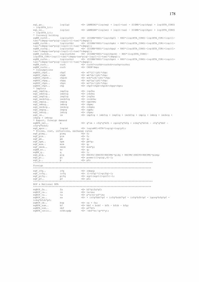
178
eqL_gs.. log(Lg) =E= LAMBDAG*(log(wg) + log(1-tax) - SIGMA*log(chpg) + log(ETA_CONS)
- log(ETA_L));
eqL_ns.. log(Ln) =E= LAMBDAN*(log(wn) + log(1-tax) - SIGMA*log(chpn) + log(ETA_CONS)
- log(ETA_L));
* Currency holding
eqEM_curhf.. log(curhf) =E= (SIGMA*RHO)*log(chpf) - RHO*(log(ETA_CONS)-log(ETA_CUR)+log((1-
tax)*idepq-tax*piq)-log(1+(1-tax)*idepq));
eqEM_curhb.. log(curhb) =E= (SIGMA*RHO)*log(chpb) - RHO*(log(ETA_CONS)-log(ETA_CUR)+log((1-
tax)*idepq-tax*piq)-log(1+(1-tax)*idepq));
eqEM_curhg.. log(curhg) =E= (SIGMA*RHO)*log(chpg) - RHO*(log(ETA_CONS)-log(ETA_CUR)+log((1-
tax)*idepq-tax*piq)-log(1+(1-tax)*idepq));
eqEM_curhcb.. log(curhcb) =E= (SIGMA*RHO)*log(chpcb) - RHO*(log(ETA_CONS)-
log(ETA_CUR)+log((1-tax)*idepq-tax*piq)-log(1+(1-tax)*idepq));
eqEM_curhn.. log(curhn) =E= (SIGMA*RHO)*log(chpn) - RHO*(log(ETA_CONS)-log(ETA_CUR)+log((1-
tax)*idepq-tax*piq)-log(1+(1-tax)*idepq));
eqEM_curh.. curh =E= curhf+curhb+curhcb+curhg+curhn;
eqEM_curhr.. curh =E= CHDR*dep;
* Consumptions
eqHOU_chpf.. chpf =E= wf*Lf/(yh)*chp;
eqHOU_chpb.. chpb =E= wb*Lb/(yh)*chp;
eqHOU_chpcb.. chpcb =E= wcb*Lcb/(yh)*chp;
eqHOU_chpg.. chpg =E= wg*Lg/(yh)*chp;
eqHOU_chpn.. chpn =E= wn*Ln/(yh)*chp;
eqHOU_chpt.. chp =E= chpf+chpb+chpcb+chpg+chpn;
* Imports
eqG_impfcg.. impfcg =E= ivpfm;
eqG_imbfcg.. imbfcg =E= ivbfm;
eqG_imgfcg.. imgfcg =E= ivgfm;
eqG_imcbfcg.. imcbfcg =E= ivcbfm;
eqG_impig.. impig =E= cpprmm;
eqG_imbcg.. imbcg =E= cbpm;
eqG_imcbcg.. imcbcg =E= ccbpm;
eqG_imgcg.. imgcg =E= cgpm;
eqG_imhcg.. imhcg =E= chpm;
eqG_im.. im =E= impfcg + imbfcg + imgfcg + imcbfcg + impig + imbcg + imcbcg +
imgcg + imhcg;
* Export, foreign demand
eqNFA_net.. x =E= q*im + rfq*q*bfh + rgovq*q*bfg + rcbq*q*bfcb - rfq*q*bbf -
rfq*q*bcbf;
eqG_xpor.. log(x) =E= log(aMf)+ETA*log(q)+log(yf);
* Prices, cost, inflations, exchange rates
eqF_pimq.. pimq =E= 0;
eqF_pim.. pim =E= 0;
eqF_pm.. pm =E= q;
eqF_npm.. npm =E= pm*p;
eqF_mcm.. mcm =E= q;
eqF_nmcm.. nmcm =E= mcm*p;
eqEM_er.. er =E= q;
eqEM_q.. q =E= 1;
eqG_piq.. piq =E= RHCPD/(RHCPD+RHCPM)*pidq + RHCPM/(RHCPD+RHCPM)*pimq;
eqG_pi.. pi =E= power((1+piq),4)-1;
eqG_p.. p =E= p0;
*************************************************************************************
Foreign
************************************************************************************
eqF_rfq.. rfq =E= rdepq;
eqF_irfq.. irfq =E= (1+rfq)*(1+pifq)-1;
eqF_pifq.. pifq =E= sqrt(sqrt(1+pif))-1;
eqF_pf.. pf =E= p0;
*************************************************************************************
BOP & National NFA
************************************************************************************
eqBOP_fa.. fa =E= bf*pifq*pf;
eqBOP_ca.. ca =E= ta+sa;
eqBOP_ta.. ta =E= p*x/er-pf*im;
eqBOP_sa.. sa =E= + irfq*bbf*pf + irfq*bcbf*pf - irfq*bfh*pf - igovq*bfg*pf -
icbq*bfcb*pf;
eqBOP_ob.. bop =E= ca + fa;
eqNFA_sum.. bf =E= bbf + bcbf - bfh - bfcb - bfg;
eqNFA_nom.. nbf =E= pf*bf;
eqNFA_ratio.. nfdtogdp =E= -nbf*er/(p*4*y);

Chapter 5
Concluding remarks
180
This thesis has attempted to produce contribution to some macroeconomic issues related
to monetary policy, monetary transmission and inflation, using dynamic and steady-
state general equilibrium models. Issues covered in this framework of central bank core
function are:
1. Optimal monetary policy response and policy interest rate pass-through to market
interest rates
2. Relations between interest rate policy and monetary aggregate
3. Exchange rate pass-through, transient exchange rate depreciation and moderate
currency crises
4. Relative strength of monetary transmission to inflation through demand, supply and
cost channel
5. Cost-push vs. demand-pull inflation
6. Role of banking in monetary transmission to inflation through financial intermediary
and the setting of deposit and lending rate
7. Nexus between monetary and banking policy
The interest cost of equity and borrowing is central to the framework of this study.
It is instigated by the central bank‘s policy rate and transmitted through banking
intermediary function to the interest rate cost-push inflation. Assuming that deposit rate
is the lower bound of goods-producers‘ rate of return on equity, then we can say that the
interest rate is a large contributor to price determination. It is in line with the estimated
low positive intertemporal elasticity of consumption and the role of return on equity as
the largest contributor for Indonesia‘s gross domestic income. Moreover, it is consistent
with the model estimate of low firm‘s wage and negative real wage elasticity of labour
supply, which both indicated a wide income gap.
181
This role of interest rate cost on inflation has significant implication on the
magnitude of policy response. In the case of moderate currency crisis in the second
essay, the finding shows that the proper monetary policy response is the smallest
interest rate increases within the feasible set of monetary policy responses provided by
the model. As the implication of strong interest rate cost channel of monetary
transmission, the second essay also discusses the requirement of long-term policies
complement such as improvement in economic structure. They are expected to
strengthen monetary policy in its role as demand stabilisation instrument through
lessening the power of interest rate cost channel.
The third essay focuses on how monetary policy should play its function as the
short-run demand, supply and cost stabilisation instrument. However, policy focus in
those two essays shares the same required policy supplement. It is a longer-term and
less-immediate complementary policy solution to monetary policy: boosting
competition in goods and financial market.
The third essay also underlined a key concept that the main positive determinant of
deposit rate is the central bank‘s policy rate, not inflation. Inflation feeds to deposit rate
indirectly through policy rate that is set consistent with the achievement of the inflation
target. The direction and magnitude of the indirect effect of inflation to deposit rate
depend on the net effect of monetary policy channels that drive the policy rate response.
In finding answers to the main issues related to monetary policy, monetary
transmission and inflation, this study built a modelling framework that features
Indonesia‘s distinctive agent‘s behaviour and the structure and market imperfection of
Indonesia‘s economy. The features distinguish them with those of advanced economies.
In terms of their comparison to those in an advanced economy, the features comprise (a)
a less rigid domestic and import prices, (b) much lower intertemporal elasticity of

182
consumption and (c) much smaller interest rate elasticity of real money balance, which
is associated with higher household currency-to-deposit ratio. Other distinct economic
features include the structure of agent‘s expenditure and income.
With respect to price rigidity, the assumption of a more flexible domestic price than
that in advanced economies resulted in a coefficient of contemporaneous real marginal
cost in the new Keynesian Phillip curve that is higher than that of expected inflation. It
means that inflation depends more on the current pressure on the price-to-cost margin
than on the expected future profit margin. It implies that the weight for the expectation
of changes in the contemporaneous inflation determinant is larger than that for the
expectation of future inflation determinant. That makes a distinction with the researches
on advanced economies that assumed that prices are quite rigid, which is more rigid
than what I assumed for Indonesia‘s economy. In this case, inflation depends more on
the expected future profit margin than on the current pressure on the price-to-cost
margin.
However, the assumption of less rigid price in Indonesia than in advanced
economies might be inappropriate for downward price rigidity if the model
accommodates asymmetric rigidity feature. We could have a hypothesis that prices are
stickier downward in Indonesia than in advanced economies because firms in the former
economy has a lower degree of competition than those in the later.
With regard to the behaviour of household, the third part of this study managed to
introduce heterogeneous households, in which the household is separated into wage-
and nonwage-earners. I classified the former into four groups according to the agents
where they supply their labour services. I also found and discussed negative labour
supply elasticity with respect to changes in real wage. The third model also produces
four groups of individual real wages, with the real wage of firm‘s workers is much
183
smaller than those of other workers and the individual real income of nonwage-earners.
That implies a high degree of income inequality, which is a common macroeconomic
feature in developing economies.
With respect to interest rate cost channel, I applied the essential assumption
mentioned earlier that the deposit rate serves as the lower bound of the rate of return on
equity for all profit-seeking agents. Therefore, the interest cost channel of monetary
policy consist not only cost of real loan but also cost of real equity.
Meanwhile, the assumption in this study makes a distinction with several studies
(see, for instance, Christiano and Eichenbaum 1992), in which the justification for
interest rate cost channel is through interest cost of working capital loans because firms
need financing for purchasing raw material and paying the employee‘s salary prior to
the sale of the product. The inclusion of cost of equity in the interest cost channel for
this study relies on two implied assumptions. First, that the firm‘s loan-to-equity ratio in
Indonesia‘s nonfinancial business units is lower than that in developed economies.
Second, that the firm‘s market power in the former economy is stronger than in the
later, causing likelihood to have the rate of return on equity greater than deposit rate in
most of the time. It is in line with the view of Chowdhury et al. (2006) that the logic of
interest rate effects on firms‘ costs also applies when firms are primarily financed by
internal funds.
With respect to linking financial intermediary to the real sector, central bank and
government, this study has introduced the interpretation of real equity, real loan, real
deposits, real government bonds and real CB certificates as a key idea for linking those
sectors. The model features the demand for and supply of financial intermediation
services, which, combined with other agent‘s output or income, form the total of GDP.
This approach makes dissimilarity with common macroeconomic modelling methods,

184
which assume that GDP is represented by the firm‘s output. Since GDP is aggregated
into agents‘ output or income and there are five groups of household-labour suppliers,
then we can have five groups of household-consumers. This feature enriches the
monetary transmission mechanism to total consumption, GDP and inflation.
Furthermore, the third essay has a feature that all agents have own budget and
balance-sheet constraints and objective function, where all balance-sheet and budget
equation are linked and consolidated. These modelling characteristics bring
consequence that the government does not need a common ad-hoc tax rule i.e the one
that maintains a fixed ratio of primary fiscal deficit-to-GDP, because tax variable works
as an automatic adjustment in ensuring the government budget balanced. With regard to
tax, this study could be able to provide a better representation of Indonesia‘s economic
environment as a developing economy if the model also incorporates tax on
consumption and relaxes the implicit assumption of zero tax avoidance.
In addition to the aforementioned properties of balance sheet, budget constraint and
objective function, the modelling of deposit and lending rates determination rules out
the need to have an ad-hoc interest rate policy rule of targeting interbank rate to achieve
consumer inflation target. It also allows the model to present the banking institution that
has two market interest rates that can move in disharmony with policy rate. Yet the third
model still lacks a behavioural equation that serves as a rule for the interest rate of
monetary instrument. Moreover, it is also deficient in the behavioural equation of
government bond interest rate. However, the overall modelling approach managed to
minimise the involvement of non micro-founded behavioural equation in general
equilibrium model.
185
References
Agénor, Pierre-Richard and Peter J. Montiel (2008). Development Macroeconomics,
Third Edition. Princeton University Press.
Agung, J., Rita Morena, Bambang Pramono, Nugroho J. Prastowo (2001). ―Bank
Lending Channel of Monetary Transmission in Indonesia‖, Bank Indonesia
Working Paper.
Agung, J., Rita Morena, Bambang Pramono, Nugroho J. Prastowo (2001). ―Monetary
Policy and Firm Investment: Evidence for Balance Sheet Channel in Indonesia‖,
Bank Indonesia Working Paper.
Al-Eyd, Ali and Stephen G. Hall (2006). ―Financial Crisis, Effective Policy Rules and
Bounded Rationality in a New keynesian Framework‖. NIESR Discussion Paper
No. 272.
Altissimo, Filippo, Michael Ehrmann, Frank Smets (2006). ―Inflation Persistence and
Price-setting Behaviour in The Euro Area: A Summary of The IPN Evidence‖.
National Bank of Belgium Working Paper.
Ambler, Steve, Ali Dib, and Nooman Rebei (2003). ―Nominal Rigidities and Exchange
Rate Pass-Through in a Structural Model of a Small Open Economy‖. Bank of
Canada Working Paper 2003-29.
Ascari, Guido (2003). ―Staggered prices and trend inflation: some nuisances‖. Bank of
Finland Discussion Papers 27.
Aoki, Kosuke (2001). ―Optimal monetary policy responses to relative-price changes‖,
Journal of Monetary Economics 48 (2001), pp. 55-80.
Atta-Mensah, Joseph and Ali Dib (2008). Bank lending, credit shocks, and the
transmission of Canadian monetary policy, International Review of Economics
and Finance, Volume 17, Issue 1, 2008, Pages 159-176.
Azis, Iwan J. (2008). ―Indonesia‘s Slow Recovery After Meltdown‖, Asian Economic
Papers 7:1, The Earth Institute at Columbia University and the Massachusetts
Institute of Technology.
Bagliano, Fabio-Cesare & Giuseppe Bertola (2007). Models for Dynamic
Macroeconomics. Oxford University Press.
Bailliu, Jeannine, Daniel Garces, Mark Kruger and Miguel Messmacher (2002).
―Explaining and Forecasting Inflation in Emerging Markets: the Case of
Mexico‖, Bank of Canada Working Paper 2003-17.
Bank Indonesia (2010). Indonesia‘s Economic Report, April.
Bank Indonesia (2009). Financial Report 2008, May.
Barth, M.J., Ramey, V. (2001). ―The Cost Channel of Monetary Transmission‖. NBER
Macroeconomic Annual, pp. 199–239.
Besar, Dwityapoetra S. and Alistair Milne (2009). ―Competition in Indonesian
Provincial Banking Markets: A Comparison of Structural and New Empirical
Industrial Organization Models‖. Working Paper, Cass Business School, City
University London.
186
Blanchard, Olivier J. & Nobuhiro Kiyotaki (1999). ―Monopolistic Competition and the
Effects of Aggregate Demand‖. American Economic Review, Vol. 77, No. 4,
647-666.
Blanchard, Olivier J. & Stanley Fisher (1989). ―Lectures on Macroeconomics‖. The
MIT Press.
Blinder, Alan S. (1991). ―Why are prices Sticky? Preliminary Results from an Interview
Study‖, American Economic Review Vol. 81(2), pp. 89-100.
Blinder, Alan S. (2010). ―How Central Should the Central Bank Be?‖, CEPS Working
Paper, No. 198.
Calvo, Guillermo (1983). ―Staggered Proces in A Utility-Maximizing Framework‖,
Journal of Monetary Economics 12 (1983), pp. 383-398.
Calvo, Guillermo and Reinhart C.M. (2002). ―Fear of Floating‖, Quarterly Journal of
Economics, Vol.117(2), pp. 379-408.
Camilo E. Tovar (2008). ―DSGE models and central banks‖. Bank for International
Settlements Working Papers No 258.
Campa, J. and L. Goldberg (2001). ―Exchange Rate Pass-Through into Import Prices: A
Macro and Micro Phenomenon." Federal Reserve Bank of New York.
Castelnuovo, Efrem and Paolo Surico (2006). ―The price puzzle: fact or artifact?‖ Bank
of England Working Paper No. 288.
Cecchetti, Stephen (2001). ―Making Monetary Policy: Objectives and Rules‖.
Misconceptions Regarding Rules vs. Discretion for Monetary Policy‖. Oxford
Review of Economic Policy Vol.16.
Cecchetti, Stephen G., Piti Disyatat and Marion Kohler (2009). ―Integrating financial
stability: new models for a new challenge‖. An essay for the joint BIS-ECB
Workshop on "Monetary policy and financial stability", Basel, Switzerland, 10-
11 September 2009.
Chowdhury, A., Roger Ham (2009). ―Inflation Targeting in Indonesia: Searching for a
Threshold‖. The Singapore Economic Review Vol.54, Issue 04, pp. 645-655.
Chowdhury, A., Hermanto Siregar (2004). ―Indonesia‘s Monetary Policy Dilemma –
Constraints of Inflation Targeting‖. The Journal of Developing Areas, Volume
37, Number 2, Spring 2004, pp.137-153.
Chowdhury, Ibrahim, Mathias Hoffmanna, and Andreas Schabert (2006). ―Inflation
dynamics and the cost channel of monetary transmission‖. European Economic
Review 50, pp. 995–1016.
Christiano, Lawrence J. and Martin Eichenbaum (1992). ―Liquidity Effects and the
Monetary Transmission Mechanism‖. American Economic Review, Vol.82, 346-
53.
Christiano, Lawrence J., Christopher Gust and Jorge Roldos (2004). ―Monetary policy
in a financial crisis‖ Journal of Economic Theory, Vol. 119, pp. 64-103.
Christiano, Lawrence J., Martin Eichenbaum, and Charles L. Evans (2005). ―Nominal
Rigidities and the Effects of a Shock to Monetary Policy,‖ Journal of Political
Economy, Vol. 113(1), 1−45.
187
Clarida, R., J. Gali, M. Gertler (1999). ―The Science of Monetary Policy: A New
Keynesian Perspective‖. Journal of Economic Literature, Vol. 37, Issue 4, 1661-
1707.
Copeland, Laurence (2005). ―Exchange Rates and International Finance‖. Prentice Hall.
Cúrdia, Vasco and Michael Woodford (2008). ―Credit Frictions and Optimal Monetary
Policy‖. Department of Economics, Columbia University, Discussion Paper No.
0809-02.
D‘Adda, C. and Antonello E. Scorcu (2003). ―On the stability of the output-capital
ratio‖. Economic Modelling, vol. 20(6), pages 1175-1189.
Darsono, Akhis R. Hutabarat, Diah Esti Handayani, Hery Indratno, Retno Muhardini
(2002). ―Survey of Bussiness Price Setting Behavior‖. Paper presented at The
26th
CIRET Conference, Taipei, October 2002.
deBrouwer, Gordon and Neil R. Ericsson (1998). Modeling Inflation in Australia.
Journal of Business & Economic Statistics, Vol. 16, No. 4, 433-449.
Devereux, Michael B., Philip R. Lane and Juanyi Xu (2006). ―Exchange Rates and
Monetary Policy in Emerging Market Economies‖. The Economic Journal, 116
(April), 478–506. Royal Economic Society 2006.
Devereux, Michael B. and Yetman, James (2005). ―Price Adjustment and Exchange
Rate Pass-through‖. Available at SSRN: http://ssrn.com/abstract=779846
Devereux, M. and J. Yetman. 2003. ―Price Setting and Exchange Rate Pass-Through:
Theory and Evidence." In Price Adjustment and Monetary Policy. Proceedings
of a conference held by the Bank of Canada, November 2002.
Devereux, M. 2001. ―Monetary Policy, Exchange Rate Flexibility and Exchange Rate
Pass-Through." In Revisiting the Case for Flexible Exchange Rates, 47-82.
Proceedings of a conference held by the Bank of Canada, November 2000.
Ottawa: Bank of Canada.
DiCecio, Riccardo and Edward Nelson (2007). ―An Estimated DSGE Model for the
United Kingdom‖. Federal Reserve Bank of St.Louis, Working Paper 2007-
006A
Dossche, Maarten (2009). ―Understanding inflation dynamics: Where do we stand?‖
National Bank of Belgium Working Paper Research No.165.
Driskill, Robert A. and Steven M. Sheffrin (1985). ―The "Patman Effect" and
Stabilization Policy‖. The Quarterly Journal of Economics, Vol. 100, No. 1
(Feb., 1985), pp. 149-163. The MIT Press.
Drud, Arne (2006). ―CONOPT‖, GAMS – The Solver Manuals, ARKI Consulting and
Development A/S, Bagsvaerd, Denmark.
Edward, Sebastian (1986). ―Are Devaluations Contractionary?‖, The Review of
Economics and Statistics, Vol. 68, No.3 (Aug., 1986), pp. 501-508.
Ehrenberg, Ronald G. & Robert S. Smith (2009). Modern Labor Economics – Theory
and Public Policy, Tenth Edition. Pearson Education, Inc.
Eichenbaum, M. (1992). ―Comment on ‗Interpreting the macroeconomic time series
facts: the effects of monetary policy‘ by C.A. Sims‖. European Economic
Review, 36, pp. 1001–1011.

188
Erceg, Christopher J., Andrew T. Levin (1983). ―Imperfect credibility and inflation
persistence‖, Journal of Monetary Economics 50 (2003), pp. 915-955.
Freixas, Xavier and Jean-Charles Rochet (2008). Microeconomics of Banking. The
MIT Press.
Fuhrer, Jeffrey C. (2006). ―Intrinsic and Inherited Inflation Persistence‖. International
Journal of Central Banking.
Gali, Jordi, Mark Gertler (1999). ―Inflation dynamics: A Structural econometric
analysis‖. Journal of Monetary Economics, Vol. 44, 195-222.
Gali, Jordi, Tommaso Monacelli (1999). ―Monetary Policy and Exchange Rate
Volatility In Small Open Economy‖. NBER Working Paper 8905.
Garratt, Anthony, Kevin Lee, M. Hashem Pesaran, Yongcheol Shin (2006). ―Global and
National Macroeconometric Modelling – A Long-Run Structural Approach,
Draft Chapter 1-3.
Gerali, Andrea, Stefano Neri, Luca Sessa, and Federico M. Signoretti (2010). ―Credit
and Banking in a DSGE Model of the euro area‖. Banca d‘Italia Working Paper
Gibson, Alfred Herbert (1923). ―The future course of high class investment values‖.
Banker‘s Magazine, January, pp. 15–34.
Goodfriend, Marvin & Bennett T. McCallum (2007). "Banking and Interest Rates in
Monetary Policy Analysis: A Quantitative Exploration," NBER Working
Papers 13207, National Bureau of Economic Research, Inc.
Hamann, Franz (2004). ―On the Use of Models for Monetary Policy in Colombia: a
Technocrat‘s Perspective‖. Webpondo.org edition No.13, July-Sep 2004.
Hall, Simon, Mark Walsh, Anthony Yates (1997). ―How do UK companies set prices?‖.
Bank of England Working Paper 8905.
Harrison, Richard, Kalin Nikolov, Meghan Quinn, Gareth Ramsay, Alasdair Scott and
Ryland Thomas (2005). ―The Bank of England Quarterly Model‖. Bank of
England.
Henzel, Steffen, Oliver Hülsewig, Eric Mayer, Timo Wollmershäuser (2008). ―The
price puzzle revisited: Can the cost channel explain a rise in inflation after a
monetary policy shock?‖
Hossain, A (2006). ―Sources of Economic Growth in Indonesia, 1966-2003‖ Journal of
Applied Econometrics and International Development, Vol.6 Issue 2.
Husman, Jardine A. (2005). ―Pengaruh Nilai Tukar Riil Terhadap Neraca Perdagangan
Bilateral Indonesia: Kondisi Marshall-Lerner dan Fenomena J-Curve (The
Effect of Real Exchange Rate on Indonesia‘s Bilateral Trade Balance: Marshall-
Lerner Condition and J-Curve Phenomenon)‖. Buletin Ekonomi Moneter dan
Perbankan Bank Indonesia (Volume 8 No.3).
Ioannidou, Vasso P. (2005). ―Does monetary policy affect the central bank‘s role in
banking supervision?‖, Journal of Financial Intermediation 14 (2005) 58–85.
Kamihigashi, Takashi (2008). "Transversality conditions and dynamic economic
behaviour." The New Palgrave Dictionary of Economics. Second Edition. Eds.
Stephen N. Durlauf and Lawrence E. Blume. Palgrave Macmillan, 2008. The
189
New Palgrave Dictionary of Economics Online. Palgrave Macmillan. 21 June
2010 <http://www.dictionaryofeconomics.com/article?id=pde2008_T000217>
Kendrick, David A., P. Ruben Mercado, and Hans M. Amman (2005). ‖Computational
Economics‖. Princeton University Press.
Knoop, Todd A. (2008). Modern Financial Macroeconomics - Panics, Crashes, and
Crises. Blackwell Publishing.
Kremer, Jana, Giovanni Lombardo, Leopold von Thadden, and Tomas Werner (2006).
―Dynamic Stochastic General Equilibrium Models as a Tool for Policy
Analysis‖, CESifo Economic Studies, Vol. 52, 4/2006, 640-665.
Kusmiarso, B., Elisabeth Sukawati, Sudiro Pambudi, Dadal Angkoro, Andry Prasmuko,
Iss Savitri Hafids (2002). ―Interest Rate Channel of Monetary Transmission in
Indonesia‖, Bank Indonesia Working Paper.
Lane, Phillip R. (2001). ―The new open economy macroeconomics: a survey‖, Journal
of International Economics, Vol. 54 (2001) 235-266.
Leao, Emanuel R. and Pedro R. Leao (2006). ―Technological Innovations and the
Interest Rate‖, Journal of Economics Vol. 89 (2006), No.2, pp. 129-163.
Lima, Gilberto T. & Mark Setterfield (2010). ―Pricing Behaviour and the Cost-Push
Channel of Monetary Policy‖, Review of Political Economy, Vol 22, No. 1, 19-
40.
Linnemann, Ludger (2005). ―Can raising interest rates increase inflation?‖, Economics
Letters 87 (2005) 307–311.
Mahajan, Sanjiv (2006). ―United Kingdom Input-Output Analyses‖. Office for National
Statistics.
Maih, Junior (2006). ―Wage-Price Dynamics in a DSGE Model with Imperfect
Exchange Rate Pass-Throurh‖. Norges Bank.
Majardi, F. (2004). ―Small-Scale Macro Model - Extended‖. Bank Indonesia Working
Paper.
Matthews, D. & John Thomposon (2005). The Economics of Banking. John Wiley &
Sons Ltd.
McCallum, Bennett T. ―Misconceptions Regarding Rules vs. Discretion for Monetary
Policy‖. Shadow Open Market Committee, November 4, 2003.
Metz, Robert, Rebecca Riley and Martin Weale (2004). ―Economic Performance in
France, Germany and the United Kingdom: 1997–2002‖. National Institute
Economic Review 2004; 188; 83.
Ministry of Finance Republic of Indonesia (2010). State Debt Report, Directorate
General of Debt Management, February.
Murchison, Stephen, Andrew Rennison, and Zhenhua Zhu (2004). ―A Structural Small
Open-Economy Model for Canada‖. Bank of Canada Working Paper 2004-4.
Neiss, Katharine S. & Edward Nelson (2005). "Inflation Dynamics, Marginal Cost, and
the Output Gap: Evidence from Three Countries", Journal of Money, Credit, and
Banking, Vol. 37, Number 6, December 2005, pp. 1019-1045
190
Raillavo, Jukka (2005). ―Effects of the supply-side channel on stabilisation policies‖, in
―Essays on macro-economic effects of fiscal policy rules‖, Bank of Finland
Studies E:33-2005
Ravenna, Federico, Carl E. Walsh (2006). ―Optimal monetary policy with the cost
channel‖. Journal of Monetary Economics Vol. 53, pp. 199-216.
Romer, D. (2006). Advanced Macroeconomics, 3rd edn. New York: McGraw-Hill.
Rosenthal, Richard E. (2006). ―GAMS — A User‘s Guide‖. GAMS Development
Corporation, Washington, DC, USA
Ross, Stephen A., Randolph W. Westerfield, Jeffrey Jaffe and Bradford D. Jordan
(2008). Modern Financial Management, Eighth Edition. McGraw-Hill
International Edition.
Rumler, Fabio (2005). ―Estimates of The Open Economy New Keynesian Phillips
Curve For Euro Area Countries‖. ECB Working Paper No.496.
Seelig, Steven A. (1974). ―Rising Interest Rates and Cosh Push Inflation‖, The Journal
of Finance, Vol.29, No.4 (Sep., 1974), pp.1049-1061.
Sidrausky, Miguel (1967). ―Rational Choice and Patterns of Growth in a Monetary
Economy‖. American Economic Review Vol. 57 No. 2, pp. 534-544.
Sims, Christopher A. (1992). ―Interpreting the macroeconomic time series facts: the
effects of monetary policy‖. European Economic Review, 36, pp. 975–1000.
Smith, Matthew (2002). ―Tooke‘s approach to explaining prices‖. The European
Journal of the History of Economic Thought, 9:2, 333-358.
Smith, Matthew (2006). ―On Interest and Profit: Thomas Tooke‘s Major Legacy to
Economics‖, Contribution to Political Economy Vol. 25, pp 1-34.
Smets, Frank, and Raf Wouters (2002). ―An estimated stochastic dynamic general
equilibrium model of the Euro area‖, ECB Working Paper No.171.
Sodertstom, Ulf (2003). ―An introduction to log-linearization‖. Lecture Notes,
Universita Bocconi.
Sodertstom, Ulf (2003). ―The Basic Sticky-Price Framework‖. Lecture Notes. Sveriges
Riskbank.
Sorensen, Peter Birch, Hans Jorgen Whitta-Jacobsen (2005). ―Introducing Advanced
Macroeconomics – Growth and Business Cycles‖. The McGraw-Hill
Companies.
Tamborini, Roberto (2008). ―The ‗Credit–Cost Channel‘ of Monetary Policy. A
Theoretical Assessment‖. University of Trento Discussion Paper Nr. 2008-33|
Tanuwidjaja, E. and Keen Meng Choy (2006). ―Central bank credibility and monetary
policy in Indonesia‖. Journal of Policy Modeling Vol.28, Issue 9, December
2006, Pages 1011-1022.
Taylor, John B. (1980). ―Aggregate Dynamics and Staggered Contracts‖. The Journal of
Political Economy Vol. 88 No. 1, pp. 1-23.
Taylor, Lance (2004). Reconstructing Macroeconomics - Structuralist Proposals and
Critiques of the Mainstream. Harvard University Press.
191
Tooke, T. (1838). A History of Prices, and the State of Circulation, from 1793 to 1837.
London: Longman.
Uhlig, Harald (1999). ―A Toolkit for Analyzing Nonlinear Dynamic Stochastic Models
Easily‖.
van der Eng, Pierre (2005). ―Capital Formation and Economic Growth in Indonesia,
1951-2004‖. N.W. Posthumus Institute of Economic and Social History,
Groningen and Hitotsubashi University 21st Century Program, Hitotsubashi
University.
van Wijnbergen, S. (1981). ―Stagflationary Effect of Monetary Stabilization Policies –
A Quantitative Analysis of South Korea‖. Journal of Development Economics,
Vol.10 (1982), pp.133-169.
Warjiyo, Perry and Juda Agung (2002). ―Transmission Mechanisms of Monetary Policy
in Indonesia‖, Bank Indonesia: Directorate of Economic Research and Monetary
Policy.
Whelan, Karl (2010). ―The Calvo Model of Price Rigidity‖. Technical Derivations for
the NKPC, http://www.karlwhelan.com/Teaching/MA10/nkpc-details.pdf
Wickens, Michael (2008). Macroeconomic Theory. A Dynamic General Equilibrium
Approach. Princeton University Press.
Woodford, M (2003). ―Interest and Prices. Foundations of a Theory of Monetary
Policy‖. Princeton University Press.
Wren-Lewis, Simon (2006). ―Are There Dangers in the Microfoundations Consensus?‖
University of Exeter, June 2006.
Yanuarti, Tri (2007). ―Has Inflation Persistence in Indonesia Changed?‖. Bank
Indonesia Working Paper.
Young, Alwyn (1995). ―The Tyranny of Numbers: Confronting the Statistical Realities
of the East Asian Growth Experience‖. The Quarterly Journal of Economics,
Vol. 110, No. 3, pp. 641-680.
Zulverdi, Doddy, Iman Gunadi, Bambang Pramono, and Wahyu Ari Wibowo (2004).
―A Model of Bank Portfolio Management for Indonesia.‖ Bank Indonesia
Occasional Paper.
Top Related