


Languages
Pages
Legal

Error Analysis in Numerical Solutions of
Various Shock Physics Problems
A Dissertation Presented
by
Ming Zhao
to
The Graduate School in Partial Fulfillment of the Requirements for the
Degree of
Doctor of Philosophy
in
Applied Mathematics and Statistics
Stony Brook University
August 2005

Stony Brook University
The Graduate School
Ming Zhao
We, the dissertation committee for the above candidate for the Doctor ofPhilosophy degree, hereby recommend acceptance of this dissertation.
James GlimmAdviser
Department of Applied Mathematics and Statistics
Xiaolin LiChairman
Department of Applied Mathematics and Statistics
Stephen FinchMember
Department of Applied Mathematics and Statistics
David G. EbinOutside Member
Department of MathematicsStony Brook University
This dissertation is accepted by the Graduate School.
Graduate School
ii

Abstract of the Dissertation
Error Analysis in Numerical Solutions ofVarious Shock Physics Problems
by
Ming Zhao
Doctor of Philosophy
in
Applied Mathematics and Statistics
Stony Brook University
2005
Our purpose is to seek robust and understandable error models for shock
physics simulations. First, for 1D planar problems, we developed statistical
models for ensemble uncertainty and numerical errors. A composition law
was further formulated and validated to estimate errors in the solutions of
composite problems in terms of errors from simpler ones.
In a further study of spherically symmetric 1D shock interactions, the
error analysis is complicated by a nonconstant power law growth or decay of
error between interactions (the waves themselves are also non constant and
growing or decaying by power laws).
For shock interactions in spherical geometry, we conduct a detailed analy-
iii

sis of the errors. One of our goals is to understand the relative magnitude of
the input uncertainty vs. the errors created within the numerical solution. In
more detail, we wish to understand the contribution of each wave interaction
to the errors observed at the end of the simulation.
Key Words: uncertainty quantification, error model, composition law,
Riemann problem.
iv

To my loving parents Jixin Gu and Gai Zhao ...
Table of Contents
List of Figures . . . . . . . . . . . . . . . . . . . . . . . . . . . . xiv
List of Tables . . . . . . . . . . . . . . . . . . . . . . . . . . . . xx
Acknowledgements . . . . . . . . . . . . . . . . . . . . . . . . . xxi
1 Introduction and Background . . . . . . . . . . . . . . . . . . 1
1.1 Uncertainty Quantification . . . . . . . . . . . . . . . . . . . . 1
1.2 Background . . . . . . . . . . . . . . . . . . . . . . . . . . . . 6
1.2.1 1D Simulation Formulation . . . . . . . . . . . . . . . 6
1.2.2 Introduction to FronTier . . . . . . . . . . . . . . . . . 11
1.3 Organization of This Dissertation . . . . . . . . . . . . . . . . 12
2 Statistical Riemann Problems . . . . . . . . . . . . . . . . . . 15
2.1 A Multinomial Expansion for the SRP Output . . . . . . . . . 18
2.2 Evaluation of the Expansion Coefficients . . . . . . . . . . . . 21
2.3 Variance . . . . . . . . . . . . . . . . . . . . . . . . . . . . . . 24
vi
3 The Statistical Numerical Riemann Problems for Planar Flows
29
3.1 The Wave Filter . . . . . . . . . . . . . . . . . . . . . . . . . . 29
3.2 Isolated Waves . . . . . . . . . . . . . . . . . . . . . . . . . . 34
3.3 Interactions with Contact Waves . . . . . . . . . . . . . . . . 38
3.4 Shock Crossing Shock Interactions . . . . . . . . . . . . . . . . 43
3.5 The Contact Reshock Interactions . . . . . . . . . . . . . . . . 45
4 The Statistical Numerical Riemann Problems for Spherical
Flows . . . . . . . . . . . . . . . . . . . . . . . . . . . . . . . . . . . 47
4.1 The Single Propagating Wave . . . . . . . . . . . . . . . . . . 48
4.2 The Shock Contact Interaction . . . . . . . . . . . . . . . . . 52
4.3 Shock Reflection at the Origin . . . . . . . . . . . . . . . . . . 56
4.4 The Contact Reshock Interaction . . . . . . . . . . . . . . . . 57
5 Composite Shock Interaction Problems . . . . . . . . . . . . 61
5.1 Composite Shock Interaction Problems In Planar Flows . . . . 61
5.1.1 A Multipath Integral for a Nonlinear Multiscattering
Problem . . . . . . . . . . . . . . . . . . . . . . . . . . 61
5.1.2 Evaluation of the Multipath Integral . . . . . . . . . . 63
5.1.3 Errors in Resolved Calculations . . . . . . . . . . . . . 69
5.1.4 Errors in Under Resolved Calculations . . . . . . . . . 69
5.2 Composite Shock Interaction Problems in Spherical Flows . . 71
5.2.1 The Multipath Error Analysis Fromula . . . . . . . . . 72
5.2.2 Results . . . . . . . . . . . . . . . . . . . . . . . . . . . 77
vii
6 Conclusion And Future Work in 2D Chaotic Flows . . . . . 82
6.1 Conclusion from 1D Flow Study . . . . . . . . . . . . . . . . . 82
6.2 Future Work in 2D Chaotic Flows . . . . . . . . . . . . . . . . 85
6.3 The 2D Wave Filter . . . . . . . . . . . . . . . . . . . . . . . . 86
6.4 Problem Formulation . . . . . . . . . . . . . . . . . . . . . . . 88
7 Appendix . . . . . . . . . . . . . . . . . . . . . . . . . . . . . . . 93
7.1 Appendix 1: The Rest of Statistical Numerical Riemann Prob-
lems in Planar Flows . . . . . . . . . . . . . . . . . . . . . . . 93
7.1.1 Rarefaction Crossing Rarefaction Interaction (Case 4) . 94
7.1.2 The Contact Rarefaction Interaction (Case 5) . . . . . 95
7.1.3 Shock Overtaking Shock Interaction (Case 6) . . . . . 96
7.1.4 Compression Crossing Compression Interaction (Case 7) 99
7.1.5 The Contact Compression Interaction (Case 8) . . . . . 100
7.1.6 Rarefaction Crossing Rarefaction Interaction (Case 9) . 101
7.1.7 The Contact Rarefaction Interaction (Case 10) . . . . . 101
7.2 Appendix 2: Composite Shock Interaction Problems in Planar
Flows . . . . . . . . . . . . . . . . . . . . . . . . . . . . . . . 103
7.2.1 Errors in Resolved Calculations . . . . . . . . . . . . . 103
7.2.2 Errors in Under Resolved Calculations . . . . . . . . . 104
Bibliography . . . . . . . . . . . . . . . . . . . . . . . . . . . . . 111
viii

List of Figures
1.1 Schematic plot of Riemann solution, which is constructed by 3
waves, 4 states. . . . . . . . . . . . . . . . . . . . . . . . . . . . 9
1.2 Flow chart for the front tracking computation. With the ex-
ception of the i/o and the sweep and communication of interior
points, all solution steps indicated here are specific to the front
tracking algorithm itself. . . . . . . . . . . . . . . . . . . . . . 13
2.1 Problem 1: Shock-contact (step up). The mid state is held fixed,
and the two wave strengths are varied. . . . . . . . . . . . . . . 16
2.2 Problem 2: Shock-wall interaction. The right state is held fixed
and the left state is varied. . . . . . . . . . . . . . . . . . . . . . 16
2.3 Left. Space time density contour plots for the multiple wave inter-
action problem studied in this section. Right. Pressure contour
plots for the base case considered here. . . . . . . . . . . . . . . 17
2.4 Left: Type and location of waves as determined by our wave
filter analysis for the base case considered here. Right: Schematic
representation of the waves and the interactions, with labels for
the interactions, taken from the left frame. . . . . . . . . . . . 18
ix

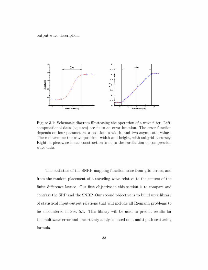
3.1 Schematic diagram illustrating the operation of a wave filter. Left:
computational data (squares) are fit to an error function. The er-
ror function depends on four parameters, a position, a width, and
two asymptotic values. These determine the wave position, width
and height, with subgrid accuracy. Right: a piecewise linear con-
struction is fit to the rarefaction or compression wave data. . . 33
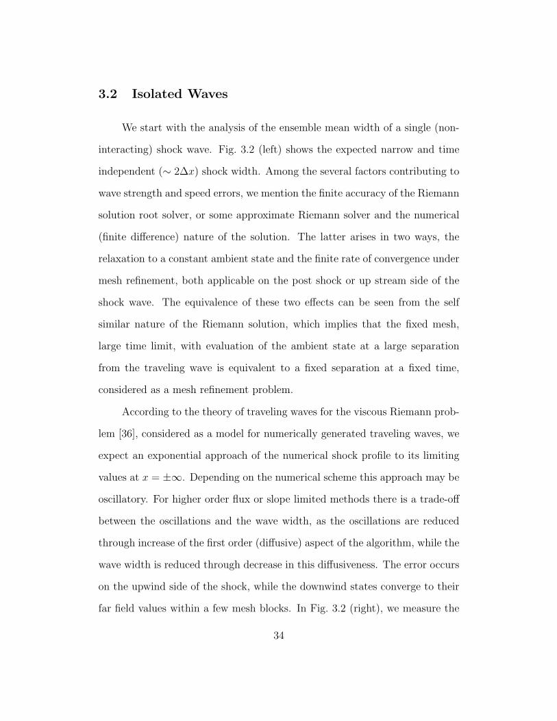
3.2 Ensemble mean shock width (the green dots on the right) and the
standard deviation (the red dots on the left) of the shock width
(left frame). The mean width, equal to about 2∆x, is much larger
than the standard deviation, indicating that the mean width is
essentially a deterministic feature of the solution. Convergence
properties of the traveling wave to the steady state values on
each side of the wave (right frame). The straight line in the right
frame is the asymptote to the exponential convergence rate, with
slope 0.01 in units of ∆x. . . . . . . . . . . . . . . . . . . . . . 35
3.3 Ensemble mean contact width for isolated noninteracting waves.
Because the width is entirely grid related, we record width in units
of ∆x and time in units of the number of time steps. The standard
deviations are also plotted as the red points to the extreme left in
each frame. Left (step down): we observe an increase from 2 cells
to 30 over 104 steps and an asymptotic growth rate cct1/3, where
cc ∼ 1 depends on the flow Mach number. The straight line in
the left frame is the asymptote to the contact width, with slope
3. Right (step up): We observe a bound on the contact width. 37
x

3.4 Ensemble mean shock and contact position errors as a function
of time, expressed in grid units. Step up case. In the label, B.S.:
Backward Shock, C: Contact, F.S.: Forward Shock. . . . . . . . 42
3.5 Ensemble mean shock and contact position errors as a function of
time, expressed in grid units. To emphasize the transient errors,
a smaller number of time steps are shown. Left: shock crossing
shock case. Right: shock crossing contact (step down) case. . . 43
3.6 Problem 3: Contact-shock (step down). . . . . . . . . . . . . . . 45
4.1 Left. Space time density contour plot for the multiple wave in-
teraction problem studied in this section, in spherical geometry.
Right. Type and location of waves determined by the wave filter
analysis. For both plots, R indicates the radius distance from the
origin. And B.S.: Backward Shock, C: Contact, and F.S.:Forward
Shock in the label. . . . . . . . . . . . . . . . . . . . . . . . . . 48
4.2 Left. Mach number vs radius for a single inward propagating
shock. Right. The same data plotted on log-log scale. . . . . . . 50
4.3 Left. Mach number vs radius for a single outgoing propagating
shock. Right. The same data plotted on log-log scale. . . . . . . 51
4.4 Ensemble mean contact width for single propagating contact. We
record width in units of ∆x. The standard deviations are also
plotted. and are the points to the extreme left in the frame. . . 52
xi

4.5 Left: ensemble mean inward/outward moving shock and contact
widths after a shock contact interaction. Right: ensemble mean
shock and contact position errors as a function of time, expressed
in grid units. The associated standard deviations are extremely
small, not shown in the plots. In the legend, C. denotes the
contact while I.S. and O.S. are the inward and outward moving
shocks. . . . . . . . . . . . . . . . . . . . . . . . . . . . . . . . . 55
5.1 The solution and its errors at the point (x, t) can be obtained
by “adding up” the solution and errors for the waves within the
domain of dependence . . . . . . . . . . . . . . . . . . . . . . . 64
5.2 Schematic graphs illustrating all contributions to the errors or
uncertainty in the output from a single Riemann solution, namely
the reshock interaction (case 3) of the reflected shock from the
wall as it crosses the contact. The numbers labeling the black
circles refer to the Riemann interactions contributing to the error.
The letter I in the first two diagrams indicates input uncertainty. 66
5.3 Schematic graphs, showing all six wave diagram contributions to
the errors or uncertainty in the output from a single Riemann
solution, namely the reshock interaction (numbered 3 in the right
frame of Fig. 4.1) of the reflected shock from the origin as it
crosses the contact. . . . . . . . . . . . . . . . . . . . . . . . . . 76
5.4 Pie charts showing the contribution of each wave interaction dia-
gram to the error variance of the wave strength at the output of
interaction 3, for a solution using 500 mesh units. . . . . . . . . 80
xii
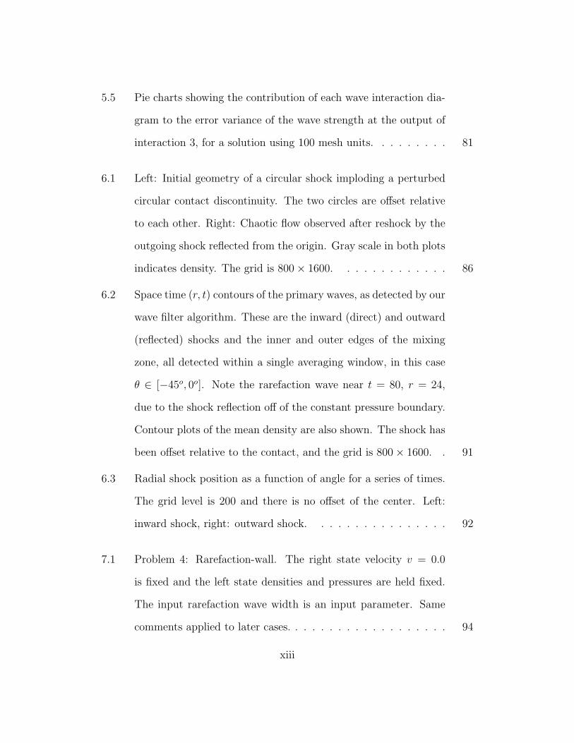
5.5 Pie charts showing the contribution of each wave interaction dia-
gram to the error variance of the wave strength at the output of
interaction 3, for a solution using 100 mesh units. . . . . . . . . 81
6.1 Left: Initial geometry of a circular shock imploding a perturbed
circular contact discontinuity. The two circles are offset relative
to each other. Right: Chaotic flow observed after reshock by the
outgoing shock reflected from the origin. Gray scale in both plots
indicates density. The grid is 800 × 1600. . . . . . . . . . . . . 86
6.2 Space time (r, t) contours of the primary waves, as detected by our
wave filter algorithm. These are the inward (direct) and outward
(reflected) shocks and the inner and outer edges of the mixing
zone, all detected within a single averaging window, in this case
θ ∈ [−45o, 0o]. Note the rarefaction wave near t = 80, r = 24,
due to the shock reflection off of the constant pressure boundary.
Contour plots of the mean density are also shown. The shock has
been offset relative to the contact, and the grid is 800 × 1600. . 91
6.3 Radial shock position as a function of angle for a series of times.
The grid level is 200 and there is no offset of the center. Left:
inward shock, right: outward shock. . . . . . . . . . . . . . . . 92
7.1 Problem 4: Rarefaction-wall. The right state velocity v = 0.0
is fixed and the left state densities and pressures are held fixed.
The input rarefaction wave width is an input parameter. Same
comments applied to later cases. . . . . . . . . . . . . . . . . . . 94
xiii

7.2 Problem 5: Contact-rarefaction. The right state velocity v = 0.0
is fixed and the left state densities and pressures are held fixed. 95
7.3 Problem 6: Shock-shock overtake (two waves of the same family).
The left state is held fixed and the two wave strengths are varied. 97
7.4 Because the width is entirely grid related, we record width in
units of ∆x and time in units of the number of time steps. . . . 98
7.5 Problem 7: Compression-wall. The right state is held fixed. . . . 99
7.6 Problem 8: Contact-compression. The right state velocity v = 0.0
is fixed and the left state densities and pressures are held fixed. 101
7.7 Problem 9: Rarefaction-wall. The right state velocity v = 0.0 is
fixed and the left state densities and pressures are held fixed. . . 101
7.8 Problem 10: Contact-rarefaction. The right state velocity v = 0.0
is fixed and the left state densities and pressures are held fixed. 103
xiv
List of Tables
2.1 The shock-contact (step up) interaction. Expansion coefficients
for output wave strengths for input variation ±10%. Compari-
son of linear, bilinear, and full quadratic models for the output
variables wok. . . . . . . . . . . . . . . . . . . . . . . . . . . . . . 22
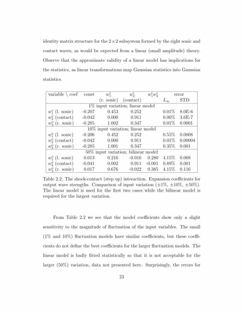
2.2 The shock-contact (step up) interaction. Expansion coefficients
for output wave strengths. Comparison of input variation (±1%,
±10%, ±50%). The linear model is used for the first two cases
while the bilinear model is required for the largest variation. . . 23
2.3 The shock crossing equal shock (wall reflection) interaction. Ex-
pansion coefficients for output wave strengths (linear model) for
input variation ±10%. . . . . . . . . . . . . . . . . . . . . . . . 24
3.1 The SNRP shock contact (step up) interaction. Expansion coeffi-
cients for output wave strengths (linear model) for input variation
±10%. Here the base case input contact wave width is zero. . . 40
3.2 The SNRP defined by the crossing of two shocks. Expansion
coefficients for output wave strengths, widths and position errors
(linear model) for input variation ±10%. . . . . . . . . . . . . . 44
xv

3.3 The SNRP shock contact (step down) interaction. Expansion
coefficients for output wave strengths, widths and position errors
(linear model) for input variation ±10%. . . . . . . . . . . . . . 46
4.1 Comparison of the exponents from the approximate and the exact
similarity solutions. . . . . . . . . . . . . . . . . . . . . . . . . . 49
4.2 The SNRP shock contact interaction. Expansion coefficients for
output wave strengths, wave strength errors, wave width errors
and wave position errors (linear model) for the initial shock con-
tact interaction. Here the base case input contact wave width
is zero. The final columns refer to difference between the linear
model (2.1) and the exact quantity. The errors in rows 4-12 refer
to the difference between the numerical solution on 100 cells and
the exact solution using 2000 cells. . . . . . . . . . . . . . . . . 58
4.3 The SNRP defined by the shock reflection at the origin. Expan-
sion coefficients for output wave strengths, wave strength errors,
wave width errors and wave position errors (linear model) for in-
put variation ±10%. . . . . . . . . . . . . . . . . . . . . . . . . 59
4.4 The SNRP contact reshock interaction. Expansion coefficients for
output wave strengths, wave strength errors, wave width errors
and wave position errors (linear model). . . . . . . . . . . . . . 60
5.1 Predicted and simulated errors for output wave strengths, wave
widths and wave positions, Case 1. . . . . . . . . . . . . . . . . 70
xvi

5.2 Predicted and simulated errors for output wave strengths, wave
widths and wave positions, Case 2. . . . . . . . . . . . . . . . . 71
5.3 Predicted and simulated errors for output wave strengths, wave
widths and wave positions, Case 3. . . . . . . . . . . . . . . . . 72
5.4 Case 1. The contact-shock interaction (step up). Errors for out-
put wave strengths, wave widths and wave position. Comparison
of under resolved simulation and prediction. . . . . . . . . . . . 73
5.5 Case 2. The shock crossing equal shock (wave reflection) inter-
action. Errors for output wave strengths, wave width and wave
position. Comparison of under resolved simulation and prediction. 74
5.6 Case 3. The contact-shock interaction (step down). Errors for
output wave strengths, wave width and wave position. Compari-
son of under resolved simulation and prediction. . . . . . . . . . 75
5.7 Predicted and simulated errors for output wave strengths, wave
widths and wave positions, output to interaction 3. The inward
rarefaction and contact strengths are expressed dimensionlessly as
Atwood numbers. The outward shock strengths are in the units of
Mach number. The width and position errors are in mesh units.
The wave strength errors are expressed as mean ± 2σ where σ is
the ensemble STD of the error/uncertainty. . . . . . . . . . . . 78
xvii

5.8 The contribution of each interaction to the mean value of the total
error in each of three output waves at the output to interaction 3,
for 100 and 500 mesh units. Units are dimensionless and represent
the error expressed as a fraction of the total wave strength. The
last two rows compare the total of the mean error as given by the
model to the directly observed mean error. The columns I.R., C.,
and O. S. are labeled as in Fig. 4.1, Right frame. . . . . . . . . . 79
7.1 Case 4. The SNRP defined by the crossing of two rarefactions.
Expansion coefficients for output wave strengths (linear model)
for input variation ±10%. . . . . . . . . . . . . . . . . . . . . . 95
7.2 Case 5. The SNRP defined by the contact rarefaction interaction.
Expansion coefficients for output wave strengths (linear model)
for input variation ±10%. . . . . . . . . . . . . . . . . . . . . . 96
7.3 Case 6. The SNRP defined by the shock shock overtake (two
waves of the same family). Expansion coefficients for output wave
strengths (linear model) for input variation ±10%. . . . . . . . . 99
7.4 Case 7. The SNRP defined by the crossing of two compressions.
Expansion coefficients for output wave strengths (linear model)
for input variation ±10%. . . . . . . . . . . . . . . . . . . . . . 100
7.5 Case 8. The SNRP defined by the contact compression inter-
action. Expansion coefficients for output wave strengths (linear
model) for input varation ±10%. . . . . . . . . . . . . . . . . . 102
xviii
7.6 Case 9. The SNRP defined by the crossing of two rarefactions.
Expansion coefficients for output wave strengths (linear model)
for input variation ±10%. . . . . . . . . . . . . . . . . . . . . . 102
7.7 Case 4. The crossing of two rarefactions. Predicted and simulated
errors for output wave strengths, wave widths and wave positions. 104
7.8 Case 5. The contact rarefaction interaction. Predicted and sim-
ulated errors for output wave strengths, wave widths and wave
positions. . . . . . . . . . . . . . . . . . . . . . . . . . . . . . . 105
7.9 Case 6. The shock shock overtake. Predicted and simulated errors
for output wave strengths, wave widths and wave positions. . . . 106
7.10 Case 7. The crossing of two compressions. Predicted and sim-
ulated errors for output wave strengths, wave widths and wave
positions. . . . . . . . . . . . . . . . . . . . . . . . . . . . . . . 106
7.11 Case 8. The contact compression interaction. Predicted and sim-
ulated errors for output wave strengths, wave widths and wave
positions. . . . . . . . . . . . . . . . . . . . . . . . . . . . . . . 107
7.12 Case 9. The crossing of two rarefactions. Predicted and simulated
errors for output wave strengths, wave widths and wave positions. 107
7.13 Case 4. The crossing of two rarefactions. Predicted and simulated
errors for output wave strengths, wave widths and wave positions.
Comparison of under resolved simulation and prediction. . . . . 108
7.14 Case 5. The contact rarefaction interaction. Predicted and sim-
ulated errors for output wave strengths, wave widths and wave
positions. Comparison of under resolved simulation and prediction.108
xix
7.15 Case 6. The shock shock overtake. Predicted and simulated er-
rors for output wave strengths, wave widths and wave positions.
Comparison of under resolved simulation and prediction. . . . . 109
7.16 Case 7. The crossing of two compressions. Predicted and sim-
ulated errors for output wave strengths, wave widths and wave
positions. Comparison of under resolved simulation and prediction.109
7.17 Case 8. The contact compression interaction. Predicted and sim-
ulated errors for output wave strengths, wave widths and wave
positions. Comparison of under resolved simulation and prediction.110
7.18 Case 9. The crossing of two rarefactions. Predicted and simulated
errors for output wave strengths, wave widths and wave positions.
Comparison of under resolved simulation and prediction. . . . . 110
xx

Acknowledgements
My thanks go to everyone who has been involved in making me into this
picture.
I would like to extend my deepest gratitude and thanks to James Glimm,
my adviser, for his insightful suggestions and constant support throughout my
research. I often felt fortunate to be under his advisement, as a great math-
ematician and brilliant physicist, he not only gave guidance on my scientific
research, but also set up a lifetime role model to follow. I am also thankful to
Xiaolin Li for his authentic encouragement, which led me through the early
years of chaos and confusion.
Professor Kenny Ye has been deeply involved in the early stage of this
project, he has led me through the door of the practical statistical data analy-
sis. Professor Wei Zhu expressed her interest in my work and shared with me
her knowledge of statistics and provided many useful references and friendly
encouragement. Professor Stephen Finch and David G. Ebin, thank you for
your valuable suggestion and sincere comments for the completion of this dis-
sertation.
I should also mention that my graduate studies in Stony Brook were
supported by NSF and the U. S. Department of Energy. Their support makes

research like this possible.
Of course, I am most grateful to my parents, who have been always
supportive to whatever decisions that came to me, and their unconditional
love. Without them this work would never have come into existence (literally).
Finally, I wish to thank the following the most: Yan Yu, Taewon Lee(for
our four years’ friendship and collaboration on this project to make this thesis
complete); Jean Nick Pestieau and Wurigen Bo (for their later contributions
into this project); my most special friend Fay Y. Zhao (for all your support and
care); Xiaofei Fan, Masha Prodanovic, Dasha Eremina, Hyunsun Lee, So-Youn
Shin, Xiangfeng Wu ... (for all the good and bad times we had together).
xxii
Chapter 1
Introduction and Background
1.1 Uncertainty Quantification
Uncertainty quantification is at its essence a study of errors, both their
description and their consequences. Addressed here are the errors arising from
the finite resolution numerical discretization used to obtain solutions. In this
sense, the problem, a bit simplistically, can be viewed as the determination of
error bars to be assigned to the numerical solution algorithms. For a Bayesian
decision framework which leads to this point of view see [19–21]. Unlike other
authors [3, 5, 8, 24, 26] who usually use observational errors or expert opinions
[8] to form the probability model for the likelihood, our approach is to use
solution error models for the likelihood. We provide a scientific basis for the
probabilities associated with numerical solution errors. The authors are not
aware of comparable error analysis studies, but of course numerical simulation
errors have been long studied from different points of view.
An early focus of numerical error modeling was round off errors. For the
hyperbolic systems we study, modern 64-bit processors with double precision
1

arithmetic appear, as a practical matter, not to be sensitive to this class of
errors, while they are difficult to analyze theoretically. A common approach to
error analysis in numerical analysis is the study of the asymptotic behavior of
errors under mesh refinement. The method of asymptotic analysis of numerical
solution errors is so old and well established that it is difficult to cite its origins
[32]. This is a useful approach, and one we refer to in the case of well resolved
simulations. However, since many simulations are under resolved, as used in
practice, asymptotic analysis of convergence does not address the issue of error
bars and uncertainty quantification. Moreover, the coefficients which multiply
powers of ∆x in the asymptotic expressions cannot be determined theoreti-
cally. A third main theme in the analysis of errors is the use of a posteriori
error estimators. The method of a a posteriori analysis aims to construct an
upper bound on the solution error, either theoretically validated or based on
numerical experiments [2, 7, 28, 31]. But for hyperbolically dominated flows,
with poor theoretical foundations, a posteriori methods are generally inap-
plicable. We seek to characterize the error, not just to bound it. Moreover,
a posteriori methods are most fully developed and justified theoretically for
elliptic problems, and have only a partial or preliminary development for the
shock interaction problems we consider here. For this reason, we consider er-
rors from a statistical point of view, and examine an ensemble of coarse and
fine grid pairs, and their differences, which are assumed to represent the coarse
grid solution error.
We have developed an approach to uncertainty quantification for numer-
ical simulations that is based on three ideas:
2

1. A combined approach for forward as well as inverse propagation of un-
certainty [19, 20]. This combined approach is important when the use of
disparate sources of data, including data pertaining to observations of
full system performance, is important.
2. Models for numerical solution errors [9, 16–18]. For multi-scale problems
and complex multi-physics problems, under-resolved simulations and ac-
companying simulation error are frequently unavoidable in practice.
3. Parametrization, comprehensibility, and validation of simulation error
models [15]. This step allows testing and validation to occur in somewhat
idealized situations, less complex than the full system simulations, but
still applicable to them.
Our principal concern is to develop a method for determining solution
errors in shock wave interaction problems having a significant degree of com-
plexity. Our strategy takes advantage of the fact that shock problems typically
consist of smooth regions separated by discontinuities (actually narrow regions
with strong solution gradients), and consists of three main steps.
Step 1: Determine solution errors for a comprehensive set of elementary wave
interactions. These are summarized as a set of input/output relations
for the errors in such interactions;
Step 2: Construct wave filters that decompose a complex flow into approximately
independent components consisting of elementary waves;
3
Step 3: Formulate a composition law that constructs the total solution error at
any space-time point in terms of errors from repeated elementary inter-
actions.
Step 1 is carried out in Chap. 2, 3 and 4. Step 2 is discussed in [25]. The
main idea is summarized and extended in Chap. 3 and 4. The composition
law is presented in Chap. 5.
We validate this method by predicting the errors in the composite (com-
plex) simulation with the errors calculated using the composition law [10]. The
results are derived by a study of errors in the solution of Riemann problems,
for details see Sec. 1.2.1.
The uncertainty of a numerical simulation comes from three different
sources, the errors in the physical model, the errors in the numerical model
(ı.e. simulation errors), and the uncertainty on the input parameters of the
model(ı.e. initial uncertainty). In our study, we mainly focused on the latter
two categories of errors. Simulation errors typically consist of:
• position errors in the location of the traveling wave discontinuities or
sharp solution gradients;
• wave width errors arising from the numerical vs. the physical width of
the traveling waves;
• solution state errors in the smooth regions bordering the regions with
discontinuities or sharp solution gradients.
Any or all or these errors may arise in the input data to the Riemann
problem. Output errors, however, have two sources. Those arising from inac-
4
curacies in the solution algorithm are called created errors, while those that
can be ascribed directly to input error or uncertainty are called transmitted
errors or transmitted uncertainty.
In contrast to the case of planar waves, the complications that addition-
ally result from spherical geometry are the following:
1. The solution waves are not of constant strength between wave interac-
tions, but evolve approximately according to a power law as a function
of the radius.
2. The solution is not spatially constant between waves.
The radially dependent strength of spherical waves is discussed in [36]. The
spatial variation of spherical waves is contained in the Guderley solution [22],
which gives simple power laws that predict this dependence of the solution on
the radius. We find that these power laws also predict the evolution of the
error, which, once formed, propagates according to the same laws as govern
the solution the waves themselves.
In summarizing and extending the results of [25], we also introduced
diagnostic windows, which measure the solution state in the constant regions
between the waves, as well as window filters, which identify individual wave
types (The filters look for regions containing one single wave passing through
the filter).
5
1.2 Background
1.2.1 1D Simulation Formulation
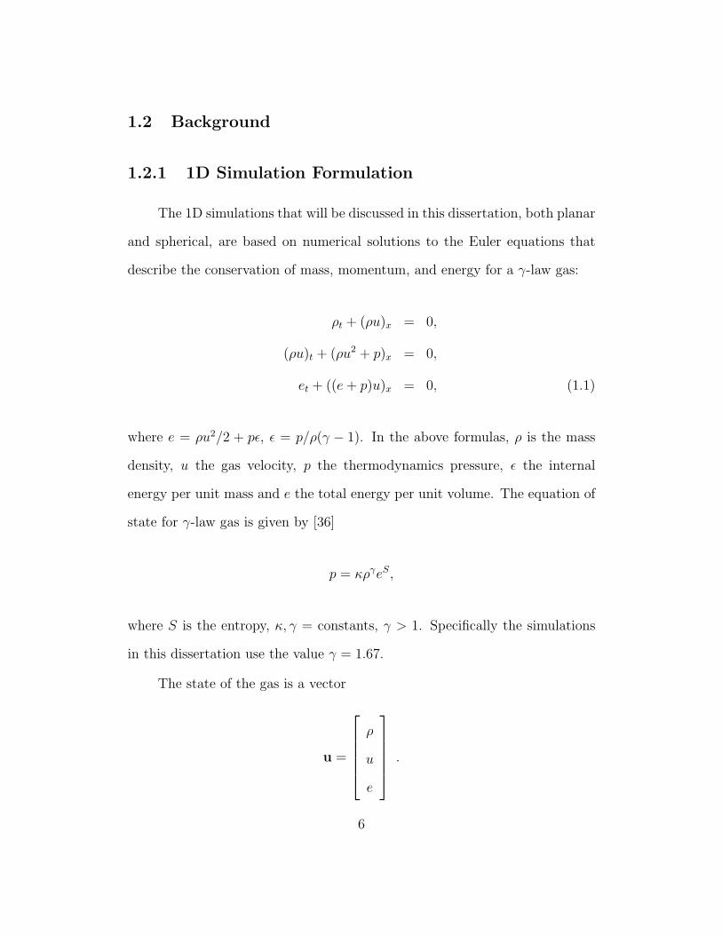
The 1D simulations that will be discussed in this dissertation, both planar
and spherical, are based on numerical solutions to the Euler equations that
describe the conservation of mass, momentum, and energy for a γ-law gas:
ρt + (ρu)x = 0,
(ρu)t + (ρu2 + p)x = 0,
et + ((e + p)u)x = 0, (1.1)
where e = ρu2/2 + pε, ε = p/ρ(γ − 1). In the above formulas, ρ is the mass
density, u the gas velocity, p the thermodynamics pressure, ε the internal
energy per unit mass and e the total energy per unit volume. The equation of
state for γ-law gas is given by [36]
p = κργeS,
where S is the entropy, κ, γ = constants, γ > 1. Specifically the simulations
in this dissertation use the value γ = 1.67.
The state of the gas is a vector
u =
⎡⎢⎢⎢⎢⎣
ρ
u
e
⎤⎥⎥⎥⎥⎦ .
6
The Riemann problem [6] is the initial value problem for equation 1.1 with
special initial data of the form
u(x, 0) =
⎧⎪⎨⎪⎩
ur, x ≥ 0,
ul, x ≤ 0,
where
ur =
⎡⎢⎢⎢⎢⎣
ρr
ur
er
⎤⎥⎥⎥⎥⎦ and ul =
⎡⎢⎢⎢⎢⎣
ρl
ul
el
⎤⎥⎥⎥⎥⎦
are two constant states of the gas. The solutions of Riemann problem will be
made up of three types of elementary waves (solutions) in the region t > 0.
We define c as speed with c2 = γp/ρ. Characteristics for a simple wave
are
C+ :dx
dt= u + c and C− :
dx
dt= u − c .
Riemann invariants are found to be
Γ± = u ±∫
c(ρ)
ρdρ.
Γ± are constant along the characteristics C±, respectively.
At a point where the solution has a jump discontinuity propagating with
7

the speed s = dx/dt, the Rankine-Hugoniot jump conditions
s[ρ] = [ρu],
s[ρu] = [ρu2 + p],
s[e] = [(e + p)u],
corresponding to Eq. 1.1 must hold; these jump conditions reflect conservation
of mass, momentum, and energy through the discontinuity. Here the jump [A]
in a quantity A is defined by [A] = A+ − A−, where A± is the limiting value
of A on the right(left) of the discontinuity.
Pick a coordinate system in which the discontinuity stays stationary. In
this coordination system, the Rankine-Hugoniot relations at the origin become
ρ1u1 = ρ0u0,
ρ1u21 + p1 = ρ0u
20 + p0,
(e1 + p1)u1 = (e0 + p0)u0. (1.2)
Let mass flux M = ρ1u1 = ρ0u0. If M = 0 we call the discontinuity a
contact-discontinuity. u1 = u0 = 0, which indicates the discontinuity moves
with the flow, p1 = p0, ρ1 �= ρ0.
If M �= 0, this discontinuity is called a shock. With subscript 0/1 indicate
the states in the front/back of shock, respectively. We can derive some simple
8
identities from Eqs. 1.1 and 1.2:
M2 = −p0 − p1
ν0 − ν1
,
u0u1 =p0 − p1
ρ0 − ρ1
,
ε1 − ε0 +p0 + p1
2(ν1 − ν0) = 0,
where ν = 1/ρ, and the third equation is called Hugoniot equation for the
shock.
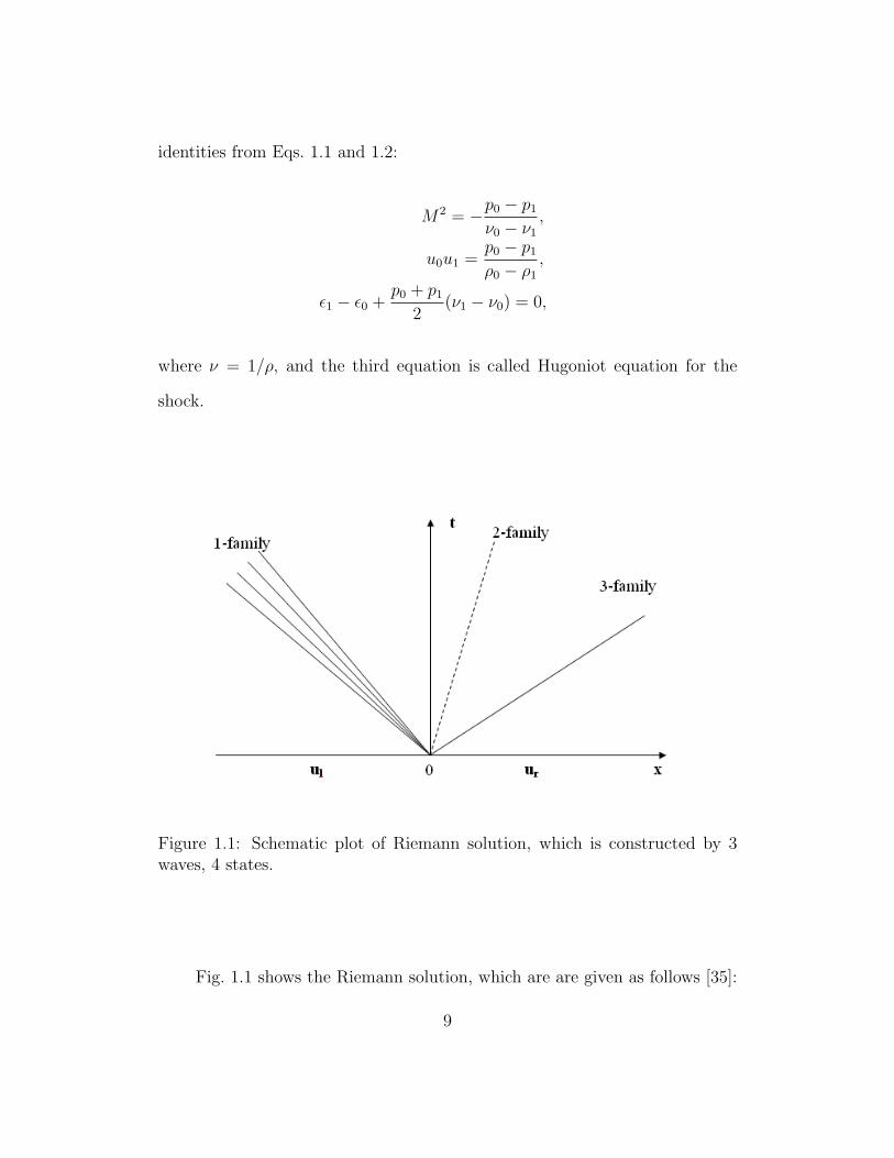
Figure 1.1: Schematic plot of Riemann solution, which is constructed by 3waves, 4 states.
Fig. 1.1 shows the Riemann solution, which are are given as follows [35]:
9
1-family
pr/pl = e−x ,
ρr/ρl = f1(x) ≡
⎧⎪⎨⎪⎩
e−x/y, x ≥ 0,
β+ex
1+βex , x ≤ 0,
(ur − ul)/cl = h1(x) ≡
⎧⎪⎨⎪⎩
2(1 − e−τx)/(γ − 1), x ≥ 0,
2√
τ(1−e−x)
(γ−1)(1+βe−x)1/2 , x ≤ 0,
2-family
pr/pl = 1, ρr/ρl = ex, ur − ul = 0;
3-family
pr/pl = ex ,
ρr/ρl = f3(x) ≡ 1/f1(x),
(ur − ul)/cl = h3(x) ≡
⎧⎪⎨⎪⎩
2(eτx − 1)/(γ − 1), x ≥ 0,
2√
τ(ex−1)
(γ−1)(1+βex)1/2 , x ≤ 0,
where constants β = (γ + 1)/(γ − 1), τ = (γ − 1)/2γ.
For equations of state 1.1, there is a unique solution (in the class of shocks,
centered simple waves, and contact discontinuities separating constant states)
to the Riemann problem with these initial states, if and only if
ur − ul <2
γ − 1(cl + cr). (1.3)
If 1.3 is violated, then a vacuum is present in the solution [35]. We define
10
A = ρr/ρl, B = pr/pl, and C = (ur − ul)/cl, then the following hold given the
condition 1.3:
1. The 1-family of the solution is a simple wave if and only if
√2
γ − 1h1logB < C <
2
γ − 1
[1 +
√B
A
],
and is a shock otherwise
2. The 3-family of the solution is a simple wave if and only if
h1(−logB) < C <2
γ − 1
[1 +
√B
A
],
and is a shock otherwise.
Illustrations of the setup specifications for the base case of one dimen-
sional planar geometry simulation are given in Fig. 2.1 of Chap. 2. Reflecting
boundary conditions are applied at both x = 0 and x = xmax (r = 0 and
r = rmax in spherical geometry).
1.2.2 Introduction to FronTier
Since our work is based on numerical simulations using the FronT ier
code, we also present a brief introduction to this code.
The FronT ier code is based on front tracking, a numerical method which
regards the fluid interface as an evolving, lower dimensional mesh. The Front
Tracking method, initiated by Richtmyer and Morton [33], is designed to pro-
vide piecewise smooth solutions as well as distinguished discontinuities which
11

separate the smooth solutions in solving systems of hyperbolic partial differ-
ential equations. Fig. 1.2 is a flow chart taken from [13] describing the front
tracking computation in FronT ier. For more details, see [12–14].
1.3 Organization of This Dissertation
In the Chap. 1, the concept of uncertainty quantification was introduced.
We then discussed our general steps to address uncertainty quantification prob-
lems in numerical solutions, which, to be specific, are error analysis. A back-
ground review of FronT ier code and Front Tracking algorithm used for our
numerical simulations was also given.
In Chap. 2 we studied the statistical Riemann problem (SRP), which is
to describe the non-linear problem of the interaction of strong hydrodynamic
waves by our simple linear input-output models. Statistical Riemann problems
are illustrated to show how to map the distributions of errors from input to
output.
In Chap. 3 we study the statistical numerical Riemann problem (SNRP).
This differs from the statistical Riemann problem in that incoming shock
waves, specified numerically, have finite width determined from numerical as
well as physical considerations. We note that incoming rarefaction and com-
pression waves have physical time dependent widths. The SNRP also differs
in that the numerical algorithm that solves the Riemann problem creates (as
well as propagates) errors. We will show that, to fairly good accuracy, one
can model the errors in the outgoing waves as affine linear, i.e., constant plus
linear, (or perhaps bilinear) statistical expressions in the strength of the incom-
12
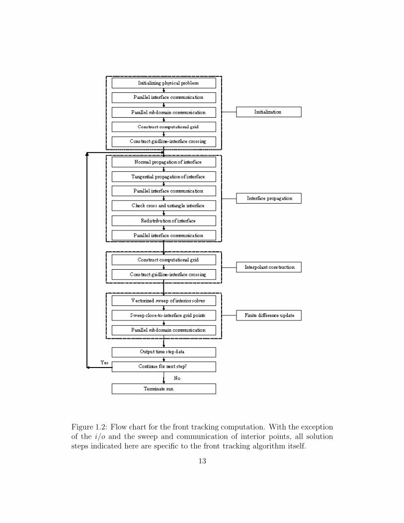
Figure 1.2: Flow chart for the front tracking computation. With the exceptionof the i/o and the sweep and communication of interior points, all solutionsteps indicated here are specific to the front tracking algorithm itself.
13
ing waves. The coefficients in these linear expressions depend parametrically
on the incoming waves, and here they are taken as defined by a character-
istic of base case. Diagnostic window and wave filters were introduced. A
wave filter is an automated pattern recognition algorithm which locates shock
wave, rarefaction wave and contact discontinuities in numerical solutions of the
Euler equations for compressible fluids. These filters locate the shock waves
and identify wave widths. Based on these wave filters, we can also study the
behavior of isolated waves.
Chap. 4 led our discussion of SNRP into 1D spherical flows. The spherical
geometry complicated our previous models by a nonconstant power law growth
or decay of error between interactions.
A composition law for complex 1D shock wave interaction problems was
elaborated in Chap. 5 in both planar and spherical geometry, based on our
detail studies of SNRP in Chap. 3 and Chap. 4.
Several conclusions for uncertainty quantification studies in 1D flows were
presented in Chap. 6. Also in this chapter, some open problems in 2D chaotic
flows were discussed, which are our future work.
The rest 7 (besides the 3 modeled in Chap. 3) of the 10 Riemann Problems
showed in Fig. 2.4 are modeled as SNRP and presented in the Appendix 7.1.
The continued error study of later interactions for both resolved and under
resolved calculation can also be found in the Appendix 7.2.
14
Chapter 2
Statistical Riemann Problems
The main result of this chapter is that a linear input-output model will
serve to describe the manifestly nonlinear problem of the interaction of strong
hydrodynamic waves.
In this chapter, the solution operator is considered to be exact, and acts
to propagate the input error (or uncertainty) to the output error. The out-
put errors can be represented conceptually as a multinomial in powers of the
strengths of the waves that are interacting. We characterize the statistics of
the errors as Gaussian, and thus the error distribution is determined by its
mean and covariance. For weak waves these quantities (mean and covariance)
as a description of the input, are transformed via the solution operator Ja-
cobean to the mean and covariance of the output. We are more interested in
strong waves, but find a description of the solution operator as linear pertur-
bation about base case still provides a useful description of the input to output
transformed error statistics.
We consider, in one spatial dimension, the interaction of a shock wave
15
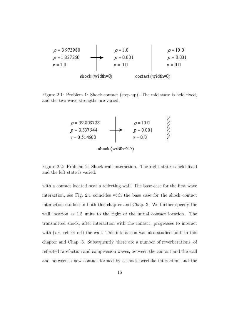
Figure 2.1: Problem 1: Shock-contact (step up). The mid state is held fixed,and the two wave strengths are varied.
Figure 2.2: Problem 2: Shock-wall interaction. The right state is held fixedand the left state is varied.
with a contact located near a reflecting wall. The base case for the first wave
interaction, see Fig. 2.1 coincides with the base case for the shock contact
interaction studied in both this chapter and Chap. 3. We further specify the
wall location as 1.5 units to the right of the initial contact location. The
transmitted shock, after interaction with the contact, progresses to interact
with (i.e. reflect off) the wall. This interaction was also studied both in this
chapter and Chap. 3. Subsequently, there are a number of reverberations, of
reflected rarefaction and compression waves, between the contact and the wall
and between a new contact formed by a shock overtake interaction and the
16
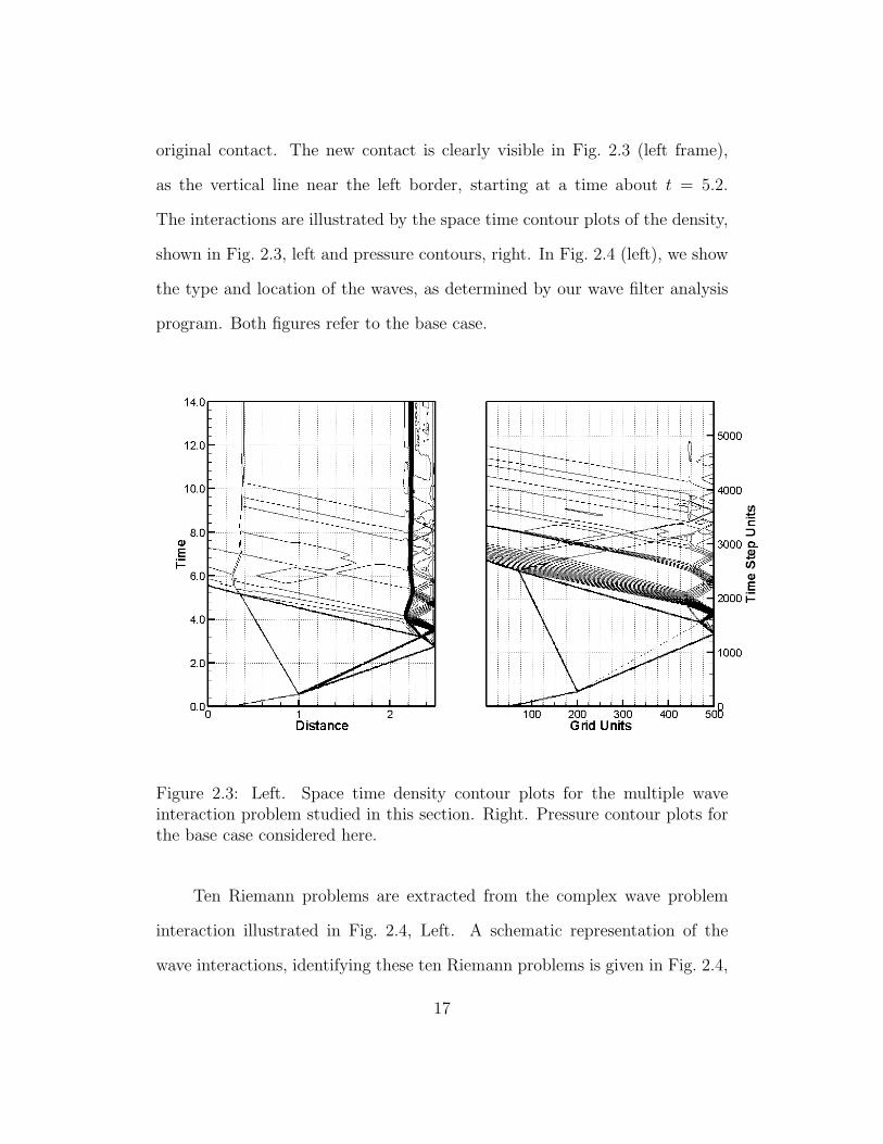
original contact. The new contact is clearly visible in Fig. 2.3 (left frame),
as the vertical line near the left border, starting at a time about t = 5.2.
The interactions are illustrated by the space time contour plots of the density,
shown in Fig. 2.3, left and pressure contours, right. In Fig. 2.4 (left), we show
the type and location of the waves, as determined by our wave filter analysis
program. Both figures refer to the base case.
Figure 2.3: Left. Space time density contour plots for the multiple waveinteraction problem studied in this section. Right. Pressure contour plots forthe base case considered here.
Ten Riemann problems are extracted from the complex wave problem
interaction illustrated in Fig. 2.4, Left. A schematic representation of the
wave interactions, identifying these ten Riemann problems is given in Fig. 2.4,
17

Figure 2.4: Left: Type and location of waves as determined by our wave filteranalysis for the base case considered here. Right: Schematic representationof the waves and the interactions, with labels for the interactions, taken fromthe left frame.
Right.
2.1 A Multinomial Expansion for the SRP Output
The SRP considered here has two incoming waves, each of which may be
one of the followings: contact, shock, rarefaction, or compression. Rarefaction
and compression waves only interact when they belong to opposite families,
while two contacts never interact. For pairwise interactions (shock interactions
with other shocks, with rarefaction or with compression waves), we distinguish
18

whether the two interacting waves are of the same (left moving vs. right
moving) family or opposite families. For contact waves, we specify the direction
of the density change (step up or down) as seen from the side of the wave
approaching the contact. Thus there are a total of 14 elementary cases for the
incoming waves. Each case is associated with a wave amplitude of a specific
sign, so that there is no loss of generality in assuming that the signs are chosen
so that the amplitudes are non-negative. Fixing one case, we specify a starting
state for the incoming waves, and a base case for the (strong) wave strengths.
Then we consider variation about this base case by ±1%, ±10% and ±50% in
the density ratio (for contacts) or pressure (for all other waves). Within this
formulation, we can describe the output wave strengths by an expression linear
in the two input wave strengths, with a possible additional bilinear term, i.e.
linear in the the product of the input wave strengths.
The range of validity of such a bilinearization will depend on the details
of how the problem is formulated; perhaps the most important factor is the
choice of variables to describe wave strengths. We choose two dimensionless
variables to measure these wave strengths; a modified Atwood number A =
(ρ2−ρ1)/(ρ02 +ρ0
1) to measure contact strengths, and a similar expression built
out of the pressures, P = (P2 −P1)/(P02 +P 0
1 ), for the other wave types. Here
the quantities ρ0i and P 0
i denote densities and pressures from the base case
associated with the ensemble. Of course the solution of a Riemann problem,
being fully nonlinear, will require an infinite Taylor’s series for its complete
description. Terms in the series expansion can be determined by statistical
study, which is fit to linear/bilinear regression models for a given finite sample
19

size.
However, this statistical test misses the point and the value of a simple
model. We want to capture the main effects, and regard the remainder not
as a statistical sampling error but as a modeling error. Thus we consider an
expansion with more terms than we ultimately want, and discard terms with
small coefficients even if the associated p-value is not near 1. For input wave
strengths wi1, wi
2 (i ≡ in) and output wave strengths wo1, wo
2 and wo3 (o ≡ out)
(ordered from left to right in real 1D space), the expansion is defined by its
coefficients αk,J , for J a multi index, J = (j1, j2). The expansion has the form
wok =
∑J
αk,Jwi,J , (2.1)
where wi,J = (wi1)
j1(wi2)
j2 . The coefficients αk,J depend parametrically on the
base case Riemann problem. Given a statistical ensemble of input and output
values wi and wo, we use a least squares algorithm to determine the best
fitting model parameters αk,J , for any given polynomial order of model. We
use (2.1) variationally, that is to map input variation (about the base case for
the ensemble) to output variability. In other words, (2.1), which is a formula
for wave strengths, implies a similar formula with different but computable
coefficients αk,J , in which all ω’s are defined as variations from the base case,
so that they represent uncertainty or error. For simplicity we consider the case
of a linear input-output relation, ωok = αk,0 +
∑J αk,Jωi,J . If we denote the
base case with an overbar, i.e. ωok and ωi,J , then the fluctuation δωo
k = ωok−ωo
k
satisfies δωok =
∑J αk,Jδωi,J .
20

2.2 Evaluation of the Expansion Coefficients
The main point of this section is to determine numerical values for the
expansion coefficients of the output wave strengths of the SRP. We also find
that, for many cases, the linear model is sufficient for scientific accuracy, while
the case of large variability will likely require additional expansion terms. We
show that bilinear terms are sufficient for large variability.
We consider, as a typical Riemann problem, the wave interaction of a
shock wave moving (to the right) into a contact (density increase, or step up
case). This wave interaction initiates the complex series of interactions studied
in Sec. 5.1.
The base case shock strength is given with a pressure ratio P2/P1 = 1337
(P = 0.999), and contact density ratio ρ2/ρ1 = 10 (A = 0.82). The equation
of state satisfies a gamma law gas with γ = 1.67.
Typical results on the variation of the polynomial order of the model are
presented in Table 2.1, while results for variation of the strength of the input
waves are shown in Table 2.2. To read these tables, we note that the first
row of Table 2.1 (labeled as wo1 (l.sonic)) lists coefficients α1,J for J = (0, 0),
J = (1, 0), etc. These coefficients are determined by a least squares algorithm,
that minimizes the mean error over the ensemble predictions to the exact
solution of the Riemann problem. The last two columns describe errors in the
model (2.1). The column labeled L∞ is the maximum of the absolute value,
over the ensemble, of the relative error, and it may be sensitive to the choice
of ensemble. Note that the sample size studied here and all cases after is 200.
The relative error is defined as (predicted - exact)/exact where exact is the
21

variable \ coef const wi1 wi
2 wi1w
i2 (wi
1)2 (wi
2)2 error
(r. sonic) (contact) L∞ STDlinear response model
wo1 (l. sonic) -0.206 0.452 0.252 0.55% 0.0008
wo2 (contact) -0.042 0.000 0.911 0.01% 0.00004
wo3 (r. sonic) -0.285 1.001 0.347 0.35% 0.001
bilinear response modelwo
1 (l. sonic) 0.011 0.234 -0.015 0.267 0.16% 0.0003wo
2 (contact) -0.043 0.001 0.912 -0.001 0.01% 0.00004wo
3 (r. sonic) 0.015 0.701 -0.020 0.368 0.10% 0.01quadratic response model
wo1 (l. sonic) -0.090 0.245 0.222 0.253 0.000 -0.136 0.01% 0.00002
wo2 (contact) -0.030 0.001 0.881 0.001 0.000 0.018 0.00% 1.1E-6
wo3 (r. sonic) -0.125 0.715 0.305 0.349 0.001 -0.187 0.02% 0.00002
Table 2.1: The shock-contact (step up) interaction. Expansion coefficientsfor output wave strengths for input variation ±10%. Comparison of linear,bilinear, and full quadratic models for the output variables wo
k.
result of the (exact) Riemann solution and predicted is the value given by
the finite polynomial model. The column STD is the standard deviation of
(predicted - exact). From the small values of these errors for the linear model,
as seen in Table 2.1, we conclude that the linear model is adequate for many
purposes. The two pure quadratic columns of the quadratic model are small,
indicating that the quadratic model is basically a correction to the bilinear
model. However, the 3× 3 linear sub block of the bilinear model is not a good
approximation to the corresponding values of the linear model. Moreover, in
this case the size of the pure bilinear terms in the model is large relative to the
decrease in error achieved by use of the bilinear model relative to the linear
one. Thus we conclude that the bilinear model contains a substantial amount
of cancelation between its terms, and in general the linear model may be more
satisfactory. All three models in Table 2.1 show an approximate diagonal,
22
identity matrix structure for the 2×2 subsystem formed by the right sonic and
contact waves, as would be expected from a linear (small amplitude) theory.
Observe that the approximate validity of a linear model has implications for
the statistics, as linear transformations map Gaussian statistics into Gaussian
statistics.
variable \ coef const wi1 wi
2 wi1w
i2 error
(r. sonic) (contact) L∞ STD1% input variation; linear model
wo1 (l. sonic) -0.207 0.453 0.252 0.01% 8.0E-6
wo2 (contact) -0.042 0.000 0.911 0.00% 3.6E-7
wo3 (r. sonic) -0.285 1.002 0.347 0.01% 0.0001
10% input variation; linear modelwo
1 (l. sonic) -0.206 0.452 0.252 0.55% 0.0008wo
2 (contact) -0.042 0.000 0.911 0.01% 0.00004wo
3 (r. sonic) -0.285 1.001 0.347 0.35% 0.00150% input variation; bilinear model
wo1 (l. sonic) 0.013 0.216 -0.016 0.280 4.15% 0.008
wo2 (contact) -0.041 0.002 0.911 -0.001 0.89% 0.001
wo3 (r. sonic) 0.017 0.676 -0.022 0.385 4.15% 0.116
Table 2.2: The shock-contact (step up) interaction. Expansion coefficients foroutput wave strengths. Comparison of input variation (±1%, ±10%, ±50%).The linear model is used for the first two cases while the bilinear model isrequired for the largest variation.
From Table 2.2 we see that the model coefficients show only a slight
sensitivity to the magnitude of fluctuation of the input variables. The small
(1% and 10%) fluctuation models have similar coefficients, but these coeffi-
cients do not define the best coefficients for the larger fluctuation models. The
linear model is badly fitted statistically so that it is not acceptable for the
larger (50%) variation, data not presented here. Surprisingly, the errors for
23

the quadratic model with input 50% variation are somewhat higher than for
the bilinear. We therefore use the bilinear model for 50% variation.
variable \ coef const wi1 error
(r. sonic) L∞ STDwo
1 (l. sonic) -0.0008 0.715 0.00% 4E-8
Table 2.3: The shock crossing equal shock (wall reflection) interaction. Expan-sion coefficients for output wave strengths (linear model) for input variation±10%.
In Table 2.3 we consider the shock crossing shock case. The two waves are
of opposite families and each has Mach number 53. This case is also the second
(in time) Riemann problem to occur within the complex problem studied in
Sec. 5.1, as shock reflection from a wall.
2.3 Variance
In essence our analysis will proceed by ignoring the correlation among
output waves. Having done so, we determine the variance of the output waves
as a function of the input distributions. The formulas are first derived with
general applicability, and then specialized to our situation, including the as-
sumption of a linear input-output model.
The Riemann solution wo = W o(wi) defines a mapping from the input to
the output statistics. The approximate mapping (2.1) defines an easily com-
putable approximation to this transformation of statistics. Thus for a given
probability distribution dνi(wi) defined on the input variables, and supported
in a domain Di of input variables, the output variables lie in a domain Do,
24

and on this domain the probability measure for the output variables is
dνo(wo) =dνo(W o)
dνi(wi)dνi(ωi) . (2.2)
From the above the formula, we see an immediate problem. The three
output variables, defined as a function of the two input variables, cannot be
statistically independent. They lie in a two dimensional sub-domain, Do, of
the three dimensional space of output wave parameters. However, these waves
separate in parameter space, and to a large extent carry out separate roles in
the composite wave interaction problem studied in Sec. 5.1. Thus we want to
generate independent statistical descriptions of each of the output waves. In
practice, for all Riemann problem simulations (except those with single input
wave), we generated 2 independent input waves (using Latin Hypercube ran-
dom generating algorithm) with parameter means equal to the corresponding
base case input wave parameters. This step, of ignoring the correlations in the
statistics of the outgoing waves, assumes that the successive interactions give
rise to a de-correlation of the solution from its dependence on the earlier inter-
actions. In a strict sense this assumption is not correct, but we believe it will
give a reasonably accurate description of the final composite statistics. The
validity of this assumption will be tested in the comparison given in Sec. 5.1,
where composition of errors from interacting Riemann problems are consid-
ered. For comparison, this assumption is analogous to the introduction of the
hypothesis of molecular chaos in the derivation of the Boltzmann equation.
We next deal with the output variance in a quantitative manner under
25
the assumptions of input independence. We write the domain Do,
Do ⊆ D1o ×D2
o ×D3o , (2.3)
as a subset of its projections Dko on the three output wave strength coordi-
nate axes. A marginal distribution is the projection of the three dimensional
measure dνo achieved through its integration over two neglected variables.
Assuming sufficient regularity, a marginal distribution can be written as
dνok(w
ok) =
dνok
dwok
dwok =
∫Do(wo
k,wok+dwo
k)
dνo(wo) , (2.4)
where
Do(wok, w
ok′) = Do ∩ R2 × [wo
k, wok′] . (2.5)
Let us suppose that the distribution of the incoming waves dνi is continu-
ous and that it is a product of the individual measures on the incoming waves.
(Thus the incoming waves are assumed to be statistically uncorrelated. Note
that they may also be output waves of other (distinct) Riemann problems.)
In this case,
dνi = f i(wi1, w
i2)dwi
1dwi2 = f i
1(wi1)f
i2(w
i2)dwi
1dwi2 (2.6)
for p.d.f.’s (probability density functions) f ik. It is convenient to introduce the
cumulative distribution function F i so that
dνi = dF i = f i1(w
i1)f
i2(w
i2)dwi
1dwi2 (2.7)
26
and the marginal cumulative distribution functions F oj for which
F oj (wo
j ) =
∫{W o
j (wi1,wi
2)<woj }
dF i =
∫{W o
j (wi1,wi
2)<woj }
f i1(w
i1)f
i2(w
i2)dwi
1dwi2 . (2.8)
We note that
f oj (wo
j ) =dF o
j (woj )
dwoj
. (2.9)
Next we assume a linear model
woj = αj +
2∑k=1
βijkw
ik (2.10)
for the SRP. Here we use α for the intercept, and β’s for coefficients of wave
strengths. We can now compute the marginal cumulative distribution func-
tions explicitly in terms of the coefficients for the linear model for the SRP,
F oj (wo
j ) =
∫ ∞
−∞
∫ (woj−αj−βi
j2wi2)/βj1
−∞f i
1(wi1)f
i(wi2)dwi
1dwi2 , (2.11)
f oj (wo
j ) =
∫ ∞
−∞
1
βij1
f i1((w
oj − αj − βi
j2wi2)/β
ij1)f
i2(w
i2)dwi
2 . (2.12)
The general form of variance transformation for linear model as 2.10 is
Var woj =
2∑k=1
(βijk)
2Var wik + 2βj1βj2Cov (wi
1, wi2) .
However, assuming statistical independence of the wik as above, the term
with Cov (wi1, w
i2) = 0. Thus, simple calculation shows that the variance,
27
Var woj , equals
Var woj =
2∑k=1
(βijk)
2Var wik . (2.13)
Using (2.13) and information such as that tabulated in Tables 2.1 and
2.2 to generate the β’s, we can predict the propagation of uncertainty through
a series of wave interactions. See Sec. 5.1.
28
Chapter 3
The Statistical Numerical Riemann Problems
for Planar Flows
The SNRP has a new feature beyond those of the SRP studied in Chap. 2.
It introduces errors (modeled as random) in addition to propagating errors or
uncertainty from input to output.
The waves in the SNRP have a finite width and the solution algorithm
in the SNRP has only finite accuracy. Because of the possible finite width to
the input waves, the problem and its solution are not strictly scale invariant,
and so we consider a generalization of the Riemann problem.
3.1 The Wave Filter
We introduce diagnostic windows, that measure the solution state in one
of the constant regions between the waves as well as wave filters, that diagnose
the wave type (only regions with a single wave pass through the filter). In doing
so, we first summarize and then extend the results of [25]. The moving window
29
in the wave filter has an initial width of 5 cells for shock and rarefaction waves
and 11 cells for contacts. The choice of these parameters appears to be suitable
for most higher order Godunov schemes. In this window, a Riemann problem is
solved using the extreme left and right states as input. The Riemann solution
has 3 outgoing waves, whose strength is assessed dimensionlessly as in Chap. 2
in terms of density and pressure differences and ratios. According to these
strengths, and a suitable cutoff for the strength, we identify from zero to three
of the waves as strong, and only the case of a single strong wave is analyzed
further. If adjacent or overlapping windows show a single identical wave, the
windows are merged, so that the full width of the wave will be brought into a
single window. This merging of adjacent or overlapping windows of increasing
size continues recursively until the same wave type fails to show up in the
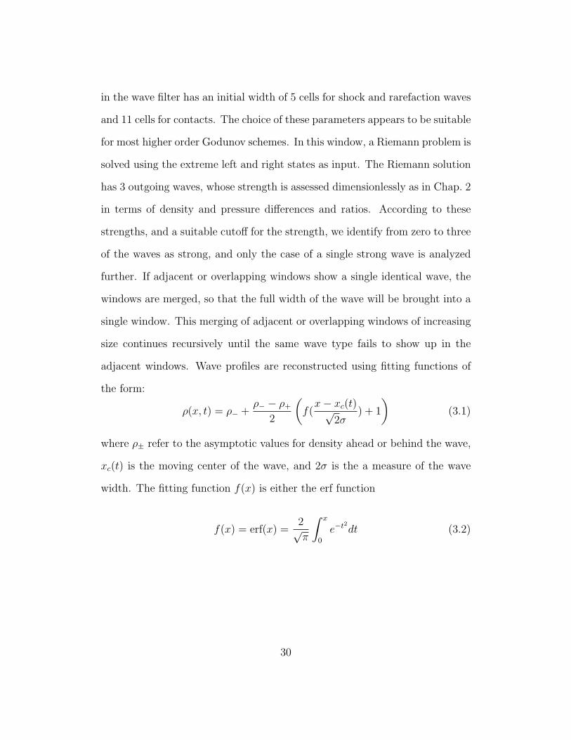
adjacent windows. Wave profiles are reconstructed using fitting functions of
the form:
ρ(x, t) = ρ− +ρ− − ρ+
2
(f(
x − xc(t)√2σ
) + 1
)(3.1)
where ρ± refer to the asymptotic values for density ahead or behind the wave,
xc(t) is the moving center of the wave, and 2σ is the a measure of the wave
width. The fitting function f(x) is either the erf function
f(x) = erf(x) =2√π
∫ x
0
e−t2dt (3.2)
30
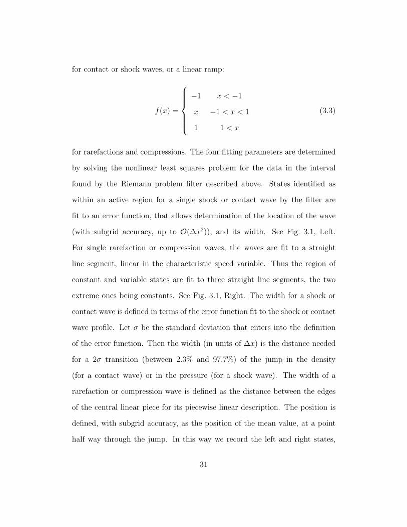
for contact or shock waves, or a linear ramp:
f(x) =
⎧⎪⎪⎪⎪⎨⎪⎪⎪⎪⎩
−1
x
1
x < −1
−1 < x < 1
1 < x
(3.3)
for rarefactions and compressions. The four fitting parameters are determined
by solving the nonlinear least squares problem for the data in the interval
found by the Riemann problem filter described above. States identified as
within an active region for a single shock or contact wave by the filter are
fit to an error function, that allows determination of the location of the wave
(with subgrid accuracy, up to O(∆x2)), and its width. See Fig. 3.1, Left.
For single rarefaction or compression waves, the waves are fit to a straight
line segment, linear in the characteristic speed variable. Thus the region of
constant and variable states are fit to three straight line segments, the two
extreme ones being constants. See Fig. 3.1, Right. The width for a shock or
contact wave is defined in terms of the error function fit to the shock or contact
wave profile. Let σ be the standard deviation that enters into the definition
of the error function. Then the width (in units of ∆x) is the distance needed
for a 2σ transition (between 2.3% and 97.7%) of the jump in the density
(for a contact wave) or in the pressure (for a shock wave). The width of a
rarefaction or compression wave is defined as the distance between the edges
of the central linear piece for its piecewise linear description. The position is
defined, with subgrid accuracy, as the position of the mean value, at a point
half way through the jump. In this way we record the left and right states,
31

wave position (and hence speed) and wave width. These quantities are not
independent, as the speeds and jumps are connected by the Rankine-Hugoniot
jump relations. They are sufficient to fully characterize the numerical incoming
waves. The location where the linear fit attains the far field state is marked
as the edge of the wave, and its width is the distance between its two edges.
Finally, the filter regards any shock like wave that is ”too wide” in mesh units
to be a compression wave.
The wave filter is the fundamental diagnostic tool that identifies indi-
vidual waves, here within the solution of a numerical Riemann problem and
in Sec. 5.1 within the solution of a complex wave interaction problem. We
note immediately a limitation of the methodology, at least as presently de-
veloped. The definition of the wave filters assume that the individual waves
in the Riemann problem have separated. For sufficiently coarse grids in the
wave interaction problem of Sec. 5.1, the waves will enter into new interactions
before clearly separating as they leave an earlier interaction. A second, and re-
lated limitation concerns the relaxation of the left and right states at the edge
of a wave to their far field values, an issue studied in Sec. 3.2. If a subsequent
interaction occurs before this relaxation is complete, the associated errors will
be “frozen” into the input and output of this later interaction. We will assess
this issue in Sec. 5.1.
A statistical distribution of numerical incoming waves and starting states
determines the SNRP. Its solution gives the output waves, each of which gen-
erate the same type of data Thus we define the SNRP as a statistical (non-
deterministic) mapping from a statistical input wave description to a statistical
32
output wave description.
Figure 3.1: Schematic diagram illustrating the operation of a wave filter. Left:computational data (squares) are fit to an error function. The error functiondepends on four parameters, a position, a width, and two asymptotic values.These determine the wave position, width and height, with subgrid accuracy.Right: a piecewise linear construction is fit to the rarefaction or compressionwave data.
The statistics of the SNRP mapping function arise from grid errors, and
from the random placement of a traveling wave relative to the centers of the
finite difference lattice. Our first objective in this section is to compare and
contrast the SRP and the SNRP. Our second objective is to build up a library
of statistical input-output relations that will include all Riemann problems to
be encountered in Sec. 5.1. This library will be used to predict results for
the multiwave error and uncertainty analysis based on a multi-path scattering
formula.
33
3.2 Isolated Waves
We start with the analysis of the ensemble mean width of a single (non-
interacting) shock wave. Fig. 3.2 (left) shows the expected narrow and time
independent (∼ 2∆x) shock width. Among the several factors contributing to
wave strength and speed errors, we mention the finite accuracy of the Riemann
solution root solver, or some approximate Riemann solver and the numerical
(finite difference) nature of the solution. The latter arises in two ways, the
relaxation to a constant ambient state and the finite rate of convergence under
mesh refinement, both applicable on the post shock or up stream side of the
shock wave. The equivalence of these two effects can be seen from the self
similar nature of the Riemann solution, which implies that the fixed mesh,
large time limit, with evaluation of the ambient state at a large separation
from the traveling wave is equivalent to a fixed separation at a fixed time,
considered as a mesh refinement problem.
According to the theory of traveling waves for the viscous Riemann prob-
lem [36], considered as a model for numerically generated traveling waves, we
expect an exponential approach of the numerical shock profile to its limiting
values at x = ±∞. Depending on the numerical scheme this approach may be
oscillatory. For higher order flux or slope limited methods there is a trade-off
between the oscillations and the wave width, as the oscillations are reduced
through increase of the first order (diffusive) aspect of the algorithm, while the
wave width is reduced through decrease in this diffusiveness. The error occurs
on the upwind side of the shock, while the downwind states converge to their
far field values within a few mesh blocks. In Fig. 3.2 (right), we measure the
34
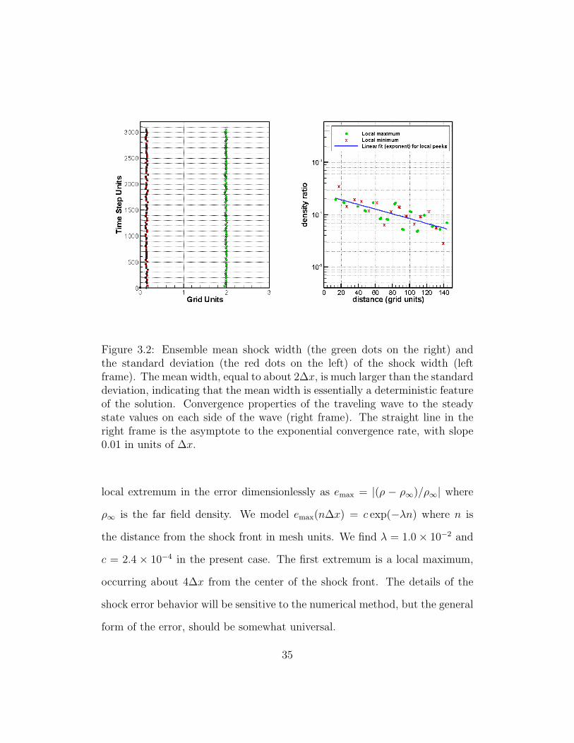
Figure 3.2: Ensemble mean shock width (the green dots on the right) andthe standard deviation (the red dots on the left) of the shock width (leftframe). The mean width, equal to about 2∆x, is much larger than the standarddeviation, indicating that the mean width is essentially a deterministic featureof the solution. Convergence properties of the traveling wave to the steadystate values on each side of the wave (right frame). The straight line in theright frame is the asymptote to the exponential convergence rate, with slope0.01 in units of ∆x.
local extremum in the error dimensionlessly as emax = |(ρ − ρ∞)/ρ∞| where
ρ∞ is the far field density. We model emax(n∆x) = c exp(−λn) where n is
the distance from the shock front in mesh units. We find λ = 1.0 × 10⁻² and
c = 2.4 × 10⁻⁴ in the present case. The first extremum is a local maximum,
occurring about 4∆x from the center of the shock front. The details of the
shock error behavior will be sensitive to the numerical method, but the general
form of the error, should be somewhat universal.
35
Fig. 3.3 (left) shows the larger contact width wc ∼ cct1/3 growing from 2
to 30 cells with a rate asymptotically proportional to t1/3. Similar asymptotics
have been observed by Harten [23] for an ENO scheme. The rate t1/3 results
from the second order accuracy of the method used here. The coefficient cc of
the growth law is sensitive to the ambient Mach number M of the flow, and
more specifically to a transport CFL number θ = |v|/(|v| + c) = M/(M + 1),
assuming that the algorithm has a time step set by the CFL limit ∆t =
∆x/(|v|+ c). Here c = max{cl, cr} is the maximum of the left and right state
sound speeds cl and cr respectively, and v is the fluid velocity. The contact
advances a fraction θ of one mesh cell in a single time step. For θ = 0 or θ = 1,
the contact does not move in its position relative to the grid lines and cc = 0.0.
This value (cc = 0.0) is applicable for a very narrow range of theta. For most
of the range of θ, the numerical diffusion is sensitive to the direction of mixing.
For θ < 0.5 and the flow from high density to low, the numerical mixing is
that of heavy fluid into light. We call this the step down problem. For the step
down problem, the ensemble mean contact width is shown in Fig. 3.3 (left).
For most θ values, we find cc ∼ 1,
The reverse, called the step up problem, flows from light to heavy fluid.
It mixes small amounts of light fluid into heavy, an effect less noticeable in
terms of the diffusion width, especially for large density contrasts. For step up
flow, we find wc ∼ min{5, cct1/3}. See Fig. 3.3, in which the mean wave width
grows firstly following wc ∼ cct1/3, then stops around wc ∼ 5. As a partial
explanation of this difference between the step down and step up problems, we
note that the spreading is primarily associated with the up stream side of the
36

Figure 3.3: Ensemble mean contact width for isolated noninteracting waves.Because the width is entirely grid related, we record width in units of ∆x andtime in units of the number of time steps. The standard deviations are alsoplotted as the red points to the extreme left in each frame. Left (step down):we observe an increase from 2 cells to 30 over 104 steps and an asymptoticgrowth rate cct
1/3, where cc ∼ 1 depends on the flow Mach number. Thestraight line in the left frame is the asymptote to the contact width, withslope 3. Right (step up): We observe a bound on the contact width.
contact, and that continued spreading (the t1/3 asymptotic) depends on the
up stream flow being subsonic. The higher sound speed in the light fluid gives
a supersonic upstream state for the step up problem but not for the step down
problem, for the flow parameters considered here. These properties appear
to be sensitive to the details of the numerical algorithm, and specifically to
the form of the limiter employed. We have used a MUSCL algorithm. The
general form of the error model and even some of its specific features, such as
shock wave widths should be solver independent. The degree of recalibration
of the model presented here for other solvers, is an important question which
37

is beyond the scope of this study.
For some aspects of the solution error, the probabilistic error formalism
is more general than is required. When the standard deviation of the error
is much smaller than the mean error (when the coefficient of variation, their
ratio, is close to zero), then the error is essentially deterministic, and the
probabilistic formulation is unnecessary. The standard deviation of the width,
shown to the left in each frame of Fig. 3.3, is significantly smaller than the mean
width, indicating that the wave width is essentially a deterministic feature of
the numerical solution. The wave position errors have a statistical aspect,
especially in their transient behavior.
3.3 Interactions with Contact Waves
We study wave strength, speed and position errors after a wave interac-
tion. Note that the SNRP errors considered so far are not the same as errors
in the SRP.
We represent the wave properties as a quadruple
wak = (ωa
k , λak, s
ak, p
ak) , (3.4)
where ω, as in Chap. 2, is a wave strength, λ is a wave width(A or P ), s is a
wave speed error, and p is a position error. Also a = i for input and a = o for
output. The units for wave strengths are dimensionless. We measure the wave
width in units of mesh spacing with contacts having either a t1/3 or bounded
time dependence. Thus we interpret λi2 as the input contact wave width at the
38
time of interaction (no time dependence) and either λo2t
1/3 or λo2 as the output
contact wave width, depending on the up stream Mach number. Here t is the
elapsed time since the interaction, expressed in time step units. As the shock
width is deterministic and time independent, it is not needed as an input or an
output variable. The wave speed error s is specified dimensionlessly as a ratio
(relative to the exact speed value), and occurs only as an output variable. It
refers to a far field (large time) value, after the waves are well separated. This
large time asymptotic speed error is very small, and will not be considered
further. Near field (near interaction) state errors are given by an oscillatory
decaying exponential, approaching the far field value. The exponent, or decay
rate, characterizes this approach in a simple overall manner. See Sec. 3.2.
Wave position errors are specified in grid units, after an isolated transient
period.
The input multi-index J = (j1, j2, j3) now has three components while
the output multi index has six (to reflect the dependence on three position
errors pok). Using J , we define the power expressions
wi,J = (ωi1)
j1(ωi2)
j2(λi2)
j3 .
For the three interactions we will study, the input wave width (λi2)
j3 is not
used, i.e. modeled as being zero. With these conventions, Eq. (2.1) also de-
scribes the model for the SNRP, but now each coefficient αk,J is also a random
variable, reflecting randomness in the numerical solution algorithm, such as
the dependence of the solution on the sub-grid location of the interaction point
39
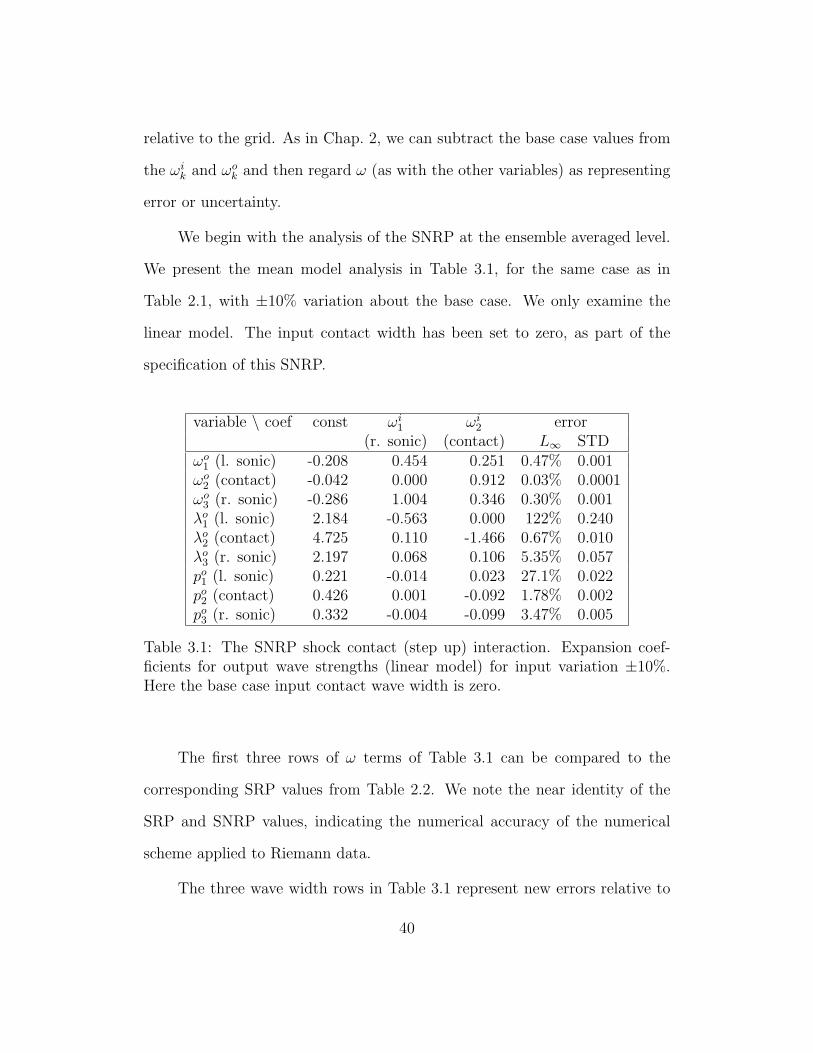
relative to the grid. As in Chap. 2, we can subtract the base case values from
the ωik and ωo
k and then regard ω (as with the other variables) as representing
error or uncertainty.
We begin with the analysis of the SNRP at the ensemble averaged level.
We present the mean model analysis in Table 3.1, for the same case as in
Table 2.1, with ±10% variation about the base case. We only examine the
linear model. The input contact width has been set to zero, as part of the
specification of this SNRP.
variable \ coef const ωi1 ωi
2 error(r. sonic) (contact) L∞ STD
ωo1 (l. sonic) -0.208 0.454 0.251 0.47% 0.001
ωo2 (contact) -0.042 0.000 0.912 0.03% 0.0001
ωo3 (r. sonic) -0.286 1.004 0.346 0.30% 0.001
λo1 (l. sonic) 2.184 -0.563 0.000 122% 0.240
λo2 (contact) 4.725 0.110 -1.466 0.67% 0.010
λo3 (r. sonic) 2.197 0.068 0.106 5.35% 0.057
po1 (l. sonic) 0.221 -0.014 0.023 27.1% 0.022
po2 (contact) 0.426 0.001 -0.092 1.78% 0.002
po3 (r. sonic) 0.332 -0.004 -0.099 3.47% 0.005
Table 3.1: The SNRP shock contact (step up) interaction. Expansion coef-ficients for output wave strengths (linear model) for input variation ±10%.Here the base case input contact wave width is zero.
The first three rows of ω terms of Table 3.1 can be compared to the
corresponding SRP values from Table 2.2. We note the near identity of the
SRP and SNRP values, indicating the numerical accuracy of the numerical
scheme applied to Riemann data.
The three wave width rows in Table 3.1 represent new errors relative to
40

the SRP. The large sup norm error for the λo1 results from a few outliers. The
standard deviation for this quantity is about 10% of the mean value, indicating
that the error model is (on the whole) satisfactory, and that the shock wave
widths are not fluctuating greatly. The outliers are mainly associated with
time steps and realizations for which the (narrow) reflected shock has at most
one internal mesh point. For these cases, our wave filter tool for assessing
the numerical shock width and position is not effective, so the outliers can be
viewed as a breakdown of the diagnosis methodology.
The shock speed errors are nearly zero (to 5 digit accuracy in relative
shock speed errors) after the interacting waves separate; these errors are not
presented in Table 3.1. Consistent with the convergence properties of the
traveling wave to its left and right states shown in Fig. 3.2, accurate determi-
nation of shock speed requires well separated waves, and thus a highly resolved
calculation.
We now consider the wave position errors. This would be equivalent to
studying timing errors (for example in wave arrival), since position errors are
the integral of the velocity errors. Fig. 3.4 shows the position errors as a
function of time. The fact that the position errors reach a steady nonzero
asymptotic value is equivalent to the fact that the speed errors tend to zero,
with a nonzero time averaged value. The initial transient error will be signif-
icant when we consider errors in under resolved simulations. Following this
transient, the position error is constant, reflecting convergence of the wave
speed to its exact value. The errors in the wave position rows of Table 3.1
present this constant error. All position errors are sub-grid. The standard
41
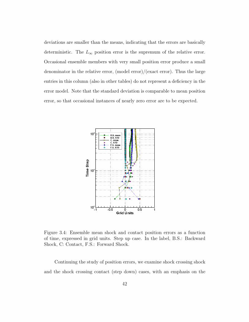
deviations are smaller than the means, indicating that the errors are basically
deterministic. The L∞ position error is the supremum of the relative error.
Occasional ensemble members with very small position error produce a small
denominator in the relative error, (model error)/(exact error). Thus the large
entries in this column (also in other tables) do not represent a deficiency in the
error model. Note that the standard deviation is comparable to mean position
error, so that occasional instances of nearly zero error are to be expected.
Figure 3.4: Ensemble mean shock and contact position errors as a functionof time, expressed in grid units. Step up case. In the label, B.S.: BackwardShock, C: Contact, F.S.: Forward Shock.
Continuing the study of position errors, we examine shock crossing shock
and the shock crossing contact (step down) cases, with an emphasis on the
42

transient error. Fig. 3.5 shows that the transient error is significant, on the
order of the mesh spacing, and the standard deviation is also significant, in
contrast to the steady or large time asymptotics emphasized in Fig. 3.4. These
transient errors are important for underresolved simulations.
Figure 3.5: Ensemble mean shock and contact position errors as a functionof time, expressed in grid units. To emphasize the transient errors, a smallernumber of time steps are shown. Left: shock crossing shock case. Right: shockcrossing contact (step down) case.
3.4 Shock Crossing Shock Interactions
Here we study the reflection of the shock off a wall, a special case of a
shock crossing shock interaction. We can ignore the shock wave width para-
meters, as these are narrow and deterministic. We only consider one output
wave position error, po1 as presented in Table 3.2. The shock wave strength
errors (the far field, large separation errors) are small.
43

variable \ coef const ωi1 error
(r. sonic) L∞ STDωo
1 (l. sonic) -0.002 0.716 0.014% 0.000032λo
1 (l. sonic) 2.291 -0.422 7.923% 0.062po
1 (l. sonic) 0.060 -0.039 5065% 0.009ωo
2 (contact) 0.057 0.0003 24.4% 0.005λo
2 (contact) 5.9 50% 0.7
Table 3.2: The SNRP defined by the crossing of two shocks. Expansion coef-ficients for output wave strengths, widths and position errors (linear model)for input variation ±10%.
The contact mode contributes an error, well known as shock wall heating.
The exact solution doesn’t have this error in this mode for a wall reflection.
The error is due to the entropy, temperature and density variables from entropy
errors made during the shock interaction process. Since entropy can only
increase these errors do not cancel. Because the solution algorithm conserves
mass locally, we expect the spatial integral of the density errors to cancel
approximately. Since the velocity of the fluid at the wall is zero, these errors
remain permanently attached to the wall. We do not have a theoretical model
for the form of these errors; therefore, our fitting of the errors will be less
precise than those discussed elsewhere in this paper. We define the ”wall error
width” to be the distance to the wall in mesh units of the furthest location
for which the density error is at least twice the background noise in the post
shock region, or about 1% of the base case density. This width is about 6∆x.
The wave strength error is defined dimensionlessly as the L1 error in density,
divided by ρ0∆x, where ρ0 is the base case post shock density after the wall
reflection.
44

3.5 The Contact Reshock Interactions
Figure 3.6: Problem 3: Contact-shock (step down).
After reflection from the wall, the transmitted lead shock wave re-crosses
the deflected contact, see Fig. 3.6. This is a step down interaction. We have
one input and one output wave width parameter, both are for the contact.
According to the analysis of Sec. 3.2, the contact width is modeled as cct1/3
and this formula is accurate after some 50 time steps. In Table 3.3, entry
λo2 = cc. The rarefaction width has the form constant + rate × time. We find
very small errors in this rate, not tabulated here. The entry λo3 refers to the
constant, which gives an offset for the centering of the rarefaction wave.
45
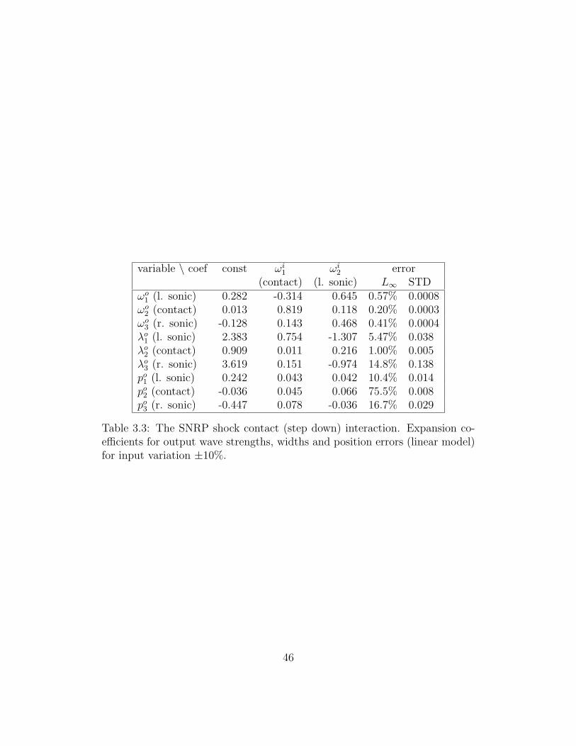
variable \ coef const ωi1 ωi
2 error(contact) (l. sonic) L∞ STD
ωo1 (l. sonic) 0.282 -0.314 0.645 0.57% 0.0008
ωo2 (contact) 0.013 0.819 0.118 0.20% 0.0003
ωo3 (r. sonic) -0.128 0.143 0.468 0.41% 0.0004
λo1 (l. sonic) 2.383 0.754 -1.307 5.47% 0.038
λo2 (contact) 0.909 0.011 0.216 1.00% 0.005
λo3 (r. sonic) 3.619 0.151 -0.974 14.8% 0.138
po1 (l. sonic) 0.242 0.043 0.042 10.4% 0.014
po2 (contact) -0.036 0.045 0.066 75.5% 0.008
po3 (r. sonic) -0.447 0.078 -0.036 16.7% 0.029
Table 3.3: The SNRP shock contact (step down) interaction. Expansion co-efficients for output wave strengths, widths and position errors (linear model)for input variation ±10%.
46

Chapter 4
The Statistical Numerical Riemann Problems
for Spherical Flows
We consider the interaction of a spherically symmetric shock wave with a
contact located near the origin. The interactions are illustrated by the space
time contour plots of the density, shown in Fig. 4.1 (left). In Fig. 4.1 (right),
we show the type and location of the waves, as determined by the wave filter
analysis program. Both figures show results for the base case. The build up
of complex wave patterns is evident.
We consider statistical numerical Riemann problems (SNRP) in spherical
geometry. Because of the possible width of the input waves, the problem and
its solution are not strictly scale invariant. Moreover, scale invariance is lost
through the length scale introduced by the radius at the time of interaction.
We are then considering a generalization of the spherically symmetric Riemann
problem.
The statistics of the SNRP mapping function arise from grid errors, and
from the random placement of a traveling wave relative to the centers of the
47
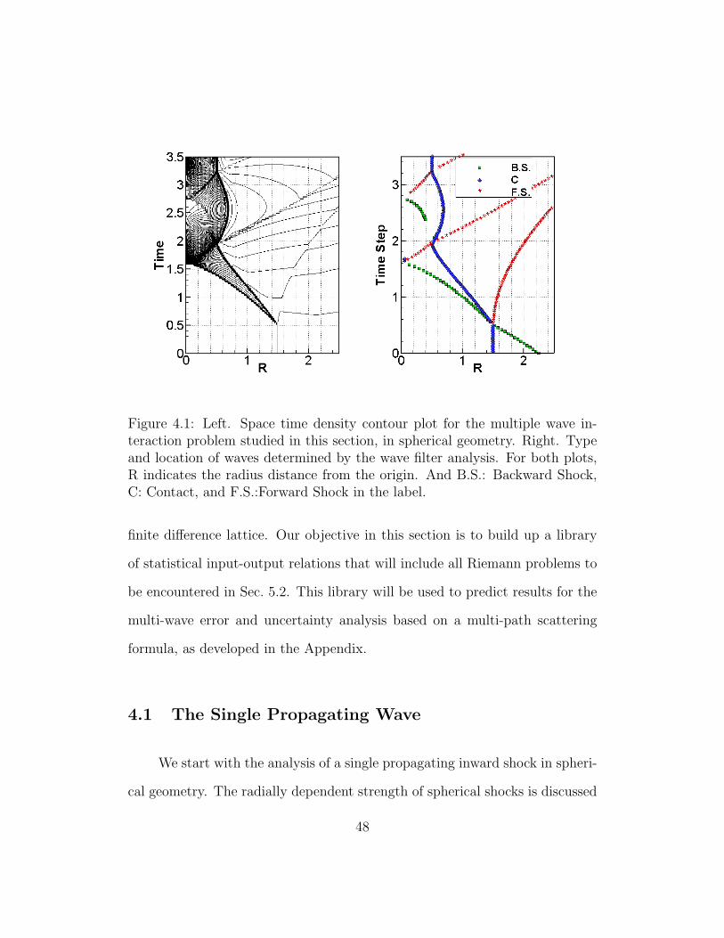
Figure 4.1: Left. Space time density contour plot for the multiple wave in-teraction problem studied in this section, in spherical geometry. Right. Typeand location of waves determined by the wave filter analysis. For both plots,R indicates the radius distance from the origin. And B.S.: Backward Shock,C: Contact, and F.S.:Forward Shock in the label.
finite difference lattice. Our objective in this section is to build up a library
of statistical input-output relations that will include all Riemann problems to
be encountered in Sec. 5.2. This library will be used to predict results for the
multi-wave error and uncertainty analysis based on a multi-path scattering
formula, as developed in the Appendix.
4.1 The Single Propagating Wave
We start with the analysis of a single propagating inward shock in spheri-
cal geometry. The radially dependent strength of spherical shocks is discussed
48
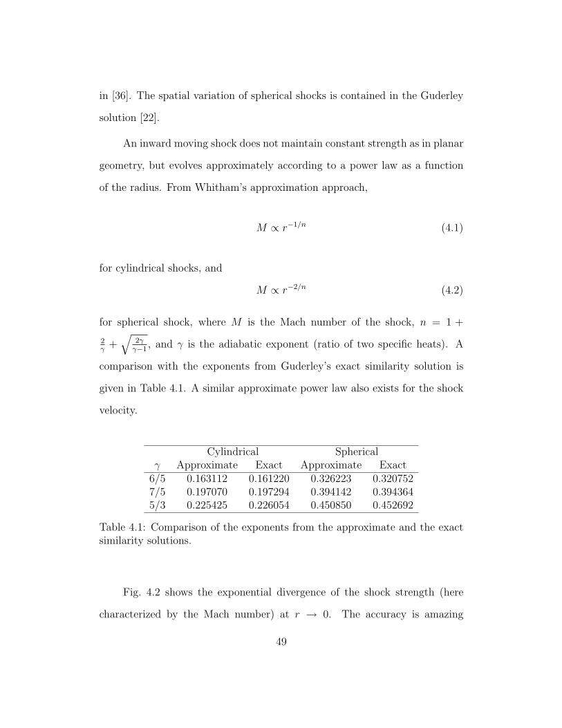
in [36]. The spatial variation of spherical shocks is contained in the Guderley
solution [22].
An inward moving shock does not maintain constant strength as in planar
geometry, but evolves approximately according to a power law as a function
of the radius. From Whitham’s approximation approach,
M ∝ r−1/n (4.1)
for cylindrical shocks, and
M ∝ r−2/n (4.2)
for spherical shock, where M is the Mach number of the shock, n = 1 +
2γ
+√
2γγ−1
, and γ is the adiabatic exponent (ratio of two specific heats). A
comparison with the exponents from Guderley’s exact similarity solution is
given in Table 4.1. A similar approximate power law also exists for the shock
velocity.
Cylindrical Sphericalγ Approximate Exact Approximate Exact
6/5 0.163112 0.161220 0.326223 0.3207527/5 0.197070 0.197294 0.394142 0.3943645/3 0.225425 0.226054 0.450850 0.452692
Table 4.1: Comparison of the exponents from the approximate and the exactsimilarity solutions.
Fig. 4.2 shows the exponential divergence of the shock strength (here
characterized by the Mach number) at r → 0. The accuracy is amazing
49
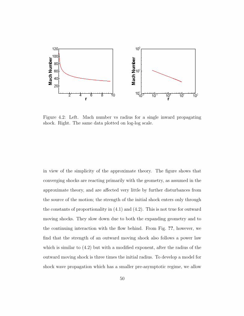
Figure 4.2: Left. Mach number vs radius for a single inward propagatingshock. Right. The same data plotted on log-log scale.
in view of the simplicity of the approximate theory. The figure shows that
converging shocks are reacting primarily with the geometry, as assumed in the
approximate theory, and are affected very little by further disturbances from
the source of the motion; the strength of the initial shock enters only through
the constants of proportionality in (4.1) and (4.2). This is not true for outward
moving shocks. They slow down due to both the expanding geometry and to
the continuing interaction with the flow behind. From Fig. ??, however, we
find that the strength of an outward moving shock also follows a power law
which is similar to (4.2) but with a modified exponent, after the radius of the
outward moving shock is three times the initial radius. To develop a model for
shock wave propagation which has a smaller pre-asymptotic regime, we allow
50
two distinct exponents,
M ∝
⎧⎪⎨⎪⎩
ra1
ra2
r0 ≤ r ≤ 3r0
r ≥ 3r0.(4.3)
Here we choose a1 = −0.4, a2 = −1.0 for γ = 1.67, and r0 is the initial shock
radius.
Figure 4.3: Left. Mach number vs radius for a single outgoing propagatingshock. Right. The same data plotted on log-log scale.
We also study a single propagating contact. Fig. 4.4 shows that the
contact width grows from 2 to 5 cells with an asymptotically rate wc ∼ cct1/2.
For some aspects of the solution error, the probabilistic error formalism is more
general than is required. The standard deviation of the width, as shown to
the left in the frame of Fig. 4.4, is significantly smaller than the mean width,
indicating that the wave width is essentially a deterministic feature of the
numerical solution.
51

Figure 4.4: Ensemble mean contact width for single propagating contact. Werecord width in units of ∆x. The standard deviations are also plotted. andare the points to the extreme left in the frame.
4.2 The Shock Contact Interaction
We study the wave strength, speed, width and position errors after a
wave interaction. Similar to Eq. 3.4, we represent the wave properties as a
five tuple
wak = (ωa
k , δak , λ
ak, s
ak, p
ak) , (4.4)
where ω is a wave strength, δ is an error in the wave strength, λ is a wave
width, s is a wave speed error, and p is a position error. Also a = i denotes
input and a = o signifies output. We choose dimensionless variables to measure
wave strengths; the Atwood number A = (ρ2 − ρ1)/(ρ2 + ρ1) to measure the
contact strength, and the Mach number M defined as the ratio of the shock
52

speed to the ahead state sound speed, in the frame of a stationary ahead
state, for the shocks. We measure the wave widths in units of mesh spacing.
The wave position errors are specified in grid units, after an initial transient
period. Within this formulation, we can describe the output wave errors by an
expression multi-linear (and eventually linear) in the two input wave strengths,
i.e. linear in each of the two input wave strengths.
We begin with the analysis of the initial shock contact SNRP at the
ensemble averaged level. We present the linear model coefficients in Table 4.2,
with ±10% variation for the initial contact strength and ±5% variation for the
initial shock strength (consistent with ±10% variation in pressure ratio as used
in the planar study) about the base case. According to the analysis of Sec. 4.1,
the strength of this initial inward shock is not constant, and is increasing as it
moves toward the origin. We use the power law M = Cr−2/n to estimate the
initial shock strength at the interaction time and use this quantity represented
by the variable C as the input shock strength in the modeling. The input
contact width has been set to zero, as part of the specification of this SNRP.
To read Table 4.2, we note that the first (ωo1) row (labeled in the table
as wo1 (l. sonic)) lists coefficients α1,J for J = (0, 0), J = (1, 0), etc. These
coefficients are determined by a least squares algorithm that minimizes the
expected, or mean error over the ensemble, in comparing the linear predic-
tions to the exact solution of the Riemann problem. The last two columns
describe errors in the model (2.1). The presence of outliers was monitored and
the ensemble L∞ norm determined (results not tabulated); occasional outliers
indicate non Gaussian statistics. The model error is defined as (predicted - ex-
53

act) where exact is the result of the simulation and predicted is the value given
by the finite polynomial (linear) model (2.1). The column STD is the standard
deviation of (predicted - exact). Note that the STD errors, as defined, are di-
mensionful. To aid in interpreting the error magnitudes, we present in a final
column (labeled STD/ωo) the standard deviation of the error in the model
divided by the mean value of the variable predicted. This column represents
a fractional (dimensionless) error in the model.
According to the analysis of Sec. 4.1, the strength of the output inward
moving shock is modeled as Cr−2/n. This formula is accurate after some time,
and the Table 4.2 entry is ωo1 = C in this formula. We form a linear model for
this constant in this expression in Table 4.2. We find very small errors in the
exponent, not tabulated here. We developed a model (4.3) for the strength of
the output outward moving shock in Sec. 4.1. Here in our study, we are only
concerned with the first formula in (4.3). The entry ωo3 in the table represents
the coefficient multiplying the power term.
The three variable (λ) rows in Table 4.2 represent wave width errors.
The standard deviation for this quantity is about 10% of the mean value,
indicating that the error model is (on the whole) satisfactory, and that the
shock wave widths are not (mostly) fluctuating greatly. The inward moving
shock width decreased about 10% relative to the wave width at the interaction
time, while the outward moving shock width increased about 10%. See Fig. 4.5,
left frame. The contact width is modeled as cct1/5 where both the width and t
are expressed in mesh units. The Table 4.2 entry λo2 = cc in this formula. We
form a linear model for this constant in this expression in Table 4.2.
54

Figure 4.5: Left: ensemble mean inward/outward moving shock and contactwidths after a shock contact interaction. Right: ensemble mean shock andcontact position errors as a function of time, expressed in grid units. Theassociated standard deviations are extremely small, not shown in the plots.In the legend, C. denotes the contact while I.S. and O.S. are the inward andoutward moving shocks.
We also study the wave position errors. Fig. 4.5, right frame, shows the
position errors as a function of time. The entries in the wave position rows
of Table 4.2 present those errors, given in mesh units. All position errors are
subgrid. The standard deviations are smaller than the means, indicating that
the errors are basically deterministic.
All solution errors are sensitive to the grid spacing, taken to be 100
computational cells in Table 4.2-4.4. This sensitivity is not extreme. For
example, if the 100 cell model is used to analyze the 500 cell data, the model
errors (STD) approximately double, but remain small.
55
4.3 Shock Reflection at the Origin
Here we study the reflection of the shock off the origin. According to the
analysis of Sec. 4.1, the input inward moving shock has infinite strength at the
origin. We used the strength at the radius r = 1 as the initial state and the
input shock strength in the modeling process. We study the wave strength,
wave strength errors, wave width and wave position errors. See Table 4.3.
We found that the Mach number of the outward moving shock (reflected
shock) was essentially independent of the input variation in Mach number. To
explain this phenomena, we recall that the ambient state ahead of the outward
moving reflected shock is an incoming continuously variable flow. The sound
speed ahead of this flow is affine linearly dependent on the strength of the
incoming shock wave, as is the shock speed of the reflected outward moving
shock wave. Thus the outward moving Mach number, as a ratio of two quan-
tities varying affine linearly with the incoming shock strength, has a fractional
linear form in the incoming wave strength. A simple calculation shows that
the variation in the outward moving shock Mach number Mo contains the fac-
tor (1−Mo) and since Mo ≈ 1.2, this small factor suppressed variation in Mo
as a function of Mi, the Mach number of the incoming shock. Thus the Mach
number is not a good measure for the outward moving shock strength. We
choose the pressure behind the reflected shock instead as ωo1 in Table 4.3. The
pressure also follows the power law. The large entries in this row result from
the fact that the (dimensional) pressure (ωo1) is much larger in pressure units
than the Mach number (ωi1).
56
4.4 The Contact Reshock Interaction
After reflection from the origin, the transmitted lead shock wave re-
crosses the deflected contact. The outgoing waves from this interaction consist
of a rarefaction wave propagating toward the origin, a contact and a shock
propagating outward. The region inside of the outward propagating shock, on
both sides of the contact is not piecewise constant, but contains an inward
propagating compression, which eventually breaks to form an inward moving
shock, reaching the origin at interaction 4. This inward moving compression
is generated from the geometrically caused weakening of the outward moving
shock, and is a well recognized aspect of spherical shock wave dynamics. The
shock and the rarefaction interact, and eventually the rarefaction disappears
in this interaction. Here we only follow the waves through the output of in-
teraction 3, and thus avoid much of this interaction. Specifically, we focus on
the inward moving rarefaction and not the inward moving shock. We study
the wave strength, wave strength errors, wave width and wave position errors
resulting from interaction 3. See Table 4.4.
According to the analysis of Sec. 4.1, this is a step down interaction and
the contact width is modeled as cct1/5 where both the width and t are expressed
in mesh units. We form a linear model for the coefficient cc in this expression
in Table 4.4. The rarefaction width has the form constant + rate × time. The
entry λo1 refers to the constant, which gives an offset for the centering of the
rarefaction wave. This entry is expressed in mesh units.
57
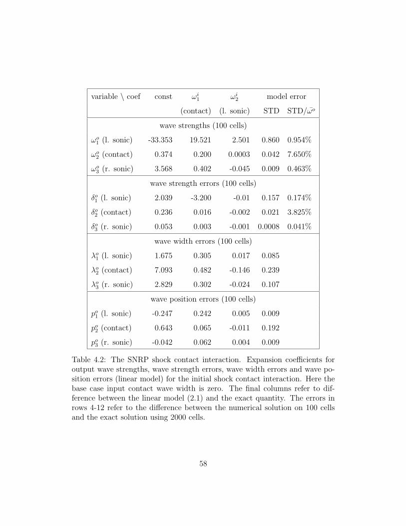
variable \ coef const ωi1 ωi
2 model error
(contact) (l. sonic) STD STD/ωo
wave strengths (100 cells)
ωo1 (l. sonic) -33.353 19.521 2.501 0.860 0.954%
ωo2 (contact) 0.374 0.200 0.0003 0.042 7.650%
ωo3 (r. sonic) 3.568 0.402 -0.045 0.009 0.463%
wave strength errors (100 cells)
δo1 (l. sonic) 2.039 -3.200 -0.01 0.157 0.174%
δo2 (contact) 0.236 0.016 -0.002 0.021 3.825%
δo3 (r. sonic) 0.053 0.003 -0.001 0.0008 0.041%
wave width errors (100 cells)
λo1 (l. sonic) 1.675 0.305 0.017 0.085
λo2 (contact) 7.093 0.482 -0.146 0.239
λo3 (r. sonic) 2.829 0.302 -0.024 0.107
wave position errors (100 cells)
po1 (l. sonic) -0.247 0.242 0.005 0.009
po2 (contact) 0.643 0.065 -0.011 0.192
po3 (r. sonic) -0.042 0.062 0.004 0.009
Table 4.2: The SNRP shock contact interaction. Expansion coefficients foroutput wave strengths, wave strength errors, wave width errors and wave po-sition errors (linear model) for the initial shock contact interaction. Here thebase case input contact wave width is zero. The final columns refer to dif-ference between the linear model (2.1) and the exact quantity. The errors inrows 4-12 refer to the difference between the numerical solution on 100 cellsand the exact solution using 2000 cells.
58

variable \ coef const ωi1 model error
(l. sonic) STD STD/ωo
ωo1 (r. sonic) -242.394 5.606 1.137 0.468%
δo1 (r. sonic) -3.27 0.031 0.112 0.045%
λo1 (r. sonic) 1.221 0.018 0.099
po1 (r. sonic) 0.474 0.001 0.012
Table 4.3: The SNRP defined by the shock reflection at the origin. Expansioncoefficients for output wave strengths, wave strength errors, wave width errorsand wave position errors (linear model) for input variation ±10%.
59

variable \ coef const ωi1 ωi
2 model error
(r. sonic) (contact) STD STD/ωo
wave strengths (100 cells)
ωo1 (l. sonic) 0.097 -0.108 0.436 0.031 13.305%
ωo2 (contact) 0.103 -0.192 1.168 0.007 1.116%
ωo3 (r. sonic) 0.988 0.195 -0.225 0.003 0.262%
wave strength errors (100 cells)
δo1 (l. sonic) -0.291 0.161 -0.468 0.017 7.296%
δo2 (contact) -0.067 0.142 -0.125 0.006 0.957%
δo3 (r. sonic) -0.030 0.107 -0.0004 0.001 0.087%
wave width errors (100 cells)
λo1 (l. sonic) 9.776 -6.372 5.091 0.484
λo2 (contact) 1.903 0.156 -0.677 0.534
λo3 (r. sonic) 4.088 -1.401 1.549 0.168
wave position errors (100 cells)
po1 (l. sonic) 4.782 -3.602 2.372 0.379
po2 (contact) -0.453 0.409 -0.054 0.177
po3 (r. sonic) -0.199 -0.685 3.213 0.052
Table 4.4: The SNRP contact reshock interaction. Expansion coefficientsfor output wave strengths, wave strength errors, wave width errors and waveposition errors (linear model).
60
Chapter 5
Composite Shock Interaction Problems
5.1 Composite Shock Interaction Problems In Planar
Flows
Here we introduce a formula for combining the wave interaction errors
defined in Chap. 2 and 3 for isolated Riemann problems, to yield the error
for arbitrary points in the colution of the complex wave interaction problem.
The formula is validated for fully resolved simulations and it is shown to be
partially correct and partially incorrect for under resolved simulations.
5.1.1 A Multipath Integral for a Nonlinear Multiscat-
tering Problem
We begin with a formula expressing the error in a given Riemann problem
R0 as multinomial expansion associated with initial waves and errors located
inside its domain of dependence. For a 1D shock wave interaction problem,
think of the solution as being primarily composed of localized waves, interact-
61
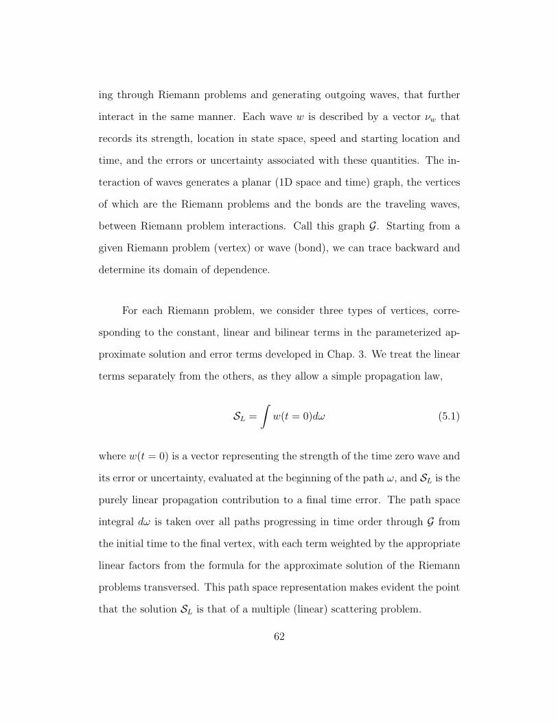
ing through Riemann problems and generating outgoing waves, that further
interact in the same manner. Each wave w is described by a vector νw that
records its strength, location in state space, speed and starting location and
time, and the errors or uncertainty associated with these quantities. The in-
teraction of waves generates a planar (1D space and time) graph, the vertices
of which are the Riemann problems and the bonds are the traveling waves,
between Riemann problem interactions. Call this graph G. Starting from a
given Riemann problem (vertex) or wave (bond), we can trace backward and
determine its domain of dependence.
For each Riemann problem, we consider three types of vertices, corre-
sponding to the constant, linear and bilinear terms in the parameterized ap-
proximate solution and error terms developed in Chap. 3. We treat the linear
terms separately from the others, as they allow a simple propagation law,
SL =
∫w(t = 0)dω (5.1)
where w(t = 0) is a vector representing the strength of the time zero wave and
its error or uncertainty, evaluated at the beginning of the path ω, and SL is the
purely linear propagation contribution to a final time error. The path space
integral dω is taken over all paths progressing in time order through G from
the initial time to the final vertex, with each term weighted by the appropriate
linear factors from the formula for the approximate solution of the Riemann
problems transversed. This path space representation makes evident the point
that the solution SL is that of a multiple (linear) scattering problem.
62

The amplitude S at the final time (vertex of G) can similarly be thought
of as a solution of a nonlinear multiple scattering problem, leading to a rep-
resentation in terms of multipath integrals. To allow nonlinear (constant and
bilinear) interactions, we re-introduce the vertices from these other terms. Let
V = V(G) be the set of vertices of G, and let B ⊂ V be a subset of V where
constant or bilinear terms occur. The total amplitude S will then be a sum
over terms SB indexed by B. For each v ∈ B, let Iv be the the interaction
coefficient, taken from a table of Chap. 3. We write
S =∑
B⊂V(G)
SB =∑
B⊂V(G)
∫ ∏v∈B
IvdωB . (5.2)
Here dωB is a multipath integral over all multipaths (directed subgraphs of
G starting at t = 0 or at constant vertices, coalescing at bilinear vertices
v ∈ B and ending at the final vertex in G. The multipath propagator dωB
is a product of the individual propagators ω for each single path, as in (5.1).
The summation in (5.2) can be understood schematically as the sum over all
events within the domain of dependence of the evaluation point (x, t) at the
vertex of G. See Fig. 5.1.
5.1.2 Evaluation of the Multipath Integral
In Fig. 5.2 we illustrate the distinct terms contributing to (5.2). Each
graph is a single term, for the error associated with the output to interaction
3, in which the shock wave reflected from the wall recrosses (re-shocks) the
contact. The first two graphs indicate the uncertainty originating with the
63
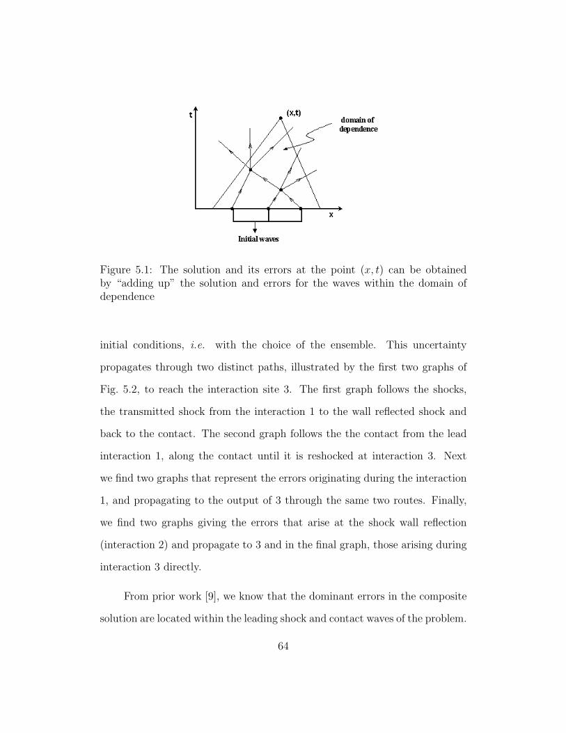
Figure 5.1: The solution and its errors at the point (x, t) can be obtainedby “adding up” the solution and errors for the waves within the domain ofdependence
initial conditions, i.e. with the choice of the ensemble. This uncertainty
propagates through two distinct paths, illustrated by the first two graphs of
Fig. 5.2, to reach the interaction site 3. The first graph follows the shocks,
the transmitted shock from the interaction 1 to the wall reflected shock and
back to the contact. The second graph follows the the contact from the lead
interaction 1, along the contact until it is reshocked at interaction 3. Next
we find two graphs that represent the errors originating during the interaction
1, and propagating to the output of 3 through the same two routes. Finally,
we find two graphs giving the errors that arise at the shock wall reflection
(interaction 2) and propagate to 3 and in the final graph, those arising during
interaction 3 directly.
From prior work [9], we know that the dominant errors in the composite
solution are located within the leading shock and contact waves of the problem.
64
A portion of these errors are simple resolution errors. This means that they
are errors due to the difference between the numerical and the exact wave
forms as traveling waves. This portion of the error is independent of the wave
interactions, and in the variables we use to describe the traveling waves, and
shows up in the wave width only. Any other errors, e.g. in strength or position,
or errors in width beyond these resolution errors can be attributed to the wave
interactions.
Now we explain in detail the definition of each of the terms associated
with these graphs. The simplest is the last. It is the error created during
the solution of the interaction at Riemann problem case 3. For this term,
we accept the numerical input to case 3 (as defined by a coarse grid solution,
including the numerical error). This input data is solved using both a fine grid
and a coarse grid, and the difference is the error associated with this graph.
The same formula applied to the initial point of the other graphs, defines the
beginning of each of the graphs 3 - 5. From this input error, we proceed as
follows: The error is transmitted without change along the edges of the graph.
For graph 3, the error is transmitted from output of the first interaction of
the graph, that is the pure transmitted shock wave output of interaction case
1 to the input of interaction case 2 in the same graph. The case 3 Riemann
problem then sees this error as an initial uncertainty and transforms it via a
linear transformation, to an output error or uncertainty located at the output
of interaction 3. The definition of the other graphs is similar, containing a
sequence of linear transformations, one for each Riemann problem the error
signal passes through.
65

Figure 5.2: Schematic graphs illustrating all contributions to the errors or un-certainty in the output from a single Riemann solution, namely the reshockinteraction (case 3) of the reflected shock from the wall as it crosses the con-tact. The numbers labeling the black circles refer to the Riemann interactionscontributing to the error. The letter I in the first two diagrams indicates inputuncertainty.
We develop these formulas explicitly for the first two graphs of Fig. 5.2,
representing one component of the propagation of the initial uncertainty (ini-
tial ensemble) to the output uncertainty of interaction 3. The initial uncer-
tainty is reflected in the wave strength variables, according to the definition
of the ensemble of initial conditions. The transmission of the mean values
through a linear model is standard and is not detailed here. The transforma-
tion of the variance follows formulas from Chap. 2. Let B(l) with matrix entries
β(l)jk be the matrix that gives the linear transformation of these variables due
to interaction l, as in (2.10). We note that the matrix entries β(l)jk are defined
by the ωi columns and ωo rows of Table 3.1 (linear; l = 1), Table 3.2 (l = 2),
66

and Table 3.3 (l = 3). The output to interaction 3 has three components, and
we compute the variance of each, labeled j = 1, 2, 3. By formula (2.13), we
have
Var ωo(3)j = (β
(3)j2 )2Var ω
i(3)2 = (β
(3)j2 )2Var ω
o(2)1
= (β(3)j2 )2(β
(2)11 )2Var ω
i(2)1 = (β
(3)j2 )2(β
(2)11 )2Var ω
o(1)3
= (β(3)j2 )2(β
(2)11 )2
2∑k=1
Var (β(1)3k )2ω
i(1)k (5.3)
This formula can be evaluated explicitly. We denote the LHS as SB1 in accor-
dance with (5.2).
SB1 =
⎛⎜⎜⎜⎜⎝
0.3122 0.6452
0.8092 0.1242
0.1422 0.4682
⎞⎟⎟⎟⎟⎠⎛⎝ 0
Var (wi32 )
⎞⎠
=
⎛⎜⎜⎜⎜⎝
0.3122 0.6452
0.8092 0.1242
0.1422 0.4682
⎞⎟⎟⎟⎟⎠ 0.7152
⎛⎝ 0 0
1.0012 0.3472
⎞⎠⎛⎝ Var (wi
1(t = 0))
Var (wi2(t = 0))
⎞⎠(5.4)
Similarly, the variance associated with the second graph can be evaluated
as
SB2 =
⎛⎜⎜⎜⎜⎝
0.3122 0.6452
0.8092 0.1242
0.1422 0.4682
⎞⎟⎟⎟⎟⎠⎛⎝ Var (wi3
1 )
0
⎞⎠
=
⎛⎜⎜⎜⎜⎝
0.3122 0.6452
0.8092 0.1242
0.1422 0.4682
⎞⎟⎟⎟⎟⎠⎛⎝ 0.0002 0.9112
0 0
⎞⎠⎛⎝ Var (wi
1(t = 0))
Var (wi2(t = 0))
⎞⎠ (5.5)
67
We also need to calculate formulas giving the transmission of position errors
through the various Riemann problems. For interaction with a wall (e.g. case
2), the formula is elementary. Assuming no error in the wall position, let pi and
po denote input and output position errors for a reflection off of a stationary
wall, where the output is due transmission of error, i.e. due only to the input,
as opposed to Chap. 3, where there is no input position error and the output
position error is created during the interaction. Then we have
po = pi vo
vi(5.6)
where vi and vo are the incoming and outgoing wave speeds for the waves
involved in the wall reflection. For the interaction of two incoming waves, the
result is slightly more complicated. Each of the two terms in the formulas
below is due to the input error in one of the input waves. That error can be
computed by (5.6) if we perform the analysis in the frame in which the other
wave is stationary. The result is
po1 =
pi1(v
o1 − vi
2) + pi2(v
i1 − vo
1)
vi1 − vi
2
(5.7)
po2 =
pi1(v
o2 − vi
2) + pi2(v
i1 − vo
2)
vi1 − vi
2
(5.8)
po3 =
pi1(v
o3 − vi
2) + pi2(v
i1 − vo
3)
vi1 − vi
2
(5.9)
where pij is the position error of the incoming contact wave (j = 1) or left facing
shock (j = 2). The complete position error model is obtained by adding the
68
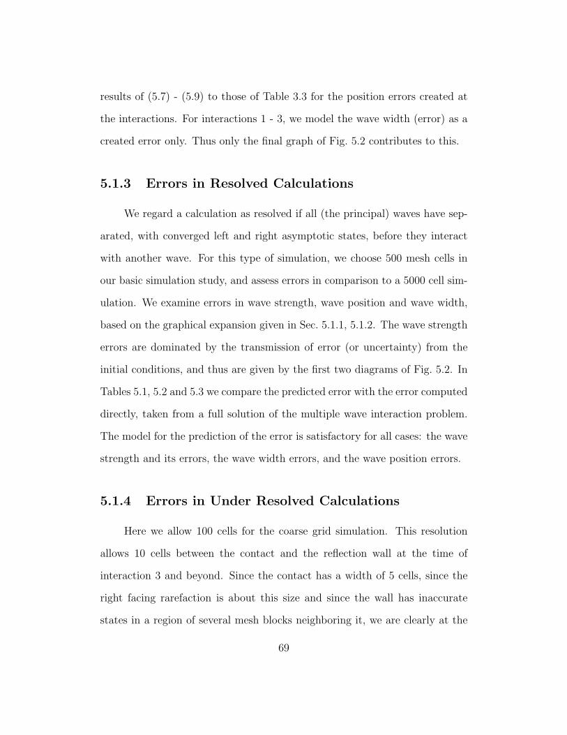
results of (5.7) - (5.9) to those of Table 3.3 for the position errors created at
the interactions. For interactions 1 - 3, we model the wave width (error) as a
created error only. Thus only the final graph of Fig. 5.2 contributes to this.
5.1.3 Errors in Resolved Calculations
We regard a calculation as resolved if all (the principal) waves have sep-
arated, with converged left and right asymptotic states, before they interact
with another wave. For this type of simulation, we choose 500 mesh cells in
our basic simulation study, and assess errors in comparison to a 5000 cell sim-
ulation. We examine errors in wave strength, wave position and wave width,
based on the graphical expansion given in Sec. 5.1.1, 5.1.2. The wave strength
errors are dominated by the transmission of error (or uncertainty) from the
initial conditions, and thus are given by the first two diagrams of Fig. 5.2. In
Tables 5.1, 5.2 and 5.3 we compare the predicted error with the error computed
directly, taken from a full solution of the multiple wave interaction problem.
The model for the prediction of the error is satisfactory for all cases: the wave
strength and its errors, the wave width errors, and the wave position errors.
5.1.4 Errors in Under Resolved Calculations
Here we allow 100 cells for the coarse grid simulation. This resolution
allows 10 cells between the contact and the reflection wall at the time of
interaction 3 and beyond. Since the contact has a width of 5 cells, since the
right facing rarefaction is about this size and since the wall has inaccurate
states in a region of several mesh blocks neighboring it, we are clearly at the
69
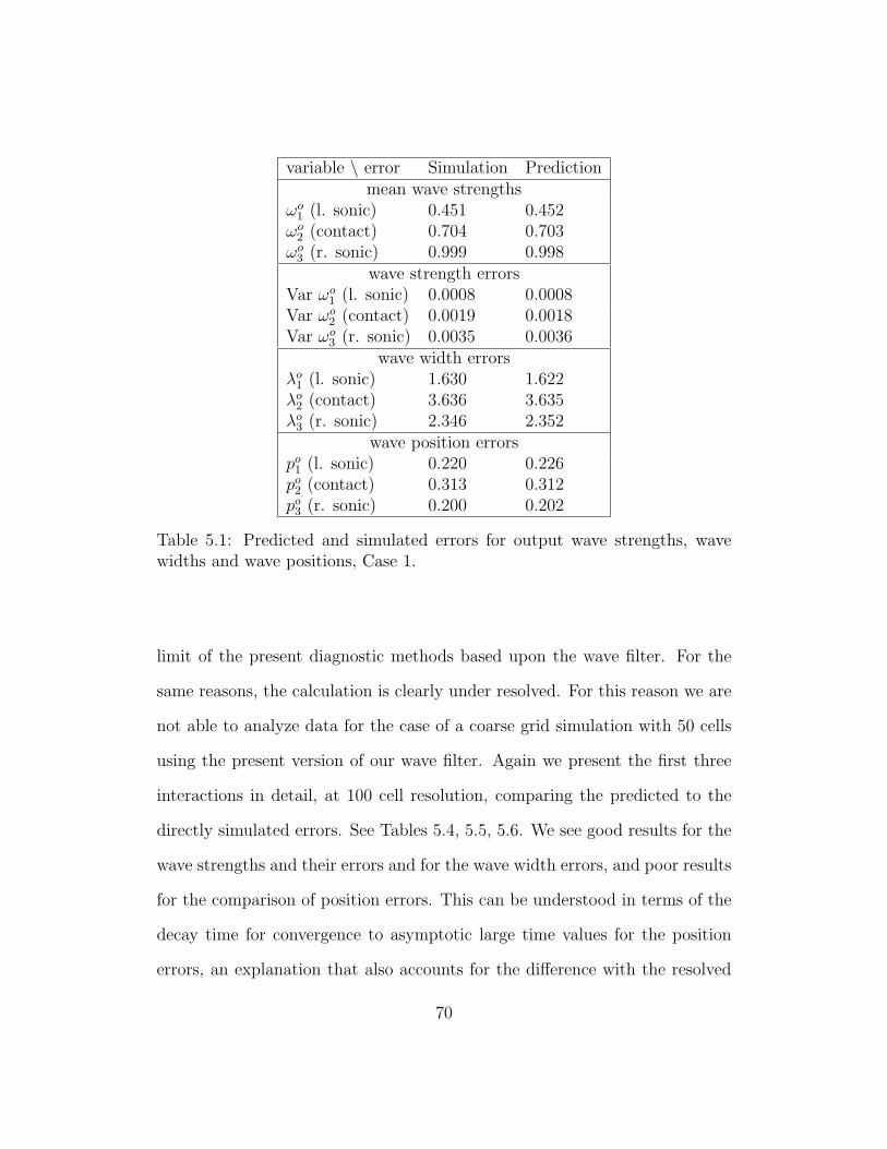
variable \ error Simulation Predictionmean wave strengths
ωo1 (l. sonic) 0.451 0.452
ωo2 (contact) 0.704 0.703
ωo3 (r. sonic) 0.999 0.998
wave strength errorsVar ωo
1 (l. sonic) 0.0008 0.0008Var ωo
2 (contact) 0.0019 0.0018Var ωo
3 (r. sonic) 0.0035 0.0036wave width errors
λo1 (l. sonic) 1.630 1.622
λo2 (contact) 3.636 3.635
λo3 (r. sonic) 2.346 2.352
wave position errorspo
1 (l. sonic) 0.220 0.226po
2 (contact) 0.313 0.312po
3 (r. sonic) 0.200 0.202
Table 5.1: Predicted and simulated errors for output wave strengths, wavewidths and wave positions, Case 1.
limit of the present diagnostic methods based upon the wave filter. For the
same reasons, the calculation is clearly under resolved. For this reason we are
not able to analyze data for the case of a coarse grid simulation with 50 cells
using the present version of our wave filter. Again we present the first three
interactions in detail, at 100 cell resolution, comparing the predicted to the
directly simulated errors. See Tables 5.4, 5.5, 5.6. We see good results for the
wave strengths and their errors and for the wave width errors, and poor results
for the comparison of position errors. This can be understood in terms of the
decay time for convergence to asymptotic large time values for the position
errors, an explanation that also accounts for the difference with the resolved
70

variable \ error Simulation Predictionmean wave strengths
ωo1 (l. sonic) 0.713 0.714
wave strength errorsVar ωo
1 (l. sonic) 0.0018 0.0018wave width errors
λo1 (l. sonic) 1.868 1.869
wave position errorspo
1 (l. sonic) -0.118 -0.092
Table 5.2: Predicted and simulated errors for output wave strengths, wavewidths and wave positions, Case 2.
case, for which the simulated and predicted position errors agree. The position
errors have a relatively slower decay time. The other three quantities show a
high level of agreement between the resolved and under resolved cases. The
wave width error is expressed in grid units, and so should be the same in the
two cases differing in grid resolution only. For the wave strength entries, the
lack of dependence on grid resolution is due to the fact that these quantities are
dominated by the uncertainty expressed in the ensemble of initial conditions,
which is independent of grid resolution.
5.2 Composite Shock Interaction Problems in Spherical
Flows
The main point of this section is to formulate and validate the multipath
scattering formula of Sec. 5.1 for analysis of spherical flow errors.
71

variable \ error Simulation Predictionmean wave strengths
ωo1 (l. sonic) 0.520 0.519
ωo2 (contact) 0.674 0.674
ωo3 (r. sonic) 0.306 0.305
wave strength errorsVar ωo
1 (l. sonic) 0.0009 0.0010Var ωo
2 (contact) 0.0012 0.0013Var ωo
3 (r. sonic) 0.0004 0.0004wave width errors
λo1 (l. sonic) 2.097 1.982
λo2 (contact) 5.027 4.918
λo3 (r. sonic) 2.875 3.033
wave position errorspo
1 (l. sonic) -0.097 -0.105po
2 (contact) -0.003 0.013po
3 (r. sonic) -0.151 -0.134
Table 5.3: Predicted and simulated errors for output wave strengths, wavewidths and wave positions, Case 3.
5.2.1 The Multipath Error Analysis Fromula
We consider the repeated interactions of a spherically symmetric shock
wave with a spherical contact located near the origin. The base case for each
wave interaction coincides with the base case assumed for the interactions
studied in Chap. 4. The transmitted shock, after interaction with the contact,
progresses to interact with (i.e. reflect off) the origin. This interaction was
also studied in Chap. 4. Subsequently, there are a number of reverberations,
of reflected rarefaction and compression waves, between the contact and the
origin. The interactions are illustrated by the space time contour plots of
the density, shown in Fig. 4.1 (left), and Fig. 4.1 (right) shows the type and
72

variable \ error Simulation Predictionmean wave strengths
ωo1 (l. sonic) 0.451 0.452
ωo2 (contact) 0.741 0.703
ωo3 (r. sonic) 0.996 0.998
wave strength errorsVar ωo
1 (l. sonic) 0.0008 0.0008Var ωo
2 (contact) 0.0022 0.0018Var ωo
3 (r. sonic) 0.0036 0.0036wave width errors
λo1 (l. sonic) 1.381 1.621
λo2 (contact) 3.498 3.635
λo3 (r. sonic) 2.347 2.352
wave position errorspo
1 (l. sonic) 0.972 0.226po
2 (contact) 1.539 0.312po
3 (r. sonic) 0.785 0.202
Table 5.4: Case 1. The contact-shock interaction (step up). Errors for outputwave strengths, wave widths and wave position. Comparison of under resolvedsimulation and prediction.
location of the waves determined by the wave filter analysis program.
We first appeal to the fine grid simulation data (as a stand in for the exact
solution) to develop or parameterize an affine linear model for the output
wave strengths at interaction j in terms of the input wave strengths. This
formula, considered variationally, also yields a model for the transmission of
error/uncertainty through interaction j. We additionally initialize comparable
input on the fine and coarse grids at interaction j, so that the difference
between the fine and coarse grid solutions is the created error at interaction j.
The created error, C(j)s , in the wave strength w at interaction j is thus defined
73

variable \ error Simulation Predictionmean wave strengths
ωo1 (l. sonic) 0.721 0.712
wave strength errorsVar ωo
1 (l. sonic) 0.0018 0.0018wave width errors
λo1 (l. sonic) 1.718 1.871
wave position errorspo
1 (l. sonic) -0.401 -0.092
Table 5.5: Case 2. The shock crossing equal shock (wave reflection) interaction.Errors for output wave strengths, wave width and wave position. Comparisonof under resolved simulation and prediction.
as
C(j)s = coarse − fine = w
o(j)s(c) − w
o(j)s(f) .
Here the three output waves are indexed form left to right by s, 1 ≤ s ≤ 3.
The superscripts o and i represent output and input strengths respectively,
and the subscripts f and c represent fine and coarse grid solutions.
The linear regression, or linear approximate formula for the output wave
strength at interaction j is obtained from the fine grid simulation data,
wo(j)s(f) = α(j)
s +2∑
k=1
β(j)sk w
i(j)k(f) . (5.10)
We use this formula variationally to obtain a formula for the transmission of
input error δwi(j)k . The input error itself is a combination of transmitted input
uncertainties Ic, Is and created errors C(i)s also transmitted from interactions
74

variable \ error Simulation Predictionmean wave strengths
ωo1 (l. sonic) 0.523 0.514
ωo2 (contact) 0.669 0.705
ωo3 (r. sonic) 0.318 0.315
wave strength errorsVar ωo
1 (l. sonic) 0.0009 0.0010Var ωo
2 (contact) 0.0013 0.0013Var ωo
3 (r. sonic) 0.0005 0.0004wave width errors
λo1 (l. sonic) 1.964 2.000
λo2 (contact) 4.606 4.928
λo3 (r. sonic) 2.169 3.029
wave position errorspo
1 (l. sonic) -0.551 -0.103po
2 (contact) 0.301 0.015po
3 (r. sonic) 0.432 -0.131
Table 5.6: Case 3. The contact-shock interaction (step down). Errors foroutput wave strengths, wave width and wave position. Comparison of underresolved simulation and prediction.
i < j,
δwo(j)s(f) =
2∑k=1
β(j)sk δw
i(j)k . (5.11)
A source S(i)r of errors contributes to the output error through wave interaction
diagrams g ∈ G(j)s(i)r , which connect the rth source at interaction i to the sth
output at the interaction j. Such diagrams were introduced in Sec. 5.1. A
shock wave as input to an intermediate interaction m with radius r(m) in a
diagram g ∈ G is propagated from the previous interaction m′ occurring at
the radius r(m′) according to a power law. The power law gives the definition
of a propagator with a proper power a(m,g) for the m′ m bond of the diagram
75
Figure 5.3: Schematic graphs, showing all six wave diagram contributionsto the errors or uncertainty in the output from a single Riemann solution,namely the reshock interaction (numbered 3 in the right frame of Fig. 4.1) ofthe reflected shock from the origin as it crosses the contact.
g,
P(m)(m′) =
(r(m)
r(m′)
)a(m,g)
. (5.12)
We define γ(m)sk for the sth output and the kth input at interaction m as the
multiple of a coefficient and a propagator, which are defined by a bond in the
diagram g (i.e.β is related to g and P to g)
γ(m)sk = β
(m)sk P(m)
(m′) . (5.13)
The coarse grid output error is the sum of the transmitted errors from (5.11)
and the error created at interaction j,
δwo(j)s(c) =
∑1≤r≤30≤i≤j
∑g∈G(j)s
(i)r
CgS(i)r , (5.14)
76
where Cg =∏
B(g)γ
(m)sk and the product runs over all bonds B(g) of the diagram
g. Observe that the created error at interaction j is included in the i = j term
in (5.14).
At the output to the interaction 3, we have the following closed form
expression for the mean,
〈δwo(3)s(c) 〉 = γ
(3)s1 γ
(2)11 〈C(1)
1 〉 + γ(3)s2 〈C(1)
2 〉 + γ(3)s1 〈C(2)
1 〉 + 〈C(3)s 〉 . (5.15)
Observe that 〈Is〉 = 〈Ic〉 = 0, so that with a linear propagation model and
assumed mean zero initial uncertainty, the two initial uncertainties do not con-
tribute to the mean error. We assume statistical independence of the sources,
to obtain a closed form expression for the variance of the error,
Var δwo(3)s(c) =
{(γ
(3)s1 γ
(2)11 γ
(1)11
)2
+(γ
(3)s2 γ
(1)21
)2}
Var Ic
+
{(γ
(3)s1 γ
(2)11 γ
(1)12
)2
+(γ
(3)s2 γ
(1)22
)2}
Var Is
+(γ
(3)s1 γ
(2)11
)2
Var C(1)1 +
(γ
(3)s2
)2
Var C(1)2
+(γ
(3)s1
)2
Var C(2)1 + Var C(3)
s . (5.16)
5.2.2 Results
We analyze errors at the output to interaction 3 directly, comparing the
100 mesh and 500 mesh simulation to a 2000 mesh, fine grid simulation, here
taken as a substitute for the exact solution. These errors are compared to those
generated by adding up and propagating errors from the input data and from
77

variable \ error Simulation Prediction Simulation Prediction100 vs. 2000 mesh 500 vs. 2000 meshwave strength errors and propagated initial uncertainties
δo1 (l. sonic) 0.04±2(0.03) 0.03±2(0.02) 0.01±2(0.02) 0.009±2(0.01)
δo2 (contact) 0.14±2(0.05) 0.12±2(0.02) 0.03±2(0.01) 0.03±2(0.008)
δo3 (r. sonic) -0.02±2(0.02) -0.02±2(0.01) -0.006±2(0.005) -0.007±2(0.004)
mean wave width errors mean wave width errorsλo
1 (l. sonic) 3.04 2.83 2.63 2.72λo
2 (contact) 5.36 6.11 5.56 6.08λo
3 (r. sonic) 2.71 3.04 2.92 2.98mean wave position errors mean wave position errors
po1 (l. sonic) 1.25 0.23 0.12 0.18
po2 (contact) 0.43 0.06 0.05 0.04
po3 (r. sonic) -0.73 -0.15 -0.08 -0.11
Table 5.7: Predicted and simulated errors for output wave strengths, wavewidths and wave positions, output to interaction 3. The inward rarefactionand contact strengths are expressed dimensionlessly as Atwood numbers. Theoutward shock strengths are in the units of Mach number. The width andposition errors are in mesh units. The wave strength errors are expressed asmean ± 2σ where σ is the ensemble STD of the error/uncertainty.
each of the interactions 1 to 3, using the multipath scattering formula. Thus,
for example, a position error as input to interaction 1 is translated geometri-
cally to a position error for the output to interaction 1 via simple geometric
considerations as in Sec.5.1. This error is propagated to an input error for
interaction 2 through solutions of radial differential equations. Propagation
continues, and yields an error at the output to interaction 3. See Table 5.7.
The wave strength rows present the result of initial uncertainty propagated to
the output of interaction 3 as well as the accumulation of solution errors. The
multipath scattering formula gives reasonable prediction of error magnitudes
in all cases except the wave position errors for the under resolved (100 mesh)
78

simulation. We see that the created numerical solution errors are important.
We also find that a major portion of the created numerical solution errors
come from the second interaction, the shock reflection interaction.
In Figs. 5.4, 5.5, we present three pie charts representing fractional con-
tribution from each of the six interactions to the error variance for the inward
rarefaction, contact and outward shock, respectively, as output to interaction
3. From these charts, we can infer the relative importance between the in-
put uncertainty and the solution error and determine the contribution of each
interaction to the total error variance.
We also show the contributions of each interaction to the mean value of
the final total error. See Table. 5.8. We only show the values correspond-
ing to diagrams 3 to 6, as the contribution of the first two diagrams (input
uncertainties) is observed to be zero.
Wave Diagram I.R. C. O.S.Number 100 500 100 500 100 500
3 0.10 -0.01 -0.01 0.001 0.09 -0.0094 0.05 0.009 0.1 0.02 -0.02 -0.0045 -0.05 -0.005 0.006 0.0006 -0.04 -0.0046 -0.07 0.015 0.03 0.01 -0.05 0.01
Total Prediction 0.03 0.009 0.12 0.03 -0.02 -0.007Total Simulation 0.04 0.01 0.14 0.03 -0.02 -0.006
Table 5.8: The contribution of each interaction to the mean value of the totalerror in each of three output waves at the output to interaction 3, for 100 and500 mesh units. Units are dimensionless and represent the error expressed asa fraction of the total wave strength. The last two rows compare the totalof the mean error as given by the model to the directly observed mean error.The columns I.R., C., and O. S. are labeled as in Fig. 4.1, Right frame.
79

(a) Inward Rarefaction
(b) Contact
(c) Outward Shock
Figure 5.4: Pie charts showing the contribution of each wave interaction dia-gram to the error variance of the wave strength at the output of interaction 3,for a solution using 500 mesh units.
80

(a) Inward Rarefaction
(b) Contact
(c) Outward Shock
Figure 5.5: Pie charts showing the contribution of each wave interaction dia-gram to the error variance of the wave strength at the output of interaction 3,for a solution using 100 mesh units.
81

Chapter 6
Conclusion And Future Work in 2D Chaotic
Flows
6.1 Conclusion from 1D Flow Study
We have several main conclusions from the error study of numerical so-
lutions of 1D flow.
• From Chap. 2, 3 and 4, we showed that a very simple model of solution
error is sufficient for the study of (at least the present instance of) a
highly nonlinear problem. The error is linear in the input wave strengths.
• In Chap. 5, a composition law for combining errors and predicting er-
rors for composite interactions on the basis of an error model of the
simple constituent interactions has been formulated and validated. For
spherically symmetric shock physics problems, the main new difficulties
encountered were the non-constancy of the solution between interaction
events and the non-constancy of waves and errors between interactions.
82
For a planar geometry, the errors are constant between interactions, while
for a spherical geometry, the errors grow (if the wave which carries them
is moving inward) by a power law in the radius. Similarly outward mov-
ing waves and their errors weaken by a power law.
• In 1D flows of planar geometry, we find that although our formalism
allows for statistical errors in the ensemble that in fact, the dominant
part of all errors (excluding position errors) studied were deterministic,
in the sense that the ensemble mean error dominated the ensemble stan-
dard deviation. For spherical geometry, the composition model applied
to construct the variance of the error in the wave strength, generally
understates the STD by a factor generally between 1.5 and 2, for causes
not presently identified. Using the model, the total error is a sum of six
terms, each corresponding to a pattern of wave interactions and trans-
missions. Of these diagrams, two correspond to initial error, following
different transmission patterns, and four correspond to errors created
within the solution and transmitted to the output of the reshock inter-
action, where the errors are analyzed. We see that for a 500 cell grid,
the dominant error comes from the initial uncertainty, while for the 100
grid over 75% of the error arises within the numerical simulation. We
could conclude that for coarse grid simulations, there exists increased
importance of created errors.
• For planar case, the wave strength uncertainty which is dominated by
input uncertainty (i.e. the definition of the ensemble), is virtually un-
83
changed between the highly resolved and the under resolved simulations.
While for spherical case, this is not true. We concluded that for under
resolved spherical simulations, there exists increased importance of cre-
ated errors. The wave width errors are both expressed in grid units, and
are comparable between the two levels of resolution. The wave width
errors evidentially have a rapid relaxation to their asymptotic value.
• The primary solution errors created by the simulations are the wave
position errors in the under resolved simulations, on the order of a mesh
spacing. These errors are a transient phenomena, but become frozen
into the calculation as new interactions occur before the transient errors
have diminished. The wave position errors have a slow relaxation to
asymptotic values.
• We find that the wave filter performs well as a diagnostic tool, but that its
limitation (in its present version) lies in assuming well separated waves.
Thus we are limited in the degree of under resolution that we can analyze,
in that all waves must be at least partially separated from one another
before entering into a new interaction.
To the extent that a more detailed modeling of these errors is important,
a more accurate model that includes transient effects will be important. Even
with these limitations, the methods and results appear to be promising, and
should be extended to less idealized problems.
These conclusions are established only under several simplifying assump-
tions, namely restriction to one spatial dimension, use of a simplified (gamma
84
law gas) equation of state, and consideration of only one numerical method.
Further studies are needed to determine the extent that these conclusions have
a general validity.
6.2 Future Work in 2D Chaotic Flows
We are to apply the statistical approach to error analysis for the prob-
lems considered here, namely chaotic CFD. By definition, chaotic flows are
ones which exhibit sensitive dependence on initial conditions. Generally, they
also exhibit sensitive dependence on other parameters, not only the physical
parameters which define the flow, but also the numerical parameters which
define the solution algorithm.
There is no shortage of important chaotic flow problems. We mention
climatology [1], turbulence [4, 29], fluid mixing [34], flow in porous media [27],
and turbulent combustion [30]. Here we consider a representative but rela-
tively simple chaotic flow, the Richtmyer-Meshkov instability resulting from
a shock passing through a density discontinuity. We consider this problem in
a perturbed circular (2D) geometry. Namely, a circular shock wave implodes
a perturbed circular interface, and the two circles may or may not be offset
relative to one another. The shock proceeds to the origin, where it is reflected,
and the reflected shock reshocks the now highly perturbed interface, giving
rise to a highly chaotic flow. See Fig. 6.1.
85
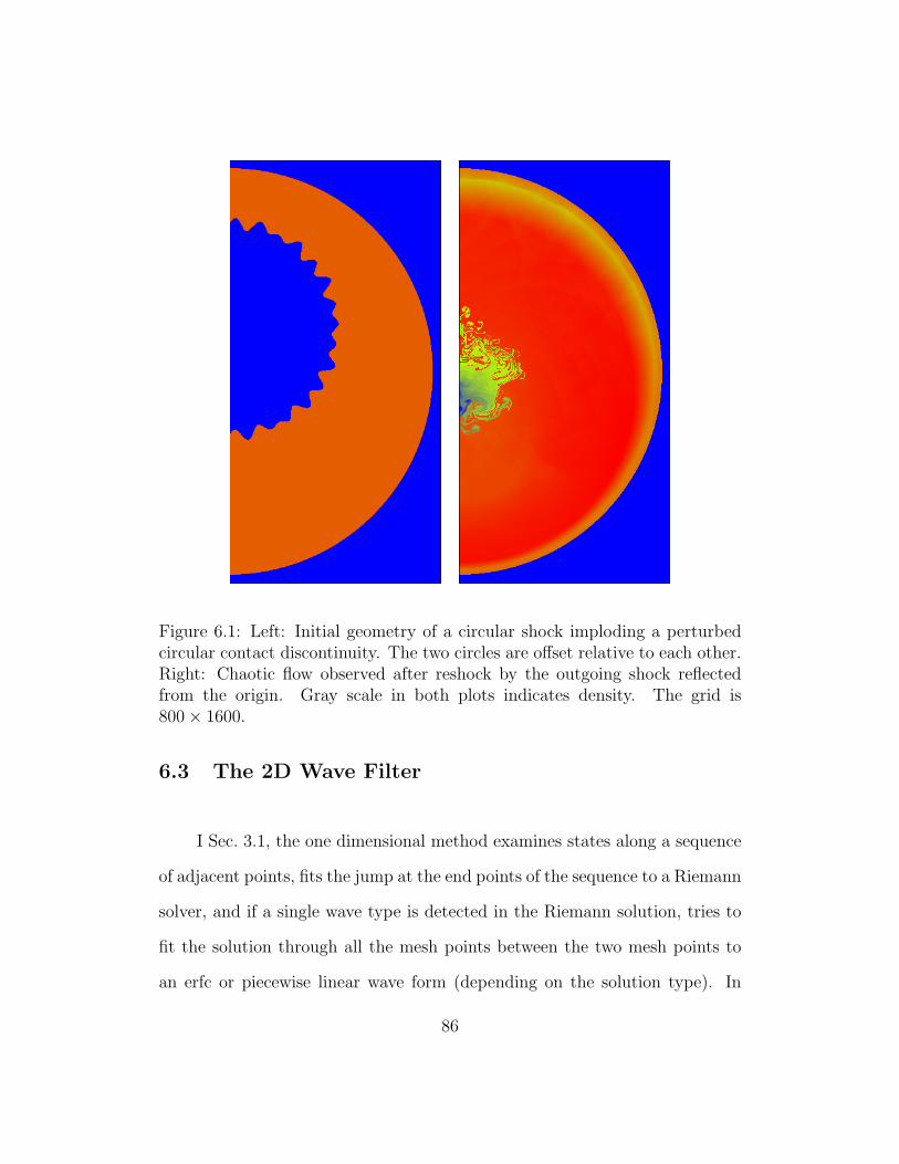
Figure 6.1: Left: Initial geometry of a circular shock imploding a perturbedcircular contact discontinuity. The two circles are offset relative to each other.Right: Chaotic flow observed after reshock by the outgoing shock reflectedfrom the origin. Gray scale in both plots indicates density. The grid is800 × 1600.
6.3 The 2D Wave Filter
I Sec. 3.1, the one dimensional method examines states along a sequence
of adjacent points, fits the jump at the end points of the sequence to a Riemann
solver, and if a single wave type is detected in the Riemann solution, tries to
fit the solution through all the mesh points between the two mesh points to
an erfc or piecewise linear wave form (depending on the solution type). In
86

[11], this algorithm was extended to two dimensional flows. Starting from
an arbitrary point and in an arbitrary direction, a 1D wave filter looks for a
significant indication of a single wave type. The central location and direction
in which this single wave type occurs most clearly is the predictor for the wave
front position and normal. The predictor for the tangent to the wave front is
the normal to the predictor normal, passing through the predictor position.
Finding points at unit mesh spacing along this predictor for the tangent, we
repeat the 1D construction to find the best fitting position for the wave front.
From this construction, we have three points on the wave front, one to the left,
one to the right and one at the original location where the wave was detected.
We fit a circle to these three points, giving a corrected wave front position and
normal. For the present problem, with its approximate circular symmetry, and
our average of state variables over a 45o angular sector, we average the shock
position data in these sectors also to yield sector-averaged shock positions.
This algorithm is here applied in 2D for the first time, and we find some
modifications are needed for efficiency. First, as we are only interested in
the detection of shock waves, all the 1D passes only look for shock waves.
Secondly, we can prune the initial search locations and directions, omitting
points and directions in which an initial analysis indicates no activity. The
wave front data analysis is performed at a fixed time interval equal to six time
steps on the coarse grid, and occupies less than 10% of the total solution time.
A new wave type, the edge (inner or outer) of the mixing zone is also needed,
and for this purpose a new wave filter is constructed. We follow previously
accepted ideas in the analysis of Rayleigh-Taylor mixing data, and look for
87
the 5% and 95% volume fraction contours. For the present problem, with
approximate circular symmetry, we look for the 5% and 95% volume fraction
contours within a 45o sector. The location of these 5% and 95% contours can
be a noisy diagnostic for the edge of the mixing zone, which occasionally moves
abruptly as a function of time. While we have not solved this problem, we
have avoided it for the data presented in this paper.
In Fig. 6.2, we plot the space time contours in r, t space for the inward and
reflected shocks and for the inner and outer edges of the mixing zone. We have
adjusted the tolerances in the automated filter so that it picks up exclusively
the strong waves we are trying to locate (and thus misses numerous weak
waves). The thresholds are set in the variable (P2 − P1)× (pressure ratio +
Atwood number). The shock wave filter does not depend on angular averaging.
The angular dependence of the shock wave for a sequence of times is shown
in Fig. 6.3. This figure illustrates the robustness of the wave filter tool in its
2D application. The ripples in the wave front in the left frame near the center
(vertically) of the figure are at the time of passage of the shock front through
the perturbed interface, and reflect defraction events at the shock front to
advance or retard local portions of the shock front. Similar ripples occur in
the outgoing shock angular dependence during its transit through the mixing
zone. See Fig. 6.3, right frame, near the bottom.
6.4 Problem Formulation
We consider a computational domain x, y ∈ [0, 25] × [−25, 25] (units of
mm). With r denoting the radial coordinate in the x, y plane, the initial
88
contact is perturbed from a circle at r = 12.5. Outside this contact is a stiff-
ened gamma law gas, representing tin, with parameters given approximately
by γ = 3.72, p∞ = 0.15, e∞ = 0.0. Inside the contact is also a stiffened
gamma law gas, representing lucite, with approximate parameters γ = 1.85,
p∞ = 0.03, e∞ = 0.0. A constant pressure boundary is located at r = 24. The
initial ambient pressure is p = 10−6, and the imposed pressure at the boundary
is p = 0.687, giving rise to an inward propagating Mach M = 2 shock at t = 0.
The densities are approximately ρtin = 7.3 and ρlucite = 1.2 at t = 0, giving
an Atwood number A = (ρ2 − ρ1)/(ρ2 + ρ1) = 0.72. We consider a series of
grids, with sizes 100 × 200, 200 × 400, 400 × 800, and 800 × 1600. Errors will
be assessed in comparison of adjacent grid sizes. The runs continue until after
the passage of the reflected shock through the contact interface (reshock), and
terminate before the rarefaction wave which results from the reflected shock
interaction with the constant pressure boundary contaminates (very much of)
the rest of the flow. For the present problem dimensions, this time is t = 80.
With this convention, we observe errors at three levels of mesh refinement in
this study.
The contact interface has been perturbed by sine waves to have the initial
configuration
r(θ) = r0
(1 +
∑n
an sin(nθ)
), (6.1)
θ ∈ [−π/2, π/2]. Here r0 = 12.5 and sine modes are selected so that the
imposed reflection symmetry at θ = ±π/2 leads to a smooth curve. The
sum over n ranges from nmin = 8 to nmax = 16, so that the average number
of observed modes in the initial perturbation is about 12. The coefficients
89

an are chosen as Gaussian random variables, with mean zero and STD 0.2,
based on the C random number generator erand48(), mapped into a Gaussian
distribution. The observed mean peak to peak amplitude, determined by this
STD, is 0.25. Successive calls to the random number generator generate the
ensemble of initial conditions used in this study.
For the non-offset simulations, the circles defining the pressure boundary
conditions (and the initial shock) and the contact are both centered at the ori-
gin. For the offset simulations, the circle defining the (pre-perturbed) contact
has a center at x = 0, y = 5.
90
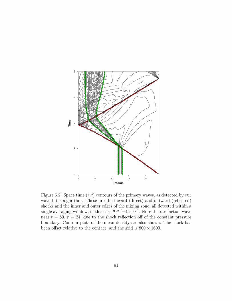
Radius
Tim
e
0 5 10 15 20
020
4060
80
Figure 6.2: Space time (r, t) contours of the primary waves, as detected by ourwave filter algorithm. These are the inward (direct) and outward (reflected)shocks and the inner and outer edges of the mixing zone, all detected within asingle averaging window, in this case θ ∈ [−45o, 0o]. Note the rarefaction wavenear t = 80, r = 24, due to the shock reflection off of the constant pressureboundary. Contour plots of the mean density are also shown. The shock hasbeen offset relative to the contact, and the grid is 800 × 1600.
91

Angle
Rad
ius
-90 -60 -30 0 30 60 900
5
10
15
20
25
Angle
Rad
ius
-90 -60 -30 0 30 60 900
5
10
15
20
25
Figure 6.3: Radial shock position as a function of angle for a series of times.The grid level is 200 and there is no offset of the center. Left: inward shock,right: outward shock.
92

Chapter 7
Appendix
7.1 Appendix 1: The Rest of Statistical Numerical Rie-
mann Problems in Planar Flows
For each of the 10 Riemann problems of Fig. 2.4, Right, we vary the
wave strength and for contacts only, we vary the wave width. Three variables
defining one reference state are not varied in this study; presumably similar
conclusions would be reached if they were also varied. We have two goals
in selecting the reference variables to hold fixed. If one of the states has a
reference ambient velocity, for example a velocity v = 0 for a state near a wall,
we want to preserve this property and freeze this velocity. For the pressure
and density values, we generally freeze those on the smaller side of the waves,
as this gives a more meaningful variation of the state, uniformly specified as
10% of the wave strength, as defined in Chap. 2.
93

7.1.1 Rarefaction Crossing Rarefaction Interaction (Case
4)
Here we study the reflection of the rarefaction off the wall, a special case
of the rarefaction crossing rarefaction interaction. We have one input and one
output wave width parameter, both for the rarefaction. The Rimann problem
was set up as Fig. 7.1. And we assume that at interaction location the input
rarefaction and the output rarefaction have the same width. The rarefaction
width has the form constant + initial width + rate × time. The entry λo1 in
Table 7.1 refers to the constant, which gives an offset for the centering of the
rarefaction wave. We find very small errors in the rate, not tabulated here.
This entry is expressed in mesh units. We form a linear model for this constant
in Table 7.1.
Figure 7.1: Problem 4: Rarefaction-wall. The right state velocity v = 0.0is fixed and the left state densities and pressures are held fixed. The inputrarefaction wave width is an input parameter. Same comments applied to latercases.
94

variable \ coef const ωi1 error
(r. sonic) L∞ STDωo
1 (l. sonic) 0.146 0.657 0.181% 0.0003λo
1 (l. sonic) 3.832 2.091 5.056% 0.096po
1 (l. sonic) 0.071 -0.237 8785% 0.006
Table 7.1: Case 4. The SNRP defined by the crossing of two rarefactions.Expansion coefficients for output wave strengths (linear model) for input vari-ation ±10%.
Figure 7.2: Problem 5: Contact-rarefaction. The right state velocity v = 0.0is fixed and the left state densities and pressures are held fixed.
7.1.2 The Contact Rarefaction Interaction (Case 5)
After reflection from the wall, the transmitted rarefaction wave re-crosses
the deflected contact. We have two input wave width parameters, see Fig. 7.2,
one each for the contact and the rarefaction, and three output wave width
parameters, one each for the left rarefaction, the contact and the right com-
pression wave. According to the analysis of single isolated waves, the output
contact width is bounded after some 100 time steps. The Table 7.2 entry λo2
refers to this bounded width. We assume that at interaction the input rarefac-
tion and the output rarefaction have the same width. The rarefaction width
95
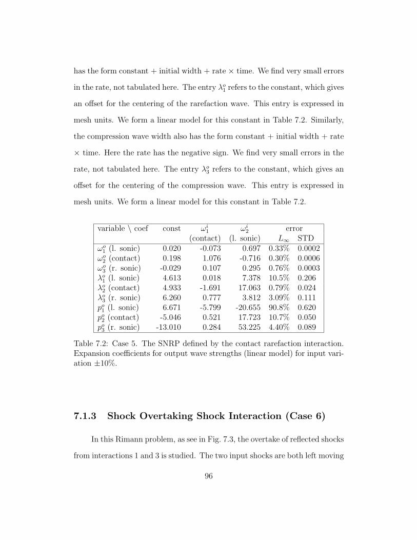
has the form constant + initial width + rate × time. We find very small errors
in the rate, not tabulated here. The entry λo1 refers to the constant, which gives
an offset for the centering of the rarefaction wave. This entry is expressed in
mesh units. We form a linear model for this constant in Table 7.2. Similarly,
the compression wave width also has the form constant + initial width + rate
× time. Here the rate has the negative sign. We find very small errors in the
rate, not tabulated here. The entry λo3 refers to the constant, which gives an
offset for the centering of the compression wave. This entry is expressed in
mesh units. We form a linear model for this constant in Table 7.2.
variable \ coef const ωi1 ωi
2 error(contact) (l. sonic) L∞ STD
ωo1 (l. sonic) 0.020 -0.073 0.697 0.33% 0.0002
ωo2 (contact) 0.198 1.076 -0.716 0.30% 0.0006
ωo3 (r. sonic) -0.029 0.107 0.295 0.76% 0.0003
λo1 (l. sonic) 4.613 0.018 7.378 10.5% 0.206
λo2 (contact) 4.933 -1.691 17.063 0.79% 0.024
λo3 (r. sonic) 6.260 0.777 3.812 3.09% 0.111
po1 (l. sonic) 6.671 -5.799 -20.655 90.8% 0.620
po2 (contact) -5.046 0.521 17.723 10.7% 0.050
po3 (r. sonic) -13.010 0.284 53.225 4.40% 0.089
Table 7.2: Case 5. The SNRP defined by the contact rarefaction interaction.Expansion coefficients for output wave strengths (linear model) for input vari-ation ±10%.
7.1.3 Shock Overtaking Shock Interaction (Case 6)
In this Rimann problem, as see in Fig. 7.3, the overtake of reflected shocks
from interactions 1 and 3 is studied. The two input shocks are both left moving
96

forward shocks, which are produced by interactions 1 and 3, respectively. And
theoretically, one left moving forward shock, one contact and one right moving
backward shock are produced. We ignore the output backward shock because
it is too weak(ωo3 = 0.017) to be recognized by the filter program. Therefore,
the position error po3 and the width error λo
3 are not presented here.
Figure 7.3: Problem 6: Shock-shock overtake (two waves of the same family).The left state is held fixed and the two wave strengths are varied.
However, with an improved post-processing program, we can still get all
input and output gas states, so all input and output strengths are studied
here.
This case is a step down problem. From the analysis of the Sec. 3.2,
the contact width will be modeled as ωc cc ∼ t1/3, where the coefficient cc is
affected to Mach number, and the t denotes the time steps counted from the
interaction time. This also is showed by the Fig. 7.4, in which we take a log
for the time step axis to show the linear relationship. The time steps starts
from 51, because the contact widths near interaction time are unstable, which
are deleted for better result. And the we observe an increase in width from 4
cells to 9 over 1000 time steps.
97

In this plot there is a noticeable small disturbance after 1000 time steps,
beyond an otherwise good linear relation. That disturbance is due to an
additional wave interaction with the contact at that time, therefore affects
the contact width after 1000 time steps. This interaction is not presented here
since it is not one of the major interactions, but still it can be seen in Fig. 2.4.
Figure 7.4: Because the width is entirely grid related, we record width in unitsof ∆x and time in units of the number of time steps.
Thus, in the Table 7.3 we interpret λo2t
1/3 or λo2 as the output contact wave
width, also in grid units, depending on the Mach number. For λo1, it is the
shock wave width and independent of time steps. And pak and ωa
k (k = 1, 2, 3
and a = i, o) represent position errors and wave strengths as usual.
The width of the left most input forward shock, which is from interaction
1, is 1 grid unit. And The width of the other input forward shock, which is
from interaction 3, is 2 grid units.
98
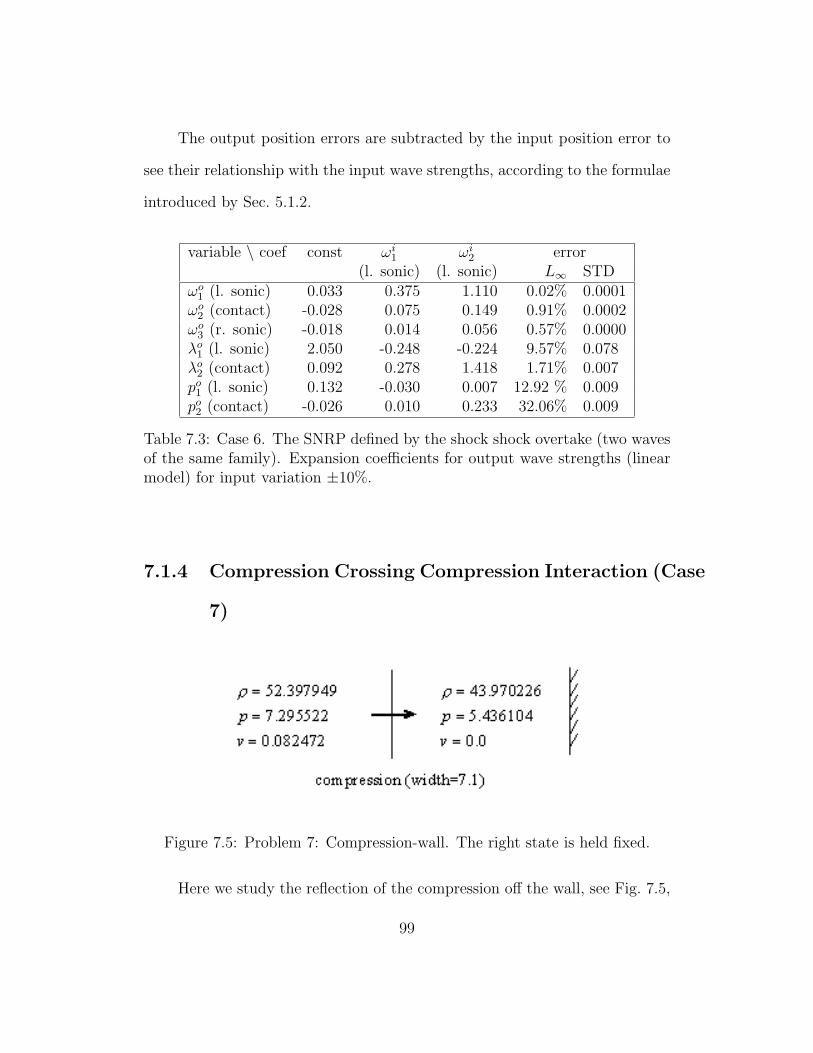
The output position errors are subtracted by the input position error to
see their relationship with the input wave strengths, according to the formulae
introduced by Sec. 5.1.2.
variable \ coef const ωi1 ωi
2 error(l. sonic) (l. sonic) L∞ STD
ωo1 (l. sonic) 0.033 0.375 1.110 0.02% 0.0001
ωo2 (contact) -0.028 0.075 0.149 0.91% 0.0002
ωo3 (r. sonic) -0.018 0.014 0.056 0.57% 0.0000
λo1 (l. sonic) 2.050 -0.248 -0.224 9.57% 0.078
λo2 (contact) 0.092 0.278 1.418 1.71% 0.007
po1 (l. sonic) 0.132 -0.030 0.007 12.92 % 0.009
po2 (contact) -0.026 0.010 0.233 32.06% 0.009
Table 7.3: Case 6. The SNRP defined by the shock shock overtake (two wavesof the same family). Expansion coefficients for output wave strengths (linearmodel) for input variation ±10%.
7.1.4 Compression Crossing Compression Interaction (Case
7)
Figure 7.5: Problem 7: Compression-wall. The right state is held fixed.
Here we study the reflection of the compression off the wall, see Fig. 7.5,
99
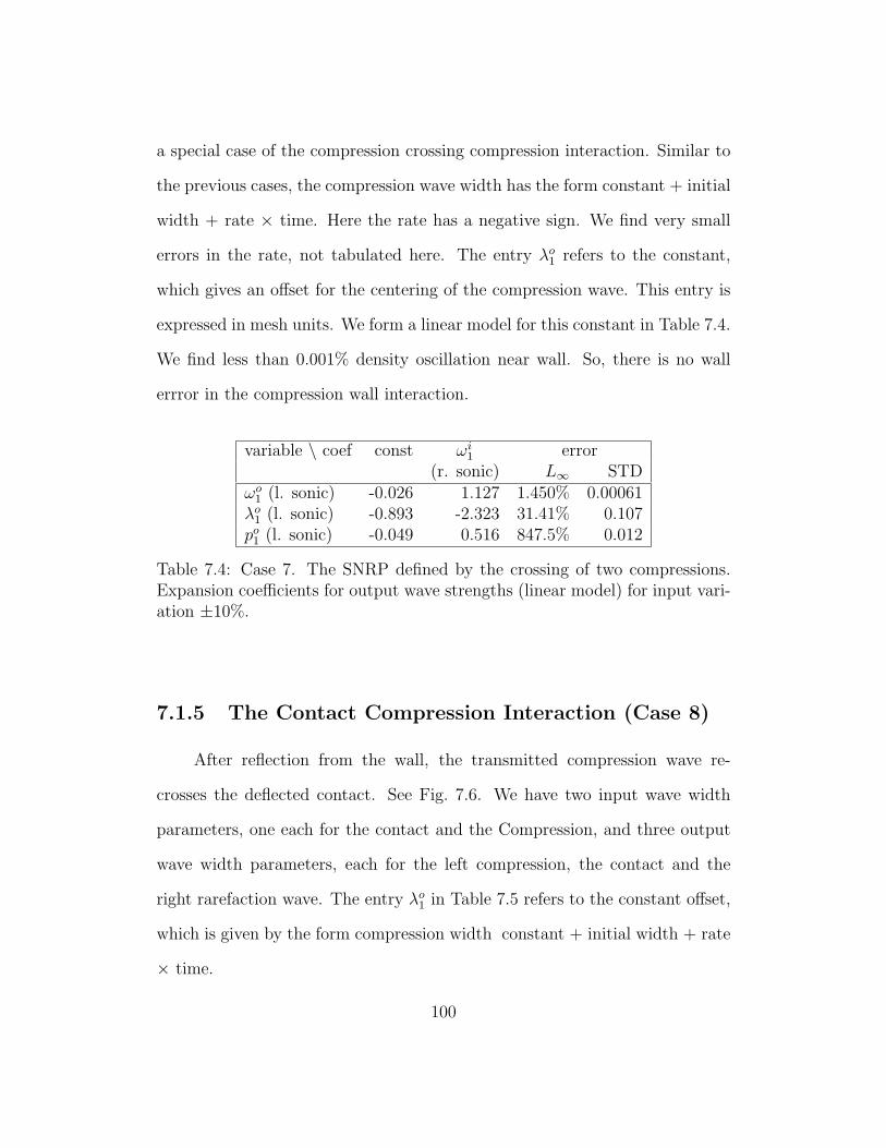
a special case of the compression crossing compression interaction. Similar to
the previous cases, the compression wave width has the form constant + initial
width + rate × time. Here the rate has a negative sign. We find very small
errors in the rate, not tabulated here. The entry λo1 refers to the constant,
which gives an offset for the centering of the compression wave. This entry is
expressed in mesh units. We form a linear model for this constant in Table 7.4.
We find less than 0.001% density oscillation near wall. So, there is no wall
errror in the compression wall interaction.
variable \ coef const ωi1 error
(r. sonic) L∞ STDωo
1 (l. sonic) -0.026 1.127 1.450% 0.00061λo
1 (l. sonic) -0.893 -2.323 31.41% 0.107po
1 (l. sonic) -0.049 0.516 847.5% 0.012
Table 7.4: Case 7. The SNRP defined by the crossing of two compressions.Expansion coefficients for output wave strengths (linear model) for input vari-ation ±10%.
7.1.5 The Contact Compression Interaction (Case 8)
After reflection from the wall, the transmitted compression wave re-
crosses the deflected contact. See Fig. 7.6. We have two input wave width
parameters, one each for the contact and the Compression, and three output
wave width parameters, each for the left compression, the contact and the
right rarefaction wave. The entry λo1 in Table 7.5 refers to the constant offset,
which is given by the form compression width constant + initial width + rate
× time.
100

Figure 7.6: Problem 8: Contact-compression. The right state velocity v = 0.0is fixed and the left state densities and pressures are held fixed.
7.1.6 Rarefaction Crossing Rarefaction Interaction (Case
9)
Figure 7.7: Problem 9: Rarefaction-wall. The right state velocity v = 0.0 isfixed and the left state densities and pressures are held fixed.
Case 9, as show in Fig. 7.7, is the reflection of the rarefaction off the wall
again. We used the same error model as in case 4.
7.1.7 The Contact Rarefaction Interaction (Case 10)
The Riemann Problem of case 10 is set up as Fig. 7.8. The output wave
strengths in case 10 are very weak (ωo1 = 0.033, ωo
2 = 0.674, ωo3 = 0.021). The
101

variable \ coef const ωi1 ωi
2 error(contact) (l. sonic) L∞ STD
ωo1 (l. sonic) 0.030 -0.039 0.601 3.46% 0.0008
ωo2 (contact) -0.043 0.973 0.442 0.71% 0.0011
ωo3 (r. sonic) -0.026 0.034 0.402 4.29% 0.0007
λo1 (l. sonic) 3.298 0.116 -1.510 13.2% 0.080
λo2 (contact) -0.240 -0.081 -4.584 3480% 0.432
λo3 (r. sonic) 3.758 -1.265 9.379 19.7% 0.273
po1 (l. sonic) -0.086 1.295 -1.609 95.0% 0.186
po2 (contact) 0.218 -0.273 0.068 195.3% 0.147
po3 (r. sonic) -0.519 -0.772 2.298 44.8% 0.153
Table 7.5: Case 8. The SNRP defined by the contact compression interaction.Expansion coefficients for output wave strengths (linear model) for input va-ration ±10%.
wave filter lacks sufficient precision to allow analysis of the errors in this case,
because their small size are not important in any case.
variable \ coef const ωi1 error
(r. sonic) L∞ STDωo
1 (l. sonic) 0.004 0.938 0.55% 0.0001λo
1 (l. sonic) -0.060 5.290 206% 0.067po
1 (l. sonic) 0.119 -1.948 1938% 0.013
Table 7.6: Case 9. The SNRP defined by the crossing of two rarefactions.Expansion coefficients for output wave strengths (linear model) for input vari-ation ±10%.
102
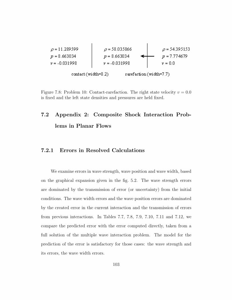
Figure 7.8: Problem 10: Contact-rarefaction. The right state velocity v = 0.0is fixed and the left state densities and pressures are held fixed.
7.2 Appendix 2: Composite Shock Interaction Prob-
lems in Planar Flows
7.2.1 Errors in Resolved Calculations
We examine errors in wave strength, wave position and wave width, based
on the graphical expansion given in the fig. 5.2. The wave strength errors
are dominated by the transmission of error (or uncertainty) from the initial
conditions. The wave width errors and the wave position errors are dominated
by the created error in the current interaction and the transmission of errors
from previous interactions. In Tables 7.7, 7.8, 7.9, 7.10, 7.11 and 7.12, we
compare the predicted error with the error computed directly, taken from a
full solution of the multiple wave interaction problem. The model for the
prediction of the error is satisfactory for those cases: the wave strength and
its errors, the wave width errors.
103
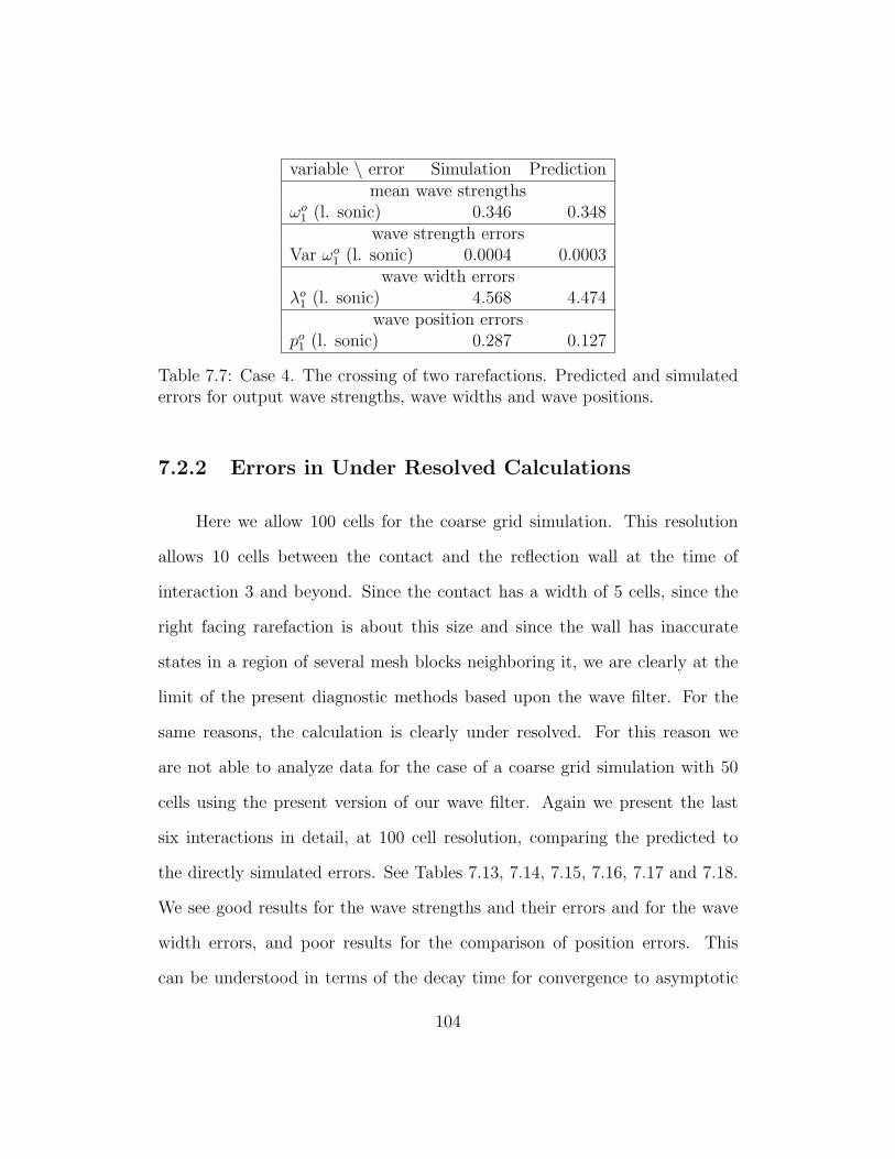
variable \ error Simulation Predictionmean wave strengths
ωo1 (l. sonic) 0.346 0.348
wave strength errorsVar ωo
1 (l. sonic) 0.0004 0.0003wave width errors
λo1 (l. sonic) 4.568 4.474
wave position errorspo
1 (l. sonic) 0.287 0.127
Table 7.7: Case 4. The crossing of two rarefactions. Predicted and simulatederrors for output wave strengths, wave widths and wave positions.
7.2.2 Errors in Under Resolved Calculations
Here we allow 100 cells for the coarse grid simulation. This resolution
allows 10 cells between the contact and the reflection wall at the time of
interaction 3 and beyond. Since the contact has a width of 5 cells, since the
right facing rarefaction is about this size and since the wall has inaccurate
states in a region of several mesh blocks neighboring it, we are clearly at the
limit of the present diagnostic methods based upon the wave filter. For the
same reasons, the calculation is clearly under resolved. For this reason we
are not able to analyze data for the case of a coarse grid simulation with 50
cells using the present version of our wave filter. Again we present the last
six interactions in detail, at 100 cell resolution, comparing the predicted to
the directly simulated errors. See Tables 7.13, 7.14, 7.15, 7.16, 7.17 and 7.18.
We see good results for the wave strengths and their errors and for the wave
width errors, and poor results for the comparison of position errors. This
can be understood in terms of the decay time for convergence to asymptotic
104
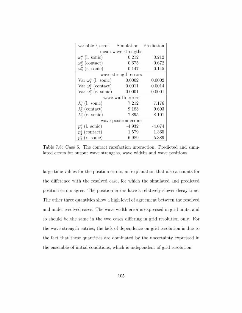
variable \ error Simulation Predictionmean wave strengths
ωo1 (l. sonic) 0.212 0.212
ωo2 (contact) 0.675 0.672
ωo3 (r. sonic) 0.147 0.145
wave strength errorsVar ωo
1 (l. sonic) 0.0002 0.0002Var ωo
2 (contact) 0.0011 0.0014Var ωo
3 (r. sonic) 0.0001 0.0001wave width errors
λo1 (l. sonic) 7.212 7.176
λo2 (contact) 9.183 9.693
λo3 (r. sonic) 7.895 8.101
wave position errorspo
1 (l. sonic) -4.932 -4.074po
2 (contact) 1.579 1.365po
3 (r. sonic) 6.989 5.389
Table 7.8: Case 5. The contact rarefaction interaction. Predicted and simu-lated errors for output wave strengths, wave widths and wave positions.
large time values for the position errors, an explanation that also accounts for
the difference with the resolved case, for which the simulated and predicted
position errors agree. The position errors have a relatively slower decay time.
The other three quantities show a high level of agreement between the resolved
and under resolved cases. The wave width error is expressed in grid units, and
so should be the same in the two cases differing in grid resolution only. For
the wave strength entries, the lack of dependence on grid resolution is due to
the fact that these quantities are dominated by the uncertainty expressed in
the ensemble of initial conditions, which is independent of grid resolution.
105

variable \ error Simulation Predictionmean wave strengths
ωo1 (l. sonic) 0.783 0.781
ωo2 (contact) 0.079 0.083
ωo3 (r. sonic) 0.015 0.017
wave strength errorsVar ωo
1 (l. sonic) 0.0016 0.0019Var ωo
2 (contact) 0.000001 0.000005Var ωo
3 (r. sonic) 0.00003 0.00004wave width errors
λo1 (l. sonic) 1.808 1.821
λo2 (contact) 3.947 4.248
wave position errorspo
1 (l. sonic) 0.678 0.427po
2 (contact) 0.797 0.589
Table 7.9: Case 6. The shock shock overtake. Predicted and simulated errorsfor output wave strengths, wave widths and wave positions.
variable \ error Simulation Predictionmean wave strengths
ωo1 (l. sonic) 0.138 0.139
wave strength errorsVar ωo
1 (l. sonic) 0.0001 0.0001wave width errors
λo1 (l. sonic) 8.183 6.662
wave position errorspo
1 (l. sonic) -5.957 -4.785
Table 7.10: Case 7. The crossing of two compressions. Predicted and simulatederrors for output wave strengths, wave widths and wave positions.
106
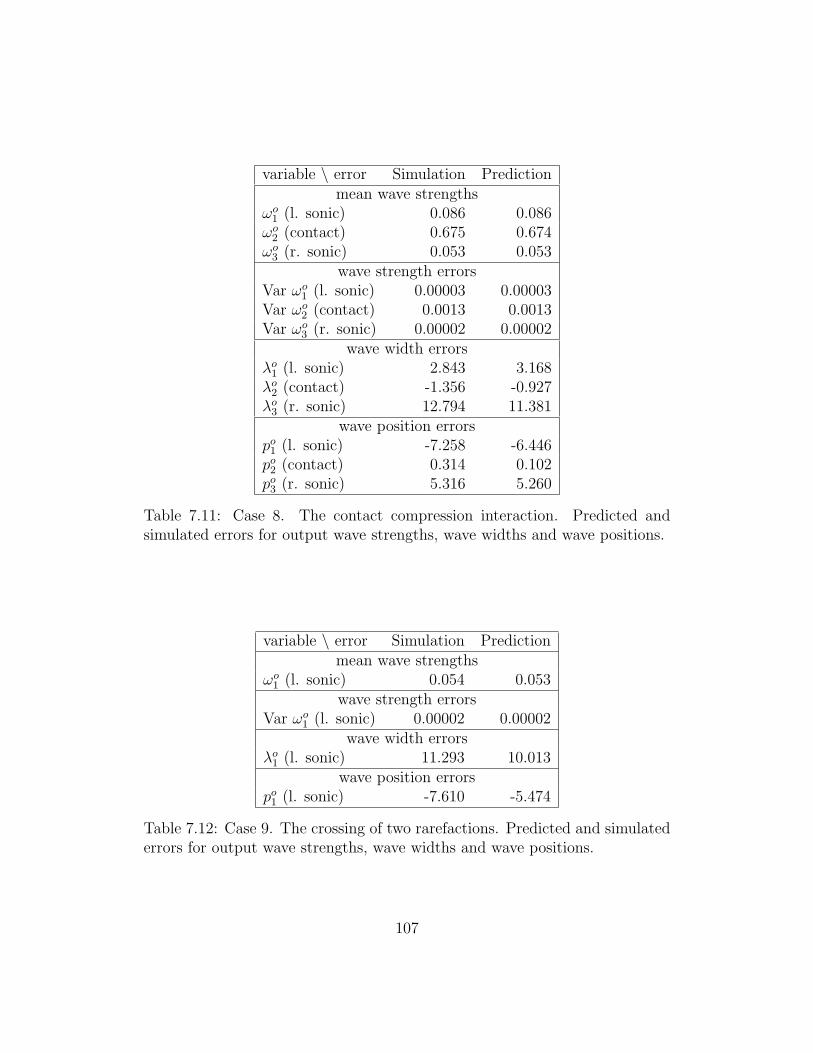
variable \ error Simulation Predictionmean wave strengths
ωo1 (l. sonic) 0.086 0.086
ωo2 (contact) 0.675 0.674
ωo3 (r. sonic) 0.053 0.053
wave strength errorsVar ωo
1 (l. sonic) 0.00003 0.00003Var ωo
2 (contact) 0.0013 0.0013Var ωo
3 (r. sonic) 0.00002 0.00002wave width errors
λo1 (l. sonic) 2.843 3.168
λo2 (contact) -1.356 -0.927
λo3 (r. sonic) 12.794 11.381
wave position errorspo
1 (l. sonic) -7.258 -6.446po
2 (contact) 0.314 0.102po
3 (r. sonic) 5.316 5.260
Table 7.11: Case 8. The contact compression interaction. Predicted andsimulated errors for output wave strengths, wave widths and wave positions.
variable \ error Simulation Predictionmean wave strengths
ωo1 (l. sonic) 0.054 0.053
wave strength errorsVar ωo
1 (l. sonic) 0.00002 0.00002wave width errors
λo1 (l. sonic) 11.293 10.013
wave position errorspo
1 (l. sonic) -7.610 -5.474
Table 7.12: Case 9. The crossing of two rarefactions. Predicted and simulatederrors for output wave strengths, wave widths and wave positions.
107

variable \ error Simulation Predictionmean wave strengths
ωo1 (l. sonic) 0.330 0.356
wave strength errorsVar ωo
1 (l. sonic) 0.0007 0.0002wave width errors
λo1 (l. sonic) 4.776 4.498
wave position errorspo
1 (l. sonic) 0.599 0.167
Table 7.13: Case 4. The crossing of two rarefactions. Predicted and simulatederrors for output wave strengths, wave widths and wave positions. Comparisonof under resolved simulation and prediction.
variable \ error Simulation Predictionmean wave strengths
ωo1 (l. sonic) 0.218 0.244
ωo2 (contact) 0.692 0.676
ωo3 (r. sonic) 0.142 0.157
wave strength errorsVar ωo
1 (l. sonic) 0.0002 0.0004Var ωo
2 (contact) 0.0009 0.0012Var ωo
3 (r. sonic) 0.0002 0.0003wave width errors
λo1 (l. sonic) 8.163 7.046
λo2 (contact) 9.775 10.408
λo3 (r. sonic) 7.042 7.584
wave position errorspo
1 (l. sonic) -8.997 -4.235po
2 (contact) 4.789 1.738po
3 (r. sonic) 7.198 4.284
Table 7.14: Case 5. The contact rarefaction interaction. Predicted and simu-lated errors for output wave strengths, wave widths and wave positions. Com-parison of under resolved simulation and prediction.
108
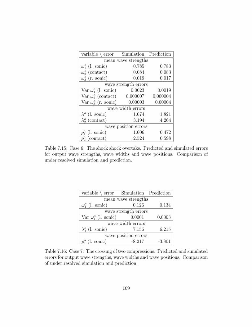
variable \ error Simulation Predictionmean wave strengths
ωo1 (l. sonic) 0.785 0.783
ωo2 (contact) 0.084 0.083
ωo3 (r. sonic) 0.019 0.017
wave strength errorsVar ωo
1 (l. sonic) 0.0023 0.0019Var ωo
2 (contact) 0.000007 0.000004Var ωo
3 (r. sonic) 0.00003 0.00004wave width errors
λo1 (l. sonic) 1.674 1.821
λo2 (contact) 3.194 4.264
wave position errorspo
1 (l. sonic) 1.606 0.472po
2 (contact) 2.524 0.598
Table 7.15: Case 6. The shock shock overtake. Predicted and simulated errorsfor output wave strengths, wave widths and wave positions. Comparison ofunder resolved simulation and prediction.
variable \ error Simulation Predictionmean wave strengths
ωo1 (l. sonic) 0.126 0.134
wave strength errorsVar ωo
1 (l. sonic) 0.0001 0.0003wave width errors
λo1 (l. sonic) 7.156 6.215
wave position errorspo
1 (l. sonic) -8.217 -3.801
Table 7.16: Case 7. The crossing of two compressions. Predicted and simulatederrors for output wave strengths, wave widths and wave positions. Comparisonof under resolved simulation and prediction.
109
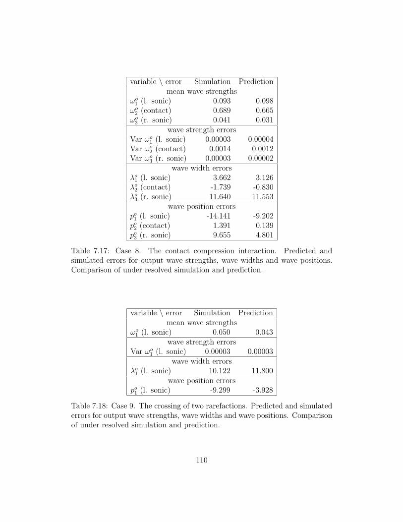
variable \ error Simulation Predictionmean wave strengths
ωo1 (l. sonic) 0.093 0.098
ωo2 (contact) 0.689 0.665
ωo3 (r. sonic) 0.041 0.031
wave strength errorsVar ωo
1 (l. sonic) 0.00003 0.00004Var ωo
2 (contact) 0.0014 0.0012Var ωo
3 (r. sonic) 0.00003 0.00002wave width errors
λo1 (l. sonic) 3.662 3.126
λo2 (contact) -1.739 -0.830
λo3 (r. sonic) 11.640 11.553
wave position errorspo
1 (l. sonic) -14.141 -9.202po
2 (contact) 1.391 0.139po
3 (r. sonic) 9.655 4.801
Table 7.17: Case 8. The contact compression interaction. Predicted andsimulated errors for output wave strengths, wave widths and wave positions.Comparison of under resolved simulation and prediction.
variable \ error Simulation Predictionmean wave strengths
ωo1 (l. sonic) 0.050 0.043
wave strength errorsVar ωo
1 (l. sonic) 0.00003 0.00003wave width errors
λo1 (l. sonic) 10.122 11.800
wave position errorspo
1 (l. sonic) -9.299 -3.928
Table 7.18: Case 9. The crossing of two rarefactions. Predicted and simulatederrors for output wave strengths, wave widths and wave positions. Comparisonof under resolved simulation and prediction.
110

Bibliography
[1] Natural Climate Variability on Decade-to-Century Time Scales. NationalAcademy Press, 1995.
[2] I. Babuska and W. Rheinboldt. A posteriori error estimates for the fi-nite element method. Internat. J. Numer. Methods Engrg., 12:1597–1615,1978.
[3] J. W. Barker, M. Cuypers, and L. Holden. Quantifying uncertainty inproduction forecasts: Another look at the PUNQ-S3 problem. TechnicalReport SPE 62925, 2000.
[4] G. Batchelor. The Theory of Homogeneous Turbulence. The UniversityPress, Cambridge, 1955.
[5] L. Bonet-Cunha, D. S. Oliver, R. A. Redner, and A. C. Reynolds. A hy-brid markov chair monte carlo method for generating permeability fieldsconditioned to multiwell pressure data and prior information. SPE Jour-nal, 3:261–271, 1998.
[6] A. Chorin and J. Marsden. A Mathematical Introduction to Fluid Mech-nics. Springer Verlag, New York–Heidelberg–Berlin, 2000.
[7] B. Cockburn and H. Gau. A posteriori error estimates of general numeri-cal methods for scalar conservation laws. Mat. Aplic. Comp., 14(1):37–47,1995.
[8] P. S. Craig, M. Goldstein, J. C. Rougier, and A. H. Seheult. Bayesianforecasting for complex systems using computer simulators. Journal OfThe American Statistical Association, 96:717–729, 2001.
[9] B. DeVolder, J. Glimm, J. W. Grove, Y. Kang, Y. Lee, K. Pao, D. H.Sharp, and K. Ye. Uncertainty quantification for multiscale simulations.Journal of Fluids Engineering, 124:29–41, 2002. LANL report No. LA-UR-01-4022.
111

[10] J. Glimm, J. W. Grove, Y. Kang, T. Lee, X. Li, D. H. Sharp, Y. Yu,K. Ye, and M. Zhao. Statistical riemann problems and a composition lawfor errors in numerical solutions of shock physics problems. SISC, 26:666–697, 2004. University at Stony Brook Preprint Number SB-AMS-03-11,Los Alamos National Laboratory number LA-UR-03-2921.
[11] J. Glimm, J. W. Grove, Y. Kang, T. Lee, X. Li, D. H. Sharp, Y. Yu, K. Ye,and M. Zhao. Errors in numerical solutions of spherically symmetricshock physics problems. Contemporary Mathematics, 371:163–179, 2005.University at Stony Brook Preprint Number SB-AMS-04-03, Los AlamosNational Laboratory number LA-UR-04-0713.
[12] J. Glimm, J. W. Grove, X. L. Li, W. Oh, and D. H. Sharp. A criticalanalysis of Rayleigh-Taylor growth rates. J. Comp. Phys., 169:652–677,2001.
[13] J. Glimm, J. W. Grove, X.-L. Li, K.-M. Shyue, Q. Zhang, and Y. Zeng.Three dimensional front tracking. SIAM J. Sci. Comp., 19:703–727, 1998.
[14] J. Glimm, J. W. Grove, X.-L. Li, and D. C. Tan. Robust computationalalgorithms for dynamic interface tracking in three dimensions. SIAM J.Sci. Comp., 21:2240–2256, 2000.
[15] J. Glimm, Yoon ha Lee, and Kenny Ye. A simple model for scale up error.Contemporary Mathematics, 295:241–251, 2002.
[16] J. Glimm, S. Hou, H. Kim, Y. Lee, D. Sharp, K. Ye, and Q. Zou.Risk management for petroleum reservoir production: A simulation-basedstudy of prediction. J. Comp. Geosciences, 5:173–197, 2001.
[17] J. Glimm, S. Hou, H. Kim, D. Sharp, and K. Ye. A probability model forerrors in the numerical solutions of a partial differential equation. CFDJournal, 9, 2000.
[18] J. Glimm, S. Hou, Y. Lee, D. Sharp, and K. Ye. Prediction of oil pro-duction with confidence intervals. SPE 66350, Society of Petroelum En-gineers, 2001. SPE Reservoir Simulation Symposium held in Houston,Texas, 11-14 Feb.
[19] J. Glimm and D. H. Sharp. Stochastic methods for the prediction ofcomplex multiscale phenomena. Quarterly J. Appl. Math., 56:741–765,1998.
112

[20] J. Glimm and D. H. Sharp. Prediction and the quantification of uncer-tainty. Physica D, 133:152–170, 1999.
[21] James Glimm, Yunha Lee, David H Sharp, and Kenny Q Ye. Predic-tion using numerical simulations, A Bayesian framework for uncertaintyquantification and its statistical challenge. In Bilal M. Ayyub and Nii O.Attoh-Okine, editors, Proceedings of the Fourth International Symposiumon Uncertainty Modeling and Analysis (ISUMA 2003). IEEE, ComputerSociety, 2003.
[22] G. Guderley. Starke kugelige und zylindrische verdichtungsstosse in derNahe des kugelmittelpuktes bzw der zylinderachse. Luftfahrtforschung,19:302–312, 1942.
[23] A. Harten. ENO schemes with subcell resolution. J. Comp. Phys.,83:148–184, 1989.
[24] B. K. Hegstad and H. Omre. Uncertainty assessment in history matchingand forecasting. In E. Y. Baafi and N. A. Schofield, editors, GeostatisticsWollongong ’96, pages 585–596. Kluwer Academic Publishers, 1997.
[25] Yunghee Kang. Estimation of Computational Simulation Errors in GasDynamics. PhD thesis, State Univ. of New York at Stony Brook, 2003.LANL Report LA-UR-03-2700.
[26] M. C. Kennedy and A. O’Hagan. Bayesian calibration of computer mod-els. Journal Of The Royal Statistical Society Series B-Statistical Method-ology, 63(3):425–450, 2001.
[27] L. Lake. Enhanced Oil Recovery. Prentice-Hall, Englewood Cliffs, 1989.
[28] L. Machiels, A. Patera, J. Peraire, and Y. Maday. A general frameworkfor finite element a posteriori error control: Application to linear and non-linear convection-dominated problems. In Proceedings ICFD Conferenceon Numerical Methods for Fluid Dynamics, Oxford, England, March 31 -April 3. 1998.
[29] W. D. McComb. The Physics of Fluid Turbulence. Oxford UniversityPress, Oxford, 1990.
[30] J. C. Niemeyer and W. Hillebrandt. Turbulent nuclear flames in Type Iasupernovae. ApJ, 452:769–778, 1995.
113

[31] J. T. Oden and M. Ainsworth. A Posteriori Error Estimation in FiniteElement Analysis. John Wiley & Sons, New York, 2000.
[32] W. Press, S. Teukolsky, W. Vetterling, and B. Flannery. NumericalRecipes in Fortran 77. Cambridge University Press, 1992.
[33] R. Richtmyer and K. Morton. Difference Methods for Initial Value Prob-lems. Interscience, New York, second edition, 1967.
[34] D. H. Sharp. An overview of Rayleigh-Taylor instability. Physica D,12:3–18, 1984.
[35] J. Smoller. Shock Waves and Reaction-Diffusion Equations. Springer-Verlag, New York, 1983.
[36] G. B. Whitham. Linear and Nonlinear Waves. John Wiley & Sons, NewYork, 1974.
114
Top Related