


Languages
Pages
Legal

1
iisrVdtbtta
optltbcscsod
srpelapgsvOsbwmi
p
J
Downlo
Russell Trahan IIIe-mail: [email protected]
Tamás Kalmár-Nagye-mail: [email protected]
Department of Aerospace Engineering,Texas A&M University,
College Station, TX 77843
Equilibrium, Stability, andDynamics of RectangularLiquid-Filled VesselsHere we focus on the stability and dynamic characteristics of a rectangular, liquid-filledvessel. The position vector of the center of gravity of the liquid volume is derived andused to express the equilibrium angles of the vessel. Analysis of the potential functiondetermines the stability of these equilibria, and bifurcation diagrams are constructed todemonstrate the co-existence of several equilibrium configurations of the vessel. To vali-date the results, a vessel of rectangular cross section was built. The results of the experi-ments agree well with the theoretical predictions of stability. The dynamics of the un-forced and forced systems with a threshold constraint is discussed in the context of thenonlinear Mathieu equation. �DOI: 10.1115/1.4003915�
IntroductionDetermining equilibrium positions of structures and character-
zing their stability is a common engineering task. Fluid-structurenteractions are one of the many stability concerns in dynamicystems. For example, some marine structures such as floating oiligs and dry-docks use water as ballast to stabilize the structure.ehicles such as aircraft, boats, and machinery operate under con-itions where the fuel tank or liquid payload may adversely affecthe stability of the vehicle due to sloshing �1�. Determining theehavior of the liquid in a tank is an important consideration inhe design and analysis of these devices. These examples providehe motivation for our stability analysis and dynamic modeling ofrectangular liquid-filled vessel.This paper discusses the static stability and simplified equation
f motion of a vessel with a rectangular cross section that canivot about a fixed point and contains liquid. The emphasis withhe equation of motion is the state constraint representative of theiquid spilling from the vessel. An equally important purpose forhis paper is to present an example through which the concepts ofifurcations, potential functions, and stability of nonlinear physi-al systems become more available to students. The experimentaletup described here is easy to build and may serve as an effectivelassroom demonstration. A similar system—a hanging block—istudied by Stépán and Bianchi �2�. They characterized the stabilityf a mass hanging from two ropes by using a potential functionepending on various geometric parameters of the system.
Research into the stability of floating bodies has a long history,tarting with Archimedes’ On Floating Bodies. The ship problemelates the buoyancy force to ship stability. Locating equilibriumositions of floating objects and ascertaining the stability of thesequilibria is not a trivial exercise. Duffy �3� considered the equi-ibrium positions of partially submerged rods supported at one endnd showed the existence of simple bifurcations and the jumphenomenon �hysteresis� in the problem. Erdös et al. �4� investi-ated the equilibrium configurations for floating solid prisms ofquare and equilateral triangular cross section. Delbourgo �5� pro-ided a solution to the metacentric problem for a floating plank.ur system can be thought of as an inverted ship problem �for the
hip problem, the body is submerged in the liquid�. While Del-ourgo’s problem is analogous to ours and his results are similar,e believe that our exposition is more detailed and lucid, therebyaking this type of problem more known to the nonlinear dynam-
cs community.
Manuscript received May 28, 2010; final manuscript received March 31, 2011;
ublished online May 20, 2011. Assoc. Editor: Bala Balachandran.ournal of Computational and Nonlinear DynamicsCopyright © 20
aded 24 Jun 2011 to 165.91.74.118. Redistribution subject to ASME
We start by defining the geometry of the vessel and the liquidcontained within in Sec. 2. The physical parameters that are variedare the amount of liquid, the pivot height to vessel-width ratio,and the angle of rotation about the pivot. The algebraic equationsdescribing the location of the center of gravity of the liquid arederived. From these equations, the equilibrium positions of thevessel are expressed in Sec. 3. The stability of the equilibriumpositions is determined with a potential function in Sec. 3.2. Theresults from the equilibrium calculations and stability analysis areused to construct bifurcation diagrams for various physical param-eters of the vessel in Sec. 4. These diagrams are then comparedwith experimental data in Sec. 5. Lastly a simplified equation ofmotion is presented in Sec. 6. The response of the system and thestate constraint are discussed in Sec.7.
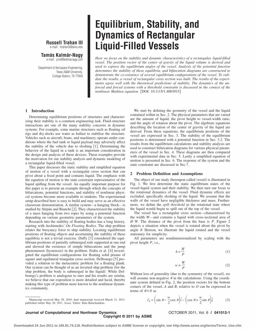
2 Problem Definition and AssumptionsThe object of our study �hereupon called vessel� is illustrated in
Fig. 1. We first determine the static equilibrium states of thevessel-liquid system and their stability. We then turn our focus tothe rotational dynamics of the vessel. Fluid dynamic effects areexcluded, specifically sloshing of the liquid. We assume that thewalls of the vessel have negligible thickness and mass. Further-more, we define the spill threshold as the rotational state wherethe liquid would begin to spill out of the top of the vessel.
The vessel has a rectangular cross section—characterized bythe width W—and contains a liquid with cross-sectional area ofH ·W. The distance of the pivot from the base is P. Figure 2depicts a situation when the vessel is rotated about the pivot byangle �. Hereon, we illustrate the liquid rotated and the vesselstationary for simplicity.
All parameters are nondimensionalized by scaling with thepivot height P, i.e.,
h =H
P�1�
w =W
P�2�
Without loss of generality �due to the symmetry of the vessel�, wewill assume non-negative � in the calculations. Using the coordi-nate system defined in Fig. 2, the position vectors for the bottomcorners of the vessel, A and B, relative to O can be expressed interms of ��0 as
r�A = �sin � −w
cos �� i − �cos � +w
sin �� j �3�
2 2OCTOBER 2011, Vol. 6 / 041012-111 by ASME
license or copyright; see http://www.asme.org/terms/Terms_Use.cfm
Tc
ivtr
aa
Ev
0
Downlo
r�B = �sin � +w
2cos �� i − �cos � +
w
2sin �� j �4�
hese expressions will later be used to derive the location of theenter of gravity �CG� of the liquid cross section.
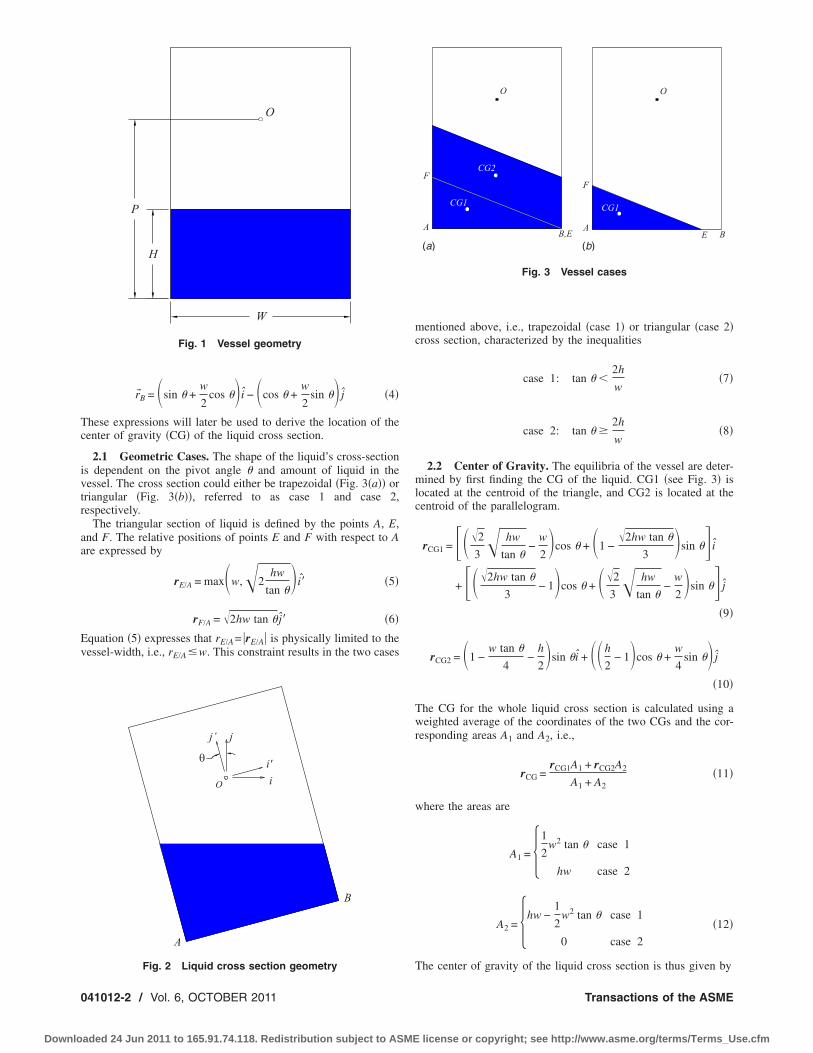
2.1 Geometric Cases. The shape of the liquid’s cross-sections dependent on the pivot angle � and amount of liquid in theessel. The cross section could either be trapezoidal �Fig. 3�a�� orriangular �Fig. 3�b��, referred to as case 1 and case 2,espectively.
The triangular section of liquid is defined by the points A, E,nd F. The relative positions of points E and F with respect to Are expressed by
rE/A = max�w,�2hw
tan ��i� �5�
rF/A = �2hw tan � j� �6�
quation �5� expresses that rE/A= �rE/A� is physically limited to theessel-width, i.e., rE/A�w. This constraint results in the two cases
O
j’ j
i
i'�
A
B
O
P
H
W
Fig. 1 Vessel geometry
Fig. 2 Liquid cross section geometry
41012-2 / Vol. 6, OCTOBER 2011
aded 24 Jun 2011 to 165.91.74.118. Redistribution subject to ASME
mentioned above, i.e., trapezoidal �case 1� or triangular �case 2�cross section, characterized by the inequalities
case 1: tan � �2h
w�7�
case 2: tan � �2h
w�8�
2.2 Center of Gravity. The equilibria of the vessel are deter-mined by first finding the CG of the liquid. CG1 �see Fig. 3� islocated at the centroid of the triangle, and CG2 is located at thecentroid of the parallelogram.
rCG1 = ��2
3� hw
tan �−
w
2�cos � + �1 −
�2hw tan �
3�sin � i
+ ��2hw tan �
3− 1�cos � + ��2
3� hw
tan �−
w
2�sin � j
�9�
rCG2 = �1 −w tan �
4−
h
2�sin �i + ��h
2− 1�cos � +
w
4sin �� j
�10�
The CG for the whole liquid cross section is calculated using aweighted average of the coordinates of the two CGs and the cor-responding areas A1 and A2, i.e.,
rCG =rCG1A1 + rCG2A2
A1 + A2�11�
where the areas are
A1 = �1
2w2 tan � case 1
hw case 2�
A2 = �hw −1
2w2 tan � case 1
0 case 2� �12�
(a)
O
F
AB,E
CG2
CG1
O
F
AE
CG1
B
(b)
Fig. 3 Vessel cases
The center of gravity of the liquid cross section is thus given by
Transactions of the ASME
license or copyright; see http://www.asme.org/terms/Terms_Use.cfm

3
td
U
Ps
ro
If
ear
sn
J
Downlo
rCG = ��1 −w2 tan2 �
24h−
w2
12h−
h
2�sin �i + ��h
2− 1�cos � +
w2 tan � sin �
24h� j case 1
��2
3� hw
tan �−
w
2�cos � + �1 −
�2hw tan �
3�sin � i + ��2hw tan �
3− 1�cos � + ��2
3� hw
tan �−
w
2�sin � j case 2�
�13�
Potential Function, Equilibria, and StabilityThe equilibrium angles of the vessel and their stability are de-
ermined by analyzing the nondimensional potential function �6�efined by the j component of the CG location:
rCG · j
= � �h
2− 1�cos � −
w2 tan � sin �
24hcase 1
��2hw tan �
3− 1�cos � + ��2
3� hw
tan �−
w
2�sin � case 2�
�14�hysically, the vessel is in equilibrium when the CG of the crossection of the liquid is on the vertical axis. This is expressed as
CG· i=0 It is also true that rCG· i=0 corresponds to local extremaf the potential function, i.e.,
dU
d�= 0 = � �1 −
w2 tan2 �
24h−
w2
12h−
h
2�sin � case 1
�2hw
3−
w
2tan1/2 � + tan3/2 � −
�2hw
3tan2 � case 2�
�15�n Sec. 3.2, we will use the second derivative of the potentialunction to classify the stability of particular equilibria.
3.1 Equilibria Conditions. Plotted in Fig. 4 are the nonzeroquilibrium positions given by Eq. �15� in h−w−� space. The leftnd right shaded regions depict case 2 and case 1 equilibria,espectively.
As can be observed, for given values of h and w, multiple �olutions can exist. We now define the domains in which differentumbers of equilibria exist.
Case 1 equilibria are determined by �see Eq. �15��
0°
20°
0.0
0.040°
0.5
0.5�
1.0
1.0
60°
1.5
1.5
2.0
80°
2.5
2.0
3.0
90°h
w
Fig. 4 h−w−� plot of �Å0 equilibria
ournal of Computational and Nonlinear Dynamics
aded 24 Jun 2011 to 165.91.74.118. Redistribution subject to ASME
�1 −w2 tan2 �
24h−
w2
12h−
h
2�sin � = 0, 0 � tan � �
2h
w�16�
Clearly, �=0 is always a solution. Other solutions satisfy
tan2 � = �2h − h2�12
w2 − 2, 0 � tan � �2h
w�17�
Expression �17� is equivalent to the two inequalities:
�h − 1�2 +w2
6� 1 �18�
�h −3
4�2
+w2
8�
9
16�19�
which determine that a positive � solution exists between the twohalf-ellipses shown in Fig. 5. For later reference, we refer to equa-tion �h− �3 /4��2+ �w2 /8�= �9 /16� as curve I.
Case 2 equilibria are given by
�2hw
3−
w
2tan1/2 � + tan3/2 � −
�2hw
3tan2 � = 0 �20�
subject to the constraint
tan � �2h
w�21�
It can be shown that Eq. �20� has three non-negative roots. Theregions in h-w space with one or three real roots are separated bya curve on which Eq. �20� has a double root. For Eq. �20� to havea double root it is necessary that its derivative vanishes, i.e.,
− 3w + 18 tan � − 8�2�hw tan3/2 � = 0. �22�
Equations �20� and �22� are now combined and solved for h and wto give the boundary in parametric form in terms of � as
h0 0.5 1 1.5 2
w
0
0.5
1
1.5
2
1 solution
0 solutions
0 solutions
I
Fig. 5 Number of solutions of expression „17…
OCTOBER 2011, Vol. 6 / 041012-3
license or copyright; see http://www.asme.org/terms/Terms_Use.cfm

Ttt
w
Opt
ltss=
rm
0
Downlo
h��� =9 tan2 �
�tan2 � + 3��3 tan2 � + 1��23�
w��� =2 tan ��tan2 � + 3�
3 tan2 � + 1�24�
he parametric curve �h��� ,w����, referred to as curve II, is plot-ed in Fig. 6. The region left of the curve is where Eq. �20� hashree real roots.1
Substituting the constraint �21� into Eq. �20� gives
− 12h3/2�w + 8h5/2�w + �hw5/2 � 0 �25�hich can also be expressed as
�h −3
4�2
+w2
8�
9
16�26�
utside of this elliptical region �bounded by curve I�, one of theossible real roots does not satisfy constraint �21�. Figure 7 showshe number of valid case 2 solutions in the h-w plane.
We are now in a position to present information about all equi-ibria of the vessel. Recall that in the calculations � was assumedo be non-negative. Without this restriction each case 1 and case 2olution corresponds to two equilibrium configurations of the ves-el, resulting in an odd number of equilibria for the system ��0, case 1, and case 2 equilibria�. Figure 8 shows the various
1This statement can be proved by considering the h=0, w=2 case. Equation �20�educes to tan3 �−tan �=0, which clearly has three real roots. By a continuity argu-ent, Eq. �20� has three real roots in the region left of the double root curve.
1
h
w
3 roots
1 root2 roots
Cusp (9/16, 2)
II
Fig. 6 Number of real roots in Eq. „20…
41012-4 / Vol. 6, OCTOBER 2011
aded 24 Jun 2011 to 165.91.74.118. Redistribution subject to ASME
regions and indicates the total number of equilibria. The grayregion is where case 2 equilibria are present.
3.2 Stability Conditions. An equilibrium position is stable orunstable if the second derivative of the potential function evalu-ated at the equilibrium is positive or negative, respectively �cor-responding to a local minimum or maximum of the potential func-tion� �6�. The second derivative of the potential function �14� is
2solu
tions
1 solution
3 solutions
0 solutions
1
h
w
Fig. 7 Number of solutions in Eq. „20… with constraint „21…
5eq
uil
ibri
a
3 equilibria
3 equilibria
1 equilibrium
h
w
7 equilibria
I
II
Fig. 8 Total number of equilibria for the vessel in terms of hand w. Solid lines demarcate regions with different numbers ofequilibria. The shaded region refers to the validity domain ofcase 2.
d2U
d�2 = ��1 −h
2�cos � −
w2
24h�2 cos � + 3 sin2 � cos−1 � + 2 sin4 � cos−3 �� case 1
−�2hw
6�sin5/2 � cos−3/2 � + 6 sin1/2 � cos1/2 � + sin−3/2 � cos5/2 �� + cos � +
w
2sin � case 2� �27�
Transactions of the ASME
license or copyright; see http://www.asme.org/terms/Terms_Use.cfm
Tf
Tb�topts
al�
4
tcSatv
edt
p
btt8ps1
eq
J
Downlo
he stability condition for �=0 assumes a particularly simpleorm
�d2U
d�2 ��=0
= 1 −h
2−
w2
12h� 0 �28�
�h − 1�2 +w2
6� 1 �29�
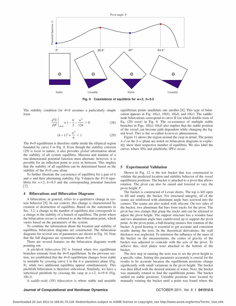
he �=0 equilibrium is therefore stable inside the elliptical regionounded by curve I in Fig. 8. Even though the stability criterion29� is local in nature, it also provides global information abouthe stability of all system equilibria. Maxima and minima of ane-dimensional potential function must alternate; however, it isossible for an inflection point to exist in between. This implieshat the stability of all equilibria can be determined based on thetability of the �=0 case alone.
To further illustrate the coexistence of equilibria for a pair of hnd w and their alternating stability, Fig. 9 depicts the ��0 equi-ibria for w=2, h=0.5 and the corresponding potential function7�.
Bifurcations and Bifurcation DiagramsA bifurcation, in general, refers to a qualitative change in sys-
em behavior �8�. In our context, this change is characterized byreation or destruction of equilibria. Based on the statements inec. 3.2, a change in the number of equilibria also corresponds tochange in the stability of a branch of equilibria. The point where
he bifurcation occurs is referred to as the bifurcation point, whicharies based on the parameters of the system.
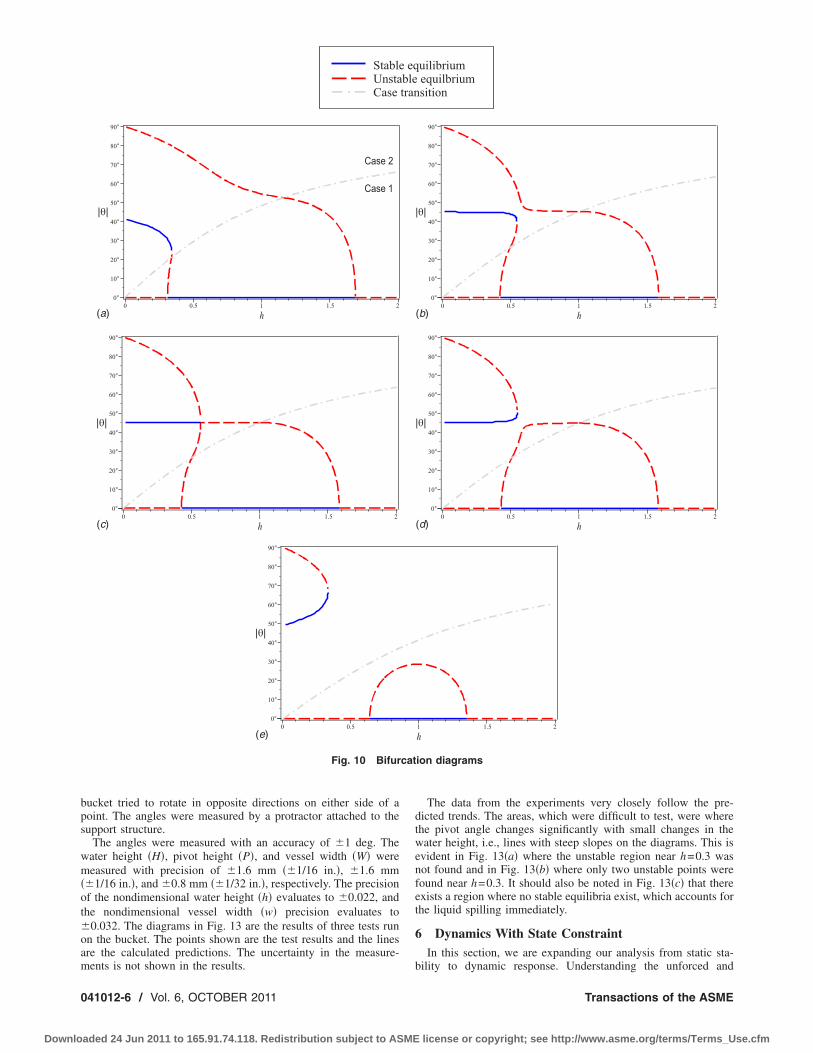
To combine the information about the location and stability ofquilibria, bifurcation diagrams are constructed. The bifurcationiagrams for several sets of parameters are shown in Fig. 10. Notehat the full diagrams are symmetric about �=0.
There are several features on the bifurcation diagrams worthointing out.
A pitchfork bifurcation �9� is formed when two equilibriumranches emanate from the �=0 equilibrium. In the previous sec-ion, we established that the �=0 equilibrium changes from stableo unstable by crossing curve I in the h-w parameter plane �Fig.�, while two additional equilibria appear simultaneously. Thisitchfork bifurcation is therefore subcritical. Similarly, we have aubcritical pitchfork by crossing the cusp at w=2, h=9 /6 �Fig.0�c��.
0° 26.5°
Stable Unstable
Pivot
Pote
nti
alfu
nct
ion:
U
Fig. 9 Coexistence of
A saddle-node (SN) bifurcation is where stable and unstable
ournal of Computational and Nonlinear Dynamics
aded 24 Jun 2011 to 165.91.74.118. Redistribution subject to ASME
equilibrium points annihilate one another �8�. This type of bifur-cation appears in Fig. 10�a�, 10�b�, 10�d�, and 10�e�. The saddle-node bifurcations correspond to curve II �on which double roots ofEq. �20� exist� in Fig. 8. The co-existence of multiple stablebranches in Figs. 10�a�–10�d� also implies that the stable positionof the vessel can become path dependent while changing the liq-uid level. This is the so-called hysteresis phenomenon.
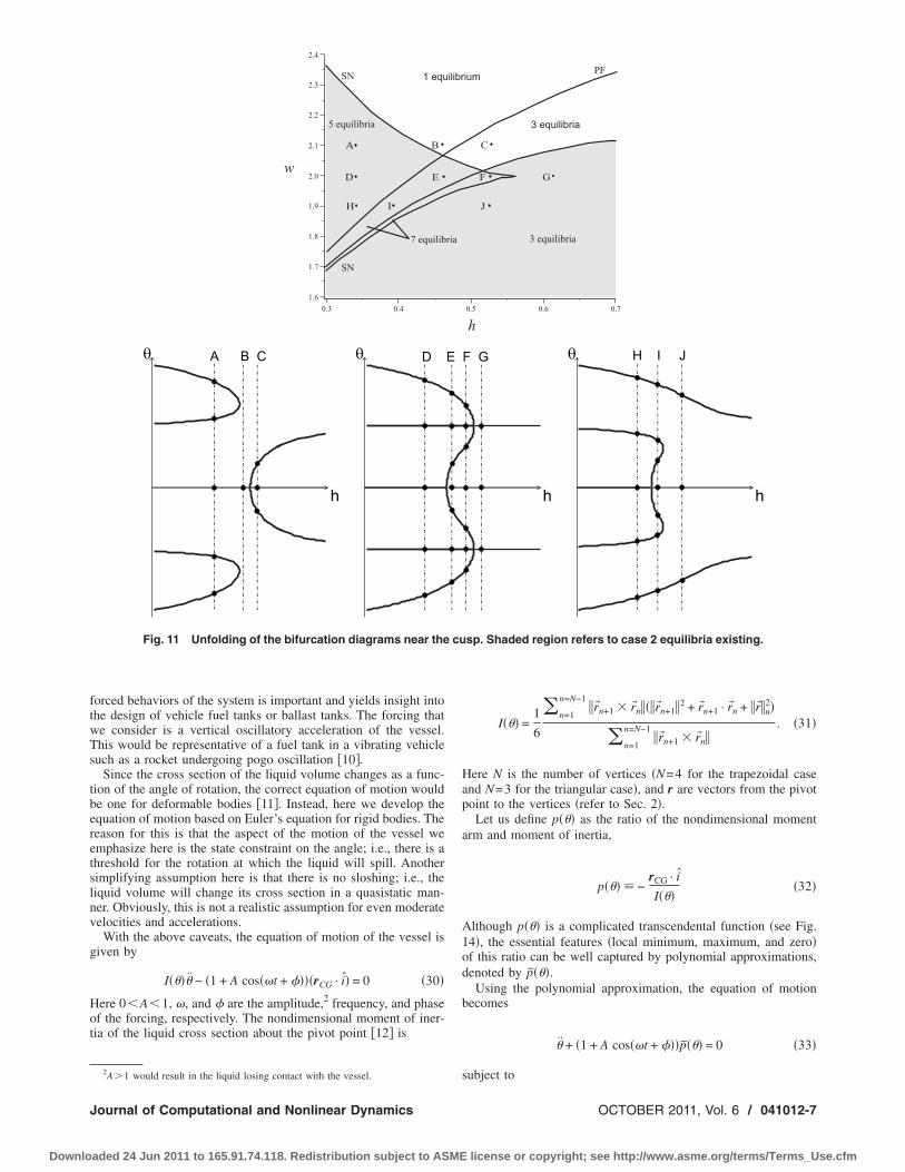
Figure 11 shows the region around the cusp in detail. The pointsA-J on the h-w plane are noted on bifurcation diagrams to explic-itly show their respective number of equilibria. We also label thecurves where SNs and pitchforks �PFs� occur.
5 Experimental ValidationShown in Fig. 12 is the test bucket that was constructed to
validate the predicted location and stability behavior of the vesselequilibrium positions. The bucket is attached to a pivot that allowsrotation. The pivot can also be raised and lowered to vary thepivot height P.
The bucket is constructed of Lexan sheets. The top is left opento fill and empty the bucket. For structural integrity, all of theseams are reinforced with aluminum angle bars screwed into thecorners. The seams are also sealed with silicone. On two sides ofthe bucket, two aluminum flat bars form tracks for the pivot. Thepivot has two clamps that grasp the tracks and can be released toadjust the pivot height. The support structure has a wooden baseand two aluminum angle bars cantilevered up to support the pivotpoint. At the pivot point, a ball-bearing ensures free rotation of thebucket. A good bearing is essential to get accurate and consistentresults during the tests. In the theoretical derivations, the wallthickness was neglected. To minimize the influence of the mass ofthe bucket on the measurements, the center of gravity of thebucket was adjusted to coincide with the axis of the pivot. Toachieve this, steel plates were attached to the bottom of thebucket.
The first step in running the tests was to set the pivot height toa specific value. Setting this parameter accurately is crucial for theresults to be accurate because the equilibrium positions changesignificantly with small variations in the pivot height. The bucketwas then filled with the desired amount of water. Next, the bucketwas manually rotated to find the equilibrium points. The bucketsettled on stable positions. Unstable positions were located by
45° 63.4°
Stable Unstable
le: �
uilibria for w=2, h=0.5
ang
manually rotating the bucket until a point was found where the
OCTOBER 2011, Vol. 6 / 041012-5
license or copyright; see http://www.asme.org/terms/Terms_Use.cfm
bps
wm�ot�oam
0
Downlo
ucket tried to rotate in opposite directions on either side of aoint. The angles were measured by a protractor attached to theupport structure.
The angles were measured with an accuracy of �1 deg. Theater height �H�, pivot height �P�, and vessel width �W� wereeasured with precision of �1.6 mm ��1/16 in.�, �1.6 mm
�1/16 in.�, and �0.8 mm ��1/32 in.�, respectively. The precisionf the nondimensional water height �h� evaluates to �0.022, andhe nondimensional vessel width �w� precision evaluates to
0.032. The diagrams in Fig. 13 are the results of three tests runn the bucket. The points shown are the test results and the linesre the calculated predictions. The uncertainty in the measure-
h0 0.5 1 1.5 2
| |�
Case 2
Case 1
0°
10°
20°
30°
40°
50°
60°
70°
80°
90°
(a)
0 0.5 1 1.5 2
h
| |�
0°
10°
20°
30°
40°
50°
60°
70°
80°
90°
(c)
0 0.5
0°
10°
20°
30°
40°
50°
60°
70°
80°
90°
| |�
(e)
StableUnstaCase
Fig. 10 Bifur
ents is not shown in the results.
41012-6 / Vol. 6, OCTOBER 2011
aded 24 Jun 2011 to 165.91.74.118. Redistribution subject to ASME
The data from the experiments very closely follow the pre-dicted trends. The areas, which were difficult to test, were wherethe pivot angle changes significantly with small changes in thewater height, i.e., lines with steep slopes on the diagrams. This isevident in Fig. 13�a� where the unstable region near h=0.3 wasnot found and in Fig. 13�b� where only two unstable points werefound near h=0.3. It should also be noted in Fig. 13�c� that thereexists a region where no stable equilibria exist, which accounts forthe liquid spilling immediately.
6 Dynamics With State ConstraintIn this section, we are expanding our analysis from static sta-
0 0.5 1 1.5 2
h
| |�
0°
10°
20°
30°
40°
50°
60°
70°
80°
90°
(b)
0 0.5 1 1.5 2
h
| |�
0°
10°
20°
30°
40°
50°
60°
70°
80°
90°
(d)
1 1.5 2
h
uilibriumequilbriumsition
ion diagrams
eqbletran
cat
bility to dynamic response. Understanding the unforced and
Transactions of the ASME
license or copyright; see http://www.asme.org/terms/Terms_Use.cfm
ftwTs
tberetslnv
g
Hot
J
Downlo
orced behaviors of the system is important and yields insight intohe design of vehicle fuel tanks or ballast tanks. The forcing thate consider is a vertical oscillatory acceleration of the vessel.his would be representative of a fuel tank in a vibrating vehicleuch as a rocket undergoing pogo oscillation �10�.
Since the cross section of the liquid volume changes as a func-ion of the angle of rotation, the correct equation of motion woulde one for deformable bodies �11�. Instead, here we develop thequation of motion based on Euler’s equation for rigid bodies. Theeason for this is that the aspect of the motion of the vessel wemphasize here is the state constraint on the angle; i.e., there is ahreshold for the rotation at which the liquid will spill. Anotherimplifying assumption here is that there is no sloshing; i.e., theiquid volume will change its cross section in a quasistatic man-er. Obviously, this is not a realistic assumption for even moderateelocities and accelerations.
With the above caveats, the equation of motion of the vessel isiven by
I���� − �1 + A cos��t + ����rCG · i� = 0 �30�
ere 0�A�1, �, and � are the amplitude,2 frequency, and phasef the forcing, respectively. The nondimensional moment of iner-ia of the liquid cross section about the pivot point �12� is
2
0.3 0.4
1.6
1.7
1.8
1.9
2.0
2.1
2.2
2.3
2.4
1 equ
5 equilibria
D E
A B
H I
7 equilib
w
SN
SN
Fig. 11 Unfolding of the bifurcation diagrams near the
A�1 would result in the liquid losing contact with the vessel.
ournal of Computational and Nonlinear Dynamics
aded 24 Jun 2011 to 165.91.74.118. Redistribution subject to ASME
I��� =1
6
�n=1
n=N−1�r�n+1 r�n���r�n+1�2 + r�n+1 · r�n + �r��n
2�
�n=1
n=N−1�r�n+1 r�n�
. �31�
Here N is the number of vertices �N=4 for the trapezoidal caseand N=3 for the triangular case�, and r are vectors from the pivotpoint to the vertices �refer to Sec. 2�.
Let us define p��� as the ratio of the nondimensional momentarm and moment of inertia,
p��� −rCG · i
I����32�
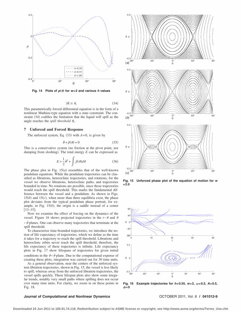
Although p��� is a complicated transcendental function �see Fig.14�, the essential features �local minimum, maximum, and zero�of this ratio can be well captured by polynomial approximations,denoted by p���.
Using the polynomial approximation, the equation of motionbecomes
� + �1 + A cos��t + ���p��� = 0 �33�
0.5 0.6 0.7
ium
3 equilibria
3 equilibria
F G
C
J
h
PF
sp. Shaded region refers to case 2 equilibria existing.
ilibr
ria
cu
subject to
OCTOBER 2011, Vol. 6 / 041012-7
license or copyright; see http://www.asme.org/terms/Terms_Use.cfm

0
Downlo
(a)
203.2mm (8”)
40
6.4
mm
(16
”)
Support structure
Ball-bearing pivot
Pivot track
Bucket
Protractor
(b)
Fig. 12 Test bucket design and apparatus
0 0.5 1 1.5 2
h
| |�
0°
10°
20°
30°
40°
50°
60°
70°
80°
90°
(a)0 0.5 1 1.5 2
| |�
0°
10°
20°
30°
40°
50°
60°
70°
80°
90°
h(b)
0 0.5 1 1.5 2
| |�
0°
10°
20°
30°
40°
50°
60°
70°
80°
90°
h(c)
Stable PredictionUnstable PredictionExperimental StableExperimental Unstable
Fig. 13 Experimental results
41012-8 / Vol. 6, OCTOBER 2011 Transactions of the ASME
aded 24 Jun 2011 to 165.91.74.118. Redistribution subject to ASME license or copyright; see http://www.asme.org/terms/Terms_Use.cfm
Tnsa
7
Td
Tpsvbwf1pa�
v
−s
tihlp
cc
ttvloF
=2.0
J
Downlo
��� � �t �34�
his parametrically forced differential equation is in the form of aonlinear Mathieu-type equation with a state constraint. The con-traint �34� codifies the limitation that the liquid will spill as thengle reaches the spill threshold �t.
Unforced and Forced ResponseThe unforced system, Eq. �33� with A=0, is given by
� + p��� = 0 �35�his is a conservative system �no friction at the pivot point, noramping from sloshing�. The total energy E can be expressed as
E =1
2�2 +� p���d� �36�
he phase plot in Fig. 15�a� resembles that of the well-knownendulum equations. While the pendulum trajectories can be clas-ified as librations, heteroclinic trajectories, and rotations, for theessel we observe librations, heteroclinic paths, and trajectoriesounded in time. No rotations are possible, since those trajectoriesould reach the spill threshold. This marks the fundamental dif-
erence between the vessel and a pendulum. As shown in Figs.5�b� and 15�c�, when more than three equilibria exist, the phaselot deviates from the typical pendulum phase portrait, for ex-mple, in Fig. 15�b�, the origin is a saddle instead of a center13–15�.
Now we examine the effect of forcing on the dynamics of theessel. Figure 16 shows projected trajectories in the t−� and �
� planes. One can observe many trajectories that terminate at thepill threshold.
To characterize time-bounded trajectories, we introduce the no-ion of life expectancy of trajectories, which we define as the timet takes for a trajectory to reach the spill threshold. Librations andeteroclinic orbits never reach the spill threshold; therefore, theife expectancy of these trajectories is infinite. Life expectancylots in Fig. 17 show lifespans of trajectories for given initial
onditions in the �− � plane. Due to the computational expense ofreating these plots, integration was carried out for 30 time units.
As a general observation, near the centers of the unforced sys-em libration trajectories, shown in Fig. 15, the vessel is less likelyo spill, whereas away from the unforced libration trajectories, theessel spills quickly. These lifespan plots also show some irregu-ar trends, notably very small paths where spilling does not occurver many time units. For clarity, we zoom in on these points in
�0° 30° 60° 90°
-0.4
-0.2
0
0.2
h=0.20
h=0.55
h=1.00
p
Fig. 14 Plots of p„�… for w=2 and various h values
ig. 18.
ournal of Computational and Nonlinear Dynamics
aded 24 Jun 2011 to 165.91.74.118. Redistribution subject to ASME
-90° -45° 0° 45° 90°
-0.3
0
0.3
�
��
(a)
-90° -45° 0° 45° 90°
-0.3
0
0.3
�
��
(b)
-90° -45° 0° 45° 90°
-0.2
0
0.2
�
��
(c)
Fig. 15 Unforced phase plot of the equation of motion for w
0 15 30 45 60
-90°
-45°
0°
45°
90°
t
-90° -60° -30° 0° 30° 60° 90°
-0.3
0
0.3
�
��
�
Fig. 16 Example trajectories for h=0.55, w=2, �=0.5, A=0.5,
�=0OCTOBER 2011, Vol. 6 / 041012-9
license or copyright; see http://www.asme.org/terms/Terms_Use.cfm

0
Downlo
-90° -60° -30° 0° 30° 60° 90°-0.25
-0.125
0
0.125
0.25
�
��
(a)-90° -60° -30° 0° 30° 60° 90°
-0.25
-0.125
0
0.125
0.25
�
��
(b)
-90° -60° -30° 0° 30° 60° 90°-0.25
-0.125
0
0.125
0.25
�
��
(c)-90° -60° -30° 0° 30° 60° 90°
-0.25
-0.125
0
0.125
0.25
�
��
(d)
0 15 30
Time to spill
Fig. 17 Lifespan of trajectories for various initial conditions, amplitudes, and frequencies for h=0.55 and w=2. The color
scale denotes the lifespan in time units.0 15 30Time to spill
-90° -60° -30° 0° 30° 60° 90°-0.25
-0.125
0
0.125
0.25
�
��
(a)0° 10° 20° 30°
0.0625
0.125
0.1875
�
��
(b)
24.5° 25° 25.5° 26°0.075
0.078
0.08
�
��
(c)0 15 30 45 60
-90˚
-45˚
0˚
45˚
90˚
t
�
Initial �
24.7524.9024.95
(d)
Fig. 18 Zooming in on the lifespan plot for �=0.75, A=0.75, �=0. The three initial conditions for „d… are marked on „c….
41012-10 / Vol. 6, OCTOBER 2011 Transactions of the ASME
aded 24 Jun 2011 to 165.91.74.118. Redistribution subject to ASME license or copyright; see http://www.asme.org/terms/Terms_Use.cfm
8
ttbt=oawctpr
s
prottdda
A
c
J
Downlo
Concluding RemarksThe vessel-liquid system analyzed in this paper has been shown
o have co-existing �up to seven� equilibria under many condi-ions. Closed-form conditions for the existence of various num-ers of equilibria were given and the corresponding domains inhe h-w plane were illustrated. A simple stability condition for �0 was also found, which provided information about the stabilityf all co-existing equilibria. The existence of subcritical pitchforknd saddle-node bifurcations was proven and bifurcation diagramsere constructed, together with a detailed unfolding of the bifur-
ation diagrams around the cusp point. To experimentally validatehe findings, a rectangular cross section bucket mounted on aivot was used. Experimental data agree very well with the theo-etically predicted equilibrium positions and their stability.
A simplified equation of motion, a Mathieu equation with atate constraint, was derived. The response of the system was
resented in the �− � and t−� plots. These plots showed trajecto-ies that terminate at the state constraint. This invoked the notionf lifespan. Plots were shown that express the lifespan as a func-ion of the initial conditions of the vessel. The lifespan was showno change drastically for small changes in initial conditions. Aetailed analysis of the deformable body dynamics and furtheriscussion of the state constraint and lifespan will be the topic offorthcoming paper.
cknowledgmentValuable discussions on the topic with Gábor Stépán and finan-
ial support by the U.S. Air Force Office of Scientific Research
ournal of Computational and Nonlinear Dynamics
aded 24 Jun 2011 to 165.91.74.118. Redistribution subject to ASME
�Grant No. AFOSR-06-0787� are gratefully acknowledged. Wealso thank the reviewers for their insightful comments.
References�1� Warmowska, M., 2006, “Numerical Simulation of Liquid Motion in a Partly
Filled Tank,” Opuscula Mathematica, 26�3�, pp. 529–540.�2� Stépán, G., and Bianchi, G., 1994, “Stability of Hanging Blocks,” Mech.
Mach. Theory, 29�6�, pp. 813–817.�3� Duffy, B., 1993, “A Bifurcation Problem in Hydrostatics,” Am. J. Phys.,
61�3�, pp. 264–269.�4� Erdös, P., Schibler, G., and Herndon, R., 1992, “Floating Equilibrium of Sym-
metrical Bodies and Breaking of Symmetry,” Am. J. Phys., 60�4�, pp. 335–356.
�5� Delbourgo, R., 1987, “The Floating Plank,” Am. J. Phys., 55�9�, pp. 799–802.�6� Hale, J., and Koçak, H., 1991, Dynamics and Bifurcations, 3rd ed., Springer-
Verlag, Berlin.�7� Rorres, C., 2004, “Completing Book II of Archimedes’ On Floating Bodies,”
Math. Intell., 26�3�, pp. 32–42.�8� Strogatz, S. H., 2001, Nonlinear Dynamics and Chaos, 1st ed., Westview
Press, Boulder, CO.�9� Guckenheimer, J., and Holmes, P., 1990, Nonlinear Oscillations, Dynamical
Systems, and Bifurcations of Vector Fields, 3rd ed., Springer, New York.�10� Oppenheim, B. W., and Rubin, S., 1993, “Advanced Pogo Stability Analysis
for Liquid Rockets,” J. Spacecr. Rockets, 30�3�, pp. 360–373.�11� McDonough, T. B., 1976, “Formulation of the Global Equations of Motion,”
AIAA J., 14, pp. 656–660.�12� Bockman, S. F., 1989, “Generalizing the Formula for Areas of Polygons to
Moments,” Am. Math. Monthly, 96�2�, pp. 131–132.�13� Gilbert, E. N., 1991, “How Things Float,” Am. Math. Monthly, 98�3�, pp.
201–216.�14� Moseley, H., 1850, “On the Dynamical Stability and on the Oscillations of
Floating Bodies,” Philos. Trans. R. Soc. London, 104, pp. 609–643.�15� Poston, T., and Stewart, J., 1996, Catastrophe Theory and Its Applications,
Dover, Berlin.
OCTOBER 2011, Vol. 6 / 041012-11
license or copyright; see http://www.asme.org/terms/Terms_Use.cfm
Top Related