


![A brief history of the Coriolis force - vliz.be · EPN 43/2 FeatUres tHe coriolis Force 16 however come under renewed scrutiny for some types of geophysical flows [4]. Historically,](https://static.fdocuments.us/doc/165x107/5bd9dd0409d3f2f6758b7c81/a-brief-history-of-the-coriolis-force-vlizbe-epn-432-features-the-coriolis.jpg)

Languages
Pages
Legal

1
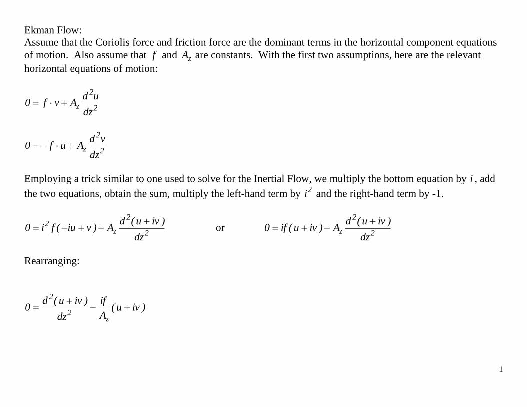
Ekman Flow:
Assume that the Coriolis force and friction force are the dominant terms in the horizontal component equations
of motion. Also assume that f and zA are constants. With the first two assumptions, here are the relevant
horizontal equations of motion:
2
2
zdz
udAvf0
2
2
zdz
vdAuf0
Employing a trick similar to one used to solve for the Inertial Flow, we multiply the bottom equation by i , add
the two equations, obtain the sum, multiply the left-hand term by 2i and the right-hand term by -1.
2
2
z2
dz
)ivu(dA)viu(fi0
or
2
2
zdz
)ivu(dA)ivu(if0
Rearranging:
)ivu(A
if
dz
)ivu(d0
z2
2
2
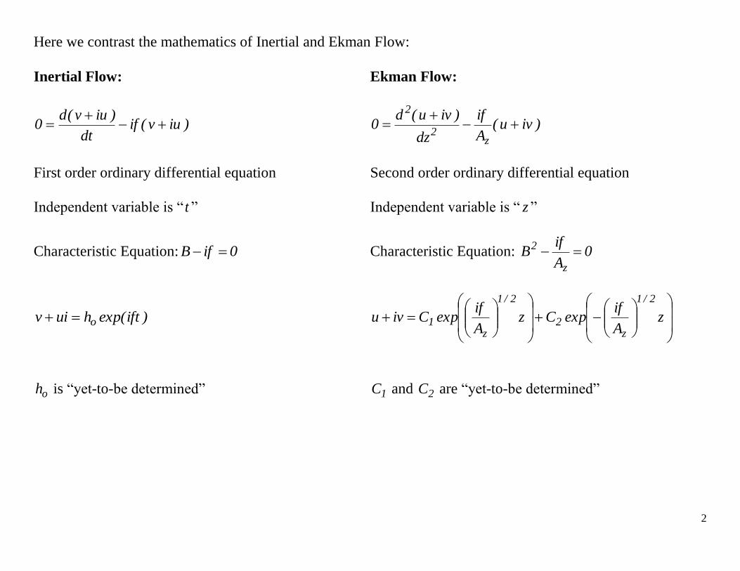
Here we contrast the mathematics of Inertial and Ekman Flow:
Inertial Flow: Ekman Flow:
)iuv(ifdt
)iuv(d0
)ivu(
A
if
dz
)ivu(d0
z2
2
First order ordinary differential equation Second order ordinary differential equation
Independent variable is “ t ” Independent variable is “ z ”
Characteristic Equation: 0ifB Characteristic Equation: 0A
ifB
z
2
)iftexp(huiv o
z
A
ifexpCz
A
ifexpCivu
2/1
z2
2/1
z1
oh is “yet-to-be determined” 1C and 2C are “yet-to-be determined”

3
There is an algebraic trick that we need to deal with:
2
1ii
(Easily derived: ?)1i)(1i( )
Hence, for the “ B” in the Ekman solution
2/1
z
2/1
z
2/1
z A2
f)1i(
A
f
2
1i
A
ifB
Here is result:
2/1
zA2
f)1i(B
(6)
4
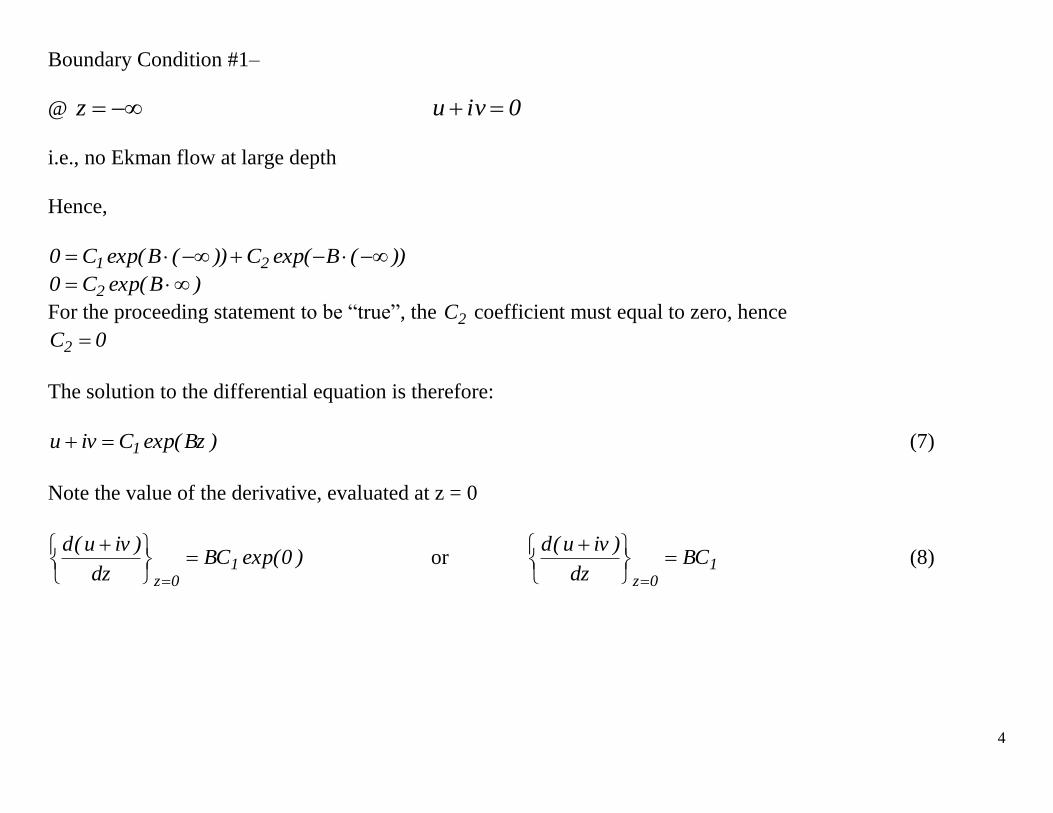
Boundary Condition #1–
@ z 0ivu
i.e., no Ekman flow at large depth
Hence,
))(Bexp(C))(Bexp(C0 21
)Bexp(C0 2
For the proceeding statement to be “true”, the 2C coefficient must equal to zero, hence
0C2
The solution to the differential equation is therefore:
)Bzexp(Civu 1 (7)
Note the value of the derivative, evaluated at z = 0
)0exp(BCdz
)ivu(d1
0z
or 10z
BCdz
)ivu(d
(8)
5
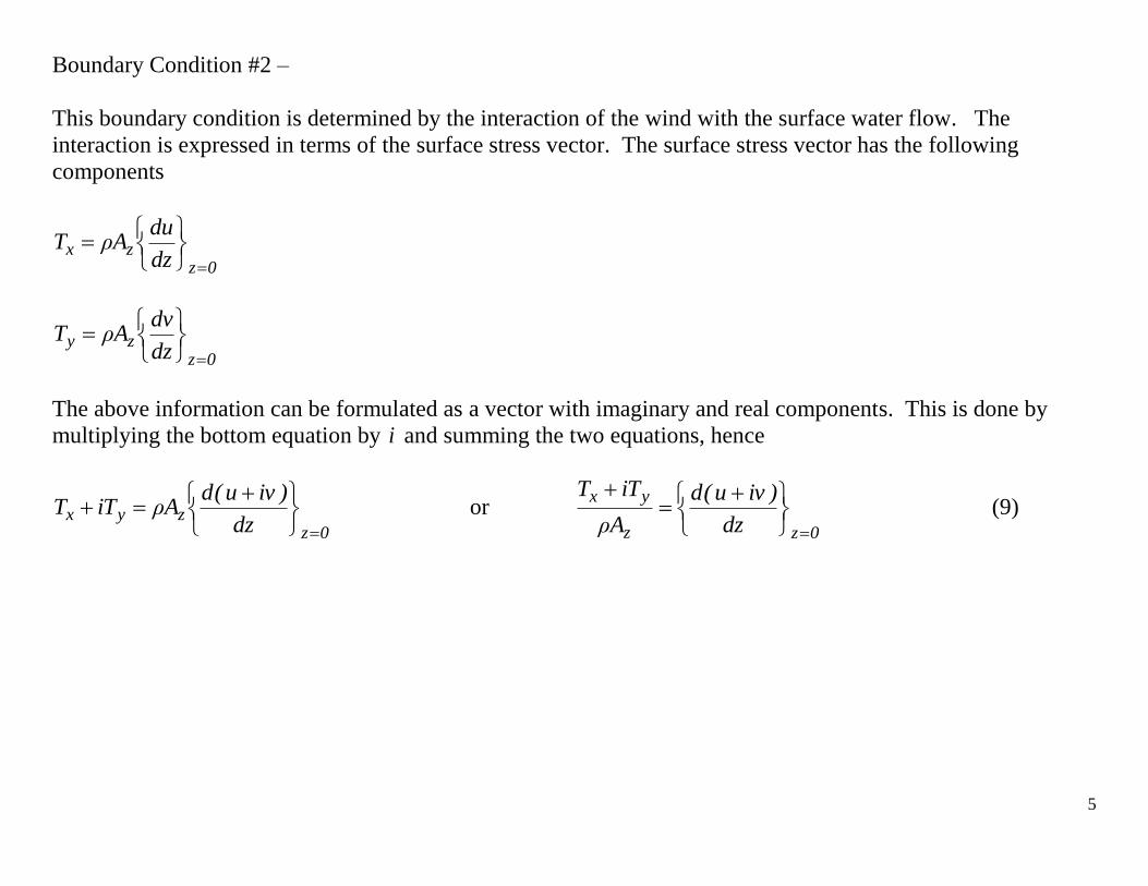
Boundary Condition #2 –
This boundary condition is determined by the interaction of the wind with the surface water flow. The
interaction is expressed in terms of the surface stress vector. The surface stress vector has the following
components
0zzx
dz
duAρT
0zzy
dz
dvAρT
The above information can be formulated as a vector with imaginary and real components. This is done by
multiplying the bottom equation by i and summing the two equations, hence
0zzyx
dz
)ivu(dAρiTT
or 0zz
yx
dz
)ivu(d
Aρ
iTT
(9)
6
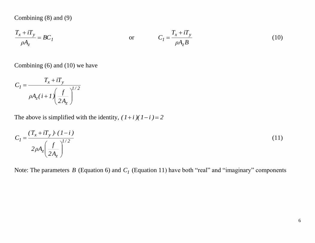
Combining (8) and (9)
1z
yxBC
Aρ
iTT
or
BAρ
iTTC
z
yx1
(10)
Combining (6) and (10) we have
2/1
zz
yx1
A2
f)1i(Aρ
iTTC
The above is simplified with the identity, 2)i1)(i1(
2/1
zz
yx1
A2
fAρ2
)i1()iTT(C
(11)
Note: The parameters B (Equation 6) and 1C (Equation 11) have both “real” and “imaginary” components
7
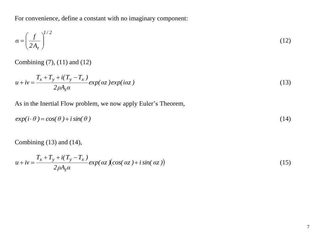
For convenience, define a constant with no imaginary component:
2/1
zA2
fα
(12)
Combining (7), (11) and (12)
)zαiexp()zαexp(αAρ2
)TT(iTTivu
z
xyyx (13)
As in the Inertial Flow problem, we now apply Euler’s Theorem,
)θsin(i)θcos()θiexp( (14)
Combining (13) and (14),
)zαsin(i)zαcos()zαexp(αAρ2
)TT(iTTivu
z
xyyx
(15)
8
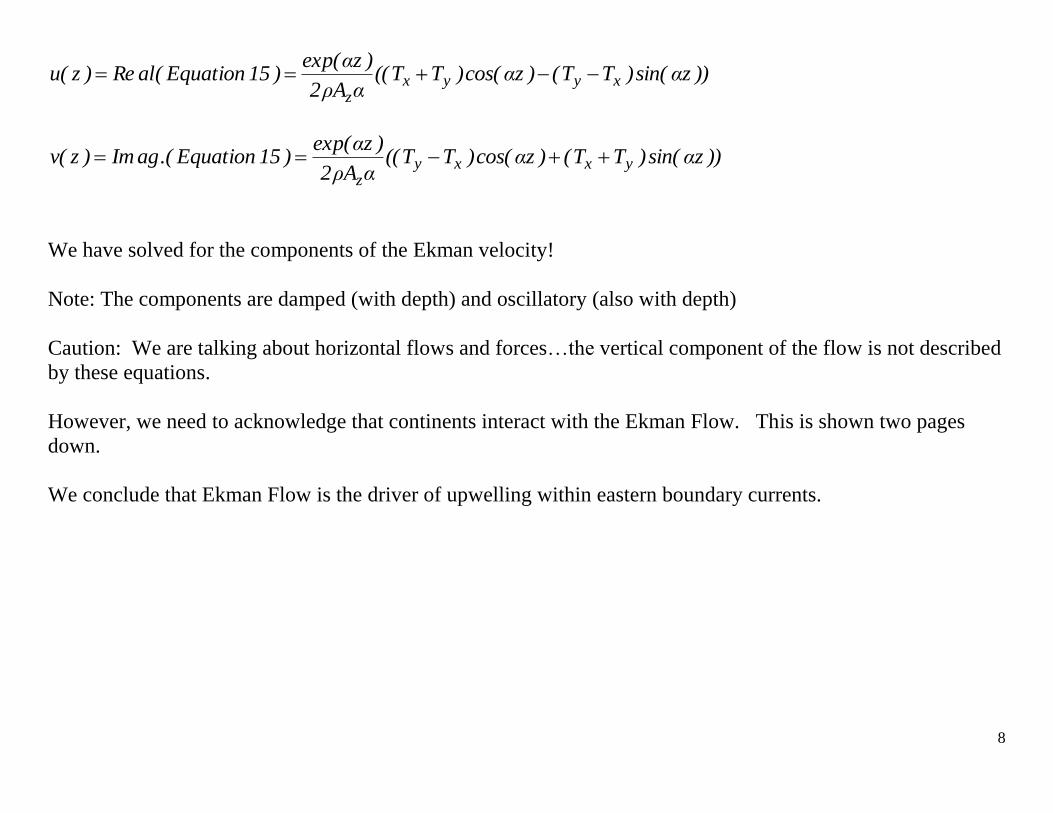
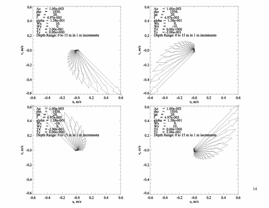
))zαsin()TT()zαcos()TT((αAρ2
)zαexp()15Equation(alRe)z(u xyyx
z
))zαsin()TT()zαcos()TT((αAρ2
)zαexp()15Equation.(agIm)z(v yxxy
z
We have solved for the components of the Ekman velocity!
Note: The components are damped (with depth) and oscillatory (also with depth)
Caution: We are talking about horizontal flows and forces…the vertical component of the flow is not described
by these equations.
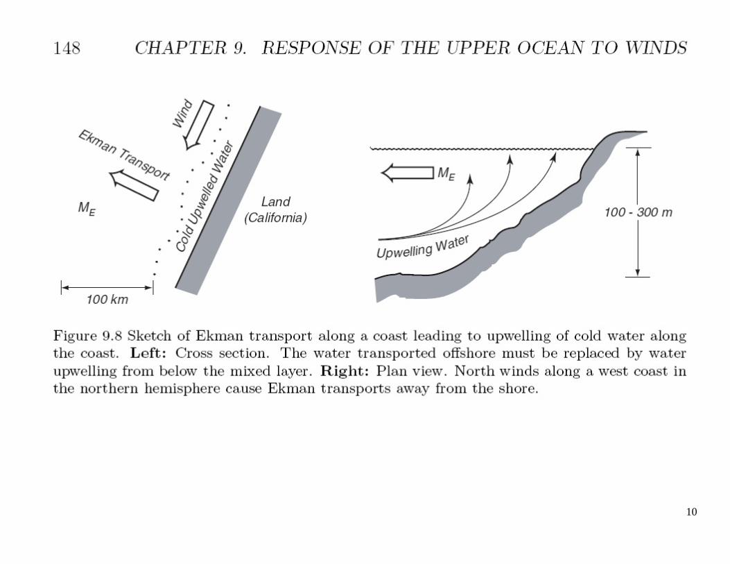
However, we need to acknowledge that continents interact with the Ekman Flow. This is shown two pages
down.
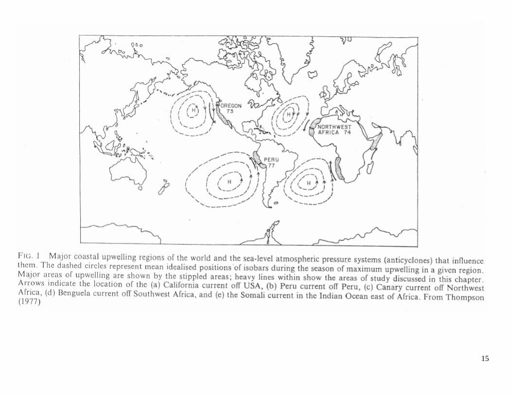
We conclude that Ekman Flow is the driver of upwelling within eastern boundary currents.
9
10
11
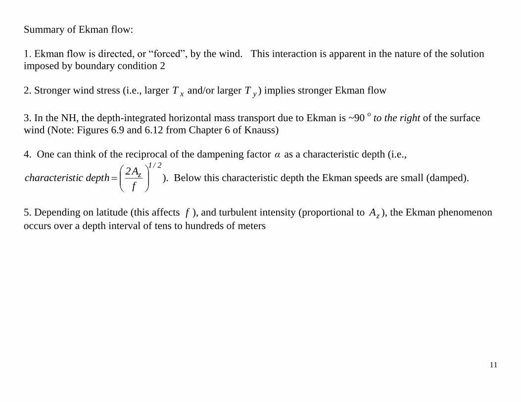
Summary of Ekman flow:
1. Ekman flow is directed, or “forced”, by the wind. This interaction is apparent in the nature of the solution
imposed by boundary condition 2
2. Stronger wind stress (i.e., larger xT and/or larger yT ) implies stronger Ekman flow
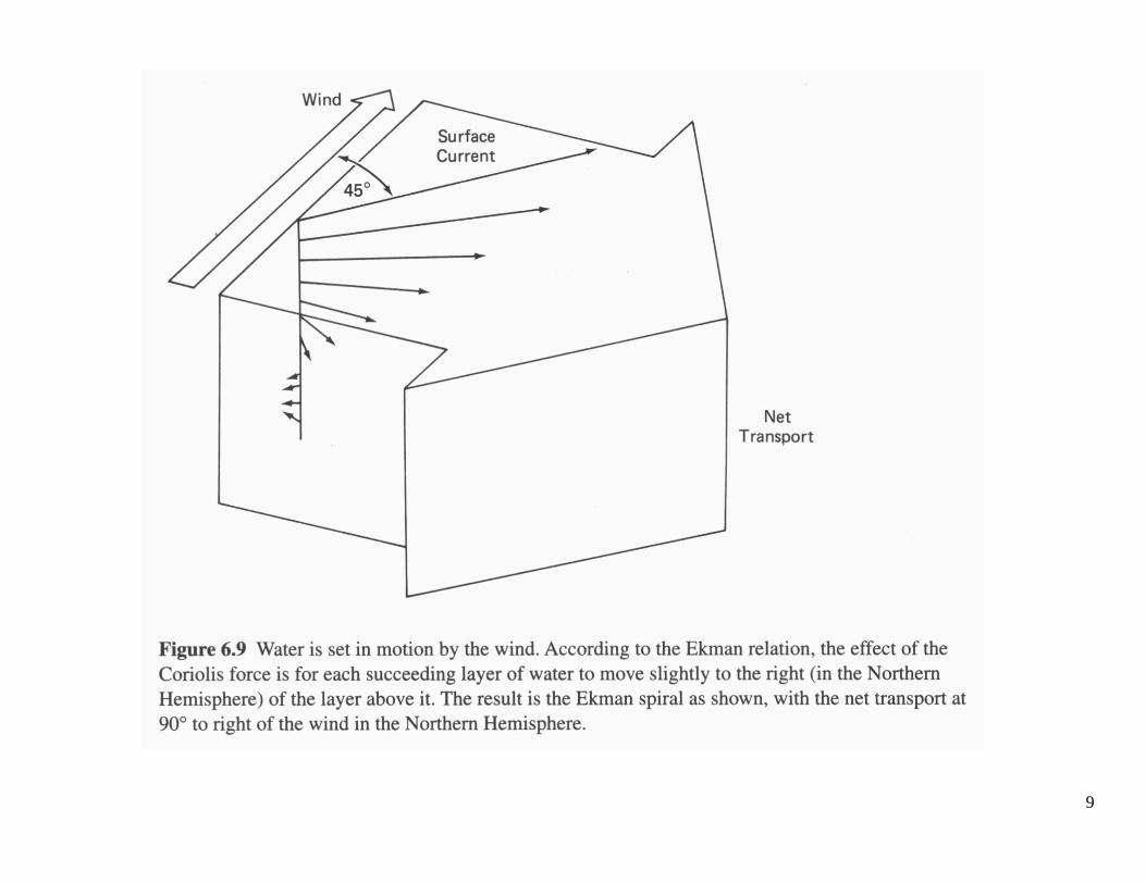
3. In the NH, the depth-integrated horizontal mass transport due to Ekman is ~90 o to the right of the surface
wind (Note: Figures 6.9 and 6.12 from Chapter 6 of Knauss)
4. One can think of the reciprocal of the dampening factor α as a characteristic depth (i.e., 2/1
z
f
A2depthsticcharacteri
). Below this characteristic depth the Ekman speeds are small (damped).
5. Depending on latitude (this affects f ), and turbulent intensity (proportional to zA ), the Ekman phenomenon
occurs over a depth interval of tens to hundreds of meters
12
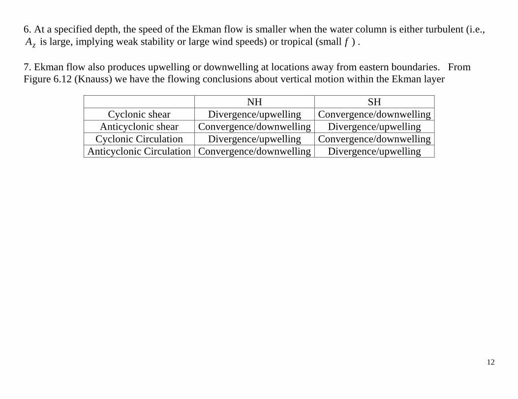
6. At a specified depth, the speed of the Ekman flow is smaller when the water column is either turbulent (i.e.,
zA is large, implying weak stability or large wind speeds) or tropical (small f ) .
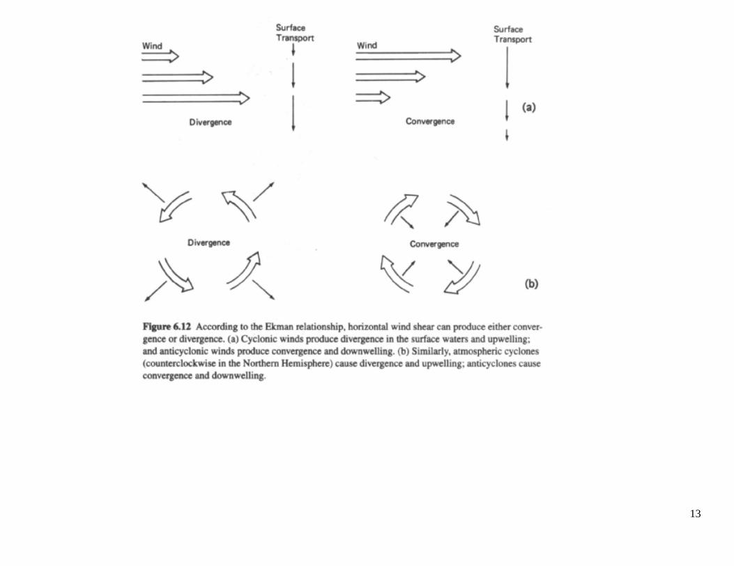
7. Ekman flow also produces upwelling or downwelling at locations away from eastern boundaries. From
Figure 6.12 (Knauss) we have the flowing conclusions about vertical motion within the Ekman layer
NH SH
Cyclonic shear Divergence/upwelling Convergence/downwelling
Anticyclonic shear Convergence/downwelling Divergence/upwelling
Cyclonic Circulation Divergence/upwelling Convergence/downwelling
Anticyclonic Circulation Convergence/downwelling Divergence/upwelling
13
14
15
Top Related