


Languages
Pages
Legal


Eigengene Network Analysis: MaleFemale Mouse Liver Comparison
R Tutorial Peter Langfelder and Steve Horvath
Correspondence: [email protected], [email protected]
This is a selfcontained R software tutorial that illustrates how to carry out an eigengene network analysis across two datasets. The two data sets correspond to gene expression measurements in the livers of male and female mice. This supplement describes the microarray data set. The R code allows to reproduce the Figures and tables reported in Langelder and Horvath (2007).Some familiarity with the R software is desirable but the document is fairly selfcontained. The data and biological implications are described in the following refence
• Langfelder P, Horvath S (2007) Eigengene networks for studying the relationships between coexpression modules. BMC Bioinformatics
To facilitate comparison with the original analysis, we use the microarray normalization procedures and gene selection procedures described in Ghazalpour et al (2006).
This tutorial and the data files can be found at the following webpage: http://www.genetics.ucla.edu/labs/horvath/CoexpressionNetwork/EigengeneNetworkMore material on weighted network analysis can be found herehttp://www.genetics.ucla.edu/labs/horvath/CoexpressionNetwork/
Microarray DataThe Agilent microarrays measured gene expression profiles in female mice of an F2mouse intercross described in Ghazalpour et al 2006. The gene expression data were obtained from liver tissues of male and female mice.The F2 mouse intercross data set (referred to as B × H cross) was obtained from liver tissues of female and male mice. The F2 intercross was based on the inbred strains C3H/HeJ and C57BL/6J (Ghazalpour et al. 2006; Wang et al. 2006).Body weight and related physiologic (“clinical”) traits were measured for the mice.B × H mice are ApoE null (ApoE −/−) and thus hyperlipidemic and were fed a highfat diet The B × H mice were sacrificed at 24 weeks.
BxH mouse data
For this analysis, we started with the 3421 genes (probesets) used in Ghazalpour et al 2006. The genes were the most connected genes among the 8000 most varying genes of the female liver dataset. We filtered out 6 genes that had zero variance in at least one of the four tissue datasets, leaving 3415 genes. For each of the datasets (corresponding to the 4 tissues), the Pearson correlation matrix of the genes was calculated and turned into adjacencies by raising the absolute value to power beta=6. From the adjacency matrices, we calculated the TOM similarities which were then used to calculate the consensus dissimilarity.The dissimilarity was used as input in averagelinkagehierarchical clustering. Branches of the resulting dendrogram were identified using the ``dynamic'' treecut algorithm used in Ghazalpour et al 2006. The maximum merging height for the cutting was set to 0.97, and minimum module size to 25. This procedure resulted in 12 initial consensus modules. To determine whether some of the initial consensus modules were too close, we calculated their eigengenes in each dataset, and formed their correlation matrices (one for each dataset). A ``minimum consensus similarity'' matrix was calculated as the minimum of the dataset eigengene correlation matrices; this matrix was turned into dissimilarity by subtracting it from one and used as input of averagelinkage hierarchical clustering again. In the resulting dendrogram of consensus modules, branches with merging height less than 0.25 were identified and modules on these branches were merged. Such branches correspond to modules whose eigengenes have a correlation of 0.75 or higher, which we judge to be close enough to be merged. This modulemerging procedure resulted in 11 final consensus modules that are described in the main text.
Animal husbandry and physiological trait measurements.C57BL/6J apoE null (B6.apoE−/−) mice were purchased from the Jackson Laboratory (Bar Harbor, Maine, United States) and C3H/HeJ apoE null (C3H.apoE−/−) mice were bred by backcrossing B6.apoE−/− to C3H/HeJ for ten generations with selection at each generation for the targeted ApoE−/− alleles on Chromosome 7. All mice were fed ad libidum and maintained on a 12h light/dark cycle. F2 mice were generated by crossing B6.apoE−/− with C3H.apoE−/− and subsequently intercrossing the F1 mice. F2 mice were fed Purina Chow (RalstonPurina Co., St. Louis, Missouri, United States)
Physiologic traitsThe original data Ghazalpour et al 2006 contain 26 traits, some of which are highly correlated. Here we consider 10 physiologic traits related to metabolic syndrome.To select independent traits, we clustered the traits with dissimilarity given by correlation
subtracted from one. Branches of the dendrogram correspond to groups of highly related traits; we chose a height cutoff of 0.35 (that is, correlation of 0.65) for the branch detection. For each branch, we selected a representative trait by taking the trait that is closest to the branch ``eigentrait'', that is the first principal component of the trait matrix (we would like to emphasize that the selected traits are actually measured traits and are not composite measurements). This procedure resulted in 20 traits. For brevity we only report significance for traits for which there is at least one module whose (eigengenetrait) correlation pvalue is 0.01 or less. This restriction leads to 6 potentially interesting traits which we used in the analysis of module significance used in the main text.
At the time of euthanasia, all mice were weighed and measured from the tip of the nose to the anus. Fat depots, plasma lipids (free fatty acids and triglycerides), plasma highdensity liporprotein (HDL) cholesterol and total cholesterol, and plasma insulin levels were measured as previously described. Very lowdensity lipoprotein (VLDL)/LDL cholesterol levels were calculated by subtracting HDL cholesterol from total cholesterol levels. Plasma glucose concentrations were measured using a glucose kit (#315–100; Sigma, St. Louis, Missouri, United States). Plasma leptin, adiponectin, and MCP1 levels were measured using mouse enzymelinked immunoabsorbent (ELISA) kits (#MOB00, #MRP300, and MJE00; R&D Systems, Minneapolis, Minnesota, United States).
Microarray analysis.RNA preparation and array hybridizations were performed at Rosetta Inpharmatics (Seattle, Washington, United States). The custom inkjet microarrays used in this study (Agilent Technologies [Palo Alto, California, United States], previously described [3,45]) contain 2,186 control probes and 23,574 noncontrol oligonucleotides extracted from mouse Unigene clusters and combined with RefSeq sequences and RIKEN fulllength clones. Mouse livers were homogenized and total RNA extracted using Trizol reagent (Invitrogen, Carlsbad, California, United States) according to manufacturer's protocol. Three g of total RNA was reverse transcribed and labeled with either Cy3 or Cy5 fluorochromes. Purified Cy3 or Cy5 complementary RNA was hybridized to at least two microarray slides with fluor reversal for 24 h in a hybridization chamber, washed, and scanned using a laser confocal scanner. Arrays were quantified on the basis of spot intensity relative to background, adjusted for experimental variation between arrays using average intensity over multiple channels, and fit to an error model to determine significance (type I error). Gene expression is reported as the ratio of the mean log10
intensity (mlratio) relative to the pool derived from 150 mice randomly selected from the F2 population.
Microarray data reduction.In order to minimize noise in the gene expression dataset, several datafiltering steps were taken. First, preliminary evidence showed major differences in gene expression levels between sexes among the F2 mice used, and therefore only female mice were used for network construction. The construction and comparison of the male network will be reported elsewhere. Only those mice with complete phenotype, genotype, and array data were used. This gave a final experimental sample of 135 female mice used for network construction. To reduce the computational burden and to possibly enhance the signal in our data, we used only the 8,000 mostvarying female liver genes in our preliminary network construction. For module detection, we limited our analysis to the 3,600 mostconnected genes because our module construction method and visualization tools cannot handle larger datasets at this point. By definition, module genes are highly connected with the genes of their module (i.e., module genes tend to have relatively high connectivity). Thus, for the purpose of module detection, restricting the analysis to the mostconnected genes should not lead to major information loss. Since the network nodes in our analysis correspond to genes as opposed to probesets, we eliminated multiple probes with similar expression patterns for the same gene. Specifically, the 3,600 genes were examined, and where appropriate, gene isoforms and genes containing duplicate probes were excluded by using only those with the highest expression among the redundant transcripts. This final filtering step yielded a count of 3,421 genes for the experimental network construction.
Weighted gene coexpression network construction.Constructing a weighted coexpression network is critical for identifying modules and for defining the intramodular connectivity. In coexpression networks, nodes correspond to genes, and connection strengths are determined by the pairwise correlations between expression profiles. In contrast to unweighted networks, weighted networks use soft thresholding of the Pearson correlation matrix for determining the connection strengths between two genes. Soft thresholding of the Pearson correlation preserves the continuous nature of the gene coexpression information, and leads to results that are highly robust with respect to the weighted network construction method (Zhang and Horvath 2005).The theory of the network construction algorithm is described in detail elsewhere Zhang and Horvath (2005). Briefly, a gene coexpression similarity measure (absolute value of the Pearson product moment correlation) was used to relate every pairwise gene–gene relationship. An adjacency matrix was then constructed using a “soft” power adjacency function aij = |cor(xi, xj)|^ where the absolute value of the Pearson correlation measures

gene is the coexpression similarity, and aij represents the resulting adjacency that measures the connection strengths. The network connectivity (kall) of the ith gene is the sum of the connection strengths with the other genes. This summation performed over all genes in a particular module is the intramodular connectivity (kin). The network satisfies scalefree topology if the connectivity distribution of the nodes follows an inverse power law, (frequency of connectivity p(k) follows an approximate inverse power law in k, i.e., p(k) ~ k^{−). We chose a power of = 6 based on the scalefree topology criterion. This criterion says that the power parameter, , is the lowest integer such that the resulting network satisfies approximate scalefree topology (linear model fitting index R2 of the regression line between log(p(k)) and log(k) is larger than 0.8). This criterion uses the fact that gene coexpression networks have been found to satisfy approximate scalefree topology. Since we are using a weighted network as opposed to an unweighted network, the biological findings are highly robust with respect to the choice of this power. Many coexpression networks satisfy the scalefree property only approximately.
Consensus module detection
Consensus module detection is similar to the individual dataset module detection in thatit uses hierarchical clustering of genes according to a measure of gene dissimilarity.We use a genegene ``consensus'' dissimilarity measure Dissim(i,j) as input of average linkage hierarchical clustering. We define modules as branches of the tree. To cutoff branches we use a fixed height cutoff. Modules must contains a minimum number n0 of genes.Module detection proceeds along the following steps. (1) perform a hierarchical clustering using the consensus dissimilarity measure;(2) cut the clustering tree at a fixed height cutoff;(3) each cut branch with at least n0 genes is considered a separate module;(4) all other genes are considered unassigned and are colored in ``grey''.The resulting modules will depend to some degree on the cut height and minimum size.
The analysis here is identical to the female fourtissue one described above; the only difference was that the maximum joining height for the consensus dendrogram was 0.995 to make our results easier to compare to Ghazalpour et al 2006. The minimum module size was dataset to 40.
Topological Overlap and Module DetectionA major goal of network analysis is to identify groups, or "modules", of densely interconnected genes. Such groups are often identified by searching for genes with similar
patterns of connection strengths to other genes, or high "topological overlap". It is important to recognize that correlation and topological overlap are very different ways of describing the relationship between a pair of genes: while correlation considers each pair of genes in isolation, topological overlap considers each pair of genes in relation to all other genes in the network. More specifically, genes are said to have high topological overlap if they are both strongly connected to the same group of genes in the network (i.e. they share the same "neighborhood"). Topological overlap thus serves as a crucial filter to exclude spurious or isolated connections during network construction (Yip and Horvath 2007). To calculate the topological overlap for a pair of genes, their connection strengths with all other genes in the network are compared. By calculating the topological overlap for all pairs of genes in the network, modules can be identified. The advantages and disadvantages of the topological overlap measure are reviewed in Yip and Horvath (2007) and Zhang and Horvath (2005).
Definition of the Eigengene Denote by X the expression data of a given module (rows are genes, columns are microarray samples).First, the gene expression data X are scaled so that each gene expression profile has mean 0 and variance 1. Next, the geneexpression data X are decomposed via singular value decomposition (X=UDVT) and the value of the first module eigengene, V1, represents the module eigengene. Specifically, V1 corresponds to the largest singular value.This definition is equivalent to defining the module eigengene as the first principal component of cor(t(X)), i.e. the correlation matrix of the gene expression data.
ReferencesThe microarray data and processing steps are described in
• Ghazalpour A, Doss S, Zhang B, Wang S, Plaisier C, Castellanos R, Brozell A, Schadt EE, Drake TA, Lusis AJ, Horvath S (2006) "Integrating Genetic and Network Analysis to Characterize Genes Related to Mouse Weight". PLoS Genetics. Volume 2 | Issue 8 | AUGUST 2006
The mouse cross is described in• Wang S, Yehya N, Schadt EE, Wang H, Drake TA, et al. (2006) Genetic and
genomic analysis of a fat mass trait with complex inheritance reveals marked sex specificity. PLoS Genet 2:e15
Weighted gene coexpression network analysis is described in

• Bin Zhang and Steve Horvath (2005) "A General Framework for Weighted Gene CoExpression Network Analysis", Statistical Applications in Genetics and Molecular Biology: Vol. 4: No. 1, Article 17.
Other references• Yip A, Horvath S (2007) Gene network interconnectedness and the generalized
topological overlap measure BMC Bioinformatics 2007, 8:22
# Absolutely no warranty on the code. Please contact Peter Langfelder and Steve Horvath #with suggestions.
# Downloading the R software# 1) Go to http://www.Rproject.org, download R and install it on your computer# After installing R, you need to install several additional R library packages: # For example to install Hmisc, open R, # go to menu "Packages\Install package(s) from CRAN", # then choose Hmisc. R will automatically install the package. # When asked "Delete downloaded files (y/N)? ", answer "y".# Do the same for some of the other libraries mentioned below. But note that # several libraries are already present in the software so there is no need to reinstall them.
# Download the zip file containing: # 1) R function file: "NetworkFunctions.txt", which contains several R functions # needed for Network Analysis. # 2) The data files and this tutorial
# Unzip all the files into the same directory.# The user should copy and paste the following script into the R session.# Text after "#" is a comment and is automatically ignored by R.
source("NetworkFunctionsMouse.R");
set.seed(1); #needed for .Random.seed to be defined
options(stringsAsFactors = FALSE);
# Read in the datasets
data = read.table("cnew_liver_bxh_f2female_8000mvgenes_p3600_UNIQUE_tommodules.xls", header=T, strip.white=T, comment.char="")
AllLiverColors = data$module;
data2 = read.csv("LiverMaleFromLiverFemale3600.csv", header=T, strip.white=T, comment.char="")data2_expr = data2[, c(9:(dim(data2)[2]))];
# Separate out auxiliary data
AuxData = data[,c(1:8,144:150)]names(AuxData) = colnames(data)[c(1:8,144:150)]ProbeNames = data[,1];SampleNames = colnames(data)[9:143];
# General settings and parameters
No.Sets = 2;Set.Labels = c("Female Liver", "Male Liver");ModuleMinSize = 40;
# Put the data into a standard "multi set" structure: vector of lists
ExprData = vector(mode = "list", length = No.Sets);ExprData[[1]] = list(data = data.frame(t(data[,c(1:8,144:150)])));ExprData[[2]] = list(data = data.frame(t(data2_expr)));
names(ExprData[[1]]$data) = ProbeNames;names(ExprData[[2]]$data) = data2[, 1];
ExprData = KeepCommonProbes(ExprData);
#Impute zeros into normalized ExprData for NAs
for (set in 1:No.Sets){ ExprData[[set]]$data = scale(ExprData[[set]]$data); ExprData[[set]]$data[is.na(ExprData[[set]]$data)] = 0;}
# Cleanup variables not needed anymore
rm(data, data2, data2_expr);collect_garbage();
# Read in the clinical trait data
trait_data = read.csv("ClinicalTraits.csv", header=T, strip.white=T, comment.char="");
Gender = trait_data$sex;
AllTraits = trait_data[, c(31, 16)];AllTraits = AllTraits[, c(2, 11:36) ];
# Put the traits into a structure resembling the structure of expression data# For each set only keep traits for the samples that also have expression data
Traits = vector(mode="list", length = No.Sets);for (set in 1:No.Sets){ SetSampleNames = data.frame(Names = row.names(ExprData[[set]]$data));
SetTraits = merge(SetSampleNames, AllTraits, by.y = "Mice", by.x = "Names", all = FALSE, sort = FALSE); Traits[[set]] = list(data = SetTraits[, 1]); row.names(Traits[[set]]$data) = SetTraits[,1 ];}
rm(AllTraits); rm(SetTraits); rm(SetSampleNames); rm(trait_data);
collect_garbage();
# More general settings and parameters
OutFileBase = "MouseFeMaleConsensus";OutDir = ""PlotDir = ""FuncAnnoDir = ""NetworkFile = "MouseFeMaleConsensusNetwork.RData";StandardCex = 1.4;
# Calculate standard weighted gene coexpression networks in all sets
Network = GetNetwork(ExprData = ExprData, DegreeCut = 0, BranchHeightCutoff = 0.985, ModuleMinSize = 80, verbose = 4);
#save(Network, file=NetworkFile);#load(file=NetworkFile);
LiverColors = AllLiverColors[Network$SelectedGenes];## Calculate and cluster consensus gene dissimilarity
ConsBranchHeightCut = 0.95; ConsModMinSize = ModuleMinSize;ConsModMinSize2 = 20;
Consensus = IntersectModules(Network = Network, ConsBranchHeightCut = ConsBranchHeightCut, ConsModMinSize = ConsModMinSize, verbose = 4)
# Detect modules in the dissimilarity for several cut heights
No.Genes = sum(Network$SelectedGenes);ConsCutoffs = seq(from = 0.945, to = 0.995, by = 0.01);No.Cutoffs = length(ConsCutoffs);ConsensusColor = array(dim = c(No.Genes, 2*No.Cutoffs));#ConsensusColor2 = array(dim = c(No.Genes, No.Cutoffs));for (cut in 1:No.Cutoffs){ ConsensusColor[ ,2*cut1] = labels2colors(cutreeDynamic(dendro = Consensus$ClustTree, deepSplit = FALSE, cutHeight = ConsCutoffs[cut], minClusterSize=ConsModMinSize, method ="tree")); ConsensusColor[ ,2*cut] = labels2colors(cutreeDynamic(dendro = Consensus$ClustTree,
deepSplit = FALSE, cutHeight = ConsCutoffs[cut], minClusterSize=ConsModMinSize2, method ="tree"));}
# Plot found module colors with the consensus dendrogram
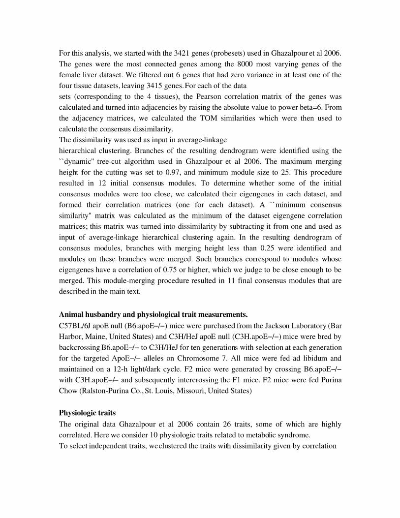
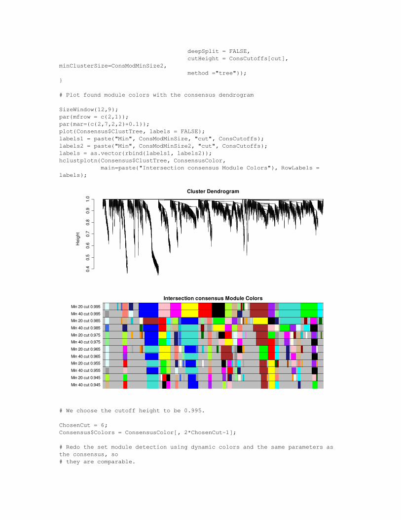
SizeWindow(12,9);par(mfrow = c(2,1));par(mar=(c(2,7,2,2)+0.1));plot(Consensus$ClustTree, labels = FALSE);labels1 = paste("Min", ConsModMinSize, "cut", ConsCutoffs);labels2 = paste("Min", ConsModMinSize2, "cut", ConsCutoffs);labels = as.vector(rbind(labels1, labels2));hclustplotn(Consensus$ClustTree, ConsensusColor, main=paste("Intersection consensus Module Colors"), RowLabels = labels);
0.4
0.5
0.6
0.7
0.8
0.9
1.0
Cluster Dendrogram
hclust (*, "average")as.dist(IntersectDissTOM)
Hei
ght
Intersection consensus Module Colors
Min 40 cut 0.945Min 20 cut 0.945Min 40 cut 0.955Min 20 cut 0.955Min 40 cut 0.965Min 20 cut 0.965Min 40 cut 0.975Min 20 cut 0.975Min 40 cut 0.985Min 20 cut 0.985Min 40 cut 0.995Min 20 cut 0.995
# We choose the cutoff height to be 0.995.
ChosenCut = 6;Consensus$Colors = ConsensusColor[, 2*ChosenCut1];
# Redo the set module detection using dynamic colors and the same parameters as the consensus, so# they are comparable.
ModuleMergeCut = 0.25;
MergedSetColors = Network$Colors;for (set in 1:No.Sets){ Network$Colors[, set] = labels2colors(cutreeDynamic(dendro = Network$ClusterTree[[set]]$data, deepSplit = FALSE, cutHeight= ConsCutoffs[ChosenCut], minClusterSize=ConsModMinSize, method = "tree")); MergedSetCols = MergeCloseModules(ExprData, Network, Network$Colors[, set], CutHeight = ModuleMergeCut, OnlySet = set, OrderedPCs = NULL, verbose = 4, print.level = 0); MergedSetColors[, set] = MergedSetCols$Colors; collect_garbage();}
# Calculate "raw" consensus MEs and plot them
PCs = NetworkModulePCs(ExprData, Network, UniversalModuleColors = Consensus$Colors, verbose=3)OrderedPCs = OrderPCs(PCs, GreyLast=TRUE, GreyName = "MEgrey");
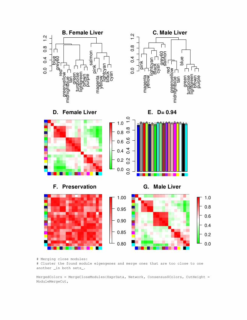
# Standard plot of differential eigengene network analysis
SizeWindow(7, 9);par(cex = StandardCex/1.4);PlotCorPCsAndDendros(OrderedPCs, Titles = Set.Labels, ColorLabels = TRUE, IncludeSign = TRUE, IncludeGrey = FALSE, plotCPMeasure = FALSE, plotMeans = T, CPzlim = c(0.8,1), plotErrors = TRUE, marHeatmap = c(1.6,2.7,1.6,6.0), marDendro = c(0.2,3,1.2,2), LetterSubPlots = TRUE, Letters = "BCDEFGHIJKLMNOPQRSTUV", PlotDiagAdj = TRUE);
blue
grey
60re
dgr
eeny
ello
wm
idni
ghtb
lue
tan
gree
ntu
rquo
ise
light
gree
nbr
own
purp
lesa
lmon
pink
mag
enta
yello
w light
cyan
blac
kcy
an0.0
0.4
0.8
1.2 B. Female Liver
pink
mag
enta
yello
w light
cyan
blac
kcy
angr
ey60
salm
onre
dgr
eeny
ello
wm
idni
ghtb
lue
tan
blue
gree
ntu
rquo
ise
light
gree
nbr
own
purp
le
0.0
0.4
0.8
1.2 C. Male Liver
D. Female Liver
0.0
0.2
0.4
0.6
0.8
1.0
E. D= 0.94
0.0
0.2
0.4
0.6
0.8
1.0
F. Preservation
0.80
0.85
0.90
0.95
1.00
G. Male Liver
0.0
0.2
0.4
0.6
0.8
1.0
# Merging close modules:# Cluster the found module eigengenes and merge ones that are too close to one another _in both sets_.
MergedColors = MergeCloseModules(ExprData, Network, Consensus$Colors, CutHeight = ModuleMergeCut,
OrderedPCs = OrderedPCs, IncludeGrey = FALSE, verbose = 4, print.level = 0);
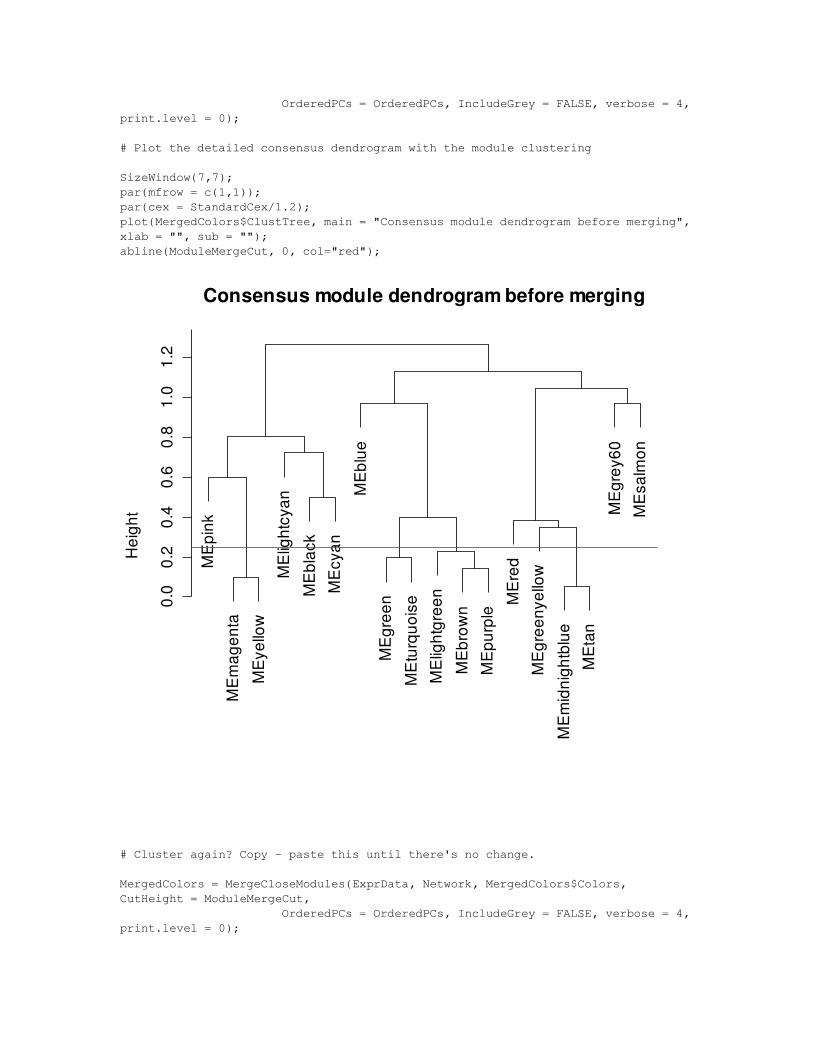
# Plot the detailed consensus dendrogram with the module clustering
SizeWindow(7,7);par(mfrow = c(1,1));par(cex = StandardCex/1.2);plot(MergedColors$ClustTree, main = "Consensus module dendrogram before merging", xlab = "", sub = "");abline(ModuleMergeCut, 0, col="red");
MEp
ink
MEm
agen
taM
Eyel
low
MEl
ight
cyan
MEb
lack
MEc
yan
MEb
lue
MEg
reen
MEt
urqu
oise
MEl
ight
gree
nM
Ebro
wnM
Epur
ple M
Ered
MEg
reen
yello
wM
Emid
nigh
tblu
eM
Etan
MEg
rey6
0M
Esal
mon
0.0
0.2
0.4
0.6
0.8
1.0
1.2
Consensus module dendrogram before merging
Heig
ht
# Cluster again? Copy paste this until there's no change.
MergedColors = MergeCloseModules(ExprData, Network, MergedColors$Colors, CutHeight = ModuleMergeCut, OrderedPCs = OrderedPCs, IncludeGrey = FALSE, verbose = 4, print.level = 0);
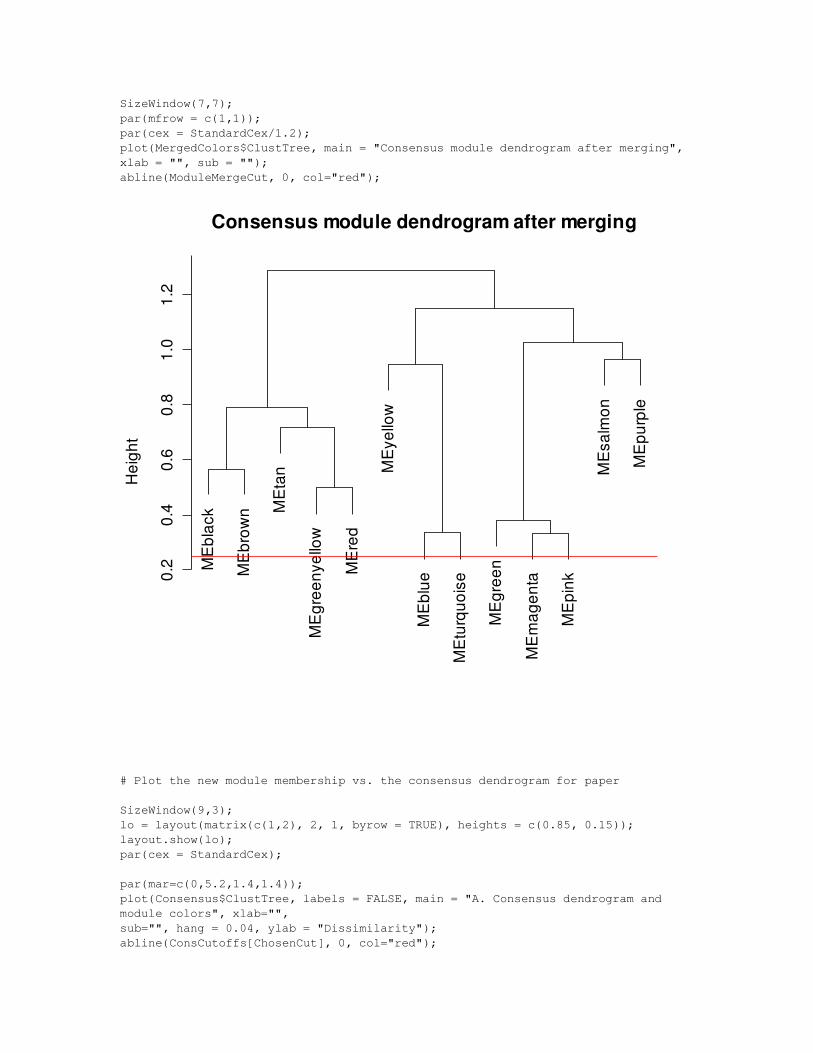
SizeWindow(7,7);par(mfrow = c(1,1));par(cex = StandardCex/1.2);plot(MergedColors$ClustTree, main = "Consensus module dendrogram after merging", xlab = "", sub = "");abline(ModuleMergeCut, 0, col="red");
MEb
lack
MEb
rown
MEt
an
MEg
reen
yello
w
MEr
ed
MEy
ello
w
MEb
lue
MEt
urqu
oise
MEg
reen
MEm
agen
ta
MEp
ink
MEs
alm
on
MEp
urpl
e
0.2
0.4
0.6
0.8
1.0
1.2
Consensus module dendrogram after merging
Heig
ht
# Plot the new module membership vs. the consensus dendrogram for paper
SizeWindow(9,3);lo = layout(matrix(c(1,2), 2, 1, byrow = TRUE), heights = c(0.85, 0.15));layout.show(lo);par(cex = StandardCex);
par(mar=c(0,5.2,1.4,1.4));plot(Consensus$ClustTree, labels = FALSE, main = "A. Consensus dendrogram and module colors", xlab="",sub="", hang = 0.04, ylab = "Dissimilarity");abline(ConsCutoffs[ChosenCut], 0, col="red");
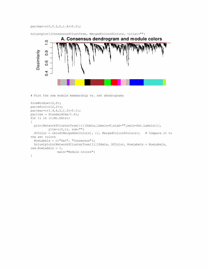
par(mar=c(0,5.2,0,1.4)+0.2);
hclustplot1(Consensus$ClustTree, MergedColors$Colors, title1="")
0.4
0.6
0.8
1.0 A. Consensus dendrogram and module colors
Diss
imila
rity
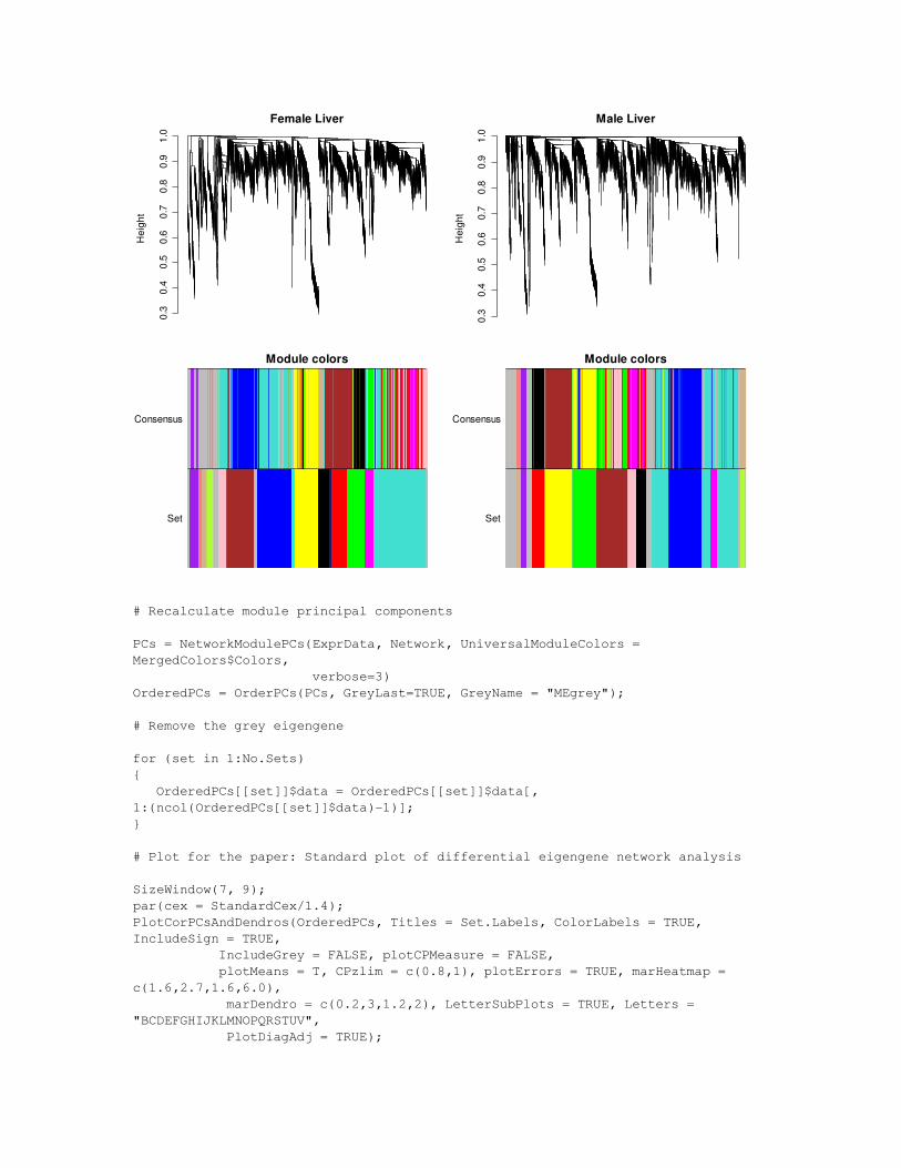
# Plot the new module membership vs. set dendrograms
SizeWindow(12,9);par(mfcol=c(2,2));par(mar=c(1.4,4,2,1.2)+0.1);par(cex = StandardCex/1.4);for (i in (1:No.Sets)){ plot(Network$ClusterTree[[i]]$data,labels=F,xlab="",main=Set.Labels[i], ylim=c(0,1), sub="") SCColor = cbind(MergedSetColors[, i], MergedColors$Colors); # Compare it to the set colors RowLabels = c("Set", "Consensus"); hclustplotn(Network$ClusterTree[[i]]$data, SCColor, RowLabels = RowLabels, cex.RowLabels = 1, main="Module colors")}
0.3
0.4
0.5
0.6
0.7
0.8
0.9
1.0
Female LiverH
eigh
t
Module colors
Set
Consensus
0.3
0.4
0.5
0.6
0.7
0.8
0.9
1.0
Male Liver
Hei
ght
Module colors
Set
Consensus
# Recalculate module principal components
PCs = NetworkModulePCs(ExprData, Network, UniversalModuleColors = MergedColors$Colors, verbose=3)OrderedPCs = OrderPCs(PCs, GreyLast=TRUE, GreyName = "MEgrey");
# Remove the grey eigengene
for (set in 1:No.Sets){ OrderedPCs[[set]]$data = OrderedPCs[[set]]$data[, 1:(ncol(OrderedPCs[[set]]$data)1)];}
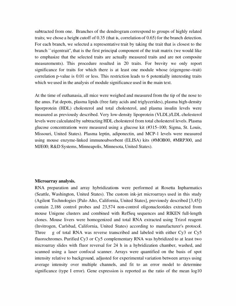
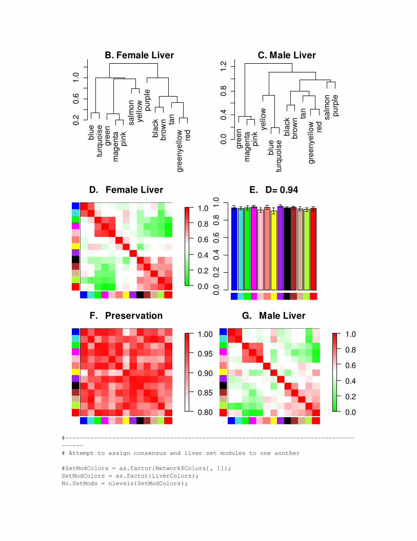
# Plot for the paper: Standard plot of differential eigengene network analysis
SizeWindow(7, 9);par(cex = StandardCex/1.4);PlotCorPCsAndDendros(OrderedPCs, Titles = Set.Labels, ColorLabels = TRUE, IncludeSign = TRUE, IncludeGrey = FALSE, plotCPMeasure = FALSE, plotMeans = T, CPzlim = c(0.8,1), plotErrors = TRUE, marHeatmap = c(1.6,2.7,1.6,6.0), marDendro = c(0.2,3,1.2,2), LetterSubPlots = TRUE, Letters = "BCDEFGHIJKLMNOPQRSTUV", PlotDiagAdj = TRUE);
blue
turq
uois
egr
een
mag
enta
pink
salm
onye
llow purp
lebl
ack
brow
n tan
gree
nyel
low red
0.2
0.6
1.0
B. Female Liver
gree
nm
agen
tapi
nkye
llow
blue
turq
uois
ebl
ack
brow
n tan
gree
nyel
low red
salm
onpu
rple
0.0
0.4
0.8
1.2
C. Male Liver
D. Female Liver
0.0
0.2
0.4
0.6
0.8
1.0
E. D= 0.94
0.0
0.2
0.4
0.6
0.8
1.0
F. Preservation
0.80
0.85
0.90
0.95
1.00
G. Male Liver
0.0
0.2
0.4
0.6
0.8
1.0
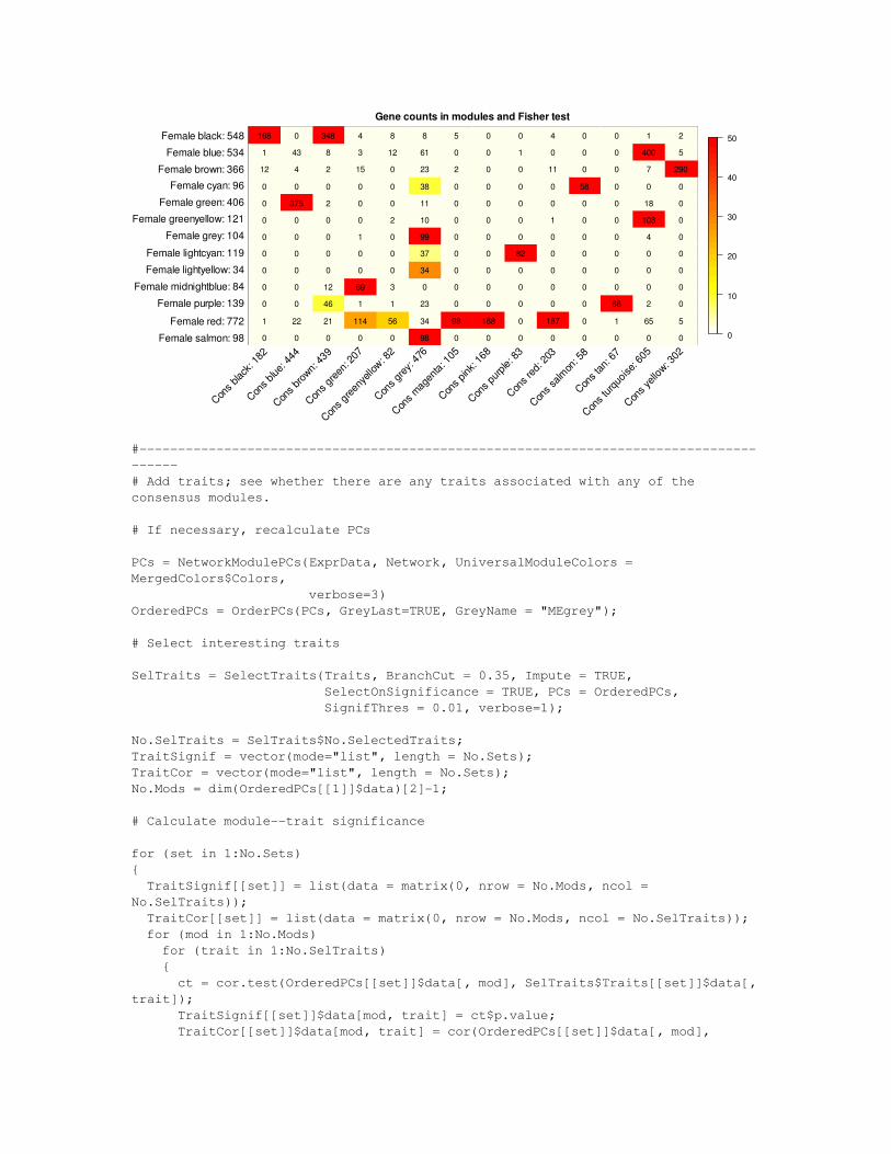
## Attempt to assign consensus and liver set modules to one another
#SetModColors = as.factor(Network$Colors[, 1]);SetModColors = as.factor(LiverColors);No.SetMods = nlevels(SetModColors);
ConsModColors = as.factor(MergedColors$Colors);No.ConsMods = nlevels(ConsModColors);
pTable = matrix(0, nrow = No.SetMods, ncol = No.ConsMods);CountTbl = matrix(0, nrow = No.SetMods, ncol = No.ConsMods);
for (smod in 1:No.SetMods) for (cmod in 1:No.ConsMods) { SetMembers = (SetModColors == levels(SetModColors)[smod]); ConsMembers = (ConsModColors == levels(ConsModColors)[cmod]); pTable[smod, cmod] = log10(fisher.test(SetMembers, ConsMembers, alternative = "greater")$p.value); CountTbl[smod, cmod] = sum(SetModColors == levels(SetModColors)[smod] & ConsModColors == levels(ConsModColors)[cmod]) }
pTable[is.infinite(pTable)] = 1.3*max(pTable[is.finite(pTable)]);pTable[pTable>50 ] = 50 ;
PercentageTbl = CountTbl;for (smod in 1:No.SetMods) PercentageTbl[smod, ] = as.integer(PercentageTbl[smod, ]/sum(PercentageTbl[smod, ]) * 100);
SetModTotals = as.vector(table(SetModColors));ConsModTotals = as.vector(table(ConsModColors));
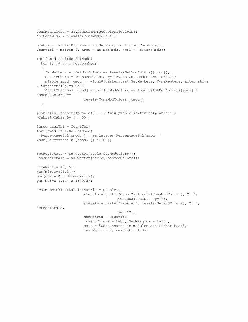
SizeWindow(10, 5);par(mfrow=c(1,1));par(cex = StandardCex/1.7);par(mar=c(8,12 ,2,1)+0.3);
HeatmapWithTextLabels(Matrix = pTable, xLabels = paste("Cons ", levels(ConsModColors), ": ", ConsModTotals, sep=""), yLabels = paste("Female ", levels(SetModColors), ": ", SetModTotals, sep=""), NumMatrix = CountTbl, InvertColors = TRUE, SetMargins = FALSE, main = "Gene counts in modules and Fisher test", cex.Num = 0.8, cex.lab = 1.0);
Gene counts in modules and Fisher test
0
10
20
30
40
50
Cons b
lack:
182
Cons b
lue: 4
44
Cons b
rown:
439
Cons g
reen:
207
Cons g
reeny
ellow: 8
2
Cons g
rey: 4
76
Cons m
agen
ta: 10
5
Cons p
ink: 1
68
Cons p
urple:
83
Cons r
ed: 2
03
Cons s
almon
: 58
Cons t
an: 6
7
Cons t
urquo
ise: 6
05
Cons y
ellow: 3
02Female salmon: 98
Female red: 772Female purple: 139
Female midnightblue: 84Female lightyellow: 34Female lightcyan: 119
Female grey: 104Female greenyellow: 121
Female green: 406Female cyan: 96
Female brown: 366Female blue: 534
Female black: 548 168 0 348 4 8 8 5 0 0 4 0 0 1 2
1 43 8 3 12 61 0 0 1 0 0 0 400 5
12 4 2 15 0 23 2 0 0 11 0 0 7 290
0 0 0 0 0 38 0 0 0 0 58 0 0 0
0 375 2 0 0 11 0 0 0 0 0 0 18 0
0 0 0 0 2 10 0 0 0 1 0 0 108 0
0 0 0 1 0 99 0 0 0 0 0 0 4 0
0 0 0 0 0 37 0 0 82 0 0 0 0 0
0 0 0 0 0 34 0 0 0 0 0 0 0 0
0 0 12 69 3 0 0 0 0 0 0 0 0 0
0 0 46 1 1 23 0 0 0 0 0 66 2 0
1 22 21 114 56 34 98 168 0 187 0 1 65 5
0 0 0 0 0 98 0 0 0 0 0 0 0 0
## Add traits; see whether there are any traits associated with any of the consensus modules.
# If necessary, recalculate PCs
PCs = NetworkModulePCs(ExprData, Network, UniversalModuleColors = MergedColors$Colors, verbose=3)OrderedPCs = OrderPCs(PCs, GreyLast=TRUE, GreyName = "MEgrey");
# Select interesting traits
SelTraits = SelectTraits(Traits, BranchCut = 0.35, Impute = TRUE, SelectOnSignificance = TRUE, PCs = OrderedPCs, SignifThres = 0.01, verbose=1);
No.SelTraits = SelTraits$No.SelectedTraits;TraitSignif = vector(mode="list", length = No.Sets);TraitCor = vector(mode="list", length = No.Sets);No.Mods = dim(OrderedPCs[[1]]$data)[2]1;
# Calculate moduletrait significance
for (set in 1:No.Sets){ TraitSignif[[set]] = list(data = matrix(0, nrow = No.Mods, ncol = No.SelTraits)); TraitCor[[set]] = list(data = matrix(0, nrow = No.Mods, ncol = No.SelTraits)); for (mod in 1:No.Mods) for (trait in 1:No.SelTraits) { ct = cor.test(OrderedPCs[[set]]$data[, mod], SelTraits$Traits[[set]]$data[, trait]); TraitSignif[[set]]$data[mod, trait] = ct$p.value; TraitCor[[set]]$data[mod, trait] = cor(OrderedPCs[[set]]$data[, mod],
SelTraits$Traits[[set]]$data[, trait]); }}
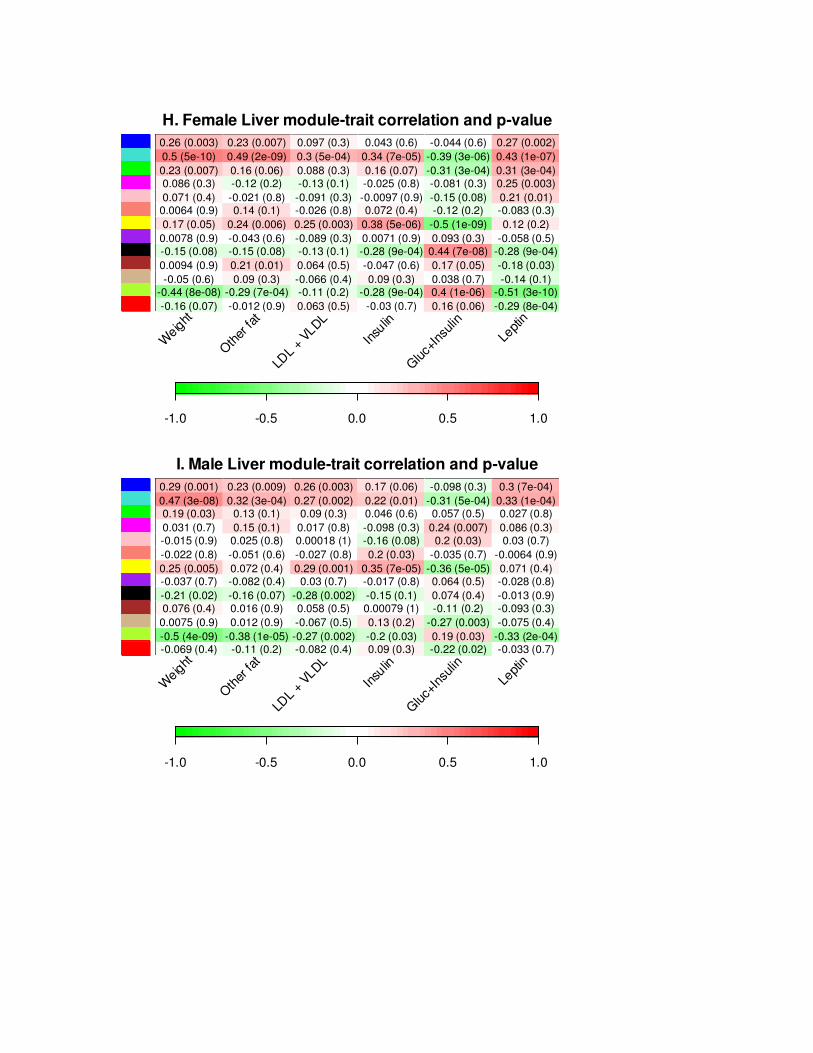
# Plot the significance heatmap
minp = 1; maxp = 0;for (set in 1:No.Sets){ minp = min(minp, TraitSignif[[set]]$data); maxp = max(maxp, TraitSignif[[set]]$data);}# To make the plots mangeable: leave out the "BMD femurs only" trait
#TraitLabels = c("Weight", "Other fat", "LDL + VLDL", "Insulin", # "Gluc+Insulin", "Leptin", "BMD femurs only");TraitLabels = c("Weight", "Other fat", "LDL + VLDL", "Insulin", "Gluc+Insulin", "Leptin");
for (set in 1:No.Sets){ TraitSignif[[set]]$data = TraitSignif[[set]]$data[, ncol(TraitSignif[[set]]$data)]; TraitCor[[set]]$data = TraitCor[[set]]$data[, ncol(TraitCor[[set]]$data)];}
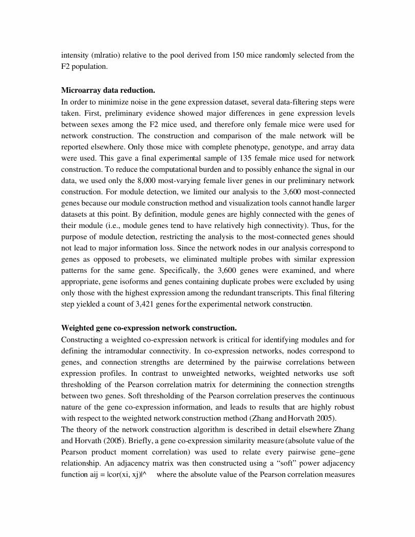
# Make the plot for the paper
SizeWindow(4.6,7.0);par(mfrow = c(2,1));par(mar = c(8, 2,2.2,1));
Letters = "HIJKL";letterInd = 1;for (set in 1:No.Sets){ par(cex = StandardCex/1.7); letter = paste(substring(Letters, set, set), ".", sep = ""); NumMatrix = paste(signif(TraitCor[[set]]$data,2)," (", signif(TraitSignif[[set]]$data,1), ")", sep=""); dim(NumMatrix) = dim(TraitCor[[set]]$data); # m = log10(TraitSignif[[set]]$data); HeatmapWithTextLabels(Matrix = TraitCor[[set]]$data, yLabels = names(OrderedPCs[[1]]$data)[c(1:No.Mods)], xLabels = TraitLabels, NumMatrix = NumMatrix, cex.Num = StandardCex/2.0, cex.lab = StandardCex/1.7, InvertColors = FALSE, SetMargins = FALSE, xColorLabels = FALSE, yColorLabels = TRUE, main = paste(letter, Set.Labels[set], "moduletrait correlation and pvalue"), color = GreenWhiteRed(50), #zlim = c(log10(maxp), log10(minp))); zlim = c(1, 1), horizontal = TRUE, legend.mar = 5);}
H. Female Liver moduletrait correlation and pvalue
1.0 0.5 0.0 0.5 1.0
Weight
Other fa
t
LDL +
VLDLIns
ulin
Gluc+In
sulin
Leptin
0.26 (0.003) 0.23 (0.007) 0.097 (0.3) 0.043 (0.6) 0.044 (0.6) 0.27 (0.002)0.5 (5e10) 0.49 (2e09) 0.3 (5e04) 0.34 (7e05) 0.39 (3e06) 0.43 (1e07)0.23 (0.007) 0.16 (0.06) 0.088 (0.3) 0.16 (0.07) 0.31 (3e04) 0.31 (3e04)0.086 (0.3) 0.12 (0.2) 0.13 (0.1) 0.025 (0.8) 0.081 (0.3) 0.25 (0.003)0.071 (0.4) 0.021 (0.8) 0.091 (0.3) 0.0097 (0.9) 0.15 (0.08) 0.21 (0.01)
0.0064 (0.9) 0.14 (0.1) 0.026 (0.8) 0.072 (0.4) 0.12 (0.2) 0.083 (0.3)0.17 (0.05) 0.24 (0.006) 0.25 (0.003) 0.38 (5e06) 0.5 (1e09) 0.12 (0.2)
0.0078 (0.9) 0.043 (0.6) 0.089 (0.3) 0.0071 (0.9) 0.093 (0.3) 0.058 (0.5)0.15 (0.08) 0.15 (0.08) 0.13 (0.1) 0.28 (9e04) 0.44 (7e08) 0.28 (9e04)0.0094 (0.9) 0.21 (0.01) 0.064 (0.5) 0.047 (0.6) 0.17 (0.05) 0.18 (0.03)0.05 (0.6) 0.09 (0.3) 0.066 (0.4) 0.09 (0.3) 0.038 (0.7) 0.14 (0.1)
0.44 (8e08) 0.29 (7e04) 0.11 (0.2) 0.28 (9e04) 0.4 (1e06) 0.51 (3e10)0.16 (0.07) 0.012 (0.9) 0.063 (0.5) 0.03 (0.7) 0.16 (0.06) 0.29 (8e04)
I. Male Liver moduletrait correlation and pvalue
1.0 0.5 0.0 0.5 1.0
Weight
Other fa
t
LDL +
VLDLIns
ulin
Gluc+In
sulin
Leptin
0.29 (0.001) 0.23 (0.009) 0.26 (0.003) 0.17 (0.06) 0.098 (0.3) 0.3 (7e04)0.47 (3e08) 0.32 (3e04) 0.27 (0.002) 0.22 (0.01) 0.31 (5e04) 0.33 (1e04)0.19 (0.03) 0.13 (0.1) 0.09 (0.3) 0.046 (0.6) 0.057 (0.5) 0.027 (0.8)0.031 (0.7) 0.15 (0.1) 0.017 (0.8) 0.098 (0.3) 0.24 (0.007) 0.086 (0.3)0.015 (0.9) 0.025 (0.8) 0.00018 (1) 0.16 (0.08) 0.2 (0.03) 0.03 (0.7)0.022 (0.8) 0.051 (0.6) 0.027 (0.8) 0.2 (0.03) 0.035 (0.7) 0.0064 (0.9)0.25 (0.005) 0.072 (0.4) 0.29 (0.001) 0.35 (7e05) 0.36 (5e05) 0.071 (0.4)0.037 (0.7) 0.082 (0.4) 0.03 (0.7) 0.017 (0.8) 0.064 (0.5) 0.028 (0.8)0.21 (0.02) 0.16 (0.07) 0.28 (0.002) 0.15 (0.1) 0.074 (0.4) 0.013 (0.9)0.076 (0.4) 0.016 (0.9) 0.058 (0.5) 0.00079 (1) 0.11 (0.2) 0.093 (0.3)
0.0075 (0.9) 0.012 (0.9) 0.067 (0.5) 0.13 (0.2) 0.27 (0.003) 0.075 (0.4)0.5 (4e09) 0.38 (1e05) 0.27 (0.002) 0.2 (0.03) 0.19 (0.03) 0.33 (2e04)0.069 (0.4) 0.11 (0.2) 0.082 (0.4) 0.09 (0.3) 0.22 (0.02) 0.033 (0.7)
Top Related