


Languages
Pages
Legal


Electronic copy available at: http://ssrn.com/abstract=2252174
Effortless Perfection:Do Chinese Cities Manipulate ”Blue Skies?”∗
Dalia Ghanem† Junjie Zhang ‡
University of California, San Diego
April 16, 2013
Abstract
It is alleged that some Chinese cities manipulate their air pollution data to comply withthe air quality standards set by the central government of China. This paper tests this hy-pothesis by using a unique data set. First, we employ a discontinuity test to detect the citiesthat reported dubious pollution data around the cutoff for ”blue-sky days.” Then, we proposea panel matching approach to identify the conditions under which irregularities may occur.Over the period 2001-2010, 55% of cities reported dubious PM10 pollution levels that led to adiscontinuity at the cutoff. Suspicious data reporting tends to occur on days when the potentialmanipulation is least detectable. Our findings indicate that the official daily air pollution dataare not well behaved, which provides suggestive evidence of manipulation.
Keywords: air pollution, manipulation, discontinuity test, panel matching.
JEL Classification Numbers: Q53 C23 C14.
∗The authors thank the UC Center for Energy and Environmental Economics (UCE3) for partial financial support.We thank Roger Bohn, Richard Carson, Graham Elliott, Josh Graff-Zivin, Mark Jacobsen, David Meyer, Steven Oliver,and Logan Smith for their helpful suggestions. We also benefited from the comments and suggestions from the seminardiscussants and participants at UCSD and AERE meetings. Of course, all remaining errors are ours.†Department of Economics, University of California, San Diego. [email protected].‡Corresponding Author. School of International Relations & Pacific Studies, University of California, San Diego.
9500 Gilman Drive #0519, La Jolla, CA 92093-0519. Tel: (858) 822-5733. Fax: (858) 534-3939. [email protected].

Electronic copy available at: http://ssrn.com/abstract=2252174
1 Introduction
Air quality of major Chinese cities is among the worst in the world, a consequence of three decades
of double-digit economic growth with lax environmental regulation (Zhang and Crooks, 2012).
The central government of China started to address the issue of environmental regulation. Over
a decade ago, major Chinese cities were required to report their daily air pollution index (API)
and to make it available to the public. To incentivize air pollution abatement, performance eval-
uations of local officials included the number of ”blue-sky days,” which are days with API below
100.1 These measures introduced both bottom-up and top-down pressures on the local govern-
ments to meet the target number of blue-sky days. In the absence of independent verification
mechanisms, some cities are allegedly under-reporting their air pollution levels. The presence of
a particular threshold for blue-sky days seems to be associated with dubious behavior of the API
scores around the cut-off, which is illustrated in Figure 1. We call this phenomenon ”effortless per-
fection.” Specifically, the API distributions of three municipalities, including Beijing, Tianjin and
Chongqing, amass right below the cut-off. The irregularities have raised suspicion of systematic
manipulation of air pollution data in China.
At the heart of this paper is a question about self-reported data that are used in performance
evaluations of the reporting agencies. In such settings, there is good reason to suspect that the
agencies manipulate the data to improve their performance evaluations, especially if such ma-
nipulation can go undetected. The relevance of this paper is hence not restricted to air pollution
reporting. Using the unique data set that we have, our main goal is to understand if and how ma-
nipulation occurs in this setup. The importance of such a question goes beyond detecting cheaters.
It can help us understand how manipulation can undermine the use of such self-reported data in
economic studies.
Data manipulation is a concern for both policy makers and researchers. For policy makers,
data manipulation defeats the purpose of policies that incentivize pollution abatement and other
policy objectives. It might be effortless for a city to beautify its environmental record by just tweak-
ing the numbers. However, society must then bear the costly consequence of misleading pollution
data. First, misinformed urban residents cannot efficiently mitigate pollution-related health effects
1A blue-sky day is associated with low or moderate health concerns. See Table 3 for categories of API and healthconcerns.
1

by changing their behavior, for example wearing masks or canceling outdoor activities. Second,
promotion of officials whose cities have become involved in manipulation jeopardizes the pub-
lic interest because their integrity is in question. In addition, environmental compliance through
manipulation undermines the government’s credibility.
Manipulation introduces measurement error into the data that may be used as regressors to
study the effect of pollution on health and other outcomes. Such measurement error will bias
studies that evaluate the impact of air pollution using such data on various outcomes.2 The biased
marginal effects of pollution might lead to incorrect policy recommendations. If the measurement
error in the air pollution data violates the classical measurement-error assumptions, then standard
econometric methods may not rectify the bias due to the measurement error in this data.
Our paper aims to identify irregularities in the air pollution data in order to provide insight
on the nature of manipulation and the circumstances under which it occurs. We define manipu-
lation as the behavior of not reporting the true pollution level, such as data falsification or hiding
bad pollution data. It does not include strategic behavior such as temporary driving bans, closing
factories, or requiring different fuels.3 Although these command-and-control policies are ineffi-
cient, they can indeed reduce pollution in the short run so we cannot call them manipulation. The
best way to detect manipulation is to use alternative sources of data to validate the official data.
However, independent direct measures are not available for all the relevant pollutants, cities, and
periods.4 Therefore, this paper uses econometric methods to uncover suggestive evidence of ma-
nipulation from the self-reported data.
We pose two research questions. First, we investigate whether a city reports dubious pollution
data around the cutoff for blue-sky days.5 To answer this question, our empirical strategy is bor-
rowed from the McCrary (2008) test, which is used to detect manipulation of a running variable
2A large body of literature in environmental and health economics studies the impact of air pollution on productivity(Koop and Tole, 2004), property values (Chay and Greenstone, 2005), and health (Graff Zivin and Neidell, 2012). Thereliability of the estimated marginal effects hinges on valid pollution data.
3These policies were used during major events such as 2008 Olympic Games in Beijing and Expo 2010 in Shanghai.They are also used when local governments are desperate to meet their environmental targets at the end of a particularyear.
4A notable independent measure is the U.S Embassy Beijing Air Quality Monitor. It has reported PM2.5 particulatespollution since 2008. However, PM2.5 was not regulated during 2001-2010. Some research institutions collected airquality data independently but the data are not widely available.
5Moral hazard arises where there is a cut-off in the performance evaluation and the information is asymmetric.Manipulation around the cut-off is not a unique phenomenon in economics. For example, lenders treat mortgageborrowers with credit scores just above certain thresholds differently from those with slightly lower scores. Borrowersmay take advantage of this rule of screening by manipulating their FICO scores (Keys et al., 2010).
2

in regression discontinuity design. The intuition here is that if the pollutant concentration on a
particular day misses the cutoff for blue-sky day by a small amount, then there is an incentive
for the city to under-report the pollutant concentration and score a blue-sky day. If such behavior
occurs often, the distribution of the pollutant concentration exhibits a discontinuity at the cutoff
for a blue-sky day. In the absence of manipulation, the distribution of air pollutant concentrations
is expected to be continuous because polluters and regulators do not have complete control over
the realized pollutant concentration (Brannlund and Lofgren, 1996). Thus, detection of this type
of manipulation boils down to a test of discontinuity around the cutoff for blue-sky days in the
distribution of pollutant concentrations. Irregularity around the cut-off is a red flag of potential
manipulation.6
Second, we study the patterns of manipulation by proposing a panel matching approach. The
ideal experiment to examine such patterns is to observe twin cities that are expected to have iden-
tical distributions of air quality, and hence of the API. The panel matching approach constructs
pairs of cities that have the same geographic and provincial characteristics. Since true air quality
is unobservable, we use visibility as a proxy together with other weather variables (Sloane and
White, 1986). The key assumption that allows us to identify manipulation is that for a constructed
city pair, we expect that the two cities have the same distribution of API conditional on visibil-
ity and other weather variables. This approach does not pin down the manipulator.7 Instead, it
identifies the conditions under which manipulation is most likely to occur.
This paper is not the first attempt to investigate dubious air pollution data in China. Andrews
(2008a,b) first questioned the credibility of official data in Beijing and brought this issue to pub-
lic attention. The author presented the evidence that the API has massive bunching below the
cut-off in addition to other gimmicks to polish air quality reports. Chen et al. (2012) provide a for-
mal econometric analysis on the accuracy of the air pollution data. They confirmed the anomaly
around the cut-off based on the official data from 37 large cities during 2000-2009. We improve on
this literature in three aspects.
First, we use a more comprehensive data set. In particular, we obtained the confidential daily
6As noted above, command-and-control policies can also be used to ensure that the target number of blue-sky daysis met. Such behavior can also lead to a bunching below the cutoff for blue-sky days.
7Inspection of the empirical CDFs can suggest which city is the manipulator, but the formal tests we perform do notanswer this question.
3

air pollution data from the China National Environmental Monitoring Center (CNEMC). The data
include non-disclosed variables underlying the calculation of the API. Our data set covers 113
cities during 2001-2010, which includes all cities that are required to disclose daily air pollution
information. The detailed data have never been used in previous studies.
Second, our data set allows us to apply the discontinuity test to pollutant concentrations di-
rectly instead of the API. The distribution of pollutant concentrations satisfies the continuity as-
sumption of the McCrary (2008) test, hereinafter the McCrary test, whereas that of the API does
not. The API is a nonlinear transformation of pollutant concentrations. Its distribution is not con-
tinuous, which violates the assumption required for the McCrary test. Applying the McCrary test
to the API scores directly may lead to biased results.
Third, our panel matching method is novel. The nonparametric specification is superior to a
linear model because the former does not assume that manipulation and control variables such
as visibility and weather conditions are separable, which allows for more realistic forms of ma-
nipulation which differ based on weather conditions. Furthermore, linear fixed effects models are
known to be inconsistent when they are misspecified as shown in Chernozhukov et al. (2010) and
Gibbons, Serrato, and Urbancic (2011). Since we do not expect the true relationship between API
and other variables to be linear or to follow a particular functional form assumption, the nonpara-
metric approach is preferable.
Our primary finding is that 55% of cities report dubious particulate matter (PM10) pollution
data. In comparison, the data for sulfur dioxide (SO2) and nitrogen dioxide (NO2) are much more
trustworthy. This is not surprising, since PM10 is the primary culprit of non-blue-sky days in the
majority of Chinese cities. In terms of the circumstances under which manipulation occurs, we
find that dubious data tend to occur on days with high visibility and low wind speed. When
wind speed is low, nature is not doing its part and the pollutants are not simply ”gone with the
wind.” On days with high visibility, manipulation is not easily detectable. These findings are very
intuitive and illustrate the potential manipulation behavior of local governments. It is important
to note that the two methods we use to detect manipulation may be applied by the monitoring
agencies themselves to detect manipulators. Although we focus on air pollution, the methodology
extends to other situations where the reported data are subject to manipulation due to the presence
of a particular cutoff.
4

The rest of the paper is organized as follows. Section 2 gives an overview of the empirical
setting. Section 3 describes the data and variables. Section 4 uses a discontinuity test to detect
irregularities around the cut-off. Section 5 proposes the panel matching approach to identify the
pattern of manipulation. Section 6 presents robustness checks and further discussions, and Section
7 concludes. Additional estimates and robustness checks are included in the online Appendix.
2 Empirical Background
This section introduces air pollution and its regulation in China. We focus on the institutional
background on why some Chinese cities may engage in data manipulation.
2.1 Air Pollution and Regulation
Air pollution is a critical environmental concern in China. Asia Development Bank reports that
less than 1% of the largest Chinese cities meet the air quality standards recommended by the
World Health Organization (Zhang and Crooks, 2012). With significant efforts to curb pollution,
some pollutant emissions have slowed down and have not reached their peaks in recent years.
For example, total sulfur dioxide emissions peaked in 2006 at 25.89 million metric tons, when the
per-capita GDP was $2,064 USD in current prices.8 Nonetheless, China is still the world’s largest
emitter of many air pollutants including sulfur dioxide and nitrogen oxide. Poor air quality is a
result of rapid economic growth that heavily relies on fossil fuel consumption (Zhang and Wang,
2011). Coal accounts for about 70% of total energy use, which has led to severe SO2, NO2, and
particulate matter pollution. In addition, motor vehicle usage has grown dramatically, since pri-
vate car ownership has increased from 3.43 million in 2002 to 78.72 million in 2011.9 Automotive
consumption of gasoline has become a major source of air pollution in big cities.
Severe air pollution has caused tremendous health, economic, environmental, and social prob-
lems. Because of SO2 and NO2 emissions, acid rain occurred in 227 cities in 2011, or about half
of all the monitored cities.10 Although particulate-matter pollution has improved significantly
8National Bureau of Statistics, 2012. China Statistical Yearbook. http://www.stats.gov.cn/tjsj/ndsj/ (Re-trieved on Oct 7, 2012).
9National Bureau of Statistics, 2003-2011. Statistical Communique on the National Economic and Social Develop-ment. http://www.stats.gov.cn/tjgb/ (Retrieved on Oct 7, 2012).
10Ministry of Environmental Protection. 2012. ”Report on the State of the Environment in China in 2011.” http:
5
since 2005, its concentrations are still five times higher than the safety level. A World Health Or-
ganization (WHO) report estimates that each year 656,000 premature deaths of Chinese citizens
are attributed to the diseases triggered by air pollution.11 Another recent study suggests that
the welfare loss caused by ozone and particulate-matter pollution in 2005 is about 112 billion of
1997 U.S. dollars (Matus et al., 2012). The monetized health costs of air pollution alone are es-
timated to be between 1.2% and 3.8% of GDP (World Bank, 2007).12 In addition, pollution has
stirred widespread discontent among the emerging middle class in urban areas, resulting in what
the Chinese government defines as ”mass incidents.” These mass incidents have threatened social
stability that is regarded as a top priority for the Chinese central government.13 They have also
created bottom-up pressures for local governments to clean up the environment.
In the wake of serious air pollution, China has been constructing a national system of atmo-
spheric air pollution standards since 1982 (Natural Resources Defense Council, 2009). A history
of the standards and the criteria air pollutants is summarized in Table 1. As a national strategy to
improve ambient air quality, 113 key cities are required to disclose their once classified air quality
data. The mandate began with weekly reporting in 1998 and advanced to daily reporting in 2000.
The central government uses information disclosure to create an incentive for local governments
to engage in air pollution reduction more actively. Disclosed air pollution data are used not only
to inform the public but also to evaluate city officials’ environmental performance.
However, China’s air pollution regulations have faced a fair amount of critique: the regulations
are relatively lax compared to the standards recommended by WHO or those adopted by other
developed countries; certain pollutants are not included; and in some cases the standards have
been revised downward to increase compliance. The most pronounced case took place in the 2000
revision. In response to non-compliance due to the increase in automobile usage, the regulator
removed NOx from the list of the criteria pollutants. The standards for NO2 and ozone (O3) were
lowered as well. Due to the lax standard, ambient NO2 concentrations are seldom considered
//jcs.mep.gov.cn/hjzl/zkgb/.11Kevin Holden Platt. July 9, 2007. Chinese Air Pollution Deadliest in World, Report Says. http://news.
nationalgeographic.com/news/2007/07/070709-china-pollution.html.12The World Bank used the adjusted human capital (AHC) approach to estimate the forgone earnings due to pollution
at 1.2% of GDP. They used the value of a statistical life (VSL) approach to estimate the mortality risks at 3.8% of GDP.13Junjie Zhang. November 9th, 2012. How Will China’s New Leaders Approach Rising Tide of Environmen-
tal Protests? http://asiasociety.org/blog/asia/how-will-chinas-new-leaders-approach-rising-tide-environmental-protests.
6

the primary air pollutant. Another important case is PM2.5, a fine particulate with major health
consequences, which was not included in the standards until 2012. Fortunately, during the period
of our study, 2001-2010, the standards remained consistent.
2.2 Costly Action vs. Effortless Perfection
Although China has a relatively comprehensive system of air pollution regulation, implementa-
tion of the standards at the local level is a major problem. In order to motivate local officials to
reduce pollution, environmental compliance has entered the cadre promotion system.14 Specif-
ically, 113 key cities have been ranked in the annual Quantified Assessment of Urban Environ-
mental Improvement (Chenkao) since 1989. Air quality is the single most important indicator in
the assessment, which accounts for 20 percent of a city’s environmental quality grade. During
the 11th Five-Year Plan period (2006-2010), a city with automated monitoring systems receives 20
points if the annual count of blue-sky days is greater than 85% of a year and 0 points if the share
is less than 30%. In other cases, the city’s grade is determined by 20 × (p− 30%)/55%, where p is
the proportion of blue-sky days.15 Therefore, city officials strive to achieve 85% of blue-sky days
in a year in order to obtain a full score on air quality.
Local officials are expected to comply with the environmental standards because their prospects
for career advancement are linked to their ability to meet the targets set by the higher-level offices.
In addition, local officials compete with each other on observable performance measures including
economic output and social stability, creating a promotion tournament (Chen, Li, and Zhou, 2005;
Li and Zhou, 2005; Shih, Adolph, and Liu, 2012). The rankings of environmental performance
by the Chenkao were intended to award the title of ”Environmental Protection Model City” to top
performing cities. The yardstick competition that it creates among city mayors was intended to
improve the environment. Zheng et al. (2013) provide empirical evidence that Chinese mayors’
likelihood of promotion is affected by both economic growth rate and environmental performance
among other things.
However, some performance indicators are difficult to monitor and verify. The central gov-
14Ian Johnson. June 3, 2011. China Faces ”Very Grave” Environmental Situation, Officials Say. http://www.nytimes.com/2011/06/04/world/asia/04china.html (Retrieved on November 29, 2012).
15More details about the Chenkao (in Chinese) are available at: http://wfs.mep.gov.cn/chengkao/ckzb/200612/P020061229356985550756.pdf (Retrieved on February 6, 2013).
7

ernment must often rely on data that are self-reported by local governments. Under asymmetric
information, local officials have an incentive to use inappropriate behavior if their interests are not
aligned with those who grant promotions. In a worst-case scenario, those officials may engage in
data manipulation. Credibility of official statistical data in China has already been under inter-
national scrutiny, most notably the overstated economic growth rate (Rawski, 2001; Koech and
Wang, 2012). This has led to similar concerns about the integrity of the environmental data.
Although environmental compliance has been explicitly written into the contract between the
central and local governments, economic growth is still regarded as the top priority in China
(Zhang, 2012). Local officials have unparalleled enthusiasm for growing the economy because of
the dual incentives of financial rewards and political futures. This is consistent with the argument
that authoritarian leaders opt for less environmental goods in return for faster economic growth
(Congleton, 1992). Local governments might lower environmental standards in order to appeal to
investors and raise competitiveness, creating a ”race to the bottom.” Even worse, taking advantage
of the asymmetric information between the central and local governments, self-interested local
officials might overstate economic achievement and understate environmental pollution.
3 Data Description
We have assembled a unique data set for the empirical analysis, which integrates a confidential
air pollution data set with visibility and other weather conditions.
3.1 Daily Air Pollution
The air pollution data are provided by the China National Environmental Monitoring Center
(CNEMC), which is affiliated with the Ministry of Environmental Protection of China. Note that
CNEMC faithfully compiled the air pollution data reported by the local governments during 2001-
2010. Since CNEMC is neutral with respect to local interests, we are relatively certain that any
anomalies in the data are attributable to the local governments.16
The air pollution data contain two parts. The first part is public, which includes daily API
score and primary pollutant. The main shortfall of the public data is that pollutant concentra-
16The judgment is based on personal communication with officials from CNEMC.
8

tions are not reported. Although the primary pollutant concentration can be inferred from its API
score, non-primary pollutants’ information is unknown. In addition, the primary pollutant is not
reported in a non-pollution day (API ≤ 100). Fortunately, we have obtained the confidential part
that includes concentrations of all three criteria pollutants: PM10, SO2, and NO2. The confidential
pollutant concentration information has never been used in previous studies.
The air quality data cover 113 cities from 2001 to 2010. The spatial distributions of air pol-
lution in terms of API and three criteria pollutant concentrations are illustrated in Figure 2. The
spatially interpolated air pollution levels shown by the filled contour plots are generated by in-
verse distance weighting approach based on the city-level daily air pollution data. Air pollution,
particularly PM10 pollution, is generally worse in North and Northwest China. It is caused by a
combination of pollution, geographic and meteorological conditions.
The summary statistics are reported in Table 4. PM10 was the dominant primary pollutant in
all cities, responsible for 73.7% of non-blue-sky days (API≥ 100). SO2 caused less than 10% of non-
blue-sky days. NO2 was almost never responsible for non-attainment because of its lax standard.
The mean API is 76.32, implying the average air quality meets the requirement of blue-sky days.
On average, blue-sky days account for 84.6% days in the last decade, which interestingly coincides
with the target set by the central government. Days with Grade II air quality accounted for 67.7%,
that is, most days had good air quality with moderate health consequences.
3.2 Air Pollution Index (API)
Air quality is reported in the form of both pollutant concentrations and Air Pollution Index (API).
API converts concentrations of three criteria air pollutants (PM10, SO2, and NO2) to a single index
by a set of piece-wise linear transformations. The index I for one pollutant with concentration C
is defined as the linear interpolation between two index classes such that
I =Iu − IlCu − Cl
(C − Cl) + Il. (1)
In this form, Cu and Cl are the upper and lower boundaries of concentrations for each air quality
level, and Iu and Il are the corresponding upper and lower index classes. The thresholds are
reported in Table 2. Although nine air pollutants were regulated during this period, only three
9

pollutants enter the daily air pollution report system because of technical and cost constraints.
The normalized index for each pollutant is computed based on its daily average concentration.
API on a given day is determined by the pollutant that has the highest index. The correspond-
ing air pollutant is referred to as the primary pollutant.
API = max{ISO2, INO2
, IPM10}. (2)
API varies between 0 and 500 with a large number indicating poor air quality. Different API cate-
gories are associated with different pollution levels and health consequences (Table 3). Officially,
a ”blue-sky day” is defined as a day with the value of API less than 100, that is, the air quality is
either excellent or good.17 The compliance with the air quality standards is then simplified by just
counting the number of blue-sky days.
Pollutant concentrations are measured and averaged across stations and over a 24-hour period.
In order to release pollution information in the afternoon, daily report uses the data from the
previous noon to current noon. To summarize, API calculation is implemented in four steps: First,
a 24-hour average pollutant concentration is calculated for each station. Secondly, city average
pollutant concentration is derived from multiple station averages. Thirdly, individual pollutant
index I is calculated according to equation (1). And finally, API is the maximum of individual
pollutant indices according to equation (2).
Pollutant concentrations are measured and averaged across stations and over a 24-hour period.
In order to release pollution information in the afternoon, daily report uses the data from the
previous noon to current noon. To summarize, API calculation is implemented in four steps: First,
a 24-hour average pollutant concentration is calculated for each station. Secondly, city average
pollutant concentration is derived from multiple station averages. Thirdly, individual pollutant
index I is calculated according to equation (1). And finally, API is the max of individual pollutant
index according to equation (2).
Manipulation happens in the process of calculating daily average pollutant concentrations at
station- or city-level. It could be caused by data falsification, which is against the law. It could
also be caused by regulatory loopholes. Specifically, the minimum data requirement to calculate
17Note that a blue-sky day is a just technical definition. It does not necessarily mean that the sky is literally blue.
10

daily averages for gaseous pollutants (SO2 and NO2) is 18 hours of effective monitoring and that
for particulate matter is 12 hours.18 This creates an incentive for cities to discard the observations
with bad pollution on the excuse of faulty equipment. In addition, since the data requirement
for PM10 is lower than the other two pollutants, this becomes another reason why PM10 is more
vulnerable to manipulation besides PM10 being the dominant primary pollutant.
3.3 Visibility and Other Weather Variables
The meteorological data are obtained from the National Climatic Data Center under the National
Oceanic and Atmospheric Administration (NOAA) of the United States. The weather data are
collected by the weather stations under the China Meteorological Administration (CMA). Since
weather stations are not prone to political interference, the human operators of weather stations
do not have an incentive to manipulate the results. This data set that we use records weather
information for 499 weather stations every three hours from 2001-2010. Note that we dropped the
weather stations that have less than 10,000 records.
Meteorological factors are correlated with air pollution. The variables that we use in the paper
include visibility (VSB, in statute miles), temperature (TEMP, in Fahrenheit), atmospheric pressure
(STP, in millibars), precipitation (PCP, in inches), and wind speed (SPD, in miles per hour). The
weather variable of central interest is visibility, which is used as a proxy for API. Visibility is his-
torically defined as ”the greatest distance at which an observer can just see a black object viewed
against the horizon sky” (Malm, 1999). It has been shown that particulate matter and gaseous
pollution can cause visibility impairment. All these variables are daily averages in order to match
the time scale of API data. The summary statistics for weather variables are also reported in Table
4. In particular, average visibility is 6.5 miles.
4 Irregularities at the Cutoff for Blue-Sky Days
One expects that manipulation around the cutoff for blue-sky days is the most likely form of
manipulation to occur. The reasoning here is straightforward. Local governments report their
18Automated Methods for Ambient Air Quality Monitoring HJ/T193-2005. http://www.zhb.gov.cn/image20010518/5523.pdf
11

API scores on a daily basis and this data set is publicly available. If the API scores are tweaked
by large amounts, citizens and central government officials may doubt the information reported
by local governments. Manipulation right around the cut-off is less likely to be detected because
the difference in air quality between API values at 100− and 100+ may be indiscernible. Hence,
we may rightly predict that cities manipulate blue-sky days by examining the discontinuity in the
probability density function (pdf) of air quality data around the cutoff.
4.1 API vs Concentration
McCrary (2008) proposes a test for the manipulation of the running variable in regression discon-
tinuity design. An implication of the manipulation of the running variable is that its pdf would
have a discontinuity. The main assumption for the validity of this test is the continuity of the pdf
of the underlying variable under the null hypothesis of no manipulation. Polluters and regulators
have imprecise control of the waste load output because it is subject to random shocks (Brannlund
and Lofgren, 1996). The pdfs of pollutant concentrations are hence expected to be continuous. The
pdf of the API, on the other hand, is not continuous because it is a piece-wise linear transforma-
tion of the underlying pollutant concentrations. Figure 3 illustrates how the relationship between
pollutant concentration and API has kinks at some boundaries. This is why we apply this test to
the pollutant concentrations. Thus, detection of manipulation boils down to a test of whether the
pdf of a pollutant concentration exhibits a discontinuity around the cut-off for blue-sky days.
In the rest of the section, we show how the piece-wise linear transformation may lead to dis-
continuities in the pdf of API. According to equation (1), the relationship between pollution index
I and pollutant concentration C can be simplified as the following linear function:
I = k1C + k2, (3)
where k1 = (Iu − Il)/(Cu − Cl) and k2 = Il − Cl(Iu − Il)/(Cu − Cl). Note that the values of the
constant k1 and k2 depend on the index class of C in Table 2. In this form, pollutant concentration
C is a continuous random variable and index I is piece-wise linear in C.
The cumulative distribution function (cdf) for a pollutant concentration is denoted by FC().
12

The cdf for the corresponding pollution index FI() is then:
FI(x) = Pr{I(C) ≤ x} = Pr{k1Cit + k2 ≤ x} = FC
(x− k2k1
). (4)
Because k1 and k2 depend on pollution index classes, the cdf of pollution index is only differ-
entiable piece-wisely. We can derive the pdf for the pollution index around a threshold xc and
examine the difference in probability densities between:
fI(x−c ) =
1
k−1fC
(x− − k−2k−1
)and fI(x+c ) =
1
k+1fC
(x+ − k+2k+1
). (5)
Equation (5) shows that discontinuity can occur even if the pollution data are faithfully re-
ported. The discontinuity can be caused by the piece-wise linear transformation of pollution con-
centration. Let’s take SO2 as an example. The probability densities of the pollution index around
100 are fI(100−) = 0.002fC(0.15) and fI(100+) = 0.006fC(0.15) respectively. It is apparent that
the right density is higher than the left density but this is not attributed to manipulation. The
same situation is also true for SO2. However, the pollution index for PM10 should be continuous
around the 100 cut-off (see Figure 3). Besides that the normalized pollution index is a piece-wise
linear transformation of concentration, API is the maximum of three pollutant indexes according
to equation (2), which also leads to kinks at the cut-off. Therefore, applying the McCrary test to
API directly will yield inconsistent results. Utilizing the confidential air quality data, we apply the
discontinuity test to pollutant concentrations instead of API since the former is expected to have
a continuous pdf in the absence of manipulation.
4.2 Test of Discontinuity
Since PM10 is the primary culprit for non-blue-sky days for the majority of Chinese cities, the
main component here is the application of the McCrary test to the PM10 concentration. Since
SO2 and particularly NO2 seldom cause non-blue-sky days, manipulation of these two pollutants
increase the risk of being caught without improving the environmental record of local officials. It
is reasonable to assume that their pollution levels should be more trustworthy. Therefore, we also
apply the test to the SO2 and NO2 concentrations as part of our robustness checks.
13

The test statistic proposed by McCrary (2008) is an estimator of the log difference in height
between the left and right limit of the density of the variable of interest at the cut-off, c:
θ = ln limr↓c
f(r)− ln limr↑c
f(r) = ln f+ − ln f−, (6)
where f denotes the density of variable r, and f+ and f− denote the right and left limit, respec-
tively. In our case, r is the pollutant concentration and c is the cutoff for API = 100. The estimator
θ̂ is given in the appendix. It is asymptotically normal:
√nh(θ̂ − θ) d→ N
(B,
24
5
(1
f++
1
f−
))B =
H
20
(−f+”
f+− −f
−”
f−
),
where h is the bandwidth and H = limn→∞,h→0 h2√nh. We perform the one-sided lower-tailed
version of the test, since we are interested in the shifting of probability mass from above the cut-off
to below it, which will yield the left limit, f− to be higher than the right limit, f+.
The test statistic is calculated in two steps. First, using the estimated variance of the data, a bin
size, b, is chosen to discretize the data and plot the first-step histogram. After that, the discretized
data is used to estimate the left and right limit of the pdf at the cut-off using a bandwidth h.
McCrary (2008) recommends that the ratio of bandwidth and bin size a ≡ h/b shall be greater
than 10. We use a = 15 as the benchmark. See Appendix A for the estimation process.
We use the t-statistics to infer whether a city is a manipulator. Because manipulation involves
under-reporting of pollution, it causes bunching below the cut-off. Therefore, a significantly neg-
ative t-statistic is an indicator of manipulation. We also use the t-statistics to compare the degree
of manipulation across cities. We rank cities by the significance of the discontinuity. The t-statistic
is normalized by its variance and hence is more comparable than the actual magnitude of the dis-
continuity that depends on the shape of the pdf.19 It is however important to note that a larger
t-statistic does not necessarily imply a higher level of manipulation in the sense of a larger discon-
tinuity in the pdf. Rather, it signifies a higher degree of confidence in the presence of manipulation.
19To make this point clear, note that for a cdf we all understand what a discontinuity of 0.1 means. However, theMcCrary statistic is the difference between the logs of the left and right limit and hence is not easy to compare if thepdfs are different.
14

4.3 Baseline Results
We apply the McCrary test to each city using 10 years of daily pollutant concentration data. PM10
is the dominant pollutant in all cities, which accounts for 74% of non-blue-sky days. Hence, we
expect it to be manipulated by a larger number of cities. Our baseline result, the t-statistic of the
McCrary test using a = 15, is illustrated in Figure 4. It shows different degrees of manipulation
in the PM10 data across cities. We categorize three levels of manipulation based on t-statistics:
above -1.5 as non-manipulators, between -1.5 and -2 as borderline manipulators, and smaller than
-2 as manipulators. A visual observation of this graph does not reveal obvious spatial patterns of
manipulation.
The city-specific McCrary test result confirms heterogeneous manipulation behavior. Table 5
exhibits the cities that report dubious PM10 pollution. These cities are flagged because their pdfs
of PM10 concentrations exhibit a statistically significant discontinuity around the cut-off. More
specifically, there is a bunching below the cut-off. The baseline result, the column with a = 15,
suggests that 61 cities reported dubious PM10 pollution data in the last decade. Please note that
our estimation results are relatively conservative. Table 6 report the cities that show no signs of
manipulation in the McCrary test. 50 cities fall into this group.
In the introduction section, we use the API histograms of four municipalities to motivate the
research question (see Figure 1). However, our formal empirical test uses pollutant concentration
instead of API. The McCrary test is illustrated in Figure 5. The results confirm that Beijing has
the highest likelihood of manipulation, followed by Tianjin and Chongqing. However, we cannot
reject the null hypothesis that Shanghai is not a manipulator.
To summarize the McCrary test results, we plot McCrary t-statistics for the three criteria pollu-
tants against GDP per capita, population density, and value added of the secondary industry per
capita in Figure 6. These plots show that for PM10 the relationship between the McCrary t-statistic
and the three economic variables is negative. Since a more negative McCrary t-statistic implies
more significant manipulation, a negative slope implies that the higher the GDP per capita, popu-
lation density, or industrial value added per capita, the more significant the manipulation of PM10
concentration data. This correlation is intuitive, since cities that are larger demographically or
economically are more likely to have pollution problems due to PM10 and hence are more likely to
15

manipulate their data. For SO2 and NO2, we find that there is no correlation between the relevant
McCrary t-statistics and the economic and demographic variables.
5 Patterns of Manipulation
The McCrary test does not inform under what situations cities may report dubious air pollution
data. To address this issue, we propose an alternative identification strategy to investigate the
patterns of manipulation. The identification relies on the fact that two cities with identical air
quality should have the same API. Otherwise, the discrepancy is attributed to manipulation. This
motivates our panel matching approach.
5.1 Identification Strategy
In order to detect particular patterns of manipulation, we cannot simply look at one city. The
ideal experiment in this setup would be to have twin cities in the sense that they have the same
distribution of true air quality. In the absence of manipulation, these twin cities, city 1 and 2, have
identical distributions of API. This implies that to test whether one of the two cities manipulate,
one can test the following hypothesis:
H0 : APIt1d= APIt2. (7)
In this form, d= denotes equality of distribution. Since in practice we do not have twin cities, we
have to form city pairs that are as close as possible in terms of true air quality.
We utilize visibility as a proxy for true air quality. Visibility measures the distance at which
an object can just be discerned against a light sky (Sloane and White, 1986). Visibility degradation
is closely related to air pollution because sunlight is absorbed or scattered by pollution particles
in the air (Guo et al., 2009). Since visibility is reported by weather stations that are not prone
to political pressures, it can serve as a reliable proxy for air pollution. However, the visibility-
pollution connection is also affected by natural variations such as humidity. Therefore, we control
for other weather variables including wind speed, temperature, and precipitation. These weather
variables are perceived as exogenous, since they are determined by ”nature” outside the economy,
16

or for our purposes the political economy.
Our identification strategy is illustrated in Figure 7. Air quality is unobservable; however,
it affects both API and visibility. API is determined by both true air quality and manipulation,
where the latter is the latent variable to be identified. Visibility is determined by true air quality
and exogenous shocks by ”nature.” ”Nature” is partially observable such as weather. For the
unobservable ”nature,” we spatially cluster cities since neighboring cities share some common
geographical characteristics that affect the visibility-pollution connection.
Air quality can be proxied by visibility, weather conditions, and geographical location. This
allows us to compare the distributions of API of two cities in a pair on days where both face the
same visibility and other weather conditions. So our revised hypothesis is:
H0 : APIt1|Wt1 = wd= APIt2|Wt2 = w. (8)
In this form, W designates the vector of visibility and other weather variables, and w designates a
value that W takes. The above hypothesis suggests that two cities have identical distributions of
API conditional on visibility, weather, and geographical locations.
5.2 Why Not a Linear Model?
Now one implication of our hypothesis of no manipulation in equation (8) is that the conditional
mean of API is equal for the two cities on days with the same weather variables:
Eq. (8) ⇒ E[APIt1|Wt1 = w] = E[APIt2|Wt2 = w]. (9)
Now we can impose a linear model on the relationship between API and weather variables, as
follows:
APIti =W ′tiβ + αi + εti, (10)
for city i = 1, 2. In this situation, the testable implication would be:
Eq. (8) and (10) ⇒ α1 = α2. (11)
17

Hence, the intuition behind our approach here is to test that there is no heterogeneity in the re-
lationship between weather variables and API, once we control for geographic and provincial
characteristics. For the linear model, this translates to the equality of the city-specific intercepts
(city fixed effects). It is important to note that the type of manipulation that a linear model can
detect is very restrictive. This is our motivation for using a very general nonparametric approach
that can allow for nonlinear dependence between API and weather variables.
The nonlinear dependence between API and weather variables stems from two main sources:
1) manipulation of API, and 2) the nonlinear relationship between true air quality and weather
conditions. First, the type of manipulation that can be modeled linearly only changes the mean of
API. It imposes that manipulation leads the mean of API to change by the same amount whatever
the weather conditions are. So it rules out a situation where manipulation occurs only under cer-
tain weather conditions. The latter is an implication of linearity. More specifically, it is due to the
separability of Wti and αi in (10). We suspect that manipulation may occur without changing the
mean of API. Furthermore, it is more likely to occur under weather conditions that make it harder
to detect manipulation. Hence, we do not expect manipulation to be orthogonal to weather con-
ditions. As for the second issue, the relationship between true air quality and weather conditions,
especially visibility, is inherently nonlinear. For instance, visibility is a censored variable since its
measure is limited to 7 or 10 miles. Hence, we expect its relationship with true air quality to be
nonlinear. Given the fact that API is a nonlinear transformation of measures of true air quality,
this further strengthens the argument for using a general nonlinear approach to model the rela-
tionship between API and weather variables that imposes no parametric restrictions. This is one
of the primary motivations for us to use a fully nonparametric approach here.
5.3 Panel Matching Approach
Following the above identification strategy, we propose a panel matching approach to study the
pattern of manipulation. Now we formalize our above discussion and show the key assumptions
that lead to our hypothesis. For city pair k with cities i = 1, 2, we have the following relationship,20
APItki = ξk(Wtki,Ak,Utki), (12)
20Note that (12) is not a structural relationship per se.
18

where APItki is the API score on day t of city i which belongs to city pair k, Wtki are weather vari-
ables including visibility, wind speed, temperature, and precipitation,Ak are unobservable factors
that are time-invariant and are specific to a city-pair, and Utki represents idiosyncratic shocks. Now
our key identifying assumption here is that:
Utki|Wtk1 = w,Ak = ad= Uτk2|Wτk2 = w,Ak = a, (13)
where a is a realized value for the unobservable city-pair attribute Ak. Please note that t is not
necessarily equal to τ .21
Equation (13) is a homogeneity assumption, such as the one made in Chernozhukov et al.
(2010) and Ghanem (2012), where similar assumptions are used to identify average partial effects
in nonseparable panel models. The assumption is employed here to test the existence of manip-
ulation. More importantly, the content of (13) is that once we control for weather conditions and
unobservable factors specific to the city-pair, other unobservable factors should have the same
distribution across the two cities.
Now (12) and (13) imply our testable hypothesis from above:
H0 : APItk1|Wtk1 = wd= APIτk2|Wτk2 = w. (14)
We are essentially matching days based on weather conditions. On days where cities 1 and 2 in
pair k face the same weather conditions, their API should have the same distribution.
In order to test the equality of distribution, we apply two tests, the Kolmogorov-Smirnov test
(KS test) and the t-test. The two-sample Kolmogorov-Smirnov test is a natural statistic in this setup
since it detects any deviation from the equality of distributions. However, it may be conservative,
when we do not have two independent samples with i.i.d. observations. We then run the t-test for
the equality of means, which is robust to deviations from the i.i.d. assumptions. However, it only
tests one implication of the equality of distributions, which is the equality of means.
Now for every city-pair, we test the equality of the distribution of API on days with similar
21This is not a restriction, because the two cities do not have to face the same weather conditions on the same day.We just need to compare days with the same weather conditions, not the same days with the same weather conditions.We do this mainly because of constraints on sample size.
19
weather variables including precipitation, wind speed, temperature, and visibility. We discretize
our weather variables and implement the KS-test on each possible combination of weather vari-
ables.22 One can motivate the approach here as an extension of matching methods, where we
compare the distribution of API on days where the two cities face similar weather conditions.
Recall that in propensity score matching, one matches individuals according to the propensity
score, i.e. the predicted probability of treatment. In this paper, we match days based on weather
conditions. Then, we test the equality of the API distributions of the two cities for those days.
Since we apply the same tests for all different weather combinations for every city pair, we
correct for multiple testing using Romano and Shaikh (2006). For details on the specific procedure
that we use, please see Appendix B.
5.4 Baseline Results
First of all, we need to form city pairs before using the panel matching method. It is implemented
in two steps. First, we find nearest neighbors in terms of geographical distance for each city, and
define a candidate city pair if both cities are each other’s nearest neighbors.23 Then, we remove all
candidate city pairs that are not in the same province to ensure that each city pair is faced with the
same provincial environmental goals. Our method results in 14 city pairs. We discard one of these
pairs, Kelamayi-Wulumuqi, since the geographical distance between them is quite large. Hence,
we are then left with 13 city pairs.
Tables 1-13 in the supplementary appendix show the results for our panel matching approach.
Among the 13 city pairs that we examine, we have four city pairs only that do not show any
evidence of manipulation, specifically Wuhu-Maanshan, Zhenjiang-Yangzhou, Changzhou-Wuxi
and Jilin-Changchun. We find at least some rejections for most city pairs, including Kaifeng-
Zhengzhou, Quanzhou-Xiamen, Hangzhou-Shaoxing, Shenyang-Fushun, Yinchuan-Shizuishan,
Xian-Xianyang, and Zhuzhou-Xiangtan.
With the exception of Xian-Xianyang, the rejections seem to occur mostly for higher levels
of visibility and low wind speed. This is intuitive for two reasons. First, since poor visibility is
associated with high levels of pollution, it is harder to detect manipulation. This is an important
22For details on discretization, see Appendix C.23Nearest neighbor matching does not result in unique matches, this is why we impose this condition.
20

concern for the local governments because the API data are published on a daily basis and the
citizens can detect whether it is reasonable to think that a particular day is a blue-sky day or not.
Secondly, it is more likely for manipulation to occur when it can make a difference, i.e. when it
would turn a pollution day to a blue-sky day. In addition, to make it less detectable, we are more
likely to see that manipulation occurs closer to the cut-off, i.e. the pollution levels should not
be that severe. This again confirms our intuition that manipulation is more likely to occur with
higher levels of visibility. It is also intuitive why manipulation would occur when wind speed is
low. Note that if wind speed is high, the pollutants could be ”gone with the wind.” However, if
wind speed is low, then nature is not helping reduce pollution. As a result, cities manipulate their
API to meet the target.
It is important to note here that the fact that we find manipulation occurs for certain weather
conditions but not others indicates that a linear specification is not appropriate. Recall from above,
that a linear specification implies that manipulation is orthogonal to the weather conditions. Our
results indicate that this is not the case. Furthermore, they illustrate that the measurement error
resulting from manipulation is expected to violate the classical measurement-error assumptions.
To illustrate the formal results in Tables 1-13 of the supplementary appendix and to gain some
intuition for the approach, we also include Figures 8 - 20. Each figure contains 6 plots for different
weather variable combinations for each city pair. VSB denotes visibility, WSP wind speed, and
TEMP denotes temperature. All figures are for precipitation equal to zero after discretization, see
Appendix C. Each plot includes two empirical cumulative distribution functions (cdfs) in solid
lines, one for each city in a pair. We also include point-wise 95% confidence bands for each em-
pirical cdf using dotted lines. It is important to note that these confidence bands are only to be
used as a reference point and may not be interpreted formally, since the significance level that
is used for the formal test is adjusted to correct for multiple testing. Furthermore, since we are
comparing two functions, we ought to use uniform confidence bands, which would be wider than
the point-wise ones. Hence, caution is needed in interpreting the point-wise confidence bands.
Figures 8, 9, 10, and 20 show how the city pairs Zhenjiang-Yangzhou, Changzhou-Wuxi,
Jilin-Changchun, and Wuhu-Maanshan, respectively, do not reflect manipulation under various
weather conditions. This of course gives us confidence in our approach that it can detect the
absence of manipulation.
21
For the other city pairs, we do find manipulation, but what the figures show is that differ-
ent city pairs manipulate in different ways. In most cases, the empirical cdf of API of the non-
manipulating city first-order stochastically dominates that of the manipulating city. The reasoning
here is that the manipulating city will tend to shift mass to the lower values of API throughout the
entire distribution. For higher levels of visibility, this occurs for Kaifeng-Zhengzhou, Zhuzhou-
Xiangtan, Quanzhou-Xiamen, Hangzhou-Shaoxing, Shenyang-Fushun, Jinan-Taian, and Huhehaote-
Baotou. It is also important to note that the degree of manipulation, which is represented graphi-
cally by the vertical distance between the two cdfs, may be very different according to the weather
conditions. For instance, for Huhehaote-Baotou, when wind speed and temperature is low, ma-
nipulation is much more severe than with higher temperature and wind speed.
The manipulation that occurs for city pair Xian-Xianyang, however, does not lead to first-order
stochastic dominance. The upper-middle plot in Figure 17 shows that the empirical cdf of Xian
is flat between 100 and 125, which is clear evidence of manipulation. For this case, it seems that
manipulation occurs mostly right around the cut-off.
6 Robustness Checks and Discussion
Since we are dealing with observational data, we have to check the robustness of our approach
and also discuss potential caveats that may affect how we interpret our results. This section is
devoted to this end.
6.1 Robustness Checks
First, we investigate the impact of a, the ratio of bandwidth to bin size, on the McCrary test results.
According to McCrary (2008), the choice of bin size has no consequences on the test statistic if a >
10. Now in order to ensure that the asymptotic approximation delivers correct inference in finite
samples, we need h to be fairly small, hence we choose to rank the cities’ statistics using a = 15. In
the robustness checks, we allow different values for a. The McCrary test results with a = 10 or 20
are reported alongside with the baseline results in Tables 5 - 8. The choice of bandwidth and bin
size matters in the test results. It affects not only the significance but also the ranking of the cities
in terms of the likelihood of manipulation. The results show that the larger the bandwidth or the
22

smaller the bin size the more likely it is a city to be tagged as a manipulator. This is a standard
issue in nonparametric methods.
The second robustness check is concerned with the manipulation of different pollutants. Since
PM10 caused 73.7% of the total pollution days, it is the most vulnerable target. We find that 55% of
cities reported dubious PM10 data. SO2 and NO2 account for 9.2% and 0.2% of primary pollutants
respectively. There should be less cities manipulating SO2 and NO2 concentrations. We report the
results for the SO2 concentrations in Table 7. We find that , 26 cities, or 23%, are flagged because of
the bunching below the cut-off. As for NO2, we include its results in the supplementary appendix.
NO2 seldom leads to API greater than the cut-off for blue-sky days. Hence, there is very little mass
above that cut-off to be able to estimate the right limit of the pdf, which makes the results of the
McCrary test unreliable.
The third robustness check involves implementing the McCrary test for ”artificial” cut-offs. We
change the cut-off to c = 0.1 and c = 0.2 in lieu of the cut-off for blue-sky day. If our hypothesis
is true that manipulation leads to a discontinuity, then we do not expect to find any rejection for
the artificial cut-offs. We implement the test for both PM10 and SO2 and report the results in the
supplementary appendix. We do not find evidence of a discontinuity for either of the pollutants.24
The fourth robustness check compares the application of the McCrary test to pollutant concen-
trations and API. We have demonstrated in the identification section that applying the test to API
directly might lead to inconsistent estimates because some discontinuities in the API distribution
are inevitable because it is a piece-wise linear transformation of pollutant concentration. In order
to empirically illustrate this argument, we also apply our test to API and report the implications
for our key results in Table 9. Because there is no kink in the transformation from PM10 to API at
API = 100, see Figure 3, the McCrary test shall yield similar results for the concentration and API.
The major difference is in SO2. The concentration model suggests 19 manipulators while the API
model only identifies 4 manipulators. The results on NO2 are close and we attribute it to the fact
that the number of observations is small because NO2 seldom showed up as a primary pollutant.
Fifth, as a robustness check for the panel matching approach, we compare its result with the
McCrary result in Table 10. ”YES” implies that the relevant test finds evidence for manipulation,
24There are very few significant results that are driven by little mass above the cut-off which leads to unreliableestimates of the right limit of the pdf.
23

”NO” implies the contrary, and ”Borderline” implies that it depends on the bandwidth. If the
panel matching approach finds rejections, then this may indicate that either one city in the pair
is manipulating or both cities manipulate in different ways. If we do not find rejections, then
most likely both cities should not be manipulating. It is however possible, though unlikely, that
those cities manipulate in exactly the same way. Finally, we may find manipulation in the panel
matching approach but not in the McCrary test. This would be the case, if manipulation behavior
does not lead to a discontinuity in the pdf of the pollutant concentrations at the cut-off.
As we expect, we do not find a city pair, where both cities manipulate according to the McCrary
test but we find no rejections in the panel matching approach. However, we find three pairs,
where only one city in the pair manipulates according to the McCrary test, but our panel matching
approach finds no rejections. This is the case for Zhenjiang-Yangzhou, Changzhou-Wuxi and
Jilin-Changchun. This may be due to the relatively small subsample size for these three city-
pairs. It also may be because the panel matching approach does not test for discontinuities so by
construction it is less powerful at detecting this form of manipulation. This phenomenon may be
explained from a political-economy perspective. For instance, it is possible that a city manipulates
in a way to keep up with neighboring cities, if local government officials in these cities compete
over promotions. It is also important to point out that the KS statistic may be conservative in our
setting, since it may violate the classical assumptions under which the KS asymptotic distribution
is derived. Since we have a time-series cross-section, there may be time-series dependence that
would render the KS statistic conservative.
For the rest of the city-pairs, we find that our panel matching approach and the McCrary test
yield consistent results. This is in line with our expectations that both approaches should confirm
each other once we exclude some unlikely cases. As noted above, if there is manipulation that
does not lead to a discontinuity at the cut-off, the McCrary test cannot detect it. However, the
panel matching approach can detect manipulation regardless of the presence of a discontinuity.
This is exactly the case for the Hangzhou-Shaoxing city pair. The McCrary test does not indi-
cate manipulation for either city, yet we find evidence for manipulation in the panel matching
approach. It is important to note here that for manipulation to lead to a discontinuity in the pdf of
the pollutant concentrations there needs to be very strong manipulation around the cut-off. Since
both of these cities are coastal, it is conceivable that they only manipulate their data slightly such
24

that one cannot detect a discontinuity in the pdf of their pollutant concentrations.
6.2 Further Discussion
It is important to stress that our empirical results are suggestive. What we refer to as manipulation
may not be actual manipulation if our assumptions do not hold. For the McCrary test, the main
caveat is that one can only detect the types of manipulation that lead to a discontinuity. For
instance, if manipulation leads to a mean shift in the distribution of the concentration, then the
test has no power against this alternative by construction. There are other ways of manipulation
that may not result in a discontinuity, but we do not find these alternatives very likely in practice.
For cities to manipulate without leading to a discontinuity at the cut-off for blue-sky days, they
must have knowledge of the distribution of the concentration for the entire period that we are
studying. However, cities have to report their data on a daily basis and hence it is rather unlikely
that they can manipulate without leading to a discontinuity at the cut-off.
Discontinuity is an alarming signal but clustering of pollutant distribution around the cutoff
is not necessarily due to manipulation. Risk-averse polluters might over-comply with the stan-
dards and cause bunching of pollution data (Bandyopadhyay and Horowitz, 2006; Earnhart, 2007;
Shimshack and Ward, 2008). In our case, in order to achieve a certain number of blue-sky days,
some local governments temporarily shut down factories, reduce energy supply, or require firms
to use high-quality fuels.25 These activities will also cause clustered pollutant distributions. Al-
though these short-run policies are not efficient, we cannot label these local officials as manipula-
tors. However, as long as air quality cannot be precisely controlled, clustering should not lead to
a discontinuity. Therefore, our discontinuity test is still a valid means of detecting manipulation.
In addition, clustering does not affect the relationship between API, visibility and other weather
variables. In this case, our panel matching approach is also robust.
The panel matching approach uses the KS test, which does not directly identify which city in
a pair manipulates. We do not think this is a downside to this approach, since our objective here
is to learn about patterns of manipulation rather than detecting which city is a manipulator. The
McCrary test is more geared toward pointing out manipulators. Hence, we see the two approaches
as complements rather than substitutes.25Personal communication with the officials from the Ministry of Environmental Protection of China.
25

The main caveat of the panel matching approach is that it relies heavily on the assumption
that once we condition on weather variables, the entire distribution of API should be the same for
both cities. This is of course a strong assumption. If we thought that there is still a geographical
difference between the two cities that may lead their distribution of API to be different under
certain weather conditions, such as high visibility, but not otherwise, then this would confound
the results of our panel matching approach. However, the manipulation that we find using the
panel matching approach is consistent with the results from the McCrary test. Even though the
formal tests of the panel matching approach do not indicate which city manipulates, examining
the figures of the empirical cdfs can suggest which city is the manipulator as we discussed above.
For instance, Figure 11 shows that Kaifeng is the one that moves mass toward the lower values,
hence suggesting that it is the manipulator. This is consistent with the McCrary test results. Similar
examination of Figures 12, 13, 15 and 17 show that the panel matching approach is detecting
manipulation.
For the pair of Hangzhou-Shaoxing, we do find very few instances of manipulation using the
panel matching approach, even though the McCrary test does not detect manipulation for either
city. This is not surprising, because if manipulation is mild, then it may not lead to a discontinuity
in the unconditional distribution of the pollutant concentration. Hence, it cannot be detected by
the McCrary test, but may be detected by the panel matching approach.
7 Conclusion
We find that the daily air pollution data in China are not well-behaved. The assertion is based on
the analysis that applies a discontinuity test and a panel matching approach to a unique data set
that covers all major cities over a decade. These results are relevant for empirical researchers and
policy makers who may use such data to learn about the effects of pollution on various types of
outcomes. We suggest that thorough robustness checks need to be done to examine the impact
of the cut-offs. Particular attention should be paid to the cities that are on our suspect list. In
addition, we find a fair amount of heterogeneity and non-linearity in the data reporting behavior.
Thus, the resulting data are unlikely to reflect the classical measurement error assumptions. Our
results indicate that the use of standard methods that rely on the classical measurement-error
26
assumptions would not be appropriate. Hence, the use of such data requires caution and care in
the choice of estimation strategy and assumptions on the measurement error.
Our methodology can help the monitors ferret out the cities that report dubious data. In partic-
ular, we have discovered the meteorological conditions under which local officials are more likely
to manipulate. However, the conviction of a manipulator requires an independent direct measure
of pollution because ours only provides suggestive evidence. Our results suggest that situations
where government officials report data that are used in their own performance evaluation lead to
strong incentives for manipulation, as we would expect. Therefore, our models are applicable not
only to daily air pollution reports but also to other self-reported data.
This paper has focused on the identification of potential manipulation behavior. Although
we have done some preliminary analyses on the patterns of manipulation, we did not provide a
political economy interpretation why manipulation is more likely to occur in some cities but not
others. This question will be left for future studies.
27

A McCrary Test Statistic
A.1 Implementation given b and h
There are two steps to implementing the McCrary (2008) test statistic on a variable Zi:
1. First-step Histogram of the Discretized Xi
Using a binsize b,
g(Zi) = bZi − cbcb+ b
2+ c ∈
{..., c− 5
b
2, c− 3
b
2, c− b
2, c+
b
2, c+ 5
b
2, ...
}(15)
where bac is the greatest integer function.
Now {Xj}Jj=1 is the equi-spaced grid of width b covering the support of g(Zi) and
Yj =1
nb
n∑i=1
1{g(Ri) = Xj} (16)
A scatter plot of Xj and Yj gives the first-step histogram.
2. Calculation of θ̂
θ̂ = ln f̂+ − ln f̂−
= ln
∑Xj>c
K
(Xj − ch
)S+n,2 − S
+n,1(Xj − c)
S+n,2S
+n,0 − (S+
n,1)2Yj
− ln
∑Xj<c
K
(Xj − ch
)S−n,2 − S
−n,1(Xj − c)
S−n,2S−n,0 − (S−n,1)
2Yj
,
where S+n,k =
∑Xj>c
K((Xj − c)/h)(Xj − c)k, S−n,k =∑
Xj<cK((Xj − c)/h)(Xj − c)k, and K(t) =
max{0, 1− |t|}.
A.2 Selection of b and h
McCrary (2008) points out that the binsize does not matter provided that h/b > 10. We use
b̂ = 2σ̂n−1/2 proposed in the bandwidth selection guide, where σ̂ is the standard deviation of
Zi. In terms of bandwidth selection, McCrary (2008) proposes a method of bandwidth selection
28

based on the rule of the thumb of Fan and Gijbels (1996). The method is based on a global 4th
order polynomial approximation on either side of the cut-off. Unfortunately, the regression is
sparse for our case. Hence we choose h = a ∗ b where a ∈ {10, 15, 20}. We use relatively small
bandwidths, since the normal approximation behaves poorly when the bandwidth is large due to
the bias term.26
A.3 Local Linear Estimator for Density Plots
The density plots are local linear estimators of the density on the right and left of the cut-off, as
follows
(φ̂1, φ̂2) ≡ argminL(φ1, φ2, r)
=
J∑j=1
{Yj − φ1 − φ2(Xj − r)}2K(Xj − rh
)(1{Xj > c}1{r ≥ c}+ 1{Xj < c}1{r < c})
B Correction for Multiple Testing
To correct for multiple testing, for each city pair we use a nominal value of α = 0.05 and then
apply Romano and Shaikh (2006) step-up procedure to control the k-FWER with k = 1 and the
initial αi as defined in (13) in Romano and Shaikh (2006).
αi =
ks , ifi ≤ k,k
s+k−i , ifi > k,, (17)
where s denotes the total number of hypotheses, H1, H2, ...,Hs, and for our case this is equivalent
to the total number of weather variable combinations. Together with D1(k, s) defined as
D1(k, s) = maxk≤|I|≤s
S1(k, s, |I|),
S1(k, s, |I|) = |I|αs−|I|+k
k+ |I|
∑k<j<|I|
αs−|I|+j − αs−|I|+j−1j
, (18)
26We may want to estimate bias to double-check that our results are not affected by this issue.
29

we can construct the critical values for our p-values, which we denote by pci ,27
pci =αα′i
D1(k, s)(19)
To apply the step-up procedure, we order the observed p-values p̂i in an ascending order, and let
p̂(i) denote the ith smallest p-value. Now the step-up procedure start with the largest p-value, p̂(s).
If p̂(s) ≤ pcs, then reject all hypotheses H1, ....,Hs. Otherwise, reject H1, ...,Hj , such that j is the
smallest integer for which,
p̂(s) > pcs, ...., p̂c(j+1) > pcj+1. (20)
C Discretization of Weather Variables
Visibility is rounded to the nearest integer. Precipitation is divided into three equi-space bins
[0, 0.33], (0.33, 0.67] and (0.67, 1], which we refer to in the table by 0, 0.5 and 1, respectively. Wind
speed is divided into 5 bins, [0, 5], (5, 10], (10, 15], (15, 20], (20, 25]. Finally, temperature is also
divided into 5 bins ≤ 20, (20, 40], (40, 60], (60, 80], and (80, 100].
27Romano and Shaikh (2006) denote it by α̃i.
30

References
Andrews, Steven Q. 2008a. “Beijing Plays Air Quality Games.” Far Eastern Economic Review .
Andrews, Steven Q. 2008b. “Inconsistencies in air quality metrics: ’Blue Sky’ days and PM 10
concentrations in Beijing.” Environmental Research Letters 3 (3):034009.
Bandyopadhyay, Sushenjit and John Horowitz. 2006. “Do Plants Overcomply with Water Pollu-
tion Regulations? The Role of Discharge Variability.” The B.E. Journal of Economic Analysis &
Policy (Topics) 6 (1):4.
Brannlund, Runar and Karl-Gustaf Lofgren. 1996. “Emission Standards and Stochastic Waste
Load.” Land Economics 72 (2):218–230.
Chay, Kenneth Y. and Michael Greenstone. 2005. “Does Air Quality Matter? Evidence from the
Housing Market.” Journal of Political Economy 113 (2):pp. 376–424.
Chen, Ye, Hongbin Li, and Li-An Zhou. 2005. “Relative performance evaluation and the turnover
of provincial leaders in China.” Economics Letters 88 (3):421 – 425.
Chen, Yuyu, Ginger Zhe Jin, Naresh Kumar, and Guang Shi. 2012. “Gaming in Air Pollution Data?
Lessons from China.” The B.E. Journal of Economic Analysis & Policy (Advances) 13 (3):Article 2.
Chernozhukov, Victor, Ivan Fernandez-Val, Jinyong Hahn, and Whitney Newey. 2010. “Average
and Quantile Effects in Nonseparable Panel Data Models.” Unpublished Manuscript .
Congleton, Roger D. 1992. “Political Institutions and Pollution Control.” The Review of Economics
and Statistics 74 (3):412–21.
Earnhart, Dietrich. 2007. “Effects of permitted effluent limits on environmental compliance lev-
els.” Ecological Economics 61 (1):178 – 193.
Fan, J. and I. Gijbels. 1996. “Local Polynomial Modelling and its Applications.” Unpublished
Manuscript .
Ghanem, Dalia. 2012. “Average Partial Effects in Nonseparable Panel Data Models: Identification
and Testing.” Unpublished Manuscript .
31

Gibbons, Charles, Juan Carlos Serrato, and Michael Urbancic. 2011. “Broken or Fixed Effects?”
Unpublished Manuscript .
Graff Zivin, Joshua S. and Matthew J. Neidell. 2012. “The Impact of Pollution on Worker Produc-
tivity.” American Economic Review Forthcoming (17004).
Guo, Jian-Ping, Xiao-Ye Zhang, Hui-Zheng Che, Sun-Ling Gong, Xingqin An, Chun-Xiang Cao, Jie
Guang, Hao Zhang, Ya-Qiang Wang, Xiao-Chun Zhang, Min Xue, and Xiao-Wen Li. 2009. “Cor-
relation between PM concentrations and aerosol optical depth in eastern China.” Atmospheric
Environment 43 (37):5876 – 5886.
Keys, Benjamin J., Tanmoy Mukherjee, Amit Seru, and Vikrant Vig. 2010. “Did Securitization
Lead to Lax Screening? Evidence from Subprime Loans.” The Quarterly Journal of Economics
125 (1):307–362.
Koech, Janet and Jian Wang. 2012. “Chinas Slowdown May Be Worse Than Official Data Suggest.”
Federal Reserve Bank of Dallas Economic Letter 7 (8):1–4.
Koop, Gary and Lise Tole. 2004. “Measuring the health effects of air pollution: to what extent
can we really say that people are dying from bad air?” Journal of Environmental Economics and
Management 47 (1):30 – 54.
Li, Hongbin and Li-An Zhou. 2005. “Political turnover and economic performance: the incentive
role of personnel control in China.” Journal of Public Economics 89 (910):1743 – 1762.
Malm, William C. 1999. Introduction to Visibility. Fort Collins, CO: Cooperative Institute for Re-
search in the Atmosphere (CIRA), NPS Visibility Program, Colorado State University.
Matus, Kira, Kyung-Min Nam, Noelle E. Selin, Lok N. Lamsal, John M. Reilly, and Sergey Paltsev.
2012. “Health damages from air pollution in China.” Global Environmental Change 22 (1):55 – 66.
McCrary, Justin. 2008. “Manipulation of the running variable in the regression discontinuity de-
sign: A density test.” Journal of Econometrics 142 (2):698–714.
Natural Resources Defense Council. 2009. “Amending China’s Air Pollution Prevention And Con-
trol Law.” Available at http://www.nrdc.cn/.
32

Rawski, Thomas G. 2001. “What is happening to China’s GDP statistics?” China Economic Review
12 (4):347 – 354.
Romano, Joseph P. and Azeem M. Shaikh. 2006. “Stepup procedures for control of generalizations
of the familywise error rate.” Annals of Statistics 34 (4):1850–1873.
Shih, Victor, Christopher Adolph, and Mingxing Liu. 2012. “Getting Ahead in the Communist
Party: Explaining the Advancement of Central Committee Members in China.” American Polit-
ical Science Review 106:166–187.
Shimshack, Jay P. and Michael B. Ward. 2008. “Enforcement and over-compliance.” Journal of
Environmental Economics and Management 55 (1):90 – 105.
Sloane, Christine S. and Warren H. White. 1986. “Visibility: An evolving issue.” Environmental
Science & Technology 20 (8):760–766.
World Bank. 2007. “Cost of Pollution in China.” World Bank, East Asia and Pacific Region, Avail-
able at http://www.worldbank.org/eapenvironment.
Zhang, Junjie. 2012. “Delivering Environmentally Sustainable Economic Growth: The Case of
China.” Asia Society Policy Report, Available at http://asiasociety.org/policy/.
Zhang, Junjie and Can Wang. 2011. “Co-benefits and additionality of the clean development mech-
anism: An empirical analysis.” Journal of Environmental Economics and Management 62 (2):140 –
154.
Zhang, Qingfeng and Robert Crooks. 2012. Toward an Environmentally Sustainable Future: Country
Environmental Analysis of the Peoples Republic of China. Mandaluyong City, Philippines: Asian
Development Bank.
Zheng, Siqi, Matthew E. Kahn, Weizeng Sun, and Danglun Luo. 2013. “Incentivizing Chinas Ur-
ban Mayors to Mitigate Pollution Externalities: The Role of the Central Government and Public
Environmentalism.” NBER Working Papers 18872, National Bureau of Economic Research, Inc.
33
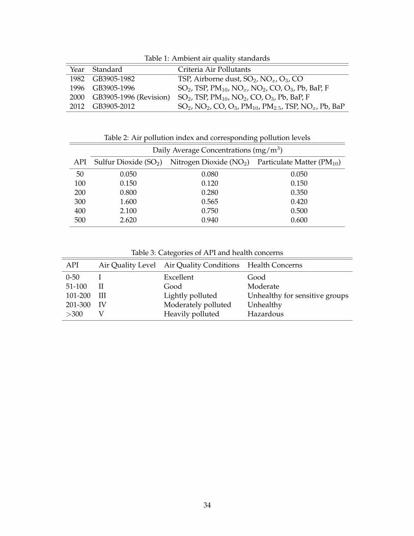
Table 1: Ambient air quality standardsYear Standard Criteria Air Pollutants1982 GB3905-1982 TSP, Airborne dust, SO2, NOx, O3, CO1996 GB3905-1996 SO2, TSP, PM10, NOx, NO2, CO, O3, Pb, BaP, F2000 GB3905-1996 (Revision) SO2, TSP, PM10, NO2, CO, O3, Pb, BaP, F2012 GB3905-2012 SO2, NO2, CO, O3, PM10, PM2.5, TSP, NOx, Pb, BaP
Table 2: Air pollution index and corresponding pollution levels
Daily Average Concentrations (mg/m3)
API Sulfur Dioxide (SO2) Nitrogen Dioxide (NO2) Particulate Matter (PM10)
50 0.050 0.080 0.050100 0.150 0.120 0.150200 0.800 0.280 0.350300 1.600 0.565 0.420400 2.100 0.750 0.500500 2.620 0.940 0.600
Table 3: Categories of API and health concerns
API Air Quality Level Air Quality Conditions Health Concerns
0-50 I Excellent Good51-100 II Good Moderate101-200 III Lightly polluted Unhealthy for sensitive groups201-300 IV Moderately polluted Unhealthy>300 V Heavily polluted Hazardous
34

Table 4: Summary statistics of the variables used in the analysisMean Std Min Max
API (max) 76.315 37.680 0 625Primary PollutantSO2 0.092NO2 0.002PM10 0.737GradeI 0.169II 0.677III1 0.124III2 0.021IV1 0.003IV2 0.002V 0.004Pollution Concentration (mg/m3)SO2 0.054 0.055 0.001 2.147NO2 0.036 0.020 0.001 0.353PM10 0.100 0.066 0.001 2.721API (pollutant level)SO2 43.262 27.544 0 409NO2 22.850 14.116 0 226PM10 74.731 38.277 0 501WeatherVisibility (VSB) 6.497 2.541 0 10Wind speed (SPD) 5.289 2.886 0 42.75Temperature (TEMP) 59.081 19.604 -23.50 98.04Pressure (STP) 965.954 76.455 637.78 1045.48Precipitation (PCP) 0.069 0.263 0 11.30
35

Table 5: t-Statistics for McCrary Test: Cities Exhibiting Manipulation (PM10)
a a10 15 20 10 15 2
Shenyang -10.318 -12.514 -14.091 Quanzhou -3.012 -3.414 -4.043Shijiazhuang -8.620 -10.609 -11.865 Zaozhuang -1.700 -3.330 -3.975Anshan -7.612 -8.748 -9.528 Nantong -2.285 -3.160 -3.145Beijing -7.800 -8.673 -9.064 Dalian -2.372 -2.998 -3.742Chengdu -6.407 -8.588 -10.079 Changzhi -2.548 -2.992 -3.156Nanjing -7.291 -8.277 -8.862 Anyang -3.075 -2.992 -3.161Hefei -6.648 -8.275 -9.239 Lanzhou -2.069 -2.931 -4.144Hangzhou -6.235 -7.735 -8.441 Weifang -0.821 -2.833 -4.159Xining -5.286 -6.294 -6.984 Datong -2.935 -2.803 -2.693Weinan -4.828 -6.144 -6.899 Jinan -1.356 -2.757 -3.841Changchun -3.602 -5.541 -6.750 Zhenjiang -1.512 -2.697 -3.553Luoyang -5.198 -5.409 -5.307 Guiyang -2.226 -2.413 -2.327Chongqing -4.167 -5.307 -5.761 Yinchuan -1.806 -2.045 -2.541Jinzhou -4.054 -5.275 -5.728 Baoji -1.367 -1.979 -2.590Tianjin -3.759 -4.725 -5.510 Deyang -1.063 -1.975 -2.406Kaifeng -3.604 -4.663 -5.622 Xianyang -0.467 -1.930 -2.966Xiangtan -3.514 -4.649 -5.437 Yanan -1.282 -1.882 -2.202Qingdao -3.300 -4.625 -4.985 Rizhao -1.545 -1.841 -2.214Suzhou -3.066 -4.609 -5.728 Mianyang -1.671 -1.803 -1.935Xuzhou -3.301 -4.133 -4.539 Lianyungang -0.757 -1.738 -2.194Guiyang -3.072 -3.982 -4.812 Yangquan -1.731 -1.736 -1.524Changzhou -3.574 -3.905 -4.079 Shenzhen -0.572 -1.656 -2.540Baotou -2.856 -3.829 -4.532 Nanchang -0.858 -1.633 -2.358Taiyuan -2.833 -3.820 -5.254 Tongchuan -0.581 -1.576 -1.859Linfen -3.466 -3.803 -4.056 Luzhou -1.671 -1.620 -1.278Xian -1.848 -3.672 -4.914 Taian -0.681 -1.572 -2.472Wulumuqi -3.582 -3.672 -4.269 Yantai -0.873 -1.288 -1.879Wuhan -3.242 -3.534 -3.355 Yangzhou -0.673 -1.237 -1.663Guangzhou -3.113 -3.497 -3.324 Lasa -0.711 -1.099 -1.678Jining -2.109 -3.475 -3.973 Shaoxing -1.030 -1.544 -1.463
Huhehaote -1.066 -1.325 -1.614
This table reports the McCrary t-statistic for each city using the PM10 concentration data.Notes: a = h/b̂, h is the bandwidth and b̂ = 2σ̂/
√n, where σ̂ is the standard deviation of the
pollutant concentration. For more details, please see Appendix A.
36
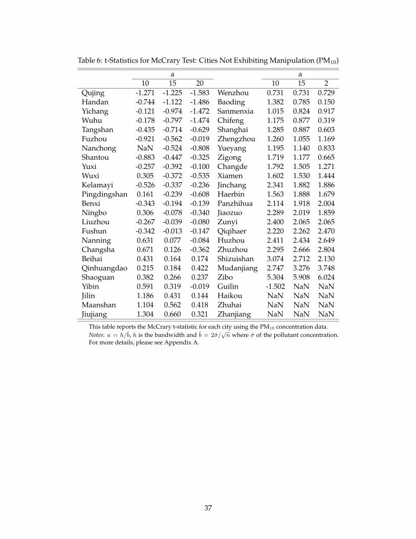
Table 6: t-Statistics for McCrary Test: Cities Not Exhibiting Manipulation (PM10)
a a10 15 20 10 15 2
Qujing -1.271 -1.225 -1.583 Wenzhou 0.731 0.731 0.729Handan -0.744 -1.122 -1.486 Baoding 1.382 0.785 0.150Yichang -0.121 -0.974 -1.472 Sanmenxia 1.015 0.824 0.917Wuhu -0.178 -0.797 -1.474 Chifeng 1.175 0.877 0.319Tangshan -0.435 -0.714 -0.629 Shanghai 1.285 0.887 0.603Fuzhou -0.921 -0.562 -0.019 Zhengzhou 1.260 1.055 1.169Nanchong NaN -0.524 -0.808 Yueyang 1.195 1.140 0.833Shantou -0.883 -0.447 -0.325 Zigong 1.719 1.177 0.665Yuxi -0.257 -0.392 -0.100 Changde 1.792 1.505 1.271Wuxi 0.305 -0.372 -0.535 Xiamen 1.602 1.530 1.444Kelamayi -0.526 -0.337 -0.236 Jinchang 2.341 1.882 1.886Pingdingshan 0.161 -0.239 -0.608 Haerbin 1.563 1.888 1.679Benxi -0.343 -0.194 -0.139 Panzhihua 2.114 1.918 2.004Ningbo 0.306 -0.078 -0.340 Jiaozuo 2.289 2.019 1.859Liuzhou -0.267 -0.039 -0.080 Zunyi 2.400 2.065 2.065Fushun -0.342 -0.013 -0.147 Qiqihaer 2.220 2.262 2.470Nanning 0.631 0.077 -0.084 Huzhou 2.411 2.434 2.649Changsha 0.671 0.126 -0.362 Zhuzhou 2.295 2.666 2.804Beihai 0.431 0.164 0.174 Shizuishan 3.074 2.712 2.130Qinhuangdao 0.215 0.184 0.422 Mudanjiang 2.747 3.276 3.748Shaoguan 0.382 0.266 0.237 Zibo 5.304 5.908 6.024Yibin 0.591 0.319 -0.019 Guilin -1.502 NaN NaNJilin 1.186 0.431 0.144 Haikou NaN NaN NaNMaanshan 1.104 0.562 0.418 Zhuhai NaN NaN NaNJiujiang 1.304 0.660 0.321 Zhanjiang NaN NaN NaN
This table reports the McCrary t-statistic for each city using the PM10 concentration data.Notes: a = h/b̂, h is the bandwidth and b̂ = 2σ̂/
√n where σ̂ of the pollutant concentration.
For more details, please see Appendix A.
37

Table 7: t-Statistics for McCrary Test: CitiesExhibiting Manipulation of SO2
a10 15 20
Shijiazhuang -4.9154 -5.4971 -5.7896Anshan -4.3499 -5.1613 -5.5384Yangquan -3.7741 -4.7820 -5.4176Zunyi -3.1786 -4.6268 -5.1011Tangshan -2.8904 -3.8594 -4.2408Linfen -2.7670 -3.5816 -3.1446Weifang -2.1114 -3.1647 -4.0624Handan -3.4122 -3.0500 -2.6932Shizuishan -2.2226 -2.9100 -3.5842Taiyuan -1.2444 -2.7966 -3.9241Dalian -2.7057 -2.6835 -2.6973Tianjin -1.6428 -2.4047 -2.3984Zhengzhou -1.4686 -2.1941 -2.6340Kunming -1.9936 -2.1755 -2.0017Guiyang -1.5683 -2.0856 -2.5199Baoding -1.3858 -1.8321 -2.2295Jinzhou -1.3630 -1.7740 -1.7233Kaifeng -0.5515 -1.7361 -1.6730Baotou -1.4601 -1.6942 -1.7832Wulumuqi -1.3142 -1.5663 -1.9597Changzhi -1.0818 -1.4499 -1.6063Shenyang -0.3135 -1.3845 -2.1399Jinan -0.9440 -1.3724 -1.2364Zaozhuang -1.3397 -1.3693 -1.3118Datong -1.3776 -1.3352 -0.4627Weinan -0.4897 -1.3234 -2.0854
This table reports the McCrary t-statistic for eachcity using the SO2 concentration data.Notes: a = h/b̂, h is the bandwidth and b̂ =2σ̂/
√n where σ̂ of the pollutant concentration.
For more details, please see Appendix A.
38

Table 8: t-Statistics for McCrary Test: NO2
a a10 15 20 10 15 2
Guangzhou -3.516 -3.409 -3.824 Hangzhou 1.034 0.115 -0.664Mudanjiang -3.237 -3.222 -3.152 Xianyang NaN 0.150 0.379Shenzhen -2.502 -3.145 -3.678 Weinan 0.996 0.174 -0.283Luoyang -1.666 -2.247 -2.237 Changzhi 0.034 0.360 0.388Yinchuan NaN -1.741 -6.336 Lanzhou 0.795 0.409 0.046Anyang -1.850 -1.562 -1.451 Shijiazhuang 1.074 0.418 0.657Kaifeng -1.392 -1.402 -1.276 Xiamen -2.523 0.475 0.259Nanning NaN -1.318 -1.252 Nanjing 0.987 0.547 0.263Beijing -1.425 -1.314 -1.378 Wuhan 0.848 0.558 0.309Fushun NaN -1.207 -1.300 Linfen 0.311 0.741 0.474Ningbo -0.929 -1.140 -1.275 Tianjin 0.524 0.871 1.029Haerbin -1.775 -1.104 -0.692 Chongqing 1.067 0.921 0.643Wuxi NaN -1.000 -2.413 Huhehaote 0.890 1.121 1.440Huzhou -0.518 -0.732 -0.741 Yangquan NaN 1.135 0.789Xuzhou NaN -0.357 Inf Datong 0.366 1.200 1.326Wenzhou 0.217 -0.351 -0.248 Suzhou 0.717 1.213 1.659Zhenjiang NaN -0.042 NaN Baoding 1.300 1.255 1.381Wuhu NaN -0.042 0.000 Zigong 1.401 1.324 1.375Zunyi NaN 0.000 0.000 Jiaozuo 1.071 1.502 1.398Pingdingshan 0.000 0.000 0.281 Yanan 0.371 1.730 2.198Yueyang 0.000 0.000 1.158 Shanghai 2.068 1.790 1.589Benxi 0.000 0.000 -0.595 Wulumuqi 1.278 1.799 1.843Shenyang 0.000 0.000 0.000 Handan 1.496 1.883 2.164Changde NaN 0.000 0.000 Nantong -4.747 1.939 2.249Panzhihua NaN 0.005 0.846
This table reports the McCrary t-statistic for each city using the NO2 concentration data.Notes: a = h/b̂, h is the bandwidth and b̂ = 2σ̂/
√n where σ̂ of the pollutant concentration. For
more details, please see Appendix A.
39

Table 9: McCrary test: Comparison between Concentra-tion and API Results
Concentration APINo. of Manipulators (α = 0.05)PM10 52 50SO2 19 4NO2 5 7Ranking (PM10)Beijing 4 7Chongqing 13 15Shanghai 91 95Tianjin 15 26
This table reports the difference in the results betweenusing pollutant concentration versus API in the Mc-Crary test.
40

Table 10: PMA-McCrary Comparison
City-pair PMA McCrary (2008)Rejections City 1 City 2
Zhenjiang-Yangzhou NO Borderline NOChangzhou-Wuxi NO YES NOJilin-Changchun NO NO YESKaifeng-Zhengzhou YES YES NOZhuzhou-Xiangtan YES NO YESQuanzhou-Xiamen YES YES NOHangzhou-Shaoxing YES NO NOShenyang-Fushun YES YES NOYinchuan-Shizuishan YES Borderline NOXian-Xianyang YES YES BorderlineJinan-Taian YES YES NOHuhehaote-Baotou YES NO YESWuhu-Maanshan NO NO NO
The table compares the results from the panel matching ap-proach (PMA) with the McCrary (2008) test. YES indicatesthat there was evidence of manipulation, NO indicates thatthere was no evidence of manipulation, and Borderline indi-cates that there is borderline evidence of manipulation. Forinstance, it was a borderline p-value at the 5% level.
41

Beijing
API
Den
sity
0 50 100 150 200
0.00
00.
015
0.03
0
I II III1 III2
Tianjin
API
Den
sity
0 50 100 150 200
0.00
00.
015
0.03
0
I II III1 III2
Shanghai
API
Den
sity
0 50 100 150 200
0.00
00.
015
0.03
0
I II III1 III2
Chongqing
API
Den
sity
0 50 100 150 200
0.00
00.
015
0.03
0
I II III1 III2
Figure 1: Frequency of API scores in four capital cities: Beijing (upper left), Tianjin (upper right),Shanghai (lower left), and Chongqing (lower right). The histograms are based on the city-leveldaily API scores during 2001-2010. Scores greater than 200 are not illustrated. The red lines denotethe cut-off points for each pollution level. Levels I and II are defined as ”blue-sky days.”
42
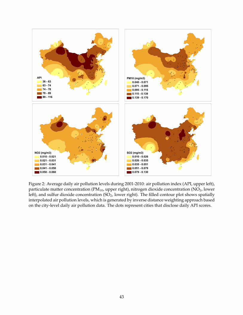
!
!
!
!
!
!
!
!
!
!
!!
!!
!!
!
!
!
!
!
!!
!
!
!
!!
!
!
!!
!
!
!!
! !
!
!
!
!!
!
!
!
!
!
!
! !!
!
!
!
!
!
!
! !!
!
!
!
!
!!!
!
!!!
!
!
!
!
!
!
!
!
!
!
!
!
!
!
!!
!
!
!!
!
! !
!
!
!
!
!
!
!
! !!
!
!
!
!
!
!
!
!
API36 - 6363 - 7474 - 7878 - 8989 - 116
!
!
!
!
!
!
!
!
!
!
!!
!!
!!
!
!
!
!
!
!!
!
!
!
!!
!
!
!!
!
!
!!
! !
!
!
!
!!
!
!
!
!
!
!
! !!
!
!
!
!
!
!
! !!
!
!
!
!
!!!
!
!!!
!
!
!
!
!
!
!
!
!
!
!
!
!
!
!!
!
!
!!
!
! !
!
!
!
!
!
!
!
! !!
!
!
!
!
!
!
!
!
PM10 (mg/m3)0.040 - 0.0710.071 - 0.0950.095 - 0.1150.115 - 0.1390.139 - 0.170
!
!
!
!
!
!
!
!
!
!
!!
!!
!!
!
!
!
!
!
!!
!
!
!
!!
!
!
!!
!
!
!!
! !
!
!
!
!!
!
!
!
!
!
!
! !!
!
!
!
!
!
!
! !!
!
!
!
!
!!!
!
!!!
!
!
!
!
!
!
!
!
!
!
!
!
!
!
!!
!
!
!!
!
! !
!
!
!
!
!
!
!
! !!
!
!
!
!
!
!
!
!
NO2 (mg/m3)0.010 - 0.0210.021 - 0.0310.031 - 0.0410.041 - 0.0500.050 - 0.060
!
!
!
!
!
!
!
!
!
!
!!
!!
!!
!
!
!
!
!
!!
!
!
!
!!
!
!
!!
!
!
!!
! !
!
!
!
!!
!
!
!
!
!
!
! !!
!
!
!
!
!
!
! !!
!
!
!
!
!!!
!
!!!
!
!
!
!
!
!
!
!
!
!
!
!
!
!
!!
!
!
!!
!
! !
!
!
!
!
!
!
!
! !!
!
!
!
!
!
!
!
!
SO2 (mg/m3)0.010 - 0.0260.026 - 0.0350.035 - 0.0510.051 - 0.0790.079 - 0.130
Figure 2: Average daily air pollution levels during 2001-2010: air pollution index (API, upper left),particulate matter concentration (PM10, upper right), nitrogen dioxide concentration (NO2, lowerleft), and sulfur dioxide concentration (SO2, lower right). The filled contour plot shows spatiallyinterpolated air pollution levels, which is generated by inverse distance weighting approach basedon the city-level daily air pollution data. The dots represent cities that disclose daily API scores.
43

0 0.1 0.2 0.3 0.4 0.5 0.6 0.7 0.8 0.9 10
50
100
150
200
Concentration (mg/m3)
AP
I
SO2
NO2
PM10
Figure 3: API is a nonlinear transformation of pollutant concentrations. In particular, there arekinks corresponding to API=100 for SO2 and NO2 respectively
44

McCrary Test Resultst-stat
-12.51 - -2.00-1.99 - -1.50-1.49 - 5.91No Data
Figure 4: Results of McCrary (2008) tests show different degrees of manipulation in the PM10
data. Three levels of manipulation are illustrated: t-stats below -1.5 as non-manipulators, t-statsbetween -1.5 and -2 as borderline manipulators, and finally, t-stats smaller than -2 as manipulators.PM10 is selected because it is the dominant primary pollutant. A polygon is a prefecture that hasthe city as its capital.
45
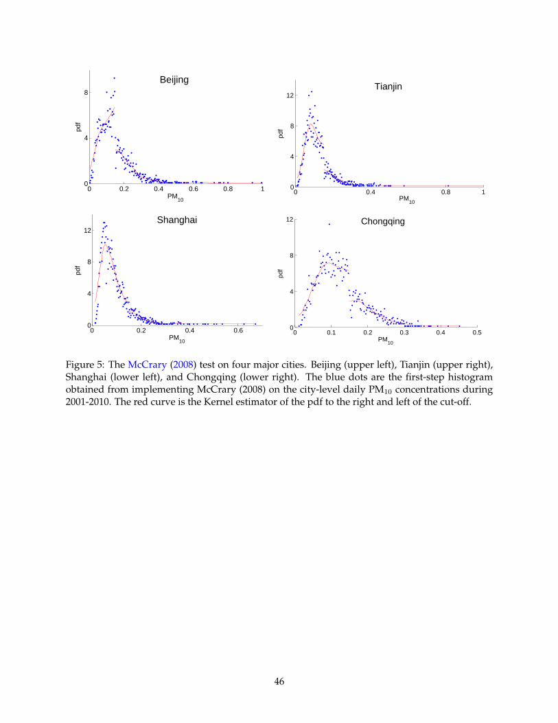
0 0.2 0.4 0.6 0.8 10
4
8
PM10
Beijing
0 0.4 0.8 10
4
8
12
PM10
Tianjin
0 0.2 0.4 0.60
4
8
12
PM10
Shanghai
0 0.1 0.2 0.3 0.4 0.50
4
8
12
PM10
Chongqing
Figure 5: The McCrary (2008) test on four major cities. Beijing (upper left), Tianjin (upper right),Shanghai (lower left), and Chongqing (lower right). The blue dots are the first-step histogramobtained from implementing McCrary (2008) on the city-level daily PM10 concentrations during2001-2010. The red curve is the Kernel estimator of the pdf to the right and left of the cut-off.
46

PM10
−2 0 2 4
−10
−5
0
5
10
GDP per capita (log)
McC
rary
t−st
atis
tic
2 4 6 8
−10
−5
0
5
10
Population Density (log)
McC
rary
t−st
atis
tic
−2 0 2 4
−10
−5
0
5
10
Industrial VA per capita (log)
McC
rary
t−st
atis
tic
SO2
−1 0 1 2 3
−10
−6
−2
2
6
GDP per capita (log)
McC
rary
t−st
atis
tic
2 4 6 8
−10
−6
−2
2
6
Population Density (log)
McC
rary
t−st
atis
tic
−2 −1 0 1 2
−10
−6
−2
2
6
Industrial VA per capita (log)
McC
rary
t−st
atis
tic
NO2
0 1 2 3 4
−10
−6
−2
2
6
GDP per capita (log)
McC
rary
t−st
atis
tic
4 5 6 7 8
−10
−6
−2
2
6
Population Density (log)
McC
rary
t−st
atis
tic
−2 0 2 4
−10
−6
−2
2
6
Industrial VA per capita (log)
McC
rary
t−st
atis
tic
Figure 6: GDP per capita, population density, industrial value added per capita and McCraryresults. The scatter plots graph the relationship between the log of GDP per capita (column 1), logof population density (column 2), log of value added of the secondary industry per capita (column3) and the McCrary t-statistics for PM10 (upper), SO2 (middle), and NO2 (lower).
47

API Visibility
Air QualityManipulation
Observable
Unobservable
Nature
Figure 7: An illustration of the identification assumptions in the panel matching approach.
48

50 100 1500
0.2
0.4
0.6
0.8
1
VSB=3, SPD=5, TEMP=80
EC
DF
of A
PI
50 100 1500
0.2
0.4
0.6
0.8
1
VSB=4, SPD=5, TEMP=80
EC
DF
of A
PI
50 100 1500
0.2
0.4
0.6
0.8
1
VSB=5, SPD=5, TEMP=80
EC
DF
of A
PI
50 100 1500
0.2
0.4
0.6
0.8
1
VSB=6, SPD=10, TEMP=80
EC
DF
of A
PI
50 100 1500
0.2
0.4
0.6
0.8
1
VSB=7, SPD=10, TEMP=40
EC
DF
of A
PI
50 100 1500
0.2
0.4
0.6
0.8
1
VSB=7, SPD=10, TEMP=100
EC
DF
of A
PI
Figure 8: Panel Matching Approach: Zhenjiang-Yangzhou. The red lines represent Zhenjiang,the blue Yangzhou. The solid lines are the empirical cdfs of API conditional on the weather vari-ables specified in the plot, the dotted lines give 95% point-wise confidence intervals for the em-pirical cdf. VSB denotes visibility, WSP wind speed, and TEMP temperature. The values for theweather variables are the discretized versions of the actual data for details on the discretizationsee Appendix C.
49

50 100 150 2000
0.2
0.4
0.6
0.8
1
VSB=4, SPD=5, TEMP=60
EC
DF
of A
PI
50 100 150 2000
0.2
0.4
0.6
0.8
1
VSB=5, SPD=5, TEMP=60
EC
DF
of A
PI
50 100 150 2000
0.2
0.4
0.6
0.8
1
VSB=6, SPD=5, TEMP=60
EC
DF
of A
PI
50 100 150 2000
0.2
0.4
0.6
0.8
1
VSB=7, SPD=5, TEMP=40
EC
DF
of A
PI
50 100 150 2000
0.2
0.4
0.6
0.8
1
VSB=7, SPD=5, TEMP=60
EC
DF
of A
PI
50 100 150 2000
0.2
0.4
0.6
0.8
1
VSB=7, SPD=10, TEMP=80
EC
DF
of A
PI
Figure 9: Panel Matching Approach: Changzhou-Wuxi. The red lines represent Changzhou, theblue Wuxi. The solid lines are the empirical cdfs of API conditional on the weather variables spec-ified in the plot, the dotted lines give 95% point-wise confidence intervals for the empirical cdf.VSB denotes visibility, WSP wind speed, and TEMP temperature. The values for the weather vari-ables are the discretized versions of the actual data for details on the discretization see AppendixC.
50

50 100 150 2000
0.2
0.4
0.6
0.8
1
VSB=3, SPD=5, TEMP=20
EC
DF
of A
PI
50 100 150 2000
0.2
0.4
0.6
0.8
1
VSB=4, SPD=5, TEMP=20
EC
DF
of A
PI
50 100 150 2000
0.2
0.4
0.6
0.8
1
VSB=5, SPD=10, TEMP=20
EC
DF
of A
PI
50 100 150 2000
0.2
0.4
0.6
0.8
1
VSB=6, SPD=10, TEMP=20
EC
DF
of A
PI
50 100 150 2000
0.2
0.4
0.6
0.8
1
VSB=7, SPD=5, TEMP=80
EC
DF
of A
PI
50 100 150 2000
0.2
0.4
0.6
0.8
1
VSB=7, SPD=10, TEMP=80
EC
DF
of A
PI
Figure 10: Panel Matching Approach: Jilin-Changchun. The red lines represent Jilin, the blueChangchun. The solid lines are the empirical cdfs of API conditional on the weather variablesspecified in the plot, the dotted lines give 95% point-wise confidence intervals for the empiricalcdf. VSB denotes visibility, WSP wind speed, and TEMP temperature. The values for the weathervariables are the discretized versions of the actual data for details on the discretization see Ap-pendix C.
51
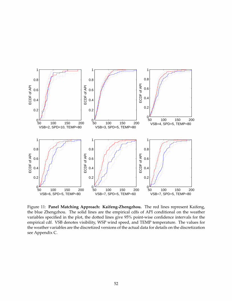
50 100 150 2000
0.2
0.4
0.6
0.8
1
VSB=2, SPD=10, TEMP=80
EC
DF
of A
PI
50 100 150 2000
0.2
0.4
0.6
0.8
1
VSB=3, SPD=5, TEMP=80
EC
DF
of A
PI
50 100 150 2000
0.2
0.4
0.6
0.8
1
VSB=4, SPD=5, TEMP=80
EC
DF
of A
PI
50 100 150 2000
0.2
0.4
0.6
0.8
1
VSB=6, SPD=5, TEMP=80
EC
DF
of A
PI
50 100 150 2000
0.2
0.4
0.6
0.8
1
VSB=7, SPD=5, TEMP=60
EC
DF
of A
PI
50 100 150 2000
0.2
0.4
0.6
0.8
1
VSB=7, SPD=5, TEMP=80
EC
DF
of A
PI
Figure 11: Panel Matching Approach: Kaifeng-Zhengzhou. The red lines represent Kaifeng,the blue Zhengzhou. The solid lines are the empirical cdfs of API conditional on the weathervariables specified in the plot, the dotted lines give 95% point-wise confidence intervals for theempirical cdf. VSB denotes visibility, WSP wind speed, and TEMP temperature. The values forthe weather variables are the discretized versions of the actual data for details on the discretizationsee Appendix C.
52

50 100 150 2000
0.2
0.4
0.6
0.8
1
VSB=2, SPD=10, TEMP=80
EC
DF
of A
PI
50 100 150 2000
0.2
0.4
0.6
0.8
1
VSB=3, SPD=5, TEMP=80
EC
DF
of A
PI
50 100 150 2000
0.2
0.4
0.6
0.8
1
VSB=4, SPD=5, TEMP=80
EC
DF
of A
PI
50 100 150 2000
0.2
0.4
0.6
0.8
1
VSB=6, SPD=5, TEMP=80
EC
DF
of A
PI
50 100 150 2000
0.2
0.4
0.6
0.8
1
VSB=7, SPD=5, TEMP=60
EC
DF
of A
PI
50 100 150 2000
0.2
0.4
0.6
0.8
1
VSB=7, SPD=5, TEMP=80
EC
DF
of A
PI
Figure 12: Panel Matching Approach: Zhuzhou-Xiangtan. The red lines represent Zhuzhou, theblue Xiangtan. The solid lines are the empirical cdfs of API conditional on the weather variablesspecified in the plot, the dotted lines give 95% point-wise confidence intervals for the empiricalcdf. VSB denotes visibility, WSP wind speed, and TEMP temperature. The values for the weathervariables are the discretized versions of the actual data for details on the discretization see Ap-pendix C.
53
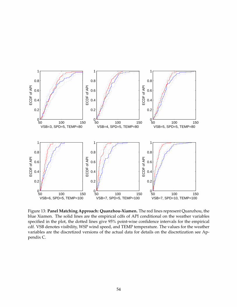
50 100 1500
0.2
0.4
0.6
0.8
1
VSB=3, SPD=5, TEMP=80
EC
DF
of A
PI
50 100 1500
0.2
0.4
0.6
0.8
1
VSB=4, SPD=5, TEMP=80
EC
DF
of A
PI
50 100 1500
0.2
0.4
0.6
0.8
1
VSB=5, SPD=5, TEMP=80
EC
DF
of A
PI
50 100 1500
0.2
0.4
0.6
0.8
1
VSB=6, SPD=5, TEMP=100
EC
DF
of A
PI
50 100 1500
0.2
0.4
0.6
0.8
1
VSB=7, SPD=5, TEMP=100
EC
DF
of A
PI
50 100 1500
0.2
0.4
0.6
0.8
1
VSB=7, SPD=10, TEMP=100
EC
DF
of A
PI
Figure 13: Panel Matching Approach: Quanzhou-Xiamen. The red lines represent Quanzhou, theblue Xiamen. The solid lines are the empirical cdfs of API conditional on the weather variablesspecified in the plot, the dotted lines give 95% point-wise confidence intervals for the empiricalcdf. VSB denotes visibility, WSP wind speed, and TEMP temperature. The values for the weathervariables are the discretized versions of the actual data for details on the discretization see Ap-pendix C.
54

50 100 1500
0.2
0.4
0.6
0.8
1
VSB=1, SPD=5, TEMP=60
EC
DF
of A
PI
50 100 1500
0.2
0.4
0.6
0.8
1
VSB=2, SPD=5, TEMP=60
EC
DF
of A
PI
50 100 1500
0.2
0.4
0.6
0.8
1
VSB=4, SPD=10, TEMP=80
EC
DF
of A
PI
50 100 1500
0.2
0.4
0.6
0.8
1
VSB=5, SPD=5, TEMP=80
EC
DF
of A
PI
50 100 1500
0.2
0.4
0.6
0.8
1
VSB=6, SPD=5, TEMP=100
EC
DF
of A
PI
50 100 1500
0.2
0.4
0.6
0.8
1
VSB=6, SPD=10, TEMP=100
EC
DF
of A
PI
Figure 14: Panel Matching Approach: Hangzhou-Shaoxing. The red lines represent Hangzhou,the blue Shaoxing. The solid lines are the empirical cdfs of API conditional on the weather vari-ables specified in the plot, the dotted lines give 95% point-wise confidence intervals for the em-pirical cdf. VSB denotes visibility, WSP wind speed, and TEMP temperature. The values for theweather variables are the discretized versions of the actual data for details on the discretizationsee Appendix C.
55

50 100 150 2000
0.2
0.4
0.6
0.8
1
VSB=4, SPD=5, TEMP=20
EC
DF
of A
PI
50 100 150 2000
0.2
0.4
0.6
0.8
1
VSB=4, SPD=5, TEMP=80
EC
DF
of A
PI
50 100 150 2000
0.2
0.4
0.6
0.8
1
VSB=5, SPD=5, TEMP=80
EC
DF
of A
PI
50 100 150 2000
0.2
0.4
0.6
0.8
1
VSB=6, SPD=5, TEMP=80
EC
DF
of A
PI
50 100 150 2000
0.2
0.4
0.6
0.8
1
VSB=7, SPD=5, TEMP=80
EC
DF
of A
PI
50 100 150 2000
0.2
0.4
0.6
0.8
1
VSB=7, SPD=10, TEMP=80
EC
DF
of A
PI
Figure 15: Panel Matching Approach: Shenyang-Fushun. The red lines represent Shenyang, theblue Fushun. The solid lines are the empirical cdfs of API conditional on the weather variablesspecified in the plot, the dotted lines give 95% point-wise confidence intervals for the empiricalcdf. VSB denotes visibility, WSP wind speed, and TEMP temperature. The values for the weathervariables are the discretized versions of the actual data for details on the discretization see Ap-pendix C.
56

50 100 150 2000
0.2
0.4
0.6
0.8
1
VSB=7, SPD=5, TEMP=20
EC
DF
of A
PI
50 100 150 2000
0.2
0.4
0.6
0.8
1
VSB=7, SPD=5, TEMP=40
EC
DF
of A
PI
50 100 150 2000
0.2
0.4
0.6
0.8
1
VSB=7, SPD=5, TEMP=80
EC
DF
of A
PI
50 100 150 2000
0.2
0.4
0.6
0.8
1
VSB=7, SPD=10, TEMP=40
EC
DF
of A
PI
50 100 150 2000
0.2
0.4
0.6
0.8
1
VSB=7, SPD=10, TEMP=60
EC
DF
of A
PI
50 100 150 2000
0.2
0.4
0.6
0.8
1
VSB=7, SPD=10, TEMP=80
EC
DF
of A
PI
Figure 16: Panel Matching Approach: Yinchuan-Shizuishan. The red lines represent Yinchuan,the blue Shizuishan. The solid lines are the empirical cdfs of API conditional on the weathervariables specified in the plot, the dotted lines give 95% point-wise confidence intervals for theempirical cdf. VSB denotes visibility, WSP wind speed, and TEMP temperature. The values forthe weather variables are the discretized versions of the actual data for details on the discretizationsee Appendix C.
57

50 100 150 2000
0.2
0.4
0.6
0.8
1
VSB=2, SPD=5, TEMP=60
EC
DF
of A
PI
50 100 150 2000
0.2
0.4
0.6
0.8
1
VSB=3, SPD=5, TEMP=40
EC
DF
of A
PI
50 100 150 2000
0.2
0.4
0.6
0.8
1
VSB=3, SPD=5, TEMP=60
EC
DF
of A
PI
50 100 150 2000
0.2
0.4
0.6
0.8
1
VSB=4, SPD=5, TEMP=60
EC
DF
of A
PI
50 100 150 2000
0.2
0.4
0.6
0.8
1
VSB=6, SPD=5, TEMP=80
EC
DF
of A
PI
50 100 150 2000
0.2
0.4
0.6
0.8
1
VSB=7, SPD=10, TEMP=100
EC
DF
of A
PI
Figure 17: Panel Matching Approach: Xian-Xianyang. The red lines represent Xian, the blue Xi-anyang. The solid lines are the empirical cdfs of API conditional on the weather variables specifiedin the plot, the dotted lines give 95% point-wise confidence intervals for the empirical cdf. VSBdenotes visibility, WSP wind speed, and TEMP temperature. The values for the weather variablesare the discretized versions of the actual data for details on the discretization see Appendix C.
58

50 100 1500
0.2
0.4
0.6
0.8
1
VSB=2, SPD=5, TEMP=80
EC
DF
of A
PI
50 100 1500
0.2
0.4
0.6
0.8
1
VSB=3, SPD=5, TEMP=80
EC
DF
of A
PI
50 100 1500
0.2
0.4
0.6
0.8
1
VSB=7, SPD=5, TEMP=60
EC
DF
of A
PI
50 100 1500
0.2
0.4
0.6
0.8
1
VSB=7, SPD=10, TEMP=40
EC
DF
of A
PI
50 100 1500
0.2
0.4
0.6
0.8
1
VSB=7, SPD=10, TEMP=60
EC
DF
of A
PI
50 100 1500
0.2
0.4
0.6
0.8
1
VSB=7, SPD=10, TEMP=80
EC
DF
of A
PI
Figure 18: Panel Matching Approach: Jinan-Taian. The red lines represent Jinan, the blue Taian.The solid lines are the empirical cdfs of API conditional on the weather variables specified in theplot, the dotted lines give 95% point-wise confidence intervals for the empirical cdf. VSB denotesvisibility, WSP wind speed, and TEMP temperature. The values for the weather variables are thediscretized versions of the actual data for details on the discretization see Appendix C.
59

50 100 150 2000
0.2
0.4
0.6
0.8
1
VSB=7, SPD=5, TEMP=40
EC
DF
of A
PI
50 100 150 2000
0.2
0.4
0.6
0.8
1
VSB=7, SPD=5, TEMP=80
EC
DF
of A
PI
50 100 150 2000
0.2
0.4
0.6
0.8
1
VSB=7, SPD=10, TEMP=20
EC
DF
of A
PI
50 100 150 2000
0.2
0.4
0.6
0.8
1
VSB=7, SPD=10, TEMP=60
EC
DF
of A
PI
50 100 150 2000
0.2
0.4
0.6
0.8
1
VSB=7, SPD=10, TEMP=80
EC
DF
of A
PI
50 100 150 2000
0.2
0.4
0.6
0.8
1
VSB=7, SPD=15, TEMP=80
EC
DF
of A
PI
Figure 19: Panel Matching Approach: Huhehaote-Baotou. The red lines represent Huhehaote,the blue Baotou. The solid lines are the empirical cdfs of API conditional on the weather variablesspecified in the plot, the dotted lines give 95% point-wise confidence intervals for the empiricalcdf. VSB denotes visibility, WSP wind speed, and TEMP temperature. The values for the weathervariables are the discretized versions of the actual data for details on the discretization see Ap-pendix C.
60
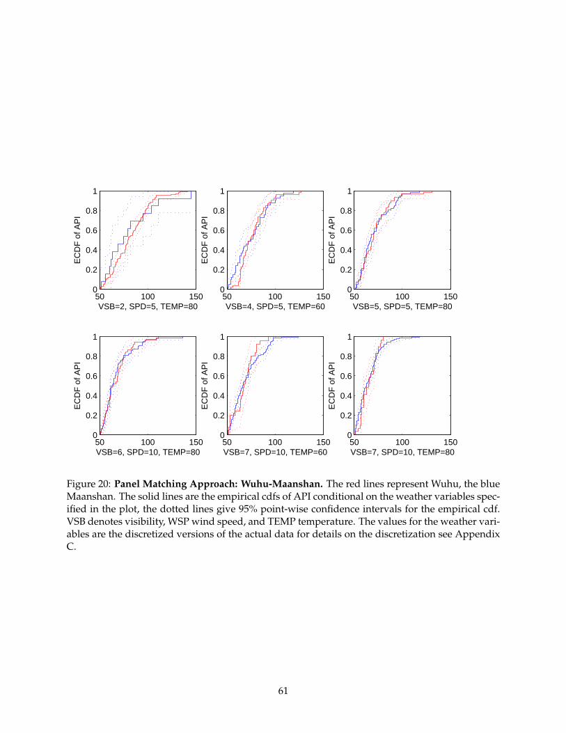
50 100 1500
0.2
0.4
0.6
0.8
1
VSB=2, SPD=5, TEMP=80
EC
DF
of A
PI
50 100 1500
0.2
0.4
0.6
0.8
1
VSB=4, SPD=5, TEMP=60
EC
DF
of A
PI
50 100 1500
0.2
0.4
0.6
0.8
1
VSB=5, SPD=5, TEMP=80
EC
DF
of A
PI
50 100 1500
0.2
0.4
0.6
0.8
1
VSB=6, SPD=10, TEMP=80
EC
DF
of A
PI
50 100 1500
0.2
0.4
0.6
0.8
1
VSB=7, SPD=10, TEMP=60
EC
DF
of A
PI
50 100 1500
0.2
0.4
0.6
0.8
1
VSB=7, SPD=10, TEMP=80
EC
DF
of A
PI
Figure 20: Panel Matching Approach: Wuhu-Maanshan. The red lines represent Wuhu, the blueMaanshan. The solid lines are the empirical cdfs of API conditional on the weather variables spec-ified in the plot, the dotted lines give 95% point-wise confidence intervals for the empirical cdf.VSB denotes visibility, WSP wind speed, and TEMP temperature. The values for the weather vari-ables are the discretized versions of the actual data for details on the discretization see AppendixC.
61
Top Related