


Languages
Pages
Legal

IOSR Journal of Engineering (IOSRJEN)
e-ISSN: 2250-3021, p-ISSN: 2278-8719, www.iosrjen.org Volume 2, Issue 9 (September 2012), PP 116-121
www.iosrjen.org 116 | P a g e
Effects of Fading Channels on OFDM
Ahmed Alshammari, Saleh Albdran, and Dr. Mohammad Matin Department of Electrical and Computer Engineering University of Denver
Abstract––One of the essential components of recent communications is Orthogonal Frequency Division
Multiplexing (OFDM). Handling bad conditions, high bandwidth and using the available spectral efficiently are
some of its characteristics. Hence, it has replaced old communication technologies in many systems such as
wireless networks and 4G mobile communications. In this paper, Effects of fading channels on OFDM are
investigated. MATLAB is used to simulate wireless fading channels environments that are either based on
Doppler spread or Delay Spread.
Key Words–– OFDM, ISI, BER, PSNRs
I. INTRODUCTION High data rates are demanded a lot in modern communications. It is the huge development in the
communications industry that led to this demand. Also, better quality and lower BER became more important.
OFDM technique, which was introduced in the 1960’s, provides all that [1][2]. It was not practical at that time
because technologies to apply did not exist then e.g. it was not possible to have processors that can perform
IFFT and FFT. In the 90’s many of those problems were solved and OFDM started getting more popular since
then.
Multi carrier modulation is the backbone of the OFDM technique. Hence, data are split to many
parallel streams, which decreases bit rate. OFDM system of modulates several subcarriers using these parallel
sub streams. OFDM’s ability to transmit data with high speed is the main reason it is getting so popular besides
robustness against Inter symbol interference (ISI). Therefore, many wireless and wired communication
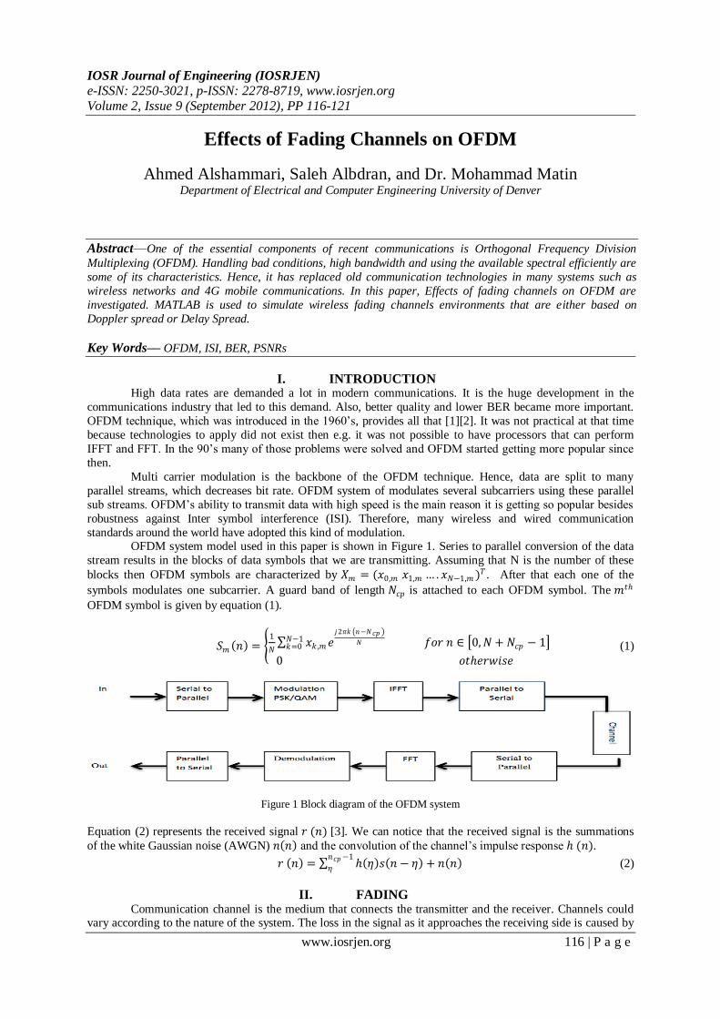
standards around the world have adopted this kind of modulation. OFDM system model used in this paper is shown in Figure 1. Series to parallel conversion of the data
stream results in the blocks of data symbols that we are transmitting. Assuming that N is the number of these
blocks then OFDM symbols are characterized by 𝑋𝑚 = (𝑥0,𝑚 𝑥1,𝑚 … . 𝑥𝑁−1,𝑚 )𝑇 . After that each one of the
symbols modulates one subcarrier. A guard band of length 𝑁𝑐𝑝 is attached to each OFDM symbol. The 𝑚𝑡ℎ
OFDM symbol is given by equation (1).
𝑆𝑚 𝑛 = 1
𝑁 𝑥𝑘 ,𝑚𝑒
𝑗2𝜋𝑘 𝑛−𝑁𝑐𝑝
𝑁𝑁−1𝑘=0 𝑓𝑜𝑟 𝑛 ∈ 0, 𝑁 + 𝑁𝑐𝑝 − 1
0 𝑜𝑡ℎ𝑒𝑟𝑤𝑖𝑠𝑒
(1)
Figure 1 Block diagram of the OFDM system
Equation (2) represents the received signal 𝑟 (𝑛) [3]. We can notice that the received signal is the summations
of the white Gaussian noise (AWGN) 𝑛 𝑛 and the convolution of the channel’s impulse response ℎ (𝑛).
𝑟 𝑛 = ℎ 𝜂 𝑠 𝑛 − 𝜂 + 𝑛 𝑛 𝑛𝑐𝑝 −1
𝜂 (2)
II. FADING Communication channel is the medium that connects the transmitter and the receiver. Channels could vary according to the nature of the system. The loss in the signal as it approaches the receiving side is caused by

Effects of Fading Channels on OFDM
www.iosrjen.org 117 | P a g e
random attenuations. In wireless environment, it is possible that signals propagate through two or more paths
before reaching the receiver in a phenomenon that is known as multipath propagation. There are many reasons
that can cause multipath such as atmospheric conditions or lack of direct bath. Phase shifting, destructive and constructive interference are some of the consequences of this phenomenon [4]. Hence, received signal could
have different amplitude and phase because of change in the propagation time and the intensity distribution of
the waves [5].
2.1 Small Scale Fading
Small scale fading is controlled by the nature of the sent signal and communication environments.
Symbol duration, Bandwidth and channel parameter are factors that decide the type of fading channel. Small
scale fading could be divided into two main categories as shown in figure 2:
1) Fading Due To Delay Spread: Delay spread can cause two types fading that are either frequency selective
slow and frequency selective fast fading [5]. Flat fading is the most popular types of fading. It occurs when the
bandwidth of the signal is less than the bandwidth of the channel. The power of the signal is reduced in this case as a consequence to the gain variation of the channel when the spectrum remains the same. In frequency
selective fading: linear phase response and constant gain are the main characteristics. Bandwidth of the channel
is smaller than that of the signal, which is distorted by frequency selective, fading due to the multiple version of
the signal with various amplitudes that are received.
2) Fading From Doppler Spread: it is either flat slow or flat fast fading caused by Doppler spread. In slow
fading, symbol period is more than coherence. In Fast Fading, impulse response of the channel variations are
very fast i.e. symbol duration of the transmitted signal is more than the coherence time.
Figure 2 Small Scale Fading
2.2 Factors affecting fading:
Four things could affect small scale fading:
1) Mobile speed: moving mobile could experience positive or negative Doppler shift. When the mobile
moves closer to the transmitting side positive Doppler spread happened while Negative Doppler spread
occurs the other way around. 2) Multipath Propagation: Signal energy is consumed by phase, amplitude and time in multipath
environment. Multiple versions of the signal with various arriving instants and shifted spatial orientation.
The duration that the signal takes to get to the receiver is increased in multipath channels.
3) Bandwidth of The Channel: When the bandwidth of the channel is less that that of the signal transmitted, it
gets distorted. The channel transfer function must be flat in order for its bandwidth to be coherent.
Transfer function of the channel is flat whenever the phase response is linear with a constant gain [6].

Effects of Fading Channels on OFDM
www.iosrjen.org 118 | P a g e
4) Velocity of objects within the channel: Objects in the communication environment sometimes are moving.
If that movement is of a speed that is more than that of the receiver, small-scale fading happens otherwise
we can ignore those movements.
III. CHANNEL MODELING Time variant impulse response of the channel is used to model it. Motion of the receiver is the variable
that affects time changing. Equation (3) is calculates the received signal.
𝑦 𝑑, 𝑡 = 𝑥 𝜏 ℎ 𝑑, 𝑡 − 𝜏 𝑑(𝑡)𝑡
−∞ (3)
Where ℎ (𝑑, 𝑡) is the impulse response of the channel and 𝑥 (𝑡) is the signal. If 𝑑 = 𝑣𝑡 is the position of the
receiver and 𝑣 is a constant, it is possible to replace 𝑑 in equation (3) with 𝑣𝑡 as in equation (4).
𝑦 𝑣𝑡, 𝑡 = 𝑥 𝜏 ℎ 𝑣𝑡, 𝑡 − 𝜏 𝑑(𝑡)𝑡
−∞ (4)
ℎ𝑏 𝑡, 𝜏 = 𝑎𝑖(𝑡, 𝜏)𝑒 𝑗 2𝜋𝑓𝑐𝜏𝑖 𝑡 +𝜑𝑖 𝑡,𝜏 𝛿(𝜏 − 𝜏𝑖 𝑡 )𝑁−1𝑖=0 (8)
Channel impulse response can be found using (5). Where, 𝑎𝑖(𝑡, 𝜏) are the amplitudes and 𝜏𝑖(𝑡) are the delays
whereas 𝜃𝑖 𝑡, 𝜏 = 2𝜋𝑓𝑐𝜏𝑖 𝑡 + 𝜑𝑖 𝑡, 𝜏 represent phase shift in the 𝑖th component.
The impulse response can be found using equation (9) for time invariant channel where every multipath
components of that cannel have delay.
ℎ𝑏 𝜏 = 𝑎𝑖(𝑡, 𝜏)𝑒 𝑗𝜃 𝑖 𝑡 ,𝜏 𝛿(𝜏 − 𝜏𝑖 𝑡 )𝑁−1𝑖=0 (9)
3.1 Clarke’s Model
Clarke’s Model relies on scattering to discover the statistical characteristics of the channel. Beside the
assumption of fixed transmission antenna that is vertically polarized, N normalized plane waves of the antenna with a random carrier phases angels of arrival are assumed while amplitude remains unchanged. When the
receiver is moving, 𝑚𝑡ℎ wave that has arriving angle 𝛼𝑚 with respect to the x-axis. Doppler shift is given by
equation (10).
𝑓𝑚 =𝑣
𝜆𝑐𝑜𝑠𝛼𝑚 (10)
Where, 𝜆 is the wavelength of incident wave.
Every received wave has a different carrier frequency with small shift from the center frequency. The
power spectral density of the output is given by equation 11. It is clear from that equation that the PDF is zero
when 𝑓 − 𝑓𝑐 > 𝑓𝑚 . With center frequency 𝑓𝑐 , Spectrum is limited to ±𝑓𝑚 and all the received waves has
different carrier frequencies that are shifted.
𝑆 𝑓 =𝐴[𝑞 𝛼 𝐺 ∝ + −∝ 𝐺(−∝)
𝑓𝑛 1−(𝑓−𝑓𝑐𝑓𝑚
)2 (11)
Assuming a vertical 𝜆
4 antenna, 𝐺 𝛼 = 1.5 and 𝑝 𝛼 =
1
2𝜋 over 0 to 180° , then 𝑆 𝑓 becomes as in equation
(12).
𝑆 𝑓 =1.5
𝜋𝑓𝑚 1−(𝑓−𝑓𝑐𝑓𝑚
)2 (12)
Figure 3 Rayleigh fading implementation

Effects of Fading Channels on OFDM
www.iosrjen.org 119 | P a g e
The block diagram in figure 3 was used to simulate Rayleigh fading in the frequency domain. First,
The signal is modulated with In-phase & quadrature modulation. Thus, two independent Gaussian low pass
noise components are used to create these components. IFFT is implemented as the last step in the simulation process in order to shape the random signal.
The simulator in figure 3 is impended according to the following steps [5]:
Determine the number of points in frequency domain N which describes the square root of PDF 𝑆𝐸𝑧(𝑓)
and the max Doppler frequency shift 𝑓𝑚 should be specified as well.
Find out the time duration of the fading waveform that is given by 𝑇 =1
∆𝑓.
Create complex Gaussian Radom variables for each 𝑁
2 positive frequency components.
Conjugate positive frequencies in order to find the negative ones.
Multiply the in-phase and quadrature components by fading spectrum 𝑆𝐸𝑧(𝑓)
Apply IFFT on the in-phase and quadrature components in order to obtain two N times series. Sum the
squares of each signal point.
Take the square foot of the summation done in the previous step in order to obtain the N Pint time series
with the Doppler spread and the time correlation for the Rayleigh fading.
IV. RESULTS OFDM technique is studied over wireless communication environment to examine the effects of
fading. MATLAB to simulate the process of transmitting image signals over fading channels with various
SNRs. OFDM model discussed in the first part of this paper was followed and Fading channels were implemented according to Clarke’s model. It assumes that there is no line of sight between transmitter and
receiver ends. For flat and frequency selective fading, the speed of the receiver was either slow 3-miles/ hour or
fast 100-miles/hour. 3 Miles/hour was assigned as the speed of the receiver for the purpose of simulating Small
Doppler Spread and 100 Miles/hour was used to simulate large Doppler Spread. Figures 4 and 5 shows images
sent over Flat slow Fading and Flat Fast Fading channels respectively with different SNRs. It is clear that
quality of the received signals is improved at higher SNRs. Also, images have more distractions at higher speeds
of the receiver. Therefore, the OFDM system delivers better images than over flat slow fading.
0dB 4dB 8dB 12dB
Figure 4 Image sent Over Flat Slow Fading Channel with Different SNRs
0dB 4dB 8dB 12dB
Figure 5 Image sent Over Flat Fast Fading Channel with Different SNRs

Effects of Fading Channels on OFDM
www.iosrjen.org 120 | P a g e
For Frequency selective fading environment, Multiple Clarke’s model was used. Multiple delayed
versions of the transmitter signal are subjected to Clark’s model to simulate frequency selective Fading. 4
different paths are assumed with delay of 0,4,8 and 16 samples. As done in flat fading, 3 Mile/hour mobile speeds was used in the simulation for frequency selective slow fading and 100 Mile/hour speed was used to
simulate Frequency Selective Fast Fading. Figures 6 and 7 shows BER over Frequency Selective Slow Fading
and Frequency Selective Fast Fading respectively.
0dB 4dB 8dB 12dB
Figure 6 Image sent Over Frequency Selective Slow Fading Channel with Different SNRs
Similarly, Quality of the received images is improved at higher SNRs for frequency selective fading channel.
However, images have more distractions at high receiver speeds. Therefore, OFDM system delivers better
images over Frequency Selective slow fading than frequency selective fast fading when the speed of the receiver
is increased.
0dB 4dB 8dB 12dB
Figure 7 Image sent Over Frequency Selective Fast Fading Channel with Different SNRs
OFDM system shows a better performance over flat fading than frequency selective fading. Also, the quality of
the received signal is less when the mobile is moving with higher speeds. BER of the four kinds of Fading are
shown in figure 8. It is clear that the signal received in frequency selective fading channel environment has more
BER than the one that is received in flat fading channel environment.
Figure 8 Comparing BER of The Different Channels
Effects of Fading Channels on OFDM
www.iosrjen.org 121 | P a g e
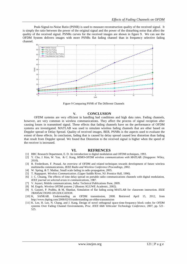
Peak-Signal-to-Noise Ratio (PSNR) is used to measure reconstruction quality of the received signal. It
is simply the ratio between the power of the original signal and the power of the disturbing noise that affect the
quality of the received signal. PSNRs curves for the received images are shown in figure 9. We can see the OFDM System delivers images with more PSNRs flat fading channel than in frequency selective fading
channel.
Figure 9 Comparing PSNR of The Different Channels
V. CONCLUSION OFDM systems are very efficient in handling bad conditions and high data rates. Fading channels,
however, are very common in wireless communications. They affect the process of signal reception after
causing losses in transmitted signal. These effects that fading channels have on the performance of OFDM
systems are investigated. MATLAB was used to simulate wireless fading channels that are ether based on
Doppler spread or Delay Spread. Quality of received images, BER, PSNRs is the aspects used to evaluate the
extent of these effects. In conclusion, fading that is caused by delay spread caused less distortion than fading
that result from Doppler spread. We found that Distortion to the received signal is higher when the speed of
the receiver is increased.
VI. REFRENCES [1] BBC Research Department, E. D. An introduction to digital modulation and OFDM techniques, 1993. [2] Y. Cho, J. Kim, W. Yan, & C. Kang, MIMO-OFDM wireless communications with MATLAB. (Singapore: Wiley,
2010).
[3] R. Frederiksen, F. Prasad, An overview of OFDM and related techniques towards development of future wireless multimedia communications, IEEE Radio and Wireless Conference Proceedings, 2002.
[4] W. Spring, & T. Mathur, Small scale fading in radio propagation, 2005. [5] T. Rappaport. Wireless Communication. (Upper Saddle River, NJ: Prentice Hall, 1996). [6] J. C. Chuang, The effects of time delay spread on portable radio communications channels with digital modulation,
IEEE journal on selected areas in communications, 1987. [7] V. Jeyasri, Mobile communications, India: Technical Publications Pune, 2009. [8] M. Engels. Wireless OFDM systems 2 (Boston: KLUWE Academic, 2002). [9] S. Gayatri, P. Prabhu, & M, Shankar, Simulation of flat fading using MATLAB for classroom instruction. IEEE
TRANSACTIONS ON EDUCATION. [10] K, SANKAR. Understanding an OFDM transmission, 2008. Retrieved April 15, 2012, from
http://www.dsplog.com/2008/02/03/understanding-an-ofdm-transmission [11] K. Lee, H. Lee, N. Chang, and J. Kang, Design of novel orthogonal space-time-frequency block codes for OFDM
systems Over Fading Channel Environments, Proc. IEEE 66th Vehicular Technology Conference, 2007, pp. 521–525.
Top Related