


Languages
Pages
Legal


Effect of Position, Usage Rate, and Per Game MinutesPlayed on NBA Player Production Curves
Garritt L. Page
Departmento de Estadística
Pontificia Universidad Católica de Chile
Bradley J. Barney
Departament of Mathematics and Statistics
Kennesaw State University
Aaron T. McGuire
Capital One
Virginia USA
Abstract
In this paper, we model a basketball player’s on-court production as a function of the per-
centiles corresponding to the number of games played. A player’s production curve is flexibly
estimated using Gaussian process regression. The hierarchical structure of the model allows
us to borrow strength across players who play the same position and have similar usage rates
and play a similar number of minutes per game. From the results of the modeling, we discuss
questions regarding the relative deterioration of production for each of the different player po-
sitions. Learning how minutes played and usage rate affect a player’s career production curve
should prove to be useful to NBA decision makers.
Key Words:Bayesian hierarchical model; Career trajectory curves; Gaussian process regres-sion
1

1 Introduction
The National Basketball Association (NBA) is a professional basketball league that is generally
considered to employ the most athletic and skilled basketball players in the world. The NBA’s
global popularity has grown rapidly, and this coupled with the uniqueness of an NBA player’s
athletic skill has resulted in increasingly large player salaries. Ideally, high producing players
would receive higher wages relative to lower producing players. However, being able to deter-
mine a player’s future production is not easy and there are numerous examples of players whose
production and compensation are misaligned. Because uncertainty surrounds future performance,
learning how different factors influence a player’s future production is of interest. In this paper we
focus on three factors: position played, minutes per game, and usage rate. That is, a player’s career
performance will be modeled as a function of time and will be grouped using the three factors
stated. We will refer to these functionals as “production curves."
Two factors that clearly influence game-by-game production are the average number of min-
utes played and usage rate. The usage rate variable is a modern basketball metric created by John
Hollinger that attempts to measure a player’s possession use per 40 minutes (?; more details are
provided in Section 2). In addition to minutes played and usage rate, it seems completely reason-
able that career production curves would depend on the position being played as each position in
the game of basketball requires a unique skill set (?) and different skills tend to deteriorate with
age at different rates.
There has been somewhat of a statistical revolution in today’s NBA decision making (?) and
a few studies have focused on career production curves. ? studied career trends of basketball
players in the Turkish Basketball League. In other sports, ? used a Bayesian hierarchical model to
compare career production of baseball players, hockey players and golfers regardless of era played.
? compared the careers of pitchers in major league baseball. A connected avenue of research is
that of investigating how aging impacts performance. For example, ? and ? estimated the age that
2

corresponds to an NBA player’s peak performance.
In this paper we employ a hierarchical Bayes model to estimate not only individual player
production curves but also the process that generates the individual curves according to position,
usage rate, and minutes played per game. The observation and process levels of the hierarchy
are modeled using Gaussian process (GP) regressions (see ? for GPs and ? for hierarchical GP
modeling). Therefore, individual player curves as well as the position by usage rate by minutes
per game (hereafter p×u×m) mean curves are modeled very flexibly. Using a hierarchical model
allows us to borrow strength across individuals that belong to the same p× u×m category when
estimating process level production curves. Unlike other studies about NBA aging, we are not
necessarily interested in estimating a player’s “prime" (though this is readily available from this
methodology); rather principal interest lies in estimating the entire career production curve.
The remainder of this article is organized as follows. Section 2 contains a description of the
data and Section 3 describes the Gaussian process hierarchical regression model employed. Section
4 outlines the results of the study and Section 5 provides a brief discussion.
2 Description of Data
Game-by-game summaries (including playoffs) for each retired player drafted in the 1992-1997
NBA drafts and who participated in at least 100 games were collected (which provided a pool of
178 players). The 100 game minimum was instituted to help us enact our binning method which
was implemented for computation and interpretation purposes. (This also reduces the noise intro-
duced by the careers of players that contain little information regarding the processes of interest.)
The game-by-game summaries collected include typical box-score metrics in addition to a few
“modern" basketball metrics. Among these we selected John Hollinger’s so called Game Score (?)
as a response variable (more details are provided in the subsequent paragraph). For an aging met-
ric (and as the independent variable) we use percentiles associated with number of games played.
3
Other aging metrics such as player age could have been considered but we feel using games played
better represents the stresses that game action applies to the body. Additionally, it allowed us to
bin the process in a way that made comparisons and borrowing of strength among and between
groups reasonable.
It is fairly well known that a gold standard “production” metric in basketball doesn’t exist (?).
All metrics–from win shares (?) to value over replacement player (VORP)–provide an incom-
plete picture of a player’s worth. With that in mind, we somewhat arbitrarily chose to use John
Hollinger’s Game Score to represent player game production. Game Score is the following linear
combination of common box-score summaries:
GmSc =PT S+ .4FG− .7FGA− .4FT M+ .7ORB+ .3DRB+ST L+ .7AST+
.7BLK− .4PF−TOV, (1)
where PTS denotes total number of points scored in a game, FG denotes the number of field goals
made, FGA the number of field goals attempted, FTM the number of free throws made, ORB the
number of offensive rebounds, DRB the number of defensive rebounds, STL the number of steals,
AST the number of assists, BLK the number of blocks, PF the number of personal fouls, and TOV
the number of turn-overs. This statistic is a well known “add the good, subtract the bad” game-
by-game production metric that provides a fairly decent evaluation of a player’s production during
any given game. That said, it has been criticized for overvaluing points scored by poor shooters
(?), for undervaluing defensive contributions, and for ignoring quality of opponent.
As mentioned in the introduction, for player-specific covariates we used position, usage rate,
and average minutes per game. These three variables seem to partition players reasonably well
with regards to Game Score making it sensible to borrow strength among the subgroups. Usage
4

rate is defined as follows:
Usage Rate =[FGA+(FTA×0.44)+(AST ×0.33)+TOV ]×40×League Pace
(Minutes × Team Pace), (2)
(?, p. 5), with Team Pace defined as
Team Pace =[FGA−ORB+TOV +(FTA×0.44)]×48
(Team Minutes × 2)(3)
and League Pace defined as the average Team Pace for all NBA teams (p. 1). (In defining Team
Pace, all quantities inside the brackets represent combined totals–for the team and its opponents–in
games played by the team that season.) We categorized each player’s usage rate as being high usage
or low usage by comparing the player’s average usage rate (across all games) to the corresponding
median value among all players considered. We likewise categorized each player’s minutes played
per game as being either high or low via a comparison to the median value. Thus, a player was
categorized as high usage high minute, high usage low minute, low usage high minute, or low usage
low minute. Although a player’s usage rate and minutes played per game might have changed
substantially throughout his career, our method of categorization did not permit the player’s group
membership to change.
With regards to position, we used a trichotomous categorization. Although there are five des-
ignated positions in a basketball game – two guards (a point guard and a shooting guard), two
forwards (a small forward and a power forward), and a center, there is some overlap between the
five positions. Many players are, for instance, a guard-forward or a forward-center. Ambiguity in
using five positions to classify players arises because many shooting guards and small forwards
are indistinguishable depending on their team’s lineup decisions. Likewise, centers may play the
power forward position depending on an opponent’s skill set. Therefore, as is typically currently
done, we categorize players as point guards, “wings”, and “bigs”. In basketball terms, a “wing”
is essentially a guard-forward – “wing” can be used to describe large shooting guards and small
5

forwards. By characterizing centers and power forwards together as “bigs,” we can lessen the com-
mon problem of classifying players of extremely ambiguous position. The number of players in
each of the 12 groups is provided in Table 1
Usage/Minutes Bigs Wings Point Guards Total
U+/M+ 13 17 6 36U+/M- 13 20 6 39U-/M+ 4 8 3 15U-/M- 36 26 16 78Total 31 71 56 178
Table 1: Number of players in each of the j = 1, . . . ,12 p×u×m groups
We borrow strength between players by considering 12 different groups, corresponding to the
12 possible p×u×m combinations. Being able to borrow strength between players (and ultimately
make comparisons) requires in some sense a matching of career trajectories as players have played
a varying numbers of games and minutes. This is of course no easy task. The ideal situation would
be for the explanatory variable for each player to more or less represent the same time frame.
We believe that one way this can be accomplished is to match the percentiles associated with the
number of games played for each player. This naturally leads to considering 100 bins. We use zit
to denote the games comprising the tth percentile among all games played by player i. We will use
yit to denote the mean Game Score for player i computed across all games in zit . In what follows
we will refer to zit as “game percentile.” We employ this binning process with the understanding
that some players have longer careers than others, so the last percentile for one player might be
during his second season while for another player it might be during his fifteenth season. However,
we do feel that using usage rate and minutes played to group players does a good job of mitigating
this possibility and thus grouped player career trajectories match fairly well (making borrowing of
strength sensible).
6

0 20 40 60 80 100
05
1015
2025
Glenn Robinson
Game Percentile
Gam
e S
core
0 20 40 60 80 100
05
1015
2025
Shaquille ONeal
Game Percentile
Gam
e S
core
0 20 40 60 80 100
05
1015
2025
Brevin Knight
Game Percentile
Gam
e S
core
Figure 1: Plots of Hollinger’s Game Score statistic versus game percentile for Glenn Robinson,Shaquille O’neal, and Brevin Knight
3 Model
It is reasonable to believe that a player’s career Game Score curve as a function of game percentile
is not linear. Some player career production curves display an initial increasing trend until a plateau
where the player is most productive, eventually followed by a decreasing trend towards the end
of the career. This indeed seems to be the case for Glenn Robinson (See Figure 1). However,
Shaquille O’Neal displays a brief dip early in his peak period and a relatively long period of
decline, while Brevin Knight oscillates between increasing and decreasing production. Thus, it
appears as if production curves are highly variable from one player to the next. We anticipate there
might be dramatic differences between players based on position, minutes played, and usage rate,
and we therefore allow for 12 different group-mean curves, one for each p×u×m group. But we
also recognize that even players in the same group might exhibit vastly different production curves.
In light of this, production curves should be modeled flexibly along with the curves associated with
the 12 p× u×m groups. This can be handled via a hierarchical model where GP regression is
employed both at the observation level and process level of the hierarchy. As GPs are central to
our modeling approach, they are briefly introduced in the next subsection.
7

3.1 Gaussian Process
We very briefly introduce Gaussian processes (GP) here. For a more general and thorough intro-
duction see ?. (In what follows all letters in bold font will denote vectors.) Generally speaking,
a GP can be considered as a distribution over functions f (z) : ℜ→ ℜ where any finite number
of realizations ( f (z1), f (z2), . . . , f (zT )) follow a multivariate Gaussian distribution that is com-
pletely characterized by a mean function m(z) : ℜT → ℜT and positive definite covariance func-
tion K(z;θ) : ℜT →ℜT×T . Here, θ is a vector of parameters and z = (z1, . . . ,zT ). Thus, if we let
f denote some unknown function with independent variables z1, . . . ,zT , then f follows a GP (com-
monly denoted as f ∼ G P(m(z),K(z;θ))) if for any T < ∞ the realizations of f are distributed
as
[ f (z1), f (z2), . . . , f (zT )]′ ∼ NT (m(z),K(z;θ)).
What is of principal interest in the current modeling is the estimation of mean function m(z) while
f is secondary. We make these ideas more concrete relative to the NBA production curve context
in the next section.
Selecting an appropriate covariance function can be a difficult model selection exercise when
using GPs. For computational convenience and sake of simplicity, we employ the commonly used
Gaussian covariance function. The covariance matrix produced by this function has (i, `) element
given by the following form
φ exp{−ρ (zi− z`)
2}, (4)
where ρ is a correlation scale parameter that controls how much the functional curve is allowed
to vary across time (as ρ ↑ the curve becomes more linear), and φ is a variance parameter that
controls the smoothness of the curve (as φ ↑ the curve becomes more up and down). Thus for this
covariance function θ = (ρ,φ).
8

3.2 Hierarchical specification of the model
As stated earlier, we use zit to denote the games in the ith player’s tth career length percentile,
t = 1, . . . ,100. Since the entries of zi = (zi1, . . . ,zi100) are equal for each player, for notational
convenience in what follows we use z to denote each players game percentile vector. Also, we
use yit to denote the ith player’s average production during games in zit . We use xi to denote a
player-specific variable indicating to which of the j = 1, . . . ,12 p×u×m groups player i belongs.
Each player’s Game Score is then modeled as a function of game percentile as follows
yit = β0i + fi(zt)+ εit with εitind∼ N(0,σ2
i ). (5)
Recognizing that inevitably some players are more productive than others, we include a player
specific “intercept” β0i to red account for some of the systematic variability in average player
performance over time. To equation (5) we add the following hierarchical structure
fi(z)|xi = j ∼ G P(m j(z),K j(z;φ j,ρ j)), (6)
m j(z)∼ G P(0,K(z;s,r)), (7)
where m j(z) and K(z;φ j,ρ j) denote the jth red group’s mean and covariance functions with s and
r being user supplied. We are now modeling each player’s production curve and the mean curve for
each of the j = 1, . . . ,12 p×u×m groups using GP regressions. This allows us to estimate group
curves while borrowing strength across players that we expect to have somewhat similar produc-
tion curves. To make the MCMC algorithm employed (details of which are in the next section)
numerically stable, we standardized z to the unit interval by dividing each entry of z by 100. We
note that this does not affect the shape of the mean curve, so we use the original units in z when
interpreting the results. To complete the Bayesian model we assigned fairly diffuse (Ga(1,1)) in-
dependent priors for φ= (φ1, . . . ,φ12) and ρ= (ρ1, . . . ,ρ12), a diffuse Gaussian prior (N(0,100))
9
for β0i and set s = 100 and r = 1 which provides prior covariance matrices with variances equal to
100.
A few comments of the features that accompany this model are warranted. The methodology is
extremely flexible in estimating production curves. No rigid polynomial forms have been assumed.
The uncertainty of production curve form has been incorporated in all parameter estimates. Also,
a natural mechanism of Bayesian hierarchical modeling is that the estimates for individuals are
shrunk to the overall mean.
3.3 Computation
The joint posterior distributions arrived at through GP regression are intractable analytically. Be-
cause exact sampling is not possible, we resort to MCMC methods to sample from the joint poste-
rior distribution. Specifically, we use a hybrid Gibbs sampler (?) and Metropolis-Hastings (M-H)
algorithm (? and ?). Gibbs steps can be used to update the f (·)i’s, the m(·) j’s, and the β0i’s. To
update φ and ρ a random walk M-H step with Gaussian proposal distributions was used. Conver-
gence was assessed using history plots of 3000 MCMC draws. These were collected by running
three independent chains until 1000 MCMC iterates were obtained after a burn-in of 10,000 and a
thinning of 50.
4 Results
Results are presented graphically. We briefly highlight fitted curves for individual players and
variability among the β0i’s, but focus the majority of our attention on the estimates of the 12
m j(·)’s. As a means of shedding some light on the variability of the β0i’s we calculated the standard
deviation of the 178 β0i posterior means. This standard deviation is only 1.57. Thus the β0i’s do
not capture much of the player-to-player variability.
10

0 20 40 60 80 100
05
1015
2025
Glenn Robinson
Game Percentile
Gam
e S
core
0 20 40 60 80 100
05
1015
2025
Shaquille ONeal
Game Percentile
Gam
e S
core
0 20 40 60 80 100
05
1015
2025
Brevin Knight
Game Percentile
Gam
e S
core
Figure 2: Individual fitted curves and 95% mean curve credible intervals for Game Score corre-sponding to Glenn Robinson, Shaquille O’neal, and Brevin Knight.
4.1 Estimated Curves for Individual Players
As a means to show individual estimated curves are reasonable, Figure 2 provides fitted curves
with 95% credible bands corresponding to the three players highlighted in Figure 1 (note that zt
were transformed to their original units). The fits are all quite sensible.
4.2 Average Group Production Curves and Comparisons
Figure 3 displays the mean curves and error bands for each of the 12 p× u×m categories for
Game Score. Notice that the red uncertainty associated with production curves is not the same
across groups; the red uncertainty is especially large for point guards and for players with high
minutes but low usage rates. This is to be expected as the number of players in each group varies.
Figure 4 depicts the same process level production curves as Figure 3, but including the 12
curves in the same plot aids in comparison across groups. It appears that players with high minutes
per game tend to experience more dramatic changes over the course of their careers than players
with low minutes. This is particularly apparent for players who, in addition to high minutes, have
high usage rates. There is also some indication that players with high minutes and high usage rates
tend to reach their peak earlier. One possible explanation is that they more rapidly accumulate
11

Game Percentile
Gam
e S
core
-5
0
5
10
15
20
0 20 40 60 80 100
big
U-/M-
wing
U-/M-
0 20 40 60 80 100
pg
U-/M-
big
U-/M+
wing
U-/M+
-5
0
5
10
15
20pg
U-/M+
-5
0
5
10
15
20big
U+/M-
wingU+/M-
pg
U+/M-
big
U+/M+
0 20 40 60 80 100
wing
U+/M+
-5
0
5
10
15
20
pg
U+/M+
Figure 3: Process level mean production curves with 95% posterior credible bands correspondingto Game Score for each of the 12 p×u×m categories. In the row labels, the first symbol depictsusage rate (+ for high, − for low), and the second depicts minutes per game.
12

wear and tear on their bodies with each game because of the time and energy exerted. Though not
as pronounced, there also appears to be a tendency for bigs to peak slightly earlier than wings and
point guards, and for point guards to peak slightly later than the others.
Table 2 provides an estimated mean game percentile for which the maximum game score is
achieved. As indicated by Figure (4) the point guard position generally tends to attain peak per-
formance around the 50th percentile, while for wings this occurs around the 45th and for bigs
it is around the 40th. That said, the variability is quite large in a few categories and therefore
conclusions must be drawn cautiously.
Usage/Minutes Bigs Wings Point Guards
U+/M+ 36.0 (3.5) 42.7 (3.9) 43.2 (4.7)U+/M- 38.6 (5.1) 47.4 (4.5) 42.2 (19.7)U-/M+ 36.6 (12.4) 41.1 (5.4) 52.2 (10.8)U-/M- 41.1 (4.2) 44.7 (7.1) 50.0 (7.5)
Table 2: Estimated mean (sd) game percentile where maximum Game Score is achieved for j =1, . . . ,12 p×u×m groups
Figure 5 displays the individual production curves for the six high usage, high minutes point
guards included in our analyses. It can be seen that there is some variation in the overall curve
heights, yet there is a tendency for these players to have a gradual increase followed by a rapid
decline. This overall tendency supports our choice of categories because, imperfect as the choice
may be, the individual curves have fairly similar heights and shapes.
5 Conclusions
We have posed a hierarchical GP regression model that flexibly estimates career production curves
for 12 p× u×m categories. The general red finding from this is that aging trends do impact
natural talent evaluation of NBA players. Point guards appear to exhibit a different aging pattern
than wings or bigs when it comes to Hollinger’s Game Score, with a slightly later peak and a much
13

0 20 40 60 80 100
05
1015
Game Percentile
Gam
e S
core
U+/M+ pgU+/M+ wingU+/M+ big
U+/M- pgU+/M- wingU+/M- big
U-/M+ pgU-/M+ wingU-/M+ big
U-/M- pgU-/M- wingU-/M- big
Figure 4: Process level mean production curves corresponding to game score for each of the 12p×u×m categories. In the legend, the first symbol depicts usage rate (+ for high,− for low), andthe second depicts minutes per game.
14

0 20 40 60 80 100
05
1015
20
PG high usage high minutes
Game Percentile
Reb
ound
Per
cent
age
Sam CassellAnfernee HardawayAllen IversonStephon Marbury
Damon StoudamireNick Van ExelGroup Mean
Figure 5: Individual mean player production curves for the six high usage, high minutes pointguards. The solid line depicts the group average.
15

steeper decline once that peak is met. The fact that the average point guard spends more of his
career improving his game score is not lost on talent evaluators in the NBA, and as such, point
guards are given more time on average to perform the functions of a rotation player in the NBA.
Also, regardless of position, players with high minutes tend to have greater fluctuation in Game
Score production over time. While these are the general results of interest, the difference between
individual curves is also of note.
The information gained from this modeling exercise is a nice starting point in the study of NBA
player production curves. Obviously production curves are functions of much more than the three
covariates that we considered. Factors such as quality of teammates, coaching philosophy and
injury surely influence production (?). Including these variables as they become available could
potentially improve inference. Additionally, future research could focus on estimating career red
timepoints that correspond to slope inflections of a production curve in addition to incorporating a
“team role” variable. For NBA decision-makers mulling over new contracts, research of this nature
could be very valuable in determining contracts on-the-margins, and is without question a worthy
subject of future study.
Appendices
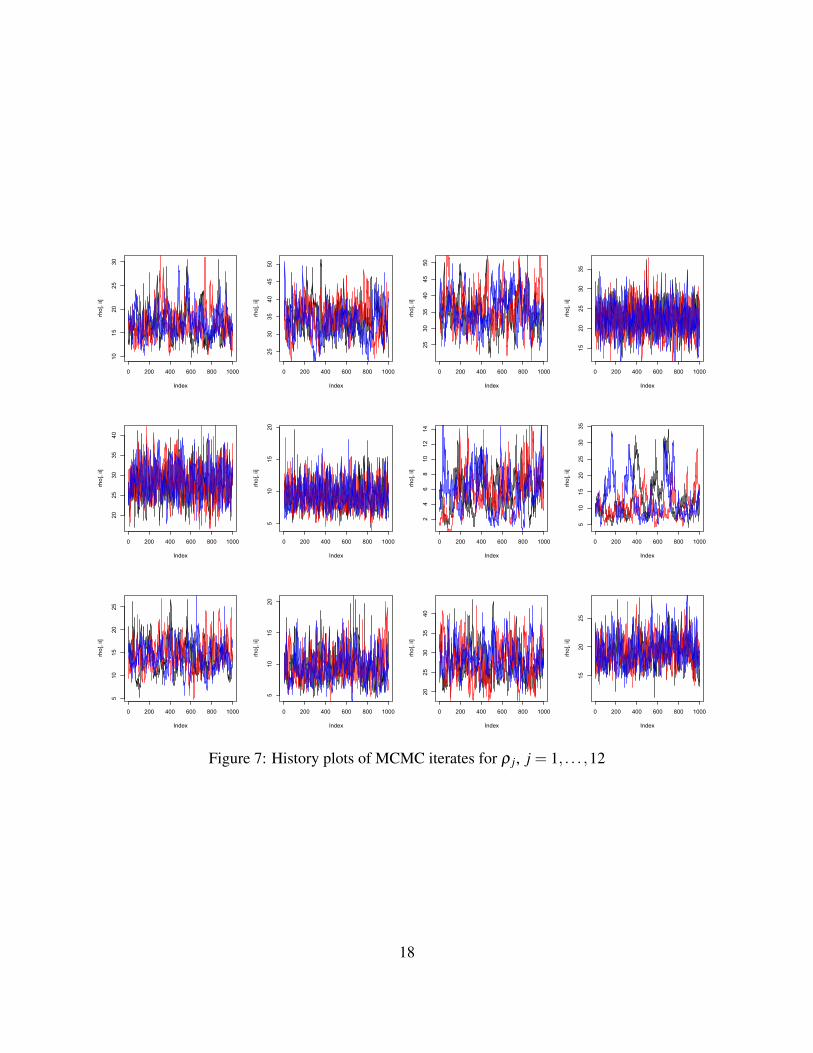
A MCMC iterate history plots
We provide a few arbitrarily selected history plots of MCMC iterates. The first set corresponds
to the first entry of µ(·) j for the twelve groups, and the second set corresponds to ρ j for the
twelve groups. The general indication these plots provide is that the MC chains have reached their
equilibrium states.
16

0 200 400 600 800 1000
-20
24
68
Index
mu[
1, ii
, ]
0 200 400 600 800 1000
-20
24
68
Index
mu[
1, ii
, ]
0 200 400 600 800 1000
24
68
10
Index
mu[
1, ii
, ]
0 200 400 600 800 1000
-10
-50
510
15
Index
mu[
1, ii
, ]
0 200 400 600 800 1000
-50
510
15
Index
mu[
1, ii
, ]
0 200 400 600 800 1000
05
1015
Index
mu[
1, ii
, ]
0 200 400 600 800 1000
-50
510
15
Index
mu[
1, ii
, ]
0 200 400 600 800 1000
-4-2
02
46
8
Index
mu[
1, ii
, ]
0 200 400 600 800 1000
02
46
810
Index
mu[
1, ii
, ]
0 200 400 600 800 1000
05
1015
20
Index
mu[
1, ii
, ]
0 200 400 600 800 1000
24
68
1012
Index
mu[
1, ii
, ]
0 200 400 600 800 1000
46
810
1214
16
Index
mu[
1, ii
, ]
Figure 6: History plots of MCMC iterates for the first entry of µ(·) j, j = 1, . . . ,12
17
0 200 400 600 800 1000
1015
2025
30
Index
rho[
, ii]
0 200 400 600 800 1000
2530
3540
4550
Index
rho[
, ii]
0 200 400 600 800 1000
2530
3540
4550
Index
rho[
, ii]
0 200 400 600 800 1000
1520
2530
35
Index
rho[
, ii]
0 200 400 600 800 1000
2025
3035
40
Index
rho[
, ii]
0 200 400 600 800 1000
510
1520
Index
rho[
, ii]
0 200 400 600 800 1000
24
68
1012
14
Index
rho[
, ii]
0 200 400 600 800 1000
510
1520
2530
35
Index
rho[
, ii]
0 200 400 600 800 1000
510
1520
25
Index
rho[
, ii]
0 200 400 600 800 1000
510
1520
Index
rho[
, ii]
0 200 400 600 800 1000
2025
3035
40
Index
rho[
, ii]
0 200 400 600 800 1000
1520
25
Index
rho[
, ii]
Figure 7: History plots of MCMC iterates for ρ j, j = 1, . . . ,12
18
Top Related