


Languages
Pages
Legal


Econometric Analysis of Financial Market Data1
ZONGWU CAI
E-mail address: [email protected]
Department of Mathematics & Statistics and Department of Economics,
University of North Carolina, Charlotte, NC 28223, U.S.A.
Wang Yanan Institute for Studies in Economics, Xiamen University, China
February 3, 2010
c©2010, ALL RIGHTS RESERVED by ZONGWU CAI
1This manuscript may be printed and reproduced for individual or instructional use, but maynot be printed for commercial purposes.

i
Preface
The main purpose of this lecture notes is to provide you with a foundation to pursue thebasic theory and methodology as well as applied projects involving the skills to analyzingfinancial data. This course also gives an overview of the econometric methods (models andtheir modeling techniques) applicable to financial economic modeling. More importantly, itis the ultimate goal of bringing you to the research frontier of the empirical (quantitative)finance. To model financial data, some packages will be used such as R, which is a veryconvenient programming language for doing homework assignments and projects. You candownload it for free from the web site at http://www.r-project.org/.
Several projects, including the heavy computer works, are assigned throughout the semester.The group discussion is allowed to do the projects and the computer related homework, par-ticularly writing the computer codes. But, writing the final report to each project or homeassignment must be in your own language. Copying each other will be regarded as a cheating.If you use the R language, similar to SPLUS, you can download it from the public web siteat http://www.r-project.org/ and install it into your own computer or you can use PCs atour labs. You are STRONGLY encouraged to use (but not limited to) the package R sinceit is a very convenient programming language for doing statistical analysis and Monte Carolsimulations as well as various applications in quantitative economics and finance. Of course,you are welcome to use any one of other packages such as SAS, MATLAB, GAUSS, andSTATA. But, I might not have an ability of giving you a help if doing so.
How to Install R ?
The main package used is R, which is free from R-Project for Statistical Computing.
(1) go to the web site http://www.r-project.org/;
(2) click CRAN;
(3) choose a site for downloading, say http://cran.cnr.Berkeley.edu;
(4) click Windows (95 and later);
(5) click base;
(6) click R-2.10.1-win32.exe (Version of December 14, 2009) to save this file first andthen run it to install (Note that the setup program is 32 megabytes and it is updatedalmost every three months).
The above steps install the basic R into your computer. If you need to install otherpackages, you need to do the followings:
(7) After it is installed, there is an icon on the screen. Click the icon to get into R;
(8) Go to the top and find packages and then click it;

ii
(9) Go down to Install package(s)... and click it;
(10) There is a new window. Choose a location to download packages, say USA(CA1),move mouse to there and click OK;
(11) There is a new window listing all packages. You can select any one of packages andclick OK, or you can select all of them and then click OK.
Data Analysis and Graphics Using R – An Introduction (109 pages)
I encourage you to download the file r-notes.pdf (109 pages) which can be downloadedfrom http://www.math.uncc.edu/˜ zcai/r-notes.pdf and learn it by yourself. Pleasesee me if any questions.
CRAN Task View: Empirical Finance
This CRAN Task View contains a list of packages useful for empirical work in Finance andit can be downloaded from the web site athttp://cran.cnr.berkeley.edu/src/contrib/Views/Finance.html.
CRAN Task View: Computational Econometrics
Base R ships with a lot of functionality useful for computational econometrics, in particularin the stats package. This functionality is complemented by many packages on CRAN. Itcan be downloaded from the web site athttp://cran.cnr.berkeley.edu/src/contrib/Views/Econometrics.html.
Contents
1 A Motivation Example 11.1 Introduction . . . . . . . . . . . . . . . . . . . . . . . . . . . . . . . . . . . . 11.2 Preliminary Statistical Analysis . . . . . . . . . . . . . . . . . . . . . . . . . 21.3 Jump-Diffusion Modeling Procedures . . . . . . . . . . . . . . . . . . . . . . 61.4 Pricing American-style Options Using Stratification Simulation Method . . . 81.5 Hedging Issues . . . . . . . . . . . . . . . . . . . . . . . . . . . . . . . . . . 101.6 Conclusions . . . . . . . . . . . . . . . . . . . . . . . . . . . . . . . . . . . . 111.7 References . . . . . . . . . . . . . . . . . . . . . . . . . . . . . . . . . . . . . 11
2 Basic Concepts of Prices and Returns 132.1 Introduction . . . . . . . . . . . . . . . . . . . . . . . . . . . . . . . . . . . . 132.2 Basic Definitions . . . . . . . . . . . . . . . . . . . . . . . . . . . . . . . . . 14
2.2.1 Time Value of Money . . . . . . . . . . . . . . . . . . . . . . . . . . . 142.2.2 Assets and Markets . . . . . . . . . . . . . . . . . . . . . . . . . . . . 152.2.3 Financial Theory . . . . . . . . . . . . . . . . . . . . . . . . . . . . . 16
2.3 Statistical Features . . . . . . . . . . . . . . . . . . . . . . . . . . . . . . . . 172.3.1 Prices . . . . . . . . . . . . . . . . . . . . . . . . . . . . . . . . . . . 172.3.2 Frequency of Observations . . . . . . . . . . . . . . . . . . . . . . . . 172.3.3 Definition of Returns . . . . . . . . . . . . . . . . . . . . . . . . . . . 17
2.4 Stylized Facts for Financial Returns . . . . . . . . . . . . . . . . . . . . . . . 212.5 Problems . . . . . . . . . . . . . . . . . . . . . . . . . . . . . . . . . . . . . . 262.6 References . . . . . . . . . . . . . . . . . . . . . . . . . . . . . . . . . . . . . 30
3 Linear Time Series Models and Their Applications 313.1 Stationary Stochastic Process . . . . . . . . . . . . . . . . . . . . . . . . . . 323.2 Constant Expected Return Model . . . . . . . . . . . . . . . . . . . . . . . . 34
3.2.1 Model Assumptions . . . . . . . . . . . . . . . . . . . . . . . . . . . . 343.2.2 Regression Model Representation . . . . . . . . . . . . . . . . . . . . 343.2.3 CER Model of Asset Returns and Random Walk Model of Asset Prices 353.2.4 Monte Carlo Simulation Method . . . . . . . . . . . . . . . . . . . . . 363.2.5 Estimation . . . . . . . . . . . . . . . . . . . . . . . . . . . . . . . . . 363.2.6 Statistical Properties of Estimates . . . . . . . . . . . . . . . . . . . . 38
3.3 AR(1) Model . . . . . . . . . . . . . . . . . . . . . . . . . . . . . . . . . . . 383.3.1 Estimation and Tests . . . . . . . . . . . . . . . . . . . . . . . . . . . 403.3.2 White Noise Hypothesis . . . . . . . . . . . . . . . . . . . . . . . . . 41
iii
CONTENTS iv
3.3.3 Unit Root . . . . . . . . . . . . . . . . . . . . . . . . . . . . . . . . . 413.3.4 Estimation and Tests in the Presence of a Unit Root . . . . . . . . . 42
3.4 MA(1) Model . . . . . . . . . . . . . . . . . . . . . . . . . . . . . . . . . . . 453.5 ARMA, ARIMA, and ARFIMA Processes . . . . . . . . . . . . . . . . . . . 45
3.5.1 ARMA(1,1) Process . . . . . . . . . . . . . . . . . . . . . . . . . . . 453.5.2 ARMA(p,q) Process . . . . . . . . . . . . . . . . . . . . . . . . . . . 463.5.3 AR(p) Model . . . . . . . . . . . . . . . . . . . . . . . . . . . . . . . 483.5.4 MA(q) . . . . . . . . . . . . . . . . . . . . . . . . . . . . . . . . . . . 503.5.5 AR(∞) Process . . . . . . . . . . . . . . . . . . . . . . . . . . . . . . 523.5.6 MA(∞) Process . . . . . . . . . . . . . . . . . . . . . . . . . . . . . . 523.5.7 ARIMA Processes . . . . . . . . . . . . . . . . . . . . . . . . . . . . . 523.5.8 ARFIMA Process . . . . . . . . . . . . . . . . . . . . . . . . . . . . . 52
3.6 R Commands . . . . . . . . . . . . . . . . . . . . . . . . . . . . . . . . . . . 563.7 Regression Models With Correlated Errors . . . . . . . . . . . . . . . . . . . 563.8 Comments on Nonlinear Models and Their Applications . . . . . . . . . . . . 563.9 Problems . . . . . . . . . . . . . . . . . . . . . . . . . . . . . . . . . . . . . . 57
3.9.1 Problems . . . . . . . . . . . . . . . . . . . . . . . . . . . . . . . . . 573.9.2 R Code . . . . . . . . . . . . . . . . . . . . . . . . . . . . . . . . . . 60
3.10 Appendix A: Linear Forecasting . . . . . . . . . . . . . . . . . . . . . . . . . 613.11 Appendix B: Forecasting Based on AR(p) Model . . . . . . . . . . . . . . . . 623.12 Appendix C: Random Variables . . . . . . . . . . . . . . . . . . . . . . . . . 643.13 References . . . . . . . . . . . . . . . . . . . . . . . . . . . . . . . . . . . . . 67
4 Predictability of Asset Returns 694.1 Introduction . . . . . . . . . . . . . . . . . . . . . . . . . . . . . . . . . . . . 69
4.1.1 Martingale Hypothesis . . . . . . . . . . . . . . . . . . . . . . . . 694.1.2 Tests of MD . . . . . . . . . . . . . . . . . . . . . . . . . . . . . . . . 70
4.2 Random Walk Hypotheses . . . . . . . . . . . . . . . . . . . . . . . . . . . . 714.2.1 IID Increments (RW1) . . . . . . . . . . . . . . . . . . . . . . . . . . 714.2.2 Independent Increments (RW2) . . . . . . . . . . . . . . . . . . . . . 714.2.3 Uncorrelated Increments (RW3) . . . . . . . . . . . . . . . . . . . . . 724.2.4 Unconditional Mean is the Best Predictor (RW4) . . . . . . . . . . . 72
4.3 Tests of Predictability . . . . . . . . . . . . . . . . . . . . . . . . . . . . . . 724.3.1 Nonparametric Tests . . . . . . . . . . . . . . . . . . . . . . . . . . . 734.3.2 Autocorrelation Tests . . . . . . . . . . . . . . . . . . . . . . . . . . . 764.3.3 Variance Ratio Tests . . . . . . . . . . . . . . . . . . . . . . . . . . . 774.3.4 Trading Rules and Market Efficiency . . . . . . . . . . . . . . . . . . 80
4.4 Empirical Results . . . . . . . . . . . . . . . . . . . . . . . . . . . . . . . . . 844.4.1 Evidence About Returns Predictability Using VR and Autocorrelation Tests 844.4.2 Cross Lag Autocorrelations and Lead-Lag Relations . . . . . . . . . . 854.4.3 Evidence About Returns Predictability Using Trading Rules . . . . . 86
4.5 Predictability of Real Stock and Bond Returns . . . . . . . . . . . . . . . . . 874.5.1 Financial Predictors . . . . . . . . . . . . . . . . . . . . . . . . . . . 874.5.2 Models and Modeling Methods . . . . . . . . . . . . . . . . . . . . . 88
4.6 A Recent Perspective on Predictability of Asset Return . . . . . . . . . . . . 95
CONTENTS v
4.6.1 Introduction . . . . . . . . . . . . . . . . . . . . . . . . . . . . . . . . 964.6.2 Conditional Means . . . . . . . . . . . . . . . . . . . . . . . . . . . . 964.6.3 Conditional Variances . . . . . . . . . . . . . . . . . . . . . . . . . . 984.6.4 Distributions . . . . . . . . . . . . . . . . . . . . . . . . . . . . . . . 984.6.5 The future . . . . . . . . . . . . . . . . . . . . . . . . . . . . . . . . . 99
4.7 Comments on Predictability Based on Nonlinear Models . . . . . . . . . . . 1014.8 Problems . . . . . . . . . . . . . . . . . . . . . . . . . . . . . . . . . . . . . . 101
4.8.1 Exercises for Homework . . . . . . . . . . . . . . . . . . . . . . . . . 1014.8.2 R Codes . . . . . . . . . . . . . . . . . . . . . . . . . . . . . . . . . . 1024.8.3 Project #1 . . . . . . . . . . . . . . . . . . . . . . . . . . . . . . . . 103
4.9 References . . . . . . . . . . . . . . . . . . . . . . . . . . . . . . . . . . . . . 104
5 Market Model 1115.1 Introduction . . . . . . . . . . . . . . . . . . . . . . . . . . . . . . . . . . . . 1115.2 Assumptions About Asset Returns . . . . . . . . . . . . . . . . . . . . . . . 1125.3 Unconditional Properties of Returns . . . . . . . . . . . . . . . . . . . . . . . 1125.4 Conditional Properties of Returns . . . . . . . . . . . . . . . . . . . . . . . . 1135.5 Beta as a Measure of Portfolio Risk . . . . . . . . . . . . . . . . . . . . . . . 1145.6 Diagnostics for Constant Parameters . . . . . . . . . . . . . . . . . . . . . . 1155.7 Estimation and Hypothesis Testing . . . . . . . . . . . . . . . . . . . . . . . 1165.8 Problems . . . . . . . . . . . . . . . . . . . . . . . . . . . . . . . . . . . . . . 1165.9 References . . . . . . . . . . . . . . . . . . . . . . . . . . . . . . . . . . . . . 117
6 Event-Study Analysis 1196.1 Introduction . . . . . . . . . . . . . . . . . . . . . . . . . . . . . . . . . . . . 1196.2 Outline of an Event Study . . . . . . . . . . . . . . . . . . . . . . . . . . . . 1206.3 Models for Measuring Normal Returns . . . . . . . . . . . . . . . . . . . . . 1216.4 Measuring and Analyzing Abnormal Returns . . . . . . . . . . . . . . . . . . 122
6.4.1 Estimation Procedure . . . . . . . . . . . . . . . . . . . . . . . . . . 1236.4.2 Aggregation of Abnormal Returns . . . . . . . . . . . . . . . . . . . . 1246.4.3 Modifying the Null Hypothesis: . . . . . . . . . . . . . . . . . . . . . 1276.4.4 Nonparametric Tests . . . . . . . . . . . . . . . . . . . . . . . . . . . 1276.4.5 Cross-Sectional Models . . . . . . . . . . . . . . . . . . . . . . . . . . 1296.4.6 Power of Tests . . . . . . . . . . . . . . . . . . . . . . . . . . . . . . . 131
6.5 Further Issues . . . . . . . . . . . . . . . . . . . . . . . . . . . . . . . . . . . 1326.6 Problems . . . . . . . . . . . . . . . . . . . . . . . . . . . . . . . . . . . . . . 1346.7 References . . . . . . . . . . . . . . . . . . . . . . . . . . . . . . . . . . . . . 135
7 Introduction to Portfolio Theory 1367.1 Introduction . . . . . . . . . . . . . . . . . . . . . . . . . . . . . . . . . . . . 136
7.1.1 Efficient Portfolios With Two Risky Assets . . . . . . . . . . . . . . . 1377.1.2 Efficient Portfolios with One Risky Asset and One Risk-Free Asset . . 1387.1.3 Efficient portfolios with two risky assets and a risk-free asset . . . . . 139
7.2 Efficient Portfolios with N risky assets . . . . . . . . . . . . . . . . . . . . . 1407.3 Another Look at Mean-Variance Efficiency . . . . . . . . . . . . . . . . . . . 142
CONTENTS vi
7.4 The Black-Litterman Model . . . . . . . . . . . . . . . . . . . . . . . . . . . 1447.4.1 Expected Returns . . . . . . . . . . . . . . . . . . . . . . . . . . . . . 1447.4.2 The Black-Litterman Model . . . . . . . . . . . . . . . . . . . . . . . 1457.4.3 Building the Inputs . . . . . . . . . . . . . . . . . . . . . . . . . . . . 147
7.5 Estimation of Covariance Matrix . . . . . . . . . . . . . . . . . . . . . . . . 1477.5.1 Estimation Approaches . . . . . . . . . . . . . . . . . . . . . . . . . . 1487.5.2 Shrinkage estimator of the covariance matrix . . . . . . . . . . . . . . 1507.5.3 Recent Developments . . . . . . . . . . . . . . . . . . . . . . . . . . . 152
7.6 Problems . . . . . . . . . . . . . . . . . . . . . . . . . . . . . . . . . . . . . . 1527.7 References . . . . . . . . . . . . . . . . . . . . . . . . . . . . . . . . . . . . . 153
8 Capital Asset Pricing Model 1558.1 Review of the CAPM . . . . . . . . . . . . . . . . . . . . . . . . . . . . . . . 1558.2 Statistical Framework for Estimation and Testing . . . . . . . . . . . . . . . 157
8.2.1 Time-Series Regression . . . . . . . . . . . . . . . . . . . . . . . . . . 1588.2.2 Cross-Sectional Regression . . . . . . . . . . . . . . . . . . . . . . . . 1598.2.3 Fama-MacBeth Procedure . . . . . . . . . . . . . . . . . . . . . . . . 162
8.3 Empirical Results on CAPM . . . . . . . . . . . . . . . . . . . . . . . . . . . 1638.3.1 Testing CAPM Based On Cross-Sectional Regressions . . . . . . . . . 1638.3.2 Return-Measurement Interval and Beta . . . . . . . . . . . . . . . . . 1658.3.3 Results of FF and KSS . . . . . . . . . . . . . . . . . . . . . . . . . . 165
8.4 Problems . . . . . . . . . . . . . . . . . . . . . . . . . . . . . . . . . . . . . . 1668.5 References . . . . . . . . . . . . . . . . . . . . . . . . . . . . . . . . . . . . . 167
9 Multifactor Pricing Models 1699.1 Introduction . . . . . . . . . . . . . . . . . . . . . . . . . . . . . . . . . . . . 169
9.1.1 Why Do We Expect Multiple Factors? . . . . . . . . . . . . . . . . . 1699.1.2 The Model . . . . . . . . . . . . . . . . . . . . . . . . . . . . . . . . . 170
9.2 Selection of Factors . . . . . . . . . . . . . . . . . . . . . . . . . . . . . . . . 1719.2.1 Theoretical Approaches . . . . . . . . . . . . . . . . . . . . . . . . . . 1719.2.2 Small and Value/Growth Stocks . . . . . . . . . . . . . . . . . . . . . 1719.2.3 Macroeconomic Factors . . . . . . . . . . . . . . . . . . . . . . . . . . 1729.2.4 Statistical Approaches . . . . . . . . . . . . . . . . . . . . . . . . . . 176
9.3 Problems . . . . . . . . . . . . . . . . . . . . . . . . . . . . . . . . . . . . . . 1799.4 References . . . . . . . . . . . . . . . . . . . . . . . . . . . . . . . . . . . . . 180
List of Tables
2.1 Illustration of the Effects of Compounding: . . . . . . . . . . . . . . . . . . . 15
3.1 Definitions of ten types of stochastic process . . . . . . . . . . . . . . . . . . 323.2 Large-sample critical values for the ADF statistic . . . . . . . . . . . . . . . 433.3 Summary of DF test for unit roots in the absence of serial correlation . . . . 44
4.1 Variance ratio test values, daily 1991-2000 (from Taylor, 2005) . . . . . . . . 864.2 Variance ratio test values, weekly 1962-1994 (from Taylor, 2005) . . . . . . . 864.3 Autocorrelations in daily, weekly, and monthly stock index returns . . . . . . 87
7.1 Example Data . . . . . . . . . . . . . . . . . . . . . . . . . . . . . . . . . . . 1377.2 Expected excess return vectors . . . . . . . . . . . . . . . . . . . . . . . . . . 1467.3 Recommended portfolio weights . . . . . . . . . . . . . . . . . . . . . . . . . 146
vii
List of Figures
1.1 The time series plot of the swap rates. . . . . . . . . . . . . . . . . . . . . . 31.2 The time series plot of the log of swap rates. . . . . . . . . . . . . . . . . . . 41.3 The scatter plot of the log return versus the level of log of swap rates. . . . . 5
2.1 The weekly and monthly prices of IBM stock. . . . . . . . . . . . . . . . . . 182.2 The weekly and monthly returns of IBM stock. . . . . . . . . . . . . . . . . . 202.3 The empirical distribution of standardized IBM daily returns and the pdf of standard normal. Notice2.4 The empirical distribution of standardized Microsoft daily returns and the pdf of standard normal.2.5 Q-Q plots for the standardized IBM returns (top panel) and the standardized Microsoft returns (b
3.1 Some examples of different categories of stochastic processes. . . . . . . . . . 333.2 Relationships between categories of uncorrelated processes. . . . . . . . . . . 333.3 Monte Carlo Simulation of the CER model. . . . . . . . . . . . . . . . . . . 373.4 Sample autocorrelation function of the absolute series of daily simple returns for the CRSP value-w
6.1 Time Line of an event study. . . . . . . . . . . . . . . . . . . . . . . . . . . . 1236.2 Power function of the J1 test at the 5% significance level for sample sizes 1, 10, 20 and 50.133
7.1 Plot of portfolio expected return, µp versus portfolio standard deviation, σp. . 1377.2 Plot of portfolio expected return versus standard deviation. . . . . . . . . . . 1397.3 Plot of portfolio expected return versus standard deviation. . . . . . . . . . . 1407.4 Deriving the new combined return vector E(R). . . . . . . . . . . . . . . . . 148
8.1 Cross-sectional regression. . . . . . . . . . . . . . . . . . . . . . . . . . . . . 160
viii
Chapter 1
A Motivation Example
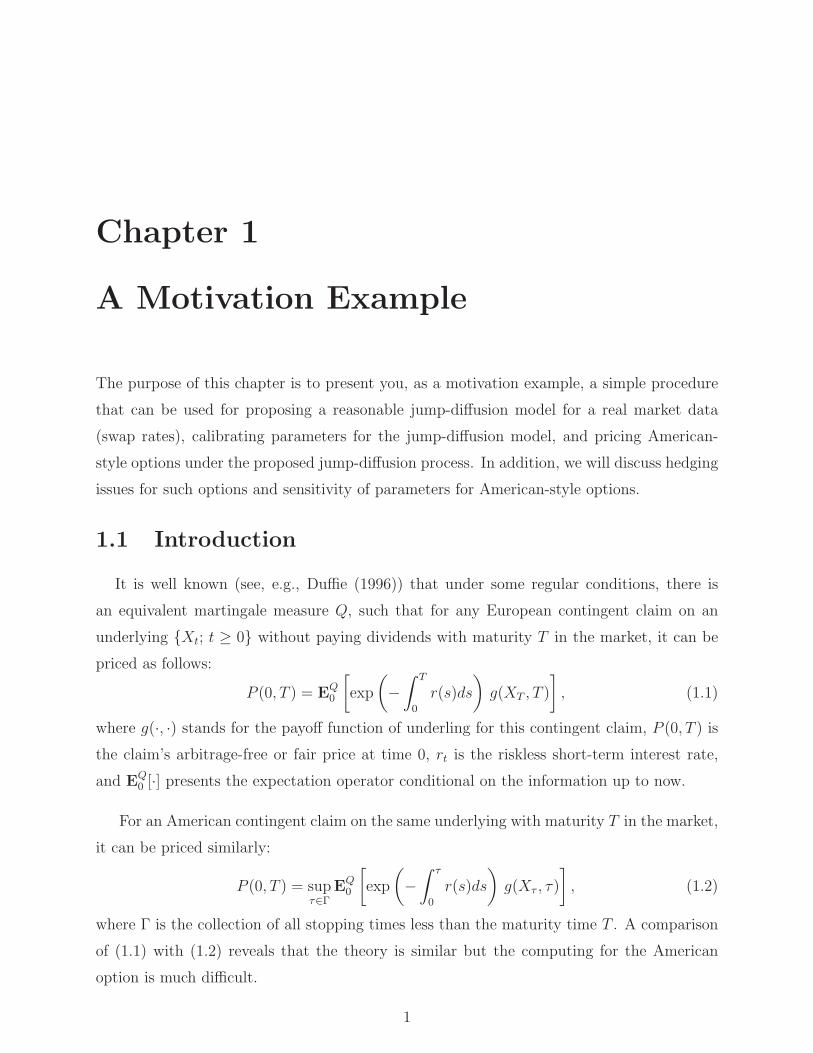
The purpose of this chapter is to present you, as a motivation example, a simple procedure
that can be used for proposing a reasonable jump-diffusion model for a real market data
(swap rates), calibrating parameters for the jump-diffusion model, and pricing American-
style options under the proposed jump-diffusion process. In addition, we will discuss hedging
issues for such options and sensitivity of parameters for American-style options.
1.1 Introduction
It is well known (see, e.g., Duffie (1996)) that under some regular conditions, there is
an equivalent martingale measure Q, such that for any European contingent claim on an
underlying Xt; t ≥ 0 without paying dividends with maturity T in the market, it can be
priced as follows:
P (0, T ) = EQ0
[exp
(−∫ T
0
r(s)ds
)g(XT , T )
], (1.1)
where g(·, ·) stands for the payoff function of underling for this contingent claim, P (0, T ) is
the claim’s arbitrage-free or fair price at time 0, rt is the riskless short-term interest rate,
and EQ0 [·] presents the expectation operator conditional on the information up to now.
For an American contingent claim on the same underlying with maturity T in the market,
it can be priced similarly:
P (0, T ) = supτ∈Γ
EQ0
[exp
(−∫ τ
0
r(s)ds
)g(Xτ , τ)
], (1.2)
where Γ is the collection of all stopping times less than the maturity time T . A comparison
of (1.1) with (1.2) reveals that the theory is similar but the computing for the American
option is much difficult.
1

CHAPTER 1. A MOTIVATION EXAMPLE 2
This theory provides us a “risk neutral” scheme to price any contingent claim. More
precisely, we can pretend to live a risk neutral world to modelling and calibrating parameters
using the data “lived” in the real world, then we do pricing using equation (1.1) or (1.2).
We will use this scheme throughout this paper.
In this chapter, we will present a simple procedure that can be used for proposing a
reasonable jump-diffusion model for a real market data, calibrating parameters for the jump-
diffusion model, and pricing American-style options under the proposed jump-diffusion pro-
cess. In addition, we will discuss hedging issues for such options and sensitivity of parameters
for American-style options. The remainder of the chapter is structured as follows. Section 2
presents some empirical properties of the data by graphing, mining data, and doing some pre-
liminary statistical analysis. Section 3 provides a jump-diffusion model based on the given
properties observed from Section 2, a calibration of parameters under this jump-diffusion
setting by MLE method, and a test for the existence of “jump”. Section 4 proposes a uni-
versal algorithm for American-style options with one-factor underlying model, and uses this
algorithm to price American option for the real data. Section 5 presents hedging issues for
the given American option. Section 6 concludes this chapter and discusses an extension of
our model to a more general tractable jump-diffusion setting called “affine jump-diffusion”
model proposed by Duffie, Pan and Singleton (2000).
1.2 Preliminary Statistical Analysis
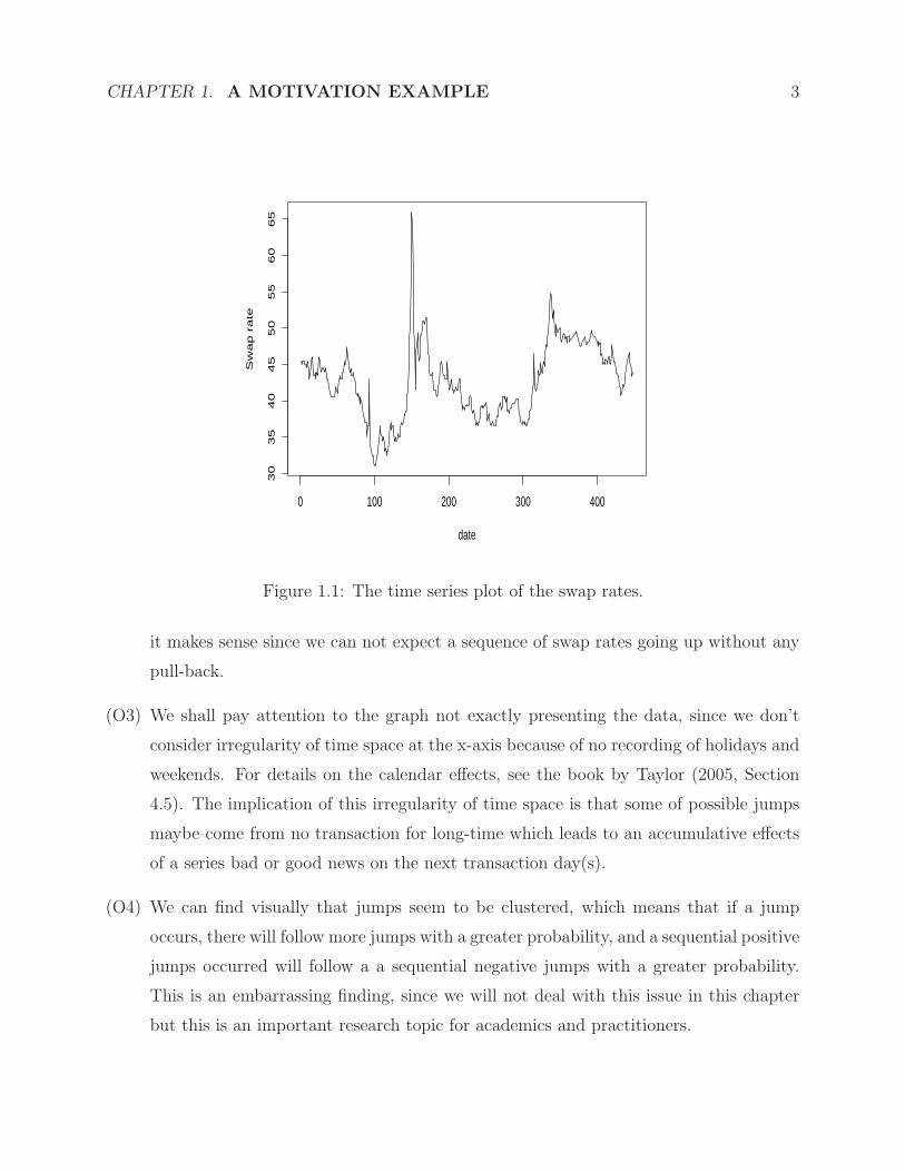
The data we will investigate is a collection of swap rates (the differences between 10 years
LIBOR rates and 10-year treasury bond’s yields) from December 19, 2002 to October 15,
2004. We can present the data graphically in Figure 1.1 by the time series plot. From the
graph, we observe the followings:
(O1) We can visually find there are some possible jumps for swap rates, and jumps seem
to have almost same frequencies for positive and negative jumps. In addition, from
economic standpoint of view, the difference of LIBOR and treasury yield should always
be positive since the former always includes some credit issues.
(O2) We can find “mean reversion” from the graph, which means a very high swap rate tends
to go lower, while a low swap rate tends to bounce back to a higher level. Economically,
CHAPTER 1. A MOTIVATION EXAMPLE 3
0 100 200 300 400
30
35
40
45
50
55
60
65
date
Sw
ap
ra
te
Figure 1.1: The time series plot of the swap rates.
it makes sense since we can not expect a sequence of swap rates going up without any
pull-back.
(O3) We shall pay attention to the graph not exactly presenting the data, since we don’t
consider irregularity of time space at the x-axis because of no recording of holidays and
weekends. For details on the calendar effects, see the book by Taylor (2005, Section
4.5). The implication of this irregularity of time space is that some of possible jumps
maybe come from no transaction for long-time which leads to an accumulative effects
of a series bad or good news on the next transaction day(s).
(O4) We can find visually that jumps seem to be clustered, which means that if a jump
occurs, there will follow more jumps with a greater probability, and a sequential positive
jumps occurred will follow a a sequential negative jumps with a greater probability.
This is an embarrassing finding, since we will not deal with this issue in this chapter
but this is an important research topic for academics and practitioners.

CHAPTER 1. A MOTIVATION EXAMPLE 4
A formal way to modelling a dynamic system for a necessary positive data is to modelling
the logarithm of the original data. The transformed data is graphed in Figure 1.2: Since our
0 100 200 300 400
3.6
3.8
4.0
4.2
date
Log
of S
wap
Rat
e
Figure 1.2: The time series plot of the log of swap rates.
objective is to modelling a dynamic mechanism of the evolution of swap rates, we propose a
general stochastic differential equation to the transformed variable (logarithm of swap rate)
which can usually be called “state” variable. Let St be the swap rate at time t, and denote
Xt as the logarithm of St, namely, Xt = log(St). The general stochastic differential equation
(SDE, or called Black-Scholes model) of Xt is as follows,
dXt = µ(Xt)dt+ σ(Xt)dWt + dJt, X0 = x0, (1.3)
where µ(·) (drift) and σ(·) (diffusion) stand for instantaneous mean function and volatility
function of the process respectively and Wt and Jt are a standard Brownian motion and a
pure jump process respectively.
The objective of modelling, in fact, is to specify the explicit forms of µ(·) and σ(·), andprobability mechanism of pure jump process Jt. In this section, we will have some idea about
the possible shape of σ(·) by a preliminary approximation of the SDE and the transformed
CHAPTER 1. A MOTIVATION EXAMPLE 5
data. First, for a very small time interval δt, the SDE can be approximated by a difference
equation (Euler approximation) as follows,
Xt+δt −Xt ≃ µ(Xt)δt+ σ(Xt)(Wt+δt −Wt) + (Jt+δt − Jt)
≃ σ(Xt)(Wt+δt −Wt) + (Jt+δt − Jt). (1.4)
The reason to omit the term µ(Xt)δt in the above equation is that this term is of the order
of o(1) while other two terms have a lower order. By (1.4), we can have a preliminary
visual sense of the form of σ(·) by looking at the graph of the transformed data with Xt as
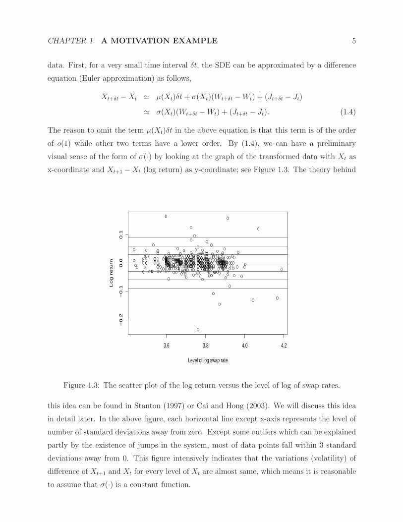
x-coordinate and Xt+1 −Xt (log return) as y-coordinate; see Figure 1.3. The theory behind
3.6 3.8 4.0 4.2
−0
.2−
0.1
0.0
0.1
Level of log swap rate
Lo
g r
etu
rn
Figure 1.3: The scatter plot of the log return versus the level of log of swap rates.
this idea can be found in Stanton (1997) or Cai and Hong (2003). We will discuss this idea
in detail later. In the above figure, each horizontal line except x-axis represents the level of
number of standard deviations away from zero. Except some outliers which can be explained
partly by the existence of jumps in the system, most of data points fall within 3 standard
deviations away from 0. This figure intensively indicates that the variations (volatility) of
difference of Xt+1 and Xt for every level of Xt are almost same, which means it is reasonable
to assume that σ(·) is a constant function.
CHAPTER 1. A MOTIVATION EXAMPLE 6
1.3 Jump-Diffusion Modeling Procedures
By regularities observed in Section 2, we can specify our model under the so-called “equiva-
lent martingale measure” Q (see, e.g., Duffie (1996)) as follows:
(M1). We assume the volatility function σ(·) is a constant function, namely
σ(x) = σ, x ≥ 0 (1.5)
(M2). By (O2) in Section 2, we assume the instantaneous mean function µ(x) is an affine
function,
µ(x) = A(x− x), x ≥ 0, (1.6)
where x stands for long-term mean of the process, and A > 0 is the “speed” of process
back to the long-term mean x. We will explain more about these two parameters.
(M3). We assume the pure jump process Jt is a compound Poisson process independent
of continuous part of Xt and Wt; t ≥ 0 although this assumption might not be
necessary. More formally, we assume that the intensity of the Poisson process is a
constant λ and jump sizes are i.i.d with same distribution η. From (O1) in Section 2,
we can assume that η is a normal distribution, with mean 0, and standard deviation σJ
although the normality assumption on jump sizes might not be appropriate due to its
lack of fat-tail (One can assume that it follows a double exponential as in Kou (2002)
or Tsay (2002, 2005, Section 6.9)).
By assumptions (M1)-(M3) above, we can reformulate (1.3) as follows:
dXt = A(x−Xt)dt+ σdWt + dJt, X0 = x0, (1.7)
where the compensator measure of Jt, ν satisfies:
ν(de, dt) =λ√2πσ2
J
exp
(− e2
2σ2J
)dedt, (1.8)
and
EQ[dWt dJs] = 0, s, t ≥ 0. (1.9)
Using the Ito lemma for semi-martingale, we can solve the equation (1.7) explicitly. That
is, for any given times t and T (we always assume t ≤ T in the following), we have,
XT = Xte−A(T−t) + x
(1− e−A(T−t)
)+ e−A(T−t)
[σ
∫ T
t
eA(s−t)dWs +
∫ T
t
eA(s−t)dJs
].(1.10)

CHAPTER 1. A MOTIVATION EXAMPLE 7
By taking the expectation on both sides of (1.10), we obtain
EQ[XT ] = EQ[Xt]e−A(T−t) + x
(1− e−A(T−t)
). (1.11)
Since A > 0, when T − t → ∞, the first term on the right side of (1.11) will diminish to 0,
while EQ[XT ] → x with exponential rate A. These facts tell us why x is called “long-term
mean” and A is called the “speed” of process back to the long-term mean.
Suppose that the times of observations of the process are equally-spaced, namely, we
assume we observe the process at the regular times to observe data (Xt1 , Xt2 , . . . , XtN+1),
(for notational simplicity, we will denote Xn = Xtn for 1 ≤ n ≤ N + 1 ), where the equal
time interval is defined as ∆ = tn+1 − tn. Then (X1, X2, . . . , XN+1) follows an AR(1) model;
that is,
Xn+1 = a+ bXn + εn+1, 1 ≤ n ≤ N, (1.12)
where
a = x(1− e−A∆), b = e−A∆, (1.13)
and
εn ∼ σe−A∆
∫ ∆
0
eAsdWs + e−A∆
∫ ∆
0
eAsdJs i.i.d. (1.14)
Using (1.12), (1.13) and (1.14), to overcome “curse of dimensionality” for estimating pro-
cedure, we propose the so called “two-stage” estimating technique to obtain preliminary
estimate for parameters. Formally speaking, we first estimate parameters A and x by using
Weighted Least Square method, then use residuals to implement MLE estimating procedure
to estimate λ, σ and σJ . So only thing left we need to do is to find the probability density
function for εn, which is given by the following,
fεn(x) =e−λ∆
√σ2
2A(1− e−2A∆)
φ
x√
σ2
2A(1− e−2A∆)
+∞∑
k=1
e−λ∆λk
k!
∫ ∆
0
. . .
∫ ∆
0
1√σ2
2A(1− e−2A∆) +
∑kl=1 e
−2A(∆−sl)σ2J
×φ
x√
σ2
2A(1− e−2A∆) +
∑kl=1 e
−2A(∆−sl)σ2J
ds1 . . . dsk, (1.15)
where φ(x) = 1√2πe−
x2
2 , namely, the p.d.f of standard normal distribution.
CHAPTER 1. A MOTIVATION EXAMPLE 8
The two-stage estimate for parameters then can be numerically implemented. To estimate
parameters more efficiently, we shall use the whole MLE procedure using Newton-Raphson
algorithm with Two-Stage estimate as initial point of algorithm. Our Two-stage estimates
(based on daily) are as follows:
A = 0.03110101 x = 3.743758 σ = 0.01841 λ = 0.06385 σJ = 0.09299. (1.16)
Our whole MLE estimates (based on daily) are as follows:
A = 0.017124 x = 3.73213 σ = 0.018181 λ = 0.064548 σJ = 0.092432 (1.17)
Now we turn to testing whether the jump diffusion model is adequate. For testing pa-
rameters, we only do test for λ. Equivalently, it tests whether there are jumps for swap rates’
evolution. Remaining parameters’ test can be done similarly. This statistical hypothesis can
be formulated as follows:
H0 : λ = 0 versus H1 : λ > 0. (1.18)
We use the likelihood ratio method to test this hypothesis. It is well known that 2 times
the difference of two maximum log likelihoods converges asymptotically to a χ2-distribution
with degree of freedom equal to difference of dimensions of two parameter spaces. In this
hypothesis, the degree of freedom is 2 since λ = 0 makes σJ irrelevant to the process. We
find that p-value of test statistic is much less than 0.001, which means that H0 is rejected.
So a model for this dataset without jump could be inappropriate.
1.4 Pricing American-style Options Using Stratifica-
tion Simulation Method
To price an American option by using a simulation method (see, e.g., Glasserman, 2004),
it is always approximated by reducing the American option with intrinsic infinite exercise
opportunities into a “Bermudan” option with finite exercise opportunities. Suppose the ap-
proximated “Bermudan” option can be exercised only at a fixed set of exercise opportunities
t1 < t2 < . . . < tm, which are often equally spaced, and underlying process is denoted by
Xt; t ≥ 0. To reduce notation, we write Xti as Xi. Then, if Xt is a Markov process,
Xi; 0 ≤ i ≤ m is a Markov chain, where X0 denotes an initial state of the underlying. Let
hi denote the payoff function for exercise at ti, which is allowed to depend on i. Let Vi(x)
CHAPTER 1. A MOTIVATION EXAMPLE 9
denote the value of the option at ti given Xi = x. By assuming the option has not previ-
ously been exercised, we are ultimately interested in V0(X0). This value can be determined
recursively as follows:
Vm(x) = hm(x) (1.19)
and
Vi−1(x) = maxhi−1(x),E
Q[Di−1,i(Xi)Vi(Xi)|Xi−1 = x], (1.20)
where i = 1, 2, . . . ,m, and Di−1,i(Xi) stands for the discount factor from ti−1 to ti, which
could have the form as
Di−1,i(Xi) = exp
(−∫ ti
ti−1
r(u)du
). (1.21)
So for simulation, the main job will be on implementing (1.20), and main difficulty is also
at here. Actually, if the underlying state is of one dimension, for instance in our setting,
then we can efficiently implement (1.20) by stratification method. That is, we discretize not
only time-dimension but also state space. Formally speaking, for each exercise date ti, let
Ai1, . . . , Aibi be a partition of the state space of Xi into bi subsets. For the initial time 0,
take b0 = 1 and A01 = X0. Define transition probabilities
pij,k = PQ(Xi+1 ∈ Ai+1,k|Xi ∈ Aij) (1.22)
for all j = 1, . . . , bi, k = 1, . . . , bi+1, and i = 0, . . . ,m − 1. (This is taken to be 0 if
PQ(Xi ∈ Aij) = 0.) For each i = 1, . . . ,m and j = 1, . . . , bi, we also define
hi,j = EQ[hi(Xi)|Xi ∈ Aij] (1.23)
takeing this to be 0 if PQ(Xi ∈ Aij) = 0. Now we consider the backward induction
Vij = max
hij,
bi+1∑
k=1
pijkVi+1,k
(1.24)
for all j = 1, . . . , bi, k = 1, . . . , bi+1, and i = 0, . . . ,m − 1, initialized with Vmj = hmj. This
method takes the value V01 calculated through (1.24) as an approximation to V0(X0).
To implement this method, we need to do following steps:
(A1) Simulate a reasonably large number of replications of the Markov chainX0, X1, . . . , Xm.
(A2) Record N ijk, the number of paths that move from Aij to Ai+1,k, for all i = 0, . . . ,m−1,
j = 1, . . . , bi and k = 1, . . . , bi+1.
CHAPTER 1. A MOTIVATION EXAMPLE 10
(A3) Calculate the estimates
pij,k = N ij,k/(N
ij,1 + . . .+N i
j,bi) (1.25)
taking the ratio to be 0 whenever the denominator is 0. And calculate hi,j as the
average value of h(Xi) over those replications in which Xi ∈ Aij, taking it to be 0
whenever there is no path in which Xi ∈ Aij.
(A4) Set Vmj = hmj for all j = 1, . . . , bm, and recursively calculate
Vij = max
hij,
bi+1∑
k=1
pijkVi+1,k
(1.26)
for all j = 1, . . . , bi, and i = 0, . . . ,m− 1. Then V01 just be our estimate of V01.
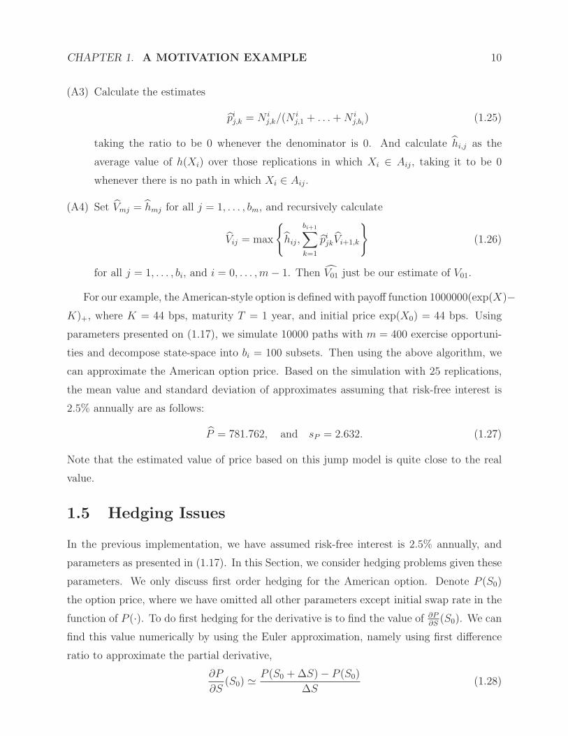
For our example, the American-style option is defined with payoff function 1000000(exp(X)−K)+, where K = 44 bps, maturity T = 1 year, and initial price exp(X0) = 44 bps. Using
parameters presented on (1.17), we simulate 10000 paths with m = 400 exercise opportuni-
ties and decompose state-space into bi = 100 subsets. Then using the above algorithm, we
can approximate the American option price. Based on the simulation with 25 replications,
the mean value and standard deviation of approximates assuming that risk-free interest is
2.5% annually are as follows:
P = 781.762, and sP = 2.632. (1.27)
Note that the estimated value of price based on this jump model is quite close to the real
value.
1.5 Hedging Issues
In the previous implementation, we have assumed risk-free interest is 2.5% annually, and
parameters as presented in (1.17). In this Section, we consider hedging problems given these
parameters. We only discuss first order hedging for the American option. Denote P (S0)
the option price, where we have omitted all other parameters except initial swap rate in the
function of P (·). To do first hedging for the derivative is to find the value of ∂P∂S
(S0). We can
find this value numerically by using the Euler approximation, namely using first difference
ratio to approximate the partial derivative,
∂P
∂S(S0) ≃
P (S0 +∆S)− P (S0)
∆S(1.28)
CHAPTER 1. A MOTIVATION EXAMPLE 11
Then we can use simulation method to find P (S0+∆S) for sufficiently small ∆S so that we
can find an approximate “hedging ratio”. For our example, we let ∆S = ±0.25 bps. The
simulated “hedging ratio” is 0.2515. We can use similar technique to find other “Greek”s.
1.6 Conclusions
We present a whole procedure of modelling, estimating, pricing, and hedging for a real
data under a simple jump-diffusion setting. Some shortcomings are obvious in our setting,
since we don’t consider some issues which maybe important for the price of this option.
For instance, we assume interest rate is deterministic, and intensity λ of “jump event” is
constant. Most critically, we don’t deal with the issue observed on (O4) presented on Section
2. But, sometimes we need to compromise between accuracy and tractability in practice,
since calibrating a jump-diffusion model usually needs a large scale of calculating efforts. A
reasonable extension (still no touch on (O4)) to our model is to take so called “multi-factor”
models, which usually include interest rates, CPI, GDP growth rate, volatility, and other
economic variables as factors. See Duffie, Pan, Singleton (2000) for more details.
1.7 References
Cai, Z. and Y. Hong (2003). Nonparametric methods in continuous-time finance: A selectivereview. In Recent Advances and Trends in Nonparametric Statistics (M.G. Akritas andD.M. Politis, eds.), 283-302.
Duffie, D. (2001). Dynamic Asset Pricing Theory, 3th Edition. Princeton University Press,Princeton, NJ.
Duffie, D., J. Pan and K. Singleton (2000). Transform analysis and asset Pricing for affinejump-diffusion. Econometrica, 68, 1343-1376.
Glasserman, P. (2004). Monte Carlo Methods in Financial Engineering. Springer-Verlag,New York.
Kou, S.G. (2002). A jump diffusion model for option pricing. Management Science, 48,1086-1101.
Merton, R.C. (1976). Option pricing when underlying stock return are discontinuous.Journal of Financial Economics, 3, 125-144.
Stanton, R. (1997). A nonparametric model of term structure dynamics and the marketprice of interest rate risk. Journal of Finance, 52, 1973-2002.

CHAPTER 1. A MOTIVATION EXAMPLE 12
Taylor, S. (2005). Asset Price Dynamics, Volatility, And Prediction. Princeton UniversityPress, Princeton, NJ. (Chapter 4)
Tsay, R.S. (2005). Analysis of Financial Time Series, 2th Edition. John Wiley & Sons,New York.
Chapter 2
Basic Concepts of Prices and Returns
2.1 Introduction
Any empirical analysis of the dynamics of asset prices through time requires price data which
raise some of the questions:
1. The first question is where we can find the data. There are many sources of data includ-
ing web sites, commercial vendors, university research centers, and financial markets.
Here are some of them, listed below:
(a) CRSP: http://www.crsp.com (US stocks)
(b) Commodity Systems Inc: http://www.csidata.com (Futures)
(c) Datastream: http://www.datastream.com/product/has/ (Stocks, bonds, curren-
cies, etc.)
(d) IFM (Institute for Financial Markets): http://www.theifm.org (futures, US stocks)
(e) Olsen & Associates: http://www.olsen.ch (Currencies, etc.)
(f) Trades and Quotes DB: http://www.nyse.com/marketinfo (US stocks)
(g) US Federal Reserve: http://www.federalreserve.gov/releases (Currencies, etc.)
(h) Yahoo! (free): http://biz.yahoo.com/r/ (Stocks, many countries)
(i) For downloading the Chinese financial data, please see the file on my home page
http://www.math.uncc.edu/˜ zcai/finance-data.doc which is downloadable.
Further, the high frequency data (tick by tick data) can be downloaded from the
Bloomberg machine located at Room 33 of Friday Building on our campus but you
13
CHAPTER 2. BASIC CONCEPTS OF PRICES AND RETURNS 14
might ask Department of Finance for a help. Finally, you can download some data
through the web site at Wharton Research Data Services (WRDS)
http://wrds.wharton.upenn.edu/index.shtml, which our UNCC subscribes partially.
To log in WRDS, you need to have an account which can be obtained by contacting
Jon Finn through e-mail [email protected] or phone (704) 687-3156.
2. The second question is what the frequency of data is. It depends on what kind of
data you have and what kind of topics you are doing. For study of microstructure of
financial market, you need to have high frequency data. For most of studies, you might
need daily/weekly/monthly data.
3. The third one is how many periods (say, years) (the length) of data we need for analysis.
Theoretically, the larger sample size would be better but it might have structural
changes for a long sample period. In other words, the dynamics might change over
time.
4. The last one is how many prices for each period we wish to obtain and what kind of
price we need.
Answer: It depends on the purpose of your study.
2.2 Basic Definitions
First, we introduce some basic concepts, which you might be very familiar with.
2.2.1 Time Value of Money
Consider an amount $V invested for n years at a simple interest rate of r per annum (where
r is expressed as a decimal). If compounding takes place only at the end of the year, the
future value after n years is:
FVn = V × (1 + r)n.
If interest is paid m times per year then the future value after n years is:
FV mn = V × (1 +
r
m)m×n.
CHAPTER 2. BASIC CONCEPTS OF PRICES AND RETURNS 15
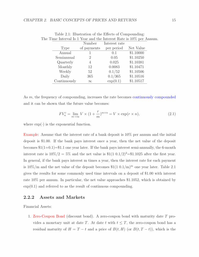
Table 2.1: Illustration of the Effects of Compounding:The Time Interval Is 1 Year and the Interest Rate is 10% per Annum.
Number Interest rateType of payments per period Net ValueAnnual 1 0.1 $1.10000
Semiannual 2 0.05 $1.10250Quarterly 4 0.025 $1.10381Monthly 12 0.0083 $1.10471Weekly 52 0.1/52 $1.10506Daily 365 0.1/365 $1.10516
Continuously ∞ exp(0.1) $1.10517
As m, the frequency of compounding, increases the rate becomes continuously compounded
and it can be shown that the future value becomes:
FV cn = lim
m→∞V × (1 +
r
m)m×n = V × exp(r × n), (2.1)
where exp(·) is the exponential function.
Example: Assume that the interest rate of a bank deposit is 10% per annum and the initial
deposit is $1.00. If the bank pays interest once a year, then the net value of the deposit
becomes $1(1+0.1)=$1.1 one year later. If the bank pays interest semi-annually, the 6-month
interest rate is 10%/2 = 5% and the net value is $1(1 0.1/2)2=$1.1025 after the first year.
In general, if the bank pays interest m times a year, then the interest rate for each payment
is 10%/m and the net value of the deposit becomes $1(1 0.1/m)m one year later. Table 2.1
gives the results for some commonly used time intervals on a deposit of $1.00 with interest
rate 10% per annum. In particular, the net value approaches $1.1052, which is obtained by
exp(0.1) and referred to as the result of continuous compounding.
2.2.2 Assets and Markets
Financial Assets:
1. Zero-Coupon Bond (discount bond). A zero-coupon bond with maturity date T pro-
vides a monetary unit at date T . At date t with t ≤ T , the zero-coupon bond has a
residual maturity of H = T − t and a price of B(t,H) (or B(t, T − t)), which is the
CHAPTER 2. BASIC CONCEPTS OF PRICES AND RETURNS 16
price at time t,
B(t, T ) =
(1 + r)−(T−t) pay at the end of maturity day(1 + r/m)−m(T−t) compounding with frequency mexp(−r(T − t)) continuous compounding
where r is the interest rate. In particular, B(0, T ) is the current, time 0 of the bond,
and B(T, T ) = 1 is equal to the face value, which is a certain amount of money that
the issuing institute (for example, a government, a bank or a company) promises to
exchange the bond for.
2. Coupon Bond. Bonds promising a sequence of payments are called coupon bonds. The
price pt at which the coupon bond is traded at any date t between 0 and the maturity
date T differs from the issuing price p0.
3. Stocks
4. Buying and Selling Foreign Currency
5. Options
6. More · · ·
For more details about bonds, see the book by Capinski and Zastawniak (2003).
2.2.3 Financial Theory
Basic theoretical concepts in financial theory (The best book for this aspect is the book by
Cochrane (2002)):
1. Equilibrium Models. (CAPM, CCAPM, market microstructure theory). Our focus
is only on the CAPM. Please read the paper by Cai and Kuan (2008) and the references
therein on the recent developments in the conditional CAP/APT models. Also, for the
market microstructure theory, please read Chapter 3 of Campbell, Lo and MacKinlay
(1997, CLM hereafter), or Part IV of Taylor (2005), or Chapter 5 of Tsay (2005).
2. Absence of Arbitrage Opportunity. The theory is based on the assumption that it
is impossible to achieve sure, strictly positive, gain with a zero initial endowment. This
assumption suggests imposing deterministic inequality restrictions on asses prices.
CHAPTER 2. BASIC CONCEPTS OF PRICES AND RETURNS 17
3. Actuarial Approach. This approach assumes a deterministic environment and em-
phasizes the concept of a fair price of financial asset.
Example: The price of stock at period 0 that provides future dividends d1, d2, . . . , dt at
predetermined dates 1, 2, . . . , t has to coincide with the discounted sum of future cash flows:
S0 =∞∑
t=1
dtB(0, t),
where B(0, t) is the price of the zero-coupon bond with maturity t (discount factor). The
actuarial approach is not confirmed by empirical research because it does not take into
account uncertainty.
2.3 Statistical Features
2.3.1 Prices
Prices: closing prices in stock market; currency exchange rates; option prices; more, · · ·.
2.3.2 Frequency of Observations
It depends on the data available and the questions that interest a researcher. The price
interval between prices should be sufficient to ensure that trade occurs in most intervals
and it is preferable that the volume of trade is substantial. Daily data are fine for most of
the applications. Also, it is important to distinguish the price data indexed by transaction
counts from the data indexed by time of associated transactions.
2.3.3 Definition of Returns
The statistical inference on asset prices is complicated because asset price might have non-
stationary behavior (upward and downward movements). One can transform asset prices
into returns, which empirically display more stationary behavior. Also, returns are scale-free
and not limited to the positiveness. You may notice the difference in the behavior of price
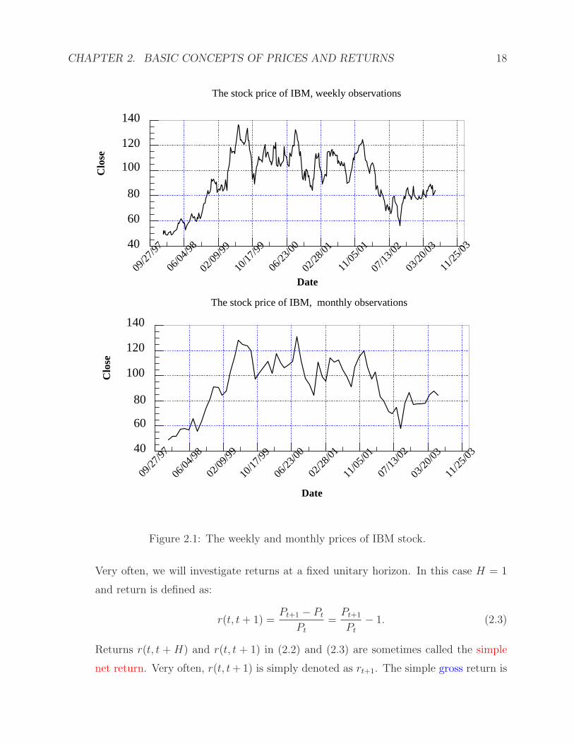
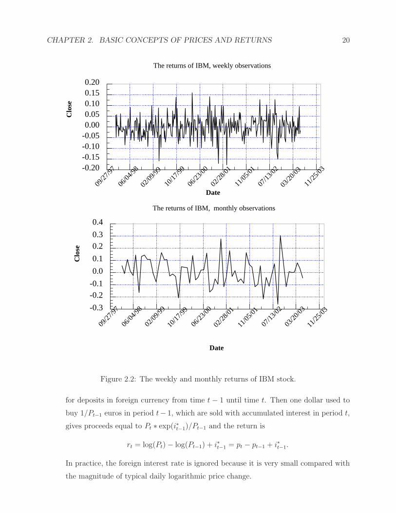
data and returns by looking at IBM prices and IBM returns in Figure 2.1 and Figure 2.2.
1. Return of a financial asset (stock) with price Pt at date t that produces no divi-
dends over the period (t, t+H) is defined as:
r(t, t+H) =Pt+H − Pt
Pt
(2.2)
CHAPTER 2. BASIC CONCEPTS OF PRICES AND RETURNS 18
Date
09/27
/9706
/04/98
02/09
/9910
/17/99
06/23
/0002
/28/01
11/05
/0107
/13/02
03/20
/0311
/25/03
Clo
se
40
60
80
100
120
140
The stock price of IBM, weekly observations
Date
09/27
/9706
/04/98
02/09
/9910
/17/99
06/23
/0002
/28/01
11/05
/0107
/13/02
03/20
/0311
/25/03
Clo
se
40
60
80
100
120
140
The stock price of IBM, monthly observations
Figure 2.1: The weekly and monthly prices of IBM stock.
Very often, we will investigate returns at a fixed unitary horizon. In this case H = 1
and return is defined as:
r(t, t+ 1) =Pt+1 − Pt
Pt
=Pt+1
Pt
− 1. (2.3)
Returns r(t, t + H) and r(t, t + 1) in (2.2) and (2.3) are sometimes called the simple
net return. Very often, r(t, t+1) is simply denoted as rt+1. The simple gross return is
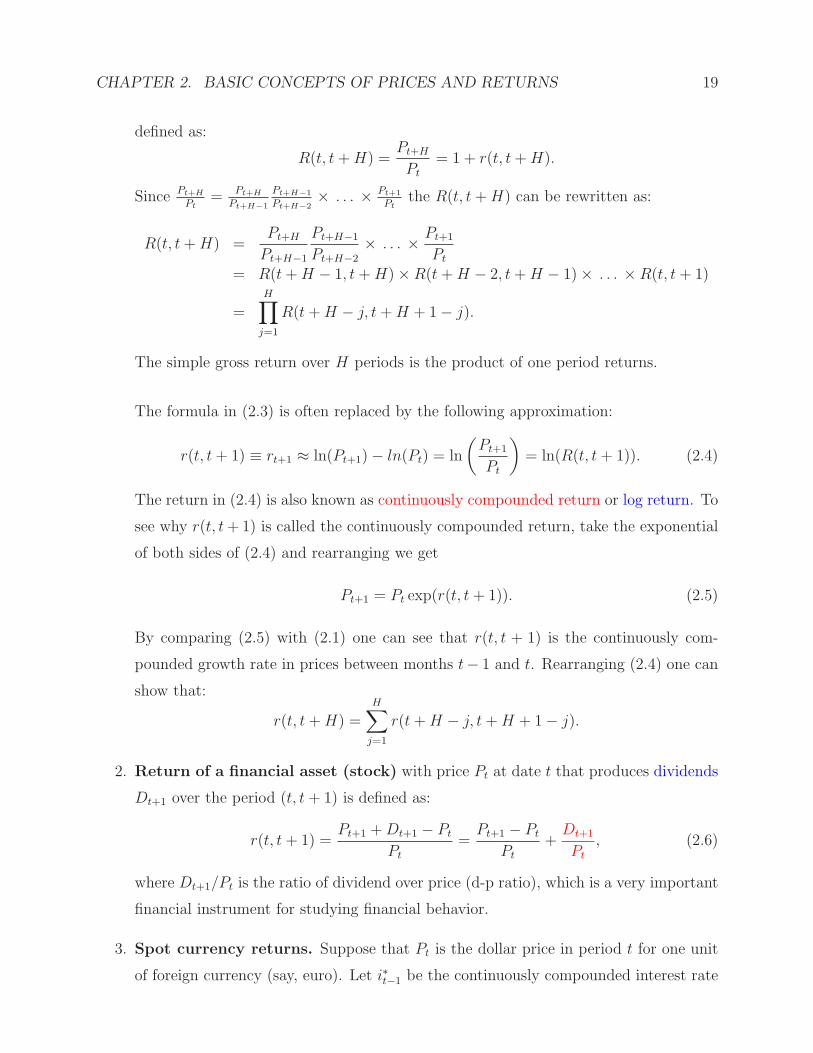
CHAPTER 2. BASIC CONCEPTS OF PRICES AND RETURNS 19
defined as:
R(t, t+H) =Pt+H
Pt
= 1 + r(t, t+H).
Since Pt+H
Pt= Pt+H
Pt+H−1
Pt+H−1
Pt+H−2× . . . × Pt+1
Ptthe R(t, t+H) can be rewritten as:
R(t, t+H) =Pt+H
Pt+H−1
Pt+H−1
Pt+H−2
× . . . × Pt+1
Pt
= R(t+H − 1, t+H)×R(t+H − 2, t+H − 1)× . . . ×R(t, t+ 1)
=H∏
j=1
R(t+H − j, t+H + 1− j).
The simple gross return over H periods is the product of one period returns.
The formula in (2.3) is often replaced by the following approximation:
r(t, t+ 1) ≡ rt+1 ≈ ln(Pt+1)− ln(Pt) = ln
(Pt+1
Pt
)= ln(R(t, t+ 1)). (2.4)
The return in (2.4) is also known as continuously compounded return or log return. To
see why r(t, t+ 1) is called the continuously compounded return, take the exponential
of both sides of (2.4) and rearranging we get
Pt+1 = Pt exp(r(t, t+ 1)). (2.5)
By comparing (2.5) with (2.1) one can see that r(t, t + 1) is the continuously com-
pounded growth rate in prices between months t− 1 and t. Rearranging (2.4) one can
show that:
r(t, t+H) =H∑
j=1
r(t+H − j, t+H + 1− j).
2. Return of a financial asset (stock) with price Pt at date t that produces dividends
Dt+1 over the period (t, t+ 1) is defined as:
r(t, t+ 1) =Pt+1 +Dt+1 − Pt
Pt
=Pt+1 − Pt
Pt
+Dt+1
Pt
, (2.6)
where Dt+1/Pt is the ratio of dividend over price (d-p ratio), which is a very important
financial instrument for studying financial behavior.
3. Spot currency returns. Suppose that Pt is the dollar price in period t for one unit
of foreign currency (say, euro). Let i∗t−1 be the continuously compounded interest rate
CHAPTER 2. BASIC CONCEPTS OF PRICES AND RETURNS 20
Date
09/27
/9706
/04/98
02/09
/9910
/17/99
06/23
/0002
/28/01
11/05
/0107
/13/02
03/20
/0311
/25/03
Clo
se
-0.20-0.15-0.10-0.050.000.050.100.150.20
The returns of IBM, weekly observations
Date
09/27
/9706
/04/98
02/09
/9910
/17/99
06/23
/0002
/28/01
11/05
/0107
/13/02
03/20
/0311
/25/03
Clo
se
-0.3
-0.2-0.1
0.0
0.1
0.20.3
0.4
The returns of IBM, monthly observations
Figure 2.2: The weekly and monthly returns of IBM stock.
for deposits in foreign currency from time t− 1 until time t. Then one dollar used to
buy 1/Pt−1 euros in period t− 1, which are sold with accumulated interest in period t,
gives proceeds equal to Pt ∗ exp(i∗t−1)/Pt−1 and the return is
rt = log(Pt)− log(Pt−1) + i∗t−1 = pt − pt−1 + i∗t−1.
In practice, the foreign interest rate is ignored because it is very small compared with
the magnitude of typical daily logarithmic price change.
CHAPTER 2. BASIC CONCEPTS OF PRICES AND RETURNS 21
4. Futures returns. Suppose Ft,T is the futures price in period t for delivery or cash set-
tlement in some later period T . As there are no dividend payouts on futures contracts,
the futures return is defined as:
rt = log(Ft,T )− log(Ft−1,T ) = ft,T − ft−1,T ,
where ft,T = log(Ft,T ).
5. Excess return is defined as the difference between the asset’s return and the return
on some reference asset. The reference asset is usually assumed to be riskless and in
practice is usually a short-term Treasury bill return. Excess return is defied as:
z(t, t+ 1) = zt+1 = r(t, t+ 1)− r0(t, t+ 1), (2.7)
where r0(t, t+ 1) is the reference return from period t to period t+ 1.
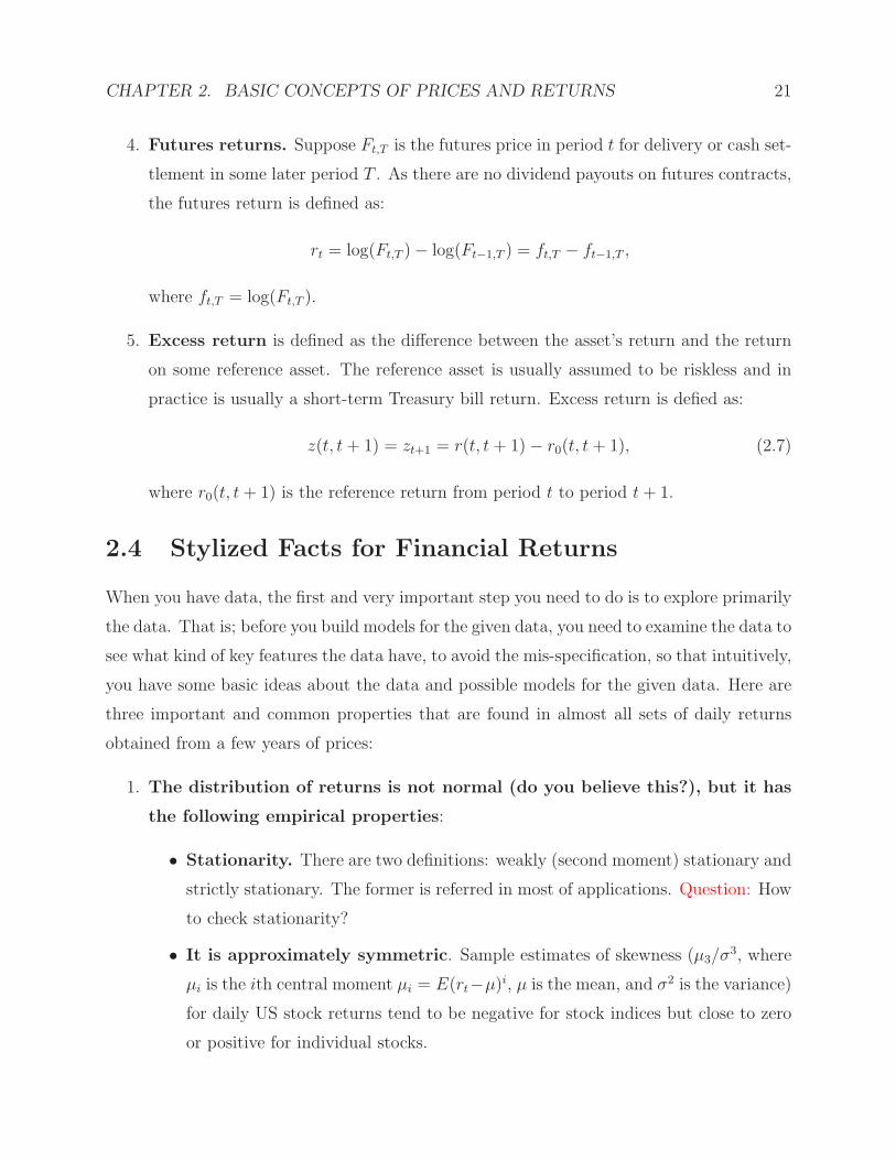
2.4 Stylized Facts for Financial Returns
When you have data, the first and very important step you need to do is to explore primarily
the data. That is; before you build models for the given data, you need to examine the data to
see what kind of key features the data have, to avoid the mis-specification, so that intuitively,
you have some basic ideas about the data and possible models for the given data. Here are
three important and common properties that are found in almost all sets of daily returns
obtained from a few years of prices:
1. The distribution of returns is not normal (do you believe this?), but it has
the following empirical properties:
• Stationarity. There are two definitions: weakly (second moment) stationary and
strictly stationary. The former is referred in most of applications. Question: How
to check stationarity?
• It is approximately symmetric. Sample estimates of skewness (µ3/σ3, where
µi is the ith central moment µi = E(rt−µ)i, µ is the mean, and σ2 is the variance)
for daily US stock returns tend to be negative for stock indices but close to zero
or positive for individual stocks.

CHAPTER 2. BASIC CONCEPTS OF PRICES AND RETURNS 22
• It has fat tails. Kurtosis (the ratio of the forth central moment over square of
the second central moment minus 3; that is, γ = µ4/µ22 − 3) for daily US stock
returns are large and positive for both indices and individual stocks which means
that returns have more probability mass in the tail areas than would be predicted
by a normal distribution (leptokurtic or γ > 0).
• It has a high peak. See Figure 2.3 for IMB daily returns by a comparison with
the standard norm.
Figures 2.3-2.4 compare empirical estimates of the probability distribution function
−6 −4 −2 0 2 4 60
20
40
60
80Standardized IBM returns
−6 −4 −2 0 2 4 60
0.1
0.2
0.3
0.4
0.5Analytical pdfEmpirical pdf
Figure 2.3: The empirical distribution of standardized IBM daily returns and the pdf of stan-dard normal. Notice fat tails of empirical distribution compared with the tails of standardnormal.
(pdf) of standardized IBM and Microsoft (MSFT) returns, zt = (rt − r)/σ, with the
probability density distribution of normal distribution. This empirical density estimate
CHAPTER 2. BASIC CONCEPTS OF PRICES AND RETURNS 23
−6 −4 −2 0 2 4 60
20
40
60
80
100Standardized MSFT returns
−6 −4 −2 0 2 4 60
0.1
0.2
0.3
0.4
0.5Analytical pdfEmpirical pdf
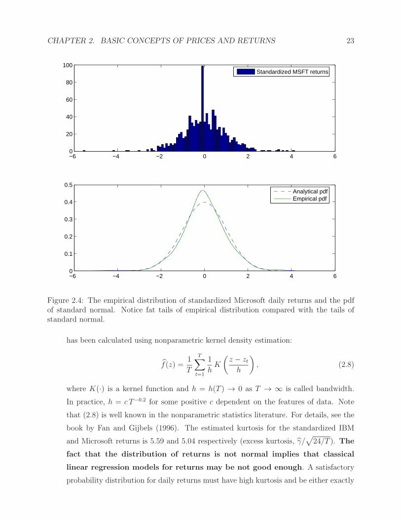
Figure 2.4: The empirical distribution of standardized Microsoft daily returns and the pdfof standard normal. Notice fat tails of empirical distribution compared with the tails ofstandard normal.
has been calculated using nonparametric kernel density estimation:
f(z) =1
T
T∑
t=1
1
hK
(z − zth
), (2.8)
where K(·) is a kernel function and h = h(T ) → 0 as T → ∞ is called bandwidth.
In practice, h = c T−0.2 for some positive c dependent on the features of data. Note
that (2.8) is well known in the nonparametric statistics literature. For details, see the
book by Fan and Gijbels (1996). The estimated kurtosis for the standardized IBM
and Microsoft returns is 5.59 and 5.04 respectively (excess kurtosis, γ/√
24/T ). The
fact that the distribution of returns is not normal implies that classical
linear regression models for returns may be not good enough. A satisfactory
probability distribution for daily returns must have high kurtosis and be either exactly

CHAPTER 2. BASIC CONCEPTS OF PRICES AND RETURNS 24
or approximately symmetric. Figure 2.5 displays the quantile-quantile (Q-Q) plots
for the standardized IBM returns (top panel) and the standardized Microsoft returns
(bottom panel). It is evident that the IBM and MSFT returns are not exactly normally
distributed. For more examples, see Table 1.2 (p. 11) and Figure 1.4 (p.19) in Tsay
(2005) or Table 4.6 and Figures 4.1 and 4.2 (pp 70-72) in Taylor (2005).
−4 −3 −2 −1 0 1 2 3 4−6
−4
−2
0
2
4
6
Standard Normal Quantiles
Qua
ntile
s of
Inpu
t Sam
ple
QQplot for standardized IBM returns
−4 −3 −2 −1 0 1 2 3 4−6
−4
−2
0
2
4
6
Standard Normal Quantiles
Qua
ntile
s of
Inpu
t Sam
ple
QQplot for standardized MSFT returns
Figure 2.5: Q-Q plots for the standardized IBM returns (top panel) and the standardizedMicrosoft returns (bottom panel).
Question 1: How to model the distribution of a return or returns? (A) Parametric
models; (B) Mixture models (see Section 4.8 in Taylor (2005) and Maheu and McCurdy
(2009)); (C) Nonparametric models.
Question 2: How do you know the distribution of a return belong to a particular family?
(A) Informative way to do a model checking using graphical methods, such as Q-Q plot;

CHAPTER 2. BASIC CONCEPTS OF PRICES AND RETURNS 25
(B) Official way is to do hypothesis testing; say Jarque-Bera test and Kolmogorov-
Smirnov tests or other advanced tests, say nonparametric versus parametric tests.
2. There is almost no correlation between returns for different days. Recall that
the correlation between returns τ periods apart is estimated from T observations by
the sample autocorrelation at lag τ :
ρτ =
∑T−τt=1 (rt − r)(rt+τ − r)∑T
t=1(rt − r)2
where r is the sample mean of all T observations. The command acf() in R is the plot
of ρτ versus τ , which is called the ACF plot.
To test H0 : ρ1 = 0, one can use the Durbin-Watson test statistic which is
DW =T∑
t=2
(rt − rt−1)2/
T∑
t=1
r2t .
Straightforward calculation shows that DW ≈ 2(1− ρ1), where ρ1 is the lag-1 ACF of
rt.
Consider testing that several autocorrelation coefficients are simultaneously zero, i.e.
H0 : ρ1 = ρ2 = . . . = ρm = 0. Under the null hypothesis, it is easy to show (see, Box
and Pierce (1970)) that
Q = T
m∑
k=1
ρ2k −→ χ2m. (2.9)
Ljung and Box (1978) provided the following finite sample correction which yields a
better fit to the χ2m for small sample sizes:
Q∗ = T (T + 2)m∑
k=1
ρ2kT − k
−→ χ2m. (2.10)
Both are called Q-test and well known in the statistics literature. Of course, they are
very useful in applications.
The function in R for the Ljung-Box test is
Box.test(x, lag = 1, type = c("Box-Pierce", "Ljung-Box"))

CHAPTER 2. BASIC CONCEPTS OF PRICES AND RETURNS 26
and the Durbin-Watson test for autocorrelation of disturbances is
dwtest(formula, order.by = NULL, alternative = c("greater","two.sided",
"less"),iterations = 15, exact = NULL, tol = 1e-10, data = list())
which is in the package lmtest.
3. The correlation between magnitudes of returns on nearby days are positive
and statistically significant. Functions of returns can have substantial autocorrela-
tions even though returns have very small autocorrelations. Usually, autocorrelations
are discussed for |rt|λ, λ = 1, 2. It is a stylized fact that there is positive dependence
between absolute returns on nearby days, and likewise for squared returns. See Section
4.10 in Taylor (2005) and Section 3.5.8.
The autocorrelations of absolute returns are always positive at a lag one day and
positive dependence continues to be found for several further lags. Squared returns
also exhibit positive positive dependence but to a lesser degree. The dependence
in absolute returns may be explained by volatility clustering or regime
switching or nonlinearity. See Section 4.9 in Taylor (2005).
4. Nonlinearity of the Returns Process. For example, Hong and Lee (2003) con-
ducted studies on exchange rates and they found that some of them are predictable
based on nonlinear time series models. There are many ongoing research activities in
this direction. See Chapter 4 in Tsay (2005) and Cai and Kuan (2008). If we have
time, we will spend some time in exploring further on this topic.
2.5 Problems
1. Download weekly (daily) price data for any two stocks, for example, IBM stock (P1t)
for 01/02/62 - 01/15/08 and for Microsoft stock (P2t) for 03/13/86 - 01/15/2008.
(a) Create a time series of continuously compounded weekly returns for IBM (r1t)
and for Microsoft (r2t).
(b) Use the constructed weekly returns to construct a series of monthly returns. You
may assume for simplicity that one month consists of four weeks.

CHAPTER 2. BASIC CONCEPTS OF PRICES AND RETURNS 27
(c) Construct a graph of stock price series (P1t, P2t) and returns series (r1t, r2t).
(d) Compute and graph the rolling estimates of the sample mean and variance for
stock prices and returns. In computation of rolling estimates, you may use the
last quarter of data (13 weeks).
NOTE: You either write code by yourself or use the build-in function in R. To use
the build-in function for the rolling analysis in R, you need to do the followings:
The first thing you need to do is to load fTrading, which is a package for RMetrics.
When you open R window, go to packages −→ local packages, and go down
to fTrading, and finally, double click it. After you load the package fTrading, the
command for the rolling analysis is
roll=rollFun(x,n,FUN=mean) # x is the series for the rolling
Or, you can use rapply or rollmean in the package zoo. To use the package zoo,
you need to load it first.
x1=zoo(x)
x2=rapply(x1,n,FUN=mean) # x is the series for the rolling
(e) What is the definition of a stationary stochastic process? Do prices look like a
stationary process? Why? Do returns look like a stationary process? Why?
(f) Compute autocorrelation coefficients ρk for 1 ≤ k ≤ 5 for prices and returns series.
To compute autocorrelation coefficients, you may use the program acf function in
R. This program is called as follows:
rho=acf(x,k, plot=F)
win.graph()
# open a graph window
plot(rho)
# make a plot
rho_value=rho$acf
# get the estimated $\rho$-values
print(rho_value)
# print the estmated $\rho$-values on screen
CHAPTER 2. BASIC CONCEPTS OF PRICES AND RETURNS 28
# where $x$ is a time-series vector (stock prices, stock returns,
# etc.), $k$ is the maximum lag considered ($5$ in this example).
(g) Based on the computed autocorrelations for IBM and MSFT stock prices and
returns, what can you say about correlation between stock prices for different
days? What can you say about correlation between stock returns for different
days?
(h) Using your stock returns for IBM and MSFT, rit, i = 1, 2, construct four more
series yit = |rit|λ, i = 1, 2 and λ = 1, 2. Compute autocorrelation coefficients
ρk for 1 ≤ k ≤ 5 for the newly constructed series. Compare the computed
correlations for |rit|λ, λ = 1, 2, and |rit|. Are results as you expected?
(i) Use the Jarque-Bera test (see Jarque and Bera (1980, 1987)) to test the assump-
tion of return normality for IBM and Microsoft stock returns.
NOTE: The Jarque-Bera test evaluates the hypothesis that X has a normal dis-
tribution with unspecified mean and variance, against the alternative that X does
not have a normal distribution. The test is based on the sample skewness and
kurtosis of X. For a true normal distribution, the sample skewness should be
near 0 and the sample kurtosis should be near 3. A test has the following general
form:
JB =T
6
(Sk +
(K − 3)2
4
)→ χ2
2,
where Sk and K are the measures of skewness and kurtosis respectively. To use
the build-in function for the Jarque-Bera test in R, you need to do the followings:
The first thing you need to do is to load tseries, which is a package for Time
Series and Computational Finance. When you open R window, go to packages
−→ local packages, and go down to tseries, and finally, double click it. After
you load the package tseries, the command for the Jarque-Bera test is
jb=jarque.bera.test(x) # x is the series for the test
print(jb)
Alternatively, you can also use the Kolmogorov-Smirnov tests as
CHAPTER 2. BASIC CONCEPTS OF PRICES AND RETURNS 29
ks.test(x, y, ..., alternative = c("two.sided", "less", "greater"),
exact = NULL)
To use Kolmogorov-Smirnov tests, you need to standardize the data first.
2. Use R program to estimate the probability density function (see (2.8)) of standardized
IBM and MSFT stock returns zit, zit = (rit − ri)/σi, where ri and σi are the sample
mean and standard deviation of ri, i = 1, 2. The program R is called as follows:
Suppose that Z is a vector of standardized stock returns,
y0=density(Z, m=100, from=-3, to=3)
# m is the number of grid points from interval (from, to)
y1=y0$y
# get estimated density vaules at m grid points
x0=seq(-3,3,length=100)
# set the vaules for m grid points
win.graph()
matplot(x0,cbind(y1,dnorm(x0)),type="l", lty=c(1,2),xlab="",ylab="")
# make a plot with two graphs
win.graph()
qqnorm(Z)
qqline(Z,col=2)
# make a Q-Q plot of Z
# where $y1$ is a vector of estimated probabilities at $m=100$
# grid points from $-3$ to $3$. Compare the empirical distribution
# with a graph of standard normal distribution.
(a) Estimate and construct a graph of the estimated probability density function for
IBM and Microsoft stock returns:
(b) On the same graph with the empirical density, construct a graph of the standard
normal density function. Comment your results.
(c) Construct QQ-plot for standardized IBM and MSFT returns. You may use the
R command for this. Comment your results.
CHAPTER 2. BASIC CONCEPTS OF PRICES AND RETURNS 30
2.6 References
Box, G. and D. Pierce (1970). Distribution of residual autocorrelations in autoregressiveintegrated moving average time series models. Journal of the American StatisticalAssociation, 65, 1509-1526.
Cai, Z. and C.-M. Kuan (2008). Time-varying betas models: A nonparametric analysis.Working paper, Department of Mathematics and Statistics, University of North Car-olina at Charlotte.
Campbell, J. Y., A.W. Lo and A.C. MacKinlay (1997). The Econometrics of FinancialMarkets. Princeton University Press, Princeton, NJ. (Chapter 1).
Capinski, M. and T. Zastawniak (2003). Mathematics for Finance. Springer-Verlag, Lon-don.
Cochrane, J.H. (2002). The Asset Pricing Theory. Princeton University Press, Princeton,NJ. (financial theory)
Hong, Y. and T.-H. Lee (2003). Inference on via generalized spectrum and nonlinear timeseries models. The Review of Economics and Statistics, 85, 1048-1062.
Gourieroux, C. and J. Jasiak (2001). Financial Econometrics: Problems, Models, andMethods. Princeton University Press, Princeton, NJ. (Chapter 1)
Fan, J. and I. Gijbels (1996). Local Polynomial Modeling and Its Applications. London:Chapman and Hall.
Jarque, C.M. and A.K. Bera (1980). Efficient tests for normality, homoscedasticity andserial independence of regression residuals. Economics Letters, 6, 255-259.
Jarque, C.M. and A.K. Bera (1987). A test for normality of observations and regressionresiduals. International Statistical Review, 55, 163-172.
Ljung, G. and G. Box (1978). On a measure of lack of fit in time series models. Biometrika,66, 67-72.
Maheu, J.M. and T.H. McCurdy (2009). How Useful are Historical Data for Forecastingthe Long-Run Equity Return Distribution? Journal of Business & Economic Statistics,27, 95-112.
Taylor, S. (2005). Asset Price Dynamics, Volatility, And Prediction. Princeton UniversityPress, Princeton, NJ. (Chapters 1-4)
Tsay, R.S. (2005). Analysis of Financial Time Series, 2th Edition. John Wiley & Sons,New York. (Chapter 1)
Zivot, E. (2002). Lecture Notes on Applied Econometric Modeling in Finance. The weblink is: http://faculty.washington.edu/ezivot/econ483/483notes.htm
Chapter 3
Linear Time Series Models and TheirApplications
In this chapter, we discuss basic theories of linear time series analysis, introduce some simple
econometric models useful for analyzing financial time series, and apply the models to asset
returns. Discussions of the concepts are brief with emphasis on those relevant to financial
applications. Understanding the simple time series models introduced here will go a long
way to better appreciate the more sophisticated financial econometric models of the later
chapters. There are many time series textbooks available. For basic concepts of linear time
series analysis, see Box, Jenkins, and Reinsel (1994, Chapters 2 and 3) and Brockwell and
Davis (1996, Chapters 1).
Treating an asset return (e.g., log return rt of a stock) as a collection of random vari-
ables over time, we have a time series rt. Linear time series analysis provides a natural
framework to study the dynamic structure of such a series. The theories of linear time series
discussed include stationarity, dynamic dependence, autocorrelation function, modeling, and
forecasting. The econometric models introduced include
(a) simple autoregressive (AR) models,
(b) simple moving-average (MA) models,
(c) mixed autoregressive moving-average (ARMA) models,
(d) a simple regression model (constant expected return model) with time series errors,
and
(f) differenced models (ARIMA).
For an asset return rt , simple models attempt to capture the linear relationship between rt
and information available prior to time t. The information may contain the historical values
31
CHAPTER 3. LINEAR TIME SERIES MODELS AND THEIR APPLICATIONS 32
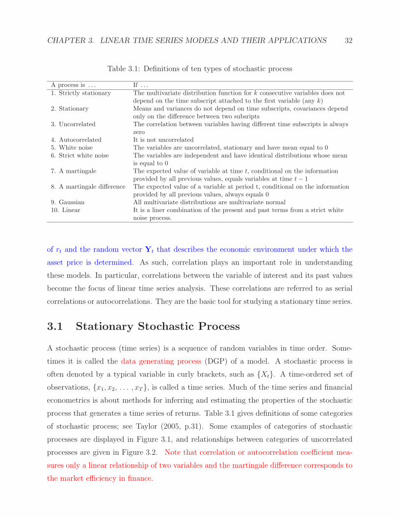
Table 3.1: Definitions of ten types of stochastic process
A process is . . . If . . .1. Strictly stationary The multivariate distribution function for k consecutive variables does not
depend on the time subscript attached to the first variable (any k)2. Stationary Means and variances do not depend on time subscripts, covariances depend
only on the difference between two subsripts3. Uncorrelated The correlation between variables having different time subscripts is always
zero4. Autocorrelated It is not uncorrelated5. White noise The variables are uncorrelated, stationary and have mean equal to 06. Strict white noise The variables are independent and have identical distributions whose mean
is equal to 07. A martingale The expected value of variable at time t, conditional on the information
provided by all previous values, equals variables at time t− 18. A martingale difference The expected value of a variable at period t, conditional on the information
provided by all previous values, always equals 09. Gaussian All multivariate distributions are multivariate normal10. Linear It is a liner combination of the present and past terms from a strict white
noise process.
of rt and the random vector Yt that describes the economic environment under which the
asset price is determined. As such, correlation plays an important role in understanding
these models. In particular, correlations between the variable of interest and its past values
become the focus of linear time series analysis. These correlations are referred to as serial
correlations or autocorrelations. They are the basic tool for studying a stationary time series.
3.1 Stationary Stochastic Process
A stochastic process (time series) is a sequence of random variables in time order. Some-
times it is called the data generating process (DGP) of a model. A stochastic process is
often denoted by a typical variable in curly brackets, such as Xt. A time-ordered set of
observations, x1, x2, . . . , xT, is called a time series. Much of the time series and financial
econometrics is about methods for inferring and estimating the properties of the stochastic
process that generates a time series of returns. Table 3.1 gives definitions of some categories
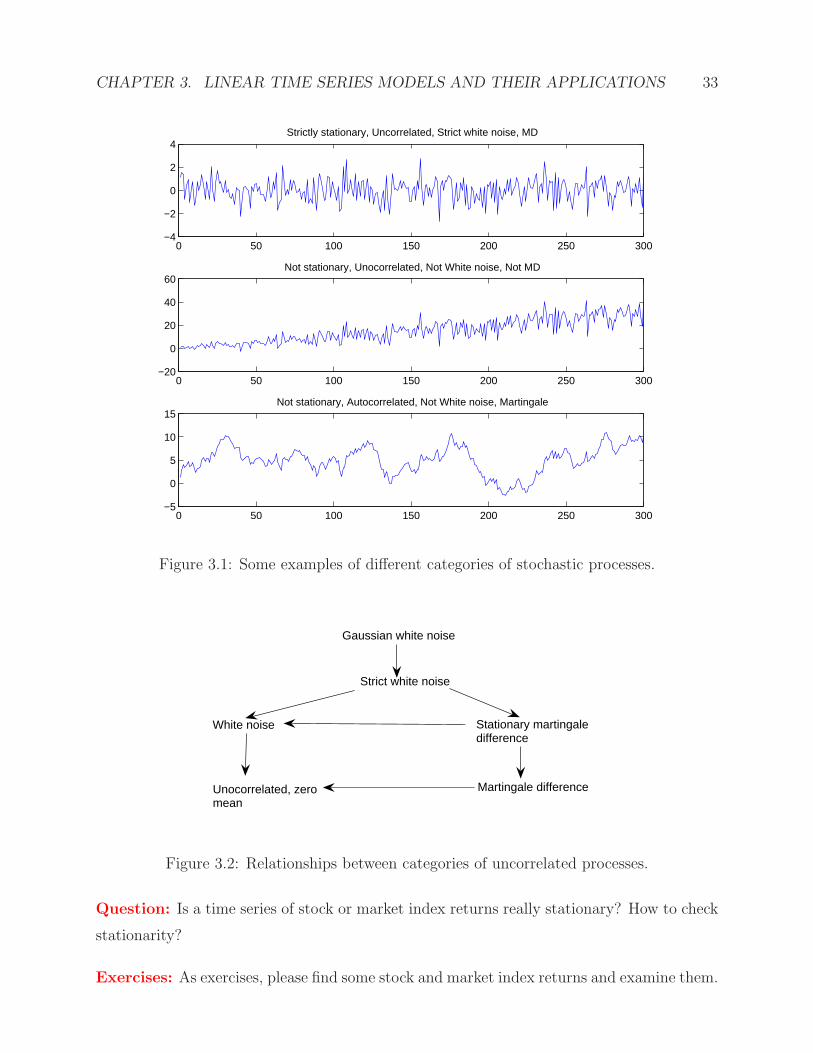
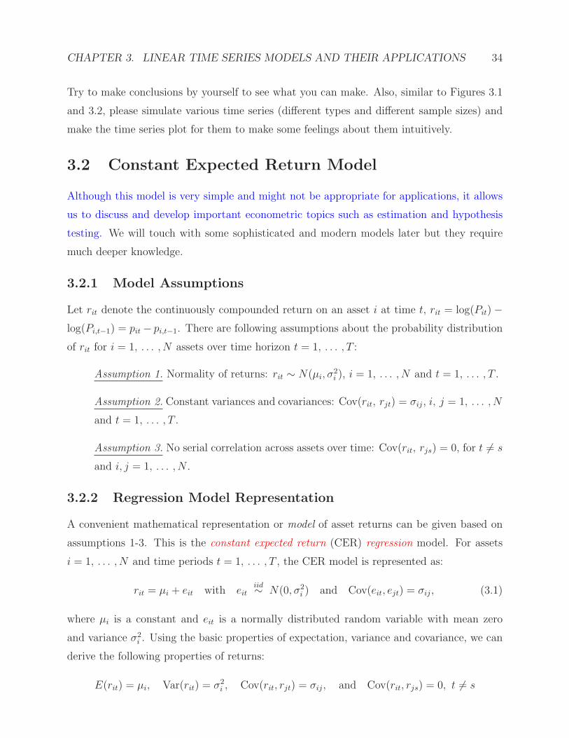
of stochastic process; see Taylor (2005, p.31). Some examples of categories of stochastic
processes are displayed in Figure 3.1, and relationships between categories of uncorrelated
processes are given in Figure 3.2. Note that correlation or autocorrelation coefficient mea-
sures only a linear relationship of two variables and the martingale difference corresponds to
the market efficiency in finance.
CHAPTER 3. LINEAR TIME SERIES MODELS AND THEIR APPLICATIONS 33
0 50 100 150 200 250 300−4
−2
0
2
4Strictly stationary, Uncorrelated, Strict white noise, MD
0 50 100 150 200 250 300−20
0
20
40
60Not stationary, Unocorrelated, Not White noise, Not MD
0 50 100 150 200 250 300−5
0
5
10
15Not stationary, Autocorrelated, Not White noise, Martingale
Figure 3.1: Some examples of different categories of stochastic processes.
Gaussian white noise
Strict white noise
Stationary martingaledifference
White noise
Unocorrelated, zeromean
Martingale difference
Figure 3.2: Relationships between categories of uncorrelated processes.
Question: Is a time series of stock or market index returns really stationary? How to check
stationarity?
Exercises: As exercises, please find some stock and market index returns and examine them.
CHAPTER 3. LINEAR TIME SERIES MODELS AND THEIR APPLICATIONS 34
Try to make conclusions by yourself to see what you can make. Also, similar to Figures 3.1
and 3.2, please simulate various time series (different types and different sample sizes) and
make the time series plot for them to make some feelings about them intuitively.
3.2 Constant Expected Return Model
Although this model is very simple and might not be appropriate for applications, it allows
us to discuss and develop important econometric topics such as estimation and hypothesis
testing. We will touch with some sophisticated and modern models later but they require
much deeper knowledge.
3.2.1 Model Assumptions
Let rit denote the continuously compounded return on an asset i at time t, rit = log(Pit)−log(Pi,t−1) = pit − pi,t−1. There are following assumptions about the probability distribution
of rit for i = 1, . . . , N assets over time horizon t = 1, . . . , T :
Assumption 1. Normality of returns: rit ∼ N(µi, σ2i ), i = 1, . . . , N and t = 1, . . . , T .
Assumption 2. Constant variances and covariances: Cov(rit, rjt) = σij, i, j = 1, . . . , N
and t = 1, . . . , T .
Assumption 3. No serial correlation across assets over time: Cov(rit, rjs) = 0, for t 6= s
and i, j = 1, . . . , N .
3.2.2 Regression Model Representation
A convenient mathematical representation or model of asset returns can be given based on
assumptions 1-3. This is the constant expected return (CER) regression model. For assets
i = 1, . . . , N and time periods t = 1, . . . , T , the CER model is represented as:
rit = µi + eit with eitiid∼ N(0, σ2
i ) and Cov(eit, ejt) = σij , (3.1)
where µi is a constant and eit is a normally distributed random variable with mean zero
and variance σ2i . Using the basic properties of expectation, variance and covariance, we can
derive the following properties of returns:
E(rit) = µi, Var(rit) = σ2i , Cov(rit, rjt) = σij , and Cov(rit, rjs) = 0, t 6= s
CHAPTER 3. LINEAR TIME SERIES MODELS AND THEIR APPLICATIONS 35
so that
Corr(rit, rjt) =σijσiσj
= ρij and Corr(rit, rjs) =0
σiσj= 0, i 6= j, t 6= s.
Since the random variable eit is independent and identically distributed normal the asset
returns rit will also be i.i.d normal:
ritiid∼ N(µi, σ
2i )
Therefore, the CER (3.1) is equivalent to the model implied by assumptions 1-3. The random
variable eit can be interpreted as representing the unexpected news concerning the value of
asset that arrives between times t− 1 and time t:
eit = rit − µi = rit − E(rit).
The assumption that E(eit) = 0 means that news, on average, is neutral. The assumption
that Var(eit) = σ2i can be interpreted as saying that volatility of news arrival is constant
over time.
Question: Do you think that the CER model is a good model for applications? Please
answer this question from the empirical stand point of view.
3.2.3 CER Model of Asset Returns and Random Walk Model ofAsset Prices
The CER model of asset returns (3.1) gives a rise to the random walk (RW) model of the
logarithm of asset prices. Recall that continuously compounded return, rit, is defined as:
ln(Pit)− ln(Pi,t−1) = rit
Letting pit = ln(Pit) and using the representation of rit in the CER model (3.1), we may
rewrite the above as the random walk model (RW)
pit − pi,t−1 = µi + eit (3.2)
In the RW model, µi represents the expected change in the log of asset prices between periods
t − 1 and t and eit represents the unexpected change in prices. The RW model gives the
following interpretation for the evolution of asset prices:
pit = µi + pit−1 + eit, piT = Tµi + pi0 +T∑
t=1
eit.
At time t = 0 the expected price at time t = T is E(piT ) = pi0 + Tµi.

CHAPTER 3. LINEAR TIME SERIES MODELS AND THEIR APPLICATIONS 36
3.2.4 Monte Carlo Simulation Method
A good way to understand the probabilistic behavior of a model is to use simulation methods
to create pseudo data from the model. The process of creating such pseudo data is called
Monte Carlo simulation. The steps to create a Monte Carlo simulation from the CER model
are:
• Fix values for the CER model parameters µ and σ (or σ2).
• Determine the number of simulated values, T , to create.
• Use a computer random number generator to simulate T iid values et from N(0, σ2)
distribution. Denote these simulated values as e∗1, . . . , e∗T .
• Create simulated return data r∗t = µ+ e∗t for t = 1, . . . , T .
The Monte Carlo simulation of returns and prices using the CER model is presented in
Figure 3.3.
Exercises: Please follow the above steps to do some Monte Carlo simulations and make
your conclusions and interpret them.
3.2.5 Estimation
The CER model states that ritiid∼ N(µi, σ
2i ). Our best guess for the return at the end of
the month is E(rit) = µi, our measure of uncertainty about our best guess is captured by
σi =√Var(rit), and our measure of the direction of linear association between rit and rjt
is σij = Cov(rit, rjt). A key task in financial econometrics is estimating the values of µi, σ2i
and σij from the observed historical data. The ordinary least squares (OLS) estimates are:
µi =1
Tι′r =
1
T
T∑
t=1
rit = ri,
σ2i =
1
T − 1(ri − ri)
′(ri − ri) =1
T − 1
T∑
t=1
(rit − ri)2, σi =
√σ2i ,
σij =1
T − 1(ri − ri)
′(rj − rj) =1
T − 1
T∑
t=1
(rit − ri)(rjt − rj), and ρij =σijσiσj
,
where ι is an T × 1 vector of ones, ri = (ri1, ri2, . . . , riT )′ is a T × 1 vector of returns.
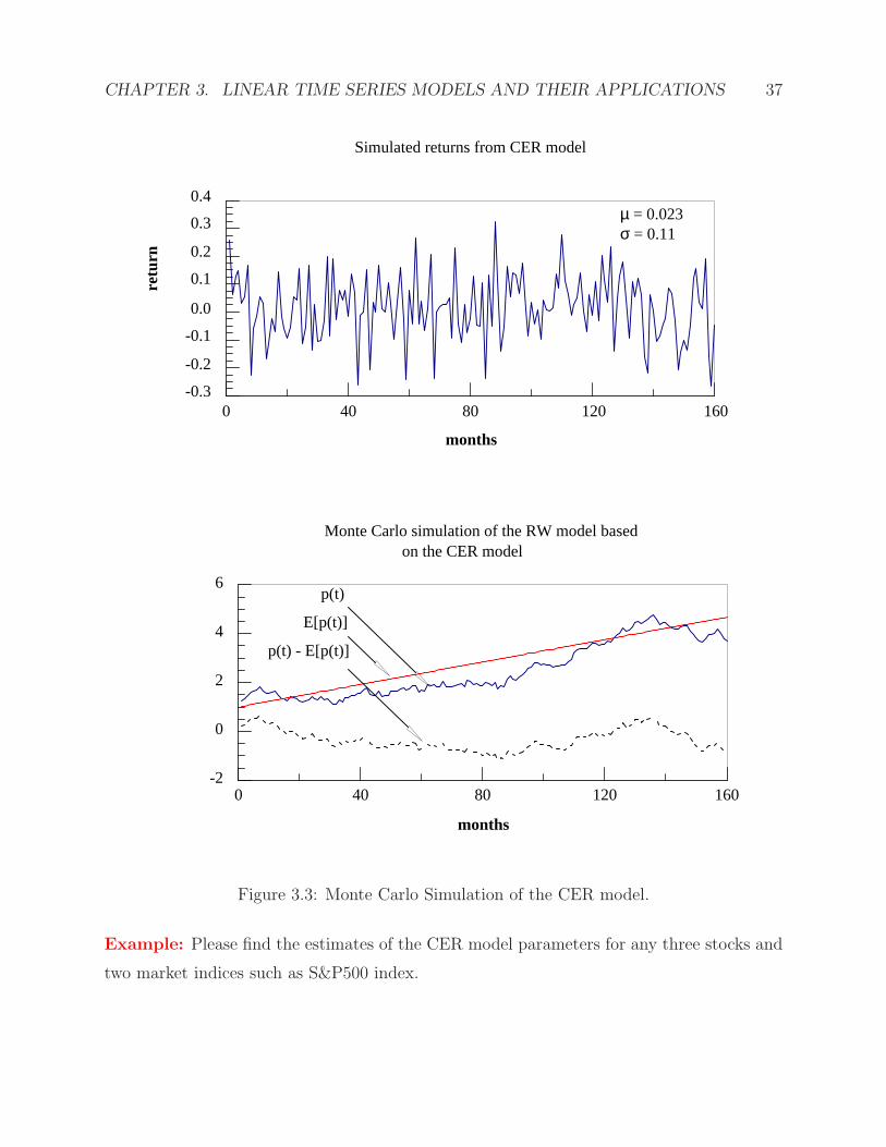
CHAPTER 3. LINEAR TIME SERIES MODELS AND THEIR APPLICATIONS 37
months
0 40 80 120 160
retu
rn
-0.3
-0.2
-0.1
0.0
0.1
0.2
0.3
0.4
Simulated returns from CER model
µ = 0.023σ = 0.11
months
0 40 80 120 160-2
0
2
4
6
Monte Carlo simulation of the RW model based on the CER model
p(t)
E[p(t)]
p(t) - E[p(t)]
Figure 3.3: Monte Carlo Simulation of the CER model.
Example: Please find the estimates of the CER model parameters for any three stocks and
two market indices such as S&P500 index.

CHAPTER 3. LINEAR TIME SERIES MODELS AND THEIR APPLICATIONS 38
3.2.6 Statistical Properties of Estimates
It follows from the properties of OLS estimators that as T → ∞,
µi ≈ N(µi, σ2i /T )
based on the Central Limit Theorem (CLT). Since σ2i is not observed, one uses an estimate
of σ2i , σ
2i , and the standard error SE(µ) = σi/
√T . Then,
µi − µi
SE(µi)≈ tT−1. (3.3)
To compute a (1−α)∗100% confidence interval for µi we use (3.3) and the quantile (critical
value) tT−1,α/2 to give
Pr
(−tT−1,α/2 ≤
µi − µi
σi/√T
≤ tT−1,α/2
)≈ 1− α,
which can be rearranged as
Pr(µi − tT−1,α/2 σi/
√T ≤ µi ≤ µi + tT−1,α/2 σi/
√T)≈ 1− α.
Hence the confidence interval [µi − tT−1,α/2 σi/√T , µi + tT−1,α/2 σi/
√T ] covers the true un-
known value of µi with an approximate probability 1− α. Therefore, the above results can
be used for the statistical inferences such as testing hypothesis.
3.3 AR(1) Model
The series yt; t ∈ Z follows an autoregressive (AR) process of order 1, denoted by AR(1),
if and only if it can be written as
yt = ρyt−1 + et, (3.4)
where et, t ∈ Z is a weak white noise with variance Var(et) = σ2, and ρ is a real number
of absolute value less than 1. The dynamics of the AR models depend on:
1. The past history, i.e the last realization yt−1 for the AR(1) model.
2. Random shock et that occurs at time t. It is called innovation and is not observable.
Proposition 3.1: An AR(1) process can be written as the sum of all past innovations:
yt = et + ρet−1 + ρ2et−2 + . . . =∞∑
h=0
ρh et−h,
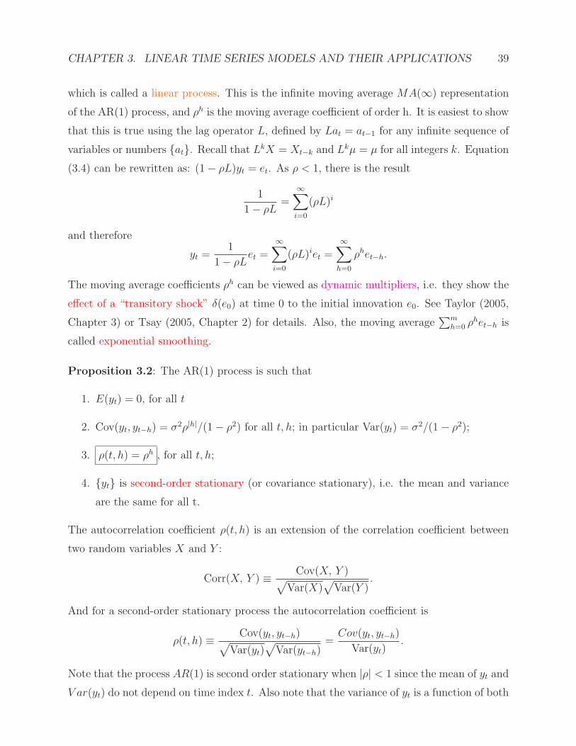
CHAPTER 3. LINEAR TIME SERIES MODELS AND THEIR APPLICATIONS 39
which is called a linear process. This is the infinite moving average MA(∞) representation
of the AR(1) process, and ρh is the moving average coefficient of order h. It is easiest to show
that this is true using the lag operator L, defined by Lat = at−1 for any infinite sequence of
variables or numbers at. Recall that LkX = Xt−k and Lkµ = µ for all integers k. Equation
(3.4) can be rewritten as: (1− ρL)yt = et. As ρ < 1, there is the result
1
1− ρL=
∞∑
i=0
(ρL)i
and therefore
yt =1
1− ρLet =
∞∑
i=0
(ρL)iet =∞∑
h=0
ρhet−h.
The moving average coefficients ρh can be viewed as dynamic multipliers, i.e. they show the
effect of a “transitory shock” δ(e0) at time 0 to the initial innovation e0. See Taylor (2005,
Chapter 3) or Tsay (2005, Chapter 2) for details. Also, the moving average∑m
h=0 ρhet−h is
called exponential smoothing.
Proposition 3.2: The AR(1) process is such that
1. E(yt) = 0, for all t
2. Cov(yt, yt−h) = σ2ρ|h|/(1− ρ2) for all t, h; in particular Var(yt) = σ2/(1− ρ2);
3. ρ(t, h) = ρh , for all t, h;
4. yt is second-order stationary (or covariance stationary), i.e. the mean and variance
are the same for all t.
The autocorrelation coefficient ρ(t, h) is an extension of the correlation coefficient between
two random variables X and Y :
Corr(X, Y ) ≡ Cov(X, Y )√Var(X)
√Var(Y )
.
And for a second-order stationary process the autocorrelation coefficient is
ρ(t, h) ≡ Cov(yt, yt−h)√Var(yt)
√Var(yt−h)
=Cov(yt, yt−h)
Var(yt).
Note that the process AR(1) is second order stationary when |ρ| < 1 since the mean of yt and
V ar(yt) do not depend on time index t. Also note that the variance of yt is a function of both
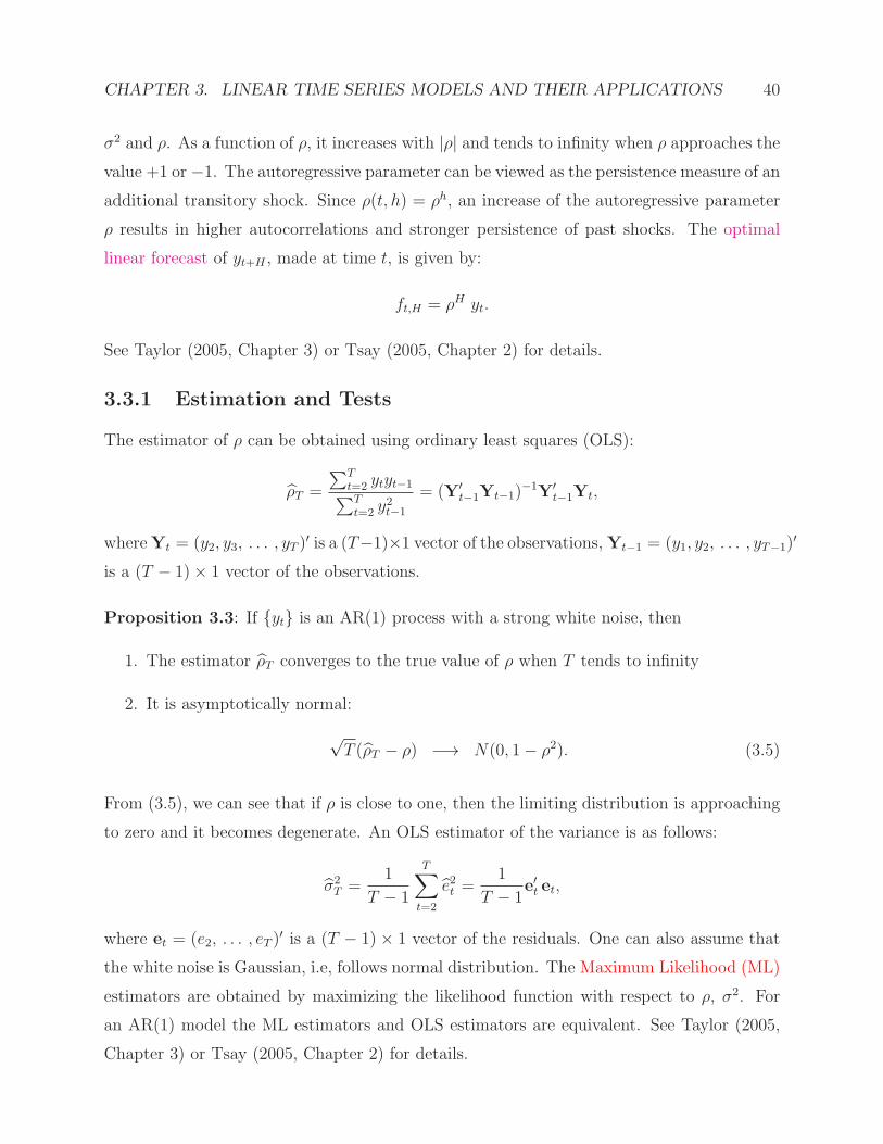
CHAPTER 3. LINEAR TIME SERIES MODELS AND THEIR APPLICATIONS 40
σ2 and ρ. As a function of ρ, it increases with |ρ| and tends to infinity when ρ approaches the
value +1 or −1. The autoregressive parameter can be viewed as the persistence measure of an
additional transitory shock. Since ρ(t, h) = ρh, an increase of the autoregressive parameter
ρ results in higher autocorrelations and stronger persistence of past shocks. The optimal
linear forecast of yt+H , made at time t, is given by:
ft,H = ρH yt.
See Taylor (2005, Chapter 3) or Tsay (2005, Chapter 2) for details.
3.3.1 Estimation and Tests
The estimator of ρ can be obtained using ordinary least squares (OLS):
ρT =
∑Tt=2 ytyt−1∑Tt=2 y
2t−1
= (Y′t−1Yt−1)
−1Y′t−1Yt,
whereYt = (y2, y3, . . . , yT )′ is a (T−1)×1 vector of the observations,Yt−1 = (y1, y2, . . . , yT−1)
′
is a (T − 1)× 1 vector of the observations.
Proposition 3.3: If yt is an AR(1) process with a strong white noise, then
1. The estimator ρT converges to the true value of ρ when T tends to infinity
2. It is asymptotically normal:
√T (ρT − ρ) −→ N(0, 1− ρ2). (3.5)
From (3.5), we can see that if ρ is close to one, then the limiting distribution is approaching
to zero and it becomes degenerate. An OLS estimator of the variance is as follows:
σ2T =
1
T − 1
T∑
t=2
e2t =1
T − 1e′t et,
where et = (e2, . . . , eT )′ is a (T − 1) × 1 vector of the residuals. One can also assume that
the white noise is Gaussian, i.e, follows normal distribution. The Maximum Likelihood (ML)
estimators are obtained by maximizing the likelihood function with respect to ρ, σ2. For
an AR(1) model the ML estimators and OLS estimators are equivalent. See Taylor (2005,
Chapter 3) or Tsay (2005, Chapter 2) for details.
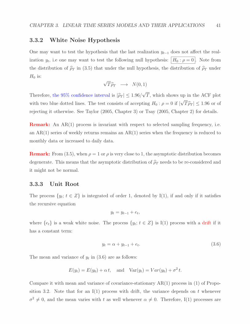
CHAPTER 3. LINEAR TIME SERIES MODELS AND THEIR APPLICATIONS 41
3.3.2 White Noise Hypothesis
One may want to test the hypothesis that the last realization yt−1 does not affect the real-
ization yt, i.e one may want to test the following null hypothesis: H0 : ρ = 0 . Note from
the distribution of ρT in (3.5) that under the null hypothesis, the distribution of ρT under
H0 is:√T ρT −→ N(0, 1)
Therefore, the 95% confidence interval is |ρT | ≤ 1.96/√T , which shows up in the ACF plot
with two blue dotted lines. The test consists of accepting H0 : ρ = 0 if |√T ρT | ≤ 1.96 or of
rejecting it otherwise. See Taylor (2005, Chapter 3) or Tsay (2005, Chapter 2) for details.
Remark: An AR(1) process is invariant with respect to selected sampling frequency, i.e.
an AR(1) series of weekly returns remains an AR(1) series when the frequency is reduced to
monthly data or increased to daily data.
Remark: From (3.5), when ρ = 1 or ρ is very close to 1, the asymptotic distribution becomes
degenerate. This means that the asymptotic distribution of ρT needs to be re-considered and
it might not be normal.
3.3.3 Unit Root
The process yt; t ∈ Z is integrated of order 1, denoted by I(1), if and only if it satisfies
the recursive equation
yt = yt−1 + et,
where et is a weak white noise. The process yt; t ∈ Z is I(1) process with a drift if it
has a constant term:
yt = α + yt−1 + et. (3.6)
The mean and variance of yt in (3.6) are as follows:
E(yt) = E(y0) + α t, and Var(yt) = V ar(y0) + σ2 t.
Compare it with mean and variance of covariance-stationary AR(1) process in (1) of Propo-
sition 3.2. Note that for an I(1) process with drift, the variance depends on t whenever
σ2 6= 0, and the mean varies with t as well whenever α 6= 0. Therefore, I(1) processes are

CHAPTER 3. LINEAR TIME SERIES MODELS AND THEIR APPLICATIONS 42
non-stationary. See Hamilton (1994, Chapter 17), Taylor (2005, Chapter 3), and Tsay (2005)
for details.
3.3.4 Estimation and Tests in the Presence of a Unit Root
The I(1) specification can be represented by a regression model:
yt = ρyt−1 + et, without drift (3.7)
yt = α + ρyt−1 + et, with drift (3.8)
and corresponds to the case when ρ = 1. The OLS estimators of the parameters α and ρ in
(3.7) and (3.8) can still be found but their properties are different from the standard case
when |ρ| < 1.
Proposition 3.4: If yt is an I(1) process without drift, OLS estimate of ρ, ρT , tends
asymptotically to 1.
Proposition 3.5: If yt is an I(1) process with drift, OLS estimate of ρ, ρT , tends asymp-
totically to 1 and αT to α.
Proposition 3.6: The ACF of a non-stationary time series decays very slowly as a function
of lag h. The PACF of a non-stationary time series tends to have a peak very near unity at
lag 1, with other values less than the significance level. Indeed, if h > 0,
ρ(yt, yt+h) =
√t
t+ h,
which depends on t.
The starting point for the Dickey-Fuller (DF) test is the autoregressive model of order one,
AR(1) as in (3.8). If ρ = 1, yt is nonstationary and contains a stochastic trend. Therefore,
within the AR(1) model, the hypothesis that yt has a trend can be tested by testing:
H0 : ρ = 1 vs. H1 : ρ < 1.
This test is most easily implemented by estimating a modified version of (3.8). Subtract yt−1
from both sides and let δ = ρ− 1. Then, model (3.8) becomes:
∆ yt = α + δyt−1 + et (3.9)
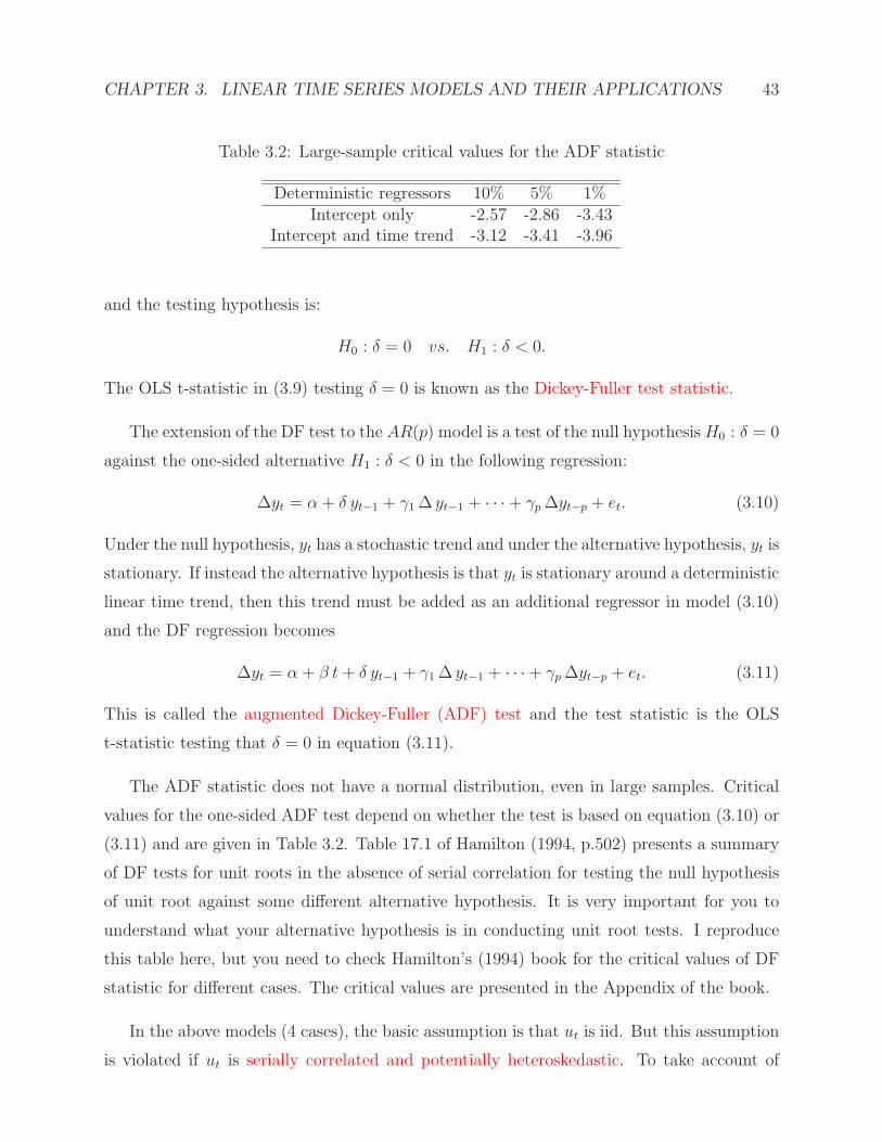
CHAPTER 3. LINEAR TIME SERIES MODELS AND THEIR APPLICATIONS 43
Table 3.2: Large-sample critical values for the ADF statistic
Deterministic regressors 10% 5% 1%Intercept only -2.57 -2.86 -3.43
Intercept and time trend -3.12 -3.41 -3.96
and the testing hypothesis is:
H0 : δ = 0 vs. H1 : δ < 0.
The OLS t-statistic in (3.9) testing δ = 0 is known as the Dickey-Fuller test statistic.
The extension of the DF test to the AR(p) model is a test of the null hypothesisH0 : δ = 0
against the one-sided alternative H1 : δ < 0 in the following regression:
∆yt = α + δ yt−1 + γ1 ∆ yt−1 + · · ·+ γp ∆yt−p + et. (3.10)
Under the null hypothesis, yt has a stochastic trend and under the alternative hypothesis, yt is
stationary. If instead the alternative hypothesis is that yt is stationary around a deterministic
linear time trend, then this trend must be added as an additional regressor in model (3.10)
and the DF regression becomes
∆yt = α + β t+ δ yt−1 + γ1 ∆ yt−1 + · · ·+ γp ∆yt−p + et. (3.11)
This is called the augmented Dickey-Fuller (ADF) test and the test statistic is the OLS
t-statistic testing that δ = 0 in equation (3.11).
The ADF statistic does not have a normal distribution, even in large samples. Critical
values for the one-sided ADF test depend on whether the test is based on equation (3.10) or
(3.11) and are given in Table 3.2. Table 17.1 of Hamilton (1994, p.502) presents a summary
of DF tests for unit roots in the absence of serial correlation for testing the null hypothesis
of unit root against some different alternative hypothesis. It is very important for you to
understand what your alternative hypothesis is in conducting unit root tests. I reproduce
this table here, but you need to check Hamilton’s (1994) book for the critical values of DF
statistic for different cases. The critical values are presented in the Appendix of the book.
In the above models (4 cases), the basic assumption is that ut is iid. But this assumption
is violated if ut is serially correlated and potentially heteroskedastic. To take account of
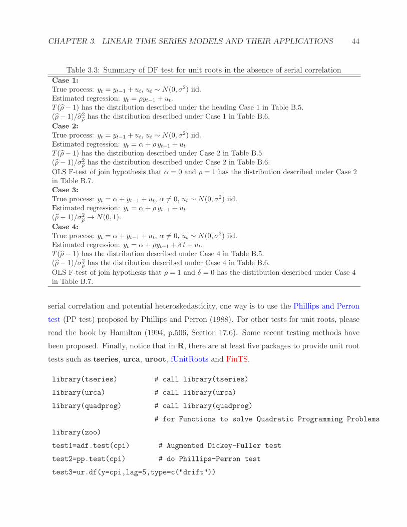
CHAPTER 3. LINEAR TIME SERIES MODELS AND THEIR APPLICATIONS 44
Table 3.3: Summary of DF test for unit roots in the absence of serial correlation
Case 1:
True process: yt = yt−1 + ut, ut ∼ N(0, σ2) iid.Estimated regression: yt = ρyt−1 + ut.T (ρ− 1) has the distribution described under the heading Case 1 in Table B.5.(ρ− 1)/σ2
ρ has the distribution described under Case 1 in Table B.6.
Case 2:
True process: yt = yt−1 + ut, ut ∼ N(0, σ2) iid.Estimated regression: yt = α+ ρ yt−1 + ut.T (ρ− 1) has the distribution described under Case 2 in Table B.5.(ρ− 1)/σ2
ρ has the distribution described under Case 2 in Table B.6.
OLS F-test of join hypothesis that α = 0 and ρ = 1 has the distribution described under Case 2in Table B.7.Case 3:
True process: yt = α+ yt−1 + ut, α 6= 0, ut ∼ N(0, σ2) iid.Estimated regression: yt = α+ ρ yt−1 + ut.(ρ− 1)/σ2
ρ → N(0, 1).
Case 4:
True process: yt = α+ yt−1 + ut, α 6= 0, ut ∼ N(0, σ2) iid.Estimated regression: yt = α+ ρyt−1 + δ t+ ut.T (ρ− 1) has the distribution described under Case 4 in Table B.5.(ρ− 1)/σ2
ρ has the distribution described under Case 4 in Table B.6.
OLS F-test of join hypothesis that ρ = 1 and δ = 0 has the distribution described under Case 4in Table B.7.
serial correlation and potential heteroskedasticity, one way is to use the Phillips and Perron
test (PP test) proposed by Phillips and Perron (1988). For other tests for unit roots, please
read the book by Hamilton (1994, p.506, Section 17.6). Some recent testing methods have
been proposed. Finally, notice that in R, there are at least five packages to provide unit root
tests such as tseries, urca, uroot, fUnitRoots and FinTS.
library(tseries) # call library(tseries)
library(urca) # call library(urca)
library(quadprog) # call library(quadprog)
# for Functions to solve Quadratic Programming Problems
library(zoo)
test1=adf.test(cpi) # Augmented Dickey-Fuller test
test2=pp.test(cpi) # do Phillips-Perron test
test3=ur.df(y=cpi,lag=5,type=c("drift"))
CHAPTER 3. LINEAR TIME SERIES MODELS AND THEIR APPLICATIONS 45
See Hamilton (1994, Chapter 17), Taylor (2005, Chapter 3), and Tsay (2005, Chapter 2)
for details.
3.4 MA(1) Model
The moving average process of order one, denoted MA(1), is defined as:
yt = α + et + θet−1.
It is assumed that moving-average parameter θ satisfies the invertibility condition |θ| < 1 and
then the optimal linear forecasts can be calculated. An MA(1) process has autocorrelations
ρ1 =θ
1 + θ2, ρτ = 0 for τ ≥ 2.
The optimal linear forecasts are given by
ft,1 = α + θ(yt − ft−1,1), and ft,H = α, H ≥ 2.
See Hamilton (1994, Chapter 4), Taylor (2005, Chapter 3), and Tsay (2005, Chapter 2) for
details.
3.5 ARMA, ARIMA, and ARFIMA Processes
According to the Wold theorem, any second-order stationary time process can be written as
a moving average of order infinity. See Hamilton (1994, Chapter 4), Taylor (2005, Chapter
3), and Tsay (2005, Chapter 2) for details.
3.5.1 ARMA(1,1) Process
Consider a combination of the AR(1) process and MA(1) models defined by
yt = φyt−1 + et + θet−1,
which is called the autoregressive, moving-average process, denoted ARMA(1,1). It is as-
sumed that 0 < |φ| < 1 and 0 < θ < 1. Autocorrelations are given by
ρτ = A(φ, θ)φτ , τ ≥ 1
with
A(φ, θ) =(1 + φθ)(φ+ θ)
φ(1 + 2φθ + θ2).
CHAPTER 3. LINEAR TIME SERIES MODELS AND THEIR APPLICATIONS 46
The ARMA(1,1) process can be written using the lag operator as:
(1− φL)yt = (1 + θL)et.
This implies that
yt =1 + θL
1− φLet =
( ∞∑
i=0
φiLi
)(1 + θL)et = et + (φ+ θ)
∞∑
i=1
φi−1et−i,
i.e. the ARMA(1,1) process can be written as MA(∞) process. The optimal linear forecast
of yt+1 is
ft,1 = (φ+ θ)∞∑
i=1
(−θ)i−1yt+1−i
or
ft,1 = (φ+ θ)yt − θft−1,1.
To forecast observed values, we replace the parameters α, φ, and θ by their estimates. The
optimal linear forecast further ahead is constructed as follows:
ft,H = φH ft,1.
3.5.2 ARMA(p,q) Process
A second-order stationary (covariance-stationary) process yt is an ARMA(p,q) process of
autoregressive order p and moving average order q if it can be written as
yt = φ1yt−1 + . . . + φpyt−p + et − θ1et−1 − . . . − θqet−q,
where φp 6= 0, θq 6= 0 and et is a weak white noise. The ARMA process can be written as
Φ(L)yt = Θ(L)et, (3.12)
where Φ(L) = 1− φ1L− φ2L2 − . . . − φpL
p and Θ(L) = 1 + θ1L+ θ2L2 + . . . + θ2L
q.
Now the question is how to select among various plausible models. Box, Jenkins, and
Reinsel (1994) described the Box-Jenkins methodology for selecting an appropriate ARMA
model. We mention that two criteria which reward reducing the squared error and penalize
for additional parameters are the Akaike Information Criterion
AIC(K) = log σ2 +2K
n
CHAPTER 3. LINEAR TIME SERIES MODELS AND THEIR APPLICATIONS 47
and the Schwarz Information Criterion
SIC(K) = log σ2 +K log(n)
n;
(Schwarz, 1978) where K is the number of parameters fitted (exclusive of variance parame-
ters) and σ2 is the maximum likelihood estimator for the variance. This is sometimes termed
the Bayesian Information Criterion, BIC and will often yield models with fewer parameters
than the other selection methods. A modification to AIC(K) that is particularly well suited
for small samples was suggested by Hurvich and Tsai (1989). This is the corrected AIC,
given by
AICC(K) = log σ2 +n+K
n−K + 2.
The rule for all three measures above is to choose the value of K leading to the smallest
value of AIC(K) or SIC(K) or AICC(K). See Brockwell and Davis (1991, Section 9.3) for
details. For more details about model selection methodologies, please read Chapter 2 of my
lecture notes (see Cai (2007, Chapter 2)).
The R commands for fitting and simulating an ARIMA model are
arima(x, order = c(0, 0, 0),seasonal = list(order = c(0, 0, 0), period = NA),
xreg = NULL, include.mean = TRUE, transform.pars = TRUE, fixed = NULL,
init = NULL, method = c("CSS-ML", "ML", "CSS"), n.cond,
optim.control = list(), kappa = 1e6)
arima.sim(model, n, rand.gen = rnorm, innov = rand.gen(n, ...),
n.start = NA, start.innov = rand.gen(n.start, ...), ...)
ar(x, aic = TRUE, order.max = NULL,
method=c("yule-walker", "burg", "ols", "mle", "yw"),
na.action, series, ...)
CHAPTER 3. LINEAR TIME SERIES MODELS AND THEIR APPLICATIONS 48
3.5.3 AR(p) Model
The series yt; t ∈ Z follows an autoregressive process of order p, denoted AR(p), if and
only if it can be written as
yt =
p∑
j=1
φjyt−j + et, (3.13)
where et, t ∈ Z is a weak white noise with variance Var(et) = σ2. It is convenient to
rewrite (3.13), using the back-shift operator, as
φ(L) yt = wt, where φ(L) = 1− φ1 L− φ2 L2 − · · · − φp L
p, (3.14)
is a polynomial with roots (solutions of φ(L) = 0) outside the unit circle (|Lj| > 1)1. The
restrictions are necessary for expressing the solution yt of (3.14) in terms of present and past
values of wt, which is called invertibility of an AR(p) series. That solution has the form
yt = ψ(L)wt, where ψ(L) =∞∑
k=0
ψk Lk, (3.15)
is an infinite polynomial (ψ0 = 1), with coefficients determined by equating coefficients of B
in
ψ(L)φ(L) = 1. (3.16)
Equation (3.15) can be obtained formally by noting that choosing ψ(L) satisfying (3.16),
and multiplying both sides of (3.15) by ψ(L) gives the representation (3.15). It is clear that
the random walk has φ1 = 1 and φk = 0 for all k ≥ 2, which does not satisfy the restriction
and the process is nonstationary. yt is stationary if∑
k |ψk| < ∞; see Proposition 3.1.2 in
Brockwell and Davis (1991, p.84), which can be weakened by∑
k ψ2k < ∞; see Hamilton
(1994, p.52).
Question: How to identify the order p in an AR(p) model intuitively?
Proposition 3.7 The partial autocorrelation function (PACF) as a function of lag h is zero
for h > p, the order of the autoregressive process. This enables one to make a prelimi-
nary identification of the order p of the process using the partial autocorrelation function
PACF. Simply choose the order beyond which most of the sample values of the PACF are
approximately zero.
1This restriction is a sufficient and necessary condition for an ARMA time series to be invertible; seeSection 3.7 in Hamilton (1994) or Theorem 3.1.2 in Brockwell and Davis (1991, p.86) and the relateddiscussions.

CHAPTER 3. LINEAR TIME SERIES MODELS AND THEIR APPLICATIONS 49
To verify the above, note that the PACF is basically the last coefficient obtained when
minimizing the squared error
MSE = E
(yt+h −
h∑
k=1
ak yt+h−k
)2 .
Setting the derivatives with respect to aj equal to zero leads to the equations
E
(yt+h −
h∑
k=1
ak yt+h−k
)2
yt+h−j
= 0
This can be written as
ρy(j)−h∑
k=1
ak ρy(j − k) = 0
for 1 ≤ j ≤ h. Now, it is clear that, for an AR(p), we may take ak = φk for k ≤ p and ak = 0
for k > p to get a solution for the above equation. This implies Proposition 3.7 above.
To estimate the coefficients of the pth order AR in (3.13), write the equation (3.14) as
yt −p∑
k=1
φk yt−k = wt
and multiply both sides by yt−h for any h ≥ 1. Assuming that the mean E(yt) = 0, and
using the definition of the autocovariance function leads to the equation
E
[(yt yt−h −
p∑
k=1
φk yt−k yt−h
]= E[wt yt−h].
The left-hand side immediately becomes ρy(h)−∑p
k=1 φk ρy(h−k). The representation (3.15)
implies that
E[wt yt−h] = E[wt(wt−h + φ1wt−h−1 + φ2wt−h−2 + · · ·)] =σ2w, if h = 0,
0 otherwise.
Hence, we may write the equations for determining γx(h) as
ρy(0)−p∑
k=1
φk ρy(−k) = σ2w (3.17)
and
ρy(h)−p∑
k=1
φk ρy(h− k) = 0 for h ≥ 1. (3.18)
CHAPTER 3. LINEAR TIME SERIES MODELS AND THEIR APPLICATIONS 50
Note that one will need the property ρy(h) = ρy(−h) in solving these equations. Equations
(3.17) and (3.18) are called the Yule-Walker Equations (see Yule, 1927, Walker, 1931).
Having decided on the order p of the model, it is clear that, for the estimation step, one
may write the model (3.13) in the regression form
yt = φ′zt + wt, (3.19)
where φ = (φ1, φ2, · · · , φp)′ corresponds to β and zt = (yt−1, yt−2, · · · , yt−p)
′ is the vector
of dependent variables. Taking into account the fact that yt is not observed for t ≤ 0, we
may run the regression approach for t = p+1, · · · , n to get estimators for φ and for σ2, the
variance of the white noise process. These so-called conditional maximum likelihood
estimators are commonly used because the exact maximum likelihood estimators involve
solving nonlinear equations; see Chapter 5 in Hamilton (1994) for details and we will discuss
this issue later.
3.5.4 MA(q)
We may also consider processes that contain linear combinations of underlying unobserved
shocks, say, represented by white noise series wt. These moving average components generate
a series of the form
yt = wt −q∑
k=1
θk wt−k, (3.20)
where q denotes the order of the moving average component and θk(1 ≤ k ≤ q) are param-
eters to be estimated. Using the back-shift notation, the above equation can be written in
the form
yt = θ(L)wt with θ(L) = 1−q∑
k=1
θk Lk, (3.21)
where θ(L) is another polynomial in the shift operator L. It should be noted that the MA
process of order q is a linear process of the form considered earlier with ψ0 = 1, ψ1 = −θ1,· · ·, ψq = −θq. This implies that the ACF will be zero for lags larger than q because terms
in the form of the covariance function will all be zero. Specifically, the exact forms are
ρy(0) = σ2w
(1 +
q∑
k=1
θ2k
)and ρy(h) = σ2
w
(−θh +
q−h∑
k=1
θk+hθk
)(3.22)
for 1 ≤ h ≤ q − 1, with ρy(q) = −σ2w θq, and ρx(h) = 0 for h > q. Hence, we will have the
property of ACF for for MA Series.
CHAPTER 3. LINEAR TIME SERIES MODELS AND THEIR APPLICATIONS 51
Property 3.8: For a moving average series of order q, note that the autocorrelation function
(ACF) is zero for lags h > q, i.e. ρy(h) = 0 for h > q. Such a result enables us to diagnose
the order of a moving average component by examining ρy(h) and choosing q as the value
beyond which the coefficients are essentially zero.
Fitting the pure moving average term turns into a nonlinear problem as we can see by
noting that either maximum likelihood or regression involves solving (3.20) or (3.21) for wt,
and minimizing the sum of the squared errors. Suppose that the roots of π(L) = 0 are all
outside the unit circle, then this is possible by solving π(L) θ(L) = 1, so that, for the vector
parameter θ = (θ1, · · · , θq)′, we may write
wt(θ) = π(L) yt (3.23)
and minimize SSE(θ) =∑n
t=q+1w2t (θ) as a function of the vector parameter θ. We do not
really need to find the operator π(L) but can simply solve (3.23) recursively for wt, with
w1, w2, · · · , wq = 0, and wt(θ) = yt +∑q
k=1 θk wt−k for q + 1 ≤ t ≤ n. It is easy to verify
that SSE(θ) will be a nonlinear function of θ1, θ2, · · · , θq. However, note that by the Taylor
expansion
wt(θ) ≈ wt(θ0) +
(∂wt(θ)
∂θ0
)(θ − θ0),
where the derivative is evaluated at the previous guess θ0. Rearranging the above equation
leads to
wt(θ0) ≈(−∂wt(θ)
∂θ0
)(θ − θ0) + wt(θ),
which is just a regression model. Hence, we can begin with an initial guess θ0 = (0.1, 0.1, · · · , 0.1)′,say and successively minimize SSE(θ) until convergence. See Chapter 5 in Hamilton (1994)
for details and we will discuss this issue later.
Forecasting: In order to forecast a moving average series, note that yt+h = wt+h −∑q
k=1 θk wt+h−k. The results below (3.28) imply that ytt+h = 0 if h > q and if h ≤ q,
ytt+h = −q∑
k=h
θk wt+h−k,
where the wt values needed for the above are computed recursively as before. Because of
(3.15), it is clear that ψ0 = 1 and ψk = −θk for 1 ≤ k ≤ q and these values can be substituted
directly into the variance formula (3.31). That is, P tt+h = σ2
w
(1 +
∑h−1k=1 θ
2k
).

CHAPTER 3. LINEAR TIME SERIES MODELS AND THEIR APPLICATIONS 52
3.5.5 AR(∞) Process
Under the condition that the roots of the moving average polynomial Θ(z) lie outside the
unit circle, (3.12) can be rewritten as:
Φ(L)
Θ(L)yt = et, or B(L)yt = et, or
∞∑
h=0
bhyt−h = et,
where b1, b2, . . . are appropriately defined functions of φ’s and θ’s.
3.5.6 MA(∞) Process
Under the condition that the roots of the autoregressive polynomial Φ(z) lie outside the unit
circle, we can rewrite (3.12) as:
yt =Θ(L)
Φ(L)et = A(L)et =
∞∑
h=0
ahet−h,
where A(L) = Θ(L)Φ(L)−1 = 1 + a1L + a2L2 + . . . and the parameters a1, a2, . . . are
appropriately defined functions of φ’s and θ’s. This model is also called a linear process in
the stochastic processes literature.
3.5.7 ARIMA Processes
The acronym ARIMA(p,1,q) is used for a process yt, when it is non-stationary but its
first differences, yt − yt−1, follow a stationary ARMA(p,q) process. The additional letter
“I” states that the process yt is integrated, while the numeral “1” indicates that only one
application of differences is required to achieve stationarity.
3.5.8 ARFIMA Process
An ARMA(p,q) process can be described as
φ(L)yt = θ(L)et.
The ARFIMA(p,d,q) process can be written as
(1− L)dφ(L)yt = θ(L)et, or yt = (1− L)−dφ(L)−1θ(L)et
This ARFIMA process is stationary when d < 0.5. Assuming that d is positive, it is a special
case of a long memory process or a fractional process or long range dependent time series.
CHAPTER 3. LINEAR TIME SERIES MODELS AND THEIR APPLICATIONS 53
The letter d means that the process yt is fractional with the index d, which is called
the long memory parameter or H = d + 1/2 is called the Hurst parameter; see Hurst
(1951). This is a very big area and there are a lot research activities in this area. A long
memory process has widely used in financial applications such as modeling the relationship
between the implied and realized volatilities; see the survey paper by Andersen, Bollerslev,
Christoffersen and Diebold (2005).
Long memory time series have been a popular area of research in economics, finance and
statistics and other applied fields such as hydrological sciences during the recent years. Long
memory dependence was first observed by the hydrologist Hurst (1951) when analyzing the
minimal water flow of the Nile River when planning the Aswan Dam. Granger (1966) gave
an intensive discussion about the application of long memory dependence in economics and
its consequence was initiated. Here we only briefly discuss some most useful time series
models in the literature. For more details about the aforementioned models, please read the
books by Brockwell and Davis (1991) and Hamilton (1994).
Exercises: Please use Monte Carlo simulation method to generate data from the above
models and make graphs to what you can make conclusions from the graphs.
Applications
The usage of the function fracdiff() is
fracdiff(x, nar = 0, nma = 0,
ar = rep(NA, max(nar, 1)), ma = rep(NA, max(nma, 1)),
dtol = NULL, drange = c(0, 0.5), h, M = 100)
This function can be used to compute the maximum likelihood estimators of the parameters
of a fractionally-differenced ARIMA(p, d, q) model, together (if possible) with their estimated
covariance and correlation matrices and standard errors, as well as the value of the maximized
likelihood. The likelihood is approximated using the fast and accurate method of Haslett
and Raftery (1989). To generate simulated long-memory time series data from the fractional
ARIMA(p, d, q) model, we can use the following function fracdiff.sim() and its usage is
fracdiff.sim(n, ar = NULL, ma = NULL, d,
rand.gen = rnorm, innov = rand.gen(n+q, ...),
CHAPTER 3. LINEAR TIME SERIES MODELS AND THEIR APPLICATIONS 54
n.start = NA, allow.0.nstart = FALSE, ..., mu = 0.)
An alternative way to simulate a long memory time series is to use the function arima.sim().
The menu for the package fracdiff can be downloaded from the web site at
http://cran.cnr.berkeley.edu/doc/packages/fracdiff.pdf
The function spec.pgram() in R calculates the periodogram using a fast Fourier trans-
form, and optionally smooths the result with a series of modified Daniell smoothers (moving
averages giving half weight to the end values). The usage of this function is
spec.pgram(x, spans = NULL, kernel, taper = 0.1,
pad = 0, fast = TRUE, demean = FALSE, detrend = TRUE,
plot = TRUE, na.action = na.fail, ...)
We can also use the function spectrum() to estimate the spectral density of a time series
and its usage is
spectrum(x, ..., method = c("pgram", "ar"))
Finally, it is worth to pointing out that there is a package called longmemo for long-memory
processes, which can be downloaded from
http://cran.cnr.berkeley.edu/doc/packages/longmemo.pdf. This package also pro-
vides a simple periodogram estimation by function per() and other functions like llplot()
and lxplot() for making graphs for spectral density. See the menu for details.
Example: As an illustration, Figure 3.4 show the sample ACFs of the absolute series
of daily simple returns for the CRSP value-weighted (left top panel) and equal-weighted
(right top panel) indexes from July 3, 1962 to December 31, 1997 and the sample partial
autocorrelation function of the absolute series of daily simple returns for the CRSP value-
weighted (left middle panel) and equal-weighted (right middle panel) indexes. The ACFs
are relatively small in magnitude, but decay very slowly; they appear to be significant at
the 5% level even after 300 lags. There are only the first few lags for PACFs outside the
confidence interval and then the rest is basically within the confidence interval. For more
information about the behavior of sample ACF of absolute return series, see Ding, Granger,
and Engle (1993). To estimate the long memory parameter estimate d, we can use the
function fracdiff() in the package fracdiff in R and results are d = 0.1867 for the absolute

CHAPTER 3. LINEAR TIME SERIES MODELS AND THEIR APPLICATIONS 55
0 100 200 300 400−0.1
0.0
0.1
0.2
0.3
0.4
ACF for value−weighted index
0 100 200 300 400−0.1
0.0
0.1
0.2
0.3
0.4
ACF for equal−weighted index
0 100 200 300 400−0.1
0.0
0.1
0.2
0.3
PACF for value−weighted index
0 100 200 300 400−0.1
0.0
0.1
0.2
0.3
PACF for equal−weighted index
0.00 0.01 0.02 0.03 0.04 0.05 0.06 0.07
−11
−9−8
−7−6
Log Smoothed Spectral Density of VW
0.00 0.01 0.02 0.03 0.04 0.05 0.06 0.07
−12
−10
−8−6
Log Smoothed Spectral Density of EW
Figure 3.4: Sample autocorrelation function of the absolute series of daily simple returnsfor the CRSP value-weighted (left top panel) and equal-weighted (right top panel) indexes.Sample partial autocorrelation function of the absolute series of daily simple returns for theCRSP value-weighted (left middle panel) and equal-weighted (right middle panel) indexes.The log smoothed spectral density estimation of the absolute series of daily simple returnsfor the CRSP value-weighted (left bottom panel) and equal-weighted (right bottom panel)indexes.
returns of the value-weighted index and d = 0.2732 for the absolute returns of the equal-
weighted index. To support our conclusion above, we plot the log smoothed spectral density
estimation of the absolute series of daily simple returns for the CRSP value-weighted (left
bottom panel) and equal-weighted (right bottom panel). They show clearly that both log
spectral densities decay like a log function and they support the spectral densities behavior.
CHAPTER 3. LINEAR TIME SERIES MODELS AND THEIR APPLICATIONS 56
3.6 R Commands
Classical time series functionality in R is provided by the arima() and KalmanLike() com-
mands in the basic R distribution. The dse packages provides a variety of more advanced
estimation methods; fracdiff can estimate fractionally integrated series; longmemo cov-
ers related material. For volatily modeling, the standard GARCH(1,1) model can be es-
timated with the garch() function in the tseries package. Unit root and cointegration
tests are provided by tseries, urca and uroot. The Rmetrics bundle comprised of the
fArma, fAsianOptions, fAssets, fBasics, fBonds, fCalendar, fCopulae, fEcofin, fExoticOp-
tions, fExtremes, fGarch, fImport, fMultivar, fNonlinear, fOptions, fPortfolio, fRegression,
fSeries, fTrading, fUnitRoots and fUtilities packages contains a very large number of relevant
functions for different aspect of empirical and computational finance, including a number
of estimation functions for ARMA, GARCH, long memory models, unit roots and more.
The ArDec implements autoregressive time series decomposition in a Bayesian framework.
The dyn and dynlm are suitable for dynamic (linear) regression models. Several pack-
ages provide wavelet analysis functionality: rwt, wavelets, waveslim, wavethresh. Some
methods from chaos theory are provided by the package tseriesChaos. For more details,
please see the file in the web site at http://www.math.uncc.edu/˜ zcai/CRAN-Finance.html
or http://cran.cnr.berkeley.edu/src/contrib/Views/Finance.html which is downloadable.
3.7 Regression Models With Correlated Errors
See my lecture notes on ”Advanced Topics in Analysis of Economic and Financial Data Using
R and SAS”, which can be downloaded from http://www.math.uncc.edu/˜ zcai/cai-notes.pdf
3.8 Comments on Nonlinear Models and Their Appli-
cations
All aforementioned models are basically linear but we have not touched with nonlinear time
series models. It requires much deeper statistics knowledge for nonlinear time series models.
Indeed, during the last two decades, there have been a lot of research activities on nonlinear
models and their applications, particularly, in finance; see Tsay (2005, Chapter 4) and Fan
and Yao (2003). Also, see Chapter 12 of Gourieroux and Jasiak (2001) and Chapter 16 of
Taylor (2005) for nonlinear models in finance.
CHAPTER 3. LINEAR TIME SERIES MODELS AND THEIR APPLICATIONS 57
3.9 Problems
3.9.1 Problems
1. Download weekly (daily) price data for any stock or index, for example, Microsoft
(MSFT) stock (Pt) for 03/13/86 - 1/15/2008. It is okey if you download other stocks
and indices.
(a) Compute mean (µ), standard deviation (σ), skewness (Sk), and kurtosis (Kr)
for Microsoft stock returns. Comment your findings on skewness and kurtosis of
Microsoft stock returns. Are your results as expected?
# Mean, Variance:
rt=rnorm(100)
mean(rt)
var(rt)
# Skewness, Kurtosis:
library(fUtilities) # call library -- fUtilities
skewness(rt)
kurtosis(rt)
(b) Use constant expected returns (CER) model to simulate a sample of “artificial
data”:
rt = µ+ et, 1 ≤ t ≤ T, et ∼ N(0, σ2)
In generation of the artificial sample, set µ equal to the sample mean of Microsoft
returns and σ2 equal to the sample variance of Microsoft returns, i.e. µ = µ,
σ2 = σ2. Use the R random number generator to generate error terms et for
1 ≤ t ≤ T for different values of T . Generate the artificial sample of returns and
prices using the above model. For generating prices, set p0 = 1.
(c) If the CER model is a good model to describe stock market returns, then the
simulated (artificial) sample of returns should have the same properties (mean,
variance, skewness, kurtosis, persistence) as the sample Microsoft stock market
returns.
(i) Compare the mean from the simulated sample and the sample mean of
Microsoft returns.

CHAPTER 3. LINEAR TIME SERIES MODELS AND THEIR APPLICATIONS 58
(ii) Compare the variance from the simulated sample and the sample variance
of Microsoft returns.
(iii) Compare the skewness from the simulated sample and the sample skew-
ness of Microsoft returns.
(iv) Compare the kurtosis from the simulated sample and the sample kur-
tosis of Microsoft returns.
(v) Can CER model explain excess kurtosis of stock returns?
What you need is to simulate 1000 times for the given sample
size. For each sample, compute sample mean, sample variance,
sample skewness, and sample kurtosis and then compute the
median of each of them as estimated mean, variance, skewness
and kurtosis from the simulated model. Finally compare the
estimated values from the simulated model with the true values
from the real data.
2. Estimate the CER model for Microsoft using the OLS estimation.
(a) Use t-statistic to test the null hypothesis that the mean of Microsoft returns is
zero.
(b) Look at the coefficient of determination R2. What can you say about the fit of
the CER model for Microsoft returns?
fit=lm(rt~1) # fit a constant term of regression model
print(summary(fit)) # print the results on the screen
(c) Use CER model to form the forecast for rT+1 given all the information up to
period T , i.e. rT+1 |T .
(d) Use CER model to form the forecast rT+2|T .
Please think about how to do a forecasting for a CER model.
3. Estimate the AR(1) process of the following form for Microsoft stock returns:
rt = ρ rt−1 + et, t = 1, . . . , T.
(a) Estimate the model using OLS.

CHAPTER 3. LINEAR TIME SERIES MODELS AND THEIR APPLICATIONS 59
(b) Use both t-statistic based on the OLS estimate ρ and ADF test to test the hy-
pothesis of unit root for this model.
(c) Test the null hypothesis that ρ is zero.
(d) Look at the coefficient of determination R2. What can you say about the fit of
the AR(1) model without drift for Microsoft returns?
n=length(r) # rt the series for some return
y1<-rt[2:n]
x1<-rt[1:(n-1)]
fit=lm(y1~-1+x1) # fit an AR(1) model without intercept
# Alternatively, you can use the command ar() to fit AR(p) using
fit1=ar(rt) # Let AIC select automatically the best model
print(summary(fit)) # print the results on the screen
(e) Use AR(1) model without drift to form the forecast rT+1|T . Write down the
formula.
(f) Use AR(1) model without drift to form the forecast rT+2|T . Write down the
formula.
See Section 3.9.2 for R codes for predictions.
4. Estimate the AR(1) process with drift for Microsoft stock returns:
rt = µ+ ρ rt−1 + et, 1 ≤ t ≤ T.
(a) Estimate the model using OLS.
(b) Use both t-statistic based on the OLS estimate ρ and the ADF test to test the
hypothesis of unit root for this model.
(c) Find the estimate of the first autocorrelation coefficient of the error term (you
need to use residual et = rt − µ − ρ rt−1). Test the null hypothesis that this
coefficients of et are zero.
(d) Look at the coefficient of determination R2. What can you say about the fit of
the AR(1) model with drift for Microsoft returns?
(e) Use AR(1) model without drift to form the forecast rT+1|T . Write down the
formula and make computations in R. For details, see Section 3.9.2.

CHAPTER 3. LINEAR TIME SERIES MODELS AND THEIR APPLICATIONS 60
(f) Use AR(1) model without drift to form the forecast rT+2|T . Write down the
formula and make computations in R. For details, see Section 3.9.2.
5. Estimate the AR(p) process with drift for Microsoft stock returns:
rt = µ+ φ1 rt−1 + · · ·+ φp rt−p + et, 1 ≤ t ≤ T.
(a) Estimate the model using OLS. Explain how you choose the lag length p.
(b) Test the null hypothesis that all autoregressive parameters are simultaneously
equal to zero, i.e. H0 : φ1 = · · · = φp = 0.
(c) Test the null hypothesis that µ = 0.
(d) What do these tests tell you about predictability of MSFT stock returns using
AR(p) model?
n=length(rt) # rt the series for some return
p<-??? # set up the number of lags
y1<-rt[(p+1):n]
xx<-rep(1,p*(n-p))
dim(xx)=c(n-p,p)
for(i in 1:p)
xx[,i]<-rt[i:(n-p+i-1)]
fit=lm(y1~xx)
# fit an AR(p) model with an intercept
3.9.2 R Code
Predictions
# 2-16-2008
graphics.off()
data=read.csv(file="c:/zcai/res-teach/econ6219/Bank-of-America.csv",header=T)
x=data[,5] # get the closing prices
x=rev(x) # reverse order of observations
n=length(x) # sample size
CHAPTER 3. LINEAR TIME SERIES MODELS AND THEIR APPLICATIONS 61
rt=diff(log(x)) # log return
n1=length(rt)
# do prediction
m=20 # leave the last m observations for prediction
# One-Step Ahead Forecasting
pred_1=rep(0,m)
for(i in 1:m)
fit1=arima0(rt[1:(n1-m+i-1)],order=c(1,0,0)) # fit an AR(1) model
pred0=predict(fit1,n.ahead=1)
pred_1[i]=pred0$pred[1] # compute predicted values
print(c("One-Step Ahead Forecasting"))
print(pred_1)
# Two-Step Ahead Forecasting
pred_2=rep(0,m)
for(i in 1:m)
fit1=arima0(rt[1:(n1-m+i-2)],order=c(1,0,0)) # fit an AR(1) model
pred0=predict(fit1,n.ahead=2) # two-step ahead forecasting
pred_2[i]=pred0$pred[2]
print(c("Two-Step Ahead Forecasting"))
print(pred_2)
3.10 Appendix A: Linear Forecasting
Assume that the records of an AR(1) process yt contain observations up to time T and we
wish to predict unknown future value yt+H that is H steps ahead. H is called the forecast
horizon.
Proposition 3.9: If yt is AR(1) process, the linear forecast at horizon H is
LE[yt+H |YT ] = ρH yT ,
CHAPTER 3. LINEAR TIME SERIES MODELS AND THEIR APPLICATIONS 62
while corresponding forecast error is
eT (H) = yt+H − ρH yt.
When the forecast horizon increases, the accuracy of forecast deteriorates. The relative
forecast accuracy can measured by the ratio:
1− Var(eT (H))
Var(yT+H)= ρ2H .
Since we use an estimate ρT in practice, the empirical forecast for H steps ahead is
yT+H = ρHT yT
and the associated prediction interval isyT+H ± 2σ2
T
[1− ρ2HT1− ρ2T
]1/2.
3.11 Appendix B: Forecasting Based on AR(p) Model
Time series analysis has proved to be fairly good way of producing forecasts. Its drawback
is that it is typically not conducive to structural or economic analysis of the forecast. The
model has forecasting power only if the future variable being forecasted is related to current
values of the variables that we include in the model.
The goal is to forecast the variable ys based on a set of variables Xt (Xt may consist of
the lags of variable yt). Let yst denote a forecast of ys based on Xt. A quadratic loss function
is the same as in OLS regression, i.e. choose yts to minimize E(yts−ys)2 and the mean squared
error (MSE) is defined as MSE(yts) = E [(yts − ys)2 |Xt]. It can be shown that the forecast
with the smallest MSE is the expectation of ys conditional on Xt, that is yts = E(ys |Xt).
Then, the MSE of the optimal forecast is the conditional variance of ys given Xt, that is
Var(ys |Xt).
We now consider the class of forecasts that are linear projection. These forecasts are
used very often in empirical analysis of time series data. There are two conditions for the
forecast yts to be a linear projection: (1) The forecast yts needs to be a linear function of Xt,
that is yts = E(ys |Xt) = β′ Xt, and (2) the coefficients β should be chosen in such a way
that E[(ys − β′ Xt)X′t] = 0. The forecast β′ Xt satisfying (1) and (2) is called the linear
CHAPTER 3. LINEAR TIME SERIES MODELS AND THEIR APPLICATIONS 63
projection of ys on Xt. One of the reasons linear projects are popular is that the linear
projection produces the smallest MSE among the class of linear forecasting rules.
Finally, we give a general approach to forecasting for any process that can be written in
the form (3.15), a linear process. This includes the AR, MA and ARMA processes. We
begin by defining an h-step forecast of the process yt as
ytt+h = E[yt+h | yt, yt−1, · · ·] (3.24)
For an AR(P) model
yt = µ+ φ1 yt−1 + · · ·+ φp yt−p + et,
the one-step ahead forecasting formula in (3.24) becomes
ytt+1 = E[yt+1 | yt, yt−1, · · ·] = µ+ φ1 yt−1 + · · ·+ φp yt−p, (3.25)
and two-step ahead forecasting formula in (3.24) is
ytt+2 = E[yt+2 | yt, yt−1, · · ·] = µ+ φ1E[yt+1 | yt, yt−1, · · ·] + φ2 yt + · · ·+ φp yt−p+2
= µ+ φ1 ytt+1 + φ2 yt + · · ·+ φp yt−p+2. (3.26)
A general formula for h-step ahead forecasting can be expressed as
ytt+h =
µ+ φ1 y
tt+h−1 + · · ·+ φh−1 y
tt+1 + φh yt + · · ·+ φp yt+h−p, if h ≤ p
µ+ φ1 ytt+h−1 + · · ·+ φp y
tt+h−p, if h > p.
(3.27)
Note that this is not exactly right because we only have y1, y2, · · ·, yt available, so that con-
ditioning on the infinite past is only an approximation. From this definition, it is reasonable
to intuit that yts = yt for s ≤ t and
E[ws | yt, yt−1, · · ·] = E[ws |wt, wt−1, · · ·] = wts = ws (3.28)
for s ≤ t. For s > t, use yts and
E[ws | yt, yt−1, · · ·] = E[ws |wt, wt−1, · · ·] = wts = E(ws) = 0 (3.29)
since ws will be independent of past values of wt. We define the h-step forecast variance as
P tt+h = E[(yt+h − ytt+h)
2 | yt, yt−1, · · ·] (3.30)
CHAPTER 3. LINEAR TIME SERIES MODELS AND THEIR APPLICATIONS 64
To develop an expression for this mean square error, note that, with ψ0 = 1, we can write
yt+h =∞∑
k=0
ψk wt+h−k.
Then, since wtt+h−k = 0 for t+ h− k > t, i.e. k < h, we have
ytt+h =∞∑
k=0
ψk wtt+h−k =
∞∑
k=h
ψk wt+h−k,
so that the residual is
yt+h − ytt+h =h−1∑
k=0
ψk wt+h−k.
Hence, the mean square error (3.30) is just the variance of a linear combination of indepen-
dent zero mean errors, with common variance σ2w
P tt+h = σ2
w
h−1∑
k=0
ψ2k. (3.31)
For more discussions, see Hamilton (1994, Chapter 4).
The R code for doing prediction is given by the following examples
pred1=predict(arima(lh, order=c(3,0,0)), n.ahead = 12)
fit1=arima(USAccDeaths, order=c(0,1,1),seasonal=list(order=c(0,1,1))))
pre2=predict(fit1, n.ahead = 6)
Alternatively, you can use the function arima0() and predict().
3.12 Appendix C: Random Variables
One Variable
The level of a stock market index on the following day may be regarded as a random variable.
For any random variable X, with possible outcomes that may range across all real numbers,
the cumulative distribution function (cdf) F (·) is defined as the probability of an outcome
at a particular level, or lower as F (x) = P (X ≤ x) with P (·) referring to the probability of
the bracketed event. The probability distribution function f(·) of a discrete random variable
satisfies:
f(x) = P (X = x), f(x) ≥ 0,∞∑
x=−∞f(x) = 1, F (x) =
x∑
u=−∞f(u)
CHAPTER 3. LINEAR TIME SERIES MODELS AND THEIR APPLICATIONS 65
and F (·) is not differentiable function of x. Most of random variables are continuous and their
cdf is differentiable. The density function f(·) of a continuous variable is f(x) = dF (x)/dx
(pdf) with
f(x) ≥ 0,
∫ ∞
−∞f(x)dx = 1, F (x) =
∫ x
−∞f(t)dt.
The probability of an outcome within a short interval from x− 12δ to x+ 1
2δ is approximately
δ f(x), while the exact probability for a given interval from a to b is given by
P (a ≤ X ≤ b) = F (b)− F (a) =
∫ b
a
f(x)dx.
The expectation or mean of a continuous random variable X is defined by
E(X) ≡ µ =
∫ ∞
−∞xf(x)dx
if the integration exists. For any function Y = g(X) of a random variable X, the expectation
is defined as
E(g(X)) =
∫ ∞
−∞g(x)f(x)dx
if the integration exists. The variance of X is defined as follows:
Var(X) ≡ σ2 =
∫ ∞
−∞(x− µ)2f(x)dx.
The mean and variance are two key measures to characterize the features of distribution
and they are widely used in practice. But, please note that the mean and variance can not
determine completely a distribution.
Normal and Lognormal Distributions
The normal (or Gaussian) distribution, denoted X ∼ N(µ, σ2), is one of the most important
continuous distributions in application. The normal density function is:
f(x) =1
σ√2π
exp
(− 1
2σ2(x− µ)2
),
which is also called bell-shaped curve. This density has two parameters: the mean µ and
variance σ2. It is well known that
X ∼ N(µ, σ2) ⇔ Z =X − µ
σ∼ N(0, 1),

CHAPTER 3. LINEAR TIME SERIES MODELS AND THEIR APPLICATIONS 66
where the variable Z is called the standard normal distribution. A positive random variable
Y has a lognormal distribution whenever log(Y ) has a normal distribution. When log(Y ) ∼N(µ, σ2), the density of Y is
f(y) =1
yσ√2π
exp
(− 1
2σ2(log(y)− µ)2
), y > 0
and f(y) = 0 for y ≤ 0. For this variable, it is easy to show that E[Y n] = exp(nµ+ 12n2σ2)
for all n. As a result, the mean and variance are defined as:
E[Y ] = exp
(µ+
1
2σ2
), and Var(Y ) = exp
(2µ+ σ2
) [exp
(σ2)− 1].
Question: Why is the lognormal distribution useful in finance?
Multivariate Cases
Two random variables X and Y have a bivariate cumulative distribution function (cdf)
that gives the probabilities of both outcomes being less than or equal to levels x and y
respectively: F (x, y) = P (X ≤ x, Y ≤ y). The bivariate pdf is defined for continuous
variables by f(x, y) = ∂2F (x, y)/∂x∂y.
• Conditional pdf
• Conditional expectation
• Covariance and correlation between two variables
• Independent random variables
• The combination a+∑
i biYi has a normal distribution when the component variables
have a multivariate normal distribution.
A multivariate normal distribution has the pdf:
f(y) =1
(2π)n/2√det(Ω)
exp
(−1
2(y− µ)′Ω−1(y− µ)
)
for vectors y = (y1, . . . , yn)′, µ = (µ1, . . . , µn)
′, with µi = E(Yi), and a matrix Ω that
has elements given by σi,j = Cov(Yi, Yj).
Question: Why are the multivariate distributions important in finance?
CHAPTER 3. LINEAR TIME SERIES MODELS AND THEIR APPLICATIONS 67
3.13 References
Andersen, T.G., T. Bollerslev, P.E. Christoffersen and F.X. Diebold (2005). Volatility andCorrelation Forecasting. In Handbook of Economic Forecasting (G. Elliott, C.W.J.Granger and A. Timmermann, eds.). Amsterdam: North-Holland.
Brockwell, P.J. and R.A. Davis (1991). Time Series Theory and Methods. Springer, NewYork.
Brockwell, P.J. and R.A. Davis (1996). Introduction to Time Series and Forecasting.Springer, New York.
Box, G.E.P., G.M. Jenkins and G.G. Reinsel (1994). Time Series Analysis, Forecasting andControl, (3th ed.). Englewood Cliffs, NJ: Prentice-Hall.
Cai, Z. (2007). Lecture Notes on Advanced Topics in Analysis of Economic and Finan-cial Data Using R and SAS. The web link is: http://www.math.uncc.edu/˜ zcai/cai-notes.pdf
Campbell, J.Y., A.W. Lo and A.C. MacKinlay (1997). The Econometrics of FinancialMarkets. Princeton University Press, Princeton, NJ. (Chapter 2).
Diebold, F.X. and R.S. Mariano (1995). Comparing predictive accuracy. Journal of Busi-ness and Economic Statistics, 13(3), 253-263.
Dickey, D.A. and W.A. Fuller (1979). Distribution of the estimators for autoregressive timeseries with a unit root. Journal of the American Statistical Association, 74, 427-431.
Ding, Z., C.W.J. Granger and R.F. Engle (1993). A long memory property of stock returnsand a new model. Journal of Empirical Finance, 1, 83-106.
Haslett, J. and A.E. Raftery (1989). Space-time modelling with long-memory dependence:Assessing Ireland’s wind power resource (with discussion). Applied Statistics, 38, 1-50.
Hurst, H.E. (1951). Long-term storage capacity of reservoirs. Transactions of the AmericanSociety of Civil Engineers, 116, 770-799.
Fan, J. and Q. Yao (2003). Nonlinear Time Series: Nonparametric and Parametric Model.Springer, New York.
Gourieroux, C. and J. Jasiak (2001). Financial Econometrics: Problems, Models, andMethods. Princeton University Press, Princeton, NJ. (Chapter 2)
Granger, C.W.J. (1966). The typical spectral shape of an economic variable. Econometrica,34, 150-161.
Hamilton, J. (1994). Time Series Analysis. Princeton University Press.
Hurvich, C. and C.L. Tsai (1989). Regression and time series model selection in smallsamples. Biometrika, 76, 297-307.
CHAPTER 3. LINEAR TIME SERIES MODELS AND THEIR APPLICATIONS 68
Phillips, P.C.B. and P. Perron (1988). Testing for a unit root in time series regression.Biometrika, 75, 335-346.
Schwarz, F.(1978). Estimating the dimension of a model. Annals of Statist, 6, 461464.
Sullivan, R., A. Timmermann and H. White (1999). Data snooping, technical trading ruleperformance, and the bootstrap. Journal of Finance, 54, 1647-1692.
Taylor, S. (2005). Asset Price Dynamics, Volatility, and Prediction. Princeton UniversityPress, Princeton, NJ. (Chapter 3)
Tsay, R.S. (2005). Analysis of Financial Time Series, 2th Edition. John Wiley & Sons,New York. (Chapter 2)
Walker, G. (1931). On the periodicity in series of related terms. Proceedings of the RoyalSociety of London, Series A, 131, 518-532.
Yule, G.U. (1927). On a method of investigating periodicities in disturbed series withspecial reference to Wolfer’s Sun spot numbers. Philosophical Transactions of theRoyal Society of London, Series A, 226, 267-298.
Zivot, E. (2002). Lecture Notes on Applied Econometric Modeling in Finance. The weblink is: http://faculty.washington.edu/ezivot/econ483/483notes.htm
Chapter 4
Predictability of Asset Returns
4.1 Introduction
4.1.1 Martingale Hypothesis
A process yt; t ∈ N is amartingale (this is a mathematical term) if and only if Et(yt+1) = yt
for all t ≥ 0, where Et denotes the conditional expectation given the information at period
t, denoted by It; that is E(yt+1|It) = yt. Equivalently, this condition can be written as
yt = yt−1 + et,
where the process et; t ≥ 0 satisfies
Et−1(et) = 0. (4.1)
Note that (4.1) is called the martingale difference (MD). yt is martingale if and only
if et = yt − yt−1 is MD. Note that the condition (4.1) is stronger than a weak white
noise condition for I(1) process, i.e condition (4.1) is stronger than imposing E(et) = 0,
Cov(et, et−h) = 0 for all h 6= 0. An essence of a martingale is the notion of a fair game, a
game which is neither in your favor nor your opponent’s. The martingale condition of prices
implies that the best (nonlinear) prediction of the futures price is the current price. Another
aspect of the martingale hypothesis is that non-overlapping price changes are uncorrelated
at all leads and lags, which implies the ineffectiveness of all linear forecasting rules for future
price changes based on the historical prices alone. However, one of the central tenets of
financial economics is the necessity of some trade-off between risk and expected returns, and
although the martingale hypothesis places a restriction on expected returns, it does not account
for risk in any way. The terms efficient market hypothesis and martingale hypothesis
are equivalent.
69
CHAPTER 4. PREDICTABILITY OF ASSET RETURNS 70
4.1.2 Tests of MD
It is important to test if a time series is a martingale difference sequence in many economic
and financial studies. For example, the martingale version of the market efficiency hypothesis
requires the asset returns in an efficient market to follow an MD process, so that currently
available information does not help improving the forecasts of future returns; see, e.g., Fama
(1970, 1991) and LeRoy (1989). Hall (1978) also argued that changes in consumption between
any two consecutive periods should be unpredictable. The concept of MD has also been used
to define the correctness of econometric models. A time series regression model is said to be
correctly specified (for the conditional mean) if the disturbances of the model follow an MD
sequence. Therefore, a test of the MD hypothesis is useful in evaluating economic hypotheses
as well as econometric models.
It is well known that the tests based on the autocorrelation function and its spectral
counterpart are not consistent against non-MD sequences that are serially uncorrelated.
The autocorrelation-based Q-test of Box and Pierce (1970) and Ljung and Box (1978) and
the spectrum-based test of Durlauf (1991) and Hong (1996) are leading examples. The
modified Q-test (Lobato, Nankervis, and Savin, 2001; Hong 2001) and the modified Durlauf’s
test (Deo, 2000), although robust to conditional heteroskedasticity, have the same problem.
There are several consistent tests of the MD hypothesis in the literature; see e.g., Bierens
(1982, 1984), De Jong (1996), Bierens and Ploberger (1997), Dominguez and Lobato (2000),
and Whang (2000, 2001). While consistency is an important property, these MD tests
typically suffer from the drawback that their limiting distributions are data dependent.
Implementing these tests are therefore practically cumbersome because their critical values
can not be tabulated. An exception is the test proposed by Hong (1999); yet Hong’s test
is in effect a test of pairwise independence which is not necessary for the MD hypothesis.
To overcome the aforementioned drawbacks, Kuan and Lee (2004) proposed a class of MD
tests based on a set of unconditional moment conditions that are equivalent to the MD
hypothesis (Bierens, 1982). The test by proposed Kuan and Lee (2004) has the following
advantages, relative to existing tests. It has a standard limiting distribution and is easy to
implement, has power against a much larger class of alternatives than the commonly used
autocorrelation- and spectrum-based tests, and the validity of this test does not rely on the
assumption of conditional homoscedasticity. This feature makes the proposed test a sensible
tool for testing economic and financial time series. For details, see Kuan and Lee (2004) and
CHAPTER 4. PREDICTABILITY OF ASSET RETURNS 71
the references therein.
4.2 Random Walk Hypotheses
Let Pt be the price and pt be its log price and rt = pt denote the log return. That is,
pt = µ+ pt−1 + et, ⇒ rt = µ+ et,
where µ is the expected price change or drift. This is the CER model discussed in Chapter
3.
4.2.1 IID Increments (RW1)
The simplest version of the random walk hypothesis (RWH) is the independency and iden-
tically distributed (IID) increments case in which the dynamics of rt are given by the
following equation:
rt = µ+ et, et ∼ IID(0, σ2).
• Unrealistic. The independence of the increments et is much stronger than the mar-
tingale: Independence implies not only that increments are uncorrelated, but that any
nonlinear functions of the increments are also uncorrelated.
• Note: avoiding violation of limited liability.
This RWH will be rejected by an appropriate test if the conditional variance of returns
have sufficient variation through time, but this may tell nothing about the predictability of
returns. The statistically significant autocorrelation in absolute and squared returns rejects
the i.i.d hypothesis but it does not prove that returns can be predicted.
4.2.2 Independent Increments (RW2)
rt = µ+ et, et ∼ independent.
For this formulation, E[rt] = E[rt+τ ], Cov(rt, rt+τ ) = 0 for all t and all τ > 0.
• The assumption of IID increments is not plausible for financial asset prices over long
time periods. The assertion that the probability law of daily stock returns has remained
CHAPTER 4. PREDICTABILITY OF ASSET RETURNS 72
over the two-hundred-year history of NYSE is not reasonable. Therefore, researchers
relax the assumptions of RW1 to include processes with independent but not identically
distributed increments.
• RW2 is weaker than RW1 (allows for heteroskedasticity). RW2 still has the economic
property of IID random walk: any arbitrary transformation of future price changes is
unforecastable using any transformation of past price changes.
4.2.3 Uncorrelated Increments (RW3)
The next model is
rt = µ+ et, et ∼ uncorrelated.
• One may also relax the assumption of RW2 to include processes with dependent but
uncorrelated increments.
• This is the weakest and the most often tested in the empirical literature form of ran-
dom walk hypothesis. It allows for heteroskedasticity as well as dependence in higher
moments.
• RW3 model contains RW1 and RW2 as special cases.
4.2.4 Unconditional Mean is the Best Predictor (RW4)
The formulations of random walk hypothesis RW1-RW2 do not rule out the possibility that a
nonlinear predictor is more accurate than the unconditional expectation. The unconditional
mean is the best prediction in the RW4:
E(rt+1|It) = µ
for some constant µ, and for all times t and returns histories It = rt−i, i ≥ 0.
4.3 Tests of Predictability
For testing the predictability of stock returns, which is a cornerstone in finance, researchers
have used a variety of tests:
1. Nonparametric tests

CHAPTER 4. PREDICTABILITY OF ASSET RETURNS 73
2. Autocorrelation tests
3. Variance ratio tests
4. Tests based on trading rules
We will consider some of these tests next. For more tests please read the book by Lo and
MacKinlay (1999) or any statistics books on this regard. Two nonlinear correlation measures
are Kendall’s τ , which is defined as
τ = 4
∫ ∫F (x, y)dF (x, y)− 1,
proposed by Kendall (1938), where F (x, y) is the joint cdf of (X, Y ), and the Spearman’s ρ,
which is defined as
ρs = 12Cov(Fx(X), Fy(Y )),
proposed by Spearman (1904), where Fx(x) and Fy(y) are the marginal cdfs of X and Y
respectively. For details, see the book by Nelsen (2005).
4.3.1 Nonparametric Tests
• There are several nonparametric tests for testing the IID assumption of the increments.
Some examples are the Spearman rank correlation test, Spearman’s footrule test, runs
test, the Kendall τ correlation test. Note those tests can be found in the function
correlationTest in the package fBasics and the runs test built in the package tseries
with the function (runs.test).
correlationTest(x, y, method = c("pearson", "kendall", "spearman"),
title = NULL, description = NULL)
runs.test(x, alternative = c("two.sided", "less", "greater"))
The brief description of the Pearson, Spearman rank and Kendall τ correlation tests
is given below.
A. Pearson correlation test: The test statistic is
r/√
(1− r2)/(n− 2)H0∼ tn−2,

CHAPTER 4. PREDICTABILITY OF ASSET RETURNS 74
which has a t-distribution with degrees of freedom of n− 2, where r is the sample
correlation coefficient as
r =
∑nt=1(xt − x)(yt − y)
[∑n
t=1(xt − x)2∑n
t=1(yt − y)2]1/2.
Here it is assumed the Gaussian distribution.
B. Spearman’s Rank Correlation Test: Pearson correlation is unduly influenced by
outliers, unequal variances, non-normality, and nonlinearity. An important com-
petitor of the Pearson correlation coefficient is the Spearma’s rank correlation
coefficient. This latter correlation is calculated by applying the Pearson corre-
lation formula to the ranks of the data rather than to the actual data values
themselves. In so doing, many of the distortions that plague the Pearson cor-
relation are reduced considerably. Pearson correlation measures the strength of
linear relationship between x and y. In the case of nonlinear, but monotonic
relationships, a useful measure is Spearman’s rank correlation coefficient.
Spearman’s rank correlation test is a test for correlation between a sequence of
pairs of values. Using ranks eliminates the sensitivity of the correlation test to
the function linking the pairs of values. In particular, the standard correlation
test is used to find linear relations between test pairs, but the rank correlation
test is not restricted in this way. Given pairs of observations (xy, yt), the xt values
are assigned a rank value and, separately, the yt values are assigned a rank. For
each pair (xy, yt), the corresponding difference, dt between the xt and yt ranks is
found. The value R is∑n
t=1 d2t . For large samples the test statistic is then
Z =6R− n(n2 − 1)
n(n+ 1)√n− 1
,
which is approximately normally distributed.
C. Kendall’s τ correlation test: This is a measure of correlation between two ordinal-
level variables. It is most appropriate for square tables. For any sample of n
observations, there are [n(n − 1)/2] possible comparisons of points (xi, yi) and
(xj, yj). Let C = number of pairs that are concordant and let D = number of
pairs that are not concordant.
Kendall’s τ =C −D(
n2
) .
CHAPTER 4. PREDICTABILITY OF ASSET RETURNS 75
Obviously, τ has the range: −1 ≤ τ ≤ 1. If xi = xj, or yi = yj or both, the
comparison is called a “tie”. Ties are not counted as concordant or discordant.
If there are a large number of ties, then the dominator(n2
)has to be replaced by√[(
n2
)− nx
] [(n2
)− ny
]where nx is the number of ties involving x, and ny is the
number of ties involving y. In large samples, the statistic:
3 τ√n(n− 1)/
√2(2n+ 5),
has a normal distribution, and therefore can be used as a test statistic for testing
the null hypothesis of zero correlation.
D. Runs Test: See Section 6.5 in Taylor (2005, p.133).
• One of the first tests of RW1 was proposed by Cowles and Jones (1937) and consists
of a comparison of the frequency of sequences (pairs with consecutive returns with
the same sign) and reversals (pairs with consecutive returns with opposite signs) in
historical returns. Specifically, Cowles and Jones (1937) assumed that the log price
follows an IID random walk without drift:
pt = µ+ pt−1 + et, et ∼ IID(0, σ2) (4.2)
given a sample of T+1 prices p1, p2, . . . , pT+1 the number of sequences Ns and reversals
Nr may be expressed as:
Ns ≡T∑
t=1
Yt, Yt ≡ It It+1 + (1− It)(1− It+1), and Nr ≡ T −Ns,
where
It =
1 if rt ≡ pt − pt−1 > 00 if rt ≡ pt − pt−1 ≤ 0.
If log prices follow a driftless (µ = 0) random walk and the distribution of et is symmet-
ric, the positive and negative values of rt should be equally likely. The Cowles-Jones
ratio for testing IID assumption is defined as:
CJ ≡ Ns
Nr
=Ns/T
Nr/T=
πs1− πs
,
where πs = E(Yt) and πs = Ns/T is the sample version of πs. Cowles and Jones (1937)
found that this ratio exceeded one for many historical stock returns and concluded
CHAPTER 4. PREDICTABILITY OF ASSET RETURNS 76
that this “represents conclusive evidence of structure in stock prices”. Under the null
hypothesis of IID increments, one may show that:
√T
(CJ − πs
1− πs
)H0−→ N
(0,πs(1− πs) + 2(π3
s + (1− πs)3 − π2
s)
(1− πs)4
), (4.3)
where πs ≡ Φ(µ/σ) and Φ(·) is the distribution function of the standard normal. By
assuming that µ = 0 in (4.2), under the null hypothesis of IID increments, πs = 1/2,
so that under the null hypothesis of IID increments, we have
z0 =√T (CJ − 1) /2
H0−→ N(0, 1), (4.4)
and the p-value can be approximated as
p-value ≈ P (|N(0, 1)| > |z0|) = 2[1− Φ(√T |CJ − 1|/2).
Note that if µ 6= 0, we need to centerize the data first and then apply the Cowles-
Jones test. Alternatively, we can estimate µ and σ2 so that we can estimate πs by
πs = Φ(µ/σ) and then use equation (4.3). Now the test statistic in (4.4) becomes
z1 =√T
[CJ − πs
1− πs
]/σs
H0−→ N(0, 1), (4.5)
where σ2s = [πs(1− πs) + 2(π3
s + (1− πs)3 − π2
s)] (1 − πs)−4, and the p-value can be
approximated as
p-value ≈ P (|N(0, 1)| > |z1|) = 2[1− Φ(√T |CJ − πs/(1− πs)|/σs).
Note that µ is the sample mean of returns and σ2 is the sample variance of returns.
For details, see CLM (1997, Section 2.2.2).
4.3.2 Autocorrelation Tests
Assume that rt is covariance stationary and ergodic. Then,
γk = Cov(rt, rt−k), ρk =γkγ0,
and sample estimates are
Result: Under RW1 it can be shown that:
√T ρk
H0−→ N(0, 1).
This test can be used to check whether each autocorrelation coefficient ρk is individually
statistically significant, H0 : ρk = 0.

CHAPTER 4. PREDICTABILITY OF ASSET RETURNS 77
Box-Pierce Q-statistic
Consider testing that several autocorrelation coefficients are simultaneously zero, i.e. H0 :
ρ1 = ρ2 = . . . = ρm = 0. Under the RW1 null hypothesis, it is easy to show (see, Box and
Pierce (1970)) that
Q = Tm∑
k=1
ρ2kH0−→ χ2
m. (4.6)
Ljung and Box (1978) provided the following finite sample correction which yields a better
fit to the χ2m for small sample sizes:
Q∗ = T (T + 2)m∑
k=1
ρ2kT − k
H0−→ χ2m. (4.7)
Both are called Q-test (Q-statistic in (4.6) or Q∗-statistic in (4.7)) and well known in the
statistics literature. Of course, they are very useful in applications. Finally, note that many
versions of the modified Q-test can be found in the literature; see Lobato, Nankervis, and
Savin (2001) and Hong (2001).
4.3.3 Variance Ratio Tests
The white noise hypothesis can also be verified by aggregating data sampled at various
frequencies and comparing properties of the obtained time series. Let us consider a series
obtained by adding n consecutive observations:
rnt = rt + rt+1 + . . . + rt+n−1.
Under the white noise hypothesis, ρ = 0 and we get:
Var(rnt ) = Var(rt+rt+1+ . . .+rt+n−1) = Var(et+et+1+ . . .+et+n−1) = nVar(et) = nVar(rt).
The variance of a multi-period returns is the sum of single period variance when the hypoth-
esis of RW is true. Then, under the null hypothesis of white noise for the error term (i.e.
RW hypothesis):Var(rnt )
nVar(rt)= 1.
CHAPTER 4. PREDICTABILITY OF ASSET RETURNS 78
Example:
Under RW1:
VR(2) =Var(rt(2))
2Var(rt)=
Var(rt + rt−1)
2Var(rt)=
2σ2
2σ2= 1.
If rt is a covariance stationary process, then
VR(2) =Var(rt) + Var(rt−1) + 2Cov(rt, rt−1)
2Var(rt)=
2σ2 + 2γ12σ2
= 1 + ρ1.
Three cases are possible:
• ρ1 = 0 ⇒ VR(2) = 1
• ρ1 > 0 ⇒ VR(2) > 1 (mean aversion)
• ρ1 < 0 ⇒ VR(2) < 1 (mean reversion)
A general n− period variance ratio (VR) under stationarity
VR(n) =Var(rnt )
nVar(rt)= 1 + 2
n−1∑
k=1
(1− k
n
)ρk.
The asymptotic distribution of VR(n) is as follows:
√T[VR(n)− 1
]H0−→ N(0, 2(n− 1)),
where VR(n) is the sample version of VR(n) and the sample version of Var(rnt ) is based on
non-overlapping; see Theorem 2.1 in Lo and MacKinley (1999, p.22). The null hypothesis
of white noise can be tested by computing the standardized statistic
√T[VR(n)− 1
]/√2(n− 1).
If it lies outside the interval [−1.96, 1.96] the white noise hypothesis can be rejected.
Lo and MacKinlay’s VR Test Statistics
This test was proposed by Lo and MacKinlay (1988, 1989), described as follows. Also, it can
be found in the book by Lo and MacKinlay (1999). Under RW1, the standardized variance
ratio
ψ(n) =√T[VR(n)− 1
]·(2(2n− 1)(n− 1)
3n
)−1/2H0−→ N(0, 1), (4.8)

CHAPTER 4. PREDICTABILITY OF ASSET RETURNS 79
where VR(n) is the sample version of VR(n) and the sample version of Var(rnt ) is based on
overlapping; see Theorem 2.2 in Lo and MacKinley (1999, p.23).
Under RW2 and RW3, the heteroskedasticity-robust standardized variance ratio:
ψ∗(n) =√T[VR(n)− 1
]Ω(n)−1/2 H0−→ N(0, 1),
where
Ω(n) = 4n−1∑
j=1
(n− j
n
)2
δj, δj =
∑Tt=j+1 α0tαjt
(∑T
t=1 α0t)2, and αjt =
(rt−j − rt−j−1 −
rT − r0T
)2
.
For more materials, see Lo and MacKinley (1999) and the references therein. Based on the
results from Lo and MacKinlay (1999, Section 2.2), the weakly stock price returns (both
market indices and individual securities) do not follow random walks by using the variance
ratio tests.
R Functions
The above variance ratio type tests can be found in the package vrtest in R. There are several
functions available for variance ratio tests
Boot.test(y, kvec, nboot, indicator)
# This function returns bootstrap p-values of the Lo-MacKilay (1988)
# and Chow-Denning (1993) tests
Chow.Denning(y, kvec)
# This function returns Chow-Denning test statistics.
# CD1: test for iid series;
# CD2: test for uncorrelated series with possible heteroskedasticity
Wright(y, kvec)
# The function returns R1, R2 and S1 tests statistics detailed in Wright (2000)
Wright.crit(n, k, nit)
# This function returns critical values of Wright’s tests based on
# the simulation method detailed in Wright (2000)
Joint.Wright(y, kvec)
# This function returns joint or multiple version of Wright’s rank and sign
# tests; see Wright (2000), Belaire-Franch and Contreras (2004) and

CHAPTER 4. PREDICTABILITY OF ASSET RETURNS 80
# Kim and Shamsuddin (2004).
# The test takes the maximum value of the individual rank or sign tests,
# in the same manner as Chow-Denning test
JWright.crit(n, kvec, nit)
# This function runs a simulation to calculate the critical values of the
# joint versions of Wright’s tests.
Lo.Mac(y, kvec)
# The function returns M1 and M2 statistics of Lo and MacKinlay (1998)
# M1: tests for iid series;
# M2: for uncorrelated series with possible heteroskedasticity.
Subsample.test(y, kvec)
# The function returns the p-values of the subsampling test; see Whang
# and Kim (2003). The block lengths are chosen internally using the rule
# proposed in Whang and Kim (2003)
Wald(y, kvec)
# This function returns the Wald test statistic with critical values;
# see Richardson and Smith (1991)
For details about the aforementioned functions in vrtest in R, please read the manual of the
package vrtest.
4.3.4 Trading Rules and Market Efficiency
Testing for independence without assuming identical distributions is quite difficult. There
are two lines of empirical research that can be viewed as “economic” test of RW2: trading
rules, and technical analysis. To test RW2, one can apply a filter rule in which an asset is
purchased when its price increases by x% and sold when its price drops by x%. The total
return of this dynamic portfolio strategy is then not a measure of the predictability in asset
returns. A comparison of the total return to the return from a buy-and-hold strategy for the
Dow Jones and S&P500 indices led some researchers to conclude that there are some trends
in stock market prices. However, if empirical analysis is corrected for dividends and trading
costs, filter rules do not perform as well as buy-and-hold strategy.
A trading rule is a method for converting the history of prices into investment decisions.
Trend-following trading rules have the potential to exploit any positive autocorrelation in

CHAPTER 4. PREDICTABILITY OF ASSET RETURNS 81
the stochastic process that generates returns. The idea is that efficient markets lead to prior
beliefs that trading rules can not achieve anything of practical value. There are four popular
trading rules:
1. The double moving-average trading rule
2. The channel rule
3. The filter rule
4. The rule designed around ARMA(1,1) forecasts of future returns
In investment decisions, a typical decision variable at time t is the quantity qt+1 of an asset
that is owned from the time of price observation t until the next observation at time t + 1.
The quantity qt is some function of the price history, It = pt, pt−1, pt−2, . . . ..
The Moving-Average Rule
Two averages of length S (a short period of time) and L (a longer period) are calculated at
time t from the most recent price observations, including pt:
at,S =1
S
S∑
j=1
pt−S+j =1
S(pt−S+1 + · · ·+ pt), at,L =
1
L
L∑
j=1
pt−L+j =1
L(pt−L+1 + · · ·+ pt).
Alternatively, one might use the exponential smoothing technique as we discussed in Chapter
3. The R for exponential smoothing is in the package fTrading. We consider the relative
difference between the short- and long-term averages:
Rt = (at,S − at,L)/at,L.
Some popular parameter combinations have S ≤ 5 (one week) and L ≥ 50 (10 weeks). When
the short-term average is above [below] the long-term average, it may be imagined that prices
are following an upward [downward] trend. The investment decision is defined as follows:
Buy if Rt > B,Neutral if |Rt| ≤ B,Sell if Rt < −B.
This algorithm has three parameters: S, L, and B. The bandwidth B can be zero and then
(almost) all days are either Buys or Sells. For more about the moving-average technical
trading rule (MATTR), please see the papers by LeBaron (1997, 1999).

CHAPTER 4. PREDICTABILITY OF ASSET RETURNS 82
The Channel Rule
By analogy with the moving-average rule, the short-term average is replaced by the most re-
cent price (S = 1) and the long-term average is replaced by either a minimum or a maximum
of the L previous prices defined by:
mt−1 = min(pt−L, . . . , pt−2, pt−1), and Mt−1 = max(pt−L, . . . , pt−2, pt−1).
A person who believes prices have been following an upward [downward] trend may be willing
to believe the trend has changed direction when the latest price is less [more] than all recent
previous prices. The rule has two parameters: the channel length L and the bandwidth B.
The algorithm is defined as follows. If day t is a Buy, then day t+ 1 is
Buy if pt ≥ (1 +B)mt−1,Sell if pt < (1−B)mt−1,Neutral otherwise.
(4.9)
If day t is a Sell, then symmetric principles classify day t+ 1 as:
Sell if pt ≤ (1−B)Mt−1,Buy if pt > (1 + B)Mt−1,Neutral otherwise.
(4.10)
For a Neutral day t, day t+ 1 is
Buy if pt > (1 + B)Mt−1,Sell if pt < (1− B)mt−1,Neutral otherwise.
(4.11)
Filter rule
In this algorithm, the short-term average is replaced by the most recent price and the long-
term average is replaced by some multiple of the maximum or minimum since the most recent
trend is believed to have commenced. The terms mt and Mt are defined for a positive filter
size parameter f and a trend commencing at time s, by
mt−1 = (1− f) min(ps, . . . , pt−2, pt−1), and Mt−1 = (1 + f) max(ps, . . . , pt−2, pt−1).
A person may believe an upward (downward) trend has changed direction when the latest
price has fallen (risen) by a fraction f from the highest (lowest) price during the upward
(downward) trend. The parameters of the filter rule are f and B. If day t is a buy, then
s + 1 is the earliest buy day for which there are no intermediate Sell days and day t + 1 is
CHAPTER 4. PREDICTABILITY OF ASSET RETURNS 83
classified using (4.9), it is possible that s+ 1 = t. If day t is a Sell, then s+ 1 is the earliest
sell day for which there are not intermediate buy days and day t+1 is classified using (4.10).
If day t is neutral, then find the most recent non-neutral day and use its value of s: if this
non-neutral day is a buy, then apply (4.9) and otherwise apply (4.10). To start classification,
the first non-neutral day is identified when either pt > (1 + B)Mt−1 or pt < (1 − B)mt−1,
with s = 1.
A Statistical Rule
Trading rules based upon ARMA models (say an ARMA(1,1)) are also popular even though
the profits from these rules are slightly less than those from simpler moving-average, channel,
and filter rules. The statistical trading rule uses ARMA forecasting theory applied to re-
scaled returns defined by rt/√ht with the conditional standard deviation
√ht obtained from
a special case of the simple ARCH or GARCH (say an GARCH) type model. The rule relies
on kt+1 which is defined as
kt+1 = ft,1/σf ,
where ft,1 is the one-day-ahead forecast and σf is its standard error. They are defined as:
ft,1 = (ht+1/ht)1/2[(φ+ θ)rt − θft−1,1], σf =
√ht+1[Aφ(φ+ θ)/(1 + φθ)]1/2,
and√ht+1 = 0.9
√ht + 0.1253|rt|.
An upward [downward] trend is predicted when kt+1 is positive [negative]. A nonnegative
threshold parameter k∗ determines the classification of days. If day t is a Buy, then day t+1
is Buy if kt > 0,Sell if kt ≤ −k∗,Neutral otherwise.
If day t is a Sell, then day t+ 1 is
Sell if kt < 0,Buy if kt ≥ k∗,Neutral otherwise.
The day after a Neutral day t is
Buy if kt ≥ k∗,Sell if kt ≤ −k∗,Neutral otherwise.

CHAPTER 4. PREDICTABILITY OF ASSET RETURNS 84
R Functions
The package TTR contains functions to construct technical trading rules in R.
4.4 Empirical Results
4.4.1 Evidence About Returns Predictability Using VR and Au-tocorrelation Tests
Taylor (2005) presented some results on daily, weekly, and monthly returns using variance
ratio tests; see Table 5.2 in Taylor (2005, p.110). Empirical results can also be found in Sec-
tion 2.8 of CLM (1997). CLM (1997) considered CRSP value-weighted and equal-weighted
indices, individual securities from 1962 - 1994.
• Daily, weekly and monthly continuously compounded returns from value-weighted and
equal-weighted indices show significant the first order positive autocorrelation (Table
4.3).
• VR(n) > 1 and ψ∗(n) statistics reject RW hypothesis for equal-weighted index but not
for value-weighted index (Tables 4.1 and 4.2 and Table 2.5 in CLM (1997, p.69)).
• Poterba and Summers (1988) compared monthly and annual variances of US market
returns in excess of the risk-free rate from 1962 to 1985. The variance ratio from the
value weighted index VR(12) = 1.31 with a similar ratio of 1.27 for the equal-weighted
index.
– Rejection of RW hypothesis by the equal-weighted index but not by the value-
weighted index suggests that market capitalization or size may play a role in the
behavior of the variance ratios. It turns out that VR(n) > 1 and ψ∗(n) are largest
for portfolios of small firms.
• For individual securities, typically VR(q) < 1 (i.e. slightly negative autocorrelation)
and ψ∗(n) is not significant.
– That returns have statistically insignificant autocorrelation is not surprising. In-
dividual returns contain much specific or idiosyncratic noise that makes it difficult
to detect the presence of predictable components.

CHAPTER 4. PREDICTABILITY OF ASSET RETURNS 85
– Nevertheless, how is it possible that portfolio VR(n) > 1 (positive autocorrela-
tion) when individual security VR(n) < 1?
4.4.2 Cross Lag Autocorrelations and Lead-Lag Relations
Explanation: Portfolio returns can be positively correlated and securities returns can be
negatively correlated if there are positive cross lag autocorrelations between the securities in
the portfolio.
Let Rt denote an N × 1 vector of N security returns. Define
γkij = Cov(rit, rjt−k) = cross lag autocorrelation.
Then,
Γk = Cov(Rt, Rt−k) =
γk11 γk12 · · · γk1Nγk21 γk22 · · · γk2N...
.... . .
...γkN1 γkN2 · · · γkNN
Let Rmt denote a returns on equal-weighted portfolio, i.e. Rmt = ι′Rt/N , where ι is a N × 1
vector of ones. Then,
Cov(Rm,t, Rm,t−1) =1
N2ι′Γ1 ι.
The first-order autocorrelation of the portfolio can be expressed as:
Corr(Rmt, Rmt−1) =Cov(Rmt, Rmt−1)
Var(Rmt)=ι′Γ1 ι− tr(Γ1)
ι′Γ0 ι+
tr(Γ1)
ι′Γ0 ι. (4.12)
The first term of the right hand side of (4.12) contains only cross-autocovariances and the
second term only the own-autocovariances. Tables 2.8 and 2.9 in CLM (1997) show the
empirical study on how the market capitalization or size may play a role in the behavior of
variance ratios.
• Discuss the autocorrelation matrix of the different size-sorted (according to CRSP
quintile) portfolios. See Table 2.8 of CLM (1997, p.75) for the empirical study.
• Lead-lag pattern: larger capitalization stocks lead and smaller capitalization stocks
lag. See Table 2.9 of CLM (1997, p.77) for the empirical study.
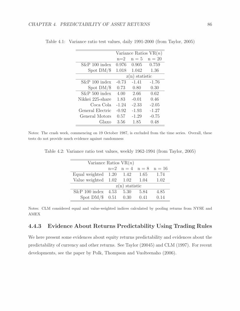
CHAPTER 4. PREDICTABILITY OF ASSET RETURNS 86
Table 4.1: Variance ratio test values, daily 1991-2000 (from Taylor, 2005)
Variance Ratios VR(n)n=2 n = 5 n = 20
S&P 100 index 0.976 0.905 0.759Spot DM/$ 1.018 1.042 1.36
z(n) statisticS&P 100 index -0.73 -1.41 -1.76
Spot DM/$ 0.73 0.80 0.30S&P 500 index 4.00 2.66 0.62
Nikkei 225-share 1.83 -0.01 0.46Coca Cola -1.24 -2.33 -2.05
General Electric -0.92 -1.93 -1.27General Motors 0.57 -1.29 -0.75
Glaxo 3.56 1.85 0.48
Notes: The crash week, commencing on 19 October 1987, is excluded from the time series. Overall, these
tests do not provide much evidence against randomness
Table 4.2: Variance ratio test values, weekly 1962-1994 (from Taylor, 2005)
Variance Ratios VR(n)n=2 n = 4 n = 8 n = 16
Equal weighted 1.20 1.42 1.65 1.74Value weighted 1.02 1.02 1.04 1.02
z(n) statisticS&P 100 index 4.53 5.30 5.84 4.85
Spot DM/$ 0.51 0.30 0.41 0.14
Notes: CLM considered equal and value-weighted indices calculated by pooling returns from NYSE and
AMEX
4.4.3 Evidence About Returns Predictability Using Trading Rules
We here present some evidences about equity returns predictability and evidences about the
predictability of currency and other returns. See Taylor (20045) and CLM (1997). For recent
developments, see the paper by Polk, Thompson and Vuolteenaho (2006).
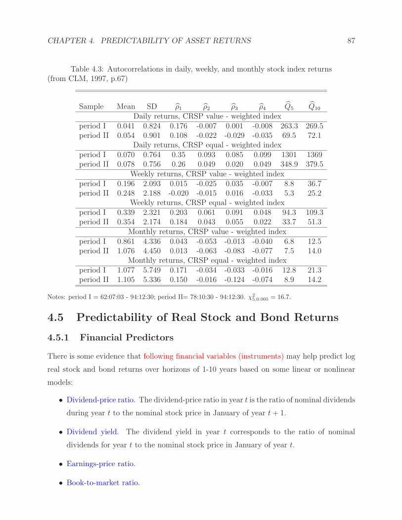
CHAPTER 4. PREDICTABILITY OF ASSET RETURNS 87
Table 4.3: Autocorrelations in daily, weekly, and monthly stock index returns(from CLM, 1997, p.67)
Sample Mean SD ρ1 ρ2 ρ3 ρ4 Q5 Q10
Daily returns, CRSP value - weighted indexperiod I 0.041 0.824 0.176 -0.007 0.001 -0.008 263.3 269.5period II 0.054 0.901 0.108 -0.022 -0.029 -0.035 69.5 72.1
Daily returns, CRSP equal - weighted indexperiod I 0.070 0.764 0.35 0.093 0.085 0.099 1301 1369period II 0.078 0.756 0.26 0.049 0.020 0.049 348.9 379.5
Weekly returns, CRSP value - weighted indexperiod I 0.196 2.093 0.015 -0.025 0.035 -0.007 8.8 36.7period II 0.248 2.188 -0.020 -0.015 0.016 -0.033 5.3 25.2
Weekly returns, CRSP equal - weighted indexperiod I 0.339 2.321 0.203 0.061 0.091 0.048 94.3 109.3period II 0.354 2.174 0.184 0.043 0.055 0.022 33.7 51.3
Monthly returns, CRSP value - weighted indexperiod I 0.861 4.336 0.043 -0.053 -0.013 -0.040 6.8 12.5period II 1.076 4.450 0.013 -0.063 -0.083 -0.077 7.5 14.0
Monthly returns, CRSP equal - weighted indexperiod I 1.077 5.749 0.171 -0.034 -0.033 -0.016 12.8 21.3period II 1.105 5.336 0.150 -0.016 -0.124 -0.074 8.9 14.2
Notes: period I = 62:07:03 - 94:12:30; period II= 78:10:30 - 94:12:30. χ2
5,0.005= 16.7.
4.5 Predictability of Real Stock and Bond Returns
4.5.1 Financial Predictors
There is some evidence that following financial variables (instruments) may help predict log
real stock and bond returns over horizons of 1-10 years based on some linear or nonlinear
models:
• Dividend-price ratio. The dividend-price ratio in year t is the ratio of nominal dividends
during year t to the nominal stock price in January of year t+ 1.
• Dividend yield. The dividend yield in year t corresponds to the ratio of nominal
dividends for year t to the nominal stock price in January of year t.
• Earnings-price ratio.
• Book-to-market ratio.

CHAPTER 4. PREDICTABILITY OF ASSET RETURNS 88
• Federal q. This is the ratio of the total market value of equities outstanding to corporate
net worth.
• Payout ratio. Ratio of the dividends to the earnings
• Term spread. This is difference between annualized long-term and short-term govern-
ment yield.
• Default spread. This is difference between Moody’s seasoned Baa corporate bond yield
and the Moody’s seasoned Aaa corporate bond yield
• Short-term rate. This is the 3-month Treasure bill rate (secondary market)
• · · ·
4.5.2 Models and Modeling Methods
Introduction
The predictability of stock returns has been studied for decades as a cornerstone research
topic in economics and finance. See, for example, Fama and French (1988), Keim and
Stambaugh (1986), Campbell and Shiller (1988), Cutler, Poterba, and Summers (1991),
Balvers, Cosimano, and McDonald (1990), Schwert (1990), Fama(1990), and Kothari and
Shanken (1997). In many financial applications such as the mutual fund performance, the
conditional capital asset pricing, and the optimal asset allocations, people routinely examine
the predictability problem. See, for example, Christopherson et al. (1998), Ferson and Schadt
(1996), Ferson and Harvey (1991), Ghysels (1998), Ait-Sahalia and Brandt (2001), Barberis
(2000), Brandt (1999), Campbell and Viceira (1998), and Kandel and Stambaugh (1996).
Tremendous empirical studies document the predictability of stock returns using various
lagged financial variables, such as the dividend yield, the term spread and default premia,
the dividend-price ratio, the earning-price ratio, the book-to-market ratio, and the interest
rates. Important questions are often asked about whether the returns are predictable and
whether the predictability is stable over time. Since many of the predictive financial variables
are highly persistent and even nonstationary, it is really challenging statistically to answer
these questions.
The predictability issues are generally assessed in the context of parametric predictive
regression models in which rates of returns are regressed against the lagged values of stochas-

CHAPTER 4. PREDICTABILITY OF ASSET RETURNS 89
tic explanatory variables (or state variables). Now let us review the efforts in literature on
this topic. Mankiw and Shapiro (1986) and Stambaugh (1986) were the first to discern
the econometric (statistical) difficulties inherent in the estimation of predictive regressions
through the structure predictive linear model:
yt = µ1 + βxt−1 + εt, xt = ρxt−1 + ut, 1 ≤ t ≤ n, (4.13)
where innovations (εt, ut) are independently and identically distributed bivariate normal
N(0,Σ) with Σ =
(σ2ε σεu
σεu σ2u
), yt is the predictable variable, say excess stock returns, in
period t, and xt−1 is a financial variable such as the log dividend-price ratio at t−1, which is
commonly modeled by an AR(1) model as in (4.13). Note that the correlation between the
innovations is δ = σεu/σεσu, which is unfortunately non-zero for many empirical applications;
see Table 4 in Campbell and Yogo (2006) and Table 1 in Paye and Timmermann (2006).
This creates the endogeneity (xt−1 and εt are correlated) which makes modeling difficult.
The parameter ρ is the unknown degree of persistence of the variable xt. That is, xt is
stationary (|ρ| < 1); see Amihud and Hurvich (2004) and Paye and Timmermann (2006),
or it is local-to unity or nearly integrated (ρ = 1 + c/n with c < 0), or it is unit root or
integrated (denoted by I(1)) (ρ = 1). See, for example, Elliott and Stock (1994), Cavanagh,
Elliott, and Stock (1995), Torous, Valkanov, and Yan (2004), Campbell and Yogo (2006),
Polk, Thompson, and Vuolteenho (2006), and Rossi (2007), among others. This means that
predictive variable xt is highly persistent, not really exogenous, and even nonstationary,
which causes a lot of troubles for statistical modeling.
As shown in Nelson and Kim (1993), the ordinary least squares (OLS) estimates of the
slope coefficient β and its standard errors are substantially biased in finite samples if xt is
highly persistent, not really exogenous, and even nonstationary. Conventional tests based
on standard t-statistics from OLS estimates tend to over-reject the null of non-predictability
in the Monte-Carlo simulations, although some improvements were developed recently.
In an effort to dealing with the aforementioned difficulties associated with the endogeneity
and to obtaining efficient inference about the coefficient β, researchers have made their
contributions, summarized as follows:
(1) The bias correction of the OLS estimate, using information conveyed by the autoregres-
sive process of the predictive variable. See, for example, the first order bias-corrected
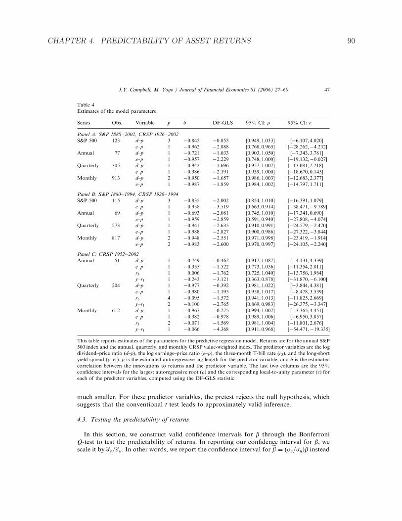
CHAPTER 4. PREDICTABILITY OF ASSET RETURNS 90
much smaller. For these predictor variables, the pretest rejects the null hypothesis, which
suggests that the conventional t-test leads to approximately valid inference.
4.3. Testing the predictability of returns
In this section, we construct valid confidence intervals for b through the Bonferroni
Q-test to test the predictability of returns. In reporting our confidence interval for b, we
scale it by bse=bsu. In other words, we report the confidence interval for eb ¼ ðse=suÞb instead
ARTICLE IN PRESS
Table 4
Estimates of the model parameters
Series Obs. Variable p d DF-GLS 95% CI: r 95% CI: c
Panel A: S&P 1880– 2002, CRSP 1926– 2002
S&P 500 123 d–p 3 0.845 0.855 ½0:949; 1:033 ½6:107; 4:020e–p 1 0.962 2.888 ½0:768; 0:965 ½28:262;4:232
Annual 77 d–p 1 0.721 1.033 ½0:903; 1:050 ½7:343; 3:781
e–p 1 0.957 2.229 ½0:748; 1:000 ½19:132;0:027Quarterly 305 d–p 1 0.942 1.696 ½0:957; 1:007 ½13:081; 2:218
e–p 1 0.986 2.191 ½0:939; 1:000 ½18:670; 0:145
Monthly 913 d–p 2 0.950 1.657 ½0:986; 1:003 ½12:683; 2:377
e–p 1 0.987 1.859 ½0:984; 1:002 ½14:797; 1:711
Panel B: S&P 1880– 1994, CRSP 1926– 1994
S&P 500 115 d–p 3 0.835 2.002 ½0:854; 1:010 ½16:391; 1:079e–p 1 0.958 3.519 ½0:663; 0:914 ½38:471;9:789
Annual 69 d–p 1 0.693 2.081 ½0:745; 1:010 ½17:341; 0:690
e–p 1 0.959 2.859 ½0:591; 0:940 ½27:808;4:074Quarterly 273 d–p 1 0.941 2.635 ½0:910; 0:991 ½24:579;2:470
e–p 1 0.988 2.827 ½0:900; 0:986 ½27:322;3:844
Monthly 817 d–p 2 0.948 2.551 ½0:971; 0:998 ½23:419;1:914
e–p 2 0.983 2.600 ½0:970; 0:997 ½24:105;2:240
Panel C: CRSP 1952– 2002
Annual 51 d–p 1 0.749 0.462 ½0:917; 1:087 ½4:131; 4:339e–p 1 0.955 1.522 ½0:773; 1:056 ½11:354; 2:811
r3 1 0.006 1.762 ½0:725; 1:040 ½13:756; 1:984
y–r1 1 0.243 3.121 ½0:363; 0:878 ½31:870;6:100Quarterly 204 d–p 1 0.977 0.392 ½0:981; 1:022 ½3:844; 4:381
e–p 1 0.980 1.195 ½0:958; 1:017 ½8:478; 3:539
r3 4 0.095 1.572 ½0:941; 1:013 ½11:825; 2:669
y–r1 2 0.100 2.765 ½0:869; 0:983 ½26:375;3:347Monthly 612 d–p 1 0.967 0.275 ½0:994; 1:007 ½3:365; 4:451
e–p 1 0.982 0.978 ½0:989; 1:006 ½6:950; 3:857
r3 2 0.071 1.569 ½0:981; 1:004 ½11:801; 2:676
y–r1 1 0.066 4.368 ½0:911; 0:968 ½54:471;19:335
This table reports estimates of the parameters for the predictive regression model. Returns are for the annual S&P
500 index and the annual, quarterly, and monthly CRSP value-weighted index. The predictor variables are the log
dividend–price ratio (d–p), the log earnings–price ratio (e–p), the three-month T-bill rate (r3), and the long-short
yield spread (y–r1). p is the estimated autoregressive lag length for the predictor variable, and d is the estimated
correlation between the innovations to returns and the predictor variable. The last two columns are the 95%
confidence intervals for the largest autoregressive root (r) and the corresponding local-to-unity parameter (c) for
each of the predictor variables, computed using the DF-GLS statistic.
J.Y. Campbell, M. Yogo / Journal of Financial Economics 81 (2006) 27–60 47
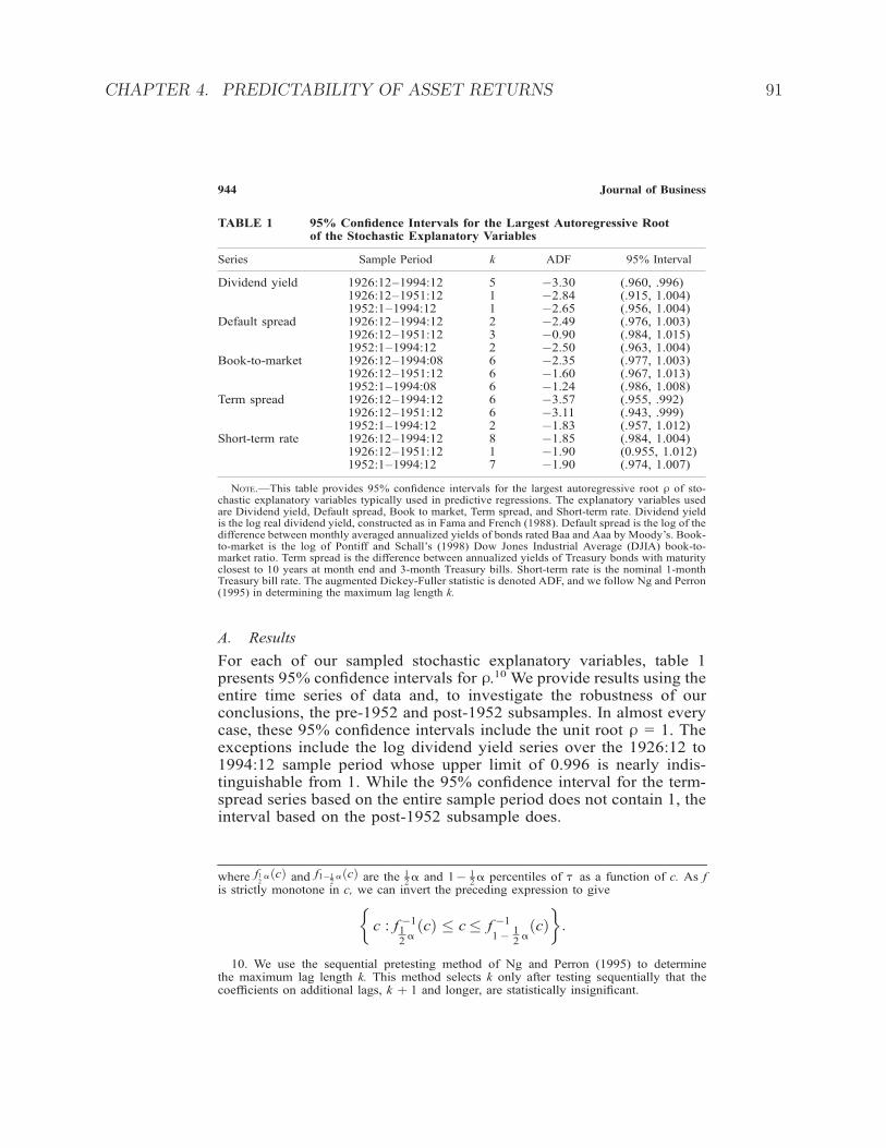
CHAPTER 4. PREDICTABILITY OF ASSET RETURNS 91
A. Results
For each of our sampled stochastic explanatory variables, table 1presents 95% confidence intervals for U.10 We provide results using theentire time series of data and, to investigate the robustness of ourconclusions, the pre-1952 and post-1952 subsamples. In almost everycase, these 95% confidence intervals include the unit root U = 1. Theexceptions include the log dividend yield series over the 1926:12 to1994:12 sample period whose upper limit of 0.996 is nearly indis-tinguishable from 1. While the 95% confidence interval for the term-spread series based on the entire sample period does not contain 1, theinterval based on the post-1952 subsample does.
TABLE 1 95% Confidence Intervals for the Largest Autoregressive Rootof the Stochastic Explanatory Variables
Series Sample Period k ADF 95% Interval
Dividend yield 1926:12–1994:12 5 3.30 (.960, .996)1926:12–1951:12 1 2.84 (.915, 1.004)1952:1–1994:12 1 2.65 (.956, 1.004)
Default spread 1926:12–1994:12 2 2.49 (.976, 1.003)1926:12–1951:12 3 0.90 (.984, 1.015)1952:1–1994:12 2 2.50 (.963, 1.004)
Book-to-market 1926:12–1994:08 6 2.35 (.977, 1.003)1926:12–1951:12 6 1.60 (.967, 1.013)1952:1–1994:08 6 1.24 (.986, 1.008)
Term spread 1926:12–1994:12 6 3.57 (.955, .992)1926:12–1951:12 6 3.11 (.943, .999)1952:1–1994:12 2 1.83 (.957, 1.012)
Short-term rate 1926:12–1994:12 8 1.85 (.984, 1.004)1926:12–1951:12 1 1.90 (0.955, 1.012)1952:1–1994:12 7 1.90 (.974, 1.007)
Note.—This table provides 95% confidence intervals for the largest autoregressive root U of sto-chastic explanatory variables typically used in predictive regressions. The explanatory variables usedare Dividend yield, Default spread, Book to market, Term spread, and Short-term rate. Dividend yieldis the log real dividend yield, constructed as in Fama and French (1988). Default spread is the log of thedifference between monthly averaged annualized yields of bonds rated Baa and Aaa by Moody’s. Book-to-market is the log of Pontiff and Schall’s (1998) Dow Jones Industrial Average (DJIA) book-to-market ratio. Term spread is the difference between annualized yields of Treasury bonds with maturityclosest to 10 years at month end and 3-month Treasury bills. Short-term rate is the nominal 1-monthTreasury bill rate. The augmented Dickey-Fuller statistic is denoted ADF, and we follow Ng and Perron(1995) in determining the maximum lag length k.
where f12aðcÞ and f11
2aðcÞ are the 1
2a and 1 1
2a percentiles of H as a function of c. As f
is strictly monotone in c, we can invert the preceding expression to give
c : f 112a
ðcÞ c f 1
112a
ðcÞ
:
10. We use the sequential pretesting method of Ng and Perron (1995) to determinethe maximum lag length k. This method selects k only after testing sequentially that thecoefficients on additional lags, k þ 1 and longer, are statistically insignificant.
944 Journal of Business

CHAPTER 4. PREDICTABILITY OF ASSET RETURNS 92
OLS estimator in Kothari and Shanken (1997) and Stambaugh (1999), the second or-
der bias-correction method in Amihud and Hurvich (2004), and the conservative bias-
correction method in Lewellen (2004) which assumes the true autoregressive coefficient
of AR(1) to be close to one.
(2) Econometric inferences about the linear regression coefficient β. The inference for the
slope coefficient is unreliable, due to the discontinuity in the asymptotic distribution
of the estimator of the I(1) or nearly I(1) autoregressive coefficient ρ of the predictive
variable which is often persistent and nonstationary. This is another difficulty for
modeling predictive regression models. In finite samples, this problem thwarts the
drawing of correct inference of the slope coefficient β even when the coefficient in an
AR(1) process is close to, but not necessarily equal to, one. In the literature, people
seek more accurate sampling distributions of test statistics. Some apply the exact finite-
sample theory under the assumption of normality, (see Kothari and Shanken (1997),
Stambaugh(1999), and Lewellen (2004), among others) and others employ nearly I(1)
asymptotics to approximate the finite sample distributions. It is noteworthy that these
hypothesis testing procedures are all based on the biased OLS coefficient estimates.
Note that OLS estimates of the coefficient in predictive linear regression are also widely
used in finance literature on out-of-sample forecasting; see Goyal and Welch (2003a,b).
(3) The instability of return forecasting models. In fact, in forecasting models for the
dividend and earnings yield, the short interest rate, and the term spread and default
premium, there have been found many evidences on instability of prediction in the
second half of the 1990s, which lead to the conclusion that the coefficients should
change over time; see Lettau and Ludvigsson (2001), Goyal and Welch (2003a), Paye
and Timmermann (2006), and Ang and Bekaert (2007).
However, existing approaches may not be appropriate in many real applications due to
restrictive assumptions on the functional forms in regression. In fact, the above studies
are mostly based on linear predictive models and produce biased and inefficient estimates,
especially when the predictive variable follows an AR(1) model with the innovation highly
correlated with the error series of the return (endogenous). In addition, most studies assume
that the coefficients of the state variables are fixed over time, which may not hold in practice.
CHAPTER 4. PREDICTABILITY OF ASSET RETURNS 93
Recent empirical studies have cast doubt upon the constant-coefficient assumption; see Goyal
and Welch (2003a) and Paye and Timmermann (2006).
To tackle the above problems, I would like to point out a host of new semiparametric
and nonparametric modeling techniques to reduce possible modeling biases in the paramet-
ric predictive regression models and to capture time-varying dynamics of the returns. New
models and cutting-edge technologies will be introduced to check the predictability of re-
turns and to test the stability of predictability which have been puzzling us since 1980s.
The proposed models belong to the nonlinear additive time series models and time-varying
coefficient models but with possibly highly persistent, not really exogenous, and even nonsta-
tionary financial predictors. As expected, they will avoid misspecification and produce more
accurate and efficient estimates of the true functions. Fundamental theoretical results for
the proposed methodology will be established, which will enrich the theory of statistics and
econometrics, enlarge the scope of application of nonparametric/semiparametric modeling,
and improve understanding of predictability of returns.
Finally, it is necessary to point out the differences between classical (standard) nonpara-
metric regression models [see Fan and Yao (2003)] and nonlinear predictive regression models
proposed in this proposal. The biggest difference is that the latter involves the endogene-
ity (predetermined) and persistent and nonstationary (nearly integrated or I(1)) predictive
variables, which make the asymptotic analysis of the associated estimators much more chal-
lenging. As we aware of, there are no any theoretical results available in the literature for
nonparametric/semiparametric predictive regression models.
Existing Methods for Predictive Regression Models
For simplicity, we follows the notation in Campbell and Yogo (2006) and consider a single-
variable predictive regression model formulated in (4.13), which postulates the structure
relationship between xt−1 and yt.
The main effort in the literature is to estimate β efficiently and to test if the returns are
predictable using the state variable, which amounts to testing the null hypothesis H0 : β = 0,
treating µ1 and ρ as nuisance parameters. Due to the non-zero correlation between εt and
ut, this model violates the classical OLS assumption of independence between variable xt−1
and error εt at all leads and lags. Therefore, the OLS estimates, β and ρ, are biased, and
CHAPTER 4. PREDICTABILITY OF ASSET RETURNS 94
the biases of the two estimators are closely related, since E[β − β
]= γ E [ρ− ρ], where
γ = δ σε/σu. Furthermore, the persistent financial variable xt renders difficulties in making
inference about predictability. Even if the predictor variable xt is indeed I(0), the first-order
asymptotics can be a poor approximation when ρ is close to one. This is because of the
discontinuity in the asymptotic distribution at ρ = 1 where the variance of xt diverges to
infinity. Inference about β based on the first order asymptotics, such as conventional t-tests,
is therefore invalid due to large size distortions; see the aforementioned papers for details.
In what follows, I briefly delineate the existing mainstream approaches to dealing with
the bias-correction and inference problems. Clearly, the finite sample bias in β comes from
the bias of the autoregressive estimation of ρ and is magnified by γ. A common solution
is to obtain a more precise finite sample approximation to the bias of ρ by utilizing the
bias-corrected estimate of ρ. This includes the following three methods:
(i) The first order bias-correction estimator in Stambaugh (1999), βc = β + γ (1 + 3ρ)/n,
where γ = σεu/σ2u, and ε and u are all obtained from OLS estimation. This estimator is
obtained based on Kendall (1954)’s analytical result, E(ρ−ρ) = −(1+3 ρ)/n+O(n−2).
(ii) The two-stage least squares method in Amihud and Hurvich (2004). Assuming ρ < 1
and a linear relationship between εt and ut (indeed, the projection of εt onto ut) as
εt = θ ut + vt, (4.14)
the predictive regression model (4.13) can be rewritten as
yt = µ1 + β xt−1 + θ ut + vt, (4.15)
where vt is white noise independent of both xt and ut at all leads and lags. The
regression thus meets the classical assumption of OLS without endogeneity if ut were
known. This motivated Amihud and Hurvich (2004) to obtain the OLS estimate of ρ
first and then to regress yt on xt−1 and the fitted residuals ut to obtain a bias-corrected
estimate β∗, which is indeed a second order bias-correction method.
(iii) The conservative bias-adjusted estimator in Lewellen (2004), β∗∗ = β + γ (0.9999− ρ)
when ρ is very close to one. It can be showed easily that β∗∗ must be the least biased
estimator of β when the true ρ is indeed very close to one.

CHAPTER 4. PREDICTABILITY OF ASSET RETURNS 95
While these methods evidence the predictability of returns, they have at least the following
drawbacks. First, they work under the linear relationship between the return and the state
variables which may not hold. Second, they do not consider instability issues (coefficients in
the predictive models might change over time). For example, they do not determine if the
coefficients might change over time where the return models may have changed, nor do they
consider the possibility of structural breaks or the time of their occurrence. These important
issues should be addressed. See, for example, Bossaerts and Hillion (1999), Sullivan, Tim-
mermann and White (1999), Marquering and Verbeek (2004), and Cooper, Gutierrez and
Marcum (2005). Furthermore, if financial prediction models are evolving (unstable) over
time, the economic significance of return predictability can only be assessed provided it is
determined how widespread such instability is both internationally and over time and the
extent to which it affects the predictability of stock returns. To investigate these problems,
using a sample of excess returns for international equity indices, Paye and Timmermann
(2006) analyzed both how widespread the evidence of structural breaks is and to what ex-
tent the breaks affect the predictability of stock returns. Also, Inoue and Kilian (2004)
showed that tests based on in-sample predictability typically are much more powerful than
out-of-sample tests which generally use much smaller sample sizes. Indeed, it is possible that
the absence of strong out-of-sample predictability in stock returns is entirely due to the use
of relatively short evaluation samples. Using the full sample for analysis, Paye and Timmer-
mann (2006) argued that there is a sufficient power to address whether this explanation is
valid or whether predictability genuinely has declined over time.
4.6 A Recent Perspective on Predictability of Asset
Return
To summarize the above and to see what the future should be in this direction, I strongly
recommend you should read the following paper by the Nobel Laureate in Economics in 2003
Professor Clive W.J. Granger, which appeared in Journal of Econometrics (2005). As you
might know, Professor Clive Granger received the Nobel Prize in economics in 2003 due to
his contributions in Time Series Econometrics.

CHAPTER 4. PREDICTABILITY OF ASSET RETURNS 96
4.6.1 Introduction
Granger and Morgenstern (1970) published a book about the “Forecastability of Stock Mar-
ket Prices”, generally using lower frequency (say, daily or weekly or monthly) data to test
the random walk theory using autocorrelations and spectra. However, they did also consider
high-frequency transaction (say, tick-by-tick) data plus dividends and earnings in macro-
economic relationships.
Unsurprisingly, we found that returns are difficult to forecast, except in the very short-run
and the very long-run. In the third of a century since the book appeared empirical finance
has changed dramatically from just a few active workers to hundreds, maybe thousands.
The number of finance journals changed from one dozens and the techniques have become
considerably more advanced. The availability of much more data and greatly increased
computer power has produced more impressive research publications. It can be argued that
many of these publications have relatively little practical usefulness. In fact the purpose
of much of the work is unclear. Papers still keep appearing that reaffirm the random walk
theory. Of course, if a researcher had discovered a method of successfully forecasting returns,
she would not have published it, but would have accumulated considerable wealth. It may
well have happened, and we just do not know.
Occasionally, papers are published suggesting how returns can be forecast using a simple
statistical model, and presumably these techniques are the basis of the decisions of some
financial analysts. More likely the results are fragile, once you try to use them, they go away.
There now exists several excellent textbooks on financial econometrics and they generally
do a good job of surveying the safe features of the most popular procedures. I plan to
take a rather more realistic and forward looking viewpoint on the available and forthcoming
techniques. I will use four sections, about conditional means, conditional variances, then
conditional distributions, and finally, the future.
4.6.2 Conditional Means
The original objective of much of the empirical financial research concentrated on mean
returns, conditional on previous returns, and possibly on other economic variables. Only
quite recently has the pair of return and volume be modelled jointly, as would be suggested by
a micro-economics text. Most of the techniques considered are those developed in statistical
CHAPTER 4. PREDICTABILITY OF ASSET RETURNS 97
and macro time series analysis, that is autoregressive models, VARs, unit root models,
cointegration, seasonality, and the usual bundle of nonlinear models, including chaos, neural
networks, and various other nonlinear autoregressive models. Some of these models seem to
be relevant and helpful, most do not.
Quite a lot of attention has been given to a property known as “long-memory,” in which
autocorrelations decline very slowly compared to any simple autoregressive model. It is
observed that the autocorrelations of measures of volatility, such as |rt|d, where rt is a
return series and d is positive, have the long-memory property. This observation, which
is wide-spread and occurs for many assets and markets, has produced a misinterpretation.
Theoretical results show that the fractional integrated (I(d)) model has the long-memory
property, and so it was concluded that any process with this property must be an I(d)
process. However, the conclusion is incorrect as pointed out in Granger (2000) and elsewhere,
as other processes can produce long-memory, particularly processes with breaks. If Xt is a
positive process, and therefore has positive mean, if it is I(d); it must have a mean that is
proportional to td ; and so will have a distinct trend in mean. As volatility has no such trend
it cannot be I(d); especially as the “estimated” value of d is often found to be near 1/2. It
follows that the I(d) model is not appropriate for volatility but a break model remains a
plausible candidate to explain the observed long-memory property.
There have been several papers pointing out that a stationary process with occasional
level shifts will have the long memory properties, for example Granger and Hyung (2004)
(based on Hyung’s 1999 Ph.D. thesis) and Diebold and Inoue (2001). The breaks need to
be not too frequent but stochastic in magnitude. A break process considered by Hyung and
Franses (2002) takes the form
yt = mt + ǫt, mt = mt−1 + qt ηt (4.16)
with ǫt, ηt being zero mean, white noise and where qt follows an i.i.d. binomial t distribution,
so that qt = 1 with probability p, qt = 0 with a probability of 1− p. The expected number
of breaks is affected by p and the magnitude of σ2η. The break processes for stock prices
produces returns with a longer-tailed distribution but volatilities such as absolute returns
that do not suffer from the trending problem. These volatilities are found to fit as well, if
not better in other respects, than an I(d) model, by Granger and Hyung (2004).
CHAPTER 4. PREDICTABILITY OF ASSET RETURNS 98
4.6.3 Conditional Variances
If one wants to describe a distribution, just knowing the mean is totally inadequate, knowing
the mean and variance is clearly better. For those of us interested in empirical studies, our
immediate problem is that variance is not easily observed. One can form a sum of squared
deviations of returns around a mean but they take time to accumulate. The ARCH class
of models partly circumvents this problem and provides quite up-to-date values for the
variance. The purpose of measuring variance is somewhat less clear, particularly as returns
have been shown, consistently to have non-Gaussian distributions. The part of economics
that discusses uncertainty, risk, and insurance have for many years emphasized that measures
of volatility based on E(|rt|d) for positive d are quite inappropriate measures of risk. The
topic is mentioned in Granger (2002). The problem is easy to illustrate. Suppose a small
portfolio experiences a large negative shock to an asset, this will be treated as an increase
in risk, as it increases the chance of selling the asset at a lower price that its purchase price.
However, if an asset receives a large positive price shock, this is considered an increase in
uncertainty, but not in risk. However, both shocks will produce an increase in variance,
which treats movements in either tail of the distribution equally, although only those on one
side are undesirable. Measurements of risk based on quantiles, such as “Value-at-Risk,” or
VaR, avoid such problems as does the semi-variance suggested by Markowitz in his original
book on portfolio theory.
4.6.4 Distributions
The next obvious step is towards using predictive, or conditional, distributions. Major
problems remain, particularly with parametric forms and in the multivariate case. For
the center of the distribution a mixture of Gaussians appears to work well but these do
not represent tail probabilities in a satisfactory fashion. By thinking about a multivariate
distribution written in terms of marginals and a rectangular copula, it seems that all tail
properties will come from the marginals. A very practical time-series approach to conditional
distributions is to model quantiles, which can take autoregressive forms, have breaks, unit
roots, and other driving variables. Modeling and estimation is not very difficult and in
practice the problem of estimated quantiles crossing appears not to be difficult (see Granger
and Sin, 2000). The observed long-memory properties of volatility should be observed in the
quantiles due to breaks.
CHAPTER 4. PREDICTABILITY OF ASSET RETURNS 99
4.6.5 The future
The immediate future in any active academic field always involves topics that have already
started. I believe that conditional distributions will continue to be a major subject as finance
learns how to generate of its fundamental theories into distributional forms, arbitrage, port-
folio theory, efficient market theory and consequences, Black-Scholes formula, and so forth.
This will be an exciting period and very general results will appear and new testing methods
devised. It is also likely that there will be structural breaks in the present framework, but
such breaks are difficult to forecast, which is the basic element of their nature. However,
there are two I think may be seen; the first is a new approach to volatility and the second
is a reformulation of basic functional theory. Most of the old literature on prices, returns,
and volatility had, basically, a linear foundation. From studying the models suggested by
these approaches a number of “stylized facts” have been accumulated, these being empirical
“facts” that have been observed to occur for many (possibly all) assets in most (possibly all)
markets, most time periods and most data frequencies. A list of these stylized facts would
include:
(i) Returns are nearly white noise; that is, they have no serial or auto correlation.
(ii) The autocorrelations of r2t and |rt|d decline slowly with increasing lag long memory
effect.
(iii) Similarly, the autocorrelations of |rt|d decline slowly, with the slowest decline for
d = 1 (Taylor effect).
(iv) Autocorrelations of sign rt are all small, insignificant.
(v) If one fits a GARCH(1, 1) model to the series, then α + β ≈ 1, with the usual
notation.
In a remarkable paper, Yoon (2003) shows, largely by simulation, that the simple stochas-
tic unit root model
Pt = (1 + at)Pt−1 + ǫt,
where Pt is log stock price and at, ǫt are independent white noise series produces returns series
that have all of the stylized facts observed with actual data. It does not imply that actual
log stock prices are generated by this model, but it does suggest that it can capture many

CHAPTER 4. PREDICTABILITY OF ASSET RETURNS 100
realistic properties in a very simple model, and so deserves further study. Yoon’s model is
an example of a “stochastic unit root process” as discussed by Granger and Swanson (1997),
Leybourne, McCabe and Mills (1996), and Leybourne, McCabe and Tremayne (1996). Yoon
considers a particularly simple case where at is a zero mean i.i.d. sequence and ǫt is a zero
mean white noise.
Let me finally turn to an area in which I do not claim to have much special knowledge,
continuous time finance theory. I have looked over a number of books in the area and note
that much of the work starts with an assumption that a price or a return can be written in
terms of a standard diffusion, which is based on a Gaussian distribution.
This immediately brings up warning signals because much of early econometrics used a
similar Gaussian assumption, just for mathematical convenience, and without proper test-
ing. Occasionally, it was asked if a marginal distribution could pass a test with a null of
Gaussianity, but I never saw a joint test of normality, which was really needed for much of
the theory to be operative. For the continuous time theory there is effectively no evaluation
of the theory using empirical tests because there is no continuous time data. When the
theory is brought over to discrete time, it is unclear if it continues to hold. There could be
a bifurcation in going from continuous to discrete time. Ito’s lemma, which uses a Gaussian
assumption, I believe, need no longer work in the discrete time zone. In fact the majority of
the empirical work that I have seen appears to find that in the highest frequency data the
best models do not agree with continuous time theory.
Some recent work by Aıt-Sahalia (2002) suggests that the discrete data results are more
consistent with jump-diffusions, that is diffusions with breaks, rather than standard diffu-
sions. If further evidence for that result is accumulated, it is likely that the majority of
current financial theory will have to be rewritten, with “jump-diffusion” replacing “diffu-
sion,” and with some consequent changes in theorems and results. As a great deal of human
capital will be devalued by such a development, it will certainly be opposed by many editors
and referees, as happens with all radical new ideas.

CHAPTER 4. PREDICTABILITY OF ASSET RETURNS 101
4.7 Comments on Predictability Based on Nonlinear
Models
The aforementioned predictability of asset returns is mainly on linear models but not much
on nonlinear models. As advocated by Granger (2005), nonlinear conditional mean functions
might be a good way to be explored, as in Hyung and Franses (2002) or model (4.16), which
can be regarded as the threshold type model, a special case of nonlinear models. Of course,
other types of nonlinear forms are warranted for a further study or they can be regarded as
a future research topic. To explore a possible research topic, you may have an interest in
exploring the data set in the data file “SP-A.txt” [The first column is the return for S&P
500 CRSP weighted value and the second column is the log dividend-price ratio and the
third column is the log earnings-price ratio], which can be downloaded from the course web
site. As mentioned in Chapter 2, Hong and Lee (2003) conducted studies on exchange rates
and they found that some of them are predictable based on nonlinear time series models.
There are many ongoing research activities in this direction. See Chapter 4 in Tsay (2005),
Chapter 12 of Campbell, Lo and MacKinlay (1997), and the book by Fan and Yao (2003).
If we have time, we will come back to this topic later.
4.8 Problems
4.8.1 Exercises for Homework
1. Please download weekly (daily) price data for any stock, for example, Microsoft (MSFT)
stock (Pt) for 03/13/1986 - 02/15/2008.
2. Estimate the CER model for Microsoft using the OLS estimation and construct a series
of residuals: et = rt − µ.
(a) Compute the autocorrelation function (ACF) of the residuals, ρk10k=1. Graph the
auto- correlation coefficients and confidence intervals around them. What does it
suggest about autocorrelation in returns and predictability of returns?
(b) Test the following null hypothesis: (i) H0 : ρ1 = 0, (ii) H0 : ρ2 = 0, and (iii)
H0 : ρ7 = 0.
(c) Use the modified Ljung-Box Q-test defined in equation (4.7) for testing autocorre-
lation. In testing, set the number of autocorrelations used m = 10. This modified

CHAPTER 4. PREDICTABILITY OF ASSET RETURNS 102
Q-test will give you different results from the results on Q-test in the previous
problem because the test statistic is different.
(d) Use the variance ratio statistic VR(n) in equation (4.8) to test for predictability in
stock returns. The variance ratio statistic can be computed using R. The program
also computes the standardized variance ratio statistic which follows a standard
normal distribution. Present your results and comment on predictability of MSFT
stock returns.
(e) Consider the following model for MSFT prices: pt = pt−1 + et. Use CJ test
statistic to test the predictability of MSFT prices. Are your results as expected?
You may mention your results of significance test of µ in Problem 5 in Chapter 3.
3. Use autocorrelation tests and variance ratio tests to check predictability for IBM,
Coca-Cola, Glaxo stock returns for both weekly and daily for the period 03/13/1986 -
2/15/2008. Comment your results.
4. Use autocorrelation tests and variance ratio tests to check predictability of S&P500
index and DJIA index for weekly and daily for the period 03/13/1986 - 2/15/2008.
Comment your results.
5. Assume that you have an equal weighted portfolio that consists of four stocks: IBM,
Microsoft, Coca-Coal, and Glaxo for both weekly and daily. For the period 03/13/1986
- 2/15/2008, construct portfolio returns of this portfolio and conduct autocorrelation
and variance ratio tests of predictability. Comment your results.
4.8.2 R Codes
# 2-13-2008
# R code for computing the p-value for Cowles-Jones test
data=read.csv(file="c:/zcai/res-teach/econ6219/Bank-of-America.csv",header=T)
x=data[,5] # get the closing prices
x=rev(x) # reverse
n=length(x) # sample size
rt=diff(log(x)) # log return
rt_0=rt-mean(rt) # centerized
n1=length(rt_0)

CHAPTER 4. PREDICTABILITY OF ASSET RETURNS 103
I_t=(rt_0>0) # indicator for return is positive
n2=n1-1
I_t1=I_t[2:n1]
Y_t=I_t[1:n2]*I_t1+(1-I_t[1:n2])*(1-I_t1) # compute Y_t
n_s=sum(Y_t) # number of Y_t=1
n_r=n2-n_s
cj=n_s/n_r # CJ statistic
z=sqrt(n2)*abs(cj-1) # Z-score
p_value=2*(1-pnorm(z)) # p-value
print(c("The p-value for Cowles-Jones test is", p_value))
# Variance Ratio Test
library(vrtest) # load package
kvec1=c(2,5,10,20)
LM_test=Lo.Mac(rt,kvec1)
print(c("Results for Lo-MacKinlay test:", LM_test))
4.8.3 Project #1
1. Read the article “Efficient Capital Markets: II” by Fama (1991).
(a) Briefly describe the main results of the literature on the predictability of short-run
returns.
(b) Briefly describe the main results of the literature on the predictability of long-run
returns.
2. Read Chapter 7 of Taylor (2005). Briefly explain the main findings about the pre-
dictability of equities, currencies, and futures based on trading rules analysis.
3. After you read the survey paper by Granger (2005), please think about some possible
and interesting projects in this area that you can do and write a short report on your
thoughts.
4. After you read the paper by Campbell and Yogo (2006) and Paye and Timmermann
(2006) and other papers related to this topic, please think about some possible and

CHAPTER 4. PREDICTABILITY OF ASSET RETURNS 104
interesting projects in this area that you can do in your research. First, please explore
the data set “SP-A.txt” to see what you can find. Say, consider a possible relationship
between the return and log dividend-price ratio or a relationship between the return
and log earnings-price ratio. The first column is the excess return for S&P 500 CRSP
weighted value and the second column is the log dividend-price ratio and the third
column is the log earnings-price ratio. The sample period is 1880-2002 at yearly fre-
quency. Write a report on what your findings are based on your analysis of this data
set.
(a) Based on what you have learned from our class, please re-analyze this data set.
Can you find any problems? Are what your new findings?
(b) Did the previous models support the data?
(c) For your new findings, please describe your possible solutions to the problems.
4.9 References
Amihud, Y. and C. Hurvich (2004). Predictive regressions: A reduced-bias estimationmethod. Journal of Financial and Quantitative Analysis, 39, 813-841.
Aıt-Sahalia, Y. (2002). Maximum-likelihood estimation of discrete-sampled diffusions: aclosed form approximation approach. Econometrica, 70, 223-262.
Ait-Sahalia, Y. and M. Brandt (2001). Variable selection for portfolio choice. Journal ofFinance, 56, 1297-1350.
Ang, A. and G. Bekaert (2007). Stock return predictability: Is it there? Review of FinancialStudies, 20, 651-707.
Barberis, N. (2000). Investing for the long run when returns are predictable. Journal ofFinance, 55, 225-264.
Balvers, R.J., T.F. Cosimano and B. McDonald (1990). Predicting stock returns in anefficient market. Journal of Finance, 45, 1109-1128.
Belaire-Franch, G. and D. Contreras (2004). Ranks and signs-based multiple variance ratiotests. Working paper, University of Valencia.
Bierens, H.J. (1982). Consistent model specification tests. Journal of Econometrics, 20,105-134.
Bierens, H.J. (1984). Model specification testing of time series regressions. Journal ofEconometrics, 26, 323-353.
CHAPTER 4. PREDICTABILITY OF ASSET RETURNS 105
Bierens, H.J. (1990): A consistent conditional moment test of functional form. Economet-rica, 58, 1443-1458.
Bierens, H.J. and W. Ploberger (1997). Asymptotic theory of integrated conditional mo-ment tests. Econometrica, 65, 1129-1151.
Bossaerts, P. and P. Hillion (1999). Implementing statistical criteria to select return fore-casting models: what do we learn? Review of Financial Studies, 12, 405-428.
Box, G. and D. Pierce (1970). Distribution of residual autocorrelations in autoregressiveintegrated moving average time series models. Journal of the American StatisticalAssociation, 65, 1509-1526.
Brandt, M.W. (1999). Estimating portfolio and consumption choice: A conditional Eulerequations approach. Journal of Finance, 54, 1609C1646.
Campbell, J.Y., A.W. Lo and A.C. MacKinlay (1997). The Econometrics of FinancialMarkets. Princeton University Press, Princeton, NJ. (Chapter 2).
Campbell, J. and R. Shiller (1988). The dividend-price ratio and expectations of futuredividends and discount factors. Review of Financial Studies, 1, 195-227.
Campbell, J.Y. and L. Viceira (1998). Consumption and portfolio decisions when expectedreturns are time varying. Quarterly Journal of Economics, 114, 433-495.
Campbell, J. and M. Yogo (2006). Efficient tests of stock return predictability. Journal ofFinancial Economics, 81, 27-60.
Cavanagh, C.L., G. Elliott and J.H. Stock (1995). Inference in models with nearly integratedregressors. Econometric Theory, 11, 1131-1147.
Chow, K.V. and K.C. Denning (1993). A simple multiple variance ratio test. Journal ofEconometrics, 58, 385-401.
Christopherson, J.A., W. Ferson and D.A. Glassman (1998). Conditioning manager alphason economic information: another look at the persistence of performance. Review ofFinancial Studies, 11, 111-142.
Cooper, M., R.C. Gutierrez Jr. and W. Marcum (2005). On the predictability of stockreturns in real time. Journal of Business, 78, 469-499.
Cowles, A. and H. Jones (1937). Some posterior probabilities in stock market action.Econometrica, 5, 280-294.
Cutler, D.M., J.M. Poterba and L.H. Summers (1991). Speculative dynamics. Review ofEconomic Studies, 58, 529-546.
De Jong, R.M. (1996). The Bierens test under data dependence. Journal of Econometrics,72, 1-32.
CHAPTER 4. PREDICTABILITY OF ASSET RETURNS 106
Deo, R.S. (2000). Spectral tests of the martingale hypothesis under conditional het-eroscedasticity. Journal of Econometrics, 99, 291-315.
Diebold, F.X. and A. Inoue (2001). Long memory and regime switching. Journal of Econo-metrics, 105, 131-159.
Diebold F.X. and R.S. Mariano (1995). Comparing predictive accuracy. Journal of Businessand Economic Statistics, 13(3), 253-263.
Dominguez, M.A. and I.N. Lobato (2000). A consistent test for the martingale differencehypothesis. Working Paper, Instituto Tecnologico Autonomo de Mexico.
Durlauf, S.N. (1991). Spectral based testing of the martingale hypothesis. Journal ofEconometrics, 50, 355-376.
Elliott, G. and J.H. Stock (1994). Inference in time series regression when the order ofintegration of a regressor is unknown. Econometric Theory, 10, 672-700.
Fama, E.F. (1970): Efficient capital markets: A review of theory and empirical work.Journal of Finance, 25, 383-417.
Fama, E.F. (1990). Stock returns, real returns, and economic activity. Journal of Finance,45, 1089-1108.
Fama, F.F. (1991). Efficient capital markets: II. The Journal of Finance, 46, 1575-1617.
Fama, E.F. and K.R. French (1988). Dividend yields and expected stock returns. Journalof Financial Economics, 22, 3-26.
Fan, J. and Q. Yao (2003). Nonlinear Time Series: Nonparametric and Parametric Model.Springer, New York.
Ferson, W. and C.R. Harvey (1991). The variation of economic risk premiums. Journal ofPolitical Economy, 99, 385-415.
Ferson, W.E. and R.W. Schadt (1996). Measuring fund strategy and performance in chang-ing economic conditions. Journal of Finance, 51, 425-461.
Ghysels, E. (1998). On stable factor structures in the pricing of risk: do time-varying betashelp or hurt? Journal of Finance, 53, 549-574.
Gourieroux, C. and J. Jasiak (2001). Financial Econometrics: Problems, Models, andMethods. Princeton University Press, Princeton, NJ. (Chapter 2)
Goyal, A. and I. Welch (2003a). Predicting the equity premium with dividend ratios.Management Science, 49, 639-654.
Goyal, A. and I. Welch (2003b). A note on “Predicting Returns with Financial Ratios”.Working Paper.

CHAPTER 4. PREDICTABILITY OF ASSET RETURNS 107
Granger, C.W.J. (2000). Current perspectives on long memory processes. Chung-HuaSeries of Lectures, No. 26, Institute of Economics, Academia Sinica, Taiwan.
Granger, C.W.J. (2002). Some comments on risk. Journal of Applied Econometrics, 17,447-456.
Granger, C.W.J. (2005). The past and future of empirical finance: some personal comments.Journal of Econometrics, 129, 35-40.
Granger, C.W.J. and N. Hyung (2004). Occasional structural breaks and long memory.Journal of Empirical Finance, 11, 399-421.
Granger, C.W.J. and O. Morgenstern (1970). Predictability of Stock Market Prices. HeathLexington Books, Lexington, MA.
Granger, C.W.J. and C.-Y. Sin (2000). Modeling the absolute returns of different stockindices exploring the forecastability of alternative measures of risk. Journal of Fore-casting, 19, 277-298.
Granger, C.W.J. and N. Swanson (1997). An introduction to stochastic unit root processes.Journal of Econometrics, 80, 35-61.
Hall, R.E. (1978). Stochastic implications of the life cycle-permanent income hypothesis:Theory and evidence. Journal of Political Economy, 86, 971-987.
Hamilton, J. (1994). Time Series Analysis. Princeton University Press, Princeton, NJ.
Hong, Y. (1996). Consistent testing for serial correlation of unknown form. Econometrica,64, 837-864.
Hong, Y. (1999). Hypothesis testing in time series via the empirical characteristic func-tion: A generalized spectral density approach. Journal of the American StatisticalAssociation, 94, 1201-1220.
Hong, Y. (2001). A test for volatility spillover with application to exchange rates. Journalof Econometrics, 103, 183-224.
Hong, Y. and T.-H. Lee (2003). Inference on via generalized spectrum and nonlinear timeseries models. The Review of Economics and Statistics, 85, 1048-1062.
Hyung, N. and P.H. Franses (2002). Inflation rates: long-memory, level shifts, or both?Econometric Institute, Erasmus University Rotterdam Report 2002-08.
Kendall, M.G. (1938). A New Measure of Rank Correlation, Biometrika, 30, 81-93.
Kandel, S. and R. Stambaugh (1996). On the predictability of stock returns: an assetallocation perspective. Journal of Finance, 51, 385-424.
Keim, D.B. and R.F. Stambaugh (1986). Predicting returns in the stock and bond markets.Journal of Financial Economics, 17, 357-390.
CHAPTER 4. PREDICTABILITY OF ASSET RETURNS 108
Kim, J.H and A. Shamsuddin (2004). Are Asian stock markets efficient? Evidence fromnew multiple variance ratio tests. Working Paper, Monash University.
Kothari, S.P. and J. Shanken (1997). Book-to-market, dividend yield, and expected marketreturns: A time-series analysis. Journal of Financial Economics, 44, 169-203.
Kuan, C.-M. and W.-M. Lee (2004). A new test of the martingale difference hypothesis.Studies in Nonlinear Dynamics & Econometrics,8, Issue 4, Article 1.
LeRoy, S.F. (1989): Efficient capital markets and martingales. Journal of Economic Liter-ature, 27, 1583-1621.
Lettau, M. and S. Ludvigsson (2001). Consumption, aggregate wealth, and expected stockreturns. Journal of Finance, 56, 815-849.
Leybourne, S., M. McCabe and M. Mills (1996). Randomized unit root processes formodeling and forecasting financial time series: theory and applications. Journal ofForecasting, 15, 153-270.
LeBaron, B. (1997). Technical trading rule and regime shifts in foreign exchange. InAdvances in Trading Rules (eds E. Acar and S. Satchell), pp. 5-40. Oxford: Butter-worthCHeinemann.
LeBaron, B. (1999). Technical trading rule profitability and foreign exchange intervention.Journal of International Economics, 49, 125-143.
Lewellen, J. (2004). Predicting returns with financial ratios. Journal of Financial Eco-nomics, 74, 209-235.
Leybourne, S., M. McCabe and J. Tremayne (1996). Can economic time series be differ-enced to stationarity? Journal of Business and Economic Statistics, 14, 435-446.
Lo, A.W. and A.C. MacKinlay (1999). A Non-Random Walk Down Wall Street. PrincetonUniversity Press, Princeton, NJ.
Lo, A.W. and A.C. MacKinlay (1988). Stock market prices do not follow random walks:Evidence from a simple specification. Review of Financial Studies, 1, 41-66.
Lo, A.W. and A.C. MacKinlay (1989). The size and power of the variance ratio test infinite samples: A Mote Carlo Investigation. Journal of Econometrics, 40, 203-238.
Lobato, I., J.C. Nankervis, and N.E. Savin (2001). Testing for autocorrelation using amodified Box-Pierce Q test. International Economic Review, 42, 187-205.
Ljung, G. and G. Box (1978). On a measure of lack of fit in time series models. Biometrika,66, 67-72.
Mankiw, N.G. and M. Shapiro (1986). Do we reject too often? Small sample properties oftests of rational expectation models. Economics Letters, 20, 139-145.

CHAPTER 4. PREDICTABILITY OF ASSET RETURNS 109
Marquering, W. and M. Verbeek (2004). The economic value of predicting stock indexreturns and volatility. Journal of Financial and Quantitative Analysis, 39, 407-429.
Nelson, C.R. and M.J. Kim (1993). Predictable stock returns: The role of small samplebias. Journal of Finance, 48, 641-661.
Nelsen, R.B. (1998). An Introduction to Copulas, Springer-Verlag, New York.
Paye, B.S. and A. Timmermann (2006). Instability of return prediction models. Journalof Empirical Finance, 13, 274-315.
Polk, C., S. Thompson and T. Vuolteenaho (2006). Cross-sectional forecasts of the equitypremium. Journal of Financial Economics, 81, 101-141.
Poterba, J. and L. Summers (1988). Mean reversion in stock returns: Evidence and impli-cations. Journal of Financial Economics, 22, 27-60.
Richardson, M. and T. Smith (1991). Tests of financial models in the presence of overlappingobservations. The Review Financial Studies, 4, 227-254.
Rossi, B. (2007). Expectation hypothesis tests and predictive regressions at long horizons.Econometrics Journal, 10, 1-26.
Schwert, G.W. (1990). Stock returns and real activity: A century of evidence. Journal ofFinance, 45, 1237-1257.
Spearman, C. (1904). The Proof and Measurement of Association Between Two Things,the American Journal of Psychology, 15, 72-101.
Stambaugh, R. (1986). Bias in regressions with lagged stochastic regressors. WorkingPaper, University of Chicago.
Stambaugh, R. (1999). Predictive regressions. Journal of Financial Economics, 54, 375-421.
Sullivan, R., A. Timmermann and H. White (1999). Data snooping, technical trading ruleperformance, and the bootstrap. Journal of Finance, 54, 1647-1692.
Taylor, S. (2005). Asset Price Dynamics, Volatility, and Prediction. Princeton UniversityPress, Princeton, NJ. (Chapters 3 and 7)
Torous, W., R. Valkanov and S. Yan (2004). On predicting stock returns with nearlyintegrated explanatory variables. Journal of Business, 77, 937-966.
Tsay, R.S. (2005). Analysis of Financial Time Series, 2th Edition. John Wiley & Sons,New York. (Chapter 2)
Whang, Y.-J. (2000). Consistent bootstrap tests of parametric regression functions. Journalof Econometrics, 98, 27-46.
CHAPTER 4. PREDICTABILITY OF ASSET RETURNS 110
Whang, Y.-J. (2001). Consistent specification testing for conditional moment restrictions.Economics Letters, 71, 299-306.
Whang, Y.-J. and J. Kim (2003). A multiple variance ratio test using subsampling. Eco-nomics Letters, 79, 225-230.
Wright, J.H. (2000). Alternative variance-ratio tests using ranks and signs. Journal ofBusiness & Economic Statistics, 18, 1-9.
Yoon, G. (2003). A simple model that generates stylized facts of returns. Pusan NationalUniversity, Korea, UCSD Working Paper, San Diego, CA.
Zivot, E. (2002). Lecture Notes on Applied Econometric Modeling in Finance. The weblink is: http://faculty.washington.edu/ezivot/econ483/483notes.htm

Chapter 5
Market Model
5.1 Introduction
The single index model is a purely statistical model used to explain the behavior of asset
returns. It is known as Sharpe’s single index model (SIM) or the market model or the the
single factor model or the β-representation in capital asset pricing model (CAPM) /arbitagy
pricing theory (APT) context. The single index model has the form of a simple bivariate
linear regression model:
rit = αi + βi,m rm,t + ei,t, 1 ≤ i ≤ N ; 1 ≤ t ≤ T, (5.1)
where rit is the continuously compounded return on asset i (i = 1, . . . , N) between time
periods t−1 and t and rmt is the continuously compounded return on a market index portfolio
or an individual stock return.
The intuition behind the single index model is as follows. The market index rmt captures
macro or market-wide systematic risk factors. This type of risk is called systematic risk or
market risk, cannot be eliminated in a well diversified portfolio. The random error term eit
captures micro or firm-specific risk factors that affect an individual asset return and that are
not related to macro events. This type of risk is called firm specific risk, idiosyncratic risk
or non-market risk. This type of risk can be eliminated in a well diversified portfolio.
The CER model is a special case of the single index model where βi,m = 0 for all i. In
this case, αi = µ. Also, the single index model can be extended to capture multiple factors:
rit = αi + βi,1 f1t + βi,2 f2t + · · ·+ βi,k fkt + eit,
111
CHAPTER 5. MARKET MODEL 112
where fjt denotes the jth systematic factor, βi,j denotes asset i’s loading on the jth factor,
and eit denotes the random component independent of all the systematic factors.
The single index model is heavily used in empirical finance. It is used to estimate expected
returns, variances and covariance that are needed to implement portfolio theory. It is used
as a model to explain normal or usual rate of return on an asset for the use in event studies.
An excellent overview of event studies is given in Chapter 4 of CLM and we will study it in
detail in the next chapter. Cochrane (2002) provides a detailed a mathematical derivation
of single index models. As advocated by Cochrane (2002), the single index model is used to
explain the variation in average returns across assets but not about predicting returns from
variables seen ahead of time.
5.2 Assumptions About Asset Returns
There are following assumptions about the probability distribution of rit for i = 1, . . . , N
assets over time horizon t = 1, . . . , T :
1. (rit, rmt) are jointly normally distributed for i = 1, . . . , N and t = 1, . . . , T .
2. E(eit) = 0 for i = 1, . . . , N and t = 1, . . . , T .
3. Var(eit) = σ2e,i for i = 1, . . . , N (constant variance or homoskedasticity).
4. Cov(eit, rmt) = 0 for i = 1, . . . , N and t = 1, . . . , T (uncorrelated cross assets).
5. Cov(eit, ejs) = 0 for all t, s and i 6= j (uncorrelated cross assets and time).
6. eit is normally distributed.
5.3 Unconditional Properties of Returns
Under the above assumptions, we can show easily that
E(rit) = µi = αi + βimE(rmt) = αi + βimµm, Cov(rit, rjt) = σij = σ2mβiβj,
Var(rit) = σ2i = β2
imVar(rmt) + Var(eit) = β2imσ
2m + σ2
ei,
so that
βim =Cov(rit, rmt)
Var(rmt)=σimσ2m
.
CHAPTER 5. MARKET MODEL 113
Further,
rit ∼ N(µi, σ2i ) and rmt ∼ N(µ, σ2
m).
There are several things to notice:
1. The unconditional expected return on asset i, µi, is constant. This relationship may
be used to create prediction of expected returns over some future period. For example,
suppose αi = 0.015, βim = 0.7 and that a market analyst forecasts µm = 0.05. Then
the forecast for the expected return on asset is
µi = 0.015 + 0.7 ∗ 0.05 = 0.04.
2. The unconditional variance of the return on asset i is constant and consists of variability
due to the market index, β2imσ
2m, and variability due to specific risk, σ2
ei. Notice that
σ2i = β2
imσ2m + σ2
ei, orβ2imσ
2m
σ2i
+σ2ei
σ2i
= 1.
Then, one can define
R2i =
β2imσ
2m
σ2i
= 1− σ2ei
σ2i
as the proportion of the total variability of rit that is attributable to variability in
the market index. One can think of R2i as measuring the proportion of risk in asset i
that cannot be diversified away when forming a portfolio and can be computed as the
coefficient of determination from regression (5.1). Similarly,
1−R2i =
σ2ei
σ2i
is the proportion of the variability of rit that is due to firm specific factors. One can
think of 1 − R2i as measuring the proportion of risk in asset i that can be diversified
away. Sharpe (1970) computed R2i for thousands of assets and found that for a typical
stock R2i ≈ 0.30, which is regarded as a rule of thumb in applications.
5.4 Conditional Properties of Returns
Suppose that an analyst observes the returns on market portfolio at period t, rmt. The
properties of the single index model conditional on rmt are:
E(rit|rmt) = µi|rmt= αi + βimrmt, Var(rit|rmt) = Var(eit) = σ2
ei, Cov(rit, rjt|rmt) = 0.(5.2)

CHAPTER 5. MARKET MODEL 114
Property (5.2) shows that once the movements in the market are controlled for, assets are
uncorrelated. The single index model for the entire set of N asset may be conveniently
represented using matrix algebra:
Rt = α + βrmt + et, t = 1, . . . , T,
where Rt = (r1t, . . . , rNt)′, et = (e1t, e2t, . . . , eNt), α = (α1, . . . , αN)
′, β = (β1m, . . . , βNm)′.
The variance-covariance matrix may be computed as:
Var(Rt) ≡ Ω = E(Rt − ERt)(Rt − ERt)′ = σ2
mββ′ + δ,
where Ω is a N × N variance-covariance matrix of all stock returns, δ is a diagonal matrix
with σ2ei along the main diagonal. Suppose that the single index model describes the returns
on two assets:
r1t = α1 + β1m rmt + e1t, and r2t = α2 + β2m rmt + e2t.
Consider forming a portfolio of these two assets. Let w1 denote the share of wealth in asset
1, w2 the share of wealth in asset 2, w1 + w2 = 1. It can be shown that the return on this
portfolio is:
rpt = w1 r1t + w2 r2t = αp + βpm rmt + ept,
where αp = w1 α1 + w2 αp, βpm = w1 β1 + w2 βp, and ept = w1 e1t + w2 e2t. This additivity
result of the single index model holds for portfolios of any size, i.e. for portfolio consisting
of N assets αp =∑N
i=1wi αi, βp =∑N
i=1wiβim, and ept =∑N
i=1wieit.
5.5 Beta as a Measure of Portfolio Risk
The individual specific risk of an asset, measured by the asset’s own variance, can be diver-
sified away in well diversified portfolios whereas the covariance of the asset with the other
assets in the portfolio cannot be completely diversified away. Consider an equally weighted
portfolio of 99 stocks with the return on this portfolio denoted r99 and variance σ299. Next,
consider adding one more stock, say IBM, to the portfolio. Let rIBM and σ2IBM denote the
return and variance of IBM and let σ99,IBM = Cov(r99, rIBM). What is the contribution
of IBM to the portfolio risk, as measured by portfolio variance? A new equally weighted
portfolio is constructed as:
r100 = 0.99r99 + 0.01rIBM .
CHAPTER 5. MARKET MODEL 115
The variance of this portfolio:
σ2100 = 0.992σ2
99 + 0.012σ2IBM + 2× 0.99× 0.01σ99,IBM ≈ 0.98σ2
99 + 0.02σ99,IBM . (5.3)
Define
β99,IBM =Cov(r99, rIBM)
Var(r99)=σ99,IBM
σ299
.
Then,
σ99,IBM = β99,IBM × σ299,
and (5.3) becomes:
σ2100 = 0.98σ2
99 + 0.02β99,IBM × σ299.
Then adding IBM does not change the variability of the portfolio as long as β99,IBM = 1. If
β99,IBM > 1 then σ2100 > σ2
99 and if β99,IBM < 1 then σ2100 < σ2
99.
In general, let rp denote the return on a large diversified portfolio and let ri denote the
return on some asset i. Then
βp,i =Cov(rp, ri)
Var(rp)
can used as a measure of portfolio risk of a specific asset i.
5.6 Diagnostics for Constant Parameters
The assumption on constant α and β has been challenged in the literature. Cui, He and Zhu
(2002), Akdeniz, Altay-Salih and Caner (2003), You and Jiang (2005), and Cai (2007), and
among others showed that in many applications, β changes over time. In other words, we
need to do diagnostics for constant parameters, which can be formulated as. Assume that
Rtiid∼ N(µ, σ2) for 1 ≤ t ≤ T . The null hypothesis is H0 : µ is constant over time H1 : µ
changes over time.
To see intuitively whether the parameters change over time, we use a very simple method:
the rolling idea. Compute estimate of µ over rolling windows of length n < T ,
µt(n) =1
n
n−1∑
i=0
Rt−i =1
n(Rt +Rt−1 + · · ·+Rt−n+1),

CHAPTER 5. MARKET MODEL 116
and compute estimates of σ2 and σ over rolling windows of length n < T as
σ2t (n) =
1
n− 1
n−1∑
i=0
(Rt−i − µt(n))2.
Similarly, compute estimates of σjk and ρjk over rolling windows of length n < T , σjk,t(n)
and ρjk,t(n). Make time series plots and check to whether those estimates are time-varying.
Further, compute estimates of αi and βi from SI model over rolling windows of length n < T
Rit(n) = αi(n) + βi(n)RMt(n) + ǫit(n).
Finally, use rolling estimates of µ and Σ to compute rolling efficient portfolios: global mini-
mum variance portfolio, tangency portfolio, and efficient frontier.
Exercises: Please download several stocks and market indices and check whether the pa-
rameters change over time by using the rolling method.
5.7 Estimation and Hypothesis Testing
Ordinary least squares (OLS) regressions can be used to find the OLS estimates of the
model parameters and usual statistical tests such t-tests for individual parameter or F-tests
for multiple parameters may be applied to this model. For details, please see Chapter 4 of
CLM.
5.8 Problems
1. Download weekly (daily) price data for several stocks, for example, IBM stock (Pt) for
02/13/86 - 02/15/08. Create stock market return series for IBM, rtTt=1. Download
weekly (daily) data on S&P500 or S&P100 index for the same period.
(a) Estimate the market model:
rt = α + β rmt + et, 1 ≤ t ≤ T,
where you may use returns on S&P100 index as market returns.
(b) If one uses the variance of IBM returns as a measure of volatility, what is the
proportion of total risk of IBM stock returns attributed to the market factor?
What is the proportion of idiosyncratic risk?
CHAPTER 5. MARKET MODEL 117
(c) Test the null hypothesis that β = 1 against the alternative that β 6= 1 and against
the alternative that β 6= 1.
(d) Test the null hypothesis that α = 0 against the alternative that α 6= 0 and against
the alternative that α > 0.
(e) Use F-statistics to test the following simultaneous restrictions on parameters:
H0 : α = 0, and β = 1.
(f) Repeat the above steps for several stocks.
2. Use the rolling method to estimate the parameters. Based on your conclusions, do you
support the assumption that the parameters in the model are constant?
3. Read the papers by Cui, He and Zhu (2002), Akdeniz, Altay-Salih and Caner (2003),
You and Jiang (2005), and Cai (2007). What do you suggest a better model for building
a single index model between an individual stock (say, IMB stock) return and a market
index (say, S&P100 index)? Explore this topic further and regard it as a project and
write and explain in detail your methodologies and conclusions.
5.9 References
Akdeniz, L., A. Altay-Salih and M. Caner (2003). Time-varying betas help in asset pricing:The threshold CAPM. Studies in Nonlinear Dynamics and Econometrics, 6, No.4,Article 1.
Cai, Z. (2007). Trending time varying coefficient time series models with serially correlatederrors. Journal of Econometrics, 137, 163-188.
Cochrane, J.H. (2002). The Asset Pricing Theory. Princeton University Press, Prince-ton, NJ.
Campbell, J.Y., A.W. Lo and A.C. MacKinlay (1997). The Econometrics of FinancialMarkets. Princeton University Press, Princeton, NJ. (Chapter 4.3-4.4).
Cui, H., X. He and L. Zhu (2002). On regression estimators with de-noised variables.Statistica Sinica, 12, 1191-1205.
Sharpe, W. (1970). Portfolio Theory and Capital Markets. McGraw-Hill, New York.
You, J. and J. Jiang (2005). Inferences for varying-coefficient partially linear models withserially correlated errors, In Advances in Statistical Modeling and Inference: Essays inHonor of Kjell A. Doksum, Ed. Vijay Nair. Series in Biostatistics, 3, 175-195. WorldScientific Publishing Co. Pte. Ltd., Singapore.

CHAPTER 5. MARKET MODEL 118
Zivot, E. (2002). Lecture Notes on Applied Econometric Modeling in Finance. The weblink is: http://faculty.washington.edu/ezivot/econ483/483notes.htm.

Chapter 6
Event-Study Analysis
6.1 Introduction
Event studies are an important part of corporate finance. This research documents interest-
ing regularities in the response of stock prices to investment decisions, financing decisions,
and changes in corporate control. Even studies have long history, Dolley (1933) investigated
the impact of stock splits and other important papers are Brown and Warner (1980, 1985)
and Boehmer, Musumeci and Poulsen (1991). In particular, Fama (1991) listed the following
main results from the event studies research:
1. Unexpected changes in dividends are on average associated with stock-price changes
of the same sign.
2. New issues of common stocks are bad news for stock prices and redemptions, through
tenders or open-market purchases, are good news.
3. The following findings follow from the analysis of corporate-control transactions:
(a) Mergers and tender offers on average produce larger gains for stockholders of the
target firms.
(b) Management buyouts are also wealth-enhancing for target stockholders.
As to the market efficiency, the typical result in event studies on daily data is that stock
prices seem to adjust within a day to event announcements. As Fama (1991) pointed out,
even studies are the cleanest evidence on market efficiency. On average, this evidence is
supportive.
119
CHAPTER 6. EVENT-STUDY ANALYSIS 120
6.2 Outline of an Event Study
Usually, an event study analysis has seven steps:
1. Event definition.
• The event of interest: earnings announcements, stock splits, mergers, etc.
• The event window: the day of the announcement and the day after the announce-
ment. This is a period over which security prices will be examined. The period
prior to the event window and the period after the event window are investigated
separately.
2. Selection criteria: determine the selection criteria for inclusion of a given firm in the
study. Possible selection criteria include listing on NYSE, members of a specific indus-
try, region, etc.
3. Normal and abnormal returns.
• The normal return is the return that would be expected if the event did not take
place.
• The abnormal return is the actual ex post return of the security over the event
window minus the normal return of the firm over the event window, i.e. for each
firm i and event date τ , we have:
e∗it = Rit − E[Rit|Xt],
where e∗it is the abnormal return, Rit is the actual ex post return, E[Rit |Xt]
is the normal return. Xt is the conditioning information for the normal perfor-
mance model.
• Two common choices for modeling the normal return
(a) The constant-mean-return model: Xt is a constant. This model assumes
that mean return is constant.
(b) The market model: Xt is the market return. This model assumes a stable
linear relation between the market return and the security return.
4. Estimation procedure

CHAPTER 6. EVENT-STUDY ANALYSIS 121
• Estimation window: subset of the data used to estimate the parameters of the
normal return model.
• The most common choice for estimation window is the period prior to the event
window. Generally, the event period is not included in the estimation period.
5. Testing procedure
• Calculate the abnormal returns
• Define the null hypothesis to be tested
• Determine the techniques for aggregating the abnormal returns of individual firms
6. Empirical results
• Results and some diagnostics
• The empirical results can be heavily influenced by by one or two firms
7. Interpretation and conclusions
6.3 Models for Measuring Normal Returns
There are a number of approaches available to calculate the normal return of a given security.
Here are two common approaches to measure the normal performance:
1. Statistical: approaches based on statistical assumptions about the behavior of asset
returns.
(a) Constant-Mean-Return model. The performance of this simple model is similar
to more sophisticated models
(b) Market Model (single index model). The potential improvement of the market
model over the constant mean model is that it removes the portion of the return
that is related to variation in the market’s return, thus reducing the variance of
the abnormal return.
(c) Factor model. The potential improvement is the reduction of the abnormal re-
turn by explaining more of the variation in the normal return. In practice the
gains from employing multifactor models for event studies are limited because
CHAPTER 6. EVENT-STUDY ANALYSIS 122
the marginal explanatory power of additional factors beyond the market factor is
small.
(d) Market-adjusted-return model. This model can be viewed as a restricted market
model with αi constrained to be 0 and βi constrained to be 1.
2. Economic: approaches based on assumptions concerning investors’ behavior (some
statistical assumptions are still needed to use economic models in practice) can be
classified as follows:
(a) CAPM: The use of capital asset pricing model (CAPM) in event studies has
almost ceased.
(b) APT: Arbitrary pricing theory (APT) model has little practical advantage relative
to unrestricted market model.
6.4 Measuring and Analyzing Abnormal Returns
Notation:
• τ = 0 is the event date
• T0 < T1 < T2 < T3
• (T0, T1] is the estimation window
• (T1, T2] is the event window, T1 + 1 ≤ 0 ≤ T2.
• (T2, T3] is the post-even window.
• L1 = T1 − T0 is the length (sample size) of the estimation window
• L2 = T2 − T1 is the length of the even window
• L3 = T3 − T2 is the length of the post-event window
The abnormal return over the event window is interpreted as a measure of the impact of the
event on the value of the firm. The time line of an event study is presented in Figure 6.1.
Note that
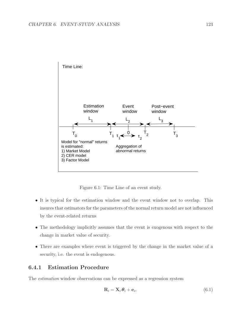
CHAPTER 6. EVENT-STUDY ANALYSIS 123
τ1
Estimationwindow
Eventwindow
Post−eventwindow
T0
T1
T2 T
30
Time Line:
Model for "normal" returnsis estimated:1) Market Model2) CER model3) Factor Model
τ2
Aggregation ofabnormal returns
L1 L
2L
3
Figure 6.1: Time Line of an event study.
• It is typical for the estimation window and the event window not to overlap. This
insures that estimators for the parameters of the normal return model are not influenced
by the event-related returns
• The methodology implicitly assumes that the event is exogenous with respect to the
change in market value of security.
• There are examples where event is triggered by the change in the market value of a
security, i.e. the event is endogenous.
6.4.1 Estimation Procedure
The estimation window observations can be expressed as a regression system
Ri = Xi θi + ei, (6.1)
CHAPTER 6. EVENT-STUDY ANALYSIS 124
where Ri = (Ri,T0+1, . . . , Ri,T1)′ is an L1×1 vector, Xi = ( ι Rm ) is an L1×2 matrix with
a vector of ones in the first column and the vector of market returns observations Rm in
the second column, Rm = (Rm,T0+1, . . . , Rm,T1)′, θi = (αi, βi)
′ is a 2× 1 parameter vector.
One estimates model (6.1) and obtains the OLS estimates θi, σ2ei, ei, Var(θi). The sample
vector of abnormal returns e∗i for firm i from the event window, T1 + 1 to T2, is computed
as follows:
e∗i = R∗i −X∗
i θi,
where R∗i = (Ri,T1+1, . . . , Ri,T2
)′ is an L2×1 vector of event-window returns, X∗i = ( ι R∗
m )
is an L2×2 matrix with a vector of ones in the first column and the vector of market returns
observations R∗m in the second column, R∗
m = (Rm,T1+1, . . . , Rm,T2)′, θi is an OLS estimate.
Conditional on the market return over the event window, the abnormal returns will be
jointly normal with zero mean and conditional covariance matrix Vi which is defined as:
Vi = σ2e
[I+X∗
i (X′i Xi)
−1X∗′i
]. (6.2)
The covariance matrix of abnormal return consists of two parts. The first term is the variance
due to future disturbances and the second term is the additional variance due to the sampling
error in θi.
Under the null hypothesis, H0, that the given event has no impact on the mean or
variance of returns, the vector of event window sample abnormal returns has the following
distribution:
e∗i ∼ N(0, Vi),
where Vi is defined in (6.2).
6.4.2 Aggregation of Abnormal Returns
The abnormal return observations must be aggregated in order to draw overall inferences
for the event of interest. The aggregation is along two dimensions - through time and across
securities.
The aggregation through time:
• To accommodate multiple sampling intervals within the event window one needs to
introduce cumulative abnormal returns (CAR).
CHAPTER 6. EVENT-STUDY ANALYSIS 125
• Define CARi(τ1, τ2) as the cumulative abnormal return for security i from τ1 to τ2
where T1 < τ1 ≤ τ2 ≤ T2.
• Let γ be an L2 × 1 vector of one in positions τ1 − T1 to τ2 − T1 and zeros elsewhere.
• Then, we have
CARi(τ1, τ2) ≡ γ ′ e∗i , and Var[CARi(τ1, τ2)] = σ2i (τ1, τ2) = γ ′ Vi γ.
• Under H0 that the given event has no impact on the mean or variance of returns:
CARi ∼ N(0, σ2
i (τ1, τ2)).
• One can construct a test of H0 for security i as follows:
SCARi(τ1, τ2) =CARi(τ1, τ2)
σi(τ1, τ2), (6.3)
where σ2i (τ1, τ2) is calculated with σ2
e substituted for σ2ei.
• Under the null hypothesis the distribution of SCAR(τ1, τ2) in (6.3) is Student-t with
L1 − 2 degrees of freedom.
The aggregation through time and across securities:
1. The first approach is as follows.
• Assume that there is not any correlation across the abnormal returns of different
securities. This implies that there is not any overlap in the event windows of the
included securities.
• Given a sample of N securities, defining e∗ as the sample average of the N ab-
normal return vectors, one has:
e∗ =1
N
N∑
i=1
e∗i , and Var[e∗] = V =1
N2
N∑
i=1
Vi.
• Define CAR(τ1, τ2), the cumulative average abnormal return, as follows:
CAR(τ1, τ2) ≡ γ ′ e∗, and Var(CAR(τ1, τ2) = σ2(τ1, τ2) = γ ′ Vγ.
CHAPTER 6. EVENT-STUDY ANALYSIS 126
• Under the assumption that the event windows of the N securities do not overlap,
inferences about the cumulative abnormal returns can be drawn using
CAR(τ1, τ2) ∼ N(0, σ2(τ1, τ2)
).
• In practice, σ2(τ1, τ2) is unknown and one needs to use σ2(τ1, τ2) =
1N2
∑Ni=1 σ
2i (τ1, τ2)
as a consistent estimator to test H0 using
J1 =CAR(τ1, τ2)
[σ2(τ1, τ2)]
1
2
−→ N(0, 1).
2. The second approach of aggregation is to give equal weighting to the individual SCARi’s.
• Define
SCAR(τ1, τ2) =1
N
N∑
i=1
SCARi(τ1, τ2).
• Assuming that the event securities of the N securities do not overlap in calendar
time, the null hypothesis H0 can tested using
J2 =
(N(L1 − 4)
L1 − 2
) 1
2
SCAR(τ1, τ2) −→ N(0, 1).
Note that the power of tests J1 and J2 might be similar for most studies and of course,
it depends on the alternative.
Sensitivity to Normal Return Model:
Use of the market model reduces the variance of the abnormal return compared to the
constant-mean-model. This is because
σ2ǫit
= (1− ρ2im) Var[Rit],
where ρim = Corr(Rit, Rmt). (please verify the above formula.) For the constant
mean model Rit = µi + ξit,
σ2ξit
= Var[Rit − µi] = Var[Rit].
Thus σ2ǫit
= (1 − ρ2im) σ2ξit
≤ σ2ξit
because 0 ≤ ρ2im ≤ 1. See the empirical examples in
CLM (p. 163) and Table 4.1.
CHAPTER 6. EVENT-STUDY ANALYSIS 127
Inferences with Clustering:
The basic assumption in the aggregation over securities is that individual securities are
uncorrelated in the cross section. This is the case if the event windows over different
securities do not overlap in calendar time. If they do, the correlation should be taken
into account. One way is to aggregate the individual securities with overlapping event
windows to portfolios, and the apply the above standard event study analysis. Another
way is to analyze without aggregation.
6.4.3 Modifying the Null Hypothesis:
So far the null hypothesis has been that the event has no impact on the behavior of the
return. Either a mean effect or variance effect violates this hypothesis. If we are interested
only in the mean effect, say, the analysis must be expanded to allow for changing variances.
A popular way to do this is to estimate cross-sectional variance at each time point within
the event window.
Var[CAR(τ1, τ2)
]=
1
N2
N∑
i=1
[CARi(τ1, τ2)− CAR(τ1, τ2)
]2,
and
Var[SCAR(τ1, τ2)
]=
1
N2
N∑
i=1
[SCARi(τ1, τ2)− SCAR(τ1, τ2)
]2,
Note that you can find a rationale for these variance estimators and discuss assumptions
behind the validity of these estimators (please verify this, left as an exercise). Using
these variance estimators in J1 and J2 test statistics allows for testing the mean effect under
a possible variance effect.
6.4.4 Nonparametric Tests
The advantage of nonparametric approach is that it is free of specific assumptions concerning
the return distribution. Common and classical nonparametric tests are the sign and rank
tests, which can be found in some statistics books; see, for example, Conover (1999). The
sign test is based on the sign of the abnormal return with assumptions: (1) Independence:
returns are independent across securities, (2) Symmetry: positive and negative returns are
equally likely under the null hypothesis of no event effect.

CHAPTER 6. EVENT-STUDY ANALYSIS 128
Let p = P (CARi = 0), then if the research hypothesis is that there is a positive return
effect of the event the statistical null and alternative hypotheses are H0 : p = 0.5 versus
H1 : p > 0.5. Let N+ be the number of cases with positive returns, and N the total number
of cases, then a statistic based on these information for testing the null hypothesis H0 can
be formulated as
J3 =
(N+
N− 0.5
)N1/2
0.5−→ N(0, 1).
Large values of J3 lead to rejection of H0. Note that you can derive a small sample test for
the null hypothesis. What you need to do is to use the Central Limit Theorem and try to
rationale the asymptotic distribution result of J3. For example, define random variables Yi
such that Yi = 1, if the CARi > 0 and Yi = 0 otherwise. Then N+ =∑N
i=1 Yi.
Note that the weakness of the the sign test is that it may not be well defined if the
(abnormal) return distribution is skewed, i.e. if P (ǫ∗it ≥ 0 |H0) 6= P (ǫ∗it < 0 |H0). A rank
test is one choice which allows non-symmetry. Consider only the case for testing the null
hypothesis that the event day abnormal return is zero. The rank test (Wilcoxon rank sum
test) is as follows: Consider a sample of L2 abnormal returns for each of N securities. Order
the returns from smallest to largest, and let Ki,τ = rank(ǫ∗i,t) be the rank number (i.e. Ki,τ
ranges from 1 to L2). Under the null hypothesis of no event impact the abnormal return
should be just arbitrary random value, and consequently obtain an arbitrary rank position
from 1 to L2. That is each observation should take each rank value equally likely, i.e., with
probability 1/L2. Consequently the expected value of Ki,τ at each time point τ and for each
security i under the null hypothesis is
µK = E[Ki,τ ] =
L2∑
j=1
j P (Ki,τ = j) =1
L2
L2∑
j=1
j =1
2(L2 + 1),
and variance
Var[Ki,τ ] =
L2∑
j=1
(j − µK)2 P (Ki,τ = j).
A test statistic for testing the event day (τ = 0) effect, suggested by Corrado (1989), is
J3 =1
N
N∑
i=1
(Ki,0 −
L2 + 1
2
)/s(L2),
where
s(L2) =
√√√√ 1
L2
T2∑
τ=T1+1
(1
N
N∑
i=1
(Ki,τ −
L2 + 1
2
))2
.
CHAPTER 6. EVENT-STUDY ANALYSIS 129
Under the null hypothesis, J3 → N(0, 1). Typically, nonparametric tests are used in con-
junction with the parametric tests. The R code for implementing the Wilcoxon rank sum
test is wilcox.test().
6.4.5 Cross-Sectional Models
Here the interest is in the magnitude of association between abnormal return and character-
istics specific to the observed event. Let Y be an N × 1 vector of CARs and X be an N ×K
matrix of K − 1 characteristics (The first column is a vector of ones for the intercept term).
Then a cross-sectional (linear) model to explain the magnitudes of CARs is
Y = Xθ + η,
where θ is a K × 1 coefficient vector and η is an N × 1 disturbance vector. OLS estimator
θ = (X′ X)−1 X′Y which is consistent (i.e., θ → θ) if E[X′ η] = 0 (i.e., residuals are not
with the explanatory variables) and
Var[θ]= (X′ X)−1 σ2
η.
Replacing σ2η by its consistent estimator
σ2η =
1
N −Kη′ η,
where η = Y−X θ, makes possible to calculate standard errors of the regression coefficients
and construct t-test to make inference on θ-coefficients.
In financial markets homoscedasticity is a questionable assumption. This is why it is
usually suggested to use White (1980)’s heteroscedasticity consistent (HC) standard errors
of θ-estimates. These are obtained as square roots from the main diagonal of
Var[θ]=
1
N(X′ X)−1
[N∑
i=1
xi x′i η
2i
](X′ X)−1.
These are usually available in most econometric packages or you can compute them by
yourself.
Newey and West (1987, 1994) proposed a more general estimator that is consistent of
both heteroscedasticity and autocorrelation (HAC). In general, this estimator essentially
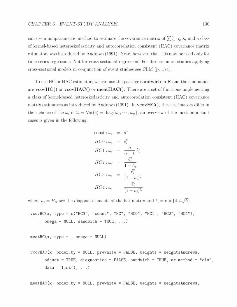
CHAPTER 6. EVENT-STUDY ANALYSIS 130
can use a nonparametric method to estimate the covariance matrix of∑n
t=1 ηt xt and a class
of kernel-based heteroskedasticity and autocorrelation consistent (HAC) covariance matrix
estimators was introduced by Andrews (1991). Note, however, that this may be used only for
time series regression. Not for cross-sectional regression! For discussion on studies applying
cross-sectional models in conjunction of event studies see CLM (p. 174).
To use HC or HAC estimator, we can use the package sandwich in R and the commands
are vcovHC() or vcovHAC() or meatHAC(). There are a set of functions implementing
a class of kernel-based heteroskedasticity and autocorrelation consistent (HAC) covariance
matrix estimators as introduced by Andrews (1991). In vcovHC(), these estimators differ in
their choice of the ωi in Ω = Var(e) = diagω1, · · · , ωn, an overview of the most important
cases is given in the following:
const : ωi = σ2
HC0 : ωi = e2i
HC1 : ωi =n
n− ke2i
HC2 : ωi =e2i
1− hi
HC3 : ωi =e2i
(1− hi)2
HC4 : ωi =e2i
(1− hi)δi
where hi = Hii are the diagonal elements of the hat matrix and δi = min4, hi/h.
vcovHC(x, type = c("HC3", "const", "HC", "HC0", "HC1", "HC2", "HC4"),
omega = NULL, sandwich = TRUE, ...)
meatHC(x, type = , omega = NULL)
vcovHAC(x, order.by = NULL, prewhite = FALSE, weights = weightsAndrews,
adjust = TRUE, diagnostics = FALSE, sandwich = TRUE, ar.method = "ols",
data = list(), ...)
meatHAC(x, order.by = NULL, prewhite = FALSE, weights = weightsAndrews,

CHAPTER 6. EVENT-STUDY ANALYSIS 131
adjust = TRUE, diagnostics = FALSE, ar.method = "ols", data = list())
kernHAC(x, order.by = NULL, prewhite = 1, bw = bwAndrews,
kernel = c("Quadratic Spectral", "Truncated", "Bartlett", "Parzen",
"Tukey-Hanning"), approx = c("AR(1)", "ARMA(1,1)"), adjust = TRUE,
diagnostics = FALSE, sandwich = TRUE, ar.method = "ols", tol = 1e-7,
data = list(), verbose = FALSE, ...)
weightsAndrews(x, order.by = NULL,bw = bwAndrews,
kernel = c("Quadratic Spectral","Truncated","Bartlett","Parzen",
"Tukey-Hanning"), prewhite = 1, ar.method = "ols", tol = 1e-7,
data = list(), verbose = FALSE, ...)
bwAndrews(x,order.by=NULL,kernel=c("Quadratic Spectral", "Truncated",
"Bartlett","Parzen","Tukey-Hanning"), approx=c("AR(1)", "ARMA(1,1)"),
weights = NULL, prewhite = 1, ar.method = "ols", data = list(), ...)
Also, there are a set of functions implementing the Newey and West (1987, 1994) het-
eroskedasticity and autocorrelation consistent (HAC) covariance matrix estimators.
NeweyWest(x, lag = NULL, order.by = NULL, prewhite = TRUE, adjust = FALSE,
diagnostics = FALSE, sandwich = TRUE, ar.method = "ols", data = list(),
verbose = FALSE)
bwNeweyWest(x, order.by = NULL, kernel = c("Bartlett", "Parzen",
"Quadratic Spectral", "Truncated", "Tukey-Hanning"), weights = NULL,
prewhite = 1, ar.method = "ols", data = list(), ...)
For more details, see the papers by Zeileis (2004, 2006).
6.4.6 Power of Tests
The goodness of a statistical test is its ability to detect false null hypothesis. This is called
the power of the test, and is technically measured by power function, which depends on the

CHAPTER 6. EVENT-STUDY ANALYSIS 132
parameter values under the H1 (in the case of abnormal returns, δ)
πα(δ) = Pδ( reject H0 when H0 is not ture),
where α denotes the size of the test (i.e., the significance level which usually is 1% or 5%),
and Pδ(·) denotes the probability as a function of δ. Thus the power function gives the
probability to reject H0 on different values of the tested parameter (δ).
Example:
Consider the J1 test and test the event day abnormal return. Furthermore, assume for
simplicity that the market model parameters are known with σ2A(τ1, τ2) = 0.0016. Then the
power depends on the sample size N , the level of significance α and the magnitude of the
(average) abnormal return δ. For the fixed α = 0.05, the two-sided test, i.e., H0 : δ = 0
vs H1 : δ 6= 0 has the power function π0.05(δ) = Pδ(J1 < −z0.025) + Pδ(J1 > z0.025). The
distribution of J1 depends on δ such that
E[J1] =δ√N
σA(τ1, τ2)= µδ.
Thus J1 → N(µδ, 1). Note that J1 − µδ ∼ N(0, 1). The power function is then π0.05(δ) ≈P (J1 < −z0.025) + P (J1 > z0.025) = Φ(−z0.025 − µδ) + (1 − Φ(z0.025 − µδ)), where z0.025 is
the critical value at 0.025 level and Φ(·) is the cumulative distribution function (CDF) of
the standardized normal distribution, N(0, 1). Below are graphs of the power function of
the J1 test at the 5% significance level for sample sizes 1, 10, 20 and 50. We observe that
the smaller the effect is the larger the sample size must be in order for the test statistic to
detect it. Especially for N = 1 (individual stocks) the effect must be relatively high before
it can be statistically identified. The important factor affecting the power is the parameter
µδ = δ√N/σA, which is a kind of signal-to-noise ratio, where δ is the amount of signal and
σA/√N is the noise component, which decreases as a function of the sample size (number
of events).
6.5 Further Issues
1. Role of the sampling interval: The interval between adjacent observations con-
stitute the sampling interval (minutes, hour, day, week, month). If the event time is
known accurately a shorter sampling interval is expected lead higher ability to identify
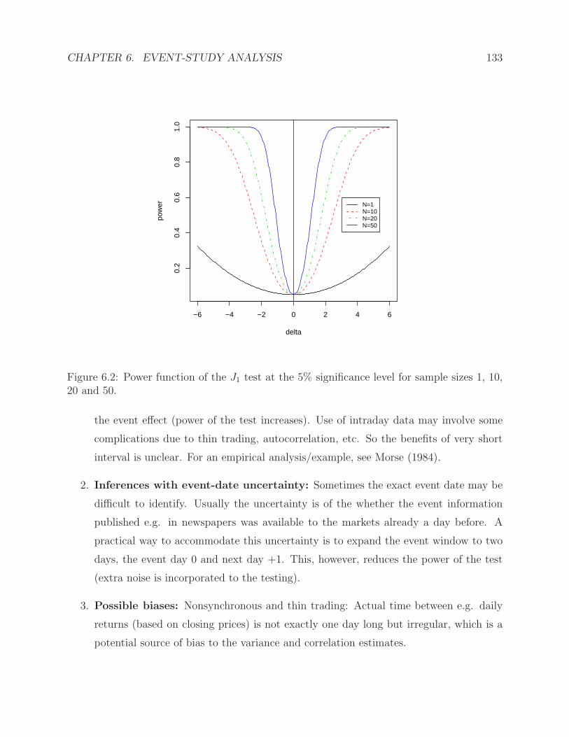
CHAPTER 6. EVENT-STUDY ANALYSIS 133
−6 −4 −2 0 2 4 6
0.2
0.4
0.6
0.8
1.0
delta
pow
er N=1N=10N=20N=50
Figure 6.2: Power function of the J1 test at the 5% significance level for sample sizes 1, 10,20 and 50.
the event effect (power of the test increases). Use of intraday data may involve some
complications due to thin trading, autocorrelation, etc. So the benefits of very short
interval is unclear. For an empirical analysis/example, see Morse (1984).
2. Inferences with event-date uncertainty: Sometimes the exact event date may be
difficult to identify. Usually the uncertainty is of the whether the event information
published e.g. in newspapers was available to the markets already a day before. A
practical way to accommodate this uncertainty is to expand the event window to two
days, the event day 0 and next day +1. This, however, reduces the power of the test
(extra noise is incorporated to the testing).
3. Possible biases: Nonsynchronous and thin trading: Actual time between e.g. daily
returns (based on closing prices) is not exactly one day long but irregular, which is a
potential source of bias to the variance and correlation estimates.
CHAPTER 6. EVENT-STUDY ANALYSIS 134
6.6 Problems
1. In this problem set, you will conduct a small event study which examines the effect
of September 11 terrorist attack on the performance of six companies: Continental
Airlines (CAL), Delta Airlines (DAL), Southwest Airlines(LUV), the Boeing Co. (BA),
Allied Defense Group (ADG), and Engineered Support Systems (EASI)1. To implement
the event study, we will use data for the period 01/01/2001 - 12/01/2001. We will
assume that the event date is September 17 because this the day when the market
reopened. In the analysis, we will examine abnormal returns for the period 20 days
before and 20 days after the event.
Use standardized cumulative abnormal return (SCAR) to test that the event has no
effect on stock prices:
(a) Estimate market model and construct normal returns.
(b) Construct abnormal returns.
(c) Construct cumulative abnormal returns (CAR) for each stock.
(d) Construct standardized cumulative abnormal return for each stock.
Comment your results on each part.
2. Split stocks into two groups. The first group contains airline related stocks (CAL, DAL,
LUV, BA) and the second group contains the stocks of defense oriented companies
(ADG, EASI). Use two approaches discussed in the class and the book by CLM (1997)
to aggregate abnormal stock market returns. Test the null hypothesis that even has no
effect on stock prices. Are results for two groups different? Is it what you expected?
Discuss your results.
3. Read the paper by Bernanke and Kuttner (2005) and write a referee report on this
paper. Think about the possible projects of applying the proposed approaches in this
paper to studying the US stock markets’ reaction to the policy changes by the Federal
Reserve Board.
1 Engineered Support Systems designs, manufactures, and supplies integrated military electronics, supportequipment, and technical and logistics services for all branches of Americas armed forces and certain foreignmilitaries, homeland security forces and selected government and intelligence agencies.
CHAPTER 6. EVENT-STUDY ANALYSIS 135
6.7 References
Andrews, D.W.K. (1991). Heteroskedasticity and autocorrelation consistent covariancematrix estimation. Econometrica, 59, 817-858.
Bernanke, B.S. and K.N. Kuttner (2005). What explains the stock market’s reaction toFederal Reserve policy? Journal of Finance, 60, 1221-1257.
Boehmer, E., J. Musumeci and A. Poulsen (1991). Even study methodology under condi-tions of event induced variance. Journal of Financial Economics, 30, 253-272.
Brown, S. and J. Warner (1980). Measuring security price performance. Journal of Finan-cial Economics, 8, 205-258.
Brown, S. and J. Warner (1985). Using daily stock returns: The case of event studies.Journal of Financial Economics, 14, 3-31.
Campbell, J.Y., A.W. Lo and A.C. MacKinlay (1997). The Econometrics of FinancialMarkets. Princeton University Press, Princeton, NJ. (Chapter 4).
Conover, W.J. (1999). Practical Nonparametric Statistics, 3rd Edition. John Wiley & Sons,New York.
Corrado, C. (1989). A nonparametric test for abnormal security price performance. Journalof Financial Economics, 23, 385-395.
Cochrane, J.H. (2002). The Asset Pricing Theory. Princeton University Press, Prince-ton, NJ.
Dolley, J. (1933). Characteristics and procedure of common stock split-ups. Harvard Busi-ness Review, 316-326.
Fama, E.F. (1991). Efficient capital markets: II. The Journal of Finance, 46, 1599-1603.
Morse, D. (1984). An econometric analysis of the choice of daily versus monthly returns intests of information content. Journal of Accounting Research, 22, 605-623.
Newey, W. and K. West (1987). A simple, positive semi-definite, heteroscedasticity andautocorrelation consistent covariance matrix. Econometrica, 55, 703-708.
Newey, W.K. and K.D. West (1994). Automatic lag selection in covariance matrix estima-tion. Review of Economic Studies, 61, 631-653.
White, H. (1980). A heteroskedasticity-consistent covariance matrix estimators and a directtest for heteroskedasticity. Econometrica, 48, 817-838.
Zeileis, A. (2004). Econometric computing with HC and HAC covariance matrix estimators.Journal of Statistical Software, Volume 11, Issue 10.
Zeileis, A. (2006). Object-oriented computation of sandwich estimators. Journal of Statis-tical Software, 16, 1-16.

Chapter 7
Introduction to Portfolio Theory
7.1 Introduction
Consider the following investment problem.1 One can invest in two non-dividend paying
stocks A and B. Let rA denote monthly return on stock A and rB denote the monthly
return on stock B. Assume that the returns rA and rB are jointly normally distributed with
the following parameters:
µA = E(rA), σ2A = Var(rA), µB = E(rB), σ2
B = Var(rB), and σAB = Cov(rA, rB).
We assume that these values are given (estimated using the historical return data). The
portfolio problem is as follows. An investor has a given amount of wealth and it is assumed
that she will exhaust all her wealth between investment in the two stocks. Let wA denote
the share of wealth invested in stock A and wB denote the share of wealth invested in stock
B, wA + wB = 1. The shares wA and wB are referred to as portfolio weights (allocations).
The long position means that wA > 0 and wB > 0 and the short position is that wA < 0 and
wB > 0. The return on the portfolio over the next period is given by
rp = wA rA + wB rB.
You should be able to show that:
µp = E(rp) = wA µA + wB µB, and σ2p = Var(rp) = w2
A σ2A + w2
B σ2B + 2wAwB σAB.
1This section is mostly from lecture notes of Zivot. For those of you who are interested in more detailson asset allocation, please visit the website of Campbell R. Harvey for the course Global Asset Allocationand Stock Selection at http://www.duke.edu/˜ charvey/Classes/ba453/syl453.htm.
136
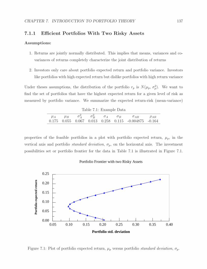
CHAPTER 7. INTRODUCTION TO PORTFOLIO THEORY 137
7.1.1 Efficient Portfolios With Two Risky Assets
Assumptions:
1. Returns are jointly normally distributed. This implies that means, variances and co-
variances of returns completely characterize the joint distribution of returns
2. Investors only care about portfolio expected return and portfolio variance. Investors
like portfolios with high expected return but dislike portfolios with high return variance
Under theses assumptions, the distribution of the portfolio rp is N(µp, σ2p). We want to
find the set of portfolios that have the highest expected return for a given level of risk as
measured by portfolio variance. We summarize the expected return-risk (mean-variance)
Table 7.1: Example Data
µA µB σ2A σ2
B σA σB σAB ρAB
0.175 0.055 0.067 0.013 0.258 0.115 -0.004875 -0.164
properties of the feasible portfolios in a plot with portfolio expected return, µp, in the
vertical axis and portfolio standard deviation, σp, on the horizontal axis. The investment
possibilities set or portfolio frontier for the data in Table 7.1 is illustrated in Figure 7.1.
Portfolio std. deviation
0.05 0.10 0.15 0.20 0.25 0.30 0.35 0.40
Por
tfol
io e
xpec
ted
retu
rn
0.00
0.05
0.10
0.15
0.20
0.25
Portfolio Frontier with two Risky Assets
Figure 7.1: Plot of portfolio expected return, µp versus portfolio standard deviation, σp.

CHAPTER 7. INTRODUCTION TO PORTFOLIO THEORY 138
The portfolio weight on asset A, wA, is varied from −0.4 to 1.4 in increments of 0.1 and
the weight on asset B varies from 1.4 to −0.4, i.e. there are 18 portfolios with weights
(wA, wB) = (−0.4, 1.4), (−0.3, 1.3), . . . , (1.4,−0.4). We compute µp and σp for each of
these portfolios. Portfolio at the bottom of parabola, denoted byM , has the smallest variance
among all feasible portfolios. This portfolio is called global minimum variance portfolio. To
find the minimum variance portfolio one solves the constrained optimization problem
minwA,wB
σ2p = w2
A σ2A + w2
B σ2B + 2wAwB σAB s.t. wA + wB = 1.
Solving this problem, one finds that the weights of stocks A and B for the minimum variance
portfolio are as follows:
wminA =
σ2B − σAB
σ2A + σ2
B − 2σAB
, and wminB = 1− wmin
A .
For our example, using the data in Table 7.1, we get wminA = 0.2 and wmin
B = 0.8. Note that
the shape of investment possibilities is very sensitive to the correlation between assets A and
B.
7.1.2 Efficient Portfolios with One Risky Asset and One Risk-FreeAsset
Continuing with the example, consider an investment in asset B and the risk free asset (for
example, US T-bill rate) and suppose that rf = 0.03. The risk free asset has some special
properties:
µf = E[rf ] = rf , Var(rf ) = 0, and Cov(rB, rf ) = 0.
The portfolio expected return and variance are:
rp = wB rB + (1− wB)rf , µp = wB (µB − rf ) + rf (7.1)
σ2p = w2
Bσ2B. (7.2)
Note that (7.2) implies that wB = σp/σB. Plugging this result into (7.1) and we obtain that
the set of efficient portfolios follows the equation:
µp = rf +µB − rfσB
σp. (7.3)
Therefore, the efficient set of portfolios is a straight line in (µp, σp) with intercept rf and
slope (µB − rf )/σB. The slope of the combination line between risk free asset and a risky
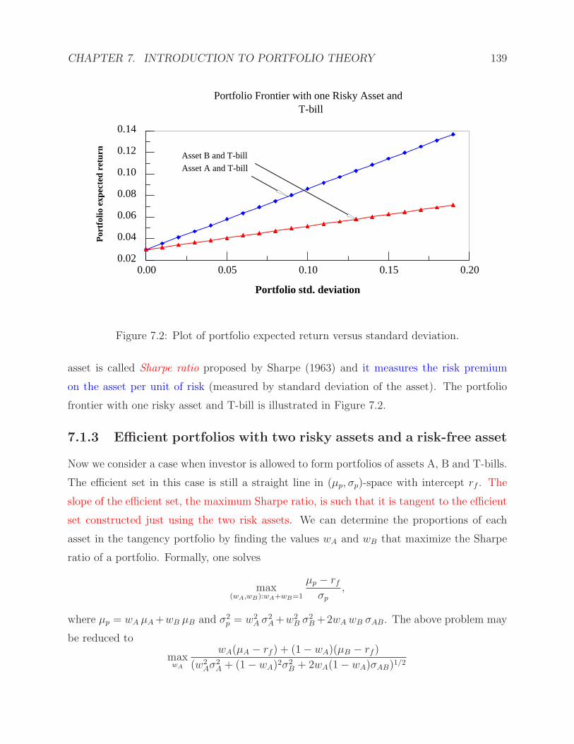
CHAPTER 7. INTRODUCTION TO PORTFOLIO THEORY 139
Portfolio std. deviation
0.00 0.05 0.10 0.15 0.20
Por
tfol
io e
xpec
ted
retu
rn
0.02
0.04
0.06
0.08
0.10
0.12
0.14
Portfolio Frontier with one Risky Asset and T-bill
Asset A and T-bill
Asset B and T-bill
Figure 7.2: Plot of portfolio expected return versus standard deviation.
asset is called Sharpe ratio proposed by Sharpe (1963) and it measures the risk premium
on the asset per unit of risk (measured by standard deviation of the asset). The portfolio
frontier with one risky asset and T-bill is illustrated in Figure 7.2.
7.1.3 Efficient portfolios with two risky assets and a risk-free asset
Now we consider a case when investor is allowed to form portfolios of assets A, B and T-bills.
The efficient set in this case is still a straight line in (µp, σp)-space with intercept rf . The
slope of the efficient set, the maximum Sharpe ratio, is such that it is tangent to the efficient
set constructed just using the two risk assets. We can determine the proportions of each
asset in the tangency portfolio by finding the values wA and wB that maximize the Sharpe
ratio of a portfolio. Formally, one solves
max(wA,wB):wA+wB=1
µp − rfσp
,
where µp = wA µA+wB µB and σ2p = w2
A σ2A+w
2B σ
2B+2wAwB σAB. The above problem may
be reduced to
maxwA
wA(µA − rf ) + (1− wA)(µB − rf )
(w2Aσ
2A + (1− wA)2σ2
B + 2wA(1− wA)σAB)1/2

CHAPTER 7. INTRODUCTION TO PORTFOLIO THEORY 140
Portfolio std. deviation
0.00 0.05 0.10 0.15 0.20 0.25
Por
tfol
io e
xpec
ted
retu
rn
0.00
0.05
0.10
0.15
Portfolio Frontier with two Risky Assets and T-bill
Asset A and T-bill
Asset B and T-bill
Tangency Portfolio
Figure 7.3: Plot of portfolio expected return versus standard deviation.
The solution to this problem is:
wTA =
(µA − rf )σ2B − (µB − rf )σAB
(µA − rf )σ2B + (µB − rf )σ2
A − (µA − rf + µB − rf )σAB
, and wTB = 1− wT
A.
For the example data in Table 7.1 and using rf = 0.03, we get wTA = 0.542 and wT
B = 0.458.
The expected return on the tangency portfolio is µT = 0.11 and σT = 0.124. The portfolio
frontier with two risky assets and T-bill is illustrated in Figure 7.3. The efficient portfolios
are combinations of the tangency portfolio and the T-bill. This important result is known
as the mutual fund separation theorem. Which combination of the tangency portfolio and
the T-bill an investor will choose depends on the investor’s risk preferences. For example, a
highly risk averse investor may choose to put 10% of her wealth in the tangency portfolio
and 90% in the T-bill. For example, a highly risk averse investor may choose to put 10%
of her wealth in the tangency portfolio and 90% in the T-bill. Then she will hold 5.42%
(0.1× 0.542) of her wealth in asset A, 4.58% of her wealth in asset B and 90% of her wealth
in the T-bill.
7.2 Efficient Portfolios with N risky assets
Assume that there be N risky assets with mean vector µ and covariance matrix Ω. Assume
that the expected returns of at least two assets differ and that the covariance matrix is
CHAPTER 7. INTRODUCTION TO PORTFOLIO THEORY 141
of full rank. Define wa as the N × 1 vector of portfolio weights for an arbitrary portfolio
a with weights summing to unity. Portfolio a has mean return µa = w′a µ and variance
σ2a = w′
aΩwa. The covariance between any two portfolios a and b is w′a Ωwb. We consider
minimum-variance portfolios in the absence of a risk free asset.
Definition: Portfolio p is the minimum-variance portfolio of all portfolios with mean return
µp if its portfolio weight is the solution to the following constrained optimization:
minw
w′Ωw : w′µ = µp, and w′ι = 1,
where ι is a conforming vector of ones. To solve this problem, we form a Lagrangian function
L, differentiate with respect to w, set the resulting equations equal to zero, and then solve
for w. For the Lagrangian function we have:
L = w′ Ωw+ 2 δ1 (µp −w′ µ) + 2 δ2 (1−w′ι),
where 2 δ1 and 2 δ2 are Lagrange multipliers. Differentiating L with respect to w we get:
wp = Ω−1(δ1 µ+ δ2 ι). (7.4)
We find Lagrange multipliers from the constraints satisfying(µ′Ω−1µ ι′Ω−1µ
µ′Ω−1ι ι′Ω−1ι
) (δ1δ2
)=
(µp
1
)≡(B AA C
) (δ1δ2
),
where A = ι′Ω−1µ, B = µ′Ω−1µ, and C = ι′Ω−1ι. Hence, with D = BC − A2,
δ1 = (C µp − A)/D, and δ2 = (B − Aµp)/D.
Plugging in to (7.4) we get the portfolio weights and variance:
wp = g+ µp h,
where g = [B(Ω−1ι)−A(Ω−1 µ)]/D and h = [C(Ω−1 µ)−A(Ω−1ι)]/D. There is a number
of results for minimum-variance portfolios (you may refer to CLM for more results):
• Result 1: The minimum-variance frontier can be generated from any two distinct
minimum-variance portfolios
• Result 2: For the global minimum-variance portfolio, g, we have:
wg =1
CΩ−1ι, µg =
A
C, and σ2
g =1
C.
CHAPTER 7. INTRODUCTION TO PORTFOLIO THEORY 142
Given a risk free asset with return rf the minimum-variance portfolio with expected return
µp will be a solution to the constrained optimization:
minw
w′Ωw, s.t. w′µ+ (1−w′ι) rf = µp.
The solution is:
wp =µp − rf
(µ− rf ι)′Ω−1(µ− rf ι)
Ω−1(µ− rf ι).
In this case wp can be expressed as follows:
wp = cp w,
where
cp =µp − rf
(µ− rf ι)′Ω−1(µ− rf ι)
, and w = Ω−1(µ− rf ι).
With a risk free asset all minimum-variance portfolios are a combination of a given risky
asset portfolio with weights proportional to w and the riskfree asset. This portfolio is called
tangency portfolio and has the weight vector:
wq =1
ι′Ω−1(µ− rf ι)Ω−1(µ− rf ι).
The Sharpe ratio for any portfolio a is defined as the mean excess return divided by the
standard deviation of return:
sra = (µa − rf )/σa.
The Sharpe ratio is the slope of the line from the risk free return (rf , 0) to the portfolio
(µa, σa). The tangency portfolio q can be characterized as the portfolio with the maximum
Sharpe ratio of all portfolios of risky assets. Therefore, testing the mean-variance efficiency
of a given portfolio is equivalent to testing whether the Sharpe ratio of the portfolio is the
maximum of the set Sharpe ratios of all possible portfolios.
7.3 Another Look at Mean-Variance Efficiency
Review of the capital asset pricing model (CAPM):
• There is finite number of securities indexed by i, i = 0, . . . , N .
• Let rft denote the risk-free rate at period t.
CHAPTER 7. INTRODUCTION TO PORTFOLIO THEORY 143
• The security 0 is risk-free. It has a price of 1 at date t and its price is 1 + rt at period
t+ 1.
• Other securities are risky and have prices pit, i = 1, . . . , N , t = 1, . . . , T . There are
no dividends.
• A portfolio is described by an allocation vector (w0, w1, . . . , wN)′ = (w0, w
′)′
• An acquisition cost of portfolio at date t is Wt = w0 +w′pt.
• A value of portfolio at date t + 1 is unknown, but its expectation and variance are as
follows:
µWt(w0, w) = Et[Wt+1] = w0(1 + rft) +w′Et[pt+1],
and
η2Wt(w0, w) = Vart(Wt+1) = w′ Vart[pt+1]w.
• The investor’s optimization objective is:
maxw0,w
[µWt
(w0,w)− λ
2η2Wt
(w0,w)
](7.5)
subject to the budget constraint
w0 +w′pt = W, (7.6)
where W is the initial endowment (wealth) at time t and λ is the investor’s risk
aversion. From the budget constraint (7.6), one can derive the quantity of risk-free
asset: w0 = W −w′pt.
• The objective function (7.5) can be rewritten as:
maxw
[W (1 + rft) +w′Et(pt+1)− pt(1 + rft) −
λ
2w′Vart[pt+1]w
],
or
= maxw
[w′µt −
λ
2w′Ωt w
],
where Yt+1 = pt+1 − pt(1 + rft) is an N × 1 vector of the excess gain on risky assets
(excess returns), µt = Et(Yt+1) is the expected mean of excess returns (N × 1 vector),
Ωt = Vart(pt+1) is an N ×N covariance matrix of expected returns.
CHAPTER 7. INTRODUCTION TO PORTFOLIO THEORY 144
The objective function is concave in µ, and the optimal allocation satisfies the first-order
condition:
µt = λΩt w∗t ,
which implies that the solutions of the mean-variance optimization, that is, the mean-
variance efficient portfolio allocations, consist of allocations in risky assets as follows:
w∗t =
1
λΩ−1
t µt. (7.7)
The corresponding quantity of risk-free asset is w∗0,t = W −w∗′
t pt.
7.4 The Black-Litterman Model
7.4.1 Expected Returns
In the traditional mean-variance approach the user inputs a complete set of expected returns
and the variance matrix of expected returns, and then the portfolio optimizer generates
the optimal portfolio weights according to equation (7.7). In the Black-Litterman model
proposed by Black and Litterman (1992), the user inputs
(1) any number of views or statements about the expected returns of arbitrary portfolios,
and
(2) equilibrium values.
The model combines the views, producing both the set of expected returns of assets and
as the optimal portfolio weights. The Black-Litterman (BL) model creates stable, mean-
variance efficient portfolios, which overcomes the problem of input-sensitivity. It provides the
flexibility to combine the market equilibrium with additional market views of the investor.
This model uses “equilibrium” returns that clear the market as a starting point for the
neutral expected returns. The equilibrium returns are derived using a reversed optimization
method:
Π = λΩwmkt, (7.8)
where Π is an N × 1 vector of implied excess equilibrium returns, λ is the risk aversion
coefficient, Ω is a N × N covariance matrix of excess returns, wmkt is the N × 1 vector of
market capitalization weights. The risk aversion coefficient λ measures the rate at which an
investor will forego expected return for less variance. Therefore, the average risk tolerance of
CHAPTER 7. INTRODUCTION TO PORTFOLIO THEORY 145
the world is represented by the risk-aversion parameter λ. The equilibrium expected returns
are Π and the CAPM prior distribution for the expected returns is Π + εe, where εe is
normally distributed with mean zero and covariance τ Σ and the parameter τ is a scalar
measuring the uncertainty of the CAPM prior. As you have seen in the previous section, the
solution to the unconstrained maximization problem: max[w′ µ− λw′ Ωw/2] implies
w =1
λΩ−1 µ, (7.9)
where µ is the expected mean of excess returns. One may use the historical return vector
(µhist) as an estimate of next period return or an estimate of µ using other methods. If
µ = Π, then the optimal weight vector w in (7.9) equals to wmkt. Otherwise, w will not
equal to wmkt.
He and Litterman (1999) cited two problems with the Markowitz framework of Markowitz
(1952):
1. The Markowitz formulation requires expected returns to be specified for every com-
ponent of the relevant universe, while investment managers tend to focus on small
segments of their potential investment universe.
2. When managers try to optimize using the Markowitz approach, they usually find that
portfolio weights (when not overly constrained) to appear to be extreme and not par-
ticularly intuitive. Also, the optimal weights seem to change dramatically from period
to period. This is illustrated in Tables 7.2 and 7.3.
7.4.2 The Black-Litterman Model
The BL formulas for expected returns are written as follows:
E(R) =
(1
τΩ−1 +P′ Σ−1 P
)−1(1
τΩ−1Π+P′Σ−1 Q
)(7.10)
Var(R) =
(1
τΩ−1 +P′Σ−1 P
)−1
, (7.11)
where E(R) is the N ×1 updated (posterior) return vector, τ is scalar, P is a K×N matrix
that identifies the assets involved in the K views, Σ is a K ×K diagonal covariance matrix
of error terms from expressed views, Q is a K × 1 view vector. The expressions for E(R)
and Var(R) are used in formula (7.9) to find optimal weights. The BL model allows investor

CHAPTER 7. INTRODUCTION TO PORTFOLIO THEORY 146
Table 7.2: Expected excess return vectors
Asset Class Historical CAPM GSMI CAPM Implied Equilibriumµhist µGSMI Portfolio µp Return Π
US Bonds 3.15% 0.02% 0.08% 0.08%Int’l Bonds 1.75% 0.18% 0.67% 0.67%US Large Growth -6.39% 5.57% 6.41% 6.41%US Large Value -2.86% 3.39% 4.08% 4.08%US Small Growth -6.75% 6.59% 7.43% 7.43%US Small Value -0.54% 3.16% 3.70% 3.70%Int’l Dev Equity -6.75% 3.92% 4.80% 4.80%Int’l Emerg. Equity -5.26% 5.60% 6.60% 6.60%
Weighted Average -1.97% 2.41% 3.00% 3.00%Standard Deviation 3.73% 2.28% 2.53% 2.53%
High 3.15% 6.59% 7.43% 7.43%Low -6.75% 0.02% 0.08% 0.08%
All four estimates are based on 60 months of excess returns over the risk-free rate.The two CAPM estimates are based on a risk premium of 3. Dividing the riskpremium by the variance of the market (or benchmark) excess returns (σ2) resultsin a risk-aversion coefficient (λ) of approximately 3.07.All the assets show the evidence of fat tails, since the kurtosis exceeds 3, which isthe normal value
Table 7.3: Recommended portfolio weights
Asset Class Weignt based Weight based Weight MarketAsset Class Historical CAPM GSMI based on Capitalization
µhist µGSMI Π wmkt
US Bonds 1144.32% 21.33% 19.34% 19.34%Int’l Bonds -104.59% 5.19% 26.13% 26.13%US Large Growth 54.99% 10.80% 12.09% 12.09%US Large Value -5.29% 10.82% 12.09% 12.09%US Small Growth -60.52% 3.73% 1.34% 1.34%US Small Value 81.47% -0.49% 1.34% 1.34%Int’l Dev Equity -104.36% 17.10% 24.18% 24.18%Int’l Emerg. Equity 14.59% 2.14% 3.49% 3.49%
High 1144.32% 21.33% 26.13% 26.13%Low -104.59% -0.49% 1.34% 1.34%
views to be expressed in either absolute or relative terms. Three sample views may be as
CHAPTER 7. INTRODUCTION TO PORTFOLIO THEORY 147
follows:
View 1: International Developed Equity will have an absolute excess return of 5.25%.
Confidence of view is 25%.
View 2: International Bonds will outperform US Bonds by 25 basis points. Confidence
of view is 50%.
View 3: US Large Growth and US Small Growth will outperform US Large Value
and US Small value by 2%. Confidence of view is 65%.
7.4.3 Building the Inputs
The model does not require that investors specify views on all assets, i.e. K may be less
than N . The uncertainty of the views results in a random, unknown, independent normally-
distributed error term vector e with a mean 0 and covariance matrix Σ, i.e. View is Q + e
and for three views considered Q = (5.25, 0.25, 2). The variance of the error term is Σ =
diagσ1, · · · , σK. The expressed views in column vector Q are matched to specific assets
by matrix P: P = (pij) and for the views considered
P =
0 0 0 0 0 0 1 0−1 1 0 0 0 0 0 00 0 1/2 −1/2 1/2 −1/2 0 0
and the equal weighting scheme in row 3 of P is used. Other options are to use a market
capitalization scheme. Once the matrix P is defined, one can calculate the variance of each
individual view portfolio pk Ωp′k, where pk is kth 1×N row of matrix P. He and Litterman
(1999) assumed that τ = 0.025% and defined:
Σ = τ diagp1 Ωp′1,
. . . , pK Ωp′Kcr.
The process of construction of new combined (or updated) returns may be summarized in
Figure 7.4.
7.5 Estimation of Covariance Matrix
The estimation of the covariance matrix of stock returns is very important in portfolio
selection process. There are two major methods in the literature.

CHAPTER 7. INTRODUCTION TO PORTFOLIO THEORY 148
Risk AversionCoefficient
λ = (ER−rf)/σ2
CovarianceMatrix
(Ω)
MarketCapitalization
Weights(w
mkt)
Views(Q)
Uncertaintyof Views
(Σ)
Implied Equilibrium Return VectorΠ = λ Ω w
mkt
Prior Equilibrium Distributionr~N(Π, τΩ)
View Distributionr~N(Q, Σ)
New Combined Return Distributionr~N(µ, Ψ)
µ = (Ω−1/τ + P’Σ−1P)−1(Ω−1Π/τ +P’Σ−1Q)Ψ = (Ω−1/τ +P’Σ−1P)−1
Figure 7.4: Deriving the new combined return vector E(R).
7.5.1 Estimation Approaches
Let Rt = (r1t, r2t, . . . , rNt)′ be an N × 1 vector of stock returns at period t and R =
1T
∑Tt=1Rt. There are two popular approaches to estimate the covariance matrix of stock
returns:
1. Sample variance-covariance matrix that can be computed as follows:
S =1
T
T∑
t=1
(Rt − R)(Rt − R)′,
where S is an N ×N sample variance-covariance matrix. The main advantage for this
approach is that this estimator does not impose too much structure on the process
generating returns. But, the disadvantage for S is singular if T < N .

CHAPTER 7. INTRODUCTION TO PORTFOLIO THEORY 149
2. Covariance matrix may be computed using factor models of the following form:
rit = αi + βi1 rmt + βi2 f2t + · · ·+ βik fkt + eit, i = 1, ..., N ; t = 1, ..., T, (7.12)
et ∼ N(0, σ2i ) is uncorrelated with the factors. Model (7.12) may be written in matrix
notation as follows:
Rt = α+BXt + Et, t = 1, ..., T, (7.13)
where
B =
β11 · · · β1kβ21 · · · β2k... · · · ...
βN1 · · · βNk
, and Xt =
rmt
f2t...fkt
.
The covariance matrix of returns in model (7.12) can be written as follows:
Φ = (φij) = BΣX B′ + δ, (7.14)
where ΣX is the covariance matrix of factors Xt, δ is a diagonal matrix. Note that
• The factor model (7.12) can be used for risk decomposition of the portfolio. In
particular, the portfolio returns are defined as rp = w′ Rt, where w is an N × 1
vector of weight allocation. The portfolio variance is equal to:
σ2p = w′ Φw = w′ BΣX B′ w+w′ δw,
where w′ BΣX B′ w is the risk attributed to common factors and w′δw is the
risk attributed to the idiosyncratic component.
• For the single index factor model (market model) the covariance matrix (7.14)
becomes:
Φ = σ2m β β′ + δ, (7.15)
where σ2 is the variance of the market factor.
3. The advantages of the factor approach to compute the covariance matrix are that the
covariance matrix Φ is nonsingular and factors may have economic meaning. But the
disadvantages are that there are no consensus on the number of factors to be used in
the model and no consensus on which factors should be included in the model.

CHAPTER 7. INTRODUCTION TO PORTFOLIO THEORY 150
Ledoit and Wolf (2003) suggested using the weighted average of the sample covariance
matrix and the covariance matrix computed based on the single index model as the estimate
of the covariance matrix, i.e. compute the covariance matrix as follows
Sα = αF+ (1− α)S, (7.16)
where 0 ≤ α ≤ 1 and F = (fij) is the estimate of covariance matrix Φ in equation (7.15).
The advantage is that the covariance matrix Sα is nonsingular. and there is no question
about the selection of appropriate factors. The problem with (7.16) is how you choose α.
To choose α, Ledoit and Wolf (2003) proposed a shrinkage method, described next.
7.5.2 Shrinkage estimator of the covariance matrix
Assumptions:
A1: Stock returns are independent and identically distributed (IID) though time.
A2: The number of stocks N is fixed and finite, while the number of observations T goes
to infinity
A3: Stock returns have finite fourth moment.
A4: Φ 6= Σ = Var(Rt) = (σij).
A5: The market portfolio has positive variance, i.e. σ2m > 0.
The actual stocks do not verify Assumption A1 because it ignores:
1. Lead-lags effects.
2. Volatility clustering: autoregressive conditional heteroskedasticity (ARCH).
3. Nonsynchronous trading
Also, note that
1. Any broad-based market index can be used as the market portfolio.
2. Equal-weighted indies are better in explaining stock market variance than value-weighted
indices.
CHAPTER 7. INTRODUCTION TO PORTFOLIO THEORY 151
3. The assumption that residuals are uncorrelated should theoretically preclude that the
portfolio which makes up the market contains any of the N stocks in the sample.
However, as long as the size of the portfolio is large, such a violation will have a small
effect and is typically ignored in applications.
Ledoit and Wolf (2003) suggested that the optimal choice of shrinkage α should satisfy:
α = κ/T, and κ = (π − ρ)/γ,
where π, ρ and γ are appropriately defined. It can be shown from Ledoit and Wolf (2003)
that for the optimal shrinkage constant the following are true:
π =N∑
i=1
N∑
j=1
πij, ρ =N∑
i=1
N∑
j=1
ρij , and γ =N∑
i=1
N∑
j=1
γij,
where πij is the asymptotic variance of T sij, ρij is the asymptotic covariance of√T fij and√
T sij, and γij is (φij−σij)2. Keeping the same notation as in the paper by Ledoit and Wolf
(2003), the consistent estimators for πij, ρij and γij are as follows:
πij =1
T
T∑
t=1
(rit − ri)(rjt − rj)− sij2, ρij =1
T
T∑
t=1
τijt, i 6= j, ρii = πij,
and γij = (fij − sij)2, where
τijt =sj0s00(rit − ri) + si0s00(rjt − rj)− si0sj0(r0t − r0)
s200(r0t − r0)(rit − ri)(rjt − rj)− fiisij
with s200 = σ2m, sj0 = Cov(rj, rm), and r0t = rmt. It can be shown that κ = (π − ρ)/γ is a
consistent estimator for the optimal shrinkage constant κ = (π − ρ)/γ, where
π =N∑
i=1
N∑
j=1
πij, ρ =N∑
i=1
N∑
j=1
ρij, and γ =N∑
i=1
N∑
j=1
γij.
As a result, Ledoit and Wolf (2003) recommended the following shrinkage estimator for the
covariance matrix of stock returns:
Sα = αF+ (1− α)S,
where α = κ/T . For more details about the theory and the methodology, please read the
paper by Ledoit and Wolf (2003).

CHAPTER 7. INTRODUCTION TO PORTFOLIO THEORY 152
7.5.3 Recent Developments
For the recent developments in this area, please read the papers by Ledoit and Wolf (2004)
and Fan, Fan and Lv (2008).
7.6 Problems
1. Read the paper by Fan, Fan and Lv (2008). Write a referee report in which you sum-
marize the main reasons for this paper, the novel approach proposed in the estimation
of variance-covariance matrix, and the main findings.
2. Refer to the paper by Ledoit and Wold (2003) to do this problem. Use the data for
34 stocks in “34stocks.csv” (or other stocks) to find weights in the construction of the
optimal mean-variance portfolio using different approaches. The sample period is from
January, 1985 to September, 2004 with 237 observations. The first column is for the
date of stocks observed and the columns 37-39 contain the information about the name
of companies. If you need the market returns (say, S&P500), please download them
by yourself but the sample period must be the same as that for 34 stocks. You may
use historical sample averages as estimates of expected values of stock returns.
(a) Use the sample variance-covariance matrix of stock returns S to construct the
optimal portfolio.
(b) Use the estimate of variance-covariance matrix of stock returns from the market
model F to construct the optimal portfolio.
(c) Use the improved estimate of variance-covariance matrix of stock returns Sα to
construct the optimal portfolio.
3. Construct the mean-variance efficient frontier for the portfolio of the examined 34
stocks for the last month of the sample. If you need the value for the risk-aversion
coefficient (λ), you can take to it to be as approximately 3. You may use any estimator
of variance-covariance matrix of stock returns. You may use the historical sample
average of stock returns as the estimate of expected value of returns.
4. Download data for returns on 30 Industry Portfolios2 provided by Ken French at
http://mba.tuck.dartmouth.edu/pages/faculty/ken.french/datalibrary.html
2You need to use new specification of industries and monthly returns.

CHAPTER 7. INTRODUCTION TO PORTFOLIO THEORY 153
(a) Use the sample variance-covariance matrix of portfolio returns S to construct the
optimal portfolio consisting of 30 industry portfolios (asset classes).
(b) Use the estimate of variance-covariance matrix of portfolio returns from the mar-
ket model F to construct the optimal portfolio consisting of 30 industry portfolios.
(c) Use the Ledoit and Wolf (2003) or Fan, Fan and Lv (2008)’s estimate of variance-
covariance matrix of stock returns Sα to construct the optimal portfolio consisting
of 30 industry portfolios.
7.7 References
Bevan, A. and K. Winkelmann (1998). Using the Black-Litterman global asset alloca-tion model: Three years of practical experience. Goldman Sachs. The web link ishttp://faculty.fuqua.duke.edu/˜ charvey/Teaching/BA453 2005/GS Using the black.pdf
Black, F. and R. Litterman (1990). Asset allocation: Combining investor views with marketequilibrium. Fixed Income Research, Goldman, Sachs & Co., October.
Black, F. and R. Litterman (1992). Global portfolio optimization. Financial AnalystsJournal, September/October, 28-43.
Campbell, J.Y., A.W. Lo and A.C. MacKinlay (1997). The Econometrics of FinancialMarkets. Princeton University Press, Princeton, NJ. (Chapter 5.2).
Fan, J., Y. Fan and J. Lv (2008). High dimensional covariance matrix estimation using afactor model. Journal of Econometrics, 147, 186-197.
Gourieroux, C. and J. Jasiak (2001). Financial Econometrics: Problems, Models, andMethods. Princeton University Press, Princeton, NJ. (Chapter 3.4, 4.2)
He, G. and R. Litterman (1999). The intuition behind the Black-Litterman model portfo-lios. Investment Management Research, Goldman, Sachs & Co., December. The weblink is
http://faculty.fuqua.duke.edu/˜ charvey/Teaching/BA453 2005/GS The intuition behind.pdf
Idzorek, T.M. (2004). A step-by-step guide to the Black-Litterman model. The web link ishttp://faculty.fuqua.duke.edu/charvey/Teaching/BA453 2005/Idzorek onBL.pdf
Markowitz, H. (1952). Portfolio selection. Journal of Finance, 7, 71-99.
Ledoit, O. and M. Wolf (2003). Improved estimation of the covariance matrix of stockreturns with an application to portfolio selection. Journal of Empirical Finance, 10,603-621.
Ledoit, O. and M. Wolf (2004). A well-conditioned estimator for large-dimensional covari-ance matrices. Journal of Multivariate Analysis, 88, 365-411

CHAPTER 7. INTRODUCTION TO PORTFOLIO THEORY 154
Sharpe, W.F. (1963). A simplified model for portfolio analysis. Management Science, 9,277-293.
Zivot, E. (2002). Lecture Notes on Applied Econometric Modeling in Finance. The weblink is: http://faculty.washington.edu/ezivot/econ483/483notes.htm
Chapter 8
Capital Asset Pricing Model
8.1 Review of the CAPM
Markovitz (1959) laid the groundwork for the capital asset pricing model (CAPM) and cast
the investor’s portfolio selection problem in terms of expected return and variance of return
and argued that investors would optimally hold a mean-variance efficient portfolio, i.e. a
portfolio with the highest expected return for a given level of variance. Sharper (1964)
and Lintner (1965a, 1965b) showed that if investors have homogeneous expectations and
optimally hold mean-variance efficient portfolio then, in the absence of market frictions, the
portfolio of all invested wealth (the market portfolio) will itself be a mean-variance efficient
portfolio.
The Sharper and Lintner version of the CAPM can be expressed in terms of the following
statistical model:
E(Ri) = Rf + βim(E(Rm)−Rf ), βim =Cov(Ri, Rm)
Var(Rm), (8.1)
where Ri is the ith asset return, Rm is the return on the market portfolio, Rf is the return
on the risk-free asset, and stock market returns are assumed to be i.i.d and jointly normally
distributed (CER model). The Sharper-Lintner version can be expressed in terms of excess
returns:
E(Zi) = βimE(Zm), βim =Cov(Zi, Zm)
Var(Zm), (8.2)
where Zi = Ri − Rf and Zm = Rm − Rf . In empirical applications, the estimates of βim
from (8.1) may differ because Rf is stochastic. Notice that model (8.2) may be written as:
E(Zi) =E(Zm)
Var(Zm)Cov(Zi, Zm).
155

CHAPTER 8. CAPITAL ASSET PRICING MODEL 156
There are several derivations of the CAPM model.1 One of the ways to derive the CAPM
model is to assume exponential utility and a normally distributed set of returns. In this case,
the expected utility is
E[u(c)] = E[− exp(−Ac)],
where A is the coefficient of absolute risk aversion and c is consumption. If consumption is
normally distributed, c ∼ N(µc, σ2c ), we have
E[u(c)] = − exp
(−Aµc +
A2
2σ2c
).
Suppose that the investor has initial wealth W which can be split between a risk-free asset
paying Rf and a set of risky assets paying return R which are assumed to be normally
distributed. Let y denote the amount2 of the wealth W invested in each security. Therefore,
the budget constraint is:
c = yf Rf + y′ R, and W = yf + y′ι,
where ι is an N × 1 vector of ones. Then, consumption is normally distributed because
risky assets are normally distributed with the mean µc = yfRf + y′µR and the variance
σ2c = y′Σy, where Σ is an N ×N covariance matrix of risky returns, µR = E(R). Plugging
these equations into utility function, we obtain:
E[u(c)] = − exp
[−A(yf Rf + y′E(R)) +
A2
2y′Σy
],
= − exp
[−AW Rf − Ay′(E(R−Rf ι) +
A2
2y′Σy
], (8.3)
where we use the constraint yf = W − y′ ι. Maximizing (8.3) we obtain the first-order
condition describing the optimal amount to be invested in the risky asset,
−A(E(R)−Rf ι) + A2 Σy = 0,
so that
y =1
AΣ−1[E(R)−Rf ι]. (8.4)
1You may check Chapter 9 of Cochrane (2001) for a rigorous discussion.2Note that this is amount and not a fraction.
CHAPTER 8. CAPITAL ASSET PRICING MODEL 157
Note that the amount of wealth invested in risky assets is independent of the level of wealth.
That is why one usually says that the investor has absolute rather than relative risk aversion.
One may rewrite the equation (8.4) as:
E(R)−Rf ι = AΣy. (8.5)
Note that
Σy = [E(R− µR)(R− µR)′]y = E(R− µR)(y
′(R− µR))′
= E(R− µR)[y′R+ yf Rf − (y′µR + yf Rf )] = Cov(R, Rp),
where Rp = y′R + yf Rf , which is the investor’s overall portfolio. Therefore, Σy gives the
covariance of each return with the investor’s overall portfolio. If all investors are identical,
then the market portfolio is the same as the individual’s portfolio so Σy also gives the
covariance of each return with Rm, i.e Σy = Cov(R, Rm). Equation (8.5) then becomes:
E(R)−Rf ι = ACov(R, Rm). (8.6)
Note that equation (8.1) may be written as:
E(R)−Rf ι = Cov(R, Rm)
[E(Rm)−Rf
Var(Rm)
],
which is the same as the model given in (8.2). Therefore, this derivation of CAPM ties the
market price of risk to the risk aversion coefficient. This can also be seen by applying (8.6)
to the market return itself:
E(Rm)−Rf = AVar(Rm).
8.2 Statistical Framework for Estimation and Testing
Define Zt as an N × 1 vector of excess returns for N assets (or portfolios of assets). For
these N assets, the excess returns can be described using the excess-return market model:
Zt = α+ β Zmt + et, E(et) = 0, E(et e′t) = Σ, Cov(Zmt, et) = 0,
where β is the N × 1 vector of betas, Zmt is the time period t market portfolio excess
return, and α and et are N × 1 vectors of asset return intercepts and disturbances. Denote
E(Zmt) = µm and E(Zmt−µm)2 = σ2
m. Three implications of Sharper-Lintner version of the
CAPM:

CHAPTER 8. CAPITAL ASSET PRICING MODEL 158
1. The vector of asset return intercepts is zero. The regression intercepts may be viewed
as the pricing errors.
2. The cross-sectional variation of expected excess returns is entirely captured by betas.
3. The market risk premium, E(Zmt), is positive.
There are three major methods of estimating the parameters: time series, cross-sectional,
and Fama-MacBeth, described next.
8.2.1 Time-Series Regression
The implication of the Sharper-Lintner version of the CAPM that the regression intercepts
of excess returns model are zero may be tested using time-series regressions. One runs N
time-series regressions:
Zit = αi + βim Zmt + eit, i = 1, . . . , N.
The estimate of the factor premium (market premium), λ = E(Zm), may be found as the
sample mean of the factor:
λ =1
T
T∑
t=1
Zmt.
For the case of uncorrelated and homoskedastic regression errors one may use the standard
t-tests to check that the pricing errors αi, i = 1, ..., N , are in fact zero. However, one usually
wants to know whether all the pricing errors are jointly equal to zero. This hypothesis can
be tested using the following Wald-type χ2 test3:
T
[1 +
(µm
σm
)2]−1
α′ Σ
−1α ∼ χ2
N ,
where Σ is the residual covariance matrix, i.e. the sample estimate of E(et e′t) = Σ. This
test is valid asymptotically, i.e as T → ∞, and does not require the assumption of no
autocorrelation or heteroskedasticity. A finite-sample F -test for the hypothesis that a set of
parameters are jointly zero:
T −N − 1
N
[1 +
(µm
σm
)2]−1
α′ Σ
−1α ∼ FN,T−N−1.
3You may check Chapter 5.3 of CLM (1997) and Chapter 12 of Cochrane (2001) for a rigorous discussion.

CHAPTER 8. CAPITAL ASSET PRICING MODEL 159
This distribution requires that the errors are normal as well as uncorrelated and homoskedas-
tic. Note that the assumption of uncorrelated residuals is needed to make sure that Σ is
non-singular. See CLM (1997, p.193) for details.
If there are many factors that are excess returns, the same ideas work. The regression
equation is
Zit = αi + β′i ft + eit,
where ft is a K × 1 vector of excess returns, βi is a K × 1 vector of factor loadings. The
asset pricing model has the following form:
E(Zit) = β′iE(ft).
We can estimate α and β with ordinary least squares (OLS) time-series regressions. Assum-
ing normal i.i.d. errors with constant variance, one may use the following test statistic:
T −N −K
N
[1 + µ
′fΩ
−1
f µf
]−1
α′ Σ
−1α ∼ FN,T−N−K ,
where N is the number of assets, K is the number of factors and Ωf = 1T
∑Tt=1(ft − µf )(ft −
µf )′. Cochrane (2001, p.234) showed that the asymptotic χ2 test
T[1 + µ
′fΩ
−1
f µf
]−1
α′ Σ
−1α ∼ χ2
N .
does not require the assumption of i.i.d errors or independence from factors.
8.2.2 Cross-Sectional Regression
The central economic question is why average returns vary across assets. For the excess
returns model of Sharper and Lintner (see (8.2)), we have
E(Zi) = βim λ,
where E(Zm) = λ is the factor risk premium. This model states that the expected returns
of an asset should be high if that asset has high betas or a large risk exposure to factor(s)
that carry high risk premia. This is illustrated in Figure 8.1. The model says that average
returns should be proportional to betas. However, even if the model is true, it will not work
out perfectly in each sample, so there will be some spread αi as shown. Given these facts,
a natural idea is to run a cross-sectional regression to fit a line through the scatter plot of
Figure 8.1. Cross-sectional regressions consist of two steps:
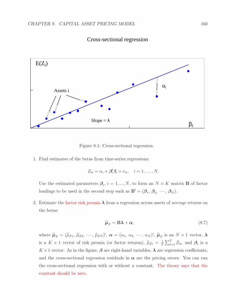
CHAPTER 8. CAPITAL ASSET PRICING MODEL 160
Cross-sectional regression
Assets iαi
βi
E(Zi)
Slope = λ
Figure 8.1: Cross-sectional regression.
1. Find estimates of the betas from time-series regressions:
Zit = αi + β′i ft + eit, i = 1, . . . , N.
Use the estimated parameters βi, i = 1, ..., N , to form an N ×K matrix B of factor
loadings to be used in the second step such as B′ = (β1, β2, · · · , βN).
2. Estimate the factor risk premia λ from a regression across assets of average returns on
the betas:
µZ = Bλ+α, (8.7)
where µZ = (µZ1, µZ2, · · · , µZN)′, α = (α1, α2, · · · , αN)
′, µZ is an N × 1 vector, λ
is a K × 1 vector of risk premia (or factor returns), µZi = 1T
∑Tt=1 Zit, and βi is a
K×1 vector. As in the figure, β are right-hand variables, λ are regression coefficients,
and the cross-sectional regression residuals in α are the pricing errors. You can run
the cross-sectional regression with or without a constant. The theory says that the
constant should be zero.
CHAPTER 8. CAPITAL ASSET PRICING MODEL 161
OLS Cross-Sectional Regression
Consider a model with only factor without intercept in the cross-sectional regression. OLS
cross-sectional estimates are:
λ = (B′ B)−1B′ µZ , and α = µZ −B λ =[I−B(B′ B)−1 B′] µZ ,
where the true errors are i.i.d over time and independent of the factors. Since the αi are just
time series averages of the true eit, the errors in the cross-sectional regression have covariance
matrix E(αα′) = 1TΣ. Then,
Var(λ) =1
T(B′ B)−1 B′ ΣB (B′ B)−1,
and
Var(α) =1
T(I−B (B′ B)−1B′)Σ (I−B (B′ B)−1 B′).
We could test whether all pricing errors are zero with the statistics:
α′ Var(α)−1 α ∼ χ2
N−K . (8.8)
Note that the asymptotic distribution in (8.8) is χ2N−K but not χ2
N because the covariance
matrix is singular and one has to use a generalized inverse.
GLS Cross-Sectional Regression
Generalized least squares (GLS) cross-sectional estimates are:
λ = (B′ Σ−1
B)−1 BΣ−1µZ , and α = µZ −B λ.
The variance of these estimates is as follows:
Var(λ) =1
T(B′ Σ−1 B)−1, and Var(α) =
1
T(Σ−B (B′Σ−1 B)−1 B′).
One could use the test in (8.8)
α′ Var(α)−1 α ∼ χ2
N−K ,
or use an equivalent test that does not require a generalized inverse:
T α′ Σ
−1α ∼ χ2
N−K . (8.9)
For details, see Cochrane (2001, p.238).
CHAPTER 8. CAPITAL ASSET PRICING MODEL 162
Correction for the Fact that B are Estimated
In applying standard OLS and GLS formulas to a cross-sectional regression, we assume
that the right-hand variables B are fixed. This is not true since the B in cross sectional
regression are not fixed but are estimated in the time-series regressions. The correction for
the estimation of B is due to Shanken (1992):
Var(λOLS) =1
T[(B ′B )−1B ′ΣB (B ′B )−1(1 + λ′ Σ−1
f λ) +Σf ]
Var(λGLS) =1
T[(B ′Σ−1B )−1(1 + λ′Σ−1
f λ) +Σf ]
Var(αGLS) =1
T(I−B (B ′B )−1B ′)Σ(I−B (B ′B )−1B ′)× (1 + λ′ Σ−1
f λ)
Var(αOLS) =1
T(Σ−B (B ′Σ−1B )−1B ′)(1 + λ′ Σ−1
f λ)
One can use the test (8.8) with corrected estimates of the variances. One can also use the
test in (8.9) for the corrected GLS estimates:
T (1 + λ′GLS Σ
−1
f λGLS) α′GLS Σ
−1αGLS ∼ χ2
N−K . (8.10)
For details, see Cochrane (2001, p.239).
Time Series versus Cross Section
The main difference between cross-sectional and time series regression is that one can run
the cross-sectional regression when the factor is not a return. The time series test requires
factors that are also returns, so that you can estimate factor risk premia by λ = 1T
∑Tt=1 ft.
If the factor is an excess return, the GLS cross-sectional regression, including the factor as
a test asset, is identical to the time-series regression.
8.2.3 Fama-MacBeth Procedure
Fama and MacBeth (1973) suggested an alternative procedure for running cross-sectional
regressions, and for producing standard errors and test statistics. This procedure is widely
used in practice and consists of two steps.
1. Find beta estimates with a time-series regression.
2. Instead of estimating a single cross-sectional regression with the sample averages, by
assuming knowing β’s, we now run a cross-sectional regression at each time period, i.e.
Zit = αt + β′i λt + eit, t = 1, . . . , T.
CHAPTER 8. CAPITAL ASSET PRICING MODEL 163
Then, Fama and MacBeth (1973) suggested that one estimates λ and α as the average of
the cross-sectional regression estimates:
λ =1
T
T∑
t=1
λt, and α =1
T
T∑
t=1
αt.
One can use the standard deviations of the cross-sectional regression estimates to generate
sampling errors for these estimates
Cov(λ) =1
T 2
T∑
t=1
(λt − λ)(λt − λ)′, and Cov(α) =1
T 2
T∑
t=1
(αt − α)(αt − α)′.
It is 1/T 2 because we are finding standard errors of sample means, σ2/T . To test whether
all the pricing errors are jointly zero one can use the χ2 test (or t-test) that we have used
before
α′ Cov(α)−1 α ∼ χ2
N−K ,
where K = 1. Fama and MacBeth (1973) used the variation in the statistic λt over time to
deduce its variation across samples. For mode details, see Chapter 12 of Cochrane (2001,
p.244-p.246) and CLM (1997, p.215-p.216).
8.3 Empirical Results on CAPM
8.3.1 Testing CAPM Based On Cross-Sectional Regressions
The early evidence on testing CAPM was largely positive reporting the evidence consistent
with the mean-variance efficiency of the market portfolio which implies that (a) expected
returns on securities are a positive linear function of their market βs and (b) market βs
suffice to describe the cross-section of expected returns. However, less favorable evidence
for the CAPM started to appear in the so-called anomalies literature. The anomalies liter-
ature shows that contrary to the prediction of the CAPM, the firm characteristics provide
explanatory power for the cross section of average returns beyond the betas of CAPM. This
literature documents several deviations from the CAPM that are related to the following
variables:
1. Size: market equity (ME) adds to the explanation of the cross-section of average
returns.
2. Earnings yield effect.

CHAPTER 8. CAPITAL ASSET PRICING MODEL 164
3. Leverage.
4. The ratio of a firm’s book value of equity to its market value (BE/ME or B/M).
5. The ratio of earning to price (E/P).
We will consider how the cross-sectional regressions are used in practice to test CAPM by
looking at the paper of Fama and French (1992), denoted by FF, and at the paper of Kothari,
Shanken and Sloan (1995), denoted by KSS (1995).
The FF’s findings can be summarized as follows:
1. There is only a weak positive relation between average return and beta over the period
1941-1990. There is virtually no relation over 1963 -1990.
2. Firm size and B/M ratio do a good job of capturing cross-sectional variation in average
returns over 1963-1990. Moreover, the combination of size and B/M ratio seems to
absorb the roles of leverage and E/P ratio in average stock returns
The goal of KSS (1995) is as follows:
1. Re-estimate betas to see whether betas can explain cross-section variation over 1941-
1990 and 1926-1990 using a different data set.
2. Examine whether B/M captures cross-sectional variation in average returns over 1947
-1987.
The analysis of KSS (1995) is done using cross-sectional regressions of average monthly
returns on annual betas. The KSS (1995)’s findings may be summarized as follows:
1. There is substantial ex post compensation for beta risk over 1941-1990 and even more
so over 1927-1990. Estimated risk premium for different portfolio aggregations range
6.2− 11.7%.
2. Using an alternative data source, S&P industry level data, KSS (1995) found that B/M
ratio has a weaker effect on the returns than that in FF.
3. Size, as well as beta, is needed to account for the cross-section of expected returns.
CHAPTER 8. CAPITAL ASSET PRICING MODEL 165
8.3.2 Return-Measurement Interval and Beta
KSS (1995) used the annual data to estimate the market betas unlike FF who used return
data for the beta estimation. KSS (1995) argued that there are at least three reasons longer
measurement-interval returns:
1. CAPM does not provide guidance on the choice of horizon.
2. Beta estimates are biased due to trading frictions and non-synchronous trading or other
phenomena. These biases are mitigated by using longer interval return observations.
3. There appears to be a significant seasonal component to monthly return. Annual return
data is one of the ways to avoid statistical complications that arise from seasonality in
returns.
8.3.3 Results of FF and KSS
KSS (1995) presented the results of cross-sectional regressions for a variety of portfolio ag-
gregation procedures:
• Grouping on beta alone.
• Grouping on size alone.
• Taking intersections of independent beta or size groupings.
• Ranking first on beta and then on size within each beta group.
• Ranking first on size and then on beta.
Note that to form portfolios KSS (1995) estimated beta using the monthly return data over
2 or 5 years. The annual time-series of post-ranked beta-size ranked portfolios are then used
to re-estimate the full-period post-ranking betas for use in cross-sectional regressions. The
cross-sectional model:
Rpt = γ0t + γ1tβp + γ2tSizept−1 + ept, (8.11)
where Rpt the equally weighted (can be value-weighted) buy-and-hold return on portfolio p
from month t; βp is the full-period post-ranking beta of portfolio p, Sizept−1 is the natural
log of the average market capitalization on June 30 of year t of the stocks in portfolio p,
γ0t, γ1t and γ2t are regression parameters; ept is the regression error. FF also included other

CHAPTER 8. CAPITAL ASSET PRICING MODEL 166
variables in cross-sectional regression (8.11). In particular, FF included leverage, E/P, B/M.
The estimation of models in (8.11) is known as “horse race” because it allows to test
whether one set of factors drives out another. For example, we want to know, given market
betas βp, do we need Size factor to price assets, i.e. is γ2t = 0. Obviously, one can use the
asymptotic covariance matrix for γ0t, γ1t, γ2t (by using the improved method by Ledoit and
Wolf (2003)) to form the standard t-test. Note also that γjt in (8.11) ask whether factor j
helps to price assets given the other factors, γjt gives the multiple regression coefficient of
Rpt on factor j given the other factors. Risk premium λj asks whether factor j is priced.
Results: See Tables I, II, III, IV, and V from FF and Tables I, II, and III from KSS
(1995).
The conclusion of KSS (1995) is that beta continues to dominate for size-ranked portfolios.
Then KSS (1995) analyzed selection biases and how it may affect the results from B/M factor.
The intuition is that many firms with high B/M values in 1973 went bankrupt before 1978
and therefore were not included in the COMPUSTAT database. Only the firm with high
B/M that did unexpectedly well were included in the database. As a result, it may have
created the selection bias and affected the effect of B/M factor.
8.4 Problems
1. Download the monthly data for 34 stock prices in the file “34stocks.csv”. Estimate
the single index model for all stocks in the file “34stocks.csv”. You can download the
market returns (say, S&P500 index return) by yourself but the sample period must be
the same as that for 34 stocks in the file.
(a) Use time-series regressions to test the validity of CAPM model for all stocks
simultaneously and individually.
(b) For each stock, present the estimates of market beta and the proportion of risk at-
tributed to the systematic risk. What can you say about the relationship between
the stock systematic risk and stock beta?
CHAPTER 8. CAPITAL ASSET PRICING MODEL 167
(c) For each stock, present the estimates of market beta and average sample returns.
What can you say about the relationship between average stock returns and their
market betas?
(d) Sort your stocks according to the estimates of market beta. Split your stock
into three portfolios containing approximately equal number of stocks. In the
first portfolio you should collect stocks with the low beta, in the second portfolio
collect stocks with the medium beta, and in the third portfolio collect stocks
with the highest beta. This way, you will create a portfolio of low beta stocks, a
portfolio of medium beta stocks, a portfolio of high beta stocks.
(e) Compute the equal-weighted portfolio returns for the constructed portfolios.
(f) Estimate the portfolio market betas. What can you say about the relationship
between average portfolio returns and portfolio betas?
(g) Run Fama-MacBeth cross-sectional regressions for the constructed portfolios and
test for the validity of CAPM model.
8.5 References
Campbell, J.Y., A.W. Lo and A.C. MacKinlay (1997). The Econometrics of FinancialMarkets. Princeton University Press, Princeton, NJ. (Chapter 5).
Chan, L.K.C., J. Karceski and J. Lakonishok (1998). The risk and return from factors.Journal of Financial and Quantitative Analysis, 33, 159-88.
Chan, L.K.C., J. Karceski and J. Lakonishok (1999). On portfolio optimization: Forecastingcovariances and choosing the risk model. Review of Financial Studies, 12 937-74.
Cochrane, J.H. (2001). Asset pricing. Princeton University Press, Princeton, NJ. (Chapters9 and 12)
Davis, J.L., E.F. Fama and K.R. French (2000). Characteristics, covariances, and averagereturns: 1929 to 1997. Journal of Finance, 55, 389-406.
Fama, E.F. and K.R. French (1992). The cross-section of expected stock returns. TheJournal of Finance, 47, 427-465.
Fama, E.F. and K.R. French (1998). Value versus growth: The international evidence.Journal of Finance, 53, 1975-99.
Fama, E.F. and J. MacBeth (1973). Risk, return, and equilibrium: Empirical tests. Journalof Political Economy, 71, 607-636.
CHAPTER 8. CAPITAL ASSET PRICING MODEL 168
Gourieroux, C. and J. Jasiak (2001). Financial Econometrics: Problems, Models, andMethods. Princeton University Press, Princeton, NJ. (Chapters 3-4)
Kothari, S.P., J. Shanken and R.G. Sloan (1995). Another look at the cross-section ofexpected stock returns. The Journal of Finance, 50, 185-224.
Liew, J. and M. Vassalou (2000). Can book-to-market, size and momentum be risk factorsthat predict economic growth? Journal of Financial Economics, 57, 221-245.
Lintner, J. (1965a). Security prices, risk and maximal gains from diversification. Journalof Finance, 20, 587-615.
Lintner, J. (1965b). The valuation of risky assets and the selection risky investments instock portfolios and capital budgets. Review of Economics and Statistics, 47, 163-196.
Markowitz, H. (1959). Portfolio Selection: Efficient Diversification of Investments. JohnWiley, New York.
Shanken, J. (1992). On the estimation of Bets-pricing models. Review of Financial Studies,5, 1-34.
Sharper, W. (1964). capital asset prices: A theory of market equilibrium under conditionsof risk. Journal of Finance, 19, 425-442.
Chapter 9
Multifactor Pricing Models
9.1 Introduction
We have discussed the papers by Fama and French (1992, denoted by FF, here after) and
Kothari, Shanken and Sloan (1995) who showed that CAPM model (single factor model)
does not completely explain the cross section of expected returns and that some additional
factors may be needed to explain the dynamics of expected returns. Two main theoretical
approaches exist to allow for multiple risk factors: arbitrage pricing theory (APT) and inter-
temporal capital asset pricing model (ICAPM). APT is based on arbitrage arguments and
ICAPM is based on equilibrium arguments.
9.1.1 Why Do We Expect Multiple Factors?
The CAPM simplifies matters by assuming that the average investor only cares about the
performance of his/her portfolio. This is not true in practice since the average investor has a
job. Investors are hurt during recessions because some of the investors loose jobs while others
may have lower income (lower salaries). As a result, most investors may prefer the stocks
that do well in recessions, i.e. “counter-cyclical” stocks. Therefore, “pro-cyclical” stocks
that do well during expansion and worse during recessions will have to offer higher average
returns than “counter-cyclical” stocks that do well in recessions. This leads Cochrane (1999)
to conclude that we may expect another dimension of risk arising from covariation with
recessions, “bad times”, that will matter for explaining the average returns.
Empirically useful multifactor asset pricing models include more direct measure of “good
times” or “bad times”:
1. The market return.
169
CHAPTER 9. MULTIFACTOR PRICING MODELS 170
2. Events such as recessions or macroeconomic factors that drive investor’s non-investment
sources of income.
3. Variables such as the D/P ratio or yield curve that forecast stock or bond returns,
so-called “state variables for changing investment opportunity sets”.
4. Returns on other well-diversified portfolios. These portfolios are called factor-mimicking
portfolios. They can be constructed as the fitted value of a regression of any pricing
factor on the set of all asset returns. This portfolio carries exactly the same pricing
information as the original factor.
Note that it is important from theoretical point of view that the extra factors affect the
average investor.
9.1.2 The Model
The Arbitrage Pricing Theory provides an approximate relation for expected asset returns
with an unknown number of unidentified factors. The APT assumes that markets are compet-
itive and frictionless and that the return generating process for asset returns being considered
is:
Rit −Rft = ci + βim(Rmt −Rf
t ) + βiAFAt + βiBFBt + ...+ eit, 1 ≤ i ≤ N, 1 ≤ t ≤ T. (9.1)
Therefore, multifactor models use a time-series multiple regression to quantify an asset’s
tendency to move with multiple risk factors FA, FB1, etc. The equation (9.1) can be written
as follows:
Rit = ci + b′i Ft + eit, E(eit |Ft) = 0, E(e2it) = σ2
i <∞, 1 ≤ i ≤ N, 1 ≤ t ≤ T,
where Rit is the return for asset i at period t, ci is the intercept of the factor model, bi is a
K×1 vector of factor loadings for asset i, Ft is a K×1 vector of common factor realizations,
and eit is the disturbance term. For the system of N assets the model is written as:
Rt = c+BFt + et, E(et |Ft) = 0, E(et e′) = Σ, 1 ≤ t ≤ T,
1Note that APT does not specify that one of the factors should be excess market returns but it is usuallyassumed that one of the factors is excess market returns
CHAPTER 9. MULTIFACTOR PRICING MODELS 171
where Rt is an N × 1 vector with Rt = (R1t, R2t, · · · , RNt)′, c is an N × 1 vector with
c = (c1, c2, · · · , cN)′, B is an N ×K matrix with B = (b1, b2, · · · , bN)′. It is also assumed
that the disturbance term for large well-diversified portfolios vanishes.
Given this structure, Ross (1976) showed that the absence of arbitrage in large economies
implies that:
µ ≈ λ0 ι+BλK ,
where µ is the N × 1 expected return vector, λ0 is the model zero-beta parameter and is
equal to a riskfree return if such an asset exists, and λK is a K × 1 vector of factor risk
premia. Exact factor pricing can be derived from an intertemporal asset pricing framework.
We will analyze models where we have exact factor pricing and will not differentiate the
APT from ICAPM. Therefore,
µ = λ0 ι+BλK .
The multifactor models specify neither the number of factors nor the identification of the
factors. Therefore, to estimate and test the model, we need to determine the factors which
may be observed and unobserved.
9.2 Selection of Factors
There are two approaches to specify the factors: statistical and theoretical.
9.2.1 Theoretical Approaches
Theoretically based approaches fall into two main categories. One approach is to specify
macroeconomic and financial market variables that are thought to capture the systematic
risks of the economy. A second approach is to specify characteristics of firms which are likely
to explain differential sensitivity to the systematic risks and then form portfolio of stocks
based on the characteristics.
9.2.2 Small and Value/Growth Stocks
“Small Cap”, “Large Cap”, “Value”, “Growth” stocks are the names that often used in
finance industry. “Small cap” stocks have small market values (price times shares outstand-
ing). “Value” stocks or “high book/market” stocks have market values that are small relative
to accountant’s book value. Recall that FF (1993) group stocks in portfolios according to
CHAPTER 9. MULTIFACTOR PRICING MODELS 172
size and B/M variables and show that both categories of stocks, “Small Cap” and “Value”,
have relatively high average returns. “Large Cap” and “Growth” stocks are the opposite
and seem to have unusually low average returns.
To explain the difference between stocks related to size and B/M, FF (1993) advocated
a three factor model with the market return, the return on small less big stocks (SMB)
portfolio, and the returns of high B/M less low B/M stocks (HML) portfolio. These three
factors seem to explain cross-sectional variation in average returns for 25 size and B/M
portfolios. FF (1995) argued that the size and value factors are related to the profitability or
financial distress of a firm. Cochrane (1999) noted that one cannot count the “distress” of the
individual firm as a “risk factor” because such distress is idiosyncratic and can be diversified
away. However, the typical investor is an owner of small business and an investor’s income
may be sensitive to the kinds of financial distress among small and distressed value firms.
Therefore, the typical investor would demand a big premium to hold value stocks instead of
growth stocks at low premium.
9.2.3 Macroeconomic Factors
Researchers look at labor income, industrial production, inflation, investment growth as
possible other factors that explain cross section of returns. The factors are easier to motivate
from theoretical point of view but are not as successful as size and value factors of Fama
and French (1993).
Momentum Factor
There is evidence of momentum effect which states that the stocks with the higher average
returns (winners) during the most recent 12 month (excluding the most recent month) con-
tinue to win, i.e. to earn relatively average returns, than the stocks with low returns (losers).
The three factor model of FF (1993) can not explain this phenomena.
Note that even though the model of FF can not explain the momentum phenomena, it
can explain reversal phenomena.
Multifactor Model of FF (1993)
FF (1993) identified five common risk factors in the returns on stocks and bonds:
CHAPTER 9. MULTIFACTOR PRICING MODELS 173
1. Stock-market risk factors
(a) A market factor
(b) A factor related to size, so-called size factor
(c) A factor related to B/M, so-called value factor
2. Bond-market risk factors
(a) Term spread: a factor that should capture unexpected changes in interest rates
(b) Default spread: a factor that should capture the shifts in economic conditions
that change the likelihood of default
The paper by Fama (1993) extended the paper by French and Fama (1992) in several ways:
1. The set of asset returns is expanded. FF (1993) analyzed stock returns as well as bond
returns while FF (1992) analyzed only stock returns.
2. The set of possible factors that may explain the stock returns is expanded. FF (1993)
analyzed the effect of bond market risk factors on stock returns.
3. Different econometric approach is used. FF (1993) used time-series approach while
FF(1992) used cross-sectional approach. To make the use of time-series approach
possible FF constructed factor mimicking portfolios.
Construction of the Explanatory Variables for the Time-Series Regressions
Bond-market factors are constructed as follows:
• Term spread factor. TERM = monthly long-term government bond return minus one-
month Treasury bill rate
• Default factor. DEF = monthly return on a market portfolio of long-term corporate
bonds minus the long-term government bond return
Construction of market factor is easy. It is simply the excess return on market portfolio.
Construction of factor mimicking portfolios that are meant to capture the size effect and
B/M effect is more involved and consists of two steps:

CHAPTER 9. MULTIFACTOR PRICING MODELS 174
1. Construct six size-B/M portfolios. To construct six size-B/M one ranks NYSE stocks
on market capitalization. The median NYSE size is then used to split NYSE, Amex
and NASDAQ stocks into two groups, small and big (S and B). Then rank NYSE
stocks on B/M ratio and compute the breakpoints for the bottom 30% (Low), middle
40% (Medium), and top 30% (High) of the ranked B/M values. Then split all NYSE,
Amex, NASDAQ stocks intro three B/M portfolios. Construct six portfolios (S/L,
S/M, S/H, B/L, B/M, B/H) from intersection of the two market capitalization and
three B/M groups. For example, the S/L portfolio contains the stocks in the small
market capitalization group that are also in the low B/M group.
2. Construct Size (SMB) and Value (HML) factors.
(a) Size factor is the return on SMB (small minus big) portfolio. It is designed to
mimic the risk factor in returns related to size.
SMB =1
3[(RS/L −RB/L) + (RS/M −RB/M) + (RS/H −RB/H)],
where RS/L is the portfolio return of S/L portfolio and so on. SMB is the differ-
ence between the returns on small- and big-stock portfolios for about the same
weighted-average book-to-market equity.
(b) Value factor is the return on HML (high minus low) portfolio. It is designed to
mimic the risk factor in returns related to book-to-market equity.
HML =1
2[(RS/H −RS/L) + (RB/H −RB/L)].
The two components of HML are returns on high- and low - B/M portfolios with
about the same weighted-average size.
The Returns to be Explained
The returns to be explained (the dependent variables in the time-series regressions) are the
excess returns on two government and five corporate bond portfolios and 25 stock portfolios
formed on size and B/M equity. The twenty five stock size - B/M equity portfolios are
formed in the same way as in FF (1992). Time series regressions run:

CHAPTER 9. MULTIFACTOR PRICING MODELS 175
1. To analyze whether the bond-market factors capture the common variation in stock
returns, FF (1993) run the following regression:
Rt −Rft = a+mTermt + dDEFt + et.
Based on the t-stat test, both m and d are significant
2. Analysis of the stock market factors is done by running three different types of regres-
sions
Rt −Rft = a+ b [Rmt −Rf
t ] + et (9.2)
Rt −Rft = a+ s SMBt + hHMLt + et (9.3)
Rt −Rft = a+ b [Rmt −Rf
t ] + s SMBt + hHMLt + et. (9.4)
Regression (9.2) analyzes how much of the variation is stock returns may be captured
by market factor alone. Regression (9.3) analyzes how much of the variation is stock
returns may be captured by size and value factors alone and the last regression analyzes
the how much of the variation is captured by three stock-market factors.
3. FF (1993) also ran a five factor model:
Rt −Rft = a+ b [Rmt −Rf
t ] + s SMBt + hHMLt +mTermt + dDEFt + et.
For the detailed results: see Tables 1 - 8 in FF (1993). We list the summary of the results
as follows:
• The regression slopes and R2 establish that the stock-market returns, SMB, HML and
Rm −Rf , and the bond-market returns, TERM and DEF, proxy for risk factors.
• These three stock-market factors and two bond-market factors capture common vari-
ation in stock and bond returns.
• Stock returns have shared variation related to three stock-market factors and they are
linked to bond returns through shared variation in two term-structure factors
Next step that FF (1993) took is to run cross section regressions of different factor models
and test whether the intercept in cross section regression is different from zero. FF (1993)
also analyzed whether their factor model can explain the cross section of returns formed on
E/P, D/P ratios and conclude that their model can explain E/P and D/P anomaly.

CHAPTER 9. MULTIFACTOR PRICING MODELS 176
9.2.4 Statistical Approaches
We will now consider a model in which factors are simple linear functions of some observable
variables. Assume that there are actually many variables that effect the stock returns Rt.
This may be represented by a system of seemingly unrelated equations:
Rt = BXt + et, (9.5)
where B is an N × L matrix, Xt is a L× 1 vector of observable explanatory variables, and
et is an N -dimensional error term, E(et |Xt) = 0 and Var(et |Xt) = Σ. Note that in this
model the matrix Xt is different from the matrix of factors Ft. Our goal is to create a matrix
of factors Ft by decreasing the number of variables in Xt so that the common explanatory
effect of variables in X can be summarized by a smaller number of variables in Ft.
If the rank of matrix B is rank(B) = K < N , the model (9.5) can be written as:
Rt = βAXt + et = βFt + et, (9.6)
where β is an N ×K matrix, A is a K × L matrix2, Ft is a K × 1 vector of factors and
Ft = AXt, Fk,t =L∑
l=1
alkXl,t, k = 1, ..., K, (9.7)
or in matrix form F = XA′, where F is a T × K matrix of factors, X is a T × L matrix
of observations, and A is a K × L matrix. The coefficient βik is the sensitivity of the stock
return Ri with respect to the factor Fk. As mentioned before, there exist various possible
choices of the set of observable explanatory variables for the model (9.5):
1. The explanatory variables may consist of macroeconomic variables.
2. The explanatory variables may include lagged values of endogenous variables leading
to a VAR specification.
3. The explanatory variables may consist of the values of some specific portfolios.
Once we have the matrix of variables X, how do we estimate A so that we can form F =
XA′?
2Note that this A has nothing to do with A in regressions of FF (1993).
CHAPTER 9. MULTIFACTOR PRICING MODELS 177
Principal Components Analysis
Principal components analysis (PCA) is a technique to reduce the number of variables being
studied without losing too much information in the covariance matrix. The principal com-
ponents serve as the factors. The first sample principal component is a′1 R where the N × 1
vector a1 is the solution to the following problem:
maxa1
a′1 Ω a1
subject to a′1 a1 = 1, where Ω is the sample covariance of stock returns R (or factors). The
solution a1 is the eigenvector associated with the largest eigenvalue of Ω. We can define
the first factor F1 as follows: F1 = w′1 R where w1 = a1/ι
′ a1. The second sample principal
component solves the following problem:
maxa2
a′2Ω a2
subject to a′2 a2 = 1. The solution is the eigenvector associated with the second largest
eigenvalue of Ω. The second factor portfolio will be F2 = w′2 R, where w2 = a2/ι
′ a2, and
F1 and F2 are uncorrelated. In general, the jth factor will be Fjw′j R where wj is the
re-scaled eigenvector associated with with the jth largest eigenvalue of Ω, and Fj are
uncorrelated. Also, λj = Var(a′jΩ) is the j-th largest eigenvalue of Ω. In other words,
λ1 ≥ λ2 ≥ · · · ≥ λN ≥ 0. The underlying theory of factor models does not specify the
number of factors, K, that are required in the estimation. One approach to determine K is
to estimate the model for different value of K and observe if tests and results are sensitive
to increasing number of factors. Alternatively, one can choose K such as
∑Kj=1 λj∑Nj=1 λj
= certain percentage, say 85% or 90% or 95%.
For more details about the Principal Component Analysis, see Chapter 9 of Tsay (2005).
The R-code for PAC is princomp() and the R-code for computing eigenvalues and their
associated eigenvectors is eigen().
Factor Analysis
Estimation using factor analysis involves two steps:
1. The factor sensitivity matrixB and the disturbance covariance matrixΣ are estimated.
CHAPTER 9. MULTIFACTOR PRICING MODELS 178
2. The estimates of B and Σ are used to construct factors.
Step 1:
For standard factor analysis it is assumed that Σ is diagonal. Given this assumption the
covariance matrix of asset returns in the model (9.6) is as follows:
Ω = BΩK B′ +D, (9.8)
where E(Ft F′t) = ΩK and Σ = D to indicate it is diagonal. For identification purposes, it is
assumed that the factors are orthogonal and have unit variance which implies that ΩK = I.
With these restrictions (9.8) can be written as:
Ω = BB′ +D. (9.9)
Given the assumption in (9.9), estimators B and D can be formulated using MLE.
Step 2:
Without loss of generality we can restrict the factors to have zero means and express the
factor model in terms of deviations about the means:
Rt − µ = BFt + et.
Given the MLE estimates B and D, the Generalized Least Squares (GLS) estimator of ft is
found as follows:
ft = (B D−1
B)−1 B′D
−1(Rt − µ).
Here we are estimating ft by regressing Rt − µ onto B. The series ft, t = 1, . . . , T , can be
used to test the model. Since the factors are linear combinations of returns we can construct
portfolios which are perfectly correlated with factors. Denote RKt as the K × 1 vector of
factor portfolio returns for time period t, we have
RKt = AWRt,
where W = (B D−1
B)−1 B′D
−1, A is defined as diagonal matrix with 1/Wjj as the jth
diagonal element, and Wj is the jth element of W ι. The factor portfolio weights obtained
for the jth factor from this procedure are equivalent to the weights that would result from
solving the following optimization problem and then normalizing the weights to one:
minwj
w′j Dwj : w′
j bk = 0, ∀k 6= j, and w′k bk = 1.
CHAPTER 9. MULTIFACTOR PRICING MODELS 179
Therefore, the factor portfolio weights minimize the residual variance subject to the con-
straints that each factor portfolio has a unit loading on its own factor and zero loading on
other factors. For more details about the Factor Analysis, see Chapter 9 of Tsay (2005).
The R-code for factor analysis is factanal().
See Section 9.5.3 in Tsay (2005) for applications and their R-codes for computing.
9.3 Problems
1. Consider the monthly log stock returns, in percentages and including dividends, of
Merk & Company, Johnson & Johnson, General Electric, General Motors, Ford Motor
Company, and values-weighted index from January 1960 to December 1999; see the
file ch9-1.txt, which has six columns in the order listed before.
(a) Perform a principal component analysis of the data using the sample covariance
matrix.
(b) Perform a principal component analysis of the data using the sample correlation
matrix.
(c) Perform a statistical factor analysis on the data. Identify the number of com-
mon factors. Obtain estimates of factor loadings using the principal component
method.
2. The file ch9-2.txt contains the monthly simple excess returns of ten stocks and the
S&P500 index. The three-month Treasury bill rate on the secondary market is used
to compute the excess returns. The sample period is from January 1990 to December
2003 for 168 observations. The 11 columns in the file contain the returns for ABT,
LLY, MRK, PFE, F, GM, BP, CVX, RD, XOM, and SP5, respectively.
(a) Analyze the ten stocks excess returns using the single-index market model. Plot
the beta estimate and R−square for each stock, and use the global minimum
variance portfolio to compare the covariance matrices of the fitted model and the
data.
(b) Perform a statistical principal component analysis on the data. How many com-
mon factors are there?
CHAPTER 9. MULTIFACTOR PRICING MODELS 180
(c) Perform a statistical factor analysis on the data. How many common factors are
there if the 5% significance level is used? Plot the estimated factor loadings of
the fitted model. Are the common factors meaningful?
9.4 References
Campbell, J.Y., A.W. Lo and A.C. MacKinlay (1997). The Econometrics of FinancialMarkets. Princeton University Press, Princeton, NJ. (Chapter 6).
Cochrane, J.H. (1999). New facts in finance. NBER Working Paper #7169. EconomicPerspectives Federal Reserve Bank of Chicago, 23(3), 36-58.
Famma, E.F. (1993). Multifactor portfolio efficiency and multifactor asset pricing models.Working Paper, CRSP, University of Chicago.
Fama, E.F. and K.R. French (1992). The cross-section of expected stock returns. TheJournal of Finance, 47, 427-465.
Fama, E.F. and K.R. French (1993). Common risk factors in the returns on stocks andbonds. The Journal of Financial Economics, 33, 3-56.
Fama, E.F. and K.R. French (1995). Size and book-to-market factors in earnings andreturns. The Journal of Finance, 50, 131-155.
Gourieroux, C. and J. Jasiak (2001). Financial Econometrics: Problems, Models, andMethods. Princeton University Press, Princeton, NJ. (Chapter 9)
Kothari, S.P., J. Shanken and R.G. Sloan (1995). Another look at the cross-section ofexpected stock returns. The Journal of Finance, 50, 185-224.
Liew, J. and M. Vassalou (2000). Can book-to-market, size and momentum be risk factorsthat predict economic growth? Journal of Financial Economics, 57, 221-245.
Ross, S. (1976). The arbitrage theory of capital asset pricing. Journal of Economic Theory,13, 341-360.
Tsay, R.S. (2005). Analysis of Financial Time Series, 2th Edition. John Wiley & Sons,New York. (Chapter 9)
Top Related