


Languages
Pages
Legal


Dynamics and Chaos
Copyright © by Melanie Mitchell Conference on Complex Systems, September, 2015
Dynamics: The general study of how systems change over time
Copyright © by Melanie Mitchell Conference on Complex Systems, September, 2015

P
http://www.lpi.usra.edu/
Planetary dynamics
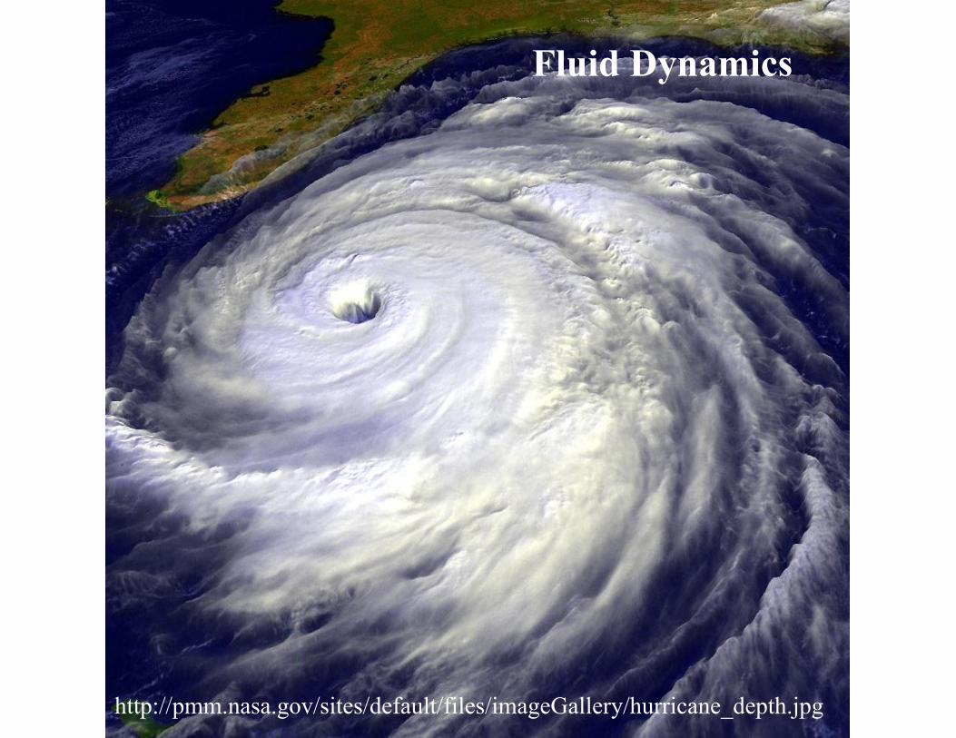
http://pmm.nasa.gov/sites/default/files/imageGallery/hurricane_depth.jpg
Fluid Dynamics

http://www.noaanews.noaa.gov/stories/images/hurricaneflying2.jpg
Dynamics of Turbulence

http://simulationresearch.lbl.gov/modelica/releases/msl/3.2/help/Modelica_Electrical_Analog_Examples.html
Chua Circuit
Electrical Dynamics

http://www.giss.nasa.gov/research/briefs/hansen_03/oceana_ts.gif
Climate dynamics
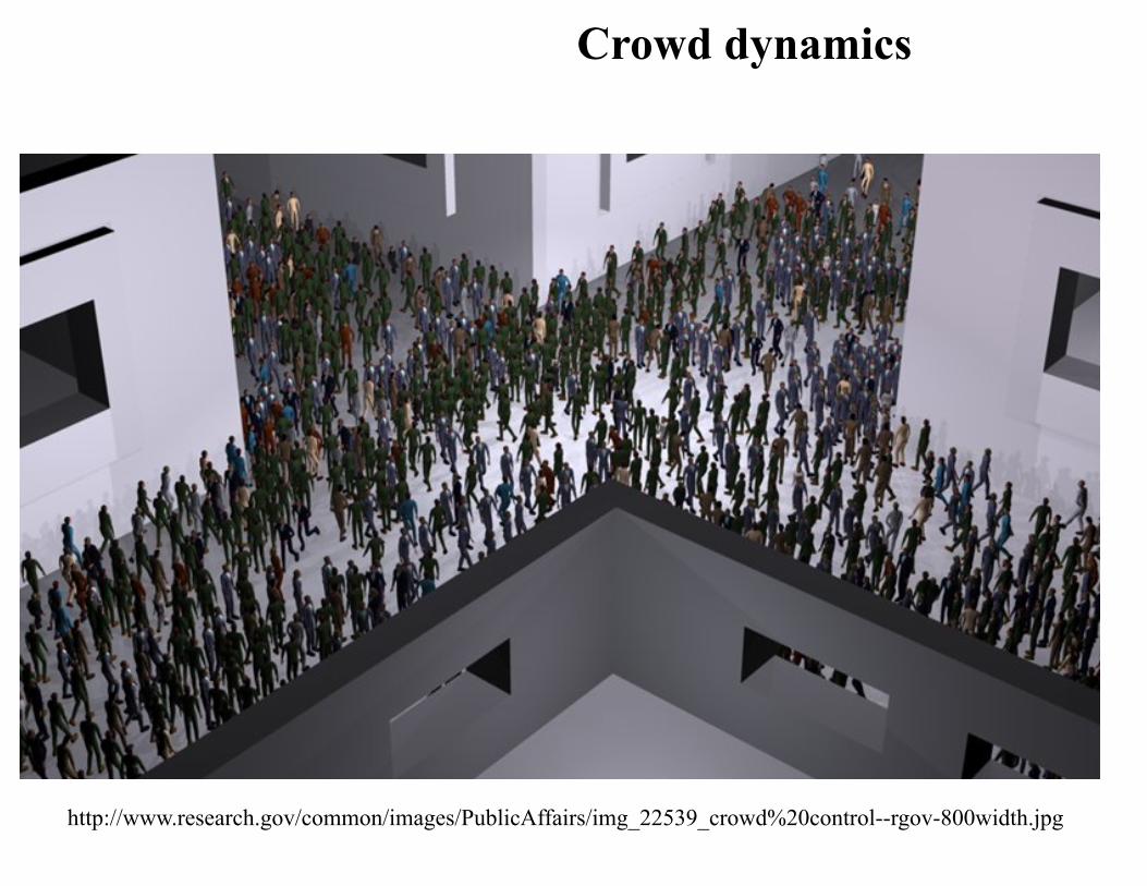
http://www.research.gov/common/images/PublicAffairs/img_22539_crowd%20control--rgov-800width.jpg
Crowd dynamics
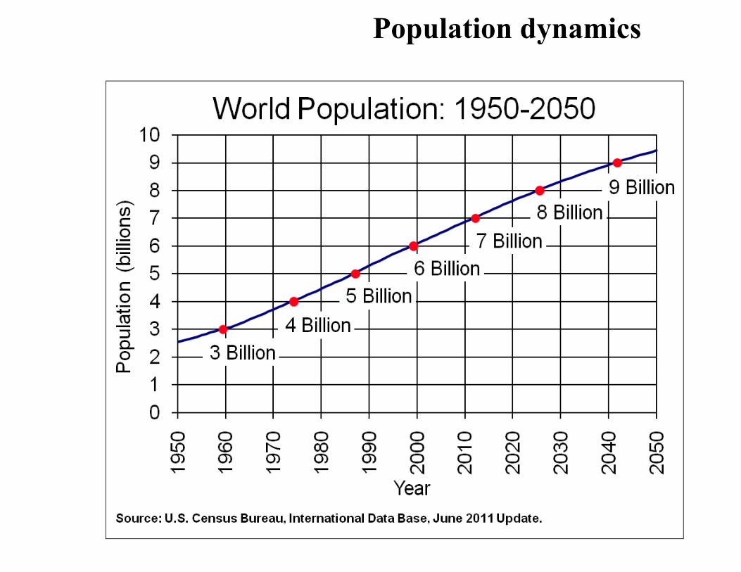
Population dynamics
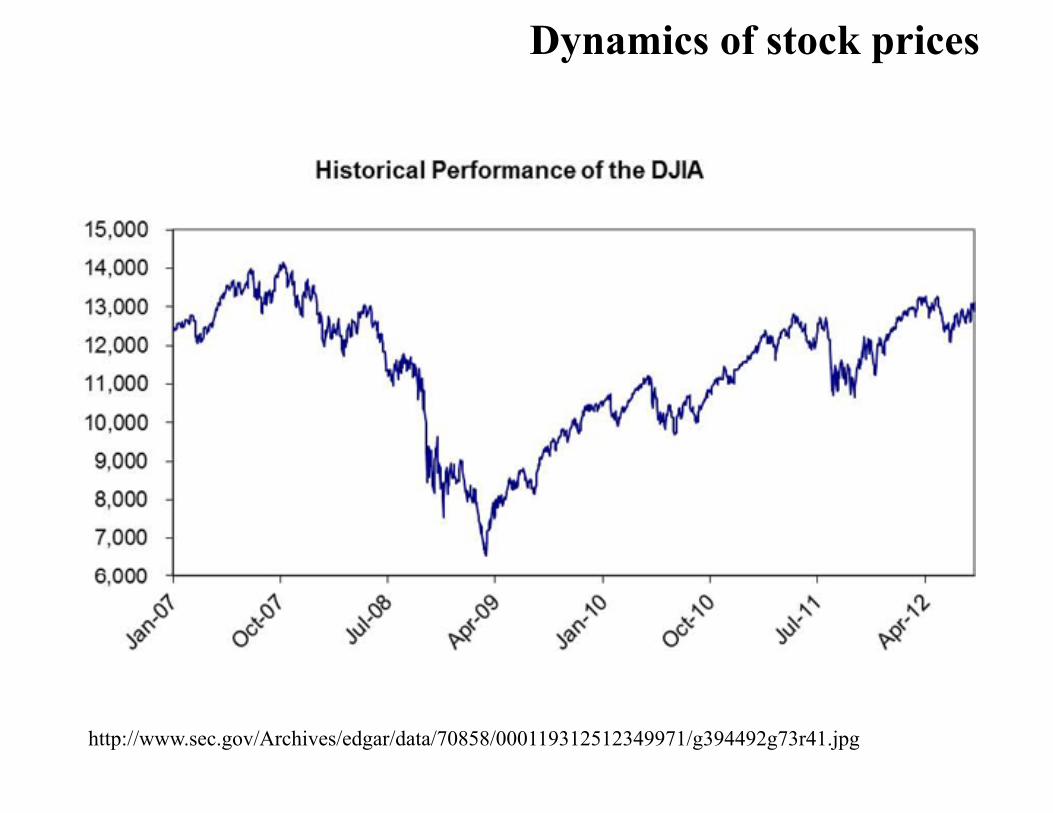
http://www.sec.gov/Archives/edgar/data/70858/000119312512349971/g394492g73r41.jpg
Dynamics of stock prices
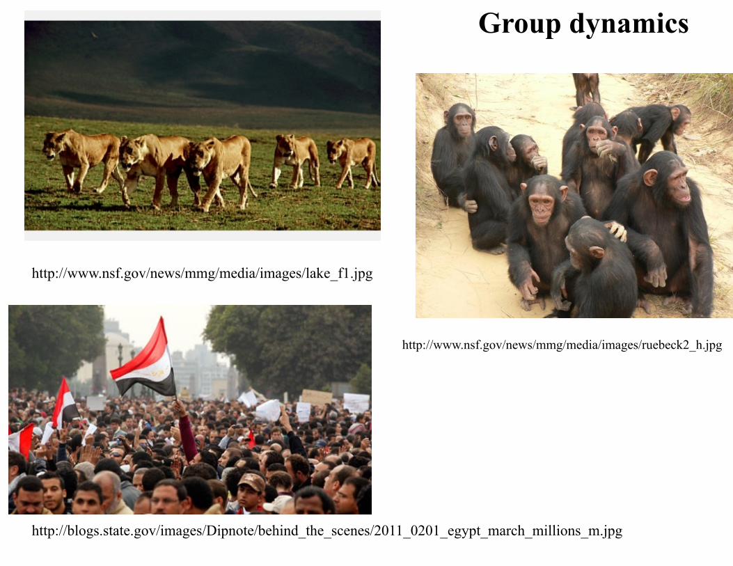
http://www.nsf.gov/news/mmg/media/images/ruebeck2_h.jpg
http://www.nsf.gov/news/mmg/media/images/lake_f1.jpg
http://blogs.state.gov/images/Dipnote/behind_the_scenes/2011_0201_egypt_march_millions_m.jpg
Group dynamics
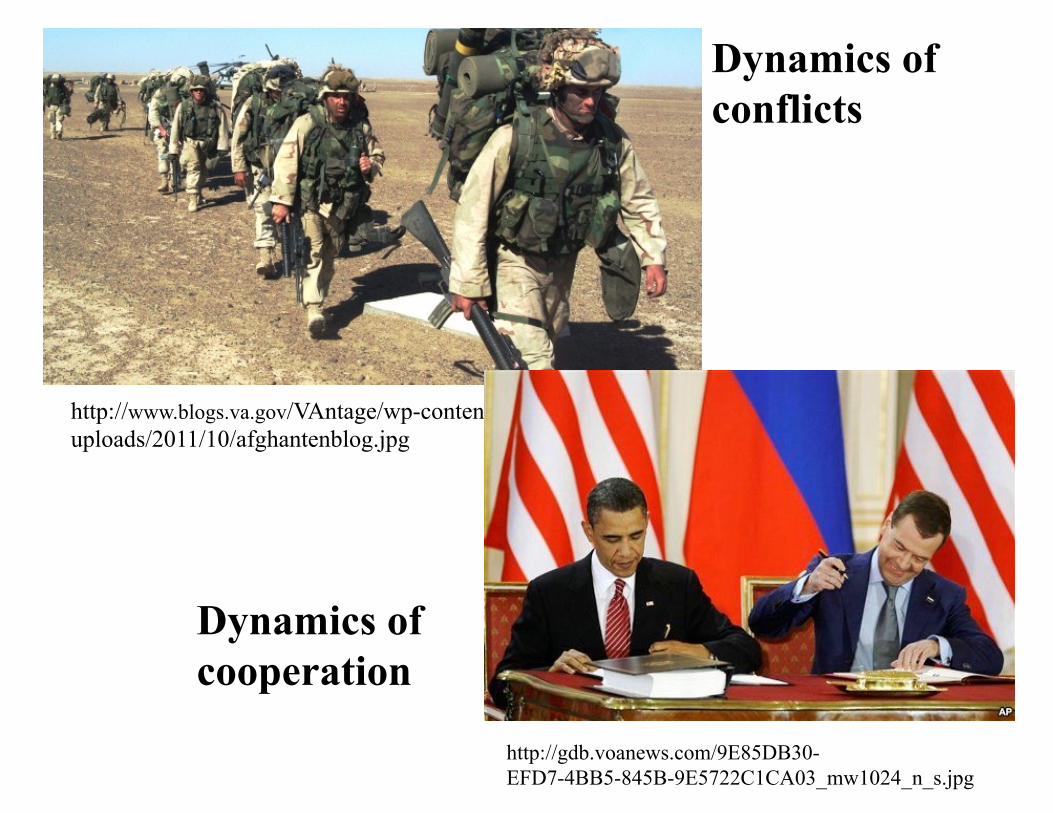
http://www.blogs.va.gov/VAntage/wp-content/uploads/2011/10/afghantenblog.jpg
http://gdb.voanews.com/9E85DB30-EFD7-4BB5-845B-9E5722C1CA03_mw1024_n_s.jpg
Dynamics of conflicts
Dynamics of cooperation

Dynamical Systems Theory:
– The branch of mathematics of how systems change over time • Calculus • Differential equations • Iterated maps • Algebraic topology • etc.
– The dynamics of a system: the manner in which
the system changes
– Dynamical systems theory gives us a vocabulary and set of tools for describing dynamics
Copyright © by Melanie Mitchell Conference on Complex Systems, September, 2015
A brief history of the science of dynamics
Copyright © by Melanie Mitchell Conference on Complex Systems, September, 2015

Aristotle, 384 – 322 BC

Nicolaus Copernicus, 1473 – 1543

Galileo Galilei, 1564 – 1642

Isaac Newton, 1643 – 1727
Pierre- Simon Laplace, 1749 – 1827
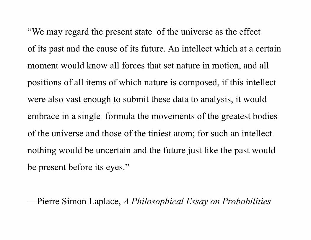
“We may regard the present state of the universe as the effect
of its past and the cause of its future. An intellect which at a certain
moment would know all forces that set nature in motion, and all
positions of all items of which nature is composed, if this intellect
were also vast enough to submit these data to analysis, it would
embrace in a single formula the movements of the greatest bodies
of the universe and those of the tiniest atom; for such an intellect
nothing would be uncertain and the future just like the past would
be present before its eyes.”
—Pierre Simon Laplace, A Philosophical Essay on Probabilities

Henri Poincaré, 1854 – 1912

“If we knew exactly the laws of nature and the situation of the
universe at the initial moment, we could predict exactly the
situation of that same universe at a succeeding moment. but
even if it were the case that the natural laws had no longer any
secret for us, we could still only know the initial situation
approximately. If that enabled us to predict the succeeding
situation with the same approximation, that is all we require,
and we should say that the phenomenon had been predicted,
that it is governed by laws. But it is not always so; it may
happen that small differences in the initial conditions
produce very great ones in the final phenomena. A small
error in the former will produce an enormous error in the latter.
Prediction becomes impossible...”
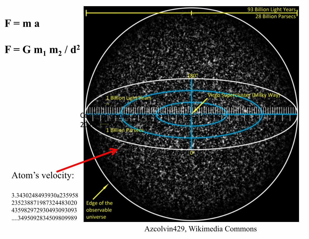
F = m a F = G m1 m2 / d2
Azcolvin429, Wikimedia Commons
Atom’s velocity: 3.3430248493930a235958 235238871987324483020 435982972930493093093 ....3495092834509809989
Conference on Complex Systems, September, 2015
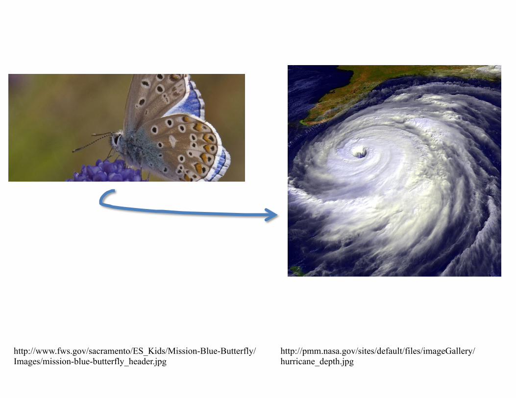
http://www.fws.gov/sacramento/ES_Kids/Mission-Blue-Butterfly/Images/mission-blue-butterfly_header.jpg
http://pmm.nasa.gov/sites/default/files/imageGallery/hurricane_depth.jpg
“You've never heard of Chaos theory? Non-linear equations? Strange attractors?”
Dr. Ian Malcolm
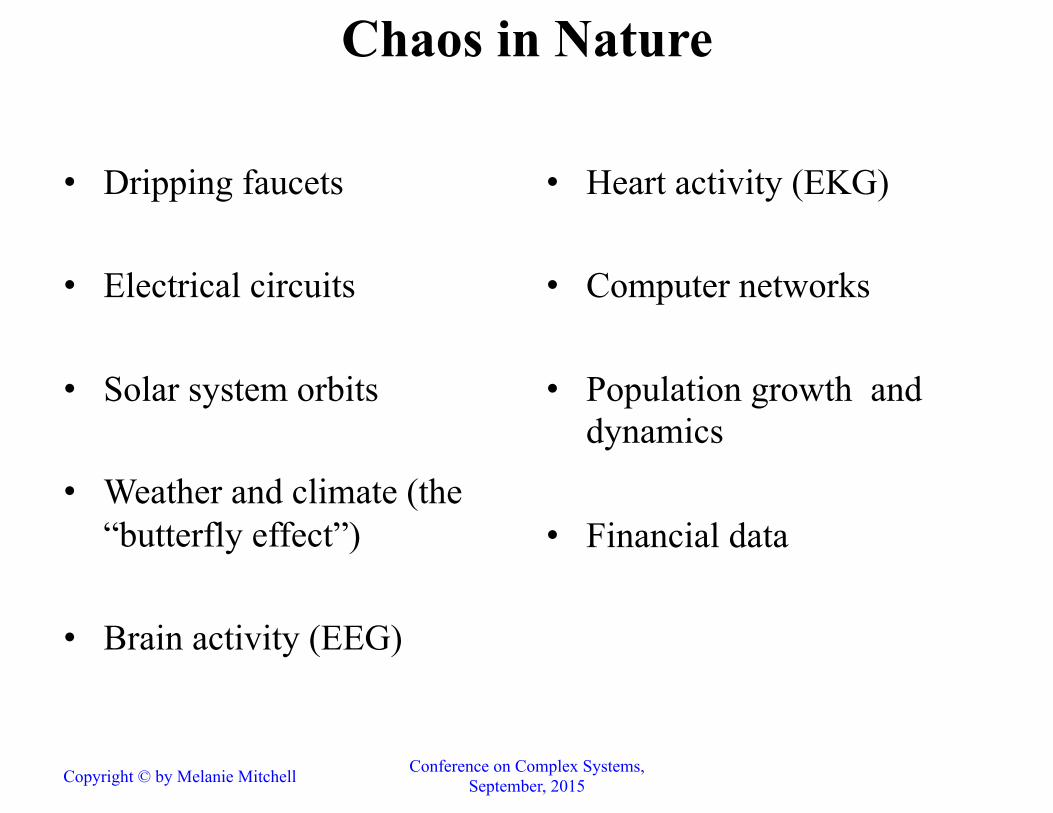
• Dripping faucets
• Electrical circuits
• Solar system orbits
• Weather and climate (the “butterfly effect”)
• Brain activity (EEG)
• Heart activity (EKG)
• Computer networks • Population growth and
dynamics
• Financial data
Chaos in Nature
Copyright © by Melanie Mitchell Conference on Complex Systems, September, 2015
What is the difference between chaos and randomness?
Notion of “deterministic chaos”
Copyright © by Melanie Mitchell Conference on Complex Systems, September, 2015

A simple example of deterministic chaos:
Exponential versus logistic models for population growth
€
nt+1 = 2nt
“Exponential” model: Each year each pair of parents mates, creates four offspring, and then parents die.
Copyright © by Melanie Mitchell Conference on Complex Systems, September, 2015

0
100000
200000
300000
400000
500000
600000
1 2 3 4 5 6 7 8 9 10 11 12 13 14 15 16 17 18 19
Popula@on n
Year
Exponential behavior: Population size vs. year
€
nt = 2t n0
Copyright © by Melanie Mitchell Conference on Complex Systems, September, 2015
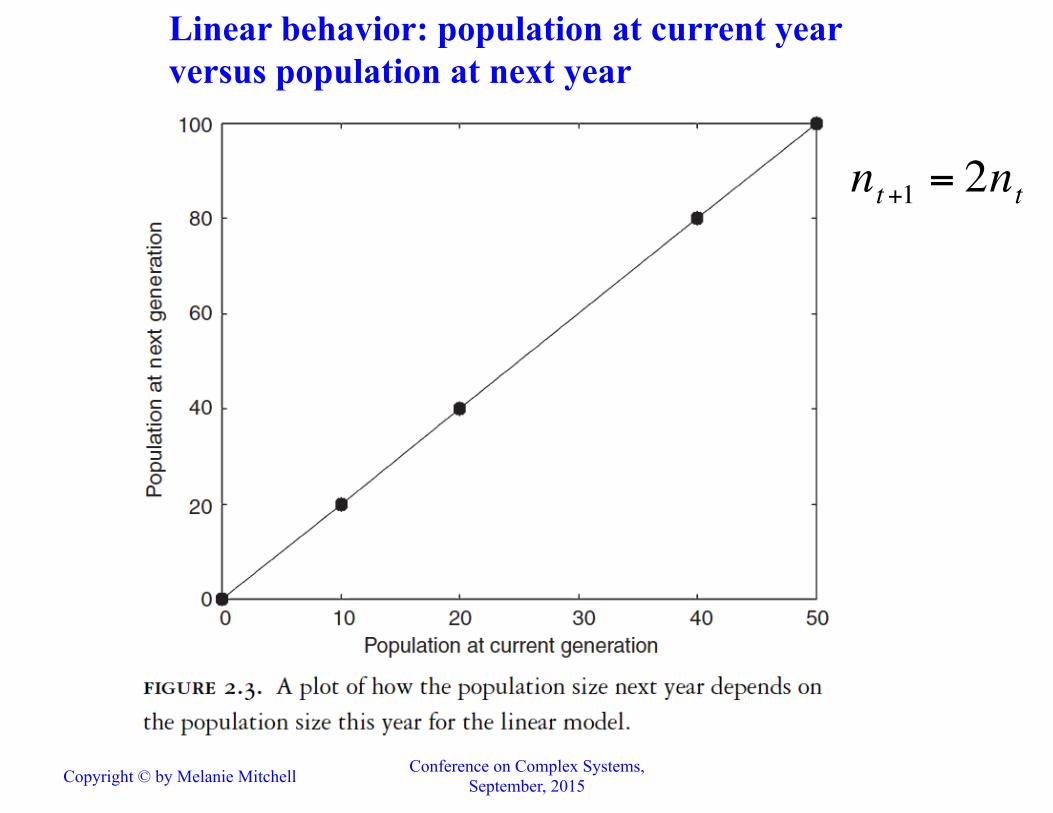
Linear behavior: population at current year versus population at next year
€
nt+1 = 2nt
Copyright © by Melanie Mitchell Conference on Complex Systems, September, 2015
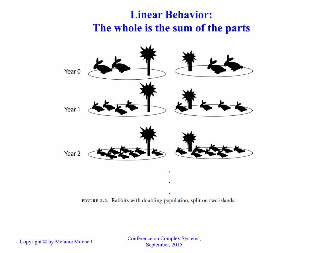
Linear Behavior: The whole is the sum of the parts
Copyright © by Melanie Mitchell Conference on Complex Systems, September, 2015
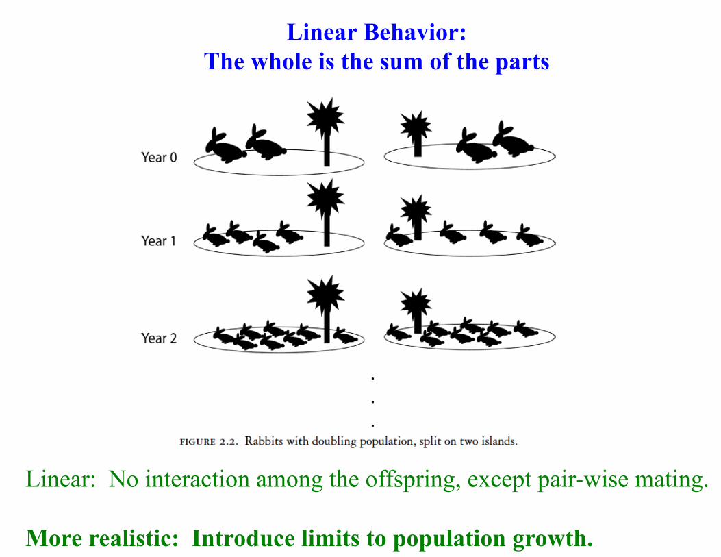
Linear: No interaction among the offspring, except pair-wise mating. More realistic: Introduce limits to population growth.
Linear Behavior: The whole is the sum of the parts
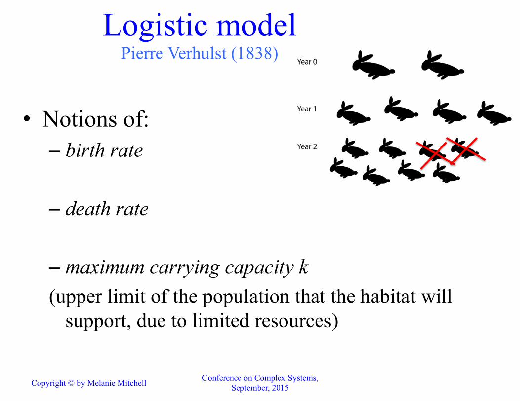
Logistic model Pierre Verhulst (1838)
• Notions of: – birth rate
– death rate
– maximum carrying capacity k (upper limit of the population that the habitat will
support, due to limited resources)
Copyright © by Melanie Mitchell Conference on Complex Systems,
September, 2015

Logistic model • Notions of: – birth rate and death rate – maximum carrying capacity k (upper limit of the population that the habitat
will support due to limited resources)
€
nt+1 = birthrate × nt − deathrate× nt= (b − d)nt
€
nt+1 = (b − d)ntk − ntk
#
$ %
&
' (
= (b − d) knt − nt2
k#
$ %
&
' (
interac(ons between offspring make this model nonlinear

€
nt+1 = (birthrate − deathrate)[knt − nt2]/k
Nonlinear Behavior
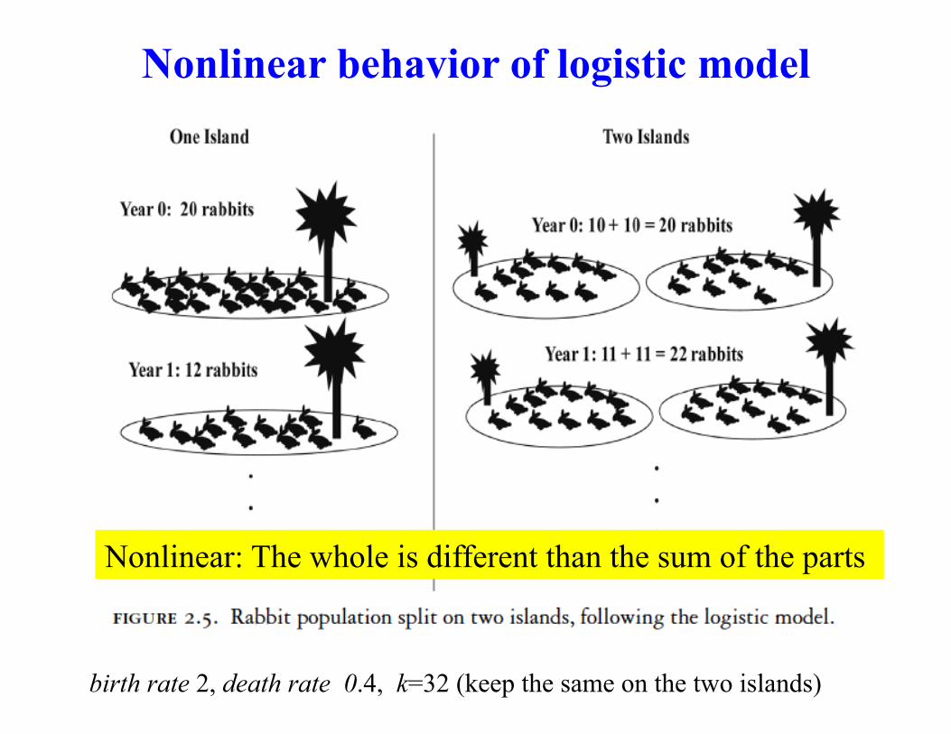
Nonlinear behavior of logistic model
birth rate 2, death rate 0.4, k=32 (keep the same on the two islands)
Nonlinear: The whole is different than the sum of the parts
aaa
€
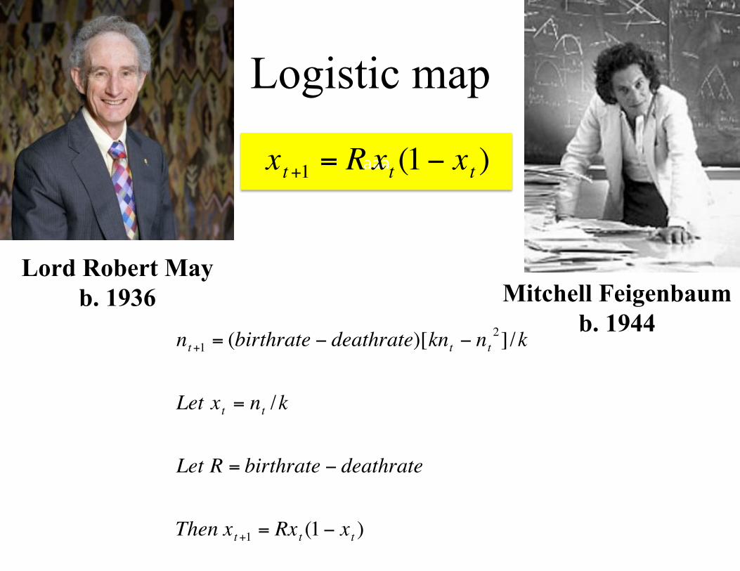
xt+1 = R xt (1− xt )
Logistic map
Lord Robert May b. 1936
€
nt+1 = (birthrate − deathrate)[knt − nt2]/k
Let xt = nt /k
Let R = birthrate − deathrate
Then xt+1 = Rxt (1− xt )
Mitchell Feigenbaum b. 1944
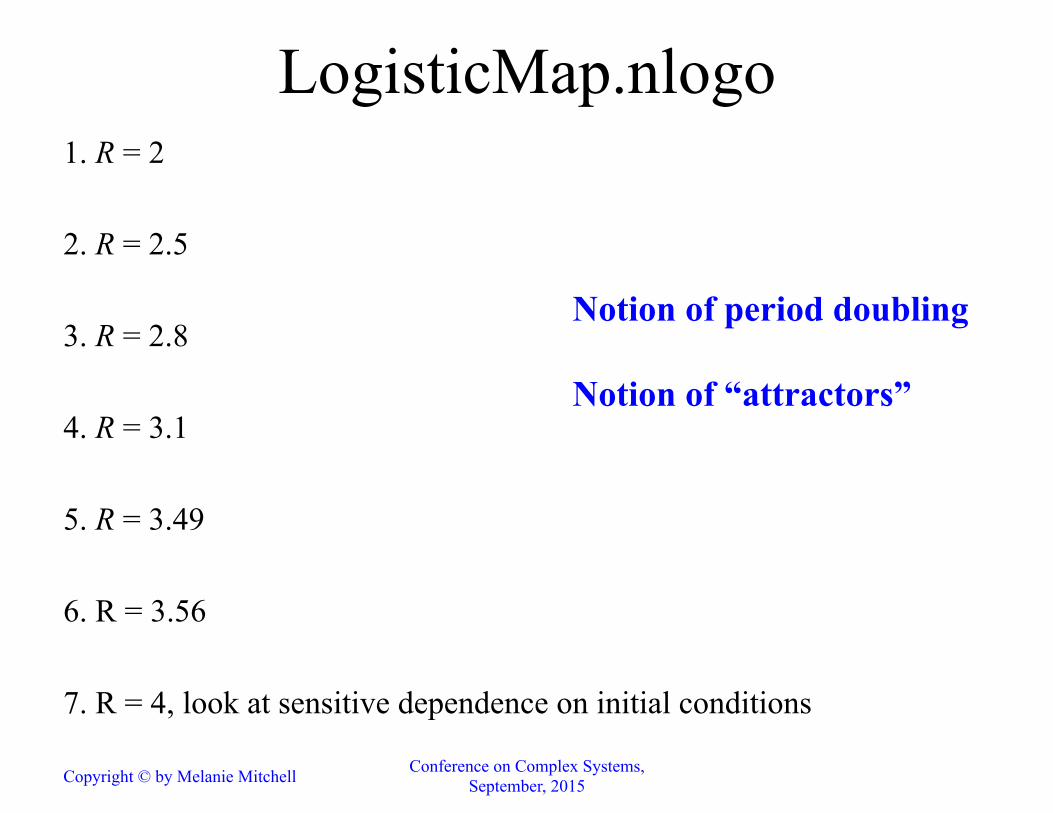
LogisticMap.nlogo 1. R = 2
2. R = 2.5 3. R = 2.8 4. R = 3.1 5. R = 3.49 6. R = 3.56 7. R = 4, look at sensitive dependence on initial conditions
Notion of period doubling Notion of “attractors”
Copyright © by Melanie Mitchell Conference on Complex Systems, September, 2015
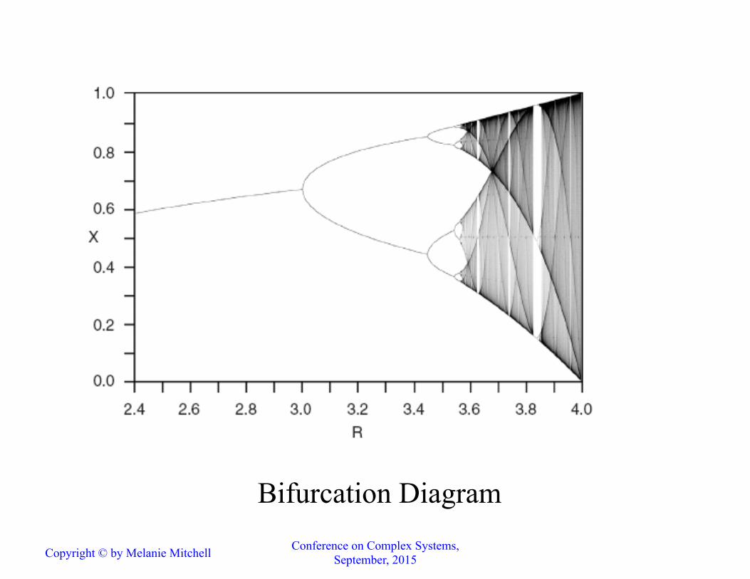
Bifurcation Diagram
Copyright © by Melanie Mitchell Conference on Complex Systems, September, 2015

“The fact that the simple and deterministic equation [i.e., the Logistic
Map] can possess dynamical trajectories which look like some sort of
random noise has disturbing practical implications. It means, for example,
that apparently erratic fluctuations in the census data for an animal
population need not necessarily betoken either the vagaries of an
unpredictable environment or sampling errors; they may simply derive
from a rigidly deterministic population growth relationship...Alternatively,
it may be observed that in the chaotic regime, arbitrarily close initial
conditions can lead to trajectories which, after a sufficiently long time,
diverge widely. This means that, even if we have a simple model in which
all the parameters are determined exactly, long-term prediction is
nevertheless impossible”
−− Robert May, 1976

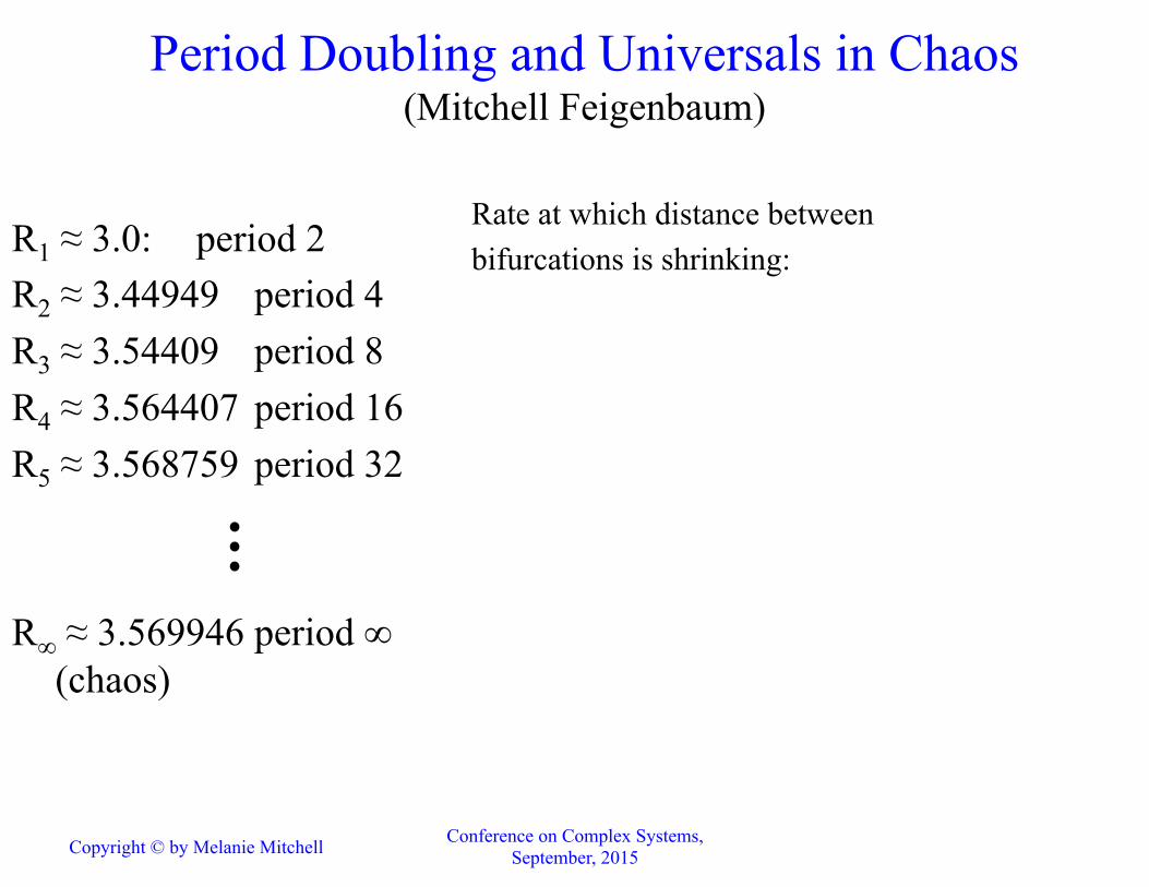
R1 ≈ 3.0: period 2 R2 ≈ 3.44949 period 4 R3 ≈ 3.54409 period 8 R4 ≈ 3.564407 period 16 R5 ≈ 3.568759 period 32 R∞ ≈ 3.569946 period ∞
(chaos)
A similar “period doubling route” to chaos is seen in any “one-humped (unimodal) map.
Period Doubling and Universals in Chaos (Mitchell Feigenbaum)
Copyright © by Melanie Mitchell Conference on Complex Systems, September, 2015
R1 ≈ 3.0: period 2 R2 ≈ 3.44949 period 4 R3 ≈ 3.54409 period 8 R4 ≈ 3.564407 period 16 R5 ≈ 3.568759 period 32 R∞ ≈ 3.569946 period ∞
(chaos)
Rate at which distance between bifurcations is shrinking:
Period Doubling and Universals in Chaos (Mitchell Feigenbaum)
Copyright © by Melanie Mitchell Conference on Complex Systems, September, 2015

R1 ≈ 3.0: period 2 R2 ≈ 3.44949 period 4 R3 ≈ 3.54409 period 8 R4 ≈ 3.564407 period 16 R5 ≈ 3.568759 period 32 R∞ ≈ 3.569946 period ∞
(chaos)
Rate at which distance between bifurcations is shrinking:
€
R2 − R1
R3 − R2
=3.44949 − 3.0
3.54409 − 3.44949= 4.75147992
R3 − R2
R4 − R3
=3.54409 − 3.44949
3.564407 − 3.54409= 4.65619924
R4 − R3
R5 − R4
=3.564407 − 3.54409
3.568759 − 3.564407= 4.66842831
limn→∞
Rn+1 − Rn
Rn+2 − Rn+1
%
& '
(
) * ≈ 4.6692016
Period Doubling and Universals in Chaos (Mitchell Feigenbaum)
Copyright © by Melanie Mitchell Conference on Complex Systems, September, 2015

€
R2 − R1
R3 − R2
=3.44949 − 3.0
3.54409 − 3.44949= 4.75147992
R3 − R2
R4 − R3
=3.54409 − 3.44949
3.564407 − 3.54409= 4.65619924
R4 − R3
R5 − R4
=3.564407 − 3.54409
3.568759 − 3.564407= 4.66842831
limn→∞
Rn+1 − Rn
Rn+2 − Rn+1
%
& '
(
) * ≈ 4.6692016
Period Doubling and Universals in Chaos (Mitchell Feigenbaum)
R1 ≈ 3.0: period 2 R2 ≈ 3.44949 period 4 R3 ≈ 3.54409 period 8 R4 ≈ 3.564407 period 16 R5 ≈ 3.568759 period 32 R∞ ≈ 3.569946 period ∞
(chaos)
Rate at which distance between bifurcations is shrinking:
In other words, each new bifurcation appears about 4.6692016 times faster than the previous one.
This same rate of 4.6692016 occurs in any unimodal map.
Copyright © by Melanie Mitchell Conference on Complex Systems, September, 2015

Amazingly, at almost exactly the same time, the same
constant was independently discovered (and
mathematically derived by) another research team, the
French mathematicians Pierre Collet and Charles Tresser.
Copyright © by Melanie Mitchell Conference on Complex Systems, September, 2015
Summary Significance of dynamics and chaos
for complex systems
• Complex, unpredictable behavior from simple, deterministic rules
• Dynamics gives us a vocabulary for describing complex
behavior
• There are fundamental limits to detailed prediction
• At the same time there is universality: “Order in Chaos”
Copyright © by Melanie Mitchell Conference on Complex Systems, September, 2015
Top Related